RESPONSE SURFACE METHODOLOGY

(R S M)

Par

Mariam MAHFOUZ

2

Remember that:

General Planning Part I

A - Introduction to the RSM method

B - Techniques of the RSM method

C - Terminology

D - A review of the method of least squares Part II

A - Procedure to determine optimum

conditions – Steps of the RSM method

B – Illustration of the method with an example

3

4

A - Procedure to determine optimum conditions steps of the method

This method permits to find the settings of the input variables which produce the most desirable response values.

The set of values of the input variables which result in the most desirable response values is called the set of optimum conditions.

5

Steps of the method

The strategy in developing an empirical model through a sequential program of experimentation is as follows:

1. The simplest polynomial model is fitted to a set of data collected at the points of a first-order design.

2. If the fitted first-order model is adequate, the information provided by the fitted model is used to locate areas in the experimental region, or outside the experimental region, but within the boundaries of the operability region, where more desirable values of the response are suspected to be.

6

3. In the new region, the cycle is repeated in that the first-order model is fitted and testing for adequacy of fit.

4. If nonlinearity in the surface shape is detected through the test for lack of fit of the first-order model, the model is upgraded by adding cross-product terms and / or pure quadratic terms to it. The first-order design is likewise augmented with points to support the fitting of the upgraded model.

7

5. If curvature of the surface is detected and a fitted second-order model is found to be appropriate, the second-order model is used to map or describe the shape of the surface, through a contour plot, in the experimental region.

6. If the optimal or most desirable response values are found to be within the boundaries of the experimental region, then locating the best values as well as the settings of the input variables that produce the best response values.

8

7. Finally, in the region where the most desirable response values are suspected to be found, additional experiments are performed to verify that this is so.

9

B- Illustration of the method with an

example

For simplicity of presentation we shall assume that there is only one response variable to be studied although in practice there can be several response variables that are under investigation simultaneously.

10

Experience

Chemical reaction

Two controlled Factors

Temperature (X1)

Time (X2)

One response

percent yield

An experimenter, interested in determining if an increase in the percent yield is possible by varying

the levels of the two factors.

11

Two levels of temperature: 70° and 90°.

Two levels of time: 30 sec and 90 sec.

Four temperature-time settings

(factorial combinations)

And two repetitions at each point

Four different design points

The total number of observations is N = 8

12

Detail

The response of interest is the percent yield, which is a measure of the purity of the end product.

The process currently operates in a range of percent purity between 55 % and 75 %, but it is felt that a higher percent yield is possible.

13

Design 1

Original variables Coded variables Percent yield

Temperature

X1 (C°)

Time

X2 (sec.)x1 x2 Y

70 30 -1 -149.8

48.1

90 30 1 -157.3

52.3

70 90 -1 165.7

69.4

90 90 1 173.1

77.8

x1 and x2 are the coded variables which are defined as:

10

8011

X

x 30

6022

X

x

14

Representation of the first design

15

First-order model

Expressed in terms of the coded variables, the observed percent yield values are modeled as:

The remaining term, , represents random error in the yield values.

The eight observed percent yield values, when expressed as function of the levels of the coded variables, in matrix notation, are:

Y = X +

22110 xxY

16

Matrix form

= +

8.77

1.73

4.69

7.65

3.52

3.57

1.48

8.49

111

111

111

111

111

111

111

111

2

1

0

8

7

6

5

4

3

2

1

Vector of response values

Matrix of the design

Vector of unknown parameters

Vector of error terms

17

Estimations

The estimates of the coefficients in the first-order model are found by solving the normal equations:

The estimates are:

The fitted first-order model in the coded variables is:

YXXbX

8125.9

4375.3

6875.611 YXXXb

21 8125.94375.36875.61)(ˆ xxxY

18

ANOVA table – design 1

SourceDegrees of freedom

d.f.

Sum of squares

SS

Mean square

F

Model 2 864.8125 432.4063 63.71

Residual 5 33.9363 6.7873

Lack of fit 1 2.1013 2.1013 0.264

Pure error 4 31.8350 7.9588

Test of adequacy

0: 210 H

19

Individual tests of parameters

To do that the Student-test is used.

For the test of: we have

And for we have

Each of the null hypotheses is rejected at the = 0.05 level of significance owing to the calculated values, 3.73 and 10.65, being greater in absolute value than the tabled value,

T5;0.025 =2.571.

0: 10 H 73.3)var(

0

1

1

b

bt

0: 20 H 65.10)var(

0

2

2

b

bt

20

Conclusion of the first analysis

The first – order model is adequate.

That both temperature and time have an effect on percent yield.

Since both b1 and b2 are positive, the effects are positive.

Thus, by raising either the temperature or time of reaction, this produced a significant increase in percent yield.

21

Second stage of the sequential program

At this point, the experimenter quite naturally might ask:

If additional experiments can be performed

At what settings of temperature and time should the additional experiments be run?”

To answer this question, we enter the second stage of our sequential program of

experimentation.

22

Contour plots

The fitted model:

can now be used to map values of the estimated response surface over the experimental region.

This response surface is a hyper-plane; their contour plots are lines in the experimental region.

The contour lines are drawn by connecting two points (coordinate settings of x1 and x2) in the experimental region that produce the same value of

21 8125.94375.36875.61)(ˆ xxxY

Y

23

In the figure above are shown the contour lines of the estimated planar surface for percent yield corresponding to values of = 55, 60, 65 and 70 %.)(ˆ xY

24

Performing experiments along the path of steepest ascent

To describe the method of steepest ascent mathematically, we begin by assuming the true response surface can be approximated locally with an equation of a hyper-plane

Data are collected from the points of a first-order design and the data are used to calculate the coefficient estimates to obtain the fitted first-order model

k

iii x

10

k

iii xbbxY

10)(ˆ

Estimated response function

25

The next step is to move away from the center of the design, a distance of r units, say, in the direction of the maximum increase in the response.

By choosing the center of the design in the coded variable to be denoted by O(0, 0, …, 0), then movement away from the center r units is equivalent to find the values of which maximize

subject to the constraint Maximization of the response function is

performed by using Lagrange multipliers. Let

where is the Lagrange multiplier.

kxxx ,...,, 21

k

iiixbbxY

10)(ˆ

2

1

2 rxk

ii

2

1

2

1021 ),...,,( rxxbbxxxQ

k

ii

k

iiik

26

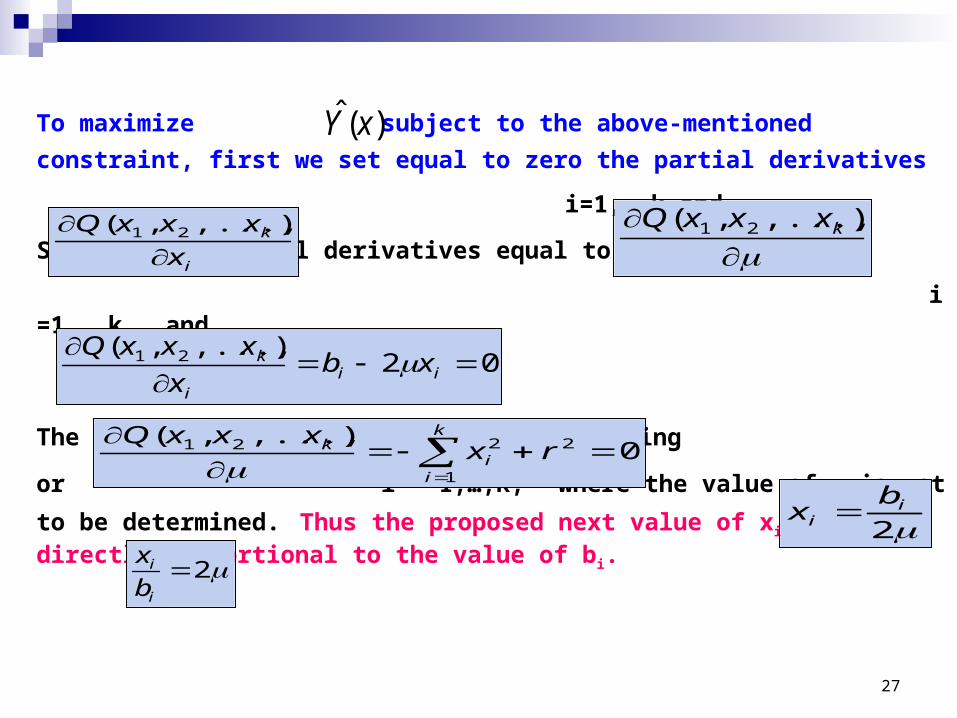
27

To maximize subject to the above-mentioned constraint,

first we set equal to zero the partial derivatives i=1,…,k and

Setting the partial derivatives equal to zero produces: i =1,…,k, and

The solutions are the values of xi satisfying

or i = 1,…,k, where the value of is yet to be determined. Thus the proposed next value of xi is directly proportional to the value of bi.

)(ˆ xY

i

k

x

xxxQ

),...,,( 21

),...,,( 21 kxxxQ

02),...,,( 21

iii

k xbx

xxxQ

0),...,,( 2

1

221

rxxxxQ k

ii

k

2i

i

bx

2i

i

b

x

28

Let us the change in Xi be noted by i , and the change in xi be noted by i. The coded variables is obtained by these formulas where

(respectively si) is the mean (respectively the standard deviation) of the two levels of Xi .

Thus , then

or

i

iii s

XXx

iX

i

iiiii s

XXx

)(

i

ii s

iii s

29

Let us illustrate the procedure with the fitted first-order model:

that was fitted early to the percent yield values in our example.

To the change in X2, 2=45 sec. corresponds the change in x2, 2=45/30=1.5 units.

In the relation , we can substitute i to xi:

, thus and 1 = 0.526, so

1=0.526*10=5.3°C .

21 8125.94375.36875.61)(ˆ xxxY

2

2

1

1

b

x

b

x

2

2

1

1

bb

8125.9

5.1

4375.31

30

Points along the path of steepest ascent and observed percent yield values at the points

Temperature

X1 (°C)

Time

X2 (sec.)Observed

percent yield

Base 80.0 60

i 5.3 45

Base + i 85.3 105 74.3

Base + 1.5 i 87.95 127.5 78.6

Base + 2 I 90.6 150 83.2

Base + 3 I 95.9 195 84.7

Base + 4 i 101.2 240 80.1

31

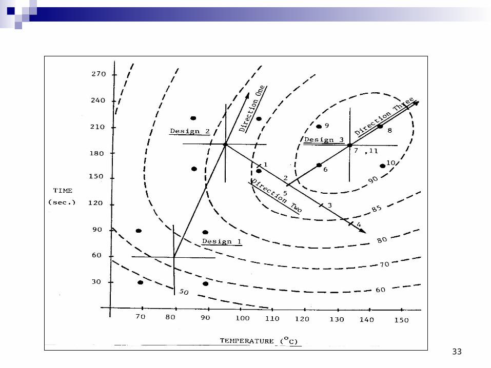
32

Sequence of experimental trials performed in moving to a region of high percent yield values

Design two: For this design the coded variables are defined as:

x1 x2 X1 X2 % yield

-1 -1 85.9 165 82.9; 81.4

+1 -1 105.9 165 87.4; 89.5

-1 +1 85.9 225 74.6; 77.0

+1 +1 105.9 225 84.5; 83.1

0 0 95.9 195 84.7; 81.9

10

9.95)( 11

XeTemperaturx 30

195)( 22

XTimex

33

34

The fitted model corresponding to the group of experiments

of design two is:

The corresponding analysis of variance is: 21 750.2575.370.82)(ˆ xxxY

Source d.f. SS MS F

Model 2 162.745 81.372 42.34

Residual 7 13.455 1.922

Lack of fit 2 2.345 1.173 0.53

Pure error 5 11.110 2.222

Total (variations)

9 176.2

The model is jugged adequate

35

sequence of experimental trials that were performed in the direction two:

Steps x1 x2 X1 X2 % yield

1 Center + i +1 - 0.77 105.9 171.9 89.0

2 Center + 2 i +2 - 1.54 115.9 148.8 90.2

3 Center + 3 i +3 - 2.31 125.9 125.7 87.4

4 Center + 4 i +4 - 3.08 135.9 102.6 82.6

36

37

Retreat to center + 2 i and proceed in direction three

Steps x1 x2 X1 X2 % yield

5

Replicated 2+2 - 1.54 115.9 148.8 91.0

6 +3 - 0.77 125.9 171.9 93.6

7 +4 0 135.9 195 96.2

8 +5 0.77 145.9 218.1 92.9

38

Set up design three using points of steps 6, 7,

and 8 along with the following two points:

Steps x1 x2 X1 X2 % yield

9 +3 0.77 125.9 218.1 91.7

10 +5 - 0.77 145.9 171.9 92.5

11

Replicated 7+4 0 135.9 195 97.0

39

40

Design three was set up using the point at step 7 as its center. It includes steps 6 – 11. If we redefine the coded

variables: and

then the fitted first-order model is:

The corresponding analysis of variance table is:

10

9.135)( 11

XeTemperaturx 1.23

195)( 21

XTimex

21 375.0025.0983.93)(ˆ xxxY

41

ANOVA table

source d.f. SS MS F

Model 2 0.5650 0.2825 0.04

Residual 3 22.1833 7.3944

total 5 22.7483

It is obvious from the ANOVA table that the least model does not explain a significant amount of the overall variation in the percent yield values, and it is necessary to fit a curved surface.

42

Fitting a second-order model

A second-order model in k variables is of the form:

The number of terms in the model above is p=(k+1)(k+2)/2; for example, when k=2 then p=6.

Let us return to the chemical reaction example of the previous section. To fit a second-order model (k=2), we must perform some additional experiments.

ji

jiij

k

iiii

k

iii xxxxY

1

2

10

43

Central composite rotatable design

Suppose that four additional experiments are performed, one at each of the axial settings (x1,x2):

These four design settings along with the four factorial settings: (-1,-1); (-1,1); (1,-1); (1,1) and center point comprise a central composite rotatable design.

The percent yield values and the corresponding nine design settings are listed in the table below:

)2,0();2,0();0,2();0,2(

44

Central composite rotatable design

45

Percent yield values at the nine points of a central composite rotatable design

46

The fitted second-order model, in the coded variables, is:

The analysis is detailed in this table, using the RSREG procedure in the SAS software:

2122

2121 58.083.198.131.003.06.96)(ˆ xxxxxxxY

47

SAS output 1 2122

2121 58.083.198.131.003.06.96)(ˆ xxxxxxxY

48

SAS output 2

49

Response surface and the contour plot

50

More explanations

The contours of the response surface, showing above, represent predicted yield values of 95.0 to 96.5 percent in steps of 0.5 percent.

The contours are elliptical and centered at the point

(x1; x2)=(- 0.0048; - 0.0857)

or (X1; X2)=(135.85°C; 193.02 sec). The coordinates of the centroid point are called the

coordinates of the stationary point. From the contour plot we see that as one moves

away from the stationary point, by increasing or decreasing the values of either temperature or time, the predicted percent yield (response) value decreases.

51

52

Determining the coordinates of the stationary point

A near stationary region is defined as a region where the surface slopes (or gradients along the variables axes) are small compared to the estimate of experimental error.

The stationary point of a near stationary region is the point at which the slope of the response surface is zero when taken in all direction.

The coordinates of the stationary point are calculated by differentiating the estimated response equation with respect to each xi, equating these derivatives to zero, and solving the resulting k equations simultaneously.

),...,,( 020100 kxxxx

53

Remember that the fitted second-order model in k variables is:

To obtain the coordinates of the stationary point, let us write the above model using matrix notation, as:

ji

jiij

k

iiii

k

iii xxbxbxbbxY

1

2

10)(ˆ

BxxbxbxY 0)(ˆ

54

where

and

kx

x

x

x

.

.

.2

1

kb

b

b

b

.

.

.2

1

kk

k

k

b

symetric

bb

bbb

B

..

..

..2

...

2...

22

22

11211

BxxbxbxY 0)(ˆ

55

Some details

The partial derivatives of with respect to x1, x2, …, xk are :

)(ˆ xY

Bxb

xbbbx

xY

xbbbx

xY

xbxbbx

xY

k

jjkjkkk

k

k

jjj

k

jjj

2

2)(ˆ

.

.

.

2)(ˆ

2)(ˆ

1

1

22222

2

211111

1

56

More details

Setting each of the k derivatives equal to zero and solving for the values of the xi, we find that the coordinate of the stationary point are the values of the elements of the kx1 vector x0 given by:

At the stationary point, the predicted response value, denoted by , is obtained by substituting x0 for x:

2

1

0

bBx

0Y

2ˆ

'0

00'0

'000

bxbBxxbxbY

57

Return to our example

The fitted second-order model was:

so the stationary point is:

In the original variables, temperature and time of the chemical reaction example, the setting at the stationary point are: temperature=135.85°C and time=193.02 sec.

And the predicted percent yield at the stationary point is:

2122

2121 58.083.198.131.003.06.96)(ˆ xxxxxxxY

83127.128750.0

28750.098127.1B

5588.008109.0

08109.051650.01B

08568.0

00486.0

2

1 10 bBx

613.96013.060.960 Y

58

Moore details

Note that the elements of the vector x0 do not tell us anything about the nature of the surface at the stationary point.

This nature can be a minimum, a maximum or a mini_max point.

For each of these cases, we are assuming that the stationary point is located inside the experimental region.

When, on the other hand, the coordinates of the stationary point are outside the experimental region, then we might have encountered a rising ridge system or a falling ridge system, or possibly a stationary ridge.

59

60

Nest Step

The next step is to turn our attention to expressing the response system in canonical form so as to be able to describe in greater detail the nature of the response system in the neighborhood of the stationary point.

61

The canonical Equation of a Second-Order Response System

The first step in developing the canonical equation for a k-variable system is to translate the origine of the system from the center of the design to the stationary point, that is, to move from (x1,x2,…,xk)=(0,0,…,0) to x0.

This is done by defining the intermediate variables (z1,z2,…,zk)=(x1-x10,x2-x20,…,xk-xk0) or z=x-x0.

Then the second-order response equation is expressed in terms of the values of zi as:

BzzY

xzBxzbxzbzY

0

0000

ˆ

)()()()(ˆ

62

Now, to obtain the canonical form of the predicted response equation, let us define a set of variables w1,w2,…,wk such that W’=(w1,w2,…,wk) is given by

where M is a kxk orthogonal matrix whose columns are eigenvectors of the matrix B.

The matrix M has the effect of diagonalyzing B, that is, where 1,2,…,k are the corresponding eigenvalues of B.

The axes associated with the variables w1,w2,…,wk are called the principal axes of the response system.

This transformation is a rotation of the zi axes to form the wi axes.

zMW

),...,,( 21 kdiagBMM

63

64

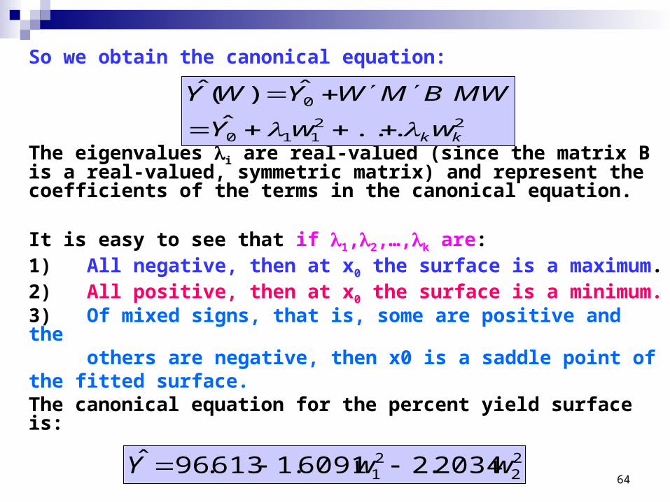
So we obtain the canonical equation:

The eigenvalues i are real-valued (since the matrix B is a real-valued, symmetric matrix) and represent the coefficients of the terms in the canonical equation.

It is easy to see that if 1,2,…,k are:1) All negative, then at x0 the surface is a maximum.2) All positive, then at x0 the surface is a minimum.3) Of mixed signs, that is, some are positive and the others are negative, then x0 is a saddle point of

the fitted surface.The canonical equation for the percent yield surface is:

22110

0

...ˆ

ˆ)(ˆ

kkwwY

MWBMWYWY

22

21 2034.26091.1613.96ˆ wwY

65

Moore details

The magnitude of the individual values of the i tell how quickly the surface height changes along the Wi axes as one moves away from x0.

Today there are computer software packages available that perform the steps of locating the coordinates of the stationary point, predict the response at the stationary point, and compute the eigenvalues and the eigenvectors.

66

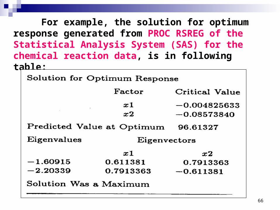
For example, the solution for optimum response generated from PROC RSREG of the Statistical Analysis System (SAS) for the chemical reaction data, is in following table:

67

RecapitulateProcess to

optimize

Input and outputvariables

Experimental andOperational regions

Series of experiments

Fitting First-order

model

ModelAdequate ?

Yes

Contours and optimal direction

No

Experiments in the Optimal direction

Locate a new Experimental region

New series of experiments

Fitting First-order

modelModel

Adequate ?

Yes

Fitting a Second-order

modelNo

68

Coordinates of the stationary point.

Description of the shape of the response surface

near the stationary point by contour plots.

Canonical analysis.

If needed, Ridge analysis (not detailed here).

Doing this:

69

Field of use of the method

In agriculture In food industry In pharmaceutical industry In all kinds of the light and heavy

industries In medical domain

Etc….

70

Bibliography André KHURI and John CORNELL: “Response

Surfaces – Designs and Analyses” , Dekker, Inc., ASQC Quality Press, New York.

Irwin GUTTMAN: “Linear Models: An Introduction”, John Wiley & Sons, New York.

George BOX, William HUNTER & J. Stuart HUNTER: “Statistics for experimenters: An Introduction to Design, Data Analysis, and Model Building” , John Wiley & Sons, New York.

George BOX & Norman DRAPPER: “Empirical Model-Building and Response Surfaces” , John Wiley & Sons, New York.

71