Response of velocity and turbulence in submerged wall jets to abrupt changes from smooth to rough beds and its application to scour downstream of an apron

J. Fluid Mech. (2006), vol. 556, pp. 387–419. c© 2006 Cambridge University Press

doi:10.1017/S0022112006009530 Printed in the United Kingdom

387

Response of velocity and turbulence insubmerged wall jets to abrupt changes fromsmooth to rough beds and its application to

scour downstream of an apron

By SUBHASISH DEY AND ARINDAM SARKARDepartment of Civil Engineering, Indian Institute of Technology, Kharagpur 721302,

West Bengal, India

(Received 15 August 2005 and in revised form 8 November 2005)

This paper addresses how the turbulent flow field in submerged wall jets responds toan abrupt change from smooth to rough beds. Experiments were conducted forsubmerged wall jets having different submergence factors and jet Froude numbers.The bed configurations investigated consisted of different combinations of the lengthsof smooth beds and the roughness of rough beds. The vertical profiles of time-averaged velocity components, turbulence intensity components and Reynolds stresswere detected by an acoustic Doppler velocimeter at different streamwise distances;and the horizontal distributions of bed shear stress were estimated from the Reynoldsstress profiles. The flow field displays the decay of jet velocity due to abrupt changesfrom smooth to rough beds. The boundary layer grows more quickly with increasein roughness of rough beds. The change in bed roughness induces an increaseddepression of the free surface over the smooth bed. The Reynolds and bed shearstresses are also computed by solving the Navier–Stokes equations. The responseof the turbulent flow characteristics of submerged wall jets to abrupt changes fromsmooth to rough beds is analysed from the point of view of similarity, growth ofthe length scale, and decay of the velocity and turbulence characteristics scales. Thesignificant observation is that the flow in the fully developed zone is plausibly self-preserving on both smooth and rough beds. Also, the use of a common length scalemakes it possible to collapse all the flow data onto a single band; and there is agradual variation of flow at the junction of the smooth and rough beds.

The equilibrium scour profiles downstream of a smooth apron due to submergedwall jets are computed from the threshold condition of the sediment particles on thescoured bed. Use of the modified bed shear stress for the downstream variation ofscoured bed permits the computation of the equilibrium scour profiles. The time-variation of maximum scour depth is computed from the bed shear stress with amodification for the time dependence. The agreement between the results obtainedfrom the model and the experimental data is satisfactory.

1. IntroductionWhen a submerged wall jet passes over a bed with an abrupt change in bed

roughness, the characteristics of velocity and turbulence are different from those ofthe corresponding jet over a homogenous rough bed as a result of the roughnessdiscontinuity. Most of the prior investigations on an abrupt change in bed roughnesswere on uniform flow in closed conduits or open channels (Townsend 1966; Antonia &

388 S. Dey and A. Sarkar

Luxton 1971; Schofield 1981; Nezu & Tominaga 1994; Chen & Chiew 2003). However,little attention has so far been paid to the flow characteristics of submerged wall jetson abrupt changes of bed roughness. The problem is not only important fromthe fundamental view point, but also in the context of its potential application todetermine the scour downstream of an apron due to submerged wall jets. To bemore explicit, when a submerged wall jet flows on a horizontal bed having an abruptchange in bed roughness, e.g. a smooth rigid bed (say an apron) followed by a roughsediment bed, it leads to a local scour downstream of the rigid apron.

Therefore, first the present study (experimental and theoretical) addresses how theflow and turbulence characteristics of horizontal submerged wall jets respond to anabrupt change from smooth to rough beds (§§ 3, 4, 5 and 6). Secondly, based onthese findings, it focuses on a methodology to determine the scour profiles and thetime-variation of scour of sediment beds downstream of an apron due to submergedjets issuing from a sluice opening (§ 7). Experiments were carried out on the scourdownstream of an apron to validate the analytical scour model.

When summarizing the previous studies along the lines of the present study, it isimportant to mention that Long, Steffler & Rajaratnam (1990) and Wu & Rajaratnam(1995) viewed the submerged wall jets as transitional phenomena between wall jetsand free jumps. Therefore, a brief outline of the important studies on wall jets, freejumps and submerged wall jets are given in addition to those on scour downstreamof an apron due submerged wall jets.

1.1. Studies on wall jets, free jumps and submerged wall jets

Based on the boundary layer theory, Glauert (1956) analysed the wall jet on ahorizontal bed. Schwarz & Cosart (1961) estimated the bed shear and Reynoldsstresses in a turbulent wall jet by solving the equations of motion for a steady turbulentflow. Rajaratnam (1967) measured the velocity and bed shear stress for plane turbulentwall jets on artificial rough beds, using Pitot and Preston tubes, respectively. Ead &Rajaratnam (2002) found that for low tailwater depths, the momentum flux of the flowin the wall jets decays appreciably with the distance due to the entrainment of reversedflow. Tachie, Balachandar & Bergstrom (2004) measured the flow characteristics of aplane turbulent wall jet and reported that the bed roughness is the cause of an increasethe inner-layer thickness, but the jet half-width is nearly independent of bed roughness.

Rajaratnam (1965) analysed the free (hydraulic) jump as a two-dimensional walljet. The mean velocity profiles in the outer layer of a free jump were found to be self-preserving when the velocity and length scales were used as issuing jet velocity and jetthickness, respectively. Rajaratnam (1968) observed the free jumps on rough beds to beconsiderably shorter than those on smooth bed. Hughes & Flack (1984) investigatedthe physical characteristics of the free jump on rough beds. They reported that the bedroughness is the cause of reduction of the tailwater depth and the length of the jump.Long et al. (1990) measured the velocity, turbulence intensity and Reynolds stresswith a laser Doppler anemometer to study the flow characteristics of submerged walljets on smooth bed. They found some degree of self-preserving flow characteristicsin the fully developed zone. Wu & Rajaratnam (1995) made a comparative studyamongst free jumps, submerged jumps and wall jets with the conclusion that thesubmerged wall jet is the transition between the wall jet and the free jump.

1.2. Studies on scour downstream of an apron due to submerged wall jets

Local scour downstream of an apron due to submerged wall jets was studied byChatterjee & Ghosh (1980), Hassan & Narayanan (1985), Dey & Westrich (2003)

Response of submerged wall jets to changes from smooth to rough beds 389

and Hopfinger et al. (2004). Chatterjee & Ghosh (1980) measured the velocity profilesin submerged wall jets as they develop over the apron followed by the scour hole.Hassan & Narayanan (1985) studied the flow characteristics and the similarity ofscour profiles downstream of an apron due to a submerged wall jet. They proposeda semi-empirical theory based on the characteristic mean velocity in the scour holeto predict the time-variation of scour depth. Dey & Westrich (2003) measured thevariation of the boundary layer thickness from the measured velocity profiles atdifferent streamwise locations (over the apron and within the scoured bed of cohesivesediments). They developed empirical relationships for the variation of the boundarylayer thickness and obtained an expression for bed shear stress from the solutionof the von Karman momentum integral equation. Recently, Hopfinger et al. (2004)described the scour process downstream of a short apron due to submerged jets andproposed a method to predict the time-variation of scour depth using the findingsof Hogg, Huppert & Dade (1997), who put forward a model to compute the scourprofiles due to horizontal turbulent wall jets without an apron.

2. Experimental setup and measurement techniquesExperiments were carried out in an open channel flume with fixed and mobile beds.

In the fixed-bed experiments, submerged wall jets were tested on a horizontal rigidbed with abrupt changes from smooth to rough; and in the mobile-bed experiments,tests were performed on scour of non-cohesive sediment beds downstream of a rigidapron.

2.1. Fixed bed experiments

Figure 1(a) shows schematic view of the experimental setup for the fixed bed experi-ments to study submerged wall jets over abrupt changes from smooth to roughbeds. The flume was 0.6 m wide, 0.71 m deep and 10 m long. A sediment recess of0.3 m deep and 2 m long having the same width as the flume was constructed. Thesidewalls of the flume were made of transparent glass to facilitate optical access. APerspex vertical sluice gate, which had a streamlined lip to produce a supercriticalstream with a thickness equal to the gate opening, was fitted over the smooth apron.Different sluice gate openings b (=10 mm, 12.5 mm and 15 mm) were achieved byadjusting the gate vertically; and the gate was moved horizontally to vary the lengthL (= 0.4 m, 0.5 m and 0.55 m) of the smooth apron. In order to make a rough bed, thesediment in the recess was levelled in such a way so that the crest of the roughness(that is the top of sediment particles) was aligned with the surface of the apron. Asynthetic resin mixed with water was sprayed uniformly over the levelled sedimentbed to stabilize it. When the sediment was sufficiently impregnated with the resin itwas left to set for a period of 24 h. Having dried further for up to 48 h, the roughbed was rock-hard. Different rough beds were created using uniform sediments ofmedian diameters d50 = 0.8 mm, 1.86 mm and 3 mm. The equivalent sand roughnessε, determined from the velocity profiles of uniform flows setting over rough bedsformed by the same sediments in a different flume, was approximately equal to d50.The water discharge at the inlet, controlled by an inlet valve, was measured by acalibrated V-notch weir. An adjustable tailgate downstream of the flume controlledthe tailwater depth. The free-surface profile was measured by a point gauge. A totalof thirty-nine experiments were run for submerged wall jets over abrupt changesof bed roughness; thirteen experiments for each rough bed. Table 1 furnishes theimportant experimental parameters of different runs for various combinations of


Tailgate Rough bed

Inlet tank

Tail tank Supporting framework

(a)

(b)

(c)

Sluice gate

Smooth bedb

L

ht

Tailgate

Inlet tank

Tail tank Supporting framework

Sluice gate

Apron

Sediment recessb

L

ht

y

Sluice gate

Rough bed

Tailwater level

b

Developing zone Fully developed zone Recovering zone

x

Roller

0δSmooth bed

L

u0

Boundarylayer

u = 0 ht

Figure 1. (a) Schematic diagram of the fixed bed experimental setup for a submerged walljet on a rigid bed with abrupt changes of bed roughness, (b) schematic diagram of mobile bedexperimental setup for scour downstream of an apron due to a submerged jet issuing from asluice opening and (c) diagram showing the flow zones in a submerged wall jet.

smooth and rough beds. Here, submergence ratio S and jet Froude number F aredefined (ht – hj)/hj and U/(gb)0.5, respectively, where ht is the tailwater depth, hj is

the corresponding tailwater depth of a free jump [= 0.5b(√

1 + 8F 2 – 1)], U is theissuing jet velocity and g is the gravitational acceleration.

Velocity and turbulence profiles were measured by a SonTek 5 cm downlookingacoustic Doppler velocimeter (ADV), which had a sampling rate and volume of 50 Hzand 0.09 cm3, respectively. A spike removal algorithm filtered the output data fromthe ADV. The ADV measurements were taken in the vertical plane of symmetry


L (m) b (mm) U (m s−1) ht (m) hj (m) S F

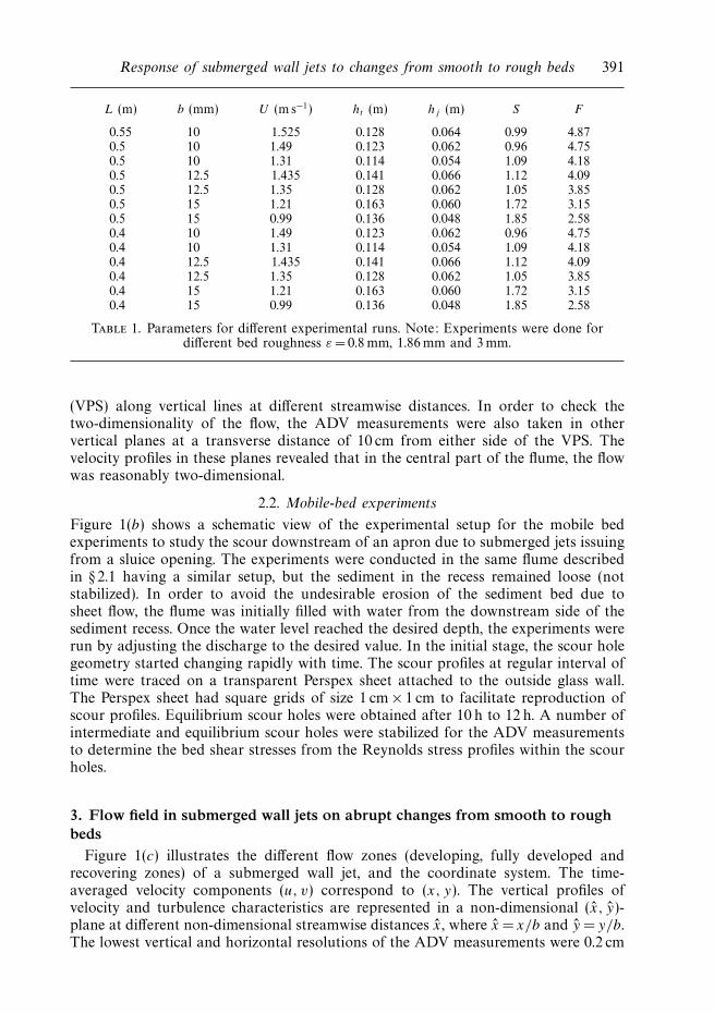
0.55 10 1.525 0.128 0.064 0.99 4.870.5 10 1.49 0.123 0.062 0.96 4.750.5 10 1.31 0.114 0.054 1.09 4.180.5 12.5 1.435 0.141 0.066 1.12 4.090.5 12.5 1.35 0.128 0.062 1.05 3.850.5 15 1.21 0.163 0.060 1.72 3.150.5 15 0.99 0.136 0.048 1.85 2.580.4 10 1.49 0.123 0.062 0.96 4.750.4 10 1.31 0.114 0.054 1.09 4.180.4 12.5 1.435 0.141 0.066 1.12 4.090.4 12.5 1.35 0.128 0.062 1.05 3.850.4 15 1.21 0.163 0.060 1.72 3.150.4 15 0.99 0.136 0.048 1.85 2.58

Table 1. Parameters for different experimental runs. Note: Experiments were done fordifferent bed roughness ε = 0.8 mm, 1.86mm and 3 mm.

(VPS) along vertical lines at different streamwise distances. In order to check thetwo-dimensionality of the flow, the ADV measurements were also taken in othervertical planes at a transverse distance of 10 cm from either side of the VPS. Thevelocity profiles in these planes revealed that in the central part of the flume, the flowwas reasonably two-dimensional.

2.2. Mobile-bed experiments

Figure 1(b) shows a schematic view of the experimental setup for the mobile bedexperiments to study the scour downstream of an apron due to submerged jets issuingfrom a sluice opening. The experiments were conducted in the same flume describedin § 2.1 having a similar setup, but the sediment in the recess remained loose (notstabilized). In order to avoid the undesirable erosion of the sediment bed due tosheet flow, the flume was initially filled with water from the downstream side of thesediment recess. Once the water level reached the desired depth, the experiments wererun by adjusting the discharge to the desired value. In the initial stage, the scour holegeometry started changing rapidly with time. The scour profiles at regular interval oftime were traced on a transparent Perspex sheet attached to the outside glass wall.The Perspex sheet had square grids of size 1 cm × 1 cm to facilitate reproduction ofscour profiles. Equilibrium scour holes were obtained after 10 h to 12 h. A number ofintermediate and equilibrium scour holes were stabilized for the ADV measurementsto determine the bed shear stresses from the Reynolds stress profiles within the scourholes.

3. Flow field in submerged wall jets on abrupt changes from smooth to roughbeds

Figure 1(c) illustrates the different flow zones (developing, fully developed andrecovering zones) of a submerged wall jet, and the coordinate system. The time-averaged velocity components (u, v) correspond to (x, y). The vertical profiles ofvelocity and turbulence characteristics are represented in a non-dimensional (x, y)-plane at different non-dimensional streamwise distances x, where x = x/b and y = y/b.The lowest vertical and horizontal resolutions of the ADV measurements were 0.2 cm


and 2 cm, respectively. In the following sections, figures 2–8 representing differentaspects of the flow field do not show all the experimental data at the lowest resolutionso as to avoid overlapping of profiles and data plots. In figures 2–8, the profiles ofvelocity and turbulence characteristics on rough beds are magnified using repre-sentative scales of the velocity and turbulence different from those on smooth beds.Smooth-bed data are shown by open symbols, and rough-bed data by filled symbols.In order to have a comparative study on the influence of the downstream roughbeds on the flow field, each of figures 2–8 shows three different runs for three roughbeds having identical length of smooth bed L, jet velocity U and sluice opening b.However, other runs are used to analyse the flow characteristics (figures 11–17).

3.1. Velocity profiles

The vertical profiles of non-dimensional time-averaged horizontal velocity componentu(= u/U ) at different streamwise distances x, in submerged wall jets on a rigid bedwith abrupt changes from smooth to rough beds, are shown in figure 2. The horizontalvelocity component u reveals the characteristics of the submerged wall jet issuing fromthe sluice over different flow zones, namely developing, fully developed and recoveringzones. The developing zone of the jet was close to the sluice opening. Hence, it wasnot always possible to detect the complete flow field in the developing zone dueto the ADV limitation. In figure 2, the upper and lower lines represent the loci ofu = 0 and the boundary layer in the submerged wall jets. It is observed that thelength of the fully developed zone, where u is reversal, decreases with increase in bedroughness ε for the same length L of the smooth bed. The positions of the maximumu in the individual profiles, show that the boundary layer grows more quickly in thepresence of the rough beds in general, and with increase in roughness in particular.This phenomenon is also obvious from the free-surface profiles. The most importantfeature to be noticed is the depression of the free-surface elevation and the variationof free-surface curvature in the developing and fully developed zones on the smoothbed with increase in bed roughness ε. This implies that the effect of the roughness ε

of a rough bed on the flow over a smooth bed is prominent. The reversal mode of u,in the fully developed zone, signifies an apparent surface roller (swirl flow), while inthe recovering zone, the flow is nearly horizontal.

The vertical profiles of non-dimensional time-averaged vertical velocity componentv(= v/U ) at different x, in submerged wall jets on a rigid bed with abrupt changesfrom smooth to rough beds, are presented in figure 3. It is shown that above the bedthe direction of v, being downward on the smooth bed, changes from downward toupward at the junction of the smooth and rough beds. This is due to the roller flowabove the expanding jet. From an observation of the flow fields, it is revealed that theupward motion of the flow increases with increase in roughness ε of the rough beds.Therefore, the frictional resistance exerted by the bed roughness on the submergedwall jet is distinguishable in the fully developed zone. In the profiles of v on thesmooth bed, it is evident that the effect of the bed roughness on the submerged walljet reduces the downward flow (see figure 3c).

Figure 4 depicts the non-dimensional velocity vectors in submerged wall jets ona rigid bed with abrupt changes from smooth to rough beds. The magnitude anddirection of velocity vectors are given by (u2 + v2)0.5 and arc tan(v/u), respectively.The characteristics of the decay of jet velocity including a roller flow in the fullydeveloped zone are obvious. Importantly, no noticeable discontinuity in the velocitydistributions is observed due to abrupt changes of bed roughness. The behaviour isdifferent from that observed in closed-conduit flows, where an overshooting property


0

3

6

9

12

15

y

0

3

6

9

12

15 30 45 60 75 90

x

0

3

6

9

12

–1 0 1

u

–0.5 0 0.5(a)

(b)

(c)

Smooth Rough

Smooth Rough

Smooth Rough

RZFDZ

RZFDZ

RZFDZ

ˆ

ˆ

y

y

ˆ

u

Figure 2. Vertical profiles of u for U =1.435m s−1, L = 0.4 m and b = 12.5mm: (a) ε = 0.8 mm,(b) ε = 1.86mm and (c) ε = 3 mm (FDZ and RZ refer to the fully developed and recoveringzones, respectively).

was reported (Antonia & Luxton 1971). A possible reason for this difference is thatwhen an open channel flow is subjected to an abrupt change of bed roughness, theflow field adjusts gradually through the change of free-surface profile (Chen & Chiew2003). Also, there was no step change due to roughness in the present case, whichmight be another reason.


0

3

6

9

12

15

y

0

3

6

9

12

15 30 45 60 75 900

3

6

9

12

–0.1 0 0.1

v

–0.05 0 0.05(a)

(b)

(c)

ˆ

ˆ v

y

y

x

Figure 3. Vertical profiles of v for U = 1.435m s−1, L =0.4 m and b = 12.5 mm:(a) ε = 0.8 mm, (b) ε = 1.86mm and (c) ε = 3 mm.

3.2. Turbulence intensity profiles

The vertical profiles of the non-dimensional horizontal turbulence intensity componentu+(= (u′u′)0.5/U , where u′ is the fluctuation of u) at different x, in submerged walljets on a rigid bed with abrupt changes from smooth to rough beds, are plotted infigure 5. Pronounced bulges in the profiles of u+ on the smooth bed are apparentas a result of reversed flow. On the rough beds, the profiles of u+ have continuity


0

3

6

9

12

15(a)

(b)

(c)

0.8UU

y

y

y

0

3

6

9

12

15 30 45 60 75 900

3

6

9

12

ˆ

ˆ

ˆ

x

Figure 4. Non-dimensional velocity vectors for U = 1.435m s−1, L = 0.4 m and b = 12.5 mm:(a) ε = 0.8 mm, (b) ε = 1.86mm and (c) ε = 3 mm.

(that is the change is gradual) with those of smooth bed, in the fully developed zone.On the other hand, in the recovering zone, u+ increases with increase in verticaldistance y over a short distance, then becoming almost constant over the entire zone.In the fully developed zone, u+ increases with increase in y, becoming maximumat approximately y = 0.5–0.6, and then decreases gradually with increase in y. Thelocal maximum value of u+ of a vertical profile increases initially with increase in


0

3

6

9

12

15

0

3

6

9

12

15 30 45 60 75 900

3

6

9

12

0 1

u+ u+

0 0.5(a)

(b)

(c)

y

y

y

x

Figure 5. Vertical profiles of u+ for U = 1.435m s−1, L = 0.4 m and b = 12.5 mm:(a) ε = 0.8 mm, (b) ε = 1.86mm and (c) ε = 3 mm.

streamwise distance x up to an overall maximum at the middle of the smooth bedand then decreases gradually towards the recovering zone on the rough beds.

Figure 6 shows the vertical profiles of non-dimensional vertical turbulence intensitycomponent v+(= (v′v′)0.5/U , where v′ is the fluctuation of v) at different x insubmerged wall jets on a rigid bed with abrupt changes from smooth to roughbeds. In the profiles of v+, bulges are evident at the mid flow depth except near the


0

3

6

9

12

15

0

3

6

9

12

15 30 45 60 75 900

3

6

9

12

0 0.25

v+ v+

0 0.13(a)

(b)

(c)

y

y

y

x

Figure 6. Vertical profiles of v+ for U = 1.435m s−1, L =0.4 m and b = 12.5 mm:(a) ε = 0.8 mm, (b) ε = 1.86mm and (c) ε = 3 mm.

sluice opening. The influence of roughness is prominent as, in the fully developed andrecovering zones, the magnitude of v+ of a particular profile increases with increase inroughness ε. However, v+ increases with increase in x up to the junction of the smoothand rough beds and then decreases to attain a constant profile in the recovering zone.

3.3. Decay of submerged wall jet

Figure 1(c) shows schematic profiles of the horizontal velocity component in a sub-merged wall jet. The local maximum jet velocity u0, which is the maximum velocity


of an individual vertical profile of u at any distance x, decreases with increase instreamwise distance x due to an increase in boundary layer thickness δ. In order torepresent the decay of a submerged wall jet in the streamwise direction due to abruptchanges from smooth to rough beds, the functional representations of the variations oflocal maximum velocity u0 and boundary layer thickness δ along streamwise distancex are given by

u0(x L) = u0(U, b, x, ν), u0(x > L) = u0(U, b, x − L, ε), (3.1a)

δ(x L) = δ(U, b, x, ν), δ(x > L) = δ(U, b, x − L, ε), (3.1b)

where ν is the kinematic viscosity of the fluid. Applying dimensional analysis, the non-dimensional equations for u0 and δ, whose coefficients and exponents were derivedby multiple linear regression analysis using all the experimental data collected by theADV, are.

u0(x L) = 1 − 0.235x0.4R−0.05, u0(x > L) = 1 − 0.1(x − L)0.55ε0.05, (3.2a)

δ(x L) = 0.27(x + 11.2)0.72R−0.2, δ(x > L) = 0.21(x − L)0.75ε0.25, (3.2b)

where u0 = u0/U , L =L/b, R is the Reynolds number of the issuing jet (= Ub/ν),ε = ε/b and δ = δ/b. Note that the term (x + 11.2), in (3.2 b), is important incomputation of the boundary layer thickness, because the virtual origin of theboundary layer of a jet is at x = −11.2 b where δ = 0 (Schwarz & Cosart 1961).Equations (3.2 a) and (3.2 b) indicate that the maximum jet velocity u0 diminishes andthe boundary layer thickness δ increases with increase in streamwise distance x.

4. Reynolds stress profiles4.1. Theoretical Reynolds stress

The two-dimensional Navier–Stokes equations of a steady turbulent flow are given innon-dimensional form (Rajaratnam 1976) as

u∂u

∂x+ v

∂u

∂y= −∂p

∂x+

1

R

(∂2u

∂x2+

∂2u

∂y2

)− ∂u+2

∂x− ∂uv+

∂y, (4.1)

u∂v

∂x+ v

∂v

∂y= −∂p

∂y+

1

R

(∂2v

∂x2+

∂2v

∂y2

)− ∂v+2

∂y− ∂uv+

∂x, (4.2)

where p = p/(ρU 2), p is the piezometric pressure, ρ is the mass density of fluidand uv+ is the non-dimensional Reynolds stress, that is -u′v′/U 2. The continuityequation is

∂u

∂x+

∂v

∂y= 0. (4.3)

Since u v, velocity and stress gradients in the y-direction are much greater thanthose in the x-direction. Thus, (4.2) becomes ∂p/∂y = −∂v+2/∂y (Townsend 1956;Rajaratnam 1976). Therefore, from (4.1) one can write

u∂u

∂x+ v

∂u

∂y+

∂

∂x(u+2 − v+2) +

∂uv+

∂y=

1

R

∂2u

∂y2. (4.4)

The general characteristic feature of the flow in submerged wall jets is self-preserving(see § 6). Therefore, the following functional relationships can be considered for thesolution of (4.4):

u = u0 ψ(η), u+2 = u20 φ1(η), v+2 = u2

0 φ2(η), uv+ = −u20 ξ (η), (4.5)


ε (mm) c α β σ

Smooth bed −1.41 7.81 1.308 0.6410.8 −1.12 5.42 1.048 0.4261.86 −0.93 5.05 0.862 0.4123 −0.9 4.95 0.642 0.397

Table 2. Values of coefficient and exponents in equations (4.8), (4.9) and (5.1).

where η = y/δ. Substituting (4.5) into (4.4), one obtains

δ

u0

∂u0

∂xψ2 − 1

u0

d(u0δ)

dx

dψ

dη

∫ η

0

ψdη + 2δ

u0

du0

dxφ1 − dδ

dxηdφ1

dη+

dδ

dxηdφ2

dη

− 2φ2

δ

u0

du0

dx− dξ

dη=

1

R

d2ψ

dη2. (4.6)

Inserting the functional relationships for ψ , φ1, φ2 and ξ given in (4.5) into (4.6) andthen integrating (neglecting the viscous term), the expression for the non-dimensionalReynolds stress uv+ is obtained as

uv+ = −u0δdu0

dx

∫ h

η

ψ2dη − u0

(δdu0

dx+ u0

dδ

dx

)(∫ h

η

ψ2dη + ψ

∫ η

0

ψdη

)(4.7)

where h = h/b and h is the flow depth at any x. From the similarity of the profilesof u at different streamwise distances x, one can determine ψ =ψ(η). Equations forψ are obtained from the least square fitting of all the experimental data in the fullydeveloped zone as

ψ(η 1) = η1/α, (4.8)

ψ(η > 1) = exp[c(η − 1)0.95], (4.9)

where α and c are the exponent and coefficient, respectively, being dependent onthe roughness ε of the beds. Table 2 furnishes the values of the exponent α and thecoefficient c for different ε. For flow on a smooth bed, the value of α is close to thatin a turbulent boundary layer, where it lies between 7 and 10 (Dey 2002). Using theexpressions for u0, δ and ψ in (4.7), profiles of uv+ are computed. Figure 7 shows thevertical profiles of computed uv+.

4.2. Experimental Reynolds stress

Figure 7 displays the vertical profiles of non-dimensional Reynolds stress uv+ atdifferent x in submerged wall jets on a rigid bed with abrupt changes from smoothto rough beds. The Reynolds stress uv+ near the bed is positive and reduces sharply,changing its sign to negative and forming weak bulges (maximum negative valueof uv+ in a vertical profile) with increase in vertical distance y due to the surfaceroller on the smooth bed. The bulges in the profiles of uv+ gradually disappear withincrease in x, especially on the rough beds. However, in the recovering zone, as uv+

is weak (in comparison with uv+ in the fully developed zone) it is almost constantalong the vertical. It is apparent from the comparison between the experimental dataand computed profiles of uv+, in figure 7, that there is a difference in the data insome profiles in the recovering zone. This is attributed to uv+ being computed from


0

3

6

9

12

15

0

3

6

9

12

15 30 45 60 75 900

3

6

9

12

–0.1 0 00.1

uv+ uv+

–0.05 0.05(a)

(b)

(c)

Equation (4.7)

y

y

y

x

Figure 7. Vertical profiles of Reynolds stress uv+ for U = 1.435m s−1, L =0.4 m andb = 12.5 mm: (a) ε =0.8 mm, (b) ε = 1.86mm and (c) ε =3 mm.

(4.7), which is dependent on u0, δ and ψ determined empirically (see 3.2(a), 3.2(b),(4.8) and (4.9)) from experimental data that are independent of the experimental datafor uv+. In addition, having used a number of empirically determined parameters, aperfect matching between the experimental data and the computed results is diffi-cult. However, the computed profiles of uv+ agree reasonably with the experimentaldata.


5. Bed shear stress5.1. Theoretical bed shear stress

Inserting (4.3) and (4.5) into (4.4) and integrating the resulting equation, the followingexpression for the non-dimensional bed shear stress is obtained:

τ = −(

2δu0

du0

dx+ u2

0

dδ

dx

)∫ η

0

(ψ2 + φ1 − φ2) dη (5.1)

where τ = τ/(ρU 2). To solve (5.1), one requires information on φ1(η) and φ2(η).Therefore, the expressions for φ1 = η1/β and φ2 = η1/σ are obtained from least-squarefitting of the present experimental data. The exponents β and σ are functions ofbed roughness ε. Table 2 furnishes the values of exponents β and σ for different ε

determined from the least-square fitting of all the experimental data in the fully deve-loped zone. The bed shear stress τ is computed from (5.1), using the expressions foru0, δ, ψ , φ1 and φ2. The computed horizontal distributions of τ are shown in figure 8.

5.2. Experimental bed shear stress

Experimental values of the bed shear stress τ are estimated from the Reynolds stressprofiles extending on to the bed level, as was done by Dey & Lambert (2005). Thenon-dimensional bed shear stress is, therefore, given by

τ = uv+|η=0. (5.2)

Figure 8 shows the distributions of non-dimensional bed shear stress τ along stream-wise direction x. Bed shear stress τ decreases with increase in streamwise distance x;and the change in τ at the junction of smooth and rough beds is basically gradual,though a slight discontinuity is observed in the computed curves. It is evident from thecomparison of the experimental data and computed curves that there is a tendencyto overestimate the bed shear stress. The discrepancy between the experimental andthe computed values of τ results from the experimental scatter. It may be noted thatτ is determined from the Reynolds stress profiles, which are sensitive to the turbulentfluctuations and hence subject to uncertain attenuation and error, especially near thebed. Nevertheless, in general, collapse of the experimental data and the computedcurves is reasonable on rough beds.

6. Flow characteristics of submerged wall jets over abrupt changes fromsmooth to rough beds

6.1. Determination of length scale

For the local maximum jet velocity u0, the length scale λ, which groups the data of allmajor flow characteristics, is the distance from the sluice opening at which u0 =U/2.Long et al. (1990) used the following relationship for λ for smooth bed:

λ

b=

49

1 + C1(dh/dx)λF −2(6.1)

where C1 is a coefficient. For the combination of smooth and rough beds, the free-surface slope, that is (dh/dx)λ, at x = λ is a function of S, L and ε, as shown infigures 9(a) and 9(b). Using the least-square curve fitting, the following relationshipfor different L and ε is obtained:(

dh

dx

)λ

= C2 × 10−KS (6.2)


0

1

2

3

ˆ

4

τ (×

103 )

τ (×

103 )

τ (×

103 )

0

1

2

3

4

15 30 45ˆ

60 75 90x

0

1

2

3

4

Smooth bed

Observed

Equation (5.1)

Rough bed

Observed

Equation (5.1)

(a)

(b)

(c)

Figure 8. Horizontal distributions of bed shear stress τ for U = 1.435m s−1, L = 0.4 m andb = 12.5 mm: (a) ε = 0.8 mm, (b) ε = 1.86 mm and (c) ε = 3 mm.

where C2 and K are the coefficients and exponents, respectively, being dependent onL and ε. Substituting (6.2) in (6.1), one can write

λ

b=

49

1 + C × 10−KSF −2(6.3)

where coefficient C is the product of C1 and C2. The values of C for different L and ε

are determined from the least-square curve fitting of the plots of λ/b versus 10−KSF −2

as shown in figures 9(c) and 9(d). The dependence of C and K on relative roughnessε for different L is given in figures 9(e) and 9(f ), respectively.

Barring the horizontal length scale λ, the vertical length scale y1 for velocity u,shown in figure 10(a), is used to collapse the vertical distributions of u onto a singleband. It is the vertical distance y where u = u0/2 and ∂u/∂y < 0. Moreover, the verticallength scale y2 for the Reynolds stress −u′v′, shown in figure 10(b), being the vertical


1 2 3 1 2 3S

0

0.05

0.10(a) (b)

(d)

( f )

(c)

(e)

(dh

/dx)

λ

0 0.05 0.050.10 0 0.10

10–KS F –2 10–KS F –2

20

30

40

λ

S0

0.05

0.10

20

30

40

0.3

0.6

K

0.2 0.40 0.2 0.40ˆ

25

50

C

(mm)ε

ε ε

0.8

1.86

3

L = 0.4 m

L = 0.5 m

L = 0.4 m

L = 0.5 m

b

Figure 9. (a) (dh/dx)λ as a function of S for L = 0.4 m, (b) (dh/dx)λ as a function of S forL = 0.5 m, (c) λ/b as a function of 10−KSF −2 for L = 0.4 m, (d) λ/b as a function of 10−KSF −2

for L = 0.5 m, (e) variation of C with ε and (f ) variation of K with ε.

distance y where u′v′ = (u′v′)0/2 and ∂(u′v′)/∂y < 0, is considered to group the verticaldistributions of uv+ together. Subscript 0 refers to a local maximum value in a verticalprofile. Furthermore, for the null-point of the Reynolds stress profiles, y = δ1 whereu′v′ = 0 and ∂(u′v′)/∂y > 0.


u0

y

u

u0/2

δ

δ1

y1

(a) (b)

y

–(u′v′)0/2

–(u′v′)0

–u′v′

y2

Figure 10. (a) Schematic velocity profile and (b) schematic Reynolds stress profile.

6.2. Flow characteristics

The decay of non-dimensional maximum velocity u0/U , in the fully developed zone,over non-dimensional streamwise distance x(= x/λ) in a submerged wall jets over anabrupt change from smooth to rough beds having different roughness ε, is representedin figure 11(a) for the smooth bed length L =0.5 m. Different symbols are used torepresent the data for smooth and rough beds. The use of a common length scaleλ for the flow over smooth and rough beds, makes it possible for all the data tocollapse reasonably on a single band (which means that the data have a definite meantrend), though in the vicinity of the junction of the smooth and rough beds (x 1)a little data scatter exists due to the abrupt changes of bed roughness. To be moreexplicit, the abrupt change of bed roughness reduces the magnitude of maximumvelocity u0 drastically due to the additional resistance resulting in a locally dispersedtrend. However, the effect of the bed roughness is also noticeable from the free-surface profiles (see figure 4), as there is a considerable depression of the free-surfaceelevation over the smooth bed with increasing bed roughness. A comparative studyof the present data trend with the curves of a wall jet (Rajaratnam 1976), free jump(Rajaratnam 1965) and submerged jet on a smooth bed (Long et al. 1990) revealsthat the mean trend of u0/U versus x data for submerged wall jets on a smoothbed coincides with the curves of a free jump and a submerged jet on a smooth bed.However, upstream of the junction of smooth and rough beds, the data trend differ.All the data of a rough bed lie well below the curves of a free jump and submergedjet on smooth bed. Hence, one can conclude that the decay rate of local maximumvelocity u0, being significantly influenced by the bed roughness ε, increases on roughbeds; and the flow is self-preserving on smooth and rough beds. It is revealed fromdata not shown (to restrict the number of figures) for L = 0.4mm that a decreaseof the length L of the smooth bed expedites the decay rate for obvious reasons.Importantly, the use of the same length scale λ also makes it possible to collapse thedata of (uv+)0/(uv+)m, (u+)0/(u+)m and (v+)0/(v+)m approximately onto a single band,as shown in figures 11(b), 12(a) and 12(b), respectively, though as usual there is a littledata scatter in the vicinity of the junction of smooth and rough beds. Here, subscriptm refers to a maximum for an experimental condition. The comparisons show thatthe present data trends have good agreement with the curve of a submerged jet on asmooth bed in the smooth bed region, but they lie below the curve of a submergedjet on smooth bed in the rough bed region due to the roughness effect. Therefore,


0

0.4

0.8

1.2

u0

Wall jet

Free jump

(a)

(b)

Submerged jet on smooth bed

Smooth Rough

0.8

1.86

3

1 2 3 4

1 2 3 4

x~0

0.4

0.8

1.2

(uv+

) 0/(

uv+)m


U

ε (mm)

Figure 11. (a) u0/U as a function of x and (b) dependence of (uv+)0/(uv+)m on x, fordifferent ε and L = 0.5m.

the rates of decay of (uv+)0, (u+)0 and (v+)0 on rough beds are faster than those onsmooth beds, as a result of mixing of fluid caused by the roughness.

To assess the degree of similarity in the individual profiles of u in the fully developedzone, using u0 and y1 as the scales, the profiles of non-dimensional horizontal velocityu/u0 are plotted against non-dimensional vertical distance y (= y/y1) in figures 13(a)and 13(b) for smooth and rough bed regions, respectively. In figure 13(a), the collapseof the velocity data and the curves for the wall jet and submerged jet on smoothbed is good up to y = 1.5 for different downstream roughness ε. The velocity datadepart from the wall jet curve in the outer layer for y > 1.5. The negative magnitudeof u/u0 in the outer-layer profiles indicates the region of reversed flow. In the upperportion of the outer layer, the mean data trend lies between the curves of the wall jetand submerged jet on smooth bed. For the flow on a rough bed, the profiles of u/u0,in the inner layer, are influenced by the bed roughness (see figure 13b). In reality,the bed roughness increases the inner-layer thickness of individual velocity profiles.Hence, the rough bed data near the bed are less ‘full’ compared to the curves ofthe wall jet and submerged jet on the smooth bed. The data of uv+/(uv+)0 versus ζ

(= (y − δ1)/(y2 − δ1)), u+/(u+)0 versus z(= y/y2) and v+/(u+)0 versus z are plotted infigures 14–16 illustrating the degrees of similarity that exist in the individual profiles


0.4

0.8

1.2

(u+)0

(a)

(b)


Smooth Rough ε (mm)

0.8

1.86

3

1 2 3 4

x~0

1 2 3 40

0.4

0.8

1.2


(u+)m

(v+)0

(v+)m

Figure 12. (a) Dependence of (u+)0/(u+)m and (b) dependence of (v+)0/(v

+)m on x fordifferent ε and L =0.5m.

of uv+, u+ and v+ in the fully developed zone on smooth and rough beds. The dataof smooth bed regions and the curves of the submerged jet on a smooth bed collapsein the inner layer (figures 14a, 15a and 16a). On the other hand, as a result ofincreasing turbulence intensity on account of the roughness, the data of (u+)0 and(v+)0 of rough bed regions lie in between the curves of wall jet and submerged jeton a smooth bed in the inner layer (figures 14b and 15b); whereas the data of (uv+)0of rough bed regions (figure 16b), being sagging in nature, intercept wall jet curve atζ = 0.05. However, in the outer layer, the data of smooth and rough bed regions arecloser to the curves of the wall jet. To be more explicit, the roughness ε augments theinner-layer thickness of the u+ and v+ profiles.

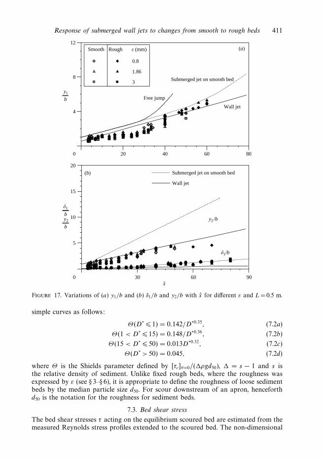
The streamwise variations of non-dimensional vertical length scale y1/b for hori-zontal velocity component u are shown in figure 17(a) for L =0.5 m. It shows thatthe jet half-widths on smooth and rough beds decay slower and faster than that in aclassical wall jet, respectively. Therefore, the jet half-width is influenced significantlyby an abrupt change of bed roughness. However, the data lie well below the curves of


–0.5

0

0.5

1.0

1.5

uu0

(a)

(b)

L = 0.4 m L = 0.5 m ε (mm)

0.8

1.86

3


Wall jet

0 2 4 6 8

0 2 4 6 8

y~

–0.5

0

0.5

1.0

1.5

uu0

Figure 13. (a) u/u0 as a function of y in fully developed zone of smooth beds for differentdownstream ε and L (L =0.4m (data range: 3.3 x 20) and 0.5m (data range: 3.3 x 26.7)) and (b) u/u0 as a function of y in fully developed zone of rough beds for different εand upstream L (L =0.4m (data range: 26.7 x 40) and 0.5m (data range: 33.3 x 40)).

a free jump and submerged jet on a smooth bed. Figure 17(b) presents the change ofy2/b with x, which is the decay of half-widths of the Reynolds stress in the streamwisedirection. The half-widths of the Reynolds stress on smooth and rough beds decaysslower than those in the wall jet and submerged jet on smooth bed. It is seen from theplot of δ1/b versus x, in figure 17(b), that the null-points of the Reynolds stress profilesin smooth and rough beds remain similar to those in a submerged jet on a smooth bed.

7. Modelling of scour downstream of an apron7.1. Experimental observation on the scour process

The scouring process downstream of an apron due to submerged jets issuing froma sluice opening is a multifaceted phenomenon owing to the abrupt change of


–0.4 0 0.4 0.8 1.2 1.6 2.0

–0.4 0 0.4 0.8ζ

1.2 1.6 2.0

–0.4

0

0.4

0.8

1.2

uv+/(

uv+) 0

uv+/(

uv+) 0

(a) L = 0.4 m L = 0.5 m ε (mm)

0.8

1.86

3


Wall jet

–0.4

0

0.4

0.8

1.2(b)

Figure 14. (a) Similarity of distributions of uv+ in fully developed zone of smooth beds fordifferent downstream ε and L (L =0.4m (data range: 3.3 x 20) and 0.5m (data range:3.3 x 26.7)) and (b) similarity of distributions of uv+ in fully developed zone of roughbeds for different ε and L (L = 0.4m (data range: 26.7 x 40) and 0.5m (data range:33.3 x 40)).

the flow characteristics (including free-surface profile) on the sediment bed with time(figure 18a). The sediment bed following a smooth rigid apron of length L was initiallyplanar and the submerged jet flowed in a direction parallel to the bed surface. It isimportant to mention that the increased depression of the free surface in the presenceof the sediment bed (that is the rough bed) downstream of an apron, apparent infigure 4, enhanced the erosive power of the submerged jet. Scour starts at the down-stream edge of the apron when the bed shear stress induced by the submerged wall jetexceeds the threshold bed shear stress for sediment movement. The evolution of thevertical dimension of the scour hole was faster than the longitudinal one. In the initialstage, the suspension of sediment, in addition to the bed-load, was the main means ofsediment transport. But with the increase of the vertical dimension of the scour hole,the mode of sediment transport changed to bed-load only. The down-slope sliding androlling movement of sediment took place when the bed shear stress induced by thesubmerged wall jet was reduced considerably with the development of the scour hole.


0.4 0.8 1.2 1.6 2.00

0.4 0.8 1.2 1.6 2.0

0.3

0.6

0.9

1.2

(u+)0

(a)

(b)

L = 0.4 m L = 0.5 m ε (mm)

0.8

1.86

3


Wall jet

z0

0.3

0.6

0.9

1.2


Wall jet

u+

(u+)0

u+

Figure 15. (a) Similarity of distributions of u+ in fully developed zone of smooth beds fordifferent downstream ε and L (L =0.4m (data range: 3.3 x 20) and 0.5m (data range:3.3 x 26.7)) and (b) similarity of distributions of u+ in fully developed zone of roughbeds for different ε and L (L =0.4 m (data range: 26.7 x 40) and 0.5m (data range:33.3 x 40)).

The upstream side of the scour hole achieved a steeper slope than the downstreamside. However, after a considerable period of time, equilibrium was reached, whenthe sediment particles at the surface of the scour hole remained at the thresholdcondition.

7.2. Equilibrium of sediment particles

The forces acting on a sediment particle lying on the equilibrium scoured bed, shownin figure 18(a), are the drag force FD , lift force FL, and submerged weight of asediment particle FG. Based on these forces, the threshold condition of a sedimentparticle resting on a bed slope θ (streamwise) can be defined by the following equation:

τc = cos θ

(1 +

tan θ

µ

)(7.1)

where τc = [τc]θ=θ /[τc]θ=0, θ = arc tan(dy/dx), µ is the Coulomb frictional coefficientof sediment, equalling tanφ, and φ is the angle of repose of sediment. Subscript ‘c’


0.4 0.8 1.2 1.6 2.0

0.4 0.8 1.2 1.6 2.0

0

0.3

0.6

0.9

1.2

(a)

(b)

L = 0.4 m L = 0.5 m ε (mm)

0.8

1.86

3


Wall jet

z0

0.3

0.6

0.9

1.2Submerged jet on smooth bed

Wall jet

(u+)0

v+

(u+)0

v+

Figure 16. (a) Similarity of distributions of v+ in fully developed zone of smooth beds fordifferent downstream ε and L (L =0.4m (data range: 3.3 x 20) and 0.5m (data range:3.3 x 26.7)) and (b) similarity of distributions of v+ in fully developed zone of roughbeds for different ε and L (L = 0.4m (data range: 26.7 x 40) and 0.5m (data range:33.3 x 40)).

refers to the threshold or critical condition. The threshold bed shear stress [τc]θ=0

for uniform sediment on a horizontal bed (θ = 0) can be obtained mathematicallyfrom the model given by Dey (1999). The most accurate curve for the determinationof threshold bed shear stress was given by Yalin & Karahan (1979). It is very closeto the results obtained from the model of Dey (1999). The representation of theShields parameter and the shear Reynolds number in a single curve, as was done byShields, requires trial-and-error to solve the bed shear stress or shear velocity, as bedshear stress and shear velocity, being interchangeable, are dependent and independentvariables. To avoid this difficulty, the Shields parameter is represented as a function ofthe particle parameter D∗[= d50(g/ν2)1/3] (Dey, Dey Sarker & Debnath 1999; Dey1999). Importantly, D∗ does not involve different bed categories. However, the curveproposed by Dey (1999) for the sediment threshold can be expressed by a number of


20 40 60 800

4

8

12

y1

(a)

(b)

Smooth Rough ε (mm)

0.8

1.86

3 Submerged jet on smooth bed

Free jump

Wall jet

30 60 90x

0

5

10

15

20

y2 /b

δ1/b


Wall jet

b

y2

b

δ1

b

ˆ

Figure 17. Variations of (a) y1/b and (b) δ1/b and y2/b with x for different ε and L = 0.5 m.

simple curves as follows:

Θ(D∗ 1) = 0.142/D∗0.35, (7.2a)

Θ(1 < D∗ 15) = 0.148/D∗0.36, (7.2b)

Θ(15 < D∗ 50) = 0.013D∗0.32, (7.2c)

Θ(D∗ > 50) = 0.045, (7.2d)

where Θ is the Shields parameter defined by [τc]θ=0/(ρgd50), = s − 1 and s isthe relative density of sediment. Unlike fixed rough beds, where the roughness wasexpressed by ε (see § 3–§ 6), it is appropriate to define the roughness of loose sedimentbeds by the median particle size d50. For scour downstream of an apron, henceforthd50 is the notation for the roughness for sediment beds.

7.3. Bed shear stress

The bed shear stresses τ acting on the equilibrium scoured bed are estimated from themeasured Reynolds stress profiles extended to the scoured bed. The non-dimensional


45 ˆ90 135x

y

0

ˆ

1

τ (×

103 )

–8

0

8

16

Bed shear stress

Observed

Threshold

Equation (7.4)

Scour hole

Dune

Apron

Dune

Tailwater level

x

y

b

Sluice gate

Apron

Sediment bed

0

(a)

(b)

FL

FG

FDθ

dst

L

Figure 18. (a) Schematic diagram of scour downstream of an apron due to a submerged jetissuing from a sluice opening and (b) variations of bed shear stress τ on scoured beds forU = 1.435m s−1, L =0.4m, b = 12.5mm and d50 = 0.8 mm.

bed shear stress [τ ]θ=θ at any location on the scoured bed with local angle θ is givenby

[τ ]θ=θ = τ cos θ. (7.3)

In figure 18(b), a comparison of the experimental bed shear stress and local thres-hold bed shear stress, obtained from (7.1) as [τc]θ=θ = [τc]θ=0 cos θ[1 + (tan θ/µ)],shows that the surface of the equilibrium scour hole is at threshold condition. (Note:to determine [τc]θ=θ for a given d50, D

∗ was calculated. Then, Θ was estimated from theset (7.2), and [τc]θ=0 from Θ(ρgd50). Thus, one can calculate [τc]θ=θ as [τc]θ=0/(ρU 2).)It is assumed that the bed shear stress for the two-dimensional submerged wall jeton scoured bed is equivalent to that for the two-dimensional submerged wall jet on asmooth bed followed by a rigid rough bed given by (5.1). This assumption leads to theapproximation that the bed profile does not influence the self-preserving characteristicsof the submerged wall jet, or alternatively, the aspect ratio of the scoured bed is small.In addition, the flow close to the bed is assumed to be not separated from the scouredbed, as was assumed by Hogg et al. (1997). However, this assumption may be inaptnear the upstream slope of the scour hole and downstream of the dune, where the


c0 c1 c2 c3 c4d50

(mm) y 0 y > 0 y 0 y > 0 y 0 y > 0 y 0 y > 0 y 0 y > 0 n

0.8 50.4 0.91 −2.965 −0.12 0.0611 1.8 × 10−3 −5 × 10−4 −2 × 10−6 1.5 × 10−6 0 0.141.86 49.4 1.27 −2.965 −0.16 0.0611 2.6 × 10−3 −5 × 10−4 −2.8 × 10−6 1.7 × 10−6 0 0.153 50.8 1.64 −2.965 −0.2 0.0611 3.3 × 10−3 −5 × 10−4 −3.6 × 10−6 1.6 × 10−6 0 0.16

Table 3. Values of coefficients in equation (7.6) for different d50.

flow separates. Nevertheless, it simplifies the problem considerably. Thus, one canhypothesize the bed shear stress on the equilibrium scoured bed to be

[τ ]θ=θ (x L) = −Ξ (x − L, y)

[(2δu0

du0

dx+ u2

0

dδ

dx

)∫ η

0

(ψ2 + φ1 − φ2) dη

]. (7.4)

The function Ξ , determined empirically using the bed shear stress obtained fromthe measured Reynolds stress profiles within the equilibrium scour holes, is given by

Ξ = 0.0081c4y/δ + 0.04(cy/δ)2. (7.5)

The parameter c in the above equation, being a function of x and d50, can be givenby the following polynomial:

c = c0 + c1(x − L) + c2(x − L)2 + c3(x − L)3 + c4(x − L)4. (7.6)

The values of coefficients c0, c1, c2, c3 and c4 for different d50 are given in table 3.Figure 18(b) shows that the bed shear stresses computed from (7.4), being tuned bythe experimental data, compare reasonably with those determined from the Reynoldsstress within the scour hole.

7.4. Profiles of equilibrium scour hole

The profile of the equilibrium scour hole can be computed from the threshold condi-tion of sediment particles resting on the surface of the scour hole under the bed shearstress distribution given by (7.4). This concept has been commonly used, such as todetermine the scour profiles below pipelines (Li & Cheng 1999, 2001). Using (7.1)and (7.4), the threshold condition of a sediment particle resting on the surface of thescour hole is given by

−Ξ (x − L, y)

[(2δu0

du0

dx+ u2

0

dδ

dx

)∫ η

0

(ψ2 + φ1 − φ2) dη

] [τc]θ=0 cos θ

(1 +

tan θ

µ

).

(7.7)

For the limiting equilibrium, (7.7) can be expressed as the following differentialequation:

(Ω2 − 1)dy

dx= µ ± [µ2 − (Ω2 − 1)(Ω2 − µ2]0.5 (7.8)

where

Ω = −0.0081c4y/δ + 0.04(cy/δ)2

[τc]θ=0

[(2δu0

du0

dx+ u2

0

dδ

dx

)∫ η

0

(ψ2 + φ1 − φ2) dη

]. (7.9)

Equation (7.8) is a first-order differential equation, which can be solved numericallyby the forth-order Runge–Kutta method to determine the variation of y with x,


0 30 60 90 120 150

0 30 60 90 120 150

0 30 60 90 120 150

–4

–2

0ˆ

2

4

y

y

y

x

–4

–2

0

2

4

–4

–2

0

2

4

Apron

Apron

Apron

Observed

Equation (7.8)

U = 0.99 m s–1

b = 15 mmL = 0.5 md50 = 0.8 mm

U = 1.21 m s–1

b = 15 mmL = 0.5 md50 = 1.86 mm

U = 0.99 m s–1

b = 15 mmL = 0.4 md50 = 3 mm

Original bed level

Original bed level

Original bed level

Figure 19. Comparisons of computed and experimental scour profiles.

that is the non-dimensional profile of an equilibrium scour hole. In (7.8) positiveand negative signs are associated with the solution for scour hole (y 0) and dune(y > 0) parts, respectively. In the present analysis, the value of µ was assumed to be0.65. From the experimental profiles, it was observed that the sediments at the edgeof the apron were washed away, as a result of which a small vertical portion of apron,of depth 0.35b, was exposed (Dey & Sarkar 2006). Therefore, (7.8) was solved for theinitial values of x = L and y = 0.35. Figure 19 shows the non-dimensional profilesof the equilibrium scour hole. The collapse of the computed and the experimentalprofiles is good within the scour hole. However, over the dune, the disagreement isdue to the flow separation at the crest of the dune.


7.5. Time variation of maximum scour depth

A simple model for the time variation of maximum scour depth (that is the maximumdepression of the bed level for an instantaneous scour hole profile) downstream ofan apron due to submerged wall jets is developed. It is based on the followingassumptions:

(i) the bed shear stress induced by the submerged wall jets is the main agent ofscouring, picking up the sediment particles from the beds;

(ii) the rate of change of sediment mass at the location (infinitesimal area) of themaximum scour depth equals the sediment mass removal rate from that location.

In a small interval of time dt , the sediment mass picked up from the location ofthe maximum scour depth of small width x is given by

dm1 = xEdt (7.10)

where E is the sediment pick-up rate at the location of the maximum scour depth attime t . During scouring at the location of the maximum scour depth, estimated usingthe equation of van Rijn (1984), it is

E = 0.00033ρs(gd50)0.5D∗0.3T 1.5 (7.11)

where ρs is the mass density of sediment and T is the transport-stage parameterdue to scouring, that is ([τ ]0 − [τc]θ=0)/[τc]θ=0 and [τ ]0 is the bed shear stress at thelocation of the maximum scour depth, being time dependent. This time-dependentbed shear stress [τ ]0 can be hypothesized using an exponential function dependenton instantaneous scour depth dst as follows:

[τ ]0 = − exp[−(C0dst )n]

[(2δu0

du0

dx+ u2

0

dδ

dx

)∫ η

0

(ψ2 + φ1 − φ2) dη

](7.12)

where C0 is the function of a parameter that defines the mobility of the sedimentparticles during scour and dst = dst/b. Dey & Sarkar (2006) recognized that thedensimetric Froude number F (= U/(gd50)

0.5) is the appropriate parameter whichdefines the mobility of the sediment particles. Here, in equilibrium profiles, thehorizontal location of the maximum scour depth is approximately x = L + 20. Fromthe comparison of the bed shear stress results on horizontal beds and equilibriumscoured beds, it is observed that the value of the bed shear stress does not vary muchfrom x = L to x = L+20. Therefore, in the calculation of [τ ]0 from (7.12), x = L+10can be considered as an average length. Using the bed shear stresses obtained fromthe measured Reynolds stress profiles at the locations of the maximum scour depthof intermediate and equilibrium scour holes, the equation for C0 and the values of n

are determined empirically: C0 = 0.02 exp(1.09F ); and the values of n for differentd50 are furnished in table 3.

The depletion of sediment mass due to an increase in scour depth ddst in time dt is

dm2 = −(1 − ρ0)ρsxddst (7.13)

where ρ0 is the porosity of the sediment. In this analysis, the value of porosityρ0 assumed was 0.4. From the concept of conservation of mass of sediment, thefundamental equation to describe the scouring process can be obtained as

dm1 + dm2 = 0. (7.14)

Equations (7.10) and (7.13) are substituted into (7.14) to obtain the followingdifferential equation of the time variation of maximum scour depth in non-dimensional


0

2

4

6

101 102 103 104 105 101 102 103 104 105

101 102 103 104 105 101 102 103 104 105

101 102 103 104 105 101 102 103 104 105

0

2

4

ˆ

6

dst

dst

dst

t

0

2

4

6

t

0

2

4

6

0

2

4

6

0

2

4

6

ˆ ˆ

t tˆ ˆ

U = 0.99 m s–1

b = 15 mmL = 0.5 md50 = 0.8 mm

U = 1.21 m s–1

b = 15 mmL = 0.5 md50 = 1.86 mm

U = 0.846 m s–1

b = 5 mmL = 0d50 = 2 mm

U = 1.21 m s–1

b = 15 mmL = 0.4 md50 = 0.8 mm

U = 1.31 m s–1

b = 10 mmL = 0.5 md50 = 3 mm

U = 0.843 m s–1

b = 5 mmL = 0.1 md50 = 2 mm

Present study

Equation (7.15)

(a)

(b)

Hopfinger et al. (2004)

Equation (7.15)

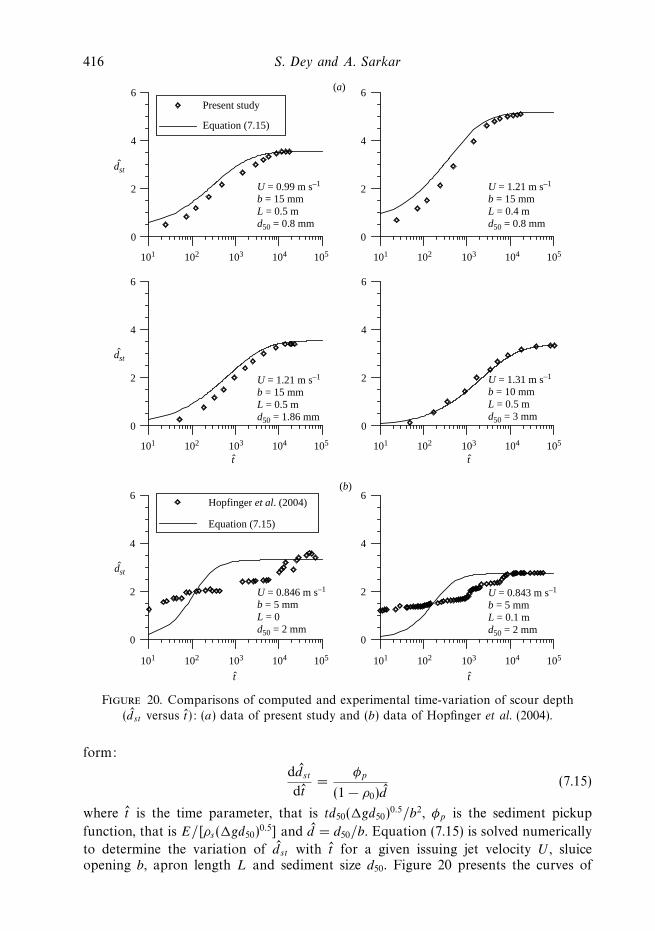
Figure 20. Comparisons of computed and experimental time-variation of scour depth

(dst versus t): (a) data of present study and (b) data of Hopfinger et al. (2004).

form:

ddst

dt=

φp

(1 − ρ0)d(7.15)

where t is the time parameter, that is td50(gd50)0.5/b2, φp is the sediment pickup

function, that is E/[ρs(gd50)0.5] and d = d50/b. Equation (7.15) is solved numerically

to determine the variation of dst with t for a given issuing jet velocity U , sluiceopening b, apron length L and sediment size d50. Figure 20 presents the curves of


non-dimensional time variation of scour depth. The collapse of the computed resultsand the experimental data of the present study, in figure 20(a), is satisfactory. However,there exists a considerable departure of the computed curves from the experimentaldata of Hopfinger et al. (2004) (figure 20b). Because Hopfinger et al. (2004) conductedthe experiments either without an apron or with a short apron, where the issuing jetsimmediately encountered the sediment beds (while in the present study, the jet travelsover an apron for a considerable distance before it encounters the sediment beds)there was a huge volume scour during the initial period, which is clearly evident fromfigure 20(b). (Note: as Hogg et al.’s (1997) model does not account the apron lengthL, it is thus applicable to the experiments of Hopfinger et al. (2004).) Importantly, thepresent model is developed for minimum length of the apron L = 0.5(b − hj), whichis the minimum dimension of the apron used in practice for dissipating the energy ofsubmerged jets. Thus, Hogg et al.’s (1997) model is limited in its applicability to thescour downstream of an apron, whereas the present model, which is the outcome ofa fundamental study of a submerged jets on an abrupt change from smooth to roughbeds, is applicable.

8. ConclusionsThe flow field for the decay of jet velocity in submerged wall jets over abrupt

changes from smooth to rough beds suggests that the decay rate of the jet is faster onrough beds. Hence, the growth of the boundary layer is quicker with an increase inbed roughness. The change in bed roughness induces an increased depression of thefree surface over the smooth bed (figure 2). The Reynolds and bed shear stresses havebeen determined from the solution of the Navier–Stokes equations. The variations offlow, turbulence and stress characteristics of submerged wall jets at the junction ofsmooth and rough beds are gradual (figures 2–8). The response of the turbulent flowcharacteristics of submerged wall jets to abrupt changes from smooth to rough bedshas been analysed from the point of view of similarity, growth of the length scale anddecay of the velocity and turbulence characteristics scales. As there is no step changeof roughness, use of a common length scale collapses the velocity and turbulencedata to a single band (figures 11 and 12). The flow is mainly self-preserving on bothsmooth and rough beds, though in the vicinity of their junction a little data scatterexists. The decay rates of local maximum horizontal velocity component, Reynoldsstress, horizontal and vertical turbulence intensity components on rough beds arefaster than those on smooth beds, as a result of the mixing of fluid due to roughness(figures 11 and 12). The inner-layer thickness of the horizontal velocity componentand the turbulence intensity profiles on rough beds increases with bed roughness(figures 13–16). On smooth beds, in general, the velocity and turbulence intensitydistributions collapse onto the corresponding curves of submerged jets on smoothbeds (figures 13a–16a). But on rough beds, they depart from the corresponding curvesof submerged jets on smooth beds (figures 13b–16b). The jet half-widths on smoothand rough beds decay slower and faster than that in classical wall jets, respectively(figure 17a). On the other hand, the half-width of the Reynolds stresses on smoothand rough beds decays slower than those in the wall jets and submerged jets onsmooth beds (figure 17b). However, the null-points of the Reynolds stress profileson smooth and rough beds remain same as that in submerged jets on smooth beds(figure 17b).

The profiles of the equilibrium scour hole have been calculated from the thresholdcondition of the sediment particles along the bed surface. The modification of the bed


shear stress expression due the variation of downstream scour profile has permittedthe computation of equilibrium profiles of the scour holes (figure 19). The timevariation of maximum scour depth has also been estimated using the bed shear stressexpression modified by an exponential function for the time dependence (figure 20).The collapse of the results obtained from the model and the present experimentaldata is satisfactory (figures 19 and 20).

REFERENCES

Antonia, R. A. & Luxton, R. E. 1971 The response of a turbulent boundary layer to a step changein surface roughness. Part 1. Smooth to rough. J. Fluid Mech. 48, 721–761.

Chatterjee, S. S. & Ghosh, S. N. 1980 Submerged horizontal jet over erodible bed. J. Hydr. Div.ASCE 106, 1765–1782.

Chen, X. & Chiew, Y. M. 2003 Response of velocity and turbulence to sudden change of bedroughness in open-channel flow. J. Hydr. Engng ASCE 129, 35–43.

Dey, S. 1999 Sediment threshold. Appl. Math. Model. 23, 399–417.

Dey, S. 2002 Secondary boundary layer and wall shear for fully developed flow in curved pipes.Proc. R. Soc. Lond. A 458, 283–298.

Dey, S., Dey Sarker, H. K. & Debnath, K. 1999 Sediment threshold under stream flow onhorizontal and sloping beds. J. Engng Mech. ASCE 125, 545–553.

Dey, S. & Lambert, M. F. 2005 Reynolds stress and bed shear in nonuniform-unsteady openchannel flow. J. Hydr. Engng ASCE 131, 610–614.

Dey, S. & Sarkar, A. 2006 Scour downstream of an apron due to submerged horizontal jets.J. Hydr. Engng ASCE 132, 246–257.

Dey, S. & Westrich, B. 2003 Hydraulics of submerged jet subject to change in cohesive bedgeometry. J. Hydr. Engng ASCE 129, 44–53.

Ead, S. A. & Rajaratnam, N. 2002 Plane turbulent wall jets in shallow tailwater. J. Engng Mech.ASCE 128, 143–155.

Glauert, M. B. 1956 The wall jet. J. Fluid Mech. 1, 625–643.

Hassan, N. M. K. N. & Narayanan, R. 1985 Local scour downstream of an apron. J. Hydr. EngngASCE 111, 1371–1385.

Hogg, A. J., Huppert, H. E. & Dade, W. B. 1997 Erosion by planar turbulent wall jets. J. FluidMech. 338, 317–340.

Hopfinger, E. J., Kurniawan, A., Graf, W. H. & Lemmin, U. 2004 Sediment erosion by Gortlervortices: the scour-hole problem. J. Fluid Mech. 520, 327–342.

Hughes, W. C. & Flack, J. E. 1984 Hydraulic jump properties over a rough bed. J. Hydr. EngngASCE 110, 1755–1771.

Li, F. & Cheng, L. 1999 Numerical model for local scour under offshore pipelines. J. Hydr. EngngASCE 125, 400–406.

Li, F. & Cheng, L. 2001 Prediction of lee-wake scouring of pipelines in currents. J. Waterway PortCoastal Ocean Engng ASCE 127, 106–112.

Long, D., Steffler, P. M. & Rajaratnam, N. 1990 LDA study of flow structure in submergedhydraulic jump. J. Hydr. Res. 28, 437–460.

Nezu, I. & Tominaga, A. 1994 Response of velocity and turbulence to abrupt changes from smoothto rough beds in open-channel flow. Proc. Symposium on Fundamentals and Advancements inHydraulic Measurements and Experimentation, Buffalo, New York, pp. 195–204.

Rajaratnam, N. 1965 The hydraulic jump as a wall jet. J. Hydr. Div. ASCE 91, 107–132.

Rajaratnam, N. 1967 Plane turbulent wall jets on rough boundaries. Water Power 19, 149–153.

Rajaratnam, N. 1968 Hydraulic jumps on rough beds. Trans. Engng Inst. Canada 11, 1–8.

Rajaratnam, N. 1976 Turbulent Jets. Elsevier.

van Rijn, L. C. 1984 Sediment pick-up function. J. Hydr. Engng ASCE 110, 1494–1502.

Schofield, W. H. 1981 Turbulent shear flows over a step change in surface roughness. Trans.ASME: J. Fluids Engng 103, 344–351.

Schwarz, W. H. & Cosart, W. P. 1961 The two-dimensional turbulent wall-jet. J. Fluid Mech. 10,481–495.


Tachie, M. F., Balachandar, R. & Bergstrom, D. J. 2004 Roughness effects on turbulent planewall jets in an open channel. Exps. Fluids 37, 281–292.

Townsend, A. A. 1956 The Structure of Turbulent Shear Flow. Cambridge University Press.

Townsend, A. A. 1966 The flow in a turbulent boundary layer after a change in surface roughness.J. Fluid Mech. 26, 255–266.

Wu, S. & Rajaratnam, N. 1995 Free jumps, submerged jumps and wall jets. J. Hydr. Res. 33,197–212.

Yalin, M. S. & Karahan, E. 1979 Inception of sediment transport. J. Hydr. Div. ASCE 105,1433–1443.

Documents

Response of velocity and turbulence in submerged wall jets to abrupt changes from smooth to rough beds and its application to scour downstream of an apron