- 831 -

Response of Underground Pipes due to Blast Loads by Simulation – An Overview

A. J. Olarewaju N.S.V. Kameswara Rao

M. A. Mannan

Civil Engineering Program, School of Engineering and Information Technology, SKTM, Universiti Malaysia Sabah, UMS, 88999, Kota Kinabalu, Malaysia Fax: 088-320348

Corresponding author’s e-mail address;- (1) akinolajolarewaju@yahoo.com

ABSTRACT This paper has analytically and numerically examined the static and dynamic responses of underground pipes due to blast loads. The various components of blast considered are blast load, ground media, pipes and soil-pipe interaction. Using Unified Facilities Criteria (2008), blast energy and ground movement parameters for various types of explosion for short distance were estimated. Other numerical tools for predicting blast energy and solving dynamic equation were equally suggested. Available technical manuals for designing structures to resist the effects of accidental explosion were given. Methods of analysis of simulated buried pipes subjected to blast loads were considered. Analytical method may not provide accurate result owing to its limitations; consequently, numerical methods overcome the limitations of analytical methods. Numerical methods considered for solving dynamic equilibrium equation are the central difference and finite element methods. The solutions to the dynamic equations using these two numerical methods can be achieved using ABAQUS numerical code. Apart from Abaqus code, other numerical tools that could be used to study the response of underground structures (pipes) by modeling/simulations were also suggested.

KEYWORDS: Blast; Underground; Pipes; Analytical; Numerical; Overpressure; Blast; Response, Simulation

INTRODUCTION Underground structures are divided into two major categories, firstly, fully buried structures, and

secondly, partially buried structures. These two can be any structures of diver’s shapes, shelters, basement structures, underground mall facilities, underground parking spaces, silos, storage facilities, retention basins, shafts, tunnels, pipes, underground railway, metro stations to mention a few. Underground structures are constructed of different materials, of which the static and dynamic properties can be determined. These materials are: metals, structural steel, high strength low alloy steel, reinforcing steel, high carbon content steel, concrete, timber, etc. Underground pipes are used for water supply, convey sewage, storm, oil and gas supply, irrigation, etc. Pipelines are also used to carry

acid, industrial and domestic wastes, liquid gas, etc. Filling stations and depots have underground storage cylindrical tanks to store petroleum products. It is important to consider the severity of destruction due to explosion; blast can create sufficient tremors to damage substructures over a large area. It has been reported that at 138kpa of blast wave, reinforced concrete structures will be leveled. Peak overpressure is the extent the pressure in the blast wave exceeds atmospheric pressure of 105 Pa (Marusek, 2009). Consequent upon these phenomena are loss of lives and property. In the manufacturing industry, it leads to disruption in production, land degradation, air pollution, etc. As a result of these, there is need to study the relationship and consequences of blasts in underground structures specifically pipes. This is with a view to designing protective underground structures specifically pipes to resist the effects of blast and to suggest possible mitigation measures. The constituents of blast are basically the explosive, ground media, intervening layer, structural components (pipes), and blast characteristics (Robert, 2002). In studying soil-pipe interaction most especially in this study through modeling, experimental results are required in other to simulate the prevailing situations between all the constituent materials (Ganesan, 2000). These data are best obtained from field tests, laboratory tests, theoretical studies, work done in related fields and extension of work done in related fields Newmark and Haltiwanger, 1962)

A lot of works have been done on dynamic soil-structure interaction majorly for linear, homogeneous, and semi-infinite half space. The response of elastic half space was first carried out by Lamb (1904), Newcomb (1951) and Converse (1953) derived empirical relation for the determination of resonance frequency in vibrated soil. It was established that softer soils have lower natural frequency. The natural frequency is higher at lower bearing pressures on soil. Hard clays have less natural frequency than sand stones. Ronanki [49] obtain the responses of buried circular pipes under three-dimensional static and seismic loading. Method used is the finite element based software package, SAP-80. Parametric studies were equally carried out. Boh et al (2007) used nonlinear finite element analysis to study the responses of structures in the oil and gas industry. They came up with recommendations for design to resist blast and explosion to help in overcoming the limitations of commonly used analytical methods. George et al, (2007) proposed analytical method for calculation of blast-induced strains to buried pipelines. The result provided an improved accuracy at no major expense of simplicity as well as accounting for the effect of local soil condition. James Marusek, (2008) also used finite element analysis to studied underground shelters due to blast loadings from conventional weapon detonation. Elasticity was chosen to model the behavior of the soil material. Blast load was represented as short duration and parametric studies carried out. Husabei (2009) recently obtained the responses of subway structures under blast loading using commercially finite element code, Abaqus. The subway was placed in different soil layers and numerical simulations carried out. Mitigation measure used to improve ground stiffness and strength was also analyzed.

CONSTITUENTS OF THE BLAST In underground structures, the constituents of the blast comprises of rock/soil media, structures (in

this study pipes), intervening medium, blast and blast characteristics.

ROCK/SOIL MEDIA The rock media depends on the geotechnical properties of the ground medium. It ranges from intact rocks like schist to average quality to poor quality rocks. Rocks are formed as a result of various natural processes such as the cooling of molten magma, the precipitation of inorganic materials, the deposition of shells of various organisms, etc. Rocks are classified into three; igneous rocks, e.g. granite, volcanic-basalt, etc, sedimentary rocks, e.g. sandstone, limestone, shale, conglomerate, or

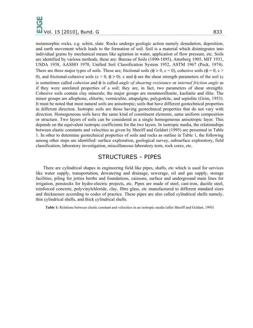
Vol. 15 [2010], Bund. G 833 metamorphic rocks, e.g. schist, slate. Rocks undergo geologic action namely denudation, deposition, and earth movement which leads to the formation of soil. Soil is a material which disintegrates into individual grains by mechanical means like agitation in water, application of flow pressure, etc. Soils are identified by various methods, these are: Bureau of Soils (1890-1895), Atterberg 1905, MIT 1931, USDA 1938, AASHO 1970, Unified Soil Classification System 1952, ASTM 1967 (Peck, 1974). There are three major types of soils. These are; frictional soils (φ > 0, c = 0), cohesive soils (φ = 0, c > 0), and frictional-cohesive soils (c > 0, φ > 0). c and φ are the shear strength parameters of the soil (c is sometimes called cohesion and φ is called angle of shearing resistance or internal friction angle as if they were unrelated properties of a soil; they are, in fact, two parameters of shear strength). Cohesive soils contain clay minerals; the major groups are montmorillonite, kaolinite and illite. The minor groups are allophone, chlorite, vermiculite, attapulgite, palygorkite, and sepiolite (Grim, 1953). It must be noted that most natural soils are anisotropic; soils that have different geotechnical properties in different direction. Isotropic soils are those having geotechnical properties that do not vary with direction. Homogeneous soils have the same kind of constituent elements, same uniform composition or structure. Two layers of soils can be considered as a single homogeneous anisotropic layer. This depends on the equivalent isotropic coefficients for the two layers. In isotropic media, the relationships between elastic constants and velocities as given by Sheriff and Geldart (1995) are presented in Table 1. In other to determine geotechnical properties of soils and rocks as outline in Table 1, the following among other steps are identified: surface exploration, geological survey, subsurface exploratory, field classification, laboratory investigation, miscellaneous laboratory tests, rock cores, etc.

STRUCTURES - PIPES

There are cylindrical shapes in engineering field like pipes, shafts, etc which is used for services like water supply, transportation, dewatering and drainage, sewerage, oil and gas supply, storage facilities, piling for jetties berths and foundations, caissons, surface and underground main lines for irrigation, penstocks for hydro-electric projects, etc. Pipes are made of steel, cast-iron, ductile steel, reinforced concrete, polyvinylchloride, clay, fibre glass, etc manufactured to different standard sizes and thicknesses according to codes of practice. These pipes are also called cylindrical shells namely, thin cylindrical shells, and thick cylindrical shells.

Table 1: Relations between elastic constant and velocities in an isotropic media (after Sheriff and Geldart, 1995)

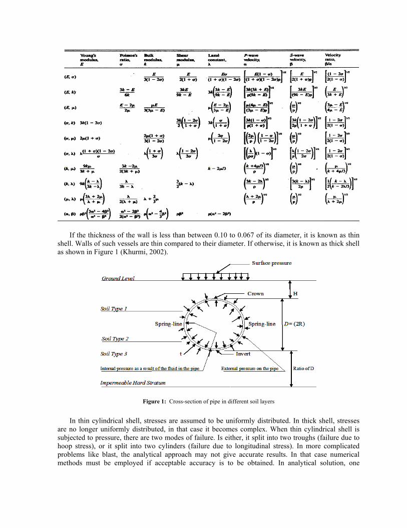
If the thickness of the wall is less than between 0.10 to 0.067 of its diameter, it is known as thin shell. Walls of such vessels are thin compared to their diameter. If otherwise, it is known as thick shell as shown in Figure 1 (Khurmi, 2002).

Figure 1: Cross-section of pipe in different soil layers

In thin cylindrical shell, stresses are assumed to be uniformly distributed. In thick shell, stresses are no longer uniformly distributed, in that case it becomes complex. When thin cylindrical shell is subjected to pressure, there are two modes of failure. Is either, it split into two troughs (failure due to hoop stress), or it split into two cylinders (failure due to longitudinal stress). In more complicated problems like blast, the analytical approach may not give accurate results. In that case numerical methods must be employed if acceptable accuracy is to be obtained. In analytical solution, one

Vol. 15 [2010], Bund. G 835 approach is the stress function concept. This was first proposed by Sir George B. Airy, later generalized for three-dimensional case by Clerk Maxwell.

2 = 0 or 4 = 0 (1)

Eq. 1 is referred to as the “biharmonic equation”. The is known as “Airy stress function”. In designing thin cylindrical shells, certain parameters must be designed for. This is to determine the required thickness of cylindrical shell for a given diameter, length and a given maximum pressure intensity. It must be remembered that lateral strain is always accompanied by linear strain. It means that lateral strain will always accompany cylindrical shell subjected to an internal pressure. Similarly there will be change in volume due to increased internal pressure. Therefore,

= = = l + 2 c (2)

Change in volume is given as,

= V ( l + 2 c) (3)

c = Circumferential strain, l = Longitudinal strain, V = Volume of the pipe, l = Length of the pipe and d = diameter of the pipe. In determining the thickness, t of cylindrical shell, efficiency of the joint should be given priority. According to Cheung and Yeo (1979) and Demeter (1996) for pipe subjected to internal pressure (Fig. 1), analytical solution for radial stress is given as,

r = (1 - ) (4)

Hoop or Tangential Stress is given as,

t = (1 + ) (5)

While the radial displacement is given as,

Ur = (6)

a is the internal radius, b is the external radius, r is radius from center to the middle of the

thickness of the pipe and P is the applied pressure. is the Poisson’s ratio and E is the Young’s modulus of the pipe material. If internal pressure and external pressure is applied in a thick-walled

cylinder with closed ends, according to Fenner (1986), the longitudinal stress set up in the cylinder wall is,

= (7)

Hoop stress, , at the internal surface is given as

- (8)

K = = (9)

Based on Lame’ theory, for thick-walled cylinders subjected to internal pressure only, neglecting

radial temperature variations, the equation of radial stress, r, is given as

r = -P (10)

Internal hoop stress is given by

hi = -P (11)

External hoop stress is given by

he = (12)

R1 is the internal radius and R2 is the external radius. These equations yield the stress distributions. The maximum values of both the radial stress and hoop stress are at the inside radius (Ross, 1996).

SOIL-PIPE INTERACTION In the analysis of soil-pipe interaction through modeling, it involves determination of soil forces

such as pressure, displacement, strain stresses, mises, etc around the pipe. Analytically, axial friction force is determined using this expression,

F = (Wp 2 DH + Wp) ( ) (13)

F = Axial friction force (N/mm), = Coefficient of friction between pipe and soil. = Density of backfill soil (kg/m3), D = Outside diameter of pipe (m), H = Depth of soil cover to top of pipe (m), Wp = Weight of pipe and content (kg/m). The soil density and friction coefficient are obtained from soil tests. Where no data are available, the following friction coefficient can be used, Silt = 0.3, Sand = 0.4, and Gravel = 0.5. Three different lateral soil forces are normally encountered in pipeline analysis; upward lateral force, downward lateral force, and sideways lateral force. There are two stages in the lateral force; elastic stage, where resistance is proportional to pipe displacement and plastic stage where resistance remains constant regardless of displacements. The lateral soil force, U, is estimated as

Vol. 15 [2010], Bund. G 837

U = (H + D) 2 tan2 (45 + ) (14)

U is the ultimate soil resistance, kg/m and other notations as previously defined. The active length of the pipe line can be determined as,

L = (15)

L is the active length (m), F is the anchor force or expansion force (kN), Q is the end resistance force (kN), f is the soil friction force (kN/m). End deflection, y is calculated as,

y = (F – Q) 2 (16)

A is the cross-sectional area of the pipe. The first is to estimate the end displacement,

y = (17)

M = (18)

Elastic constant

K = (19)

= (20)

By substitution,

Q = C - (21)

Where

C = F + (22)

y is end displacement (mm), Q is end force (kN), K is soil elastic constant, E is modulus of elasticity of pipe (kN/m2), I is moment of inertia of pipe (mm4) and M is end bending moment (kNm) (Liang-Chaun, 1978; Lester, 2008). The response of underground pipe due to blast is non-linear and can be suitably and easily solved by direct non-linear simulation (modeling).

BLAST CHARACTERISTICS The typically adopted constitutive relations of soils are elastic, elasto-plastic, or visco-plastic.

Under blast load the initial response of the constituents is the most important because it of short duration (transient). It involves some plastic deformation of soil that takes place within the vicinity of the explosion. As a

result of this one could take the ground media to be an elasto-plastic material, beyond which the soil can be considered as elastic material at distance from the explosion. Visco-elastic soils exhibit elastic behavior upon loading which is followed by slow and continuous strain increase at decreasing rate (Boh, 2007; Greg, 2008). Blast can take place above the ground surface, on the ground surface, underground or inside the structures (pipes). During explosion, surface waves and body waves are generated. Consequently there are isotropic component and deviatory component of the stress pulse. Transient stress pulse causes compression and dilation of soil and rock. This is accompanied by particle motion which is known as compression or “P”-waves while the deviatory component causes shearing stress which is known as shear or “S”-wave. On the surface of the ground, the particles adopt circular motion known as Rayleigh or “R”-wave. Compression, “P”-waves and shear, “S”-waves happens in underground explosions and they move within short range due to intervening medium which is soil or rock. On the other hand, Rayleigh, “R”-waves dominates above-ground explosions; as a result they have long range (Kameswara, 2000). Energy impulse from explosion decreases as it travels for two reasons, firstly, due to geometric effect i.e. by three dimensional dispersion of blast energy. Secondly, due to energy dissipation i.e. result of work done in plastically deforming the soil matrix.

BLAST ENERGY

The majority of explosives are formed from Carbon, Hydrogen, Nitrogen and Oxygen. The general chemical formula is Cx Hy Nw Oz. The three categories of blast are: free-air blast, air burst, and surface burst. Energy imparted to the ground by the explosion is the main source of ground shock (Ngo et al, 2007). For a sufficiently deep underground explosion, there is no blast wave. The detonation of a high explosive generates hot gases under pressure. Consequently, a layer of compressed air known as blast wave is formed. Blast wave instantaneously increases to a value of pressure above the ambient pressure. This is referred to as the side-on overpressure which decays as the shock wave expands outward from the explosion source. After a short time, the pressure behind the front may drop below the ambient pressure. TNT (trinitrotoluene) equivalent values are used to relate the performance of different explosives. This is the mass of TNT that would give the same blast performance as the mass of the explosive compound in question [34]. Conversion factors obtained from Remennikov (2003) for various explosives are; TNT (trinitrotoluene) - 1.000, RDX (Cyclonite) - 1.185, PETN - 1.282, Compound B (60% RDX 40% TNT) - 1.148, Pentolite 50/50 - 1.129, Dynamite - 1.300, and Semtex - 1.250.

Types of Blast

When a detonation occurs adjacent to and above a protective structure such that no amplification of the initial shock wave occurs between the explosive source and the protective structure, then the blast loads acting on the structure are free-air blast pressures. The air burst environment is produced by detonations which occur above the ground surface and at a distance away from the protective structure so that the initial shock wave, propagating away from the explosion, impinges on the ground surface prior to arrival at the structure. The charge detonates above the ground and the blast wave propagates with a spherical wave front. The classes of these charges falls within the aerially-delivered munitions with fuses designed to operate above the ground. A surface burst explosion will occur when the detonation is located close to or on the ground so that the initial shock is amplified at the point of detonation due to the ground reflections. The charge detonates as it comes in contact with the ground and the blast wave propagates with a hemispherical wave front. The initial wave of the explosion is reflected and reinforced by the ground surface to produce a reflected wave. Examples of these types are the terrorist vehicle bombs or military munitions fused to detonate on impact with the ground. Unlike the air burst, the reflected wave merges with the incident wave at the point of detonation to form a single wave similar to air burst but essentially hemispherical in shape. A comparison of these parameters with those of free-air explosions indicate that, at a given distance from a detonation, giving the same weight of explosive, all of the parameters of the surface burst environment are larger than those for the free-air environment (UFC, 2008). For a conservative design, surface burst is considered being the worst of the three types of blast. The charge weight of the explosive material under consideration is increased by the required

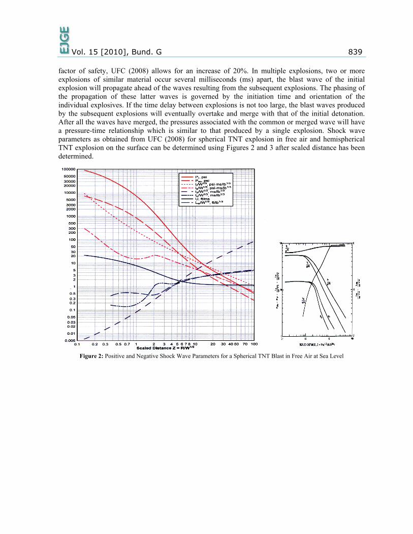
Vol. 15 [2010], Bund. G 839 factor of safety, UFC (2008) allows for an increase of 20%. In multiple explosions, two or more explosions of similar material occur several milliseconds (ms) apart, the blast wave of the initial explosion will propagate ahead of the waves resulting from the subsequent explosions. The phasing of the propagation of these latter waves is governed by the initiation time and orientation of the individual explosives. If the time delay between explosions is not too large, the blast waves produced by the subsequent explosions will eventually overtake and merge with that of the initial detonation. After all the waves have merged, the pressures associated with the common or merged wave will have a pressure-time relationship which is similar to that produced by a single explosion. Shock wave parameters as obtained from UFC (2008) for spherical TNT explosion in free air and hemispherical TNT explosion on the surface can be determined using Figures 2 and 3 after scaled distance has been determined.

Figure 2: Positive and Negative Shock Wave Parameters for a Spherical TNT Blast in Free Air at Sea Level

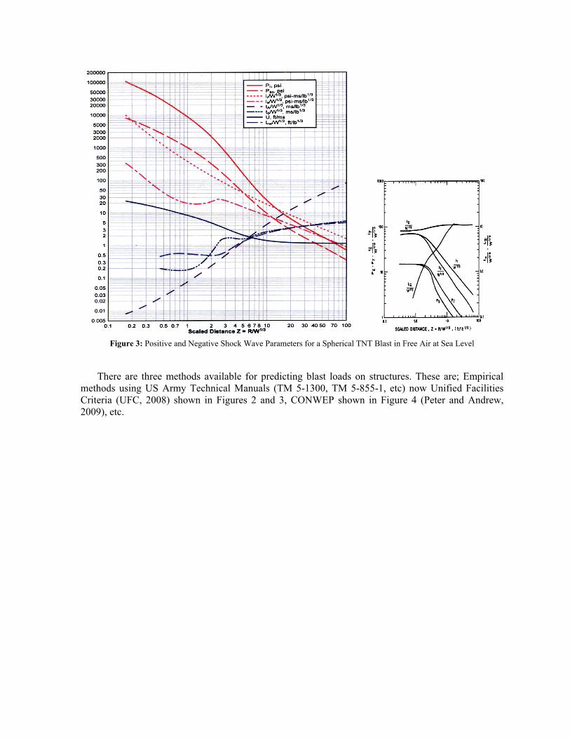
Figure 3: Positive and Negative Shock Wave Parameters for a Spherical TNT Blast in Free Air at Sea Level

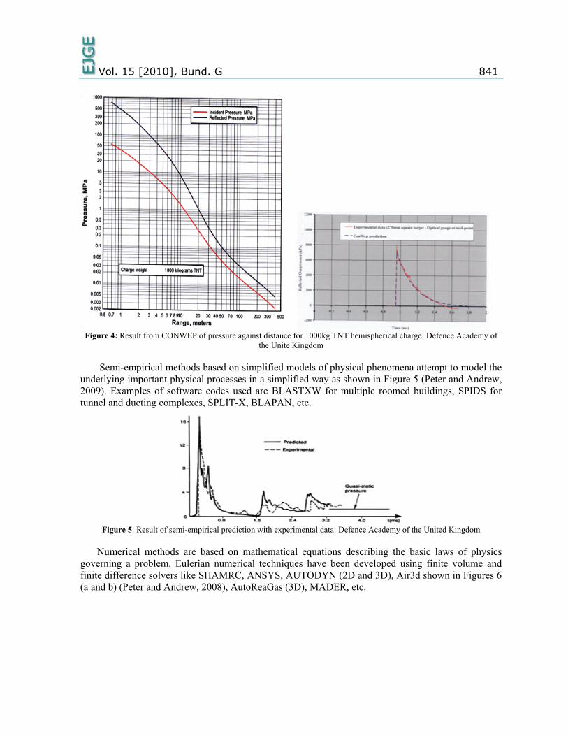
There are three methods available for predicting blast loads on structures. These are; Empirical methods using US Army Technical Manuals (TM 5-1300, TM 5-855-1, etc) now Unified Facilities Criteria (UFC, 2008) shown in Figures 2 and 3, CONWEP shown in Figure 4 (Peter and Andrew, 2009), etc.

Vol. 15 [2010], Bund. G 841

Figure 4: Result from CONWEP of pressure against distance for 1000kg TNT hemispherical charge: Defence Academy of

the Unite Kingdom

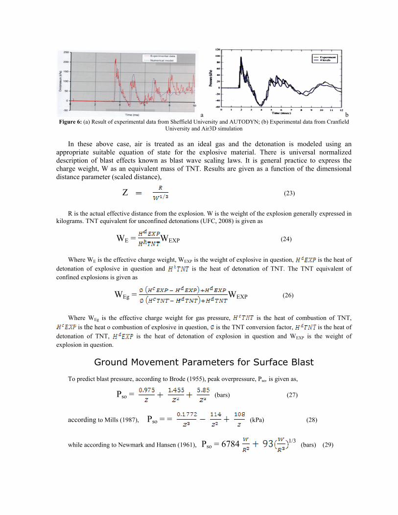
Semi-empirical methods based on simplified models of physical phenomena attempt to model the underlying important physical processes in a simplified way as shown in Figure 5 (Peter and Andrew, 2009). Examples of software codes used are BLASTXW for multiple roomed buildings, SPIDS for tunnel and ducting complexes, SPLIT-X, BLAPAN, etc.

Figure 5: Result of semi-empirical prediction with experimental data: Defence Academy of the United Kingdom

Numerical methods are based on mathematical equations describing the basic laws of physics governing a problem. Eulerian numerical techniques have been developed using finite volume and finite difference solvers like SHAMRC, ANSYS, AUTODYN (2D and 3D), Air3d shown in Figures 6 (a and b) (Peter and Andrew, 2008), AutoReaGas (3D), MADER, etc.

a b Figure 6: (a) Result of experimental data from Sheffield University and AUTODYN; (b) Experimental data from Cranfield

University and Air3D simulation

In these above case, air is treated as an ideal gas and the detonation is modeled using an appropriate suitable equation of state for the explosive material. There is universal normalized description of blast effects known as blast wave scaling laws. It is general practice to express the charge weight, W as an equivalent mass of TNT. Results are given as a function of the dimensional distance parameter (scaled distance),

Z (23)

R is the actual effective distance from the explosion. W is the weight of the explosion generally expressed in kilograms. TNT equivalent for unconfined detonations (UFC, 2008) is given as

WE = WEXP (24)

Where WE is the effective charge weight, WEXP is the weight of explosive in question, is the heat of detonation of explosive in question and is the heat of detonation of TNT. The TNT equivalent of confined explosions is given as

WEg = WEXP (26)

Where WEg is the effective charge weight for gas pressure, is the heat of combustion of TNT,

is the heat o combustion of explosive in question, is the TNT conversion factor, is the heat of detonation of TNT, is the heat of detonation of explosion in question and WEXP is the weight of explosion in question.

Ground Movement Parameters for Surface Blast

To predict blast pressure, according to Brode (1955), peak overpressure, Pso, is given as,

Pso = (bars) (27)

according to Mills (1987), Pso = = (kPa) (28)

while according to Newmark and Hansen (1961), Pso = 6784 1/3 (bars) (29)

Vol. 15 [2010], Bund. G 843

Maximum reflected pressure, Pr, when the blast encounter an obstacle is given as

Pr = 2Pso (30)

where Po is the ambient pressure. For design purposes, reflected overpressure, Pr, can be idealized by an equivalent triangular pulse of maximum peak pressure, Pr, and time duration, td (related directly to the time taken for overpressure to be dissipated), which yields the reflected positive phase impulse, ir

ir = c Pr td (c varies between 0.2 and 0.5) (31)

Air-induced ground shock results when the air-blast waves compresses the ground surface and send a stress pulse into the ground under-layers. The maximum velocity (m/s) at the ground surface expressed in terms of the peak incident overpressure (UFC, 2008) is given as

Vs = (32)

and Cp are the mass density and compression seismic wave velocity (Table 2) in the soil respectively, Vs

is the maximum vertical velocity of the ground surface.

Table 2: Compression Wave Seismic Velocities for Soils and Rocks (after UFC, 2008) Material Seismic Velocity (m/s)

Loose and dry soils Clay and wet soils Coarse and compacted soils Sand stone and cemented soils Shale and marl Limestone-chalk Metamorphic rocks Volcanic rocks Sound plutonic rocks Jointed granite Weathered rocks

182.88 - 1005.84 762 - 1920.24 914.4 - 2590.8 914.4 - 4267.2 1828.8 - 5334

2133.6 - 6400.8 3048 - 6400.8 3048 - 6858

3962.4 - 7620 243.84 - 4672 609.6 - 3048

Integrating velocity Vs with time gives maximum vertical displacement (m) of the ground surface given as,

Dv = (33)

where i is the unit positive impulse. Assuming linear velocity increase during a rise time being equal to one millisecond, and increasing acceleration by 20 percent to account for nonlinearity, vertical accelerations, Av is expressed as

Av = (34)

Where g is the gravitational constant = 9.81 m/s2. Expressing vertical motions as a function of seismic velocity of soil and shock wave,

DH = Dv tan {sin-1 (35)

VH = Vv tan {sin-1 (36)

AH = Av tan {sin-1 (37)

where U is the shock front velocity and other parameters as previously defined.

In the case of loads from direct ground shock, the peak vertical displacement in m/s at the ground surface (UFC, 2008) is given as,

Dv (rock) = 0.025 (m/s), (38)

Dv (soil) =0.17 (m/s) (39)

Where DH = 0.5 DV (40)

For dry or saturated soil, DV = DH (41)

Maximum vertical velocity for all ground media is given by VV = (42)

While VH = VV (43)

Maximum vertical acceleration, Av, in m/s2 for all ground media is given by,

Av = (44)

Duration td is related directly to the time taken for overpressure to be dissipated. Horizontal acceleration is

given by AH = 0.5 AV (45)

But for wet soil or rock media, AH = AV (46)

The arrival time tAG of shock load is a function of seismic velocity in the soil and it is expressed as

tAG = (47)

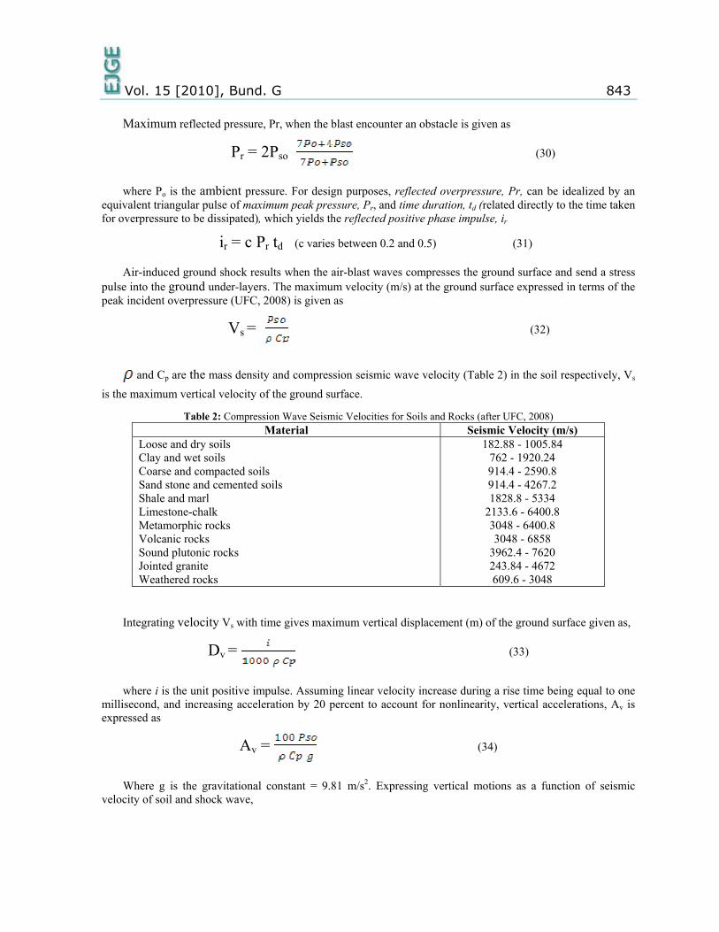
All the parameters as previously defined. For surface blast, these parameters as calculated are shown in Figure 7.

Vol. 15 [2010], Bund. G 845

Figure 7: Ground shock parameters for surface blast

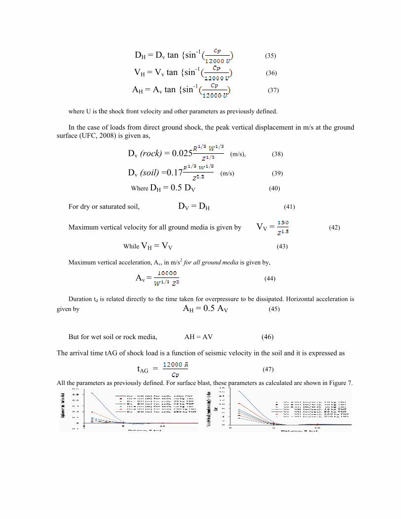
Ground Movement Parameters for Underground Blast

Ground shock parameters are equally known as the soil movement parameters which translate into loading which the soil delivers to the buried structures. These parameters are peak particle displacement which is caused by a buried explosive at a location a distance from the structure and peak particle velocity which depends on both the seismic velocity and peak particle velocity (Kameswara, 2000; Husabei, 2009). For a totally or partially buried charge located at distance R from the structure, peak particle displacement, x caused is estimated by,

x = 60 (1–n) (48)

Peak particle velocity, u, is given by

u = 48.8 Fc (-n) (49)

x is measured in meters and W is the charge mass in kg. Fc is a dimensionless coupling factor for the explosive charge which depends on explosive charge burial depth (usually taken as = 1). c is the soil seismic velocity in m/s and, n, is the dimensionless attenuation coefficient (usually taken to be = 2.75). R is the radial distance (m) measured from the center of the charge weight, W. The value of the loading wave velocity, Cp (m/s) is given by seismic velocity, c and peak particle velocity, u and is given as,

Cp (fully saturated clays) = 0.6 c + u (50)

Cp (sands) = c + u (51)

The specific impulse is then evaluated using this,

io = Cp x (52)

is the density in kg/m3 and io is measured in Ns/m2 (TM5-855-1, 1986, UFC, 2008, Zhenweng, 1997). All these parameters as calculated are shown in Figure 8.

Figure 8: Ground shock parameters for underground blast

METHODS OF ANALYSIS Many methods are available to determine the responses of underground structures most especially

pipes due to blast load. These are the analytical methods and the numerical methods. The analytic method is deterministic such as empirical phenomenological and computational fluid mechanics models which are used for blast load prediction. The problems are; it designs for elastic response or limited plastic response, and it does not allow for large deflection and unstable responses. There are several numerical methods for assessing the response of structures due to dynamic loadings. These are iteration, series methods, weighted residuals (least square methods), finite increment techniques (step by step or time integration procedure) usually referred to as finite difference, Newmark, Wilson, Newton, Houbolt, Eular, Runge-Kuta and Theta methods. Finite difference is popularly used to solve ordinary and partial differential equations, in particular, dynamic problems. Using this method, solution domain is replaced by a number of discrete points called mesh points or nodes. Solution to the problem is obtained at these points by converting the differential equation into an algebraic equation approximately satisfying the differential equation and the boundary conditions. The algebraic

Vol. 15 [2010], Bund. G 847 equations can be obtained in terms of forward, backward or central difference formulae but central difference formulae are preferred due to their higher accuracy (Kameswara, 1998).

Central Difference Method

In the central difference equations for a function U (t), in which the grid points, (i = 1, 2…n) along

the independent coordinate, t are equally spaced with step length t = h, using Taylor’s series, values of functions Ui+1 and Ui – 1 can be expressed in terms of Ui as

Ui+1 = Ui + h i + Üi + … (53)

Ui – 1 = Ui - h i + Üi + … (54)

i = |t = ti = (Ui+1 – Ui - 1) + 0(h2) (55)

Üi = |t = ti = (Ui+1 – 2Ui + Ui- 1) + 0(h2) (56)

Most of the numerical methods in dynamic analysis are based on finite difference approach. The equation of motion is given as

[m] [ ] + [c] [ ] + [k] [U] = [P] (57)

for U (t = 0) = Uo (58)

(t = 0) = o = vo (59)

Where m, c, and k are element mass, damping and stiffness matrices and t is the time. U and P are displacement and load vectors while dot indicate their time derivatives. The time duration (period) for

the numerical solution can be divided into n intervals of time t (h). It should be noted that with no damping

t

for stable and satisfactory solution or with damping

t (

is the maximum natural frequency, is the critical damping factor. Stability limit is the largest time increment that can be taken without the method generating large rapid growing

errors. The accuracy of the solution depends on the time step t = h. However, there are some conditionally stable methods where any time step can be chosen on consideration of accuracy only and need not consider stability aspect. Accordingly, the unconditionally stable methods allow a much larger step for any given accuracy. Replacing Eq.57 by Eq. 55 and 56, we have

m {{U (i+1) – 2 i + U(i-1)} / } + c{{U(i+1) – U(i-1)} / }} kUi = P (60)

where Ui = U(ti) and Ui+1 can be written as

U(i+1) = [ Ui + U(i-1) + Pi] (61)

This is the recurrence formula which gives the value of Ui+1 in terms of Ui, Ui – 1 and Pi. Repeated use of the recurrence equation gives the response of U of the system in the entire domain of interest. This is also called an explicit integration method since Ui+1 is obtained by using the dynamic equilibrium of the system at ti as given in Eq. 60. The solution can not start by itself, because to obtain Ui (i = 0) from Eq 61, there is need to get the values Uo and U-1. Uo is given by the initial condition

in Eq. 58, U-1 has to be generated using the other initial conditions o given by Eq. 60 and the governing equation of motion (Eq. 57) is given by

Üo = (m)-1 (Po – c o – kUo) (62)

From the difference equations (Eqs. 55 and 56), we obtained

U -1 = Uo - h o + Üo (63)

where Üo is known from the given initial conditions as expressed by Eq. 62, i is increment number of an exp[licit dynamic step and dots indicate their time derivatives. This could be solved using Abaqus dynamic explicit which uses explicit central difference operator that satisfies the dynamic equilibrium equations at the beginning of the increment, t, the acceleration calculated at time, t are

used to advance the velocity solution to time, t + and displacement solution to time, t + t. Dynamic In direct-integration dynamics of time integration in the Abaqus Explicit, the equations of motion (Eqs. 57, 60, 61, 62 and 63) of the system is integrated through out time. This makes it unnecessary for the formation and inversion of the global mass and stiffness matrices [M], [K]. It also simplifies the treatment of contact and requires no iteration. This means that each increment is relatively inexpensive compared to the increments in an implicit integration scheme. It performs a large number of small increments efficiently. Explicit are used for the analysis of large models with relative short dynamic response times and extremely discontinuous events or processes (Abaqus Manual, 2009; Olarewaju et al, 2010). Other numerical tools like ANSYS, AUTODYN 2D and 3D, FLAC 2000, etc could suitably be used.

Technical Design Manuals for Blast-Resistant Design Structures to Resist the Effects of Accidental Explosions, TM 5-1300 (U.S. Departments of the Army,

Navy,, and Air Force, 1990), A Manual for Prediction of Blast and Fragment Loadings on Structures, DOE/TIC-11268 (U.S.

Department of Energy, 1992), Protective Construction Design Manual, ESL-TR-87-57 (Air Force Engineering and Services Center,

1989), Fundamentals of Protective Design for Conventional Weapons, TM 5-855-1 (U.S. Department of the

Army, 1986), The Design and Analysis of Hardened Structures to Conventional Weapons Effects (DAHS CWE,

1998), Structural Design for Physical Security – State of the Practice Report (ASCE, 1995),

Vol. 15 [2010], Bund. G 849

Principles and Practices for Design of Hardened Structures, Number AFSWC-TDR-62-138, (Air Force Design Manual, Technical Documentary Report, 1962),

Unified Facilities Criteria (2008), “Structures to Resist the Effects of Accidental Explosions”, UFC 3-340-02, Department of Defense, US Army Corps of Engineers, Naval Facilities Engineering Command, Air Force Civil Engineer Support Agency, United States of America (This manual supersede TM5-1300 (1990)), etc.

MODELING Methods of structural analysis and design are broadly divided into three, firstly, theoretical

methods which carrying out analysis and the use of design codes, secondly, by testing full size structure using experimental method and thirdly by the use of models (simulations) where the first two failed like structures of complicated shapes. Structural problems demanding model studies (simulations) are to:

predict the behavior of complicated structures with irregular boundaries, design structures with complex supports and loading conditions, get direct aids in design i.e. it offer short cut to design, check the design of very important and expansive structures such as large span bridges, prestige

buildings, atomic reactors, cooling towers, shell structures, check the validity of analytical procedures, investigate failure of structures caused by wrong assumptions, crude approximations of structural

behavior, etc, and make qualitative demonstrations of structural behavior vis-à-vis simple structural action, deformed

shapes, points of contraflexure, modes of buckling and collapse, reciprocal theorem, principle of superposition, etc (Ganesan, T. P, 2000).

Finite Element Modeling

In finite element model, real continuous structure is idealized into assemblage of discrete elements. Force-displacement relations and stress distributions are determined or assumed. The complete solution is obtained for the entire structure by combining the individual elements into an idealized structure. Conditions of equilibrium and compatibility are satisfied at the junctions of these elements. One-dimensional, two-dimensional and three-dimensional finite elements such as triangular, rectangular, hexahedron, tet, wedge, etc can be used. Advantages of this method are; much greater flexibility both in fitting boundary shapes, in arranging internal distributions of nodal points to suit particular problems, and lastly it provides a great deal of information concerning the variations of unknowns at points within the region of interest. The disadvantage is the expertise required and substantially increased storage requirement for equation coefficients. In modeling, damping may be specified as part of a material definition that is assigned to a model. Abaqus has elements such as dashpots, springs and connectors that serve as dampers, all with viscous and structural damping factors. It equally allows the specification of global damping factors for both viscous (Rayleigh damping) and structural damping (imaginary stiffness matrix). One can use choose to model the viscous damping matrix by using material damping properties and/or damping elements (such as dashpot or mass element) (Abaqus Manual, 2009). Contrary to our usual engineering intuition, introducing damping to the solution reduces the stable time increment. Raleigh damping is meant to reflect physical damping in the actual material. A small amount of numerical damping could be introduced in the form of bulk viscosity to control high frequency oscillations. The boundary conditions of the finite element model for displacements could be fixed at the base and roller on all the

four sides. This is to simulate infinity of the soil medium despite the short duration of the blast problem, and to allow the energy to dissipate away without reflecting back into the soil and buried pipes (Olarewaju et al, 2010). Apart from Abaqus numerical code, FLAC, ANSYS, AUTODYN 2D, AUTODYN 3D, etc could be used to study the response of underground structures (pipes) by modeling while SAP program could be used to study linear response.

CONCLUSION This paper has highlighted the basic steps in the study of response of underground pipes due to

blast loads. Blast characteristics were also critically examined. Analytical and numerical methods of analysis were considered for the response of underground pipes due to static and dynamic load. It must be noted that soil exists as a semi-infinite half space. Numerical methods to be employed must incorporate the notion of infinity in the formation. Integral equation method and boundary element method can handle infinite domain naturally. Finite difference and finite element methods are domain descritization methods. They can not be applied to semi-infinite domain directly. A way out of handling such infinite domains is by considering a finite domain for descritization with approximate boundary conditions. Exact solutions to general partial differential equations are difficult to obtain due to irregular and geometrically complicated domains. There is difficulty in applying finite difference method and variational methods, this difficulties lies in considering approximate functions of the dependent variable. These functions need to satisfy the geometric boundary conditions on irregular domains which are suitably considered in numerical tool like ABAQUS software package. Other software packages like ANSYS, AUTODYN 2D and 3D, PLAXI, FLAC 2000, etc could suitably be used for linear and non-linear response.

ACKNOWLEDGEMENT The project is funded by Ministry of Science, Technology and Innovation, MOSTI, Malaysia

under e-Science Grant no. 03-01-10-SF0042.

REFERENCES 1. Abaqus Inc, (2009) ABAQUS User’s Manuals - Documentation, Version 6.8-EF, D’S

Simulia, Providence, Rhode Island, USA,

2. Boh, J. W., Louca, L. A. and Choo, Y. S., (2007) “Finite Element Analysis of Blast Resistance Structures in the Oil and Gas Industry”, Singapore and UK, ABAQUS User’s Conference, pp 1-15,

3. Butcher, K., Crown, L., and Gentry, E. J., (2006) “The International System of Units (SI) – Conversion Factors for General Use”, Weights and Measures Division, Technology Services, NIST Special Publication 1038, US

4. Chen, W. F. (1995) “The Civil Engineering Handbook”, CRC Press, London,

5. Cheung, Y. K. and Yeo, M. F. (1979) “A Practical Introduction to Finite Element Analysis”, Fearon Pitman Publishers Inc., San Francisco, pp 40-72

6. Converse, F. J. (1953) “Compaction of sand at resonant frequency”, Symposium on Dynamic Testing of Soils, ASTM Special Technical Publication No. 156, pp 124-137,

7. ConWep, (1991) “ Conventional weapons effects program, Prepared” by DW Hyde, ERDC Vicksburg MS,

Vol. 15 [2010], Bund. G 851

8. Demeter, G. F., (1996) “Advanced Mechanics of Structures”, Marcel Dekker Inc., New York, pp 404-420,

9. Fenner, R. T. (1986) “Engineering Elasticity: Application of Numerical and Analytical Techniques”, Ellis Harwood Ltd., England, pp 166-176

10. Frans Alferink, (2001) “Soil-Pipe Interaction: A next step in understanding and suggestions for improvements for design methods”, Waving M & T, The Netherlands, Plastic Pipes XI, Munich, 3rd-6th September,

11. Ganesan, T. P. (2000) “Model of Structures”, First Edition, University Press Ltd., India,

12. Greg B. C. (2008) “Modeling Blast Loading on Reinforced Concrete Structures with Zapotec”, Sandia National Laboratories, Albuquerque, ABAQUS User’s Conference,

13. George, P. K., George, D. B. and Charis, J. G. (2007) “Analytical calculation of blast-induced strains to buried pipelines”, International Journal of Impact Engineering, Vol. 34, pp 1683-1704,

14. Grim, R. E. (1953) “Clay Mineralogy”, McGraw-Hill, New York,

15. Husabei Liu, (2009) “Dynamic Analysis of Subways Structures under Blast Loading”, University Transportation Research Center, New York, USA,

16. James A. Marusek, (2008) “Personal Shelters”, Abaqus User’s Conference, US Department of the Navy,

17. Johnson, D. (1986) “Advanced Structural Mechanics, An Introduction to Continuum Mechanics and Structural Dynamics”, Collins, London,

18. Kameswara Rao, N. S. V., (2000) “Dynamic Soil Tests and Applications”, First Edition, Wheeler Publishing Co. Ltd., New Delhi, India,

19. Kameswara Rao, N. S. V., (1998) “Vibration Analysis and Foundation Dynamics”, Wheeler Publishing Co. Ltd., New Delhi, India,

20. Khurmi, R. S. (2002) “Strength of Materials”, Chand S. and Company Ltd., New Delhi,

21. Lamb, H. (1904) “On the propagation of tremors over the surface of an elastic solid”, Philosophical Transactions of the Royal Society, Vol. 203: pp 1-42,

22. Lester, H. G. (2008) Chapter 4: “The Pipe/Soil Structure – Actions and Interactions”,

23. Liang-Chaun Peng, (1978) “Soil-pipe interaction - Stress analysis methods for underground pipelines”, AAATechnology and Specialties Co., Inc., Houston, Pipeline Industry, May, pp 67-76,

24. Naury, K. B., Richard, A. G., Greg, E. F., Colin, J. H. and Nigel, J. F. (2008) “Analysis of Blast Loads on Building”, Century Dynamics Incorporated Limited, Oakland, CA,

25. Newcomb, W. K. (1951) “Principles of Foundation Design for Engines and Compressors”, Trans of the ASME, Vol. 73, pp 307 318,

26. Newmark, N. M. and Haltiwanger, J. D. (1962) “Air Force Design Manual, Principles and Practices for Design of Hardened Structures”, Technical Documentary Report Number AFSWC-TDR-62-138,

27. Newmark, N. M. and Hansen, R. J. (1961) “Design of blast resistant structures”, Shock and Vibration Handbook, Vol. 3, Eds. Harris and Crede., McGraw-Hill, New York, USA,

28. Ngo, T. J., Mendis, J., Gupta, A. and Ramsay, J. (2007) “Blast Loading and Blast Effects on Structures – An Overview”, University of Melbourne, Australia, EJSE International Special Issue: Loading on Structures, pp 76-91,

29. Olarewaju, A. J., Kameswara Rao N.S.V and Mannan, M.A., (2010), “Response of Underground Pipes due to Blast Load”, Proceedings of the 3rd International Earthquake Symposium, Bangladesh, (3-IESB), Bangladesh University of Engineering Technology, Dhaka, March 4th-6th, pp 165-172,

30. Peck, R. B., Hanson, W. E., and Thornburn, T. H. (1974) “Foundation Engineering”, Second Edition, Wiley, New York,

31. Peter, D. S. and Andrew, T. (2009) “Blast Load Assessment by Simplified and Advanced Methods”, Defence College of Management and Technology, Defence Academy of the United Kingdom, Cranfield University, UK,

32. Ravu Venugopala Rao, (1995) “Time Domain Analysis of Three Dimensional Soil-Structure Interaction Problems”, Ph.D thesis, Department of Civil Engineering, Indian Institute of Technology, Kanpur, India,

33. Remennikov, A. M. (2003) “A Review of Methods for Predicting Bomb Blast Effects on Buildings”, University of Wollongong, Journal of Battlefield Technology, Vol. 6, No. 3, pp 5-10,

34. Robert, W. D. (2002) “Geotechnical Earthquake Engineering Handbook”, McGraw-Hill, New York,

35. Ronanki, S. S. (1997) “Response Analysis of Buried Circular Pipes under 3-Dimensional Seismic Loading”, M.Tech thesis, Civil Engineering Department, Indian Institute of Technology, Kanpur, India,

36. Ross, C. T. F. (1996) “Finite Element Techniques in Structural Mechanics”, First Edition, Albion Engineering Science Series, Chichester, pp 1-95,

37. Ross, C. T. F. (1996) “Mechanics of Solids”, Prentice Hall, London. Pp 233-253, 308-338,

38. Sherif R. E. and Geldart L. P. (1995), Exploration Seismology, Second edition, Cambridge University Press, London, Dec. Pp 69,

39. Unified Facilities Criteria, (2008), “Structures to Resist the Effects of Accidental Explosions”, UFC 3-340-02, Department of Defense, US Army Corps of Engineers, Naval Facilities Engineering Command, Air Force Civil Engineer Support Agency, United States of America,

40. US Army Engineers Waterways Experimental Stations, (1986) “Fundamental of Protection Design for Conventional Weapons”, TM 5-855-1, Vicksburg,

41. Zhenweng Yang, (1997) “Finite element simulation of response of buried shelters to blast loadings”, National University of Singapore, Republic of Singapore, International Journal of Finite Element in Analysis and Design, Vol. 24, Elsevier, pp 113-132.

© 2010 ejge