i

RESPONSE OF EXTENDED EULER-BERNOULLI BEAM UNDER

IMPULSE LOAD USING WAVELET SPECTRAL FINITE ELEMENT

METHOD

A THESIS

submitted by

MALLIKARJUN B

for the award of the degree

of

MASTER OF TECHNOLOGY

STRUCTURAL ENGINEERING DIVISION

DEPARTMENT OF CIVIL ENGINEERING

NATIONAL INSTITUTE OF TECHNOLOGY, ROURKELA 769008

May 2012

ii

CERTIFICATE

This is to certify that the thesis entitled “RESPONSE OF EXTENDED EULER-

BERNOULLI BEAM UNDER IMPULSE LOAD USING WAVELET SPECTRAL

FINITE ELEMENT METHOD” submitted by Mallikarjun B in partial fulfillment of the

requirement for the award of Master of Technology degree in Civil Engineering with

specialization in Structural Engineering to the National Institute of Technology, Rourkela is an

authentic record of research work carried out by him under my supervision. The contents of this

thesis, in full or in parts, have not been submitted to any other Institute or University for the

award of any degree or diploma.

Project Guide

Rourkela-769 008 Dr. Manoranjan Barik

Date: Associate Professor

Department of Civil Engineering

iii

ACKNOWLEDGEMENTS

First and foremost, praise and thanks goes to my God for the blessing that has been bestowed

upon me in all my endeavors.

I am deeply indebted to Dr. Manoranjan Barik, Associate Professor, my advisor and guide, for

the motivation, guidance, tutelage and patience throughout the research work. I appreciate his

broad range of expertise and attention to detail, as well as the constant encouragement he has

given me over the years. There is no need to mention that a big part of this thesis is the result of

joint work with him, without which the completion of the work would have been impossible.

I extend my sincere thanks to the Head of the Civil Engg Department Prof. N. Roy, for his

advice and unyielding support over the year.

The personal communication and discussion with Dr. Mira Mitra of Indian Institute of

Technology, Bombay is of immense help. Her valuable suggestions and timely co-operation

during the project work is highly acknowledged. The author extends his heartfelt thanks to her.

I would like to take this opportunity to thank my Parents and my sister for their unconditional

love, moral support, and encouragement for the timely completion of this project.

I am grateful for friendly atmosphere of the Structural Engineering Division and all kind and

helpful professors that I have met during my course.

I express my most sincere admiration to my friends, (in no particular order) Bijily B., Suji P,

Venkateshwara Reddy and to all my classmates for their cheering up ability which made this

project work smooth.

iv

So many people have contributed to my thesis, my education, and it is with great pleasure to take

the opportunity to thank them. I apologize, if I have forgotten anyone.

Mallikarjun B

Roll No: 210ce2022

M.Tech (Structures)

v

PREFACE

Transform methods are some of those methods which are able to solve certain difficult ordinary

and partial differential equation. The most commonly used transform for these solutions are

Laplace and Fourier transforms. Wavelet transforms are new entrants in to this area, although

they are quite popular with electrical and communication engineers in characterizing and

synthesizing the time signals. The utility of wavelet transforms is shown in structural engineering

by addressing problems involving solutions of ordinary and partial differential equations

encountered in dynamical related problems.

Dynamical problems in structural engineering fall under two categories, one involving low

frequencies, which is called structural dynamics problems, and the other involving very high

frequencies, which is called the wave propagation problems. The most problems in structural

engineering fall under the former category, wherein the response of the entire structural system is

characterized using only the first few vibrational modes. The wave propagation is a multi-modal

phenomenon involving vibrational modes of very high frequencies. Conventional analysis tools

such as finite element cannot handle these problems due to modeling limitations and extensive

computational cost. The only alternative to such problems is the method based on transforms.

Spectral finite element (SFE) method is one such transform method, which can be a viable

alternative to solving problems involving high frequency excitations. SFE based on Fourier

transform is quite well known and established. However, it has severe limitations in handling

finite structures and specifying non-zero boundary/initial conditions, and thus its utility in

solving real world problems involving high frequency excitation is limited.

vi

The aim of the present work is to show that the wavelet transform is very useful in solving

ordinary differential equations by modeling the structure as a discrete system involving structural

dynamic problems and it is to use wavelet transform to solve those problems involving partial

differential equations. In this work, the response of an cantilever Extended Euler-Bernoulli

aluminum beam under impulse load applied axial and transverse at the free end is shown. The

response is being obtained by coding programs in MATLAB.

vii

Contents PREFACE ...................................................................................................................................v

List of Figures ........................................................................................................................... ix

List of Tables ..............................................................................................................................x

List of symbols.......................................................................................................................... xi

1 Introduction ............................................................................................................................1

1.1 Overview ...........................................................................................................................2

1.1.1 Solution methods for structural dynamics problems ...................................................2

1.1.2 Solution Methods for Wave Propagation Problems ....................................................3

1.2 Numerical methods for solving PDEs...............................................................................6

1.2.1 Finite difference method ............................................................................................7

1.2.2 Spectral method .........................................................................................................7

1.2.3 Wavelet Galerkin method ..........................................................................................7

1.3 Fourier analysis................................................................................................................8

1.3.1 Continuous Fourier Transforms .................................................................................9

1.3.2 Discrete Fourier Transform...................................................................................... 10

1.3.3 Windowed Fourier transforms ................................................................................. 13

1.3.4 Fast Fourier Transforms .......................................................................................... 13

2 Literature Review ................................................................................................................. 14

3 Wavelet Analysis ................................................................................................................. 25

3.1 What is wavelet analysis? .............................................................................................. 26

3.2 Definitions of terms used ............................................................................................... 26

3.2.1 Orthogonal/Non-orthogonal ..................................................................................... 26

3.2.2 Symmetry ................................................................................................................ 27

3.2.3 Vanishing Moments................................................................................................. 27

3.2.4 Compact Support ..................................................................................................... 27

3.2.5 Scaling .................................................................................................................... 28

3.2.6 Wavelet and Scaling Functions .............................................................. 28

3.3 Wavelet Transforms: ...................................................................................................... 29

3.3.1 Daubechies Wavelet (db) ......................................................................................... 29

3.3.2 Multi-Resolution Analysis (MRA) with Wavelets.................................................... 30

viii

3.3.3 Daubechies compactly supported wavelets .............................................................. 33

3.3.4 Construction of Daubechies Compactly Supported Wavelets ................................... 33

3.4 Moment of Scaling Functions ( ) ............................................................................... 41

4 Spectral Analysis .................................................................................................................. 43

4.1 Spectrum and Dispersion relations ................................................................................. 44

4.2 Computations of wavenumbers and wave amplitudes ..................................................... 51

4.2.1 Singular value decomposition (SVD) ....................................................................... 54

4.3 Spectral Finite Element Method (SFEM) ....................................................................... 55

5 Wavelet Spectral Finite Element........................................................................................... 58

5.1 Reduction of rod wave equation to ordinary differential equations ................................. 60

5.2 Boundary conditions ...................................................................................................... 65

5.2.1 Non-perodic boundary conditions ............................................................................ 65

5.3 Decoupling using eigenvalue analysis ............................................................................ 68

5.4 Reduction of beam wave equation to ordinary differential equations .............................. 70

5.5 Boundary conditions ...................................................................................................... 74

5.5.1 Non-perodic boundary conditions ............................................................................ 74

5.6 Decoupling using eigenvalue analysis ............................................................................ 77

6 Wavelet Spectral Finite Element Formulation ....................................................................... 79

6.1 Spectral element formulation for Extended Eular-Bernoulli beam .................................. 80

7 RESULTS & DISCUSSION ................................................................................................ 84

7.1 Results of spectral finite element formulation .................................................................... 86

7.2 Response of Extended Euler-Bernoulli aluminum beam under axial impulse load .......... 88

7.3 Response of Extended Euler-Bernoulli aluminum beam under transverse impulse load .. 93

8 Conclusion ........................................................................................................................... 95

References ................................................................................................................................ 97

ix

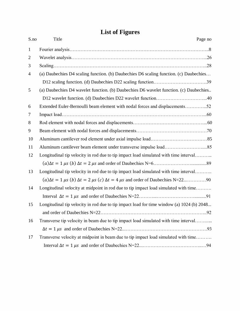
List of Figures S.no Title Page no

1 Fourier analysis……………………………………………………………………………..8

2 Wavelet analysis…………………………………………………………………………...26

3 Scaling……………………………………………………………………………………..28

4 (a) Daubechies D4 scaling function. (b) Daubechies D6 scaling function. (c) Daubechies…

D12 scaling function. (d) Daubechies D22 scaling function…………………………….39

5 (a) Daubechies D4 wavelet function. (b) Daubechies D6 wavelet function. (c) Daubechies..

D12 wavelet function. (d) Daubechies D22 wavelet function…………………………...40

6 Extended Euler-Bernoulli beam element with nodal forces and displacements…………..52

7 Impact load………………………………………………………………………………...60

8 Rod element with nodal forces and displacements………………………………………...60

9 Beam element with nodal forces and displacements………………………………………70

10 Aluminum cantilever rod element under axial impulse load………………………………85

11 Aluminum cantilever beam element under transverse impulse load……………………....85

12 Longitudinal tip velocity in rod due to tip impact load simulated with time interval………..

and order of Daubechies N=6…………………….............89

13 Longitudinal tip velocity in rod due to tip impact load simulated with time interval………..

and order of Daubechies N=22...…………90

14 Longitudinal velocity at midpoint in rod due to tip impact load simulated with time……….

Interval and order of Daubechies N=22………...……………………..........91

15 Longitudinal tip velocity in rod due to tip impact load for time window (a) 1024 (b) 2048...

and order of Daubechies N=22…………………………………………………………..92

16 Transverse tip velocity in beam due to tip impact load simulated with time interval……......

and order of Daubechies N=22...…………………………………………….93

17 Transverse velocity at midpoint in beam due to tip impact load simulated with time……….

Interval and order of Daubechies N=22...………………………………..…94

x

List of Tables Table no Title Page no

1 Filter coefficients…………………………………………………………...38

2 Moment of scaling functions……………………………………………….42

3 Connection coefficients………………………………………………….…64

4 Wave numbers……………………………………………………………...86

xi

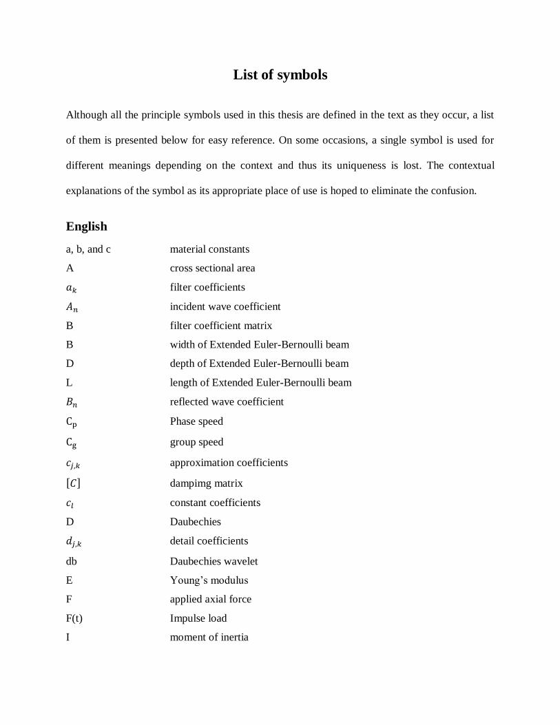
List of symbols

Although all the principle symbols used in this thesis are defined in the text as they occur, a list

of them is presented below for easy reference. On some occasions, a single symbol is used for

different meanings depending on the context and thus its uniqueness is lost. The contextual

explanations of the symbol as its appropriate place of use is hoped to eliminate the confusion.

English

a, b, and c material constants

A cross sectional area

filter coefficients

incident wave coefficient

B filter coefficient matrix

B width of Extended Euler-Bernoulli beam

D depth of Extended Euler-Bernoulli beam

L length of Extended Euler-Bernoulli beam

reflected wave coefficient

Phase speed

group speed

approximation coefficients

[ ] dampimg matrix

constant coefficients

D Daubechies

detail coefficients

db Daubechies wavelet

E Young‟s modulus

F applied axial force

F(t) Impulse load

I moment of inertia

xii

I Complex √

J dilation indices

k wave number

[k] stiffness matrix

[ ] elemental dynamic stiffness matrix

M vanishing moments

[ ] global mass

N Order of Daubechies

n Sampling points

p polynomial of order

nodal force

nodal shear force

nodal moment

[R] amplitude ratio matrix

T total period

t time

axial diaplacement

{ } acceleration

{ } velocity

{ } displacement

{ } nodal displacement vector

spatial coordinates

xs arbitrary points

tranverse displacment

xiii

Greek

circular frequency

time interval between two sampling points.

wavelet function or mother wavelet

scaling function or father wavelet

first derivative of scaling function

second derivative of scaling function

first order connection coefficients

second order connection coefficients

first order connection coefficient matrices.

second order connection coefficient matrices.

eigenvector matrix of

diagonal matrix containing corresponding eigenvalues

diagonal matrix with diagonal terms

[ ] diagonal matrix with diagonal terms

Moment of scaling functions

frequency of transition

cut off frequency

dampimg ratio

density of material

1 | P a g e

CHAPTER ~ 1

1 Introduction

2 | P a g e

1.1 Overview

Wavelets are effectively used for signal processing and solution of differential equations.

Wavelet transform is implemented to solve and analyze problems associated with engineering

mechanics. The use of wavelets in mechanics can be viewed from different perspectives, such as

the analysis of mechanical responses for extraction of model parameters, de-noising, damage

measures etc. the solution of the differential equations governing the mechanical system; the

solution of structural dynamics and wave propagation problems using wavelet transform

methods.

Structural dynamics deal with lower frequencies in the magnitude of a few hundred Hertz, or

only the first few modes of vibrations and involve the study of steady state response. On the

other hand, wave propagation results from high frequency excitations, in the order of Kilohertz

and involves the study of transient response.

1.1.1 Solution methods for structural dynamics problems

The solution of structural dynamics problems can either be the determination of system

parameters, mostly, natural frequencies and mode shapes, or simulations of the response of the

system to external excitations such as initial displacements, external load, support motion etc.

For a discrete system, i.e. a multi-degree of freedom (MDOF) system, the governing equations

(ODEs) are coupled in general.

Apart from wavelet analysis of structural dynamics, this mainly concentrates on wavelet-based

spectral analysis of wave propagation. A numerical scheme called wavelet-based spectral finite

element method is implemented for modeling of an Extended Euler-Bernoulli beam. This

technique helps the computational efficiency of spectral analysis while possessing several

3 | P a g e

advantages over Fourier transform-based spectral analysis particularly for capturing near field

phenomena.

1.1.2 Solution Methods for Wave Propagation Problems

Wave propagation is a transient dynamic phenomenon resulting from short duration loading.

Such transient loadings have high frequency content. The main difference between the structural

dynamics and wave propagation in structures arises due to high frequency excitations. Structures

very often experience such loadings in forms of impact and blast loadings like gust, bird hit, tool

drops etc. Apart from understanding the behavior of structures under such loadings, wave

propagation analysis is also important to gain knowledge about their high frequency

characteristics which have several applications. The applications include structural health

monitoring using diagnostic waves and control of wave transmission for reduction of noise and

vibration.

Though finite element (FE) method is versatile and widely used to model complex structures for

structural dynamics problem, it is highly unsuited for wave propagation analysis. Higher

frequency content of the loading in wave propagation problems requires very fine mesh with the

element size comparable to the wave lengths, which are very small at higher frequencies. This

results in large system size and huge computational cost. In addition to the fine mesh, to obtain

system response, the mode superposition method or time integration schemes have to be

implemented after FE modeling. Mode superposition method cannot be applied for wave

propagation analysis. This is because for such problems the model parameters have to be

extracted over a wide range of frequency. This has to be done through eigen value analysis

which is computationally very expensive. Alternatively there are several time integration

schemes used for solution of dynamic problems. These schemes can be used for simulation of

4 | P a g e

wave response. In these methods, analysis is performed over a small time step, which is a

fraction of the total time for which the response histories are required. For some time integrations

schemes, however, a constraint is placed on the time step, and this coupled with large system

sizes makes the FE solution of wave propagation problems computationally prohibitive. The

alternative numerical techniques are adopted for these problems and several such techniques are

Boundary Element Method (BEM) [7, 41], discontinuous Galerkin method [61, 24], Mesh less

Local Petrov-Galerkin (MLPG) method [8], wave finite element method [65] etc.

Among these techniques, many methods are based on integral transform [18] which include

Laplace transform, Fourier transform, and most recently wavelet transform. In these methods,

first the governing equations are transformed to the frequency domain using the forward

transform in time. Such transformation reduces the governing PDEs by one dimension to

differential equations with only spatial variations. The solution of these transformed equations is

much easier than the original PDEs and often has analytical solution. These solutions in

transformed frequency domain contain information of several frequency dependent wave

properties essential for the analysis. The time domain solution is then obtained through inverse

transform. The use of Laplace transform for solution of wave equation has been limited because

of the difficulty in performing the inverse transform. On the other hand, the application of

continuous Fourier transform (CFT) for such purpose has been reported [63], but even here, the

inverse transform required is difficult to obtain and, these methods are suited only for far-field

behavior like seismological studies.

In structural wave propagation, the structures are finite, and hence these schemes are not

adequate since due to inherent problems in obtaining the transform, it cannot provide information

about the reflection of waves on interaction between different boundaries and discontinuities.

5 | P a g e

The forward and inverse discrete Fourier transform (DFT), however can be numerically

implemented. Fast Fourier transform (FFT) is the easy and fast algorithm for DFT. Spectral finite

element (SFE) is one such method on Fourier transform and initially proposed by Narayanan and

Beskos [59] and popularized by Doyle and his co-researchers [16]. In SFE, the differential

equations are reduced to ODEs using Fourier transform in time. The solution gives the

transformed displacements, which are converted to the displacements in time domain through

inverse transform. The SFE technique like the other integral transform-based methods is

effective in handling inverse problems like force identification and system identification.

From the mathematical explanation of wavelets, the wavelets are potential for spectral finite

element formulation. There are several wavelets like Daubechies orthogonal wavelets, bi-

orthogonal spline (B-spline) wavelets, interpolation wavelets, which have compactly supported

bases with local supports and orthogonal properties. Thus they can be used to solve partial

differential wave equations through integral transform because of the following advantages.

Firstly, wavelet allows finite domain analysis and imposition of initial or boundary conditions

which are possible due to the local support of these basis functions. Secondly, these bases are

bounded both in time and frequency domains. However, the resolution in frequency domain may

be reduced when compared to Fourier transform-based SFE and this is the trade-off to obtain

better resolution in time domain analysis.

Wavelets have several encouraging properties for their use in numerical solution of partial

differential equations (PDEs). The researchers [1, 20, 29, 17] have provided a review of wavelet

techniques for solution of PDEs. The orthogonal, compactly supported wavelet basis of

Daubechies [13, 15], exactly approximates polynomial of increasingly higher order. These

wavelet bases can provide accurate and stable representation of differential operations even in

6 | P a g e

region of strong gradients or oscillations. In addition, it has the advantage of multi resolution

analysis over the traditional methods. The main drawback of Fourier based spectral approach is

that it cannot handle waveguide of short lengths. This is because, short lengths forces multiple

reflections at smaller time scales. Since Fourier transforms are associated with a finite time

window, shorter length of waveguide do not allow the response to die down within the chosen

time window, irrespective of the type of damping used in modeling. These forces the response to

wrap around, that is the remaining part of the response beyond the chosen time window, will

start appearing first. This totally distorts the response. It is in such cases compactly supported

wavelets, which have localized basis functions, can be efficiently used for waveguide of short

lengths. Different wavelet based modeling techniques for simulations of wave propagation have

been presented [25].

In the present work an approach similarly to SFEM is followed. Daubechies scaling functions are

used for approximation in time and this reduces the PDE to ODEs in spatial dimension. These

ODEs formed are coupled unlike those in FFT based SFEM (FSFEM). The system of coupled

ODEs is decoupled performing an eigenvalue analysis, which decreases the computational cost

considerably. The eigen analysis involved is time consuming, but this can be computed and

stored as it is not related to the particular problem. The decoupled ODEs are then solved

similarly as in SFEM and a wavelet based spectral element (WSFE) is formulated.

1.2 Numerical methods for solving PDEs

A brief introduction about some numerical methods to solve the PDEs

7 | P a g e

1.2.1 Finite difference method

Finite Difference Method (FDM) is most commonly used method to solve Ordinary Differential

Equations (ODEs) and PDEs in a bounded domain. The basic idea of finite difference methods is

simple: derivatives in differential equations are written in terms of discrete quantities of

dependent and independent variables, resulting in simultaneous algebraic equations with all

unknowns prescribed at discrete nodal points for the entire domain. For example, the order of

convergence in second order FDM is (N−2) where N is number of nodal points. In brief about

FDM, the different unknowns are defined by their values on discrete (finite) grid and differential

operators are replaced by difference operators using neighboring points.

1.2.2 Spectral method

Spectral method is generally used when the function is periodic. It gives much better

approximation of solution (which is periodic) than any other method. In this method we find the

solution of PDEs in Fourier space. Order of convergence in spectral method is O (e−cN) where c

is constant and N is number of nodal points. In this method we have to use Discrete Fourier

Transform to project the equation in Fourier space and Inverse Discrete Fourier Transform to

project back to physical space.

1.2.3 Wavelet Galerkin method

The Galerkin method defines an approximate solution to the weak form of the boundary value

problems (BVPs) by restricting the problem to a finite-dimensional subspace. This has the effect

of reducing the infinitely many equations to a finite system of equations. Notice that the equation

has remained unchanged and only the space have changed. In the past two decades interest in

wavelets has been nothing short of remarkable. Wavelets are used in many fields as matrix

8 | P a g e

compression and approximation theory. In the solution of differential equations, however

wavelets have not, thus far, been able to replace other more traditional technique i.e. finite

element methods. If we use wavelet basis [15] in place of basis function then this method

becomes Wavelet Galerkin Method (WGM).

1.3 Fourier analysis

Signal analysts already have at their disposal an impressive arsenal of tools. Perhaps the most

well-known of these is Fourier analysis, which breaks down a signal in to constituent sinusoids

of different frequencies. Another way to think of Fourier analysis is as a mathematical technique

for transforming our view of the signal from a time-based one to a frequency-based one.

FIGURE 1 Fourier analysis

For many signals, Fourier analysis is extremely useful because the signal‟s frequency content is

of great importance. Fourier analysis has a serious drawback in transforming to the frequency

domain where the time information is lost. When looking at a Fourier transform of a signal, it is

impossible to tell when a particular event took place.

If a signal doesn‟t change much over time - that is, if it is what is called a stationary signal- this

drawback isn‟t very important. However, most interesting signals contain numerous non-

stationary or transitory characteristics: drift, trends, abrupt changes, and beginnings and ends of

9 | P a g e

events. These characteristics are often the most important part of the signal, and Fourier analysis

is not suited for detecting them.

The heart of spectral finite element method lies in the synthesis of waves using the Fourier

transform. A time signal can be represented in the Fourier (frequency) domain in three possible

ways, namely the Continuous Fourier Transform (CFT), Fourier series (FS) and Discrete Fourier

Transform (DFT). The main advantages of using Fourier transform for structural dynamics and

wave propagation problems is that several important characteristics of the system can be directly

obtained from the transformed frequency domain. In addition Fourier transforms in principle can

achieve high accuracy in differentiation and thus can be used for solution of differential

equations.

1.3.1 Continuous Fourier Transforms

The Continuous Fourier Transform pair of a function F(t), defined on the time domain from - ∞

to + ∞, the inverse transform and forward transforms of the time signal can be written as

∫

∫

Where is the Continuous Fourier Transform (CFT), is the angular frequency and i is the

complex √

Example of a rectangular pulse

The application of Fourier transforms, consider a rectangular pulse where the time function is

given by

10 | P a g e

Equation (1.2) substituting in to equation (1.1) gives

{

}

{

}

In this particular case the transform is real-only and symmetric about ω = 0

When the pulse is displaced along the time axis such that the function is given by

The transform is then

{{

}}

1.3.2 Discrete Fourier Transform

The Continuous Fourier Transform can only be applied to analytical functions, for example,

signals which are given as continuous functions of time. Thus, it cannot be used for numerical

analysis. This is a serious limitation as majority of the present day problems are required to be

solved numerically. This necessitates a numerical representation of Fourier transform and is

termed as Discrete Fourier Transform (DFT). There is however an intermediate form, the Fourier

Series (FS), where the inverse transform is written in form of series as

∑[ (

) (

)]

T is the period of F (t)

11 | P a g e

It should be noted that the numerical representation of Fourier transform in FS and also in DFT

requires a periodicity assumption. The signal is assumed to have a time period T after which it

repeats it. The FS coefficients and are obtained from forward transform which is written in

integral form

∫ (

)

∫ (

)

n = 0, 1, 2 …

Using the symmetric and anti-symmetric properties of and respectively, equation (1.7) can

be rewritten in following exponential form

∑

∑

= circular frequency

and

∫

12 | P a g e

The main aim of DFT is to replace the integral form of the forward Fourier transform given by

equation (1.12) by a summation for numerical implementation.

Let us consider the time signal F(t) is divided in to M equal width rectangles with height

which is the value of F(t) at any time instant The width is the time

interval

. Now knowing that the CFT of a rectangle is a sin function, with the rectangular

approximation of the signal, the integral given by the equation (1.12) can be written as the

summation of M sin functions of pulse width as follow

[

] ∑

For the discretization, is very small which make the value of the sin function given in

equation (3.13) nearly equal to unity. Hence the forward and inverse DFT can be written as

∑

∑

∑

∑

13 | P a g e

Here, both n and m range from 0 to N-1.

1.3.3 Windowed Fourier transforms

If f (t) is a non-periodic signal, the summation of the periodic functions, sine and cosine, does not

accurately represent the signal. We could artificially extend the signal to make it periodic but it

would require additional continuity at the end points. The Windowed Fourier Transform (WFT)

is one solution to the problem of better representing the non-periodic signal. The WFT can be

used to give information about signals simultaneously in the time domain and in the frequency

domain. With the WFT, the input signal f(t) is chopped up into sections, and each section is

analyzed for its frequency content separately.

1.3.4 Fast Fourier Transforms

To approximate a function by samples, and to approximate the Fourier integral by the Discrete

Fourier Transform, requires applying a matrix whose order is the number sample points n. Since

multiplying an n x n matrix by a vector costs on the order of n2

arithmetic operations, the

problem gets quickly worse as the number of sample points increases. However, if the samples

are uniformly spaced, then the Fourier matrix can be factored in to a product of just a few sparse

matrices, and the resulting factors can be applied to a vector in a total of order n log n arithmetic

operations. This is the so-called Fast Fourier Transform or FFT.

14 | P a g e

CHAPTER ~ 2

2 Literature Review

15 | P a g e

Graps [21] introduced wavelets to the interested technical person outside of the digital signal

processing field. He describes the history of wavelets beginning with Fourier, compares wavelet

transforms with Fourier transforms, states properties and other special aspects of wavelets, and

finishes with some interesting applications such as image compression, musical tones, and de-

noising noisy data.

Latto, Resnikoff and Tanenbaum [35] presented an exact method for evaluating connection

coefficients. This is essential for the application of wavelets to the numerical solution of partial

differential equations, since numerical approximations of the connection coefficients are in

general unstable due to the oscillatory nature of the integrands.

Vonesch, Blu and Unser [68] have presented a novel family of wavelet bases that generalize

those introduced by Daubechieset al. They are characterized by three essential properties: they

are orthonormal (respectively bi-orthogonal), compactly supported and the scaling functions

have the ability to reproduce a predefined set of exponential polynomials. The corresponding

discrete wavelet transforms have two attractive features. First, their algorithmic implementation

is straight forward: it just consists in applying Mallat‟s fast wavelet transform with scale-

dependent filters. Second, the parameters of the exponential polynomials offer new degrees of

freedom that have not been explored so far. There is good hope that these can be tuned to the

specificities of certain classes of signals. One could envisage applications in several fields, such

as speech and audio processing, or neurophysiology. Indeed, these disciplines are concerned with

signals that have strong harmonic components or significant exponential trends. Other examples

16 | P a g e

include the raw time signals encountered in magnetic resonance imaging, RF ultrasound

imaging, and optical coherence tomography.

Beylkin [4] describes exact and explicit representations of the differential operators,

in orthonormal bases of compactly supported wavelets as well as the representations of

the Hilbert transform and fractional derivatives. The method of computing these representations

is directly applicable to multidimensional convolution operators. Also, sparse representations of

shift operators in orthonormal bases of compactly supported wavelets are discussed and a fast

algorithm requiring O (N log N) operations for computing the wavelet coefficients of all N

circulant shifts of a vector of the length is constructed.

Hariharan [27] considered the beam as partitioned in to several finite elements and the deflection

of the beam was required to be a positive quantity along the whole beam so that the related

fundamental fourth order ordinary differential equation can continuously holds good. In this

paper, he applied Haar wavelet methods to solve finite-length beam differential equations with

initial boundary conditions known. An operational matrix of integration based on the Haar

wavelet was established and the procedure for applying the matrix to solve the differential

equations was formulated. The fundamental idea of Haar wavelet method is to convert the

differential equations into a group of algebraic equations, which involves a finite number of

variables.

Khatam, et al [33] have presented the harmonic displacement response of a beam utilized as the

input signal function in wavelet analysis. In the paper, it was shown that using harmonic

17 | P a g e

response was superior to the static deflection response and this approach was more effective in

the presence of noise and more sensitive to the versatility of the applied harmonic loads.

Williams and Amaratunga [70] have used the wavelet extrapolation method to develop a

Discrete Wavelet Transform which was practically free of edge effect. The underlying idea was

to use polynomial extrapolation of an order which was typically determined by the number of

vanishing moments of wavelets. They described a storage strategy which yields a critically

sampled transformed signal at the output of the transformer, and how to obtain perfect

reconstruction of the original signal from the transformed signal. The extrapolated Discrete

Wavelet Transform was applied to image data and was found to successfully eliminate edge

effects in situation where the more conventional circular convolution based Discrete Wavelet

Transform produces significant edge effect.

Han,Ren and Huang[26] presented a new spline wavelet finite-element method (FEM). They

used the selected spline wavelet scaling functions as the displacement interpolation functions, the

finite-element formulations for the typical spline wavelet elements such as plane beam element,

in-plane triangular element, in-plane rectangular element, tetrahedral solid element and

hexahedral solid elements are derived. It was constructed in a similar way of the conventional

displacement based FEM; the proposed spline wavelet finite-element formulations have a wide

range of applicability. The numerical examples in structural mechanics has illustrated that the

spline wavelet FEM has a high numerical accuracy and fast convergence rate. It was convinced

that the wavelet-based methods are powerful in analysing the field problems with changes in

gradients and singularities due to the excellent multi-resolution properties of wavelet functions.

18 | P a g e

Ma et al [44] have constructed a wavelet-based beam element by using Daubechies scaling

functions as an interpolating function. Since the nodal lateral displacements and rotations were

used as element degrees of freedom, the connection between neighboring elements and boundary

conditions has been processed simply as done for traditional elements. Because the transform

matrix between wavelet space and physical space was employed to transform elemental DOFs

from wavelet coefficients in to lateral displacements and rotations, the compatibility at interfaces

between neighboring elements is ensured. So this wavelet-based beam element has been used to

analyze the complicated beams such as those with unequal cross section, local load and so on.

On the other hand, the boundary conditions have been processed simply as done in traditional

elements.

Xiang and Liang [71] presented a method to detect multiple cracks based on frequency

information. When a structure was subjected to dynamic or static loads, cracks may develop and

the modal frequencies of the cracked structure may change. To detect cracks in a structure, they

constructed a high precision wavelet finite element (FE) model of a certain structure using the B-

spline wavelet on the interval (BSWI). Cracks have been modeled by rotational springs and

added to the FE model. The crack detection database was obtained by solving that model. Then

the crack locations and depths were determined based on the frequency information from the

database.

Gurley and Kareem [23] worked for the analysis, identification, characterization and simulation

of random processes utilizing both the continuous and discrete wavelet transform. The wavelet

transform was used to decompose random processes in to localized orthogonal basis functions,

providing a convenient format for the modeling, analysis, and simulation of non-stationary

19 | P a g e

processes. The time and frequency analysis made possible by the wavelet transform provides

insight into the character of transient signals through time-frequency maps of the time variant

spectral decomposition that traditional approaches miss.

Jameson [28] constructed the wavelet based differentiation matrix for periodic boundary

conditions. It has been proved that this matrix displays the very important property of super

convergence. The relation between Daubechies-based numerical methods and finite difference

methods were explained.

Mitra, Gopalakrishnan and Group [47] presented a wavelet based spectral finite element (WSFE)

for studying elastic wave propagation in 1-D connected waveguides. First the partial differential

wave equation was converted to simultaneous ordinary differential equations (ODEs) using

Daubechies wavelet approximation in time. These ODEs were solved using spectral finite

element (SFE) technique by deriving the exact interpolating function in the transformed domain.

Spectral element was captured the exact mass distribution and thus the system size required was

very much smaller than conventional FE. The localized nature of the compactly supported

Daubechies wavelet allowed easy imposition of initial boundary values. This circumvents several

disadvantages of the conventional spectral element formulation using Fast Fourier Transforms

(FFT) particularly in the study of transient dynamics. The proposed method was used to study

longitudinal and flexural wave propagation in rods, beams and frame structures. Numerical

experiments are performed to show the advantages over FFT-based spectral element methods.

The efficiency of the spectral formulation for impact force identification was also demonstrated.

20 | P a g e

They extended this WSFE to 2-D wave propagation [49], delamination composite beam [50],

axisymmetric cylinder [52], isotropic axisymmetric cylinder [53], Euler-Bernoulli beam with

through-width notch type defect [54] and to anisotropic laminated composite plate [55].

Rucka and Wilde [62] presented a method for estimating the damage location in beam and plate

structures. A Plexiglass cantilever beam and a steel plate with four fixed boundary conditions

were tested experimentally. The estimated mode shapes of the beam were analysed by the one-

dimensional continuous wavelet transform. The formulation of the two dimensional continuous

wavelet transform for plate damage detection was presented. The location of the damage was

indicated by a peak in the spatial variation of the transformed response. Applications of Gaussian

wavelet for one-dimensional problems and reverse bi-orthogonal wavelet for two-dimensional

structures were presented. The proposed wavelet analysis has effectively identified the defect

position without knowledge of neither the structure characteristics nor its mathematical model.

Mitra and Gopalakrishnan [48] have developed a spectrally formulated wavelet finite element

which was used not only to study wave propagation in 1-D waveguides but also to extract the

wave characteristics, namely the spectrum and dispersion relation for these waveguides.

Numerical experiments were performed to study frequency-dependent wave characteristics

(dispersion and spectrum relations) in elementary rod, Euler–Bernoulli and Timoshenko beams.

Yaghin and Hesari [72] presented the theory of wavelet analysis including continuous and

discrete wavelet transform and applied to Structural Health Monitoring.

21 | P a g e

Mahmoud and Taha [57] demonstrated that it was possible to establish a damage pattern

recognition method by designing a damage classifier that integrates ANN and WMRA. An

optimization technique using derivative free optimization (genetic algorithm) was used to

identify the optimal ANN architecture. It was shown that the neural-wavelet method established

the underlying relationships between the structural dynamic responses (acceleration signals) at

the different locations of the structure during healthy performance and that of damaged structure.

Mehra, Patel and Kumar [58] compared three well known methods for solving the PDEs such as

Finite Difference Method (FDM), Spectral Method, and Wavelet Galerkin Method (WGM) and

tested all these methods on Advection Equation and Klein-Gordon Equation.

Bajaba and Alnefaie [9] presented a new technique that couples modal analysis and wavelet

transforms for detection of multiple damages in structures

Sonekar and Mitra [66] presented a wavelet-based method was developed for wave-propagation

analysis of a generic multi-coupled one-dimensional periodic structure (PS). The formulation

was based on the periodicity condition and uses the dynamic stiffness matrix of the periodic cell

obtained from finite-element (FE) or other numerical methods. Here, unlike its conventional

definition, the dynamic stiffness matrix was obtained in the wavelet domain through a

Daubechies wavelet transform. The proposed numerical scheme enables both time and

frequency-domain analysis of PSs under arbitrary loading conditions. This is in contrast to the

existing Fourier-transform-based analysis that was restricted to frequency domain study. In this

paper, the dispersion characteristics of PSs, especially the band-gap features, are studied. In

22 | P a g e

addition, the method was implemented to simulate time-domain wave response under impulse

loading conditions

Loutridis, Douk and Trochidis [36] presented a method for crack identification in double-cracked

beams based on wavelet analysis. The fundamental vibration mode of a double-cracked

cantilever beam was analyzed using continuous wavelet transform and both the location and

depth of the cracks were estimated. The location of the cracks was determined by the sudden

changes in the spatial variation of the transformed response. To estimate the relative depth of the

cracks, an intensity factor was established which relates the size of the cracks to the coefficients

of the wavelet transform. It was shown that the intensity factor follows definite trends and

therefore can be used as an indicator for crack size

Law, Wu and Shi [37] presented a method of moving load and prestress identification using the

wavelet-based method in which the approximation of the measured response was used to form

the identification equation. This method is for general system identification making use of any

types of measured dynamic responses and no assumption is needed on the initial condition of the

system.

Kozbial [32] presented a wavelet-based approach for solving two dimensional boundary-value

mechanical problems on the example of plate bending. The deflection equation of a bending

plate was approximated by two-dimensional Daubechies wavelets using a least-squares Galerkin

method. As to the order of the differential equation in mechanics of plate structures was four, a

way to perform the calculations of high order connection coefficients (that is, integrals of

23 | P a g e

products of basis functions with their high order derivatives) was suggested. The implementation

of two-dimensional Daubechies scaling functions approximation to plate bending was exhibited

numerically.

Lee and Kwon [38] developed a spectral element model for axially moving thin strip-like plates

subjected to sudden thermal loadings on their upper or lower surface. First they have derived the

governing equations of motion by using the Hamilton‟s principle and then have formulated the

spectral element model from exact wave solutions of the governing equations of motion as the

frequency-dependent shape functions by using the variational approach. The extremely high

accuracy of the spectral element model has been evaluated by comparing the dynamic responses

obtained by the spectral element analysis with those obtained by the conventional finite element

analysis. In addition, numerical studies have been conducted to investigate the thermally induced

vibrations of a strip-like plate which is axially moving over two simple supports.

Vampa and Diaz [69] showed the feasibility of a hybrid scheme using Daubechies wavelet

functions and finite element method to obtain competitive numerical solutions of some classical

tests in structural mechanics. Wavelet-based FEM in structural mechanics was proposed by using

Daubechies wavelets. The wavelet finite element scheme was constructed in a similar way to the

conventional displacement-based FEM: the wavelet functions are used as the displacement

interpolation functions and the shape functions were expressed by wavelets. Then, for the Euler

Bernoulli beam model, wavelet-finite element formulations were derived.

24 | P a g e

Zhou and Zhou [73] modified a wavelet approximation for deflections of beams and square thin

plates, in which boundary rotational degrees of freedom are included as independent wavelet

coefficients. Based on the modified approximations and Hamilton's principle, variation equations

for dynamical, statical and buckling problems of square plates are established, without requiring

the wavelet approximations or the wavelet basis to satisfy any specific boundary condition in

advance. Further, both homogeneous and non-homogeneous boundary conditions, as well as

general boundary conditions, of square plates have been treated in the same way as conventional

finite element methods. These properties of the method are advantages over current wavelet-

Galerkin and wavelet-FEMs.

25 | P a g e

CHAPTER ~ 3

3 Wavelet Analysis

26 | P a g e

3.1 What is wavelet analysis?

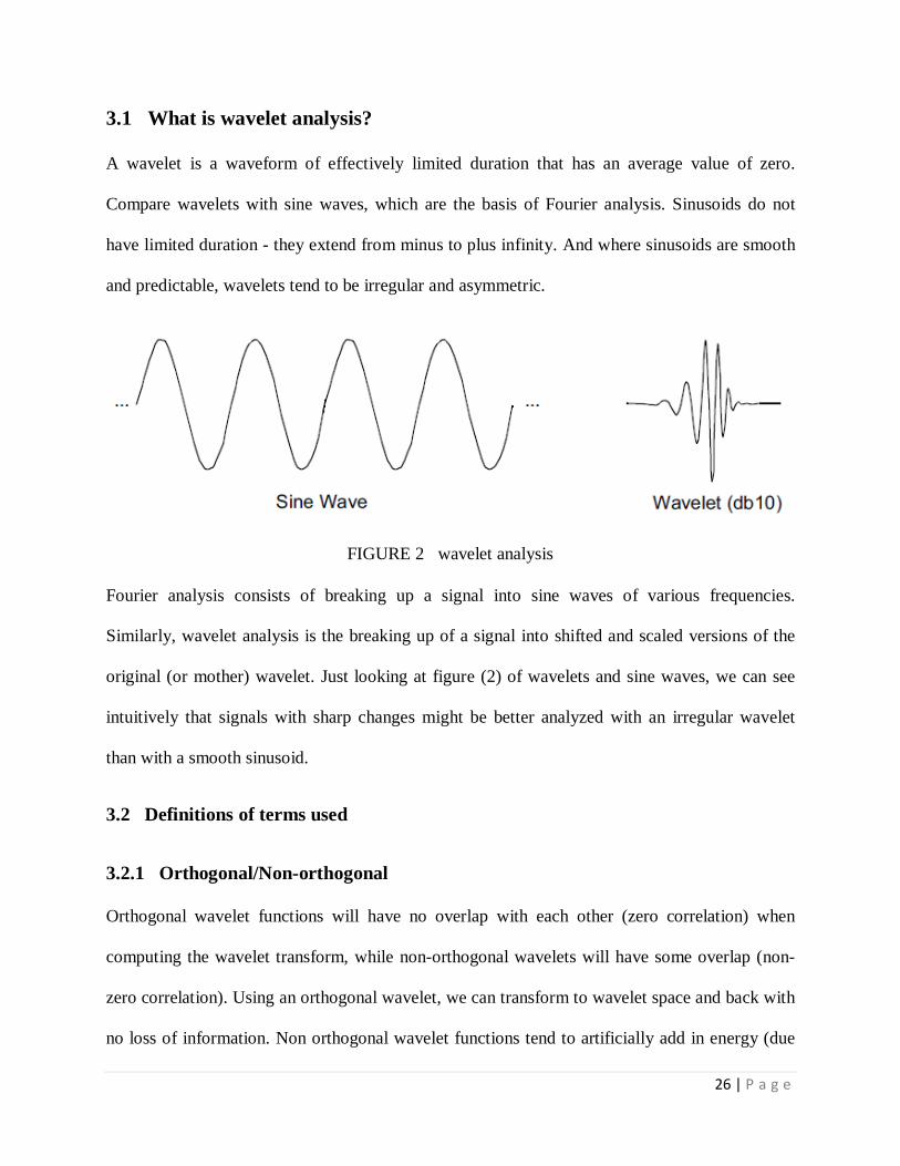
A wavelet is a waveform of effectively limited duration that has an average value of zero.

Compare wavelets with sine waves, which are the basis of Fourier analysis. Sinusoids do not

have limited duration - they extend from minus to plus infinity. And where sinusoids are smooth

and predictable, wavelets tend to be irregular and asymmetric.

FIGURE 2 wavelet analysis

Fourier analysis consists of breaking up a signal into sine waves of various frequencies.

Similarly, wavelet analysis is the breaking up of a signal into shifted and scaled versions of the

original (or mother) wavelet. Just looking at figure (2) of wavelets and sine waves, we can see

intuitively that signals with sharp changes might be better analyzed with an irregular wavelet

than with a smooth sinusoid.

3.2 Definitions of terms used

3.2.1 Orthogonal/Non-orthogonal

Orthogonal wavelet functions will have no overlap with each other (zero correlation) when

computing the wavelet transform, while non-orthogonal wavelets will have some overlap (non-

zero correlation). Using an orthogonal wavelet, we can transform to wavelet space and back with

no loss of information. Non orthogonal wavelet functions tend to artificially add in energy (due

27 | P a g e

to the overlap) and require renormalization to conserve the information. In general, discrete

wavelets are orthogonal while continuous wavelets are non-orthogonal.

3.2.2 Symmetry

It describes the symmetry of the wavelet function about the midpoint. Symmetric Wavelets show

no preferred direction in "time," while asymmetric wavelets give unequal Weighting to different

directions.

3.2.3 Vanishing Moments

An important property of a wavelet function is the number of vanishing moments, which

describes the effect of the wavelet on various signals. A wavelet such as the Daubechies 2 with

vanishing moment=2 has zero mean and zero linear trend. When the Daubechies 2 wavelet is

used to transform a data series, both the mean and any linear trend are filtered out of the series. A

higher vanishing moment implies that more moments (quadratic, cubic, etc.) will be removed

from the signal.

3.2.4 Compact Support

This value measures the effective width of the wavelet function. A narrow wavelet function such

as the Daubechies order 2 (compact support=3) is fast to compute, but the narrowness in “time"

implies a very large width in "frequency." Conversely, wavelets with large compact support such

as the Daubechies order 24 (compact support=47) are smoother, have finer frequency resolution

and are usually more efficient at de-noising.

28 | P a g e

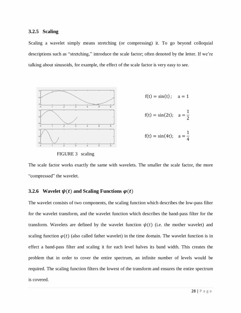
3.2.5 Scaling

Scaling a wavelet simply means stretching (or compressing) it. To go beyond colloquial

descriptions such as “stretching,” introduce the scale factor; often denoted by the letter. If we‟re

talking about sinusoids, for example, the effect of the scale factor is very easy to see.

FIGURE 3 scaling

The scale factor works exactly the same with wavelets. The smaller the scale factor, the more

“compressed” the wavelet.

3.2.6 Wavelet and Scaling Functions

The wavelet consists of two components, the scaling function which describes the low-pass filter

for the wavelet transform, and the wavelet function which describes the band-pass filter for the

transform. Wavelets are defined by the wavelet function (i.e. the mother wavelet) and

scaling function (also called father wavelet) in the time domain. The wavelet function is in

effect a band-pass filter and scaling it for each level halves its band width. This creates the

problem that in order to cover the entire spectrum, an infinite number of levels would be

required. The scaling function filters the lowest of the transform and ensures the entire spectrum

is covered.

29 | P a g e

3.3 Wavelet Transforms:

The word wavelet has been derived from the French world ondelette meaning “small wave” and

coined by Morletand Grossmann [39, 40, 19]. Some contributors include Morlet and Grossmann

[19] for formulation of continuous wavelet transform (CWT), Stromberg [64] for discrete

wavelet transform (DWT), Meyer [43] and Mallat [42] for multi-resolution analysis using

wavelet transform and Daubechies [15] for orthogonal compactly supported wavelets.

3.3.1 Daubechies Wavelet (db)

Named after Ingrid Daubechies, wavelet transform [15] is defined as a tool that cuts up data or

functions or operators in to different frequency components, and then studies each component

with a resolution matched to its scale. The Daubechies wavelets are a family of orthogonal

wavelets defining a discrete wavelet transform and characterized by a maximal number of

vanishing moments for some given support. With each wavelet type of this class, there is a

scaling function (also called father wavelet) which generates an orthogonal multi-resolution

analysis. In the analysis of time signal, the wavelet transform will decompose the signal in to

frequency components and for each of these frequency components.

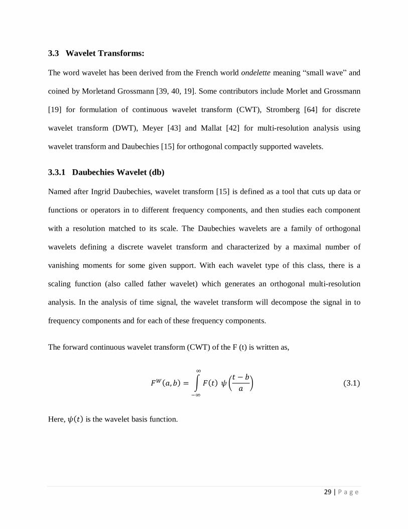
The forward continuous wavelet transform (CWT) of the F (t) is written as,

∫

(

)

Here, is the wavelet basis function.

30 | P a g e

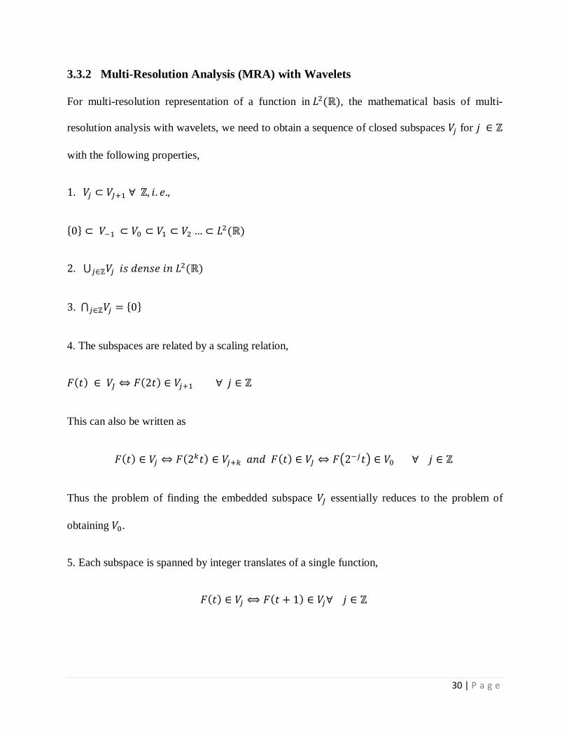
3.3.2 Multi-Resolution Analysis (MRA) with Wavelets

For multi-resolution representation of a function in , the mathematical basis of multi-

resolution analysis with wavelets, we need to obtain a sequence of closed subspaces for

with the following properties,

{ }

{ }

4. The subspaces are related by a scaling relation,

This can also be written as

( )

Thus the problem of finding the embedded subspace essentially reduces to the problem of

obtaining .

5. Each subspace is spanned by integer translates of a single function,

31 | P a g e

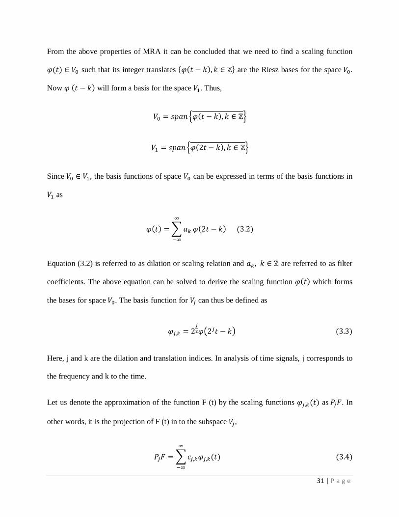
From the above properties of MRA it can be concluded that we need to find a scaling function

such that its integer translates { } are the Riesz bases for the space .

Now will form a basis for the space . Thus,

, -

, -

Since , the basis functions of space can be expressed in terms of the basis functions in

as

∑

Equation (3.2) is referred to as dilation or scaling relation and are referred to as filter

coefficients. The above equation can be solved to derive the scaling function which forms

the bases for space . The basis function for can thus be defined as

( )

Here, j and k are the dilation and translation indices. In analysis of time signals, j corresponds to

the frequency and k to the time.

Let us denote the approximation of the function F (t) by the scaling functions as . In

other words, it is the projection of F (t) in to the subspace ,

∑

32 | P a g e

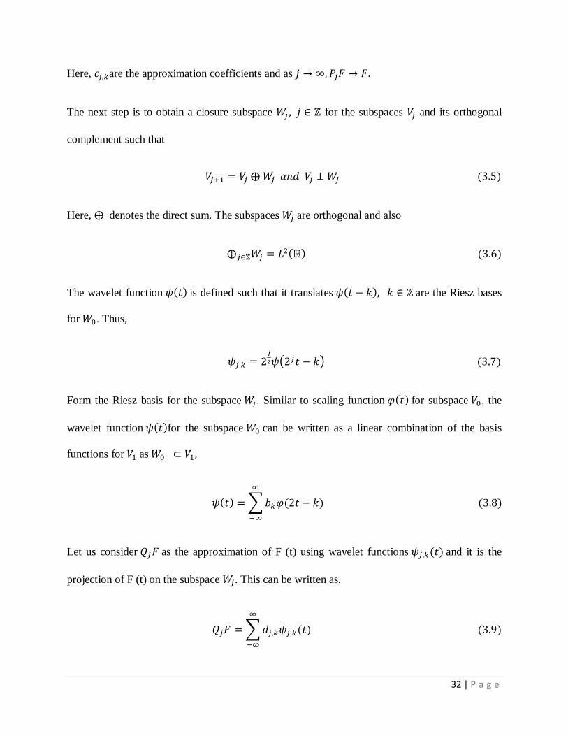
Here, are the approximation coefficients and as

The next step is to obtain a closure subspace for the subspaces and its orthogonal

complement such that

Here, denotes the direct sum. The subspaces are orthogonal and also

The wavelet function is defined such that it translates are the Riesz bases

for . Thus,

( )

Form the Riesz basis for the subspace . Similar to scaling function for subspace , the

wavelet function for the subspace can be written as a linear combination of the basis

functions for as

∑

Let us consider as the approximation of F (t) using wavelet functions and it is the

projection of F (t) on the subspace . This can be written as,

∑

33 | P a g e

Here, are referred as detail coefficients. Now, using equation (3.5) can be written as

Thus, the approximation of F(t) at the higher or refined scale is obtained from the

approximations at the lower scale with lower resolution. This forms the basis of multi-resolution

analysis using wavelets.

3.3.3 Daubechies compactly supported wavelets

It can be summarized from the previous subsection that wavelets form the basis functions

for and any function in can be represented using these bases. Several wavelet

functions are Morlet wavelets, Shanon wavelets, Meyer wavelets, Mexican hat wavelets have

been proposed by the researchers. The choice of wavelet depends on the nature of analysis to be

performed. Daubechies [13, 15] proposed orthogonal compactly supported wavelets referred to

as Daubechies wavelet. There are other compactly supported wavelets like bi-orthogonal spline

(B-spline) wavelets [11, 12], and interpolation wavelets [5, 14].

3.3.4 Construction of Daubechies Compactly Supported Wavelets

The first step in the derivation of these wavelets is to obtain the scaling function from the

scaling or dilation equation given by equation (3.1). The filter coefficients determine the

nature of the wavelet function and for Deaubechies compactly supported wavelets where only a

finite number of filter coefficients are non-zero. is again obtained from using equation

(3.8) and for Daubechies wavelets it can be written as,

34 | P a g e

∑

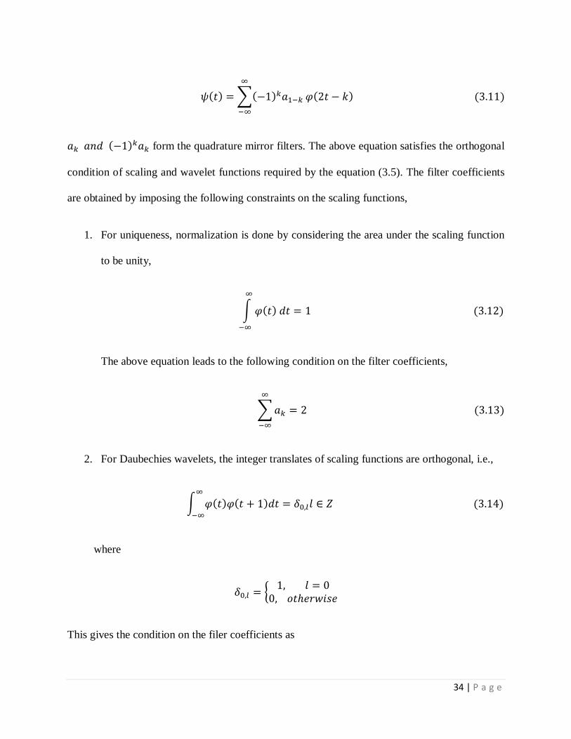
form the quadrature mirror filters. The above equation satisfies the orthogonal

condition of scaling and wavelet functions required by the equation (3.5). The filter coefficients

are obtained by imposing the following constraints on the scaling functions,

1. For uniqueness, normalization is done by considering the area under the scaling function

to be unity,

∫

The above equation leads to the following condition on the filter coefficients,

∑

2. For Daubechies wavelets, the integer translates of scaling functions are orthogonal, i.e.,

∫

where

{

This gives the condition on the filer coefficients as

35 | P a g e

∑

3. The condition on the filter coefficients given by equation (3.13) and (3.15) do not given an

unique set of filter coefficients. For an N coefficients system, the equation (3.13) and (3.15)

provide only

equations required to obtain a unique set of filter coefficients we need some

other conditions to be imposed on the wavelet functions. For Daubechies wavelets, the

conditions are exactly represent polynomial of order M and M = N / 2. Let us consider a

polynomial of order M as

The above polynomial should be exactly represent by an expansion similar to that given

by equation (3.3) for j = 0 and can be written as

∑

Since are orthogonal to the translates of , taking inner product of equation

(3.18) with gives

⟨ ⟩ ∑ ⟨ ⟩

Substituting equation (3.16) in the above equation (3.18) we get

∫

∫

∫

36 | P a g e

The above identity is valid for all . Choosing and all

other gives,

∫

This implies that the first M moments of the wavelet function should be zero. Equation (3.20)

can be written in terms of the filter coefficients after some calculation as

∑

N = 2M determines the order of the Daudechies wavelet and is referred as D4, D6, D8 and

thereafter for N = 4, 6, 8 respectively.

As said before, the scaling functions are obtained by solving recursively the dilation equation

(3.2) which can be expanded for DN as,

Using the compactness criteria of the Daubechies scaling functions between 0 to N – 1 where N

is the order of the DN Daubechies scaling function, the relation given in equation (3.22) can be

written as the following equations,

37 | P a g e

This can also be written as matrix form,

(3.23)

1)-(N

2)-(N

3)-(N

(2)

(1)

(0)

1)-(N

2)-(N

3)-(N

(2)

(1)

(0)

a 0 0 0 0 0

a a a 0 0 0

a a a 0 0 0

0 0 0 a a a

0 0 0 a a a

0 0 0 0 0

1-N

3-N2-N1-N

5-N4-N3-N

234

012

0

a

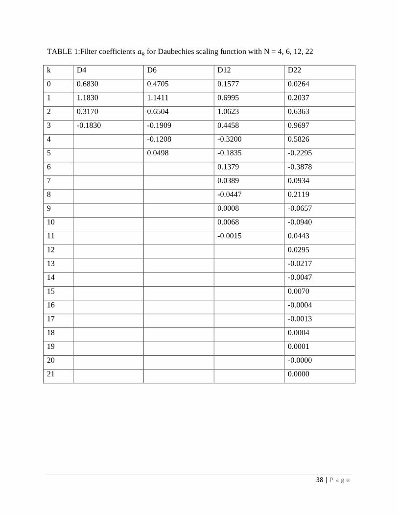
Equation (3.23) possesses eigenvalue problems and can be solved to obtain scaling

functions as the eigenvectors. The matrix B is known as the filter coefficients and can

be solved from equations (3.13), (3.15) and (3.21). The filter coefficients can be obtained using

the MATLAB wavelet toolbox function dfwavf. The filter coefficients for D4, D6, D12 and D22

are show in table 1.

Once the value of scaling functions are obtained at the integer values of t between 0 to N-1,

the values at the points in between the integers can be obtained from the equation (3.2) modified

as

∑

These iterations can be done as many times as required to obtain over a grid of dyadic

points. A unique set of can be obtained through normalization using equation (3.12).The

scaling functions and wavelet functions for Daubechies D4, D6, D12 and D22 with different

vanishing moments are shown in figure (4) and figure (5).

38 | P a g e

TABLE 1:Filter coefficients for Daubechies scaling function with N = 4, 6, 12, 22

k D4 D6 D12 D22

0 0.6830 0.4705 0.1577 0.0264

1 1.1830 1.1411 0.6995 0.2037

2 0.3170 0.6504 1.0623 0.6363

3 -0.1830 -0.1909 0.4458 0.9697

4 -0.1208 -0.3200 0.5826

5 0.0498 -0.1835 -0.2295

6 0.1379 -0.3878

7 0.0389 0.0934

8 -0.0447 0.2119

9 0.0008 -0.0657

10 0.0068 -0.0940

11 -0.0015 0.0443

12 0.0295

13 -0.0217

14 -0.0047

15 0.0070

16 -0.0004

17 -0.0013

18 0.0004

19 0.0001

20 -0.0000

21 0.0000

39 | P a g e

a b

c d

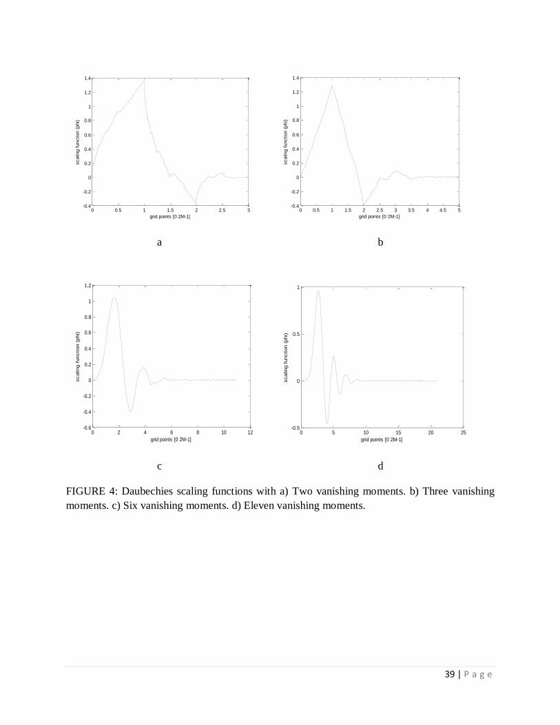
FIGURE 4: Daubechies scaling functions with a) Two vanishing moments. b) Three vanishing

moments. c) Six vanishing moments. d) Eleven vanishing moments.

0 0.5 1 1.5 2 2.5 3-0.4

-0.2

0

0.2

0.4

0.6

0.8

1

1.2

1.4

grid points [0 2M-1]

scaling f

unction (

phi)

0 0.5 1 1.5 2 2.5 3 3.5 4 4.5 5-0.4

-0.2

0

0.2

0.4

0.6

0.8

1

1.2

1.4

grid points [0 2M-1]

scaling f

unction (

phi)

0 2 4 6 8 10 12-0.6

-0.4

-0.2

0

0.2

0.4

0.6

0.8

1

1.2

grid points [0 2M-1]

scaling f

unction (

phi)

0 5 10 15 20 25-0.5

0

0.5

1

grid points [0 2M-1]

scaling f

unction (

phi)

40 | P a g e

a b

c d

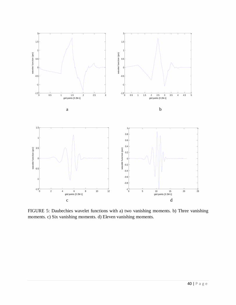
FIGURE 5: Daubechies wavelet functions with a) two vanishing moments. b) Three vanishing

moments. c) Six vanishing moments. d) Eleven vanishing moments.

0 0.5 1 1.5 2 2.5 3-1.5

-1

-0.5

0

0.5

1

1.5

2

grid points [0 2M-1]

wavele

t fu

nction (

psi)

0 0.5 1 1.5 2 2.5 3 3.5 4 4.5 5-1.5

-1

-0.5

0

0.5

1

1.5

2

grid points [0 2M-1]

wavele

t fu

nction (

psi)

0 2 4 6 8 10 12-1.5

-1

-0.5

0

0.5

1

1.5

grid points [0 2M-1]

wavele

t fu

nction (

psi)

0 5 10 15 20 25-1

-0.8

-0.6

-0.4

-0.2

0

0.2

0.4

0.6

0.8

1

grid points [0 2M-1]

wavele

t fu

nction (

psi)

41 | P a g e

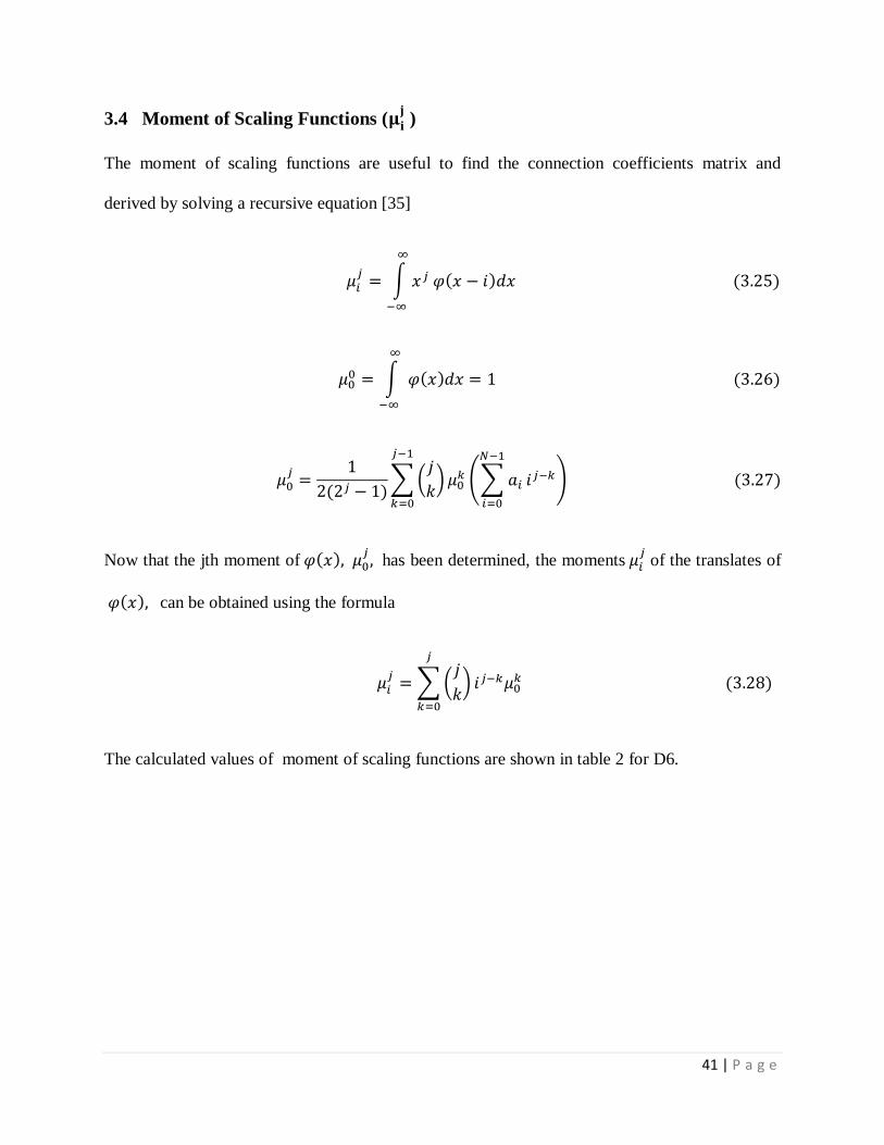
3.4 Moment of Scaling Functions ( )

The moment of scaling functions are useful to find the connection coefficients matrix and

derived by solving a recursive equation [35]

∫

∫

∑(

)

(∑

)

Now that the jth moment of has been determined, the moments

of the translates of

can be obtained using the formula

∑(

)

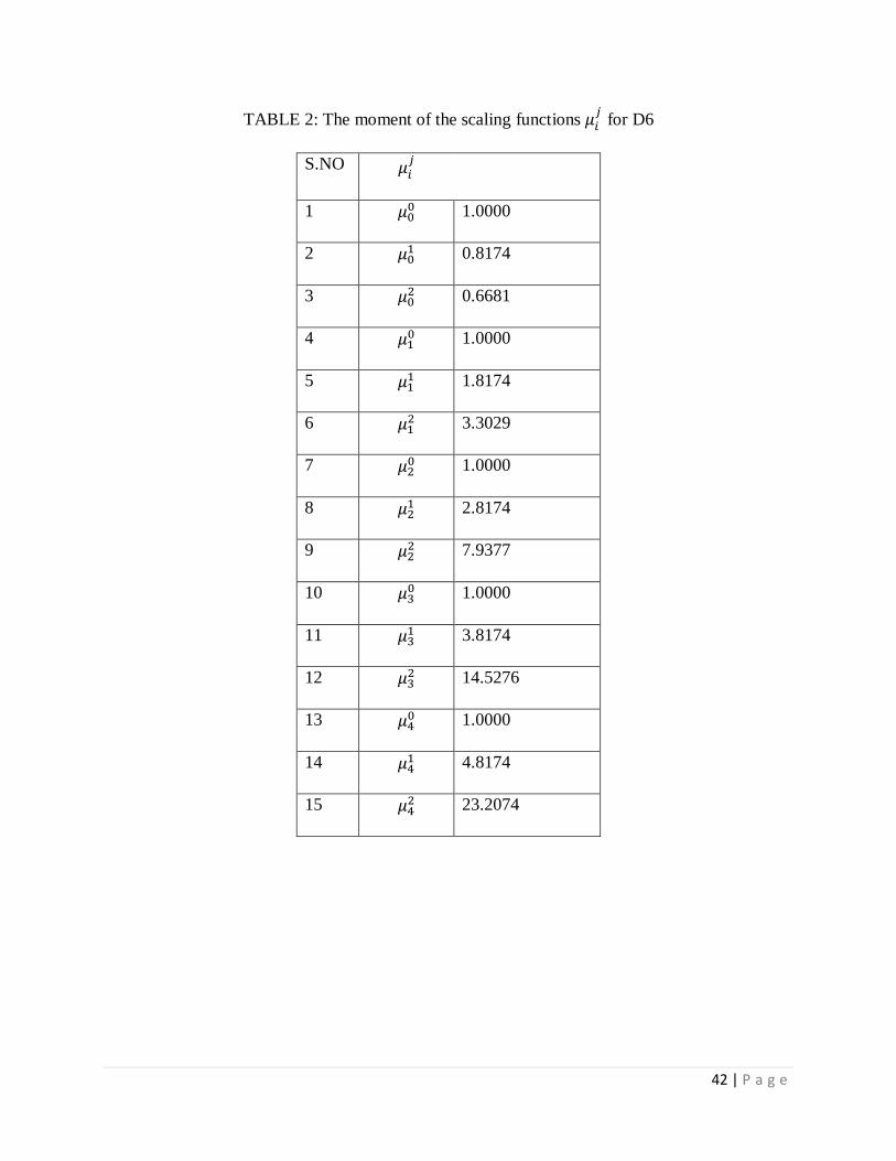
The calculated values of moment of scaling functions are shown in table 2 for D6.

42 | P a g e

TABLE 2: The moment of the scaling functions for D6

S.NO

1 1.0000

2 0.8174

3 0.6681

4 1.0000

5 1.8174

6 3.3029

7 1.0000

8 2.8174

9 7.9377

10 1.0000

11 3.8174

12 14.5276

13 1.0000

14 4.8174

15 23.2074

43 | P a g e

CHAPTER ~ 4

4 Spectral Analysis

44 | P a g e

In the spectral analysis wavelet transforms are used to solve wave propagation problems.

Spectral analysis helps to study the frequency dependent wave characteristics and finally

formulation of Spectral Finite Element Method (SFEM). Spectral Finite Element Method uses

spectral analysis to obtain the local wave behavior for different waveguides and hence the wave

characteristics, namely the Spectrum and the Dispersion relation. These local characteristics are

synthesized to get the global wave behavior. Spectral analysis uses the concepts of Fourier

transform, mostly discrete Fourier transform (DFT) are widely used to represent a field variable

(say displacement) as a finite series involving a set of coefficients, which requires to be

determined based on the boundary conditions of the problems. Spectral analysis enables the

determination of two important wave parameters, namely the wavenumbers and the group

speeds. These parameters are not only required for spectral element formulation, but also to

understand the wave mechanics in a given wave guide. These parameters enable us to know

whether the wave mode is a propagating mode or a damping mode or a combination of these two

(propagation as well as wave amplitude attenuation). If the wave is propagating, the wavenumber

expression will let us know whether it is non-dispersive (i.e. the wave retains its shape as it

propagates) or dispersive (i.e. the wave changes its shape as it propagates).

4.1 Spectrum and Dispersion relations

Here, the two important frequency dependent wave characteristics which are spectrum and

dispersion relations are obtained for a generalized system using Discrete Fourier Transform.

These relations are the frequency variation of the wave parameters termed as wavenumbers and

wave speeds respectively. Here, these parameters are explained using the example of a one-

dimensional second and fourth order partial differential.First considering the second order partial

differential given as,

45 | P a g e

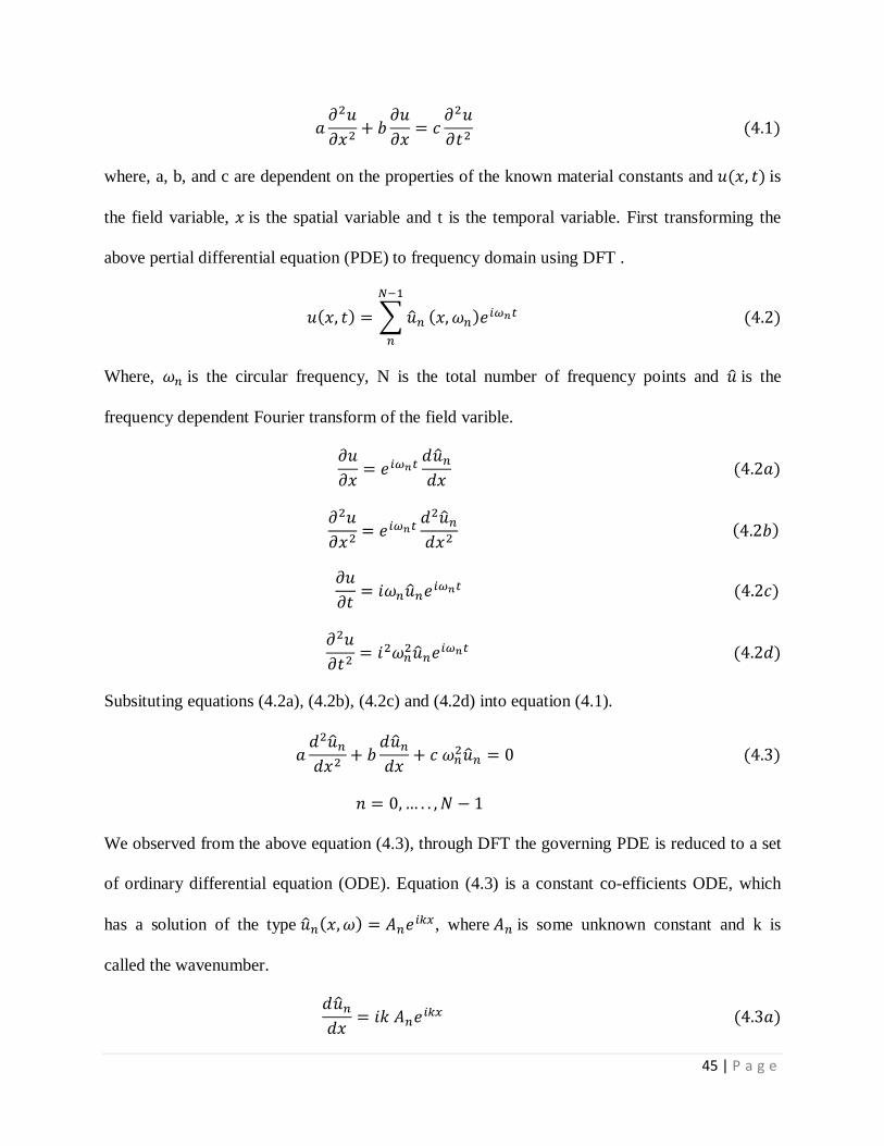
where, a, b, and c are dependent on the properties of the known material constants and is

the field variable, is the spatial variable and t is the temporal variable. First transforming the

above pertial differential equation (PDE) to frequency domain using DFT .

∑

Where, is the circular frequency, N is the total number of frequency points and is the

frequency dependent Fourier transform of the field varible.

Subsituting equations (4.2a), (4.2b), (4.2c) and (4.2d) into equation (4.1).

We observed from the above equation (4.3), through DFT the governing PDE is reduced to a set

of ordinary differential equation (ODE). Equation (4.3) is a constant co-efficients ODE, which

has a solution of the type , where is some unknown constant and k is

called the wavenumber.

46 | P a g e

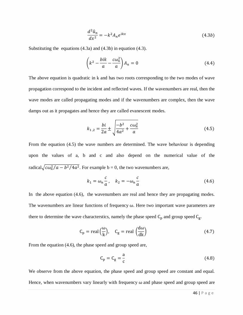
Substituting the equations (4.3a) and (4.3b) in equation (4.3).

.

/

The above equation is quadratic in k and has two roots corresponding to the two modes of wave

propagation correspond to the incident and reflected waves. If the wavenumbers are real, then the

wave modes are called propagating modes and if the wavenumbers are complex, then the wave

damps out as it propagates and hence they are called evanescent modes.

√

From the equation (4.5) the wave numbers are determined. The wave behaviour is depending

upon the values of a, b and c and also depend on the numerical value of the

radical√ ⁄ ⁄ . For example b = 0, the two wavenumbers are,

In the above equation (4.6), the wavenumbers are real and hence they are propagating modes.

The wavenumbers are linear functions of frequency . Here two important wave parameters are

there to determine the wave characterstics, namely the phase speed and group speed

(

) (

)

From the equation (4.6), the phase speed and group speed are,

We observe from the above equation, the phase speed and group speed are constant and equal.

Hence, when wavenumbers vary linearly with frequency and phase speed and group speed are

47 | P a g e

equal and constant, then the wave propagates retains its shape called Non-dispersive waves. If

the wavenumbers vary non-linearly with frequency and phase speed and group speed are not

constant but will be functions of frequency i.e. each frequency components travels with different

speed as a result, the wave changes its shape as it propagates are called dispersive waves.

Next considering the equation (4.5) with all the constants nonzero. The wavenumbers no longer

varies linearly with the frequency. Hence, it can be expected to have dispersive behavior of the

waves and the level of dispersion will depend upon the numerical value of the radical. There can

be following three cases

Case 1.

, then the radical will be a complex number and hence all the wavenumbers

will be complex. Hence, the wave modes are called evanescent or a damping mode.

Case 2.

, the value of the radical will be positive and real and hence the wavenumber

will have both real and imaginary parts i.e. , for this case the phase speed and group

speed are,

√ ⁄ ⁄

√ ⁄ ⁄

In the above equations the phase speed and group speed are not same and hence the nature of

wave is dispersive. To get the Non-dispersive wave, subsituting b = 0 in equation (4.10).

48 | P a g e

Case 3.

, If the values of the radical will be zero and hence the wavenumber is purely

imaginary indicating that the wave mode is a damping mode. Here, the interesting point is to find

the transition frequency at which the propagating mode becomes evanescent or a damping mode.

This can be obtained by equating the radical to zero. The frequency of transition is given as,

√

Once the wavenumbers are obtained, the solution to the governing wave equation (4.3) in the

frequency domain can be written as (for b = 0)

√

where represent the incident wave coefficient and represent the reflected wave coefficient.

For SFEM, the solution of the governing equation is the starting point in the frequency domain.

It can be seen that how the values of the constants in the governing differential equation play an

important role in dictating the type of wave propagation.

Now considering the fourth order partial differential equation as

Here, w is the field variable and A,B,C are material constants.

Now assuming the spectral form of solution to the field variable given as

∑

where, is the circular frequency, N is the total number of frequency points and is the

frequency dependent Fourier transform of the field varible.

49 | P a g e

Subsituting equations (4.15a), (4.15b), (4.15c) and (4.15d) into equation (4.15).

We observed from the equation (4.16), through DFT the governing PDE is reduced to a set of

ordinary differential equation (ODE). Equation (4.16) is a constant co-efficients ODE, which has

a solution of the type , where is some unknown constant and k is called the

wavenumber.

Substituting the equations (4.16a) and (4.16b) in equation (4.16).

.

/

(

)

50 | P a g e

The above equation is quadratic in k is a fourth order equation corresponding to the four modes

of wave propagation two are for the incident and other two for the reflected waves. Also, the

wave type is dependend upon the numerical value of

.

Let assuming

for this case the solution of equation (4.19) will give the following

wavenumbers as,

In the equation (4.20), and are the propagating modes while and are the damping or

evanescent modes. From the above equation we conclude that the wavenumbers are non-linear

functions of the frequency and the mature of waves are dispersive. Also from the above

experssion the phase and group speeds for the propagating modes using equations (4.7) and

(4.8) are determined.

Next, considering the case when

. For this case, the characteristic equation and the

wavenumbers are given as

[

√

√ ] [

√

√ ]

[

√

√ ] [

√

√ ]

We abserve from the above equation, that the change of sign of

has caused completely

changed wave behavior. We find that all the wavenumbers have both real and the imaginary

parts and hence all the modes are propagating as well as attenuating. Also the initial evanescent

mode, after a certain frequency, becomes a propagating mode, giving a completely different

51 | P a g e

wave behavior. The frequency at which this transition takes place is called the cut-off frequency.

The cut-off frequency can be obtained if we equate

to zero,

√

The solution of the fourth-order governing equation in the frequency domain (equation (4.16))

can be written as

Here, and are the incident wave coefficients and and are the reflected wave

coefficients. These can be determined based on the boundry conditions of the problems.

From the above discussion, the direct output of spectral analysis are the spectrum relation, which

is a plot of the wavenumber variation with frequency, and dispersion relations, which is a plot of

the speed against frequency. These relations are absolute necessary for the spectral finite element

formulation.

4.2 Computations of wavenumbers and wave amplitudes

The wavenumbers are obtained as a function of frequency by solving second and fourth order

polynomial equations. The determination of wavenumbers are not so straight forward for

structures with higher complexities. For one-dimensional structures problems arises when the

governing equation is a set of coupled PDEs. In order to handle to such problems, generalized

and computationally implementable methods have been proposed [22] to calculate the

wavenumbers and wave amplitudes. The two different methods to solve the problems are based

on singular value decomposition (SVD) and polynomial eigenvalue problem (PEP) methods. The

methods are explained briefly in the following subsections using the example of a Extended

Euler-Bernoulli beam.

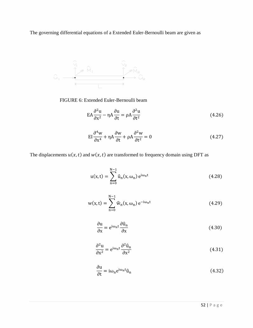
52 | P a g e

The governing differential equations of a Extended Euler-Bernoulli beam are given as

FIGURE 6: Extended Euler-Bernoulli beam

The displacements and are transformed to frequency domain using DFT as

∑

∑

53 | P a g e

The above equations are substituting into equations (4.26) and (4.27)

Assuming the solution of the above equations as

54 | P a g e

4.2.1 Singular value decomposition (SVD)

In this method the above equations (4.44) and (4.45) are writing in matrix form as

[

] {{

}

Here considering damping zero

[

] {{

}

Here, the k‟s are the latent roots of the above equation, which satisfy the

conditions ( ) [ ]. For each solution of k, there is at least one non-trivial solution

for C which is known as the latent eigenvector. To find the latent roots, the determined is

expanded in a polynomial of k, p(k), and solved by the companion matrix method. The

companion matrix L(p), corresponding to p(k) is formed as

(4.49)

- - -

1 0 0 0

0 1 0 0

0 0 1 0

)(

121-m

m

pL

Where p(k) is given as

55 | P a g e

The eigenvalue of are the roots of , which are obtained using standard techniques.

Once the eigenvalues are obtained they are used to obtain the eigenvectors. The eigenvectors are

the element of the null space of W (k) and the eigenvalues make this null space non-trivial by

rendering W(k) singular. The computation of the eigenvectors is equivalent to computation of the

null space of a matrix. For this purpose the SVD method is most effective. U, V and the diagonal

matrix S as , where H is the Hermitian conjugate. S is the singular value matrix. For

singular matrices, one or more of the singular values will be zero and the required property of the

unitary matrix V is that the columns of V corresponding to zero singular values are the elements

of the null space of A.

4.3 Spectral Finite Element Method (SFEM)

Spectral finite element method is highly suitable for wave propagation analysis as it is in

frequency domain. The SFEM in brief is a FE method in the frequency domain which is the main

difference between SFEM and FEM.

Finite element method is based on assumed polynomial for displacement. These assumed

displacement polynomials are forced to satisfy the weak form of the governing differential

equation, which would yield two different matrices namely the stiffness matrix and the mass

matrix. These elemental matrices are assembled to obtain the global stiffness and mass matrices.

The assemble process ensures equilibrium of forces between the adjacent elements. This

procedure will give the discretized form of the governing equation as

[ ]{ } [ ]{ } [ ]{ } { }

Where [ ] and [ ] are the global mass and stiffness matrix and { }, { } and { } are the

acceleration, velocity and displacement vectors.

56 | P a g e

The above equation is an ODE in time. These equations are solved by the method of mode

superposition. As mentioned earlier, the mode superposition method of solution cannot be used

for wave propagation analysis. The methods which can be implemented are the time marching

schemes [6] which can be either be the explicit or implicit methods. Normally the explicit

methods are used for the transient dynamic problem of wave propagation. The solution of the

dynamics equation will give displacement, velocity and acceleration histories. The solution time

being directly proportional to the number of degree of freedoms, the computational time of such

a scheme is very high for wave propagation problems.

On the other hand SFEM uses in most cases the exact solution to the wave equation as its

interpolating function. The exact solution will have wave coefficients corresponding to the

incident and reflected wave components. If we model for an infinite domain, then the reflected

components can be dropped from the interpolating functions are called throw-off elements. This

is a great advantage that SFEM have over FEM. Using the interpolation functions for the

displacements; the dynamic element stiffness matrix is formulated. The steps involved in the

analysis using SFEM are as follows. First the given function is transformed to the frequency

domain using the forward FFT. While doing we need to choose the time sampling rate and

number of FFT points to decide on the analysis time window. Care should be taken to see that

the chosen window is good enough to avoid wraparound problems [16]. The FFT output will

yield the frequency, the real and imaginary part of the forcing function, which are stored

separately. Over a big frequency loop, the elemental stiffness matrix is generated, assembled and

solved as in the case of conventional FEM. The solution process is first performed for a unit

impulse, which directly yields the Frequency Response Function (FRF). The FRF is then

57 | P a g e

convolved with the load to get the required output in the frequency domain. This output is then

transformed to the time domain using the inverse FFT.

There are many advantages that SFEM has over conventional FEM. The SFEM can produce

results in both the time and frequency domain in a single analysis. Obtaining the FRF is a big

advantage of the SFEM. This enables one to solve inverse problems such as the force or the

system identification problems.

58 | P a g e

CHAPTER ~ 5

5 Wavelet Spectral Finite Element

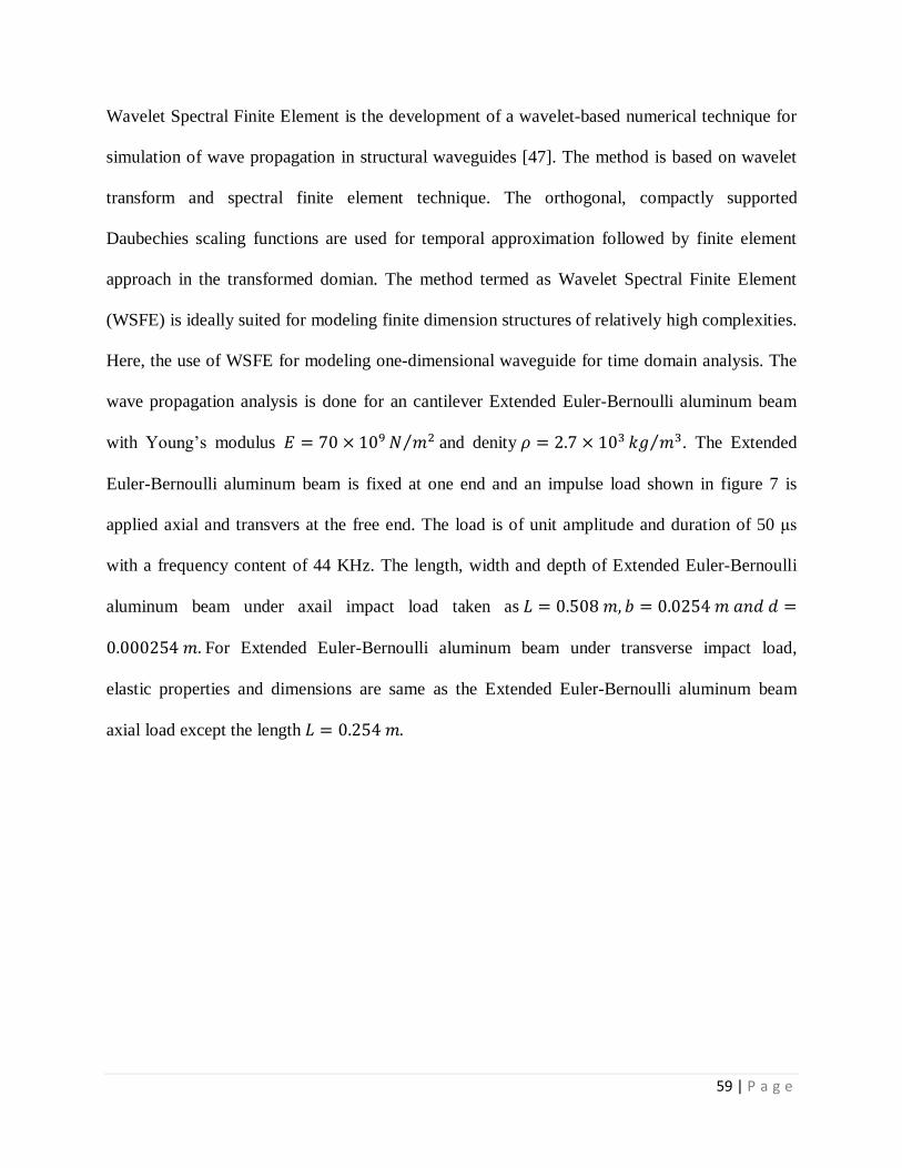
59 | P a g e

Wavelet Spectral Finite Element is the development of a wavelet-based numerical technique for

simulation of wave propagation in structural waveguides [47]. The method is based on wavelet

transform and spectral finite element technique. The orthogonal, compactly supported

Daubechies scaling functions are used for temporal approximation followed by finite element

approach in the transformed domian. The method termed as Wavelet Spectral Finite Element

(WSFE) is ideally suited for modeling finite dimension structures of relatively high complexities.

Here, the use of WSFE for modeling one-dimensional waveguide for time domain analysis. The

wave propagation analysis is done for an cantilever Extended Euler-Bernoulli aluminum beam

with Young‟s modulus ⁄ and denity ⁄ . The Extended

Euler-Bernoulli aluminum beam is fixed at one end and an impulse load shown in figure 7 is

applied axial and transvers at the free end. The load is of unit amplitude and duration of 50 μs

with a frequency content of 44 KHz. The length, width and depth of Extended Euler-Bernoulli

aluminum beam under axail impact load taken as

For Extended Euler-Bernoulli aluminum beam under transverse impact load,

elastic properties and dimensions are same as the Extended Euler-Bernoulli aluminum beam

axial load except the length

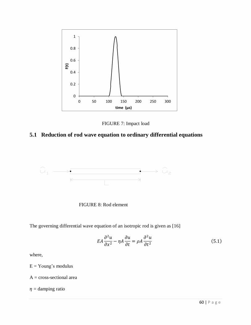
60 | P a g e

FIGURE 7: Impact load

5.1 Reduction of rod wave equation to ordinary differential equations

FIGURE 8: Rod element

The governing differential wave equation of an isotropic rod is given as [16]

where,

E = Young‟s modulus

A = cross-sectional area

= damping ratio

0

0.2

0.4

0.6

0.8

1

0 50 100 150 200 250 300

F(t)

time (µs)

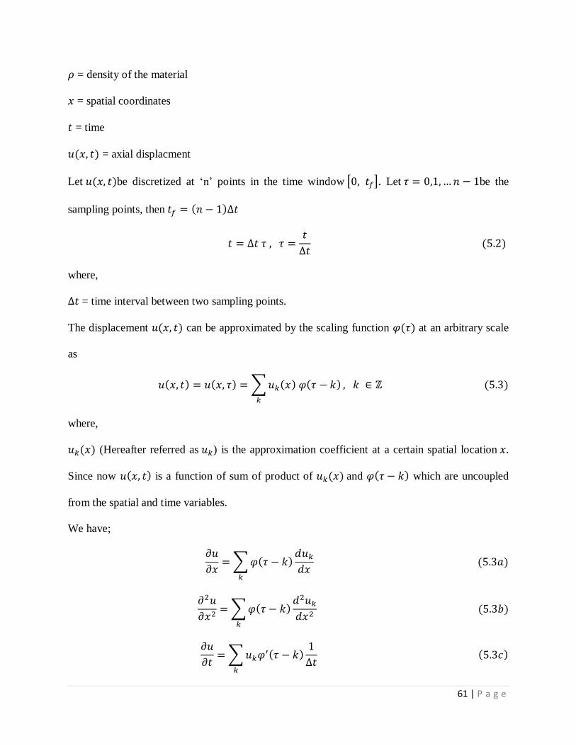
61 | P a g e

= density of the material

= spatial coordinates

= time

= axial displacment

Let be discretized at „n‟ points in the time window [ ]. Let be the

sampling points, then

where,

= time interval between two sampling points.

The displacement can be approximated by the scaling function at an arbitrary scale

as

∑

where,

(Hereafter referred as ) is the approximation coefficient at a certain spatial location .

Since now is a function of sum of product of and which are uncoupled

from the spatial and time variables.

We have;

∑

∑

∑

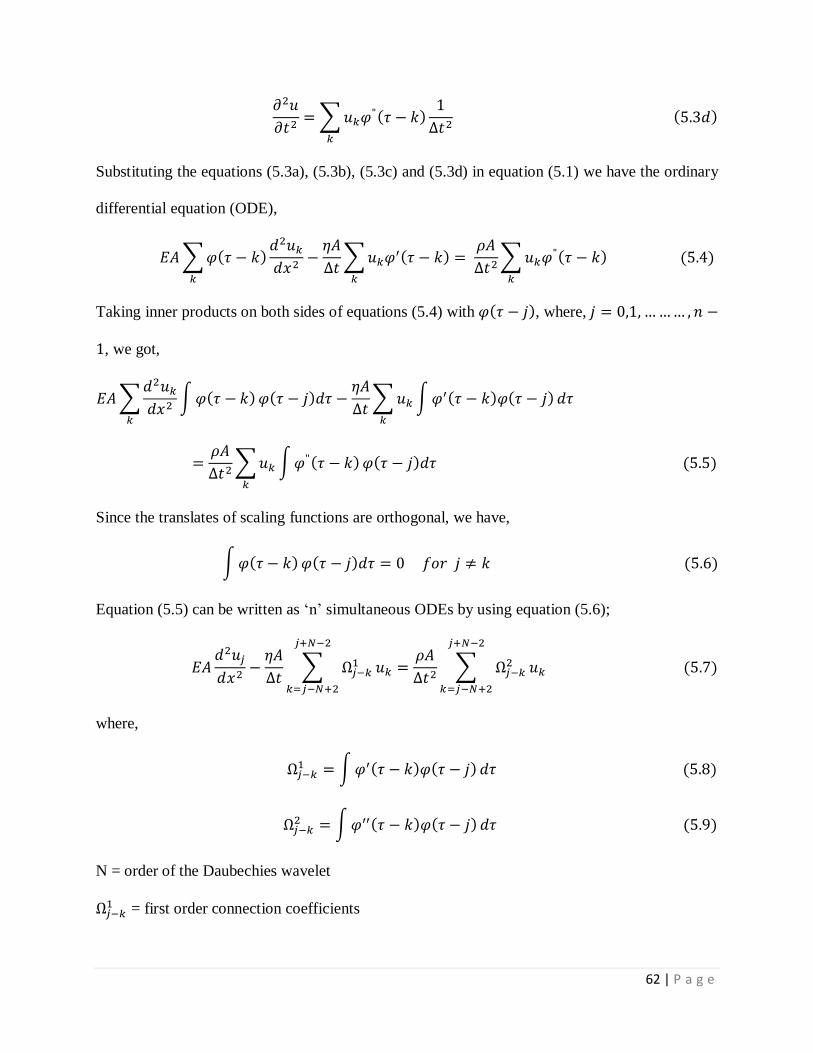
62 | P a g e

∑

Substituting the equations (5.3a), (5.3b), (5.3c) and (5.3d) in equation (5.1) we have the ordinary

differential equation (ODE),

∑

∑

∑

Taking inner products on both sides of equations (5.4) with , where,

, we got,

∑

∫

∑ ∫

∑ ∫

Since the translates of scaling functions are orthogonal, we have,

∫

Equation (5.5) can be written as „n‟ simultaneous ODEs by using equation (5.6);

∑

∑

where,

∫

∫

N = order of the Daubechies wavelet

= first order connection coefficients

63 | P a g e

= second order connection coefficients

For compactly supported wavelets, ,

are nonzero only in the interval

From the equation (5.7);

∑ (

)

The values of the connection coefficients for D22 first and second order are shown in table 3.

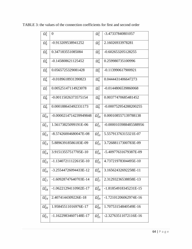
64 | P a g e

TABLE 3: the values of the connection coefficients for first and second order

0

-3.47337840801057

-0.913209538941252

2.16026933978281

0.347183551085084

-0.602653205128255

-0.145808621125452

0.259980735100996

0.0565725329081428

-0.113990617900921

-0.0189618931390823

0.0444431406647273

0.00525147114923078

-0.0144806539860068

-0.00115026373575154

0.00377470685481452

0.000188643492331173

-0.000752954288200255

-0.0000214714239949848

0.000108557139788138

1.56173825099191E-06

-0.0000103988485588956

-8.57426004680047E-08

5.55791376315321E-07

5.88963918586183E-09

3.72688117300783E-09

3.91513557517705E-10

-5.40977631679387E-09

-1.13407211122615E-10

4.73721978304495E-10

-3.25544726094433E-12

3.16562432692258E-11

-1.60928747640703E-14

2.31293236538858E-13

-1.06221294110902E-17

-1.81854918345231E-15

2.4074144309226E-18

-1.72101206062974E-16

1.95845511016976E-17

1.70753154840549E-16

-1.16229834607148E-17

-2.32763511072116E-16

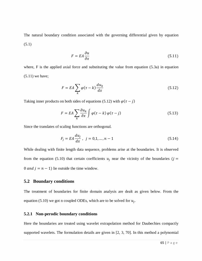
65 | P a g e

The natural boundary condition associated with the governing differential given by equation

(5.1)

where, F is the applied axial force and substituting the value from equation (5.3a) in equation

(5.11) we have;

∑

Taking inner products on both sides of equations (5.12) with

∑

∫

Since the translates of scaling functions are orthogonal.

While dealing with finite length data sequence, problems arise at the boundaries. It is observed

from the equation (5.10) that certain coefficients near the vicinity of the boundaries

lie outside the time window.

5.2 Boundary conditions

The treatment of boundaries for finite domain analysis are dealt as given below. From the

equation (5.10) we got n coupled ODEs, which are to be solved for .

5.2.1 Non-perodic boundary conditions

Here the boundaries are treated using wavelet extrapolation method for Daubechies compactly

supported wavelets. The formulation details are given in [2, 3, 70]. In this method a polynomial

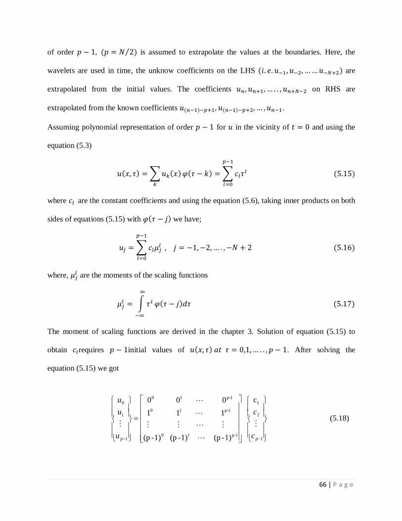
66 | P a g e

of order ⁄ is assumed to extrapolate the values at the boundaries. Here, the

wavelets are used in time, the unknow coefficients on the LHS are

extrapolated from the initial values. The coefficients on RHS are

extrapolated from the known coefficients .

Assuming polynomial representation of order for in the vicinity of and using the

equation (5.3)

∑

∑

where are the constant coefficients and using the equation (5.6), taking inner products on both

sides of equations (5.15) with we have;

∑

where, are the moments of the scaling functions

∫

The moment of scaling functions are derived in the chapter 3. Solution of equation (5.15) to

obtain requires initial values of . After solving the

equation (5.15) we got

(5.18)

c

1)-(p 1)-(p 1)-(p

1 1 1

0 0 0

1

2

1

1-p10

1-p10

1-p10

1

1

0

pp c

c

u

u

u

67 | P a g e

(5.19)

u

1)-(p 1)-(p 1)-(p

1 1 1

0 0 0

1

1

0

1

1-p10

1-p10

1-p10

1

2

1

pp u

u

c

c

c

The values of obtained in terms of the initial values. The unknown coefficient

, we have;

(5.20)

c

1

1

0

1

2N-

1

2N-

0

2

1-P

2-

1

2-

0

2

1-P

1-

1

1-

0

1

2

2

1

pP

NNc

c

u

u

u

The equation (5.19) subsituting into equation (5.20), we have

(5.21)

u

1)-(p 1)-(p 1)-(p

1 1 1

0 0 0

1

1

0

1

1-p10

1-p10

1-p10

1

2N-

1

2N-

0

2

1-P

2-

1

2-

0

2

1-P

1-

1

1-

0

1

2

2

1

pP

NNu

u

u

u

u

The unknown coefficients at the RHS boundary are determining by assuming same polynomial

representation as

∑

Equation (5.22) writing matrix form as

(5.23)

c

u

1

1

0

1

1

1

1-

0

1

1

1

1

1p-

0

1

1-p

p-

10

1

21

11-n

pp

p

pp

pp

n

pn

p

c

c

u

u

68 | P a g e

From the above equation (5.23), the values areobtained, we have;

(5.24)

u

c

1

21

11-n

1

1

1

1-

0

1

1

1

1

1p-

0

1

1-p

p-

10

1

1

0

n

pn

p

p

p

pp

pp

p u

u

c

c

To get the unknown coefficients at the RHS, subsittiting into

equation (5.22), we have;

(5.25)

c

u

1

1

0

1-p

3-N

1

3-N

0

3-N

1-p

1

1

1

0

1

1-p

0

1

0

0

0

2-N1-n

1

p

n

n

c

cu

u

Equation (5.24) substituting into equation (5.25) and finally, these coefficients are substituted

into equation (5.10) and the systems of ODEs are written in matrix form, we have;

{

} (

) { }

Where, and are the first and second order connection coefficient matrices.

It observed from the above process, the connection coefficient matrices are independent of the

problem and depend only on order of the Daubechies wavelet used, i.e. N

5.3 Decoupling using eigenvalue analysis

It can be seen from the above derivations that the wavelet coefficients of first and second

derivatives can be obtained as

{ } { }

{ } { }

The second derivative can also be written as

69 | P a g e

{ } { }

Substituting equation (5.27) into equation (5.29), we have;

{ } [ ] { }

The second order connection coefficient matrix can be determined independently [4], it can be

also be written as

[ ]

The above modification is done as this helps in imposing the initial conditions for non-perodic

solution. Thus the equation (5.26) can be written as

{

} (

[ ] ) { }

In wavelet spectral finite element, the reduced ODEs are coupled, however the system of

equation can be decoupled by diagonalizing the connection coefficient matrix. This can be done

by eigenvalue analysis of the matrix as

Where is the eigenvector matrix of and is the diagonal matrix containing corresponding

eigenvalues From equation (5.31), can be written as

Where is a diagonal matrix with diagonal terms This eigenvalue analysis is costly but can

be done once and stored as it is completely independent of the problem.

The ODEs obtained by decoupling the equation (5.32) can be written as

(

)

where,

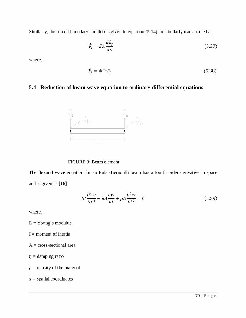
70 | P a g e

Similarly, the forced boundary conditions given in equation (5.14) are similarly transformed as

where,

5.4 Reduction of beam wave equation to ordinary differential equations

FIGURE 9: Beam element

The flexural wave equation for an Eular-Bernoulli beam has a fourth order derivative in space

and is given as [16]

where,

E = Young‟s modulus

I = moment of inertia

A = cross-sectional area

= damping ratio

= density of the material

= spatial coordinates

71 | P a g e

= time

= tranverse displacment

Let be discretized at „n‟ points in the time window [ ]. Let be the

sampling points, then

where,

= time interval between two sampling points.

The displacement can be approximated by the scaling function at an arbitrary scale

as

∑

where,

(Hereafter referred as ) is the approximation coefficient at a certain spatial location .

Since now is a function of sum of product of and which are uncoupled

from the spatial and time variables

We have;

∑

∑

∑

∑

72 | P a g e

∑

∑

Substituting the equations (5.41a), (5.41b), (5.41c), (5.41d), (5.41e) and (5.41f) in equation

(5.39) we have the ordinary differential equation (ODE),

∑

∑

∑

Taking inner products on both sides of equations (5.42) with , Where,

, we get,

∑

∫

∑ ∫

∑ ∫

Since the translates of scaling functions are orthogonal, we have,

∫

Equation (5.43) can be written as „n‟ simultaneous ODEs by using equation (5.44);

∑

∑

where,

∫

∫

N = order of the Daubechies wavelet

73 | P a g e

= first order connection coefficients

= second order connection coefficients

For compactly supported wavelets, ,

are nonzero only in the interval

From the equation (5.45);

∑ (

)

The natural boundary condition associated with the governing differential given by equation

(5.39)

Where, M and V are the applied moment and transverse force and substituting the value from

equations (5.41b) and (5.41c) in equations (5.49) and (5.50) we have;

∑

∑

Taking inner products on both sides of equations (5.51) and (5.52) with , we have;

∑

∫

∑

∫

Since the translates of scaling functions are orthogonal.

74 | P a g e

While dealing with finite length data sequence, problems arise at the boundaries. It observed

from the equation (5.48) that certain coefficients near the vicinity of the boundaries

lie outside the time window.

5.5 Boundary conditions

The treatment of boundaries for finite domain analysis. From the equation (5.48) we got n

coupled ODEs, which are to be solved for .

5.5.1 Non-perodic boundary conditions

Here the boundaries are treating using wavelet extrapolation method for Daubechies compactly

supported wavelets. The formulation details are given in [2, 3, 70]. In this method apolynomial

of order ⁄ is assumed to extrapolate the values at the boundaries. Here, the

wavelets are used in time, the unknow coefficients on the LHS are

extrapolated from the initial values. The coefficients on RHS are

extrapolated from the known coefficients .

Assuming polynomial representation of order for in the vicinity of and using the

equation (5.41)

∑

∑

Where are the constant coefficients and using the equation (5.44), taking inner products on

both sides of equations (5.57) with we have;

75 | P a g e

∑

Where, are the moments of the scaling functions

∫

The moment of scaling functions are derived in the chapter 3. Solution of equation (5.57) to

obtain requires initial values of . After solving the

equation (5.57) we got

(5.60)

c

1)-(p 1)-(p 1)-(p

1 1 1

0 0 0

1

1

0

1-p10

1-p10

1-p10

1

1

0

pp c

c

w

w

w

(5.61)

w

1)-(p 1)-(p 1)-(p

1 1 1

0 0 0

1

1

0

1

1-p10

1-p10

1-p10

1

1

0

pp w

w

c

c

c

The values of obtained in terms of the initial values. The unknown coefficient

, we have;

(5.62)

c

1

1

0

1

2N-

1

2N-

0

2

1-P

2-

1

2-

0

2

1-P

1-

1

1-

0

1

2

2

1

pP

NNc

c

w

w

w

The equation (5.19) subsituting into equation (5.20), we have

76 | P a g e

(5.63)

u

1)-(p 1)-(p 1)-(p

1 1 1

0 0 0

1

1

0

1

1-p10

1-p10

1-p10

1

2N-

1

2N-

0

2

1-P

2-

1

2-

0

2

1-P

1-

1

1-

0

1

2

2

1

pP

NNu

u

w

w

w

The unknown coefficients at the RHS boundary are determining by assuming same polynomial

representation as

∑

Equation (5.64) writing matrix form as

(5.65)

c

w

1

1

0

1

1

1

1-

0

1

1

1

1

1p-

0

1

1-p

p-

10

1

21

11-n

pp

p

pp

pp

n

pn

p

c

c

w

w

From the above equation (5.65), the values are obtained, we have;

(5.66)

w

c

1

21

11-n

1

1

1

1-

0

1

1

1

1

1p-

0

1

1-p

p-

10

1

1

0

n

pn

p

p

p

pp

pp

p w

w

c

c

To get the unknown coefficients at the RHS, subsittiting into

equation (5.64), we have;

(5.67)

c

w

1

1

0

1-p

3-N

1

3-N

0

3-N

1-p

1

1

1

0

1

1-p

0

1

0

0

0

2-N1-n

1

p

n

n

c

cw

w

77 | P a g e

Equation (5.66) substituting into equation (5.67) and finally, these coefficients are substituted

into equation (5.52) and the systems of ODEs are written in matrix form, we have;

{

} (

) { }

Where, and are the first and second order connection coefficient matrices.

It observed from the above process, the connection coefficient matrices are independent of the

problem and depend only on order of the Daubechies wavelet used, i.e. N

5.6 Decoupling using eigenvalue analysis

It can be seen from the above derivations that the wavelet coefficients of first and second

derivatives can be obtained as

{ } { }

{ } { }

The second derivative can also be written as

{ } { }

Substituting equation (5.69) into equation (5.71), we have;

{ } [ ] { }

The second order connection coefficient matrix can be determined independently [4], it can be

also be written as

[ ]

The above modification is done as this helps in imposing the initial conditions for non-perodic

solution. Thus the equation (5.68) can be written as

{

} (

[ ] ) { }

78 | P a g e

In wavelet spectral finite element, the reduced ODEs are coupled, however the system of

equation can be decoupled by diagonalizing the connection coefficient matrix. This can be done

by eigenvalue analysis of the matrix as

where is the eigenvector matrix of and is the diagonal matrix containing corresponding

eigenvalues From equation (5.73), can be written as

where is a diagonal matrix with diagonal terms This eigenvalue analysis is costly but can

be done once and stored as it is completely independent of the problem.

The ODEs obtained by decoupling the equation (5.74) can be written as

(

)

where,

Similarly, the forced boundary conditions given in equation (5.56) are similarly transformed as

79 | P a g e

CHAPTER ~ 6

6 Wavelet Spectral Finite

Element Formulation

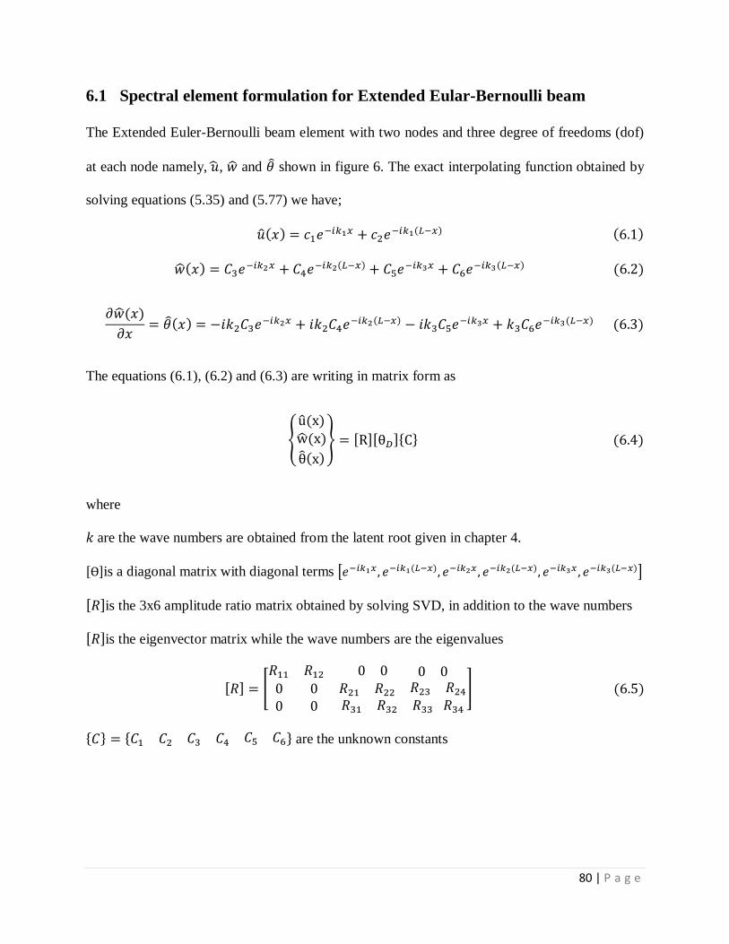
80 | P a g e

6.1 Spectral element formulation for Extended Eular-Bernoulli beam

The Extended Euler-Bernoulli beam element with two nodes and three degree of freedoms (dof)

at each node namely, , and shown in figure 6. The exact interpolating function obtained by

solving equations (5.35) and (5.77) we have;

The equations (6.1), (6.2) and (6.3) are writing in matrix form as

{

} [ ][ ]{ }

where

are the wave numbers are obtained from the latent root given in chapter 4.

[ ]is a diagonal matrix with diagonal terms [ ]

[ ]is the 3x6 amplitude ratio matrix obtained by solving SVD, in addition to the wave numbers

[ ]is the eigenvector matrix while the wave numbers are the eigenvalues

[ ] [

]

{ } { } are the unknown constants

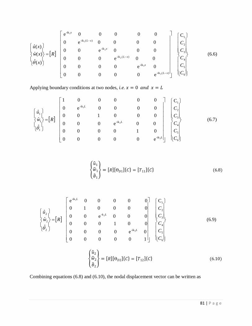
81 | P a g e

(6.6)

C

e 0 0 0 0 0

0 e 0 0 0 0

0 0 e 0 0 0

0 0 0 e 0 0

0 0 0 0 e 0

0 0 0 0 0 e

)(ˆ

)(ˆ

)(ˆ

6

5

4

3

2

1

)(ik-

ik-

)(ik-

ik-

)(ik-

-ik

3

3

2

2

1

1

C

C

C

C

C

R

x

xw

xu

xL

x

xL

x

xL

x

Applying boundary conditions at two nodes, i.e.

(6.7)

C

e 0 0 0 0 0

0 1 0 0 0 0

0 0 e 0 0 0

0 0 0 1 0 0

0 0 0 0 e 0

0 0 0 0 0 1

ˆ

ˆ

ˆ

6

5

4

3

2

1

ik-

ik-

ik-

1

1

1

3

2

1

C

C

C

C

C

Rw

u

L

L

L

{

} [ ][ ]{ } [ ]{ }

(6.9)

C

1 0 0 0 0 0

0 e 0 0 0 0

0 0 1 0 0 0

0 0 0 e 0 0

0 0 0 0 1 0

0 0 0 0 0 e

ˆ

ˆ

ˆ

6

5

4

3

2

1

ik-

k-

-ik

2

2

2

3

2

1

C

C

C

C

C

Rw

u

L

L

L

{

} [ ][ ]{ } [ ]{ }

Combining equations (6.8) and (6.10), the nodal displacement vector can be written as

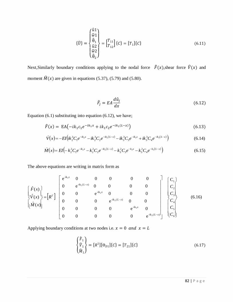
82 | P a g e

{ }

{

}

*

+ { } [ ]{ }

Next,Similarly boundary conditions applying to the nodal force ,shear force and

moment are given in equations (5.37), (5.79) and (5.80).

Equation (6.1) substituting into equation (6.12), we have;

(

)

(6.14) 3322

4

3

33

3

32

3

21

3

2

xLikxikxLikxikeCikeCikeCikeCikEIxV

(6.15) 3322

4

2

33

2

32

2

21

2

2

xLkxkxLikxikeCkeCkeCkeCkEIxM

The above equations are writing in matrix form as

(6.16)

C

e 0 0 0 0 0

0 e 0 0 0 0

0 0 e 0 0 0

0 0 0 e 0 0

0 0 0 0 e 0

0 0 0 0 0 e

)(ˆ

)(ˆ

)(ˆ

6

5

4

3

2

1

)(ik-

ik-

)(ik-

ik-

)(ik-

-ik

'1

3

3

2

2

1

1

C

C

C

C

C

R

xM

xV

xF

xL

x

xL

x

xL

x

Applying boundary conditions at two nodes i.e.

{

} [ ][ ]{ } [ ]{ }

83 | P a g e

{

} [ ][ ]{ } [ ]{ }

Combining equations (6.17) and (6.18), the nodal force vector can be written as

{ }

{

}

[

] { } [ ]{ }

Elimating { } from equations (6.11) and (6.19), the nodal displacement vector can be related to

the nodal force vector as

{ } [ ][ ] { }

{ } [ ]{ }

where, [ ] is the elemental dynamic stiffness matrix.

The above equation can be solved to obtain the nodal displacement vector { } for known nodal

forces.

{ } { }[ ]

{ } can be substituted into equation (6.11) to derive the constant { } as

{ } { }[ ]

After knowing constant { }, it can be substituted into equation (6.3) to obtain the at any

arbitrary points (XS) on the rod. i.e. putting

84 | P a g e

CHAPTER-7

7 RESULTS & DISCUSSION

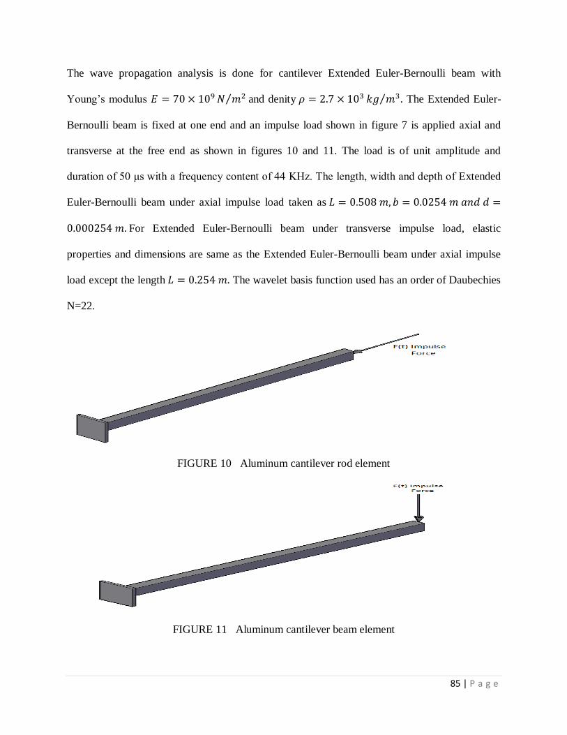
85 | P a g e

The wave propagation analysis is done for cantilever Extended Euler-Bernoulli beam with

Young‟s modulus ⁄ and denity ⁄ . The Extended Euler-

Bernoulli beam is fixed at one end and an impulse load shown in figure 7 is applied axial and

transverse at the free end as shown in figures 10 and 11. The load is of unit amplitude and

duration of 50 μs with a frequency content of 44 KHz. The length, width and depth of Extended

Euler-Bernoulli beam under axial impulse load taken as

For Extended Euler-Bernoulli beam under transverse impulse load, elastic

properties and dimensions are same as the Extended Euler-Bernoulli beam under axial impulse

load except the length The wavelet basis function used has an order of Daubechies

N=22.

FIGURE 10 Aluminum cantilever rod element

FIGURE 11 Aluminum cantilever beam element

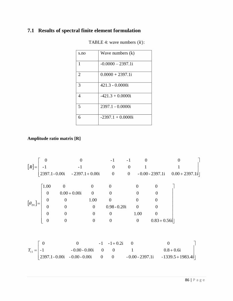
86 | P a g e

7.1 Results of spectral finite element formulation

TABLE 4: wave numbers :

s.no Wave numbers (k)

1 -0.0000 – 2397.1i

2 0.0000 + 2397.1i

3 421.3 - 0.0000i

4 -421.3 + 0.0000i

5 2397.1 - 0.0000i

6 -2397.1 + 0.0000i

Amplitude ratio matrix [R]

2397.1i0.00 2397.1i-0.00- 0 0 0.00i2397.1- 0.00i-2397.1

1 1 0 0 1- 1-

0 0 1- 1- 0 0

R

0.56i0.83 0 0 0 0 0

0 1.00 0 0 0 0

0 0 0.20i-0.98 0 0 0

0 0 0 1.00 0 0

0 0 0 0 0.00i0.00 0

0 0 0 0 0 00.1

D1

1983.4i1339.5- 2397.1i-0.00- 0 0 0.00i-0.00- 0.00i-2397.1

0.6i0.8 1 0 0 0.00i-0.00- 1-

0 0 0.2i1- 1- 0 0

11T

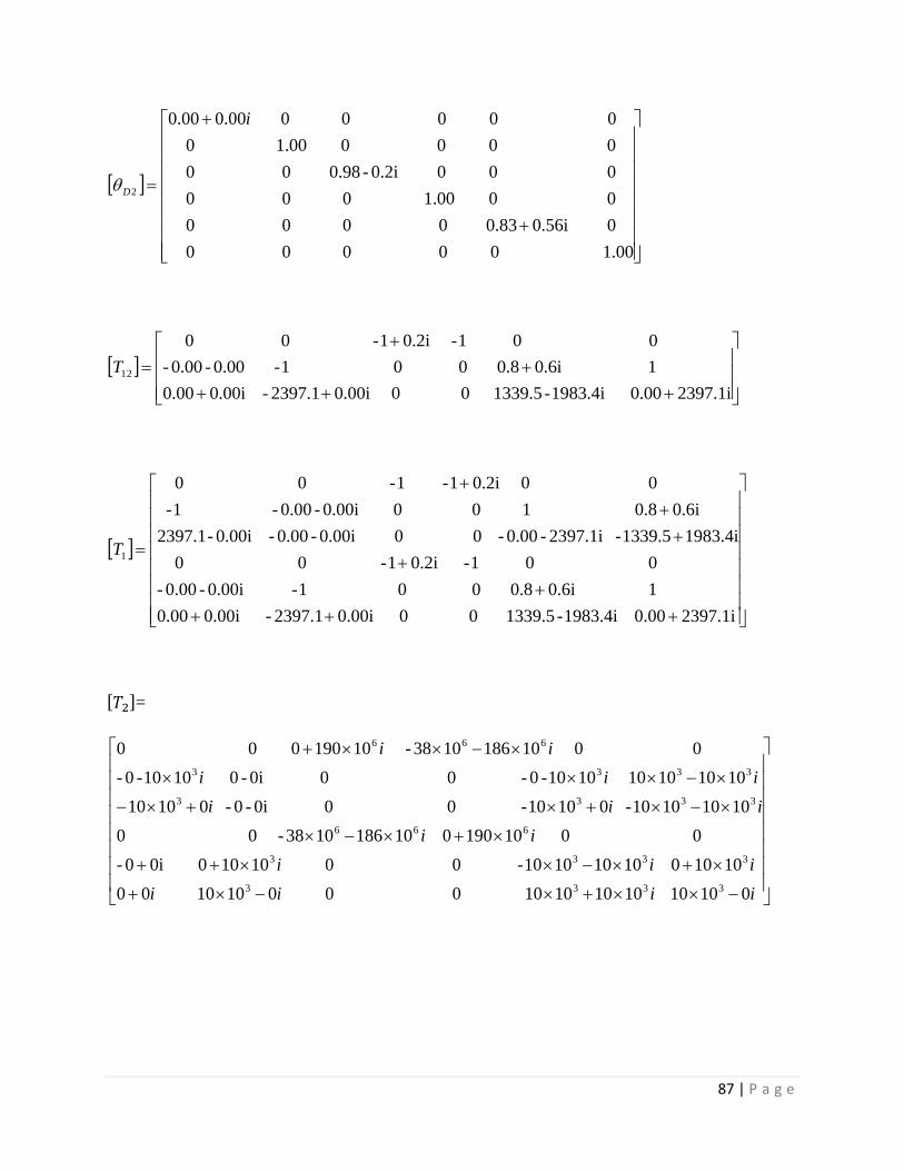
87 | P a g e

1.00 0 0 0 0 0

0 0.56i0.83 0 0 0 0

0 0 1.00 0 0 0

0 0 0 0.2i-0.98 0 0

0 0 0 0 1.00 0

0 0 0 0 0 00.000.0

2

i

D

2397.1i0.00 1983.4i-1339.5 0 0 0.00i2397.1- 0.00i0.00

1 0.6i0.8 0 0 1- 0.00-0.00-

0 0 1- 0.2i1- 0 0

12T

2397.1i0.00 1983.4i-1339.5 0 0 0.00i2397.1- 0.00i0.00

1 0.6i0.8 0 0 1- 0.00i-0.00-

0 0 1- 0.2i1- 0 0

1983.4i1339.5- 2397.1i-0.00- 0 0 0.00i-0.00- 0.00i-2397.1

0.6i0.8 1 0 0 0.00i-0.00- 1-

0 0 0.2i1- 1- 0 0

1T

[ ]=

iiii

iii

ii

iii

iii

ii

01010 10101010 0 0 01010 00

10100 10101010- 0 0 10100 0i0-

0 0 101900 101861038- 0 0

10101010- 01010- 0 0 0i-0- 01010

10101010 1010-0- 0 0 0i-0 1010-0-

0 0 101861038- 101900 0 0

3333

3333

666

3333

3333

666

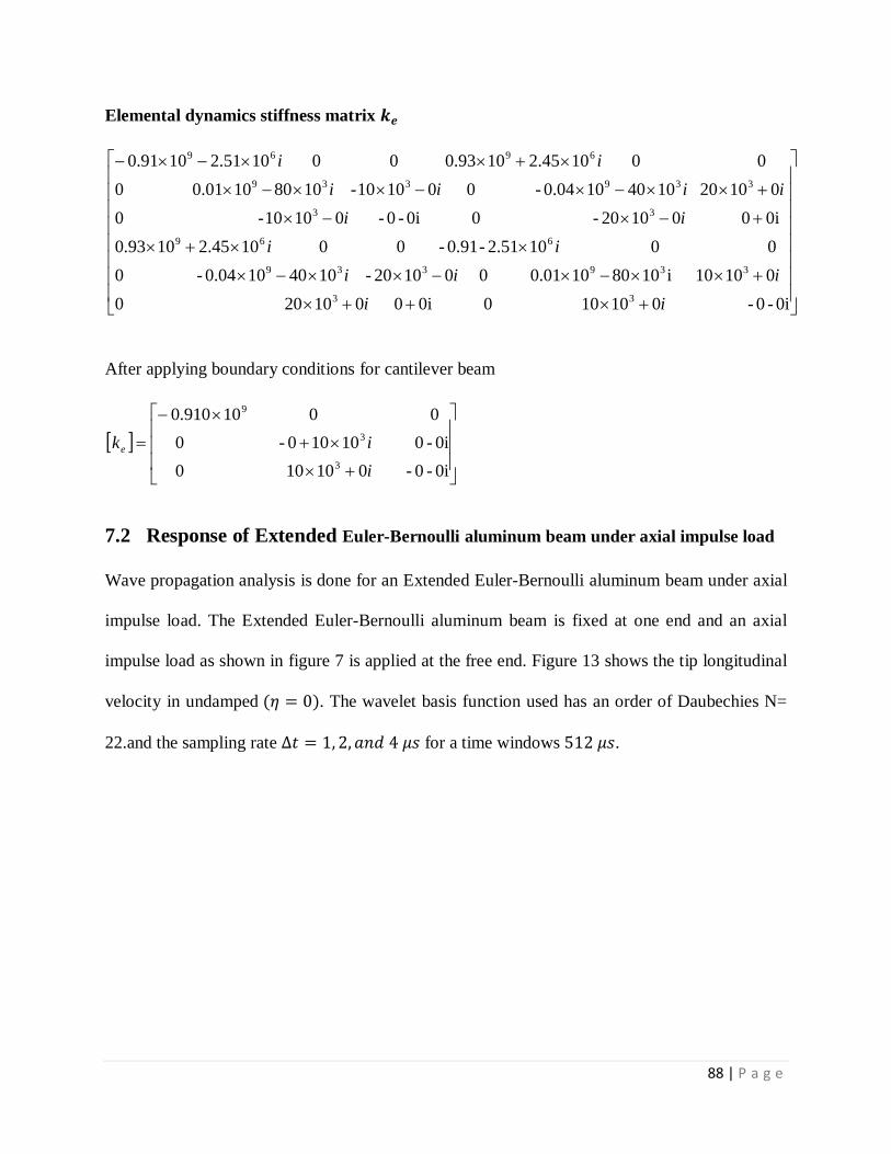
88 | P a g e

Elemental dynamics stiffness matrix

0i-0- 01010 0 0i0 01020 0

01010 i1080100.01 0 01020- 1040100.04- 0

0 0 102.51-0.91- 0 0 1045.2100.93

0i0 01020- 0 0i-0- 01010- 0

01020 1040100.04- 0 01010- 1080100.01 0

0 0 1045.2100.93 0 0 1051.21091.0

33

339339

669

33

339339

6969

ii

iii

ii

ii

iiii

ii

After applying boundary conditions for cantilever beam

0i-0- 01010 0

0i-0 10100- 0

0 0 10910.0

3

3

9

i

ike

7.2 Response of Extended Euler-Bernoulli aluminum beam under axial impulse load

Wave propagation analysis is done for an Extended Euler-Bernoulli aluminum beam under axial

impulse load. The Extended Euler-Bernoulli aluminum beam is fixed at one end and an axial

impulse load as shown in figure 7 is applied at the free end. Figure 13 shows the tip longitudinal

velocity in undamped . The wavelet basis function used has an order of Daubechies N=

22.and the sampling rate for a time windows .

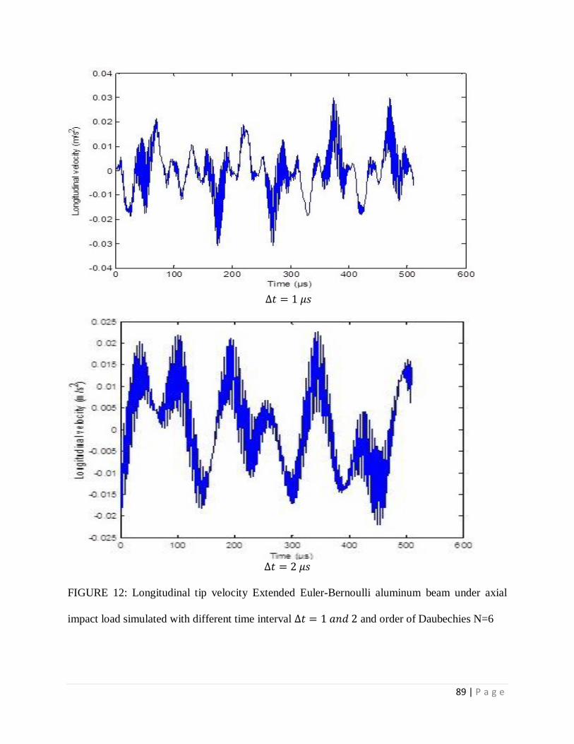
89 | P a g e

FIGURE 12: Longitudinal tip velocity Extended Euler-Bernoulli aluminum beam under axial

impact load simulated with different time interval and order of Daubechies N=6

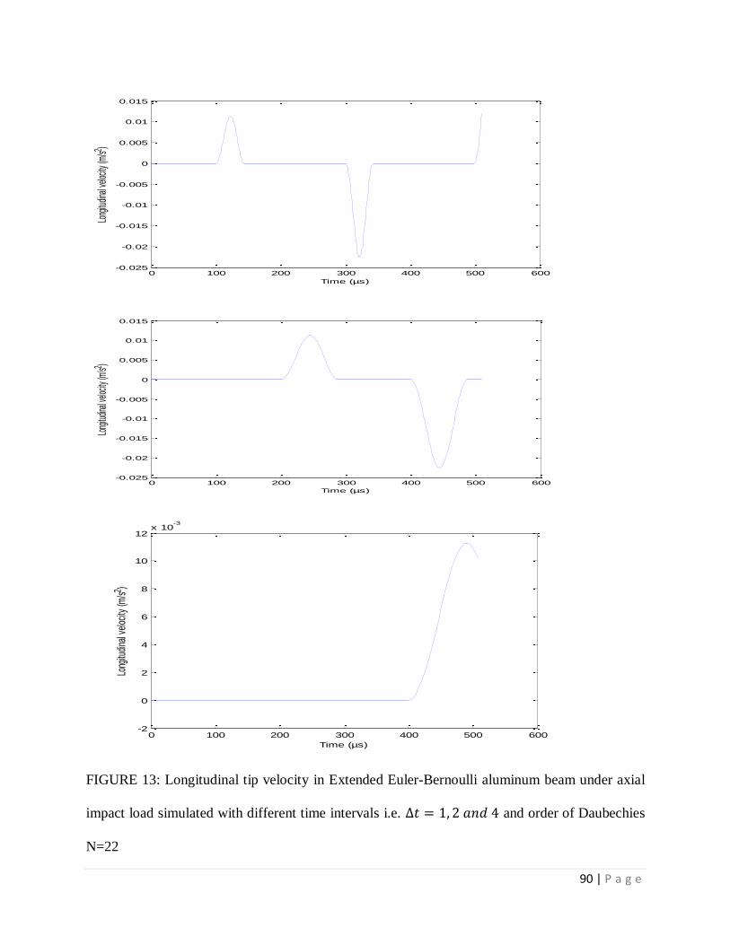
90 | P a g e

FIGURE 13: Longitudinal tip velocity in Extended Euler-Bernoulli aluminum beam under axial

impact load simulated with different time intervals i.e. and order of Daubechies

N=22

0 100 200 300 400 500 600-0.025

-0.02

-0.015

-0.01

-0.005

0

0.005

0.01

0.015

Time (µs)

Long

itudin

al ve

locity

(m/s2 )

0 100 200 300 400 500 600-0.025

-0.02

-0.015

-0.01

-0.005

0

0.005

0.01

0.015

Time (µs)

Long

itudin

al ve

locity

(m/s2 )

0 100 200 300 400 500 600-2

0

2

4

6

8

10

12x 10

-3

Time (µs)

Long

itudi

nal v

eloc

ity (m

/s2 )

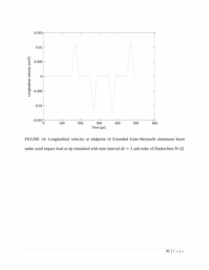
91 | P a g e

FIGURE 14: Longitudinal velocity at midpoint of Extended Euler-Bernoulli aluminum beam

under axial impact load at tip simulated with time interval and order of Daubechies N=22

0 100 200 300 400 500 600-0.015

-0.01

-0.005

0

0.005

0.01

0.015

Time (µs)

Longitudin

al velo

city (

m/s

2)

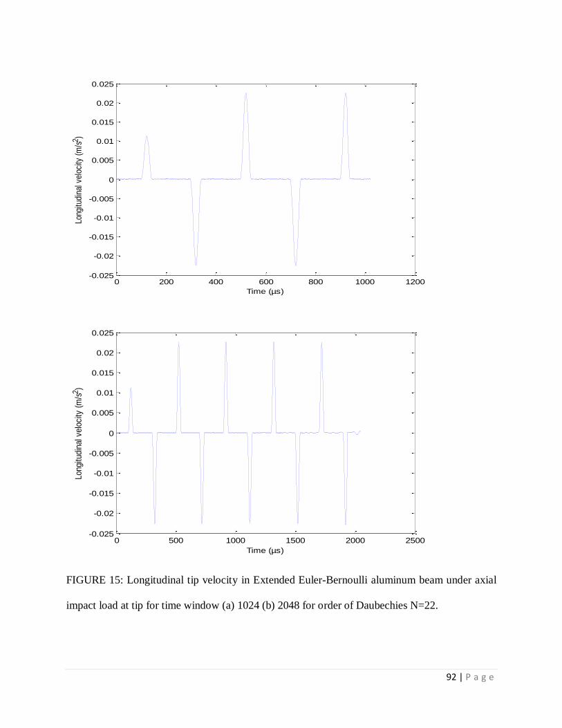
92 | P a g e

FIGURE 15: Longitudinal tip velocity in Extended Euler-Bernoulli aluminum beam under axial

impact load at tip for time window (a) 1024 (b) 2048 for order of Daubechies N=22.

0 200 400 600 800 1000 1200-0.025

-0.02

-0.015

-0.01

-0.005

0

0.005

0.01

0.015

0.02

0.025

Time (µs)

Long

itudi

nal v

eloc

ity (

m/s

2 )

0 500 1000 1500 2000 2500-0.025

-0.02

-0.015

-0.01

-0.005

0

0.005

0.01

0.015

0.02

0.025

Time (µs)

Long

itudi

nal v

eloc

ity (

m/s

2 )

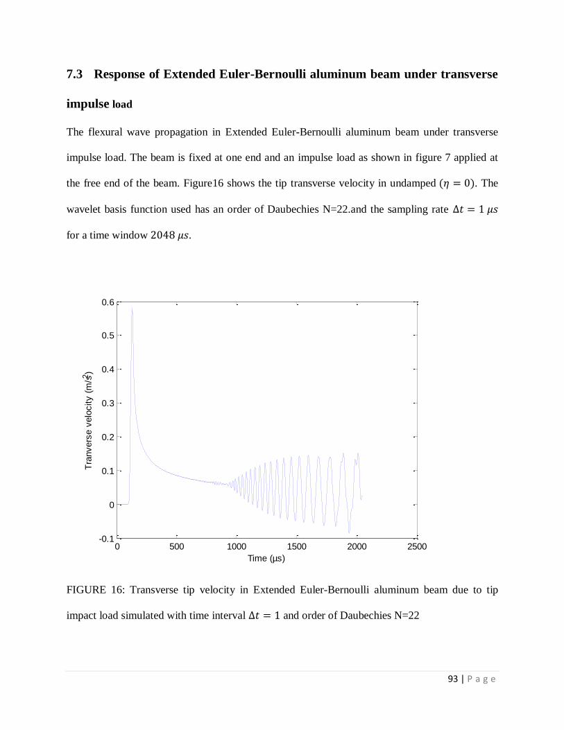
93 | P a g e

7.3 Response of Extended Euler-Bernoulli aluminum beam under transverse

impulse load

The flexural wave propagation in Extended Euler-Bernoulli aluminum beam under transverse

impulse load. The beam is fixed at one end and an impulse load as shown in figure 7 applied at

the free end of the beam. Figure16 shows the tip transverse velocity in undamped . The

wavelet basis function used has an order of Daubechies N=22.and the sampling rate

for a time window .

FIGURE 16: Transverse tip velocity in Extended Euler-Bernoulli aluminum beam due to tip

impact load simulated with time interval and order of Daubechies N=22

0 500 1000 1500 2000 2500-0.1

0

0.1

0.2

0.3

0.4

0.5

0.6

Time (µs)

Tra

nvers

e v

elo

city (

m/s

2)

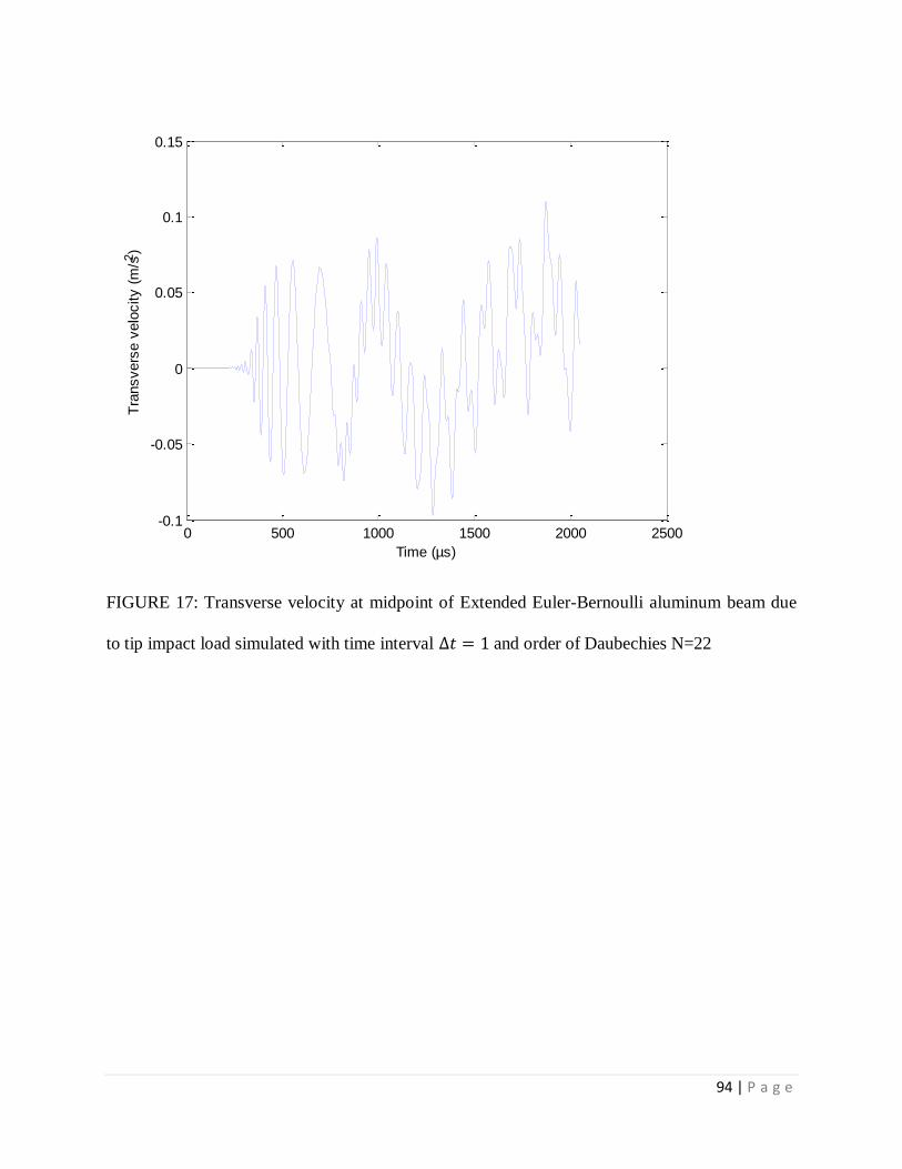
94 | P a g e

FIGURE 17: Transverse velocity at midpoint of Extended Euler-Bernoulli aluminum beam due

to tip impact load simulated with time interval and order of Daubechies N=22

0 500 1000 1500 2000 2500-0.1

-0.05

0

0.05

0.1

0.15

Time (µs)

Tra

nsvers

e v

elo

city (

m/s

2)

95 | P a g e

CHAPTER ~ 8

8 Conclusion

96 | P a g e

The formulation and validation of wavelet spectral element for simulation of wave propagation

in an Extended Euler-Bernoulli aluminum beam has been presented.

1 Spectral element method proves to be an efficient alternative to finite element analysis of

wave propagation problems and decreases the computational cost substantially.

2 The novelty of the spectral element developed is that it uses wavelet transform to reduce the

partial differential equations to ordinary differential equations unlike the solution which is used

in the spectral finite element formulation.

3 The finite element method analysis involves a large number of elements for the solution

whereas wavelet spectral finite element method involves only a single element for the solution.

4 When the time window is increased there is undulation in the axial velocities of the Extended

Euler-Bernoulli aluminum beam under axial impulse load.

5 When the time interval is increased i.e. when the number of sampling points is decreased the

solution has got more errors.

6 When the order of Daubechies increased the error in the solution decreased.

7 In case of Extended Euler-Bernoulli aluminum beam under axial impulse load, the velocity is

non-dispersive when as in case of beam under transverse impulse load it is dispersive.

97 | P a g e

References

98 | P a g e

[1] Amaratunga, K., Williams, J. R., Qian, S.and Weiss, J. Wavelet based Green‟s function

approach to 2D PDE‟s. Engineering Computation, 10 (4), 349–367, 1993.

[2] Amaratunga, K. and Williams, J. R. Time integration using wavelets. In: Proceedings of

SPIE, Wavelet Application for Dual Use, 2491, Orlando, FL, 894–902, 1995.

[3] Amaratunga, K. and Williams, J. R. Wavelet–Galerkin solution of boundary value

problems. Archives of Computational Methods in Engineering, 4 (3), 243–285, 1997.

[4] Beylkin, G. On the representation of operators in bases of compactly supported Wavelets.

SIAM Journal of Numerical Analysis., 6(6), 1716-1740, 1992.

[5] Bertoluzza, S. and Naldi, G. Some remarks on wavelet interpolation. Computational and

Applied Mathematics, 13(1), 13-32, 1994.

[6] Bathe, K. J. Finite element procedures. Prentice Hall, NJ, 1996.

[7] Beskos, D. E. Boundary element method in dynamics analysis part II (1986-1996). Applied

Mechanics Review, 50, 149-197, 1997.

[8] Batra, R. C. and Ching, H. K. Analysis of elasto dynamics deformations near a

crack/notch tip by the meshless local Petrov-Galerkin (MLPG) method. Computer Modeling in

Engineering and Science (CMES), 3(6), 717-730, 2002.

[9] Bajaba, N. S. and Alnefaie, K. A. Multiple damage detection in structures using wavelet

transforms. Emirates Journal for Engineering Research, 10 (1), 35-40, 2005.

[10] Canuto, C., Hussaini, M. Y., Quarteroni, A. and Zang, T. A. Spectral Method in Fluid

Dynamics, Springer Verleg, 1988.

99 | P a g e

[11] Cohen, A. Bi-orthogonal wavelets. Wavelets: A tutorial in theory and applications. C. K.

Chui, ed., Academic, San Diego, 123-152, 1992.

[12] Cohen, A., Daubechies, I. and Feauvean, J. C. Bi-orthogonal bases of compactly

Supported wavelets. Communications in Pure and Applied Mechanics, 45, 485-560, 1992.

[13] Daubechies, I. Orthonormal bases of compactly supported wavelets. Comm. In Pure and

Applied Mathematics, 41, 906-966, 1988.

[14] Donoho, D. L. Interpolating wavelet transforms. Technical Report, Department of

Statistics, Stanford University, 1992.

[15] Daubechies, I. Ten Lectures on Wavelets, SIAM, Philadelphia, 1992.

[16] Doyle, J. F. Wave propagation in structures. Springer, New York, 1999.

[17] Dahmen, W. Wavelet methods for PDEs some recent developments. Journal of

Computational and Applied Mathematics, 128(1–2), 133–185, 2001.

[18] Graff, K. F. Wave motions in elastic solids. Ohio State University Press, 1975.

[19] Grossmann, A. and Morlet, J. Decomposition of Hardy functions in to square Integrable

wavelets of constant shape. SIAM Journal of Mathematical Analysis, 15, 723-736, 1984.

[20] Glowinski, R., Lawton, W., Ravachol, M. and Tanenbaum, E. Wavelet solution of

linear and nonlinear elliptic, parabolic and hyperbolic problems in one space dimension. In:

Proceedings of the 9th International Conference on Numerical Methods in Applied Sciences and

Engineering, SIAM, Philadelphia, 1990.

100 | P a g e

[21] Graps, A. An Introduction to Wavelets. Computational Science and Engineering, 2(2),

1995.

[22] Gopalakrishnan, S., Chakraborty, A. and Mahapatra, D.Y. Spectral finite Element

method: Wave propagation, diagnostics and control in an-isotropic and In-homogeneous

structures. Springer, 2007.

[23] Gurley, K. and Kareem, A. Applications of Wavelet Transforms in Earthquake, Wind

and Ocean Engineering. Department of Civil Engineering and Geological Sciences, University

of Notre Dame, Notre Dame, IN, 46556

[24] Hu, F. Q., Hussaini, M. Y. and Rasetarinera, P. An analysis of the discontinuous

Galerkin method for wave propagation methods. Journal of Computational Physics, 151(2), 921-

946, 1999.

[25] Hong, T. K., Kennett, B. L. N. On a wavelet based method for the numerical simulation

of wave propagation. Journal of Computational Physics, 183, 577-622, 2002.

[26] Han, J. G., Ren, W. X. and Huang, Y. A spline wavelet finite-element method in

structural mechanics. International Journal for Numerical Methods in Engineering, 66,166–190,

2006.

[27] Hariharan, G. Solving finite length beam equation by the Haar wavelet method.

International Journal of Computer Applications, 9(1), 27-34, 2010.

[28] Jameson, L. On the wavelet based differentiation matrix. Journal of Scientific Computing,

8(3), 1993.

101 | P a g e

[29] Joly, P., Maday, Y. and Perrier, V. Towards a method for solving partial differential

equations by using wavelet packet bases. Computer Methods in Applied Mechanics and

Engineering, 116 (2), 193–202, 1994.

[30] Kaiser, G. A Friendly Guide to Wavelets, Birkhauser, Boston, 44-45, 1994.

[31] Kumar, B. V. R and Mehra, M. International Journals of Computational Methods, 2, 75–

97, 2005.

[32] Kozbial, T. Application of Daubechies wavelets approximation to plate bending. Proc

.Appl. Math. Mech, 6, 231–232, 2006.

[33] Khatam, H., Golafshani, A. A., Beheshti-Aval, S. B. and Noori, M. Harmonic class

loading for damage identification in beams using wavelet analysis. Structural Health

Monitoring, 6(1), 67-80, 2007.

[34] Lancaster, P. Lambda matrices and vibrating systems. Pergamon Press, 1966.

[35] Latto, A., Resnikoff, H.L. and Tanenbaum, E. The evaluation of connection Coefficients

of compactly supported wavelets. Cambridge-USA, 1999.

[36] Loutridis, S., Douk, E. and Trochidis, A. Crack identification in double-cracked beams

using wavelet analysis. Journal of Sound and Vibration, 277, 1025–1039, 2004.

[37] Law, S. S., Wu, S. Q. and Shi, Z. Y. Moving Load and Prestress Identification Using

Wavelet-Based Method. Journal of Applied Mechanics, 75, 2008.

102 | P a g e

[38] Lee, U. and Kwon, K. Spectral element modeling of the thermally induced vibration of an

axially moving plate. Journal of Achievements in Materials and Manufacturing Engineering,

26(1), 65-72, 2008.

[39] Morlet, J., Arens, G., Fourgeau, I. and Giard, D. Wave propagation and sampling

theory. Geophysics, 47, 203-236, 1982.

[40] Morlet, J. Sampling theory and wave propagation. In C. H. Chen (ed.), NATO ASI Series,

Issues in Acoustic Signal/Image Processing and Recognition, Springer, Berlin, 1, 233-261, 1983.

[41] Mansur, W. J. A time stepping technique to solve wave propagation problems using the

boundary element method. PhD thesis, Southampton University, 1983.

[42] Mallat, S. G. Multi-resolution approximation and wavelets. Preprint GRASP Lab.,

Department of Computer and Information Science. University of Pennsylvania, 1986.

[43] Meyer,Y. Principed‟ incertitude, bases hilbertiennes et albebresd‟ operateurs‟. Seminaire

Bourbaki, 662, 1987.

[44] Ma, J., Xue, J., Yang, S. and He, Z. A study of the construction and application of a

Daubechies wavelet-based beam element. Finite Elements in Analysis and Design, 39, 965–975,

2003.

[45] Morton, K. and Mayers, D. Numerical Solution of Partial Differential Equations,

Cambridge University Press, 2005.

[46] Mehra, M. and Kumar, B. V. R. Communications in Numerical Methods in Engineering,

21, 313–326, 2005.

103 | P a g e

[47] Mitra, M. and Gopalakrishnan, S. Spectrally formulated wavelet finite element for Wave

propagation and impact force identification in connected 1-D waveguides. International journal

of solids and structures, 42, 4695-4721, 2005.

[48] Mitra, M. and Gopalakrishnan, S. Extraction of wave characteristics from wavelet-

based spectral finite element formulation. Mechanical Systems and Signal Processing, 20, 2046–

2079, 2006.

[49] Mitra, M. and Gopalakrishnan, S. Wavelet Based 2-D Spectral Finite Element

Formulation for Wave Propagation Analysis in Isotropic Plates. CMES, 15(1), 49-67, 2006.

[50] Mitra, M. and Gopalakrishnan, S. Wavelet based spectral finite element modeling and

detection of de-lamination in composite beams. Proc. R. Soc A, 462, 1721–1740, 2006.

[51] Mira Mitra.and Gopalakrishan, S. Wavelet Methods For Dynamical Problems With

Application to Metallic, Composites, and Nano-Composites Structures.

[52] Mitra, M. and Gopalakrishnan, S. Vibrational characteristics of single-walled Carbon-

nanotube: Time and frequency domain analysis. Journal of Applied Physics, 101,114320, 2007.

[53] Mitra, M. and Gopalakrishnan, S. Wavelet spectral element for wave propagation

Studies in pressure loaded axis symmetric cylinders. Journal of mechanics of Materials and

Structures, 2(4), 753-772, 2007.

[54] Mitra, M., Gopalakrishnan, S., Ruzzene, M., Apetre, N. and Hanagud, S. Perturbation

technique for wave propagation analysis in a notched beam using wavelet spectral element

modeling. Journal of Mechanics of Materials and Structures. 3 (4), 2008.

104 | P a g e

[55] Mitra, M. and Gopalakrishnan, S. Wave propagation analysis in anisotropic plate using

wavelet spectral element approach. Journal of Applied Mechanics, 75, 014504, 2008.

[56] Mehra, M.AIP Conference Proceedings, 1146, 241–252, 2009.

[57] Mahmoud, M. and Taha, R. A Neural-Wavelet Technique for Damage Identification in

the ASCE Benchmark Structure Using Phase II Experimental Data. Hindawi Publishing

Corporation Advances in Civil Engineering, 2010.

[58] Mehra, M., Patel, N. and Kumar, R. Comparison between different numerical methods

for discretization of PDEs a short review. Indian Institute of Technology Delhi, HauzKhas, New

Delhi–110116, India.

[59] Narayanan, G. V. and Beskos, D. E. Use of dynamic influence coefficients in forced

vibration problems with the aid of fast Fourier transform. Computers and Structures, 9, 445-450,

1978.

[60] Press et al, W. Numerical Recipes in FORTRAN, Cambridge University Press, New York,

498-499, 1992.

[61] Park, S. H. and Tassoulas, J. L. A discontinuous Galerkin method for transient analysis

of wave propagation in unbounded domains. Computer Method in Applied Mechanics and

Engineering, 191(36), 3983-4011, 2002.

[62] Rucka, M. and Wilde, K. Application of continuous wavelet transform in vibration based

damage detection method for beams and plates. Journal of Sound and Vibration, 297, 536–550,

2006.

105 | P a g e

[63] Sneddon, I. Fourier transforms. McGraw Hill, New York, 1951.

[64] Stromberg, J. O. A modified Franklin system and higher order spline system on as

unconditional bases for hardy spaces. Conf.in Honour of A. Zgmund, Wadsworth Mathematics

Series, 2, 1982.

[65] Shorr, B. F. The wave finite element method. Springer, Berlin, 2004.

[66] Sonekar, P. and Mitra, M. A wavelet-based model of one-dimensional periodic structure

for wave-propagation analysis. Proc. R. Soc. A, 466, 263-281, 2010.

[67] Trefethen, L. N. Spectral Methods in MATLAB, SIAM, Philadelphia, PA, 2000.

[68] Vonesch, C.,Blu, T. and Unser, M. Generalized Daubechies Wavelet Families. IEEE

Transactions on Signal Processing, 55(9), 4415-4429, 2007.

[69] Vampa, V. and Maria T. Martin and Lilliam Alvarez Diaz. A Daubechies wavelet

beam element .Mechanics Computational, 26, 654-666, 2007.

[70] Williams, J. R. and Amaratunga, K.A discrete wavelet transform without edge effects

using wavelet extrapolation. Journal of Fourier Analysis and Applications, 3(4), 435-449, 1997.

[71] Xiang, J. W. and Liang, M. Multiple crack identification using frequency measurement.

World Academy of Science, Engineering and Technology, 76, 2011.

[72] Yaghin, M. A. L. and Hesari, M. A. Using wavelet analysis in crack detection at the arch

concrete dam under frequency analysis with FEM. World Applied Sciences, 3 (4), 691-704, 2008.

106 | P a g e

[73] Zhou, Y. H. and Zhou, J. A modified wavelet approximation of deflections for solving

PDEs of beams and square thin plates. Finite Elements in Analysis and Design, 44, 773– 783,

2008.