MALDI IMAGING MASS SPECTROMETRY FOR SMALL MOLECULE

QUANTITATION AND EVALUATION FOR MARKERS OF DRUG

RESPONSE IN GLIOMAS

By

Sara L. Frappier

Dissertation

Submitted to the Faculty of the

Graduate School of Vanderbilt University

in partial fulfillment of the requirements

for the degree of

DOCTOR OF PHILOSOPHY

In

Chemistry

May, 2011

Nashville, Tennessee

Approved:

Dr. Richard M. Caprioli

Dr. Michael K. Cooper

Dr. Brian O. Bachmann

Dr. Reid C. Thompson

ii

This work is dedicated to those that I call family.

I am nothing without each and every one of you.

“To change the world, Start with one step.” -Dave Matthews

iii

ACKNOWLEDGEMENTS

This work would not have been possible without the financial support of the

Vanderbilt University Chemistry Department, and the DOD Advanced Program in

Proteomics W81XWH-05-1-0179.

I would like to thank my mentor, Richard Caprioli, for all of his guidance, and

support throughout my graduate student career. I had somewhat of a unique path towards

the completion of my degree and your patience and understanding allowed me to realize

my potential and push through until the end. You have always encouraged me to look

ahead with determination and keep the fire inside alive. This is invaluable advice that I

will carry with me always in every aspect of life.

To each of my committee members, Michael Cooper, Brian Bachmann and Reid

Thompson, thank-you for all of your input and enthusiasm to help progress this project to

its successful completion. Each of you has provided me personal and professional

guidance that has taught me a great deal and given me an intense desire to continue

working in clinical research.

I must also acknowledge the many people I have had the pleasure of working with

throughout my studies at Vanderbilt University. Thank-you to all of the past and present

members of the Mass Spectrometry Research Center, you have not only been colleagues,

you have been friends. I will always be proud to say that I am a member of the “Caprioli

Crew” and the times we have shared together will not be forgotten.

To everyone that has become my family here in Nashville, words cannot express

how grateful I am that I have each and every one of you in my life; Lindsey Roark, Lori

iv

and Blake McConnell, Nick Culton, Amber Wright, JT Meeks, Ashley Schneider and

Lacey and Jacob Culton. Through the ups and downs that this journey has taken me on,

you have all been there by my side. You have been there to celebrate my victories or

hold my hand when things didn’t always work out. You have kept me grounded and

focused on what is truly important in this life.

To my true family, I am blessed to have you. Mamma and Daddy-O, you have

always been an inspiration to me. Your example has shown me what it means to live a

full and meaningful life; a life of honesty, dedication, love, hope, happiness and faith.

Your endless support has made me into the person that I am today and I will always

strive to make you proud. To my brothers, David and Rob, although distance separates

us, I know that you always have my back. The comfort of this has helped me more than

you could ever know. And to the rest of the army that is the Frappier family, only we can

understand what it truly means to be a “Frap” and the overwhelming care and support

that is provided from such a blessed and love-filled family. Thank-you to each and every

one of you.

v

TABLE OF CONTENTS

Page

DEDICATION ............................................................................................................... ii

ACKNOWLEDGEMENTS ........................................................................................... iii

LIST OF TABLES ...................................................................................................... viii

LIST OF FIGURES ........................................................................................................ ix

Chapter

I. BACKGROUND AND OBJECTIVES ..................................................................... 1

Background ........................................................................................................ 1

Drug Discovery and Development ................................................................. 1

Current Methods for Drug Quantitation ......................................................... 5

MALDI Imaging Mass Spectrometry............................................................. 8

Instrumentation and Experimental Process ........................................... 8

Applications of MALDI IMS ............................................................. 12

Primary Brain Tumors ................................................................................. 16

Biomarker Discovery .................................................................................. 17

Summary and Objectives .................................................................................. 19

II. DRUG QUANTITATION PROTOCOL DEVELOPMENT ................................... 22

Overview ........................................................................................................ 22

Introduction .................................................................................................... 23

Issues with Quantitation ............................................................................. 23

Importance of Internal Standards ................................................................ 25

Results ............................................................................................................ 26

Signal Depth............................................................................................... 26

Area Ablated Calculation ........................................................................... 28

Tissue Dimension Calculations ................................................................... 30

Acquisition Methods .................................................................................. 32

Limits of Detection and Calibration Curves ................................................ 33

Discussion ....................................................................................................... 36

Materials and Methods .................................................................................... 41

Materials .................................................................................................... 41

Animal Dosing Methods ............................................................................. 41

Signal Depth Methods ................................................................................ 41

vi

Area Ablation Calculation Methods ............................................................ 42

Tissue Dimension Calculation Methods ...................................................... 43

Limits of Detection and Calibration Curve Methods ................................... 45

Dosed Tissue Analysis ............................................................................... 46

Drug Quantitation Using LC-MS/MS ......................................................... 46

Acknowledgements ......................................................................................... 47

III. ANALYSIS OF IMATINIB TREATED GL26 MURINE

CELL XENOGRAFTS .......................................................................................... 48

Overview ........................................................................................................ 48

Introduction .................................................................................................... 48

PDGF in Gliomas ....................................................................................... 48

Imatinib ...................................................................................................... 50

Use of Animal Models................................................................................ 51

Results ............................................................................................................ 52

Animal Implantation and Drug Dosing ....................................................... 52

Drug Detection and Quantitation ................................................................ 53

Proteome Response Study .......................................................................... 62

Discussion ....................................................................................................... 72

Materials and Methods .................................................................................... 81

Materials .................................................................................................... 81

Cell Culturing ............................................................................................. 82

Tumor Implantation .................................................................................... 82

Drug Dosing ............................................................................................... 84

Tissue Preparation and MALDI Imaging .................................................... 85

Data Pre-Processing ................................................................................... 86

Protein Identification .................................................................................. 87

Drug Quantitation Using LC-MS/MS ......................................................... 88

Acknowledgements ......................................................................................... 89

IV. ANALYSIS OF CYCLOPAMINE TREATED DIRECT

HUMAN GLIOMA CELL IMPLANTED MOUSE XENOGRAFTS .................... 91

Overview ........................................................................................................ 91

Introduction .................................................................................................... 92

Sonic Hedgehog Pathway in Gliomas ......................................................... 92

Cyclopamine .............................................................................................. 93

Direct Human Cell Xenograft Animal Models ............................................ 93

Results ............................................................................................................ 94

Animal Implantation and Drug Dosing ....................................................... 94

Drug Detection and Quantitation ................................................................ 96

Responder versus Non-Responder Proteome Study................................... 101

Discussion ..................................................................................................... 110

Materials and Methods .................................................................................. 115

Materials .................................................................................................. 115

vii

Tissue Preparation and MALDI Imaging .................................................. 115

Data Processing ........................................................................................ 117

Statistical Analysis ................................................................................... 118

Drug Quantitation Using LC-MS/MS ....................................................... 119

V. CONCLUSIONS AND PERSPECTIVES ........................................................... 120

The Value of MALDI Imaging in Drug Discovery and Development ............ 120

Future Directions .......................................................................................... 122

Appendix

A. PROTOCOL: QUANTITATION OF SMALL MOLECULES

WITH MALDI IMS ............................................................................................ 126

B. SIGNIFICANT FEATURE CHANGES AS A RESULT

OF CYCLOPAMINE TREATMENT IN THE

X-312-HGA AND X-402-GBM XENOGRAFTS ............................................... 134

LITERATURE CITED .................................................................................................. 14

viii

LIST OF TABLES

Table Page

1. Comparison of OLZ concentration values calculated with both LC-MS/MS

and MALDI-IMS methods ....................................................................................... 40

2. IMAT/d8-IMAT signal ratios taken from standards spotted on tumor

and normal tissues within a mouse brain ................................................................. 56

3. Imatinib concentrations calculated by MALDI-IMS methods ................................... 60

4. Imatinib concentrations calculated by LC-MS/MS methods ..................................... 61

5. Statistically significant features affected by IMAT presence .................................... 70

6. Protein Identification for tumor implanted mouse brain treated with IMAT.............. 73

7. Comparison of cyclopamine concentrations calculated by both LC-MS/MS

and MALDI-IMS methods ....................................................................................... 99

8. Significant peak change statistics for the X-312-HGA and X-406-GBM

xenograft mice ....................................................................................................... 105

9. Protein Identifications for significant features in the X-312-HGA

xenografts (CYC responsive) ................................................................................. 109

ix

LIST OF FIGURES

Figure Page

1. Overview of the drug discovery and development process ......................................... 3

2. Cartoon schematic of a typical direct tissue imaging experiment ................................ 7

3. Structure of the common matrices used in MALDI MS analysis .............................. 10

4. MALDI images of Olanzapine and its major metabolites in whole

body rat tissues ....................................................................................................... 15

5. Human glioma tumors.............................................................................................. 17

6. Developmental phases and estimated timeline for the discovery and

validation of biomarkers ......................................................................................... 19

7. MALDI MS/MS instrument schematics ................................................................... 25

8. AUC of OLZ versus the number of laser shots ......................................................... 27

9. AUC of d4-OLZ versus the number of laser shots .................................................... 28

10. Laser burn patterns on a thin layer of DHB photographed at 10x magnification ...... 31

11. Effects of acquisition method on signal ratios detected from a dilution

series of OLZ spiked matrix with 2 µM of d4-OLZ ................................................. 33

12. SRM spectra of olanzapine acquired on a MALDI LTQ XL .................................... 35

13. Calibration curve for OLZ....................................................................................... 36

14. Comparison of MALDI IMS and LC-MS/MS quantitation methods

for olanzapine ......................................................................................................... 39

15. IMAT images taken on a MALDI-LTQ XL ............................................................ 55

16. Imatinib images for the acutely dosed mouse brain samples .................................... 57

17. Imatinib images for the chronically dosed mouse brain samples .............................. 57

18. Imatinib calibration curve obtained using MALDI IMS methods ............................ 59

19. Imatinib quantitation results in ng/g for the acutely dosed mice............................... 63

x

20. Imatinib quantitation results in ng/g for the chronically dosed mice ........................ 64

21. Workflow for extracting regions of spectra from an image data set ......................... 65

22. Example Interval Plots created in the MiniTab® software program ......................... 67

23. Average protein spectra overlay comparing the various dosing groups .................... 69

24. Visualization of tumor cell growth in mouse brain sections ..................................... 95

25. MALDI MS/MS spectra of cyclopamine taken on a MALDI LTQ XL .................... 96

26. Cyclopamine calibration curve constructed using MALDI IMS methods ................ 98

27. Images of cyclopamine distribution in dosed X-302-AG brain .............................. 101

28. Survival advantage graph for CYC treated xenograft mice .................................... 102

29. Anti-human nuclear stained X-312-HGA brain section showing the

Various brain regions selected for analysis ............................................................ 104

30. SAM results for the Invaded Striatum region of the dosed versus non-dosed

xenograft samples ................................................................................................. 107

31. Correlation of m/z features in biopsy and xenograft tissues ................................... 124

1

CHAPTER I

BACKGROUND AND OBJECTIVES

Background

Drug Discovery and Development

The driving force behind drug discovery and development is to connect the

process of understanding a disease with bringing a safe and effective new treatment to

patients. Scientists work to piece together the basic causes and biological intricacies of

disease at the level of genes, proteins and cells. Out of this knowledge “targets” emerge

which potential new drugs might be able to affect. Researchers work to validate these

targets, discover a potential drug to interact with the chosen target, submit the compound

through a series of clinical tests for safety and efficacy and gain approval so that the new

drug can get into the hands of doctors and patients. The discovery and development of

new medicines is a long, complicated process and takes an average of 10-15 years.1, 2

The

average cost to research and develop each successful drug is estimated to be $800 million

to $1 billion.3 This accounts for the thousands of failures that a company must go through

before successfully producing a viable drug compound. For every 5,000- 10,000

compounds that enter the research and development (R&D) pipeline, ultimately only one

receives approval. These numbers seem astronomical, but by developing a better

understanding of the R&D process which is outlined in Figure 1, one can see why so

many compounds don‟t make it through the process and why it takes immense resources,

2

the best scientific minds, highly sophisticated technology, interdisciplinary collaboration

and complex project management to get one successful drug to patients.

Before any potential new medicine can be investigated, scientists must be able to

understand the disease being treated. It is necessary to elucidate the underlying cause of

the condition as well as how the genes are altered, how that affects the proteins they

encode and how those proteins interact with each other in living cells. These changes

directly relate to how the disease affects the patient. This knowledge is the basis for

treating the problem and guides research for the discovery of new therapeutic

compounds. Researchers from government, academia and industry all contribute to this

knowledge base.4 However, even with new tools and insights, this research takes many

years of work and, too often, leads to frustrating dead ends. Thus, there is an ever present

need for new technologies and methods to assist in understanding the underlying cause of

a disease. Even if the research is successful, it will take many more years of work to turn

this basic understanding of what causes a disease into a new treatment.

Once there is enough understanding of a disease, pharmaceutical researchers

select a “target” for a potential new medicine. This “target” is usually a gene or protein

involved with the disease that can interact with a drug compound. It is then, that large

screening processes begin to look for a lead compound. Once a potential compound is

identified initial Absorption, Distribution, Metabolism, Excretion and Toxicological

(ADME/TOX) studies are performed. The pharmacokinetic and pharmacodynamic

(PK/PD) tests are performed both in-vitro and in-vivo in what are known as the pre-

clinical trials. The results for these analyses help scientists to understand what the drug

does, how it works, as well as any side effects or safety issues.5

3

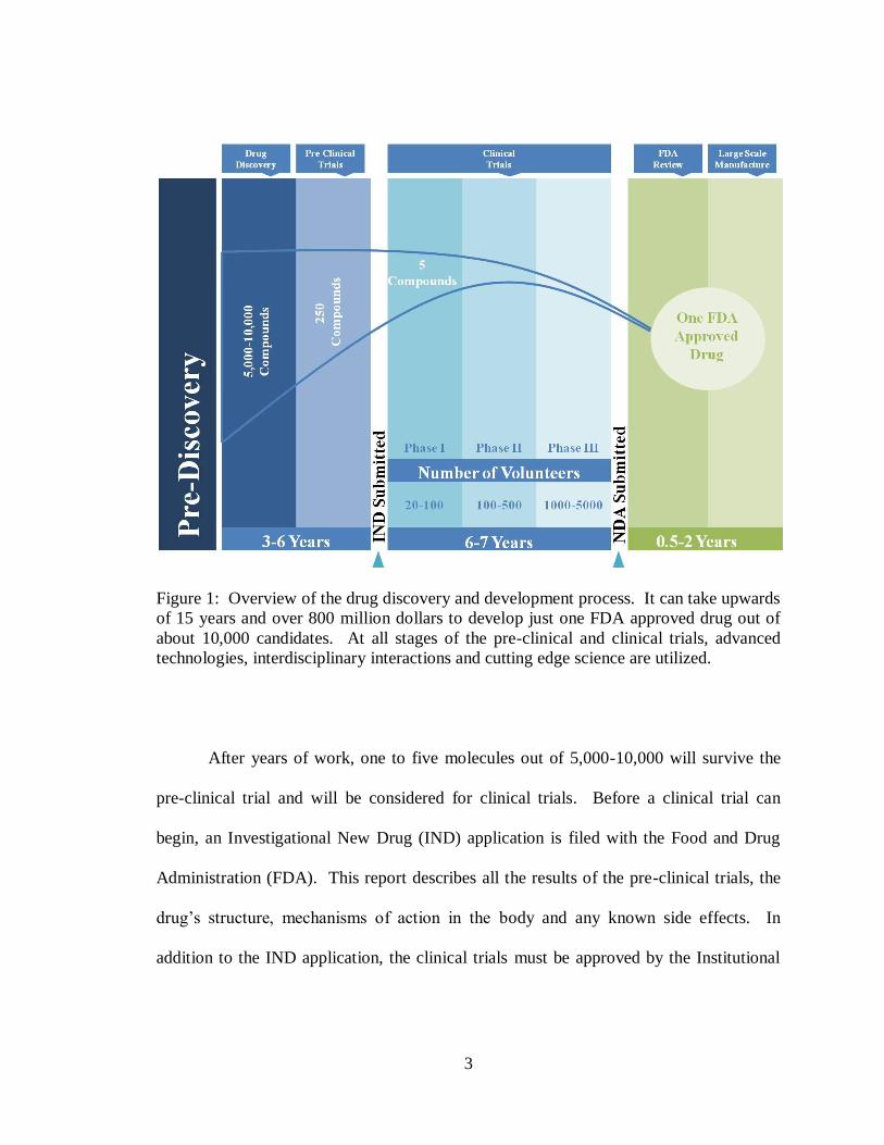
Figure 1: Overview of the drug discovery and development process. It can take upwards

of 15 years and over 800 million dollars to develop just one FDA approved drug out of

about 10,000 candidates. At all stages of the pre-clinical and clinical trials, advanced

technologies, interdisciplinary interactions and cutting edge science are utilized.

After years of work, one to five molecules out of 5,000-10,000 will survive the

pre-clinical trial and will be considered for clinical trials. Before a clinical trial can

begin, an Investigational New Drug (IND) application is filed with the Food and Drug

Administration (FDA). This report describes all the results of the pre-clinical trials, the

drug‟s structure, mechanisms of action in the body and any known side effects. In

addition to the IND application, the clinical trials must be approved by the Institutional

4

Review Board (IRB) and throughout the trials regular reports are monitored and

submitted to both the FDA and IRB. 6

The clinical trials consist of three phases. Phase I is a small initial test performed

in 20-100 healthy volunteers to see if the compound is safe for use in humans. The

ADME of the drug is studied as well as any side effects that result. Phase II trials focus

on testing the effectiveness of the compound on the indicated disease. The trial includes

100-500 patients and evaluates if the drug is targeting the disease as well as establishes

both dosing strength and dosing schedule. Phase III trials test a large group of patients to

show efficacy and safety. At hundreds of sites across the United States and worldwide,

1,000-5,000 patients are administered the drug and monitored. 3, 7

After clinical trials, a New Drug Application (NDA), which can be over 100,000

pages long, is filed with the FDA. The document contains all of the PK/PD results from

the trials. After approval the drug goes into manufacturing and distribution and ongoing

studies are maintained to continue monitoring the drug‟s performance.8

Throughout this long and complex process, one can identify numerous areas

where cutting edge technologies, new methods and interdisciplinary collaborations can

help to advance the understanding of human biology and disease. This can lead to

numerous breakthroughs for developing new medications. Researchers face great

challenges in understanding and applying these advances to the treatment of disease, but

these possibilities continue to grow as our scientific knowledge expands and becomes

increasingly more complete.

Mass Spectrometry (MS) has played a large role in these processes of developing

new drugs in all aspects of the drug development process. MS has been used to

5

characterize small molecule compounds, evaluate biomolecules for targets, protein

identification, analytical detection and quantitation. It has been used in all stages of pre-

clinical and clinical trials and there is room for growth of the technology‟s use in new and

innovative ways.

Current Methods for Drug Quantitation

Before modern day MS, small molecule quantitation was achieved using high

pressure liquid chromatography (HPLC) and ultraviolet (UV) detection. UV detectors

measure the ability of chromaphores in compounds within a sample to absorb UV light.

This can be accomplished at one or multiple wavelengths within the range or 190-400

nm. Most organic compounds can be measured by UV detectors.9 However, this

methodology suffered from lack of specificity and sensitivity. There are instances when

a drug metabolizes but the metabolites retention time and detection are the same as the

parent compound. Mass spectrometry has filled this need for both specificity and

sensitivity in the quantitation of small molecules along with the ability to distinguish

parent drug compound from its metabolites. Liquid chromatography tandem mass

spectrometry (LC-MS/MS) is now the de facto technique for providing quantitation data

for drug evaluation and submission for drug approval.10

The accepted way of performing MS quantitation is by using a mass spectrometer

capable of MS/MS fragmentation. MS/MS used in conjunction with quantitation is

commonly accomplished with a triple quadrupole or ion trap mass spectrometer. The

reason MS/MS is required is because many compounds have the same intact mass.

While many researchers use the first dimension of MS to perform quantitation, that

6

technique again suffers from lack of specificity especially in very complex matrices. The

second dimension of MS fragmentation in the majority of cases provides a unique

fragment. The combination of the specific parent mass and the unique fragment ion is

used to selectively monitor for the compound to be quantified. 11-14

However, while this

technique offers specificity and sensitivity the protocols required for the analysis cause

the loss of spatial information.

MALDI Imaging Mass Spectrometry

New advances in MS now provide the opportunity for investigative studies of

molecular interactions in intact tissue, much like studies conducted decades ago with

intact tissue for metabolic studies, but now with exquisite molecular specificity. In

particular, matrix-assisted laser desorption/ionization (MALDI) imaging mass

spectrometry (IMS) provides the investigator with the ability to analyze the spatial

distribution of molecules directly in tissue specimens.

IMS can be used to localize specific molecules such as drugs, lipids, peptides and

proteins directly from fresh frozen tissue sections with lateral image resolution down to

10 µm. Thin frozen sections (10-15 µm thick) are cut, thaw-mounted on target plates and

subsequently an energy absorbing matrix is applied. Areas are ablated with an UV laser,

typically having a target spot size of about 50 µm diameter, and give rise to ionic

molecular species that are recorded according to their mass-to-charge (m/z) values. Thus,

a single mass spectrum is acquired from each ablated spot in the array. Signal intensities

at specific m/z values can be exported from this array to give a two-dimensional ion

density map, or image, constructed from the specific coordinate location of that signal,

7

and its corresponding relative abundance. For high resolution images, matrix is deposited

in a homogeneous manner to the surface of the tissue in such a way as to minimize the

lateral dispersion of molecules of interest. This can be achieved by either automatically

printing arrays of small droplets or by robotically spraying a continuous coating. Each

micro spot or pixel coordinate is then automatically analyzed by MALDI MS (Figure 2).

From the analysis of a single section, images at virtually any molecular weight may be

obtained provided there is sufficient signal intensity to record.

Figure 2: Cartoon schematic of a typical direct tissue imaging experiment. The figure

demonstrates three types of matrix application; spray coating, high density droplet array,

and mist coating. Subsequent image acquisition is shown for each technique.

8

One of the most compelling aspects of IMS is the ability to simultaneously

visualize the spatial arrangement of hundreds of analytes directly from tissue without any

prior knowledge or need for target specific reagents such as antibodies. IMS provides the

ability to visualize post translational modifications and proteolytic processing while

retaining spatial localization. Other MS techniques, such as secondary ionization mass

spectrometry (SIMS), have also seen use for a variety of imaging applications.15-17

One

of the major advantages of SIMS is that it is capable of high resolution imaging (50-100

nm) for elements and small molecules (m/z <1000 Da). However, thus far, it has not

been shown to be effective for the analysis of proteins and large peptides.

Instrumentation and Experimental Process

The mass spectrometry instrumentation best suited for the analysis of peptides

and proteins directly from tissues is MALDI time-of-flight (TOF) technology. The

ablation process directed by the focused laser beam together with the high frequency of

the laser pulse renders this the favored ionization method for imaging. The duty cycle of

a modern TOF analyzer is an ideal match for the pulsed laser process and also has the

advantage of a theoretically unlimited mass range, high ion transmission efficiency,

multiplex detection capability and simplicity in instrument design and maintenance.18

A typical analysis of proteins directly from tissue is described for illustrative

purposes. Additional descriptions of a MALDI TOF MS can be found in other works. 19,

20 Two main experimental approaches may be used: profiling and imaging. Profiling

involves analyzing discrete areas of the tissue sections and subjecting the resulting

protein profiles to computational analysis. Typically, this uses 5–20 spots, each

9

approximately 0.2–1 mm in diameter. These experiments are designed to make

comparisons between representative areas on a single piece of tissue, such as normal

healthy area and diseased area, or between two different specimens. Thus, in the

„profiling‟ mode, fine spatial resolution is not required. A sufficient number of areas

must be sampled to gain statistical confidence in the results and this will vary depending

on the specific experiment. On the other hand, high resolution imaging of a tissue

requires that the entire tissue section is analyzed through an ordered array of spots, or

raster, in which spectra are acquired at intervals that define the image resolution (e.g.

every 50 μm in both the x and the y direction). 2D ion intensity maps, or images, can then

be created by plotting the intensities of any signal obtained as a function of its x, y

coordinates. The resulting images allow protein localization differences between and

among samples to be rapidly assessed.

Tissues used for analysis should be frozen in liquid nitrogen immediately after

resection to preserve the morphology and minimize protein degradation through

proteolysis. The tissue is usually sectioned in a cryostat to give 10-12 μm thick sections

and thaw-mounted onto an electrically conductive sample plate.19

Sample plates include

gold-coated or stainless steel metal plates and glass slides that have a conductive coating.

The tissue may be gently rinsed with ethanol as a fixative and wash to remove lipids and

salts. Alternatively, IMS compatible tissue staining protocols can be used in conjunction

with the optically transparent glass slides, allowing correlation of IMS data with

histological features of the same section by optical microscopy.21

MALDI IMS requires the application of energy absorbing matrix. This is

typically a small organic molecule that co-crystallizes with the analytes of interest on the

10

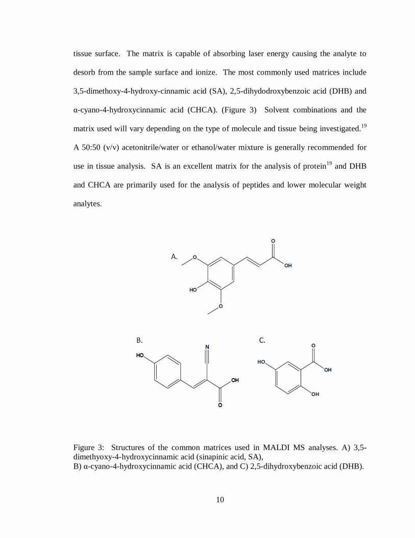
tissue surface. The matrix is capable of absorbing laser energy causing the analyte to

desorb from the sample surface and ionize. The most commonly used matrices include

3,5-dimethoxy-4-hydroxy-cinnamic acid (SA), 2,5-dihydodroxybenzoic acid (DHB) and

α-cyano-4-hydroxycinnamic acid (CHCA). (Figure 3) Solvent combinations and the

matrix used will vary depending on the type of molecule and tissue being investigated.19

A 50:50 (v/v) acetonitrile/water or ethanol/water mixture is generally recommended for

use in tissue analysis. SA is an excellent matrix for the analysis of protein19

and DHB

and CHCA are primarily used for the analysis of peptides and lower molecular weight

analytes.

Figure 3: Structures of the common matrices used in MALDI MS analyses. A) 3,5-

dimethyoxy-4-hydroxycinnamic acid (sinapinic acid, SA),

B) α-cyano-4-hydroxycinnamic acid (CHCA), and C) 2,5-dihydroxybenzoic acid (DHB).

11

For high resolution imaging, the matrix solution should be homogenously

deposited across the tissue section in such a manner to avoid significant lateral migration

of analytes. Currently, this is achieved by applying matrix solution to the tissue in either

a spotted array or a homogenous spray coating.19

A continuous and homogenous spray

coating allows the highest spatial resolution, but densely spotted arrays show higher

reproducibility and generally better spectra quality. A number of robotic spotting devices

are commercially available and utilize acoustic,22

piezoelectric,23

inkjet printer,24

and

capillary deposition techniques25

. Several robotic spray coating devices are also

commercially available and utilize a mist nebulizing method26

or a thermally-assisted

spray method.27

Protein analysis is usually performed on a linear TOF instrument to achieve

highest sensitivity. Ions formed and desorbed during the laser pulse are extracted and

accelerated into the field free region of the TOF analyzer. Ions are usually detected by a

multi-channel plate detector and the time of flight of the various ions is inversely

proportional to their m/z values. This time measurement is then converted to m/z through

appropriate calibration procedures. For the analysis of low molecular weight species, an

ion mirror or reflectron can be used in the ion flight path to compensate for the initial

velocity/energy distribution and improve resolution.28

Other analyzer combinations have been used with MALDI IMS including TOF-

TOF,23

orthogonal TOF and orthogonal Quadrapole-TOF (Q-TOF),29, 30

ion mobility,31

fourier transform ion cyclotron resonance (FTICR) 32, 33

and ion trap technologies.34, 35

These additional tools have provided capabilities for protein identification, high mass

12

resolution acquisition and the ability to detect small molecules such as drugs and

metabolites.23, 29-32, 34

Applications of MALDI IMS

To date, considerable effort has been focused on finding molecular markers as

early indicators of disease. MALDI IMS provides a means to visualize molecularly

specific information while maintaining spatial integrity. For example, cancer progression

is dependent on essential characteristics such as the presence of growth factors,

insensitivity to growth-inhibitory signals, evasion of apoptosis, high replicate potential,

sustained angiogenesis, and tissue invasion and metastasis.36

Alterations in protein

expression, proteolytic processing and post-translational modifications all contribute to

this cellular transformation. IMS analyses of tissue sections reflect the overall status of

the tissue, therefore, analyses of tissues in different states can reveal differences in the

expression of proteins which otherwise could not be predicted. Thus, IMS has been used

to image protein distributions in multiple types of cancer. Imaging analysis has been

used to probe proteome changes in mouse breast and brain tumor.37, 38

glioblastoma

biopsies,39

human lung metastasis to the brain,40

and prostate.37, 41

Identifying features

that display differential expression patterns between cancerous and normal tissue can

provide valuable insight into the molecular mechanisms, provide molecular diagnostic

and prognostic signatures, and identify possible drug targets in implicated pathways.

In addition to the ability to assist in disease differentiation/diagnosis, the

proteome signature of a tissue can also be used for determining the effects of drug/small

molecule administration to an animal model or patient. Over the past decade, proteins

13

have become principle targets for drug discovery and proteomics-oriented drug research

has come to the forefront of activity in this area. Proteomics can play a major role in drug

development including target identification, target validation, drug design, lead

optimization, and pre-clinical and clinical development.42

Due to the lengthy and

complex drug discovery process,43

it is essential to find ways to speed-up and streamline

this process. With the early assessment of the distribution of a drug candidate in targeted

tissues, IMS can greatly assist in the discovery and validation of processes related to drug

ADME.44, 45

For example, IMS can individually detect the presence and location of a

drug and its metabolites in a label-free protocol, a significant advantage over other small

molecule imaging techniques which typically require the addition of a radioactive tag to

the molecule of interest such as in autoradiography. Another advantage of IMS is that it

is capable of providing information on both the pharmacological and biological effects of

a drug in that it can detect molecular features that may be markers of drug efficacy or

toxicity. Other imaging techniques give little information on the molecular identity of

these biological endpoints. Thus, IMS can monitor the analyte of interest and also the

corresponding proteome response. An example of this is work performed in the

discovery of transthyretin as a marker for Gentamicin-induced nephrotoxicity in rat.46

Gentamicin-induced nephrotoxicity is seldom fatal and is usually reversible but often

results in long hospital stays. Thus, there is great interest for finding potential markers of

early toxicity and also to help elucidate the molecular mechanism. Investigators utilized

MALDI IMS to determine differential protein expression within the rat kidney (cortex,

medulla, and papilla), identified features of interest between dosed and control rat, and

then applied downstream protein identification procedures. Transthyretin was

14

significantly increased in the treated mouse kidney over control and these finding were

validated with western blot and immunohistrochemistry.46

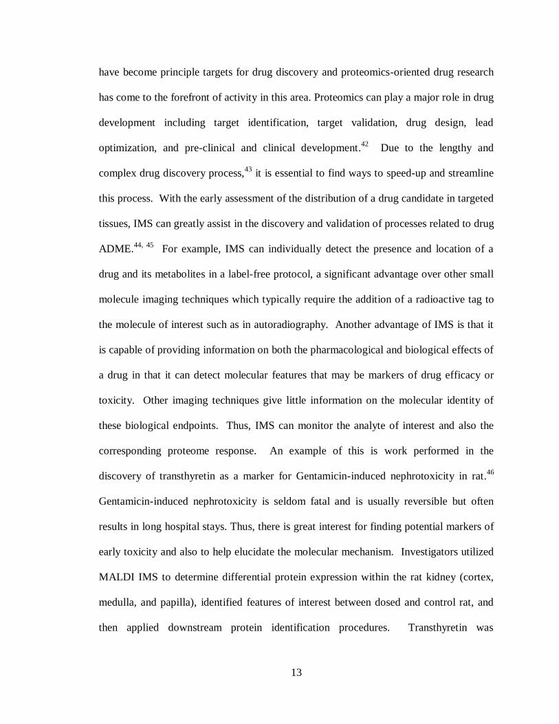
These same procedures can also be applied to whole-body animal tissue sections

for a system wide analysis in a single experiment.29

For whole-body sagittal tissue

sections, using the same sample preparation and analysis conditions described for IMS

experiments of tissues, exogenous small molecule signals found in various organs were

detected and used to produce images of dosed rat sections (Figure 4). By expanding the

capabilities of MALDI IMS to investigate multiple tissue types simultaneously across a

whole-body tissue section distinct protein patterns as well as small molecule distribution

can be identified and used to monitor whole-body system dynamics.

The molecular complexity of biological systems obviates the need for molecularly

specific tools to elucidate proteomic events in both spatial and temporal distributions.

One of the most effective ways to present such information is in the form of images, as

demonstrated through Magnetic Resonance Imaging (MRI), Positron Emission

Tomography (PET), and confocal microscopy. Similarly, images of the molecular

composition of living systems will allow us to gain a more comprehensive view of

biological processes and reveal complex molecular interactions. This approach will be

vital in elucidating molecular aspects of disease, such as primary brain tumors, and also

drug effectiveness by providing spatial and relevant time-based information.

15

Figure 4: MALDI images of Olanzapine and it major metabolites in whole body rat

tissues. A) Optical image of rat sagittal section across four gold MALDI target plates. B)

Ion image of Olanzapine MS/MS ion 256. C) Ion image of N-desmethyl metabolite

MS/MS ion 256. D) Ion image of 2-hydroxymethyl metabolite MS/MS ion 272. (Images

courtesy of Dr. Sheerin K. Shahidi)

16

Primary Brain Tumors

In this study the above technology will be applied to primary brain tumors.

Primary malignant brain tumors, which are tumors that start in the brain, account for 2

percent of all cancers in adults living in the United States (U.S.).47

There are many types

and subtypes of primary brain tumors. They include gliomas (which include

astrocytomas, oligodendrogliomas, and ependydomas), meningomas, medullablastomas,

pituitary adenomas, and central nervous system lymphomas.47, 48

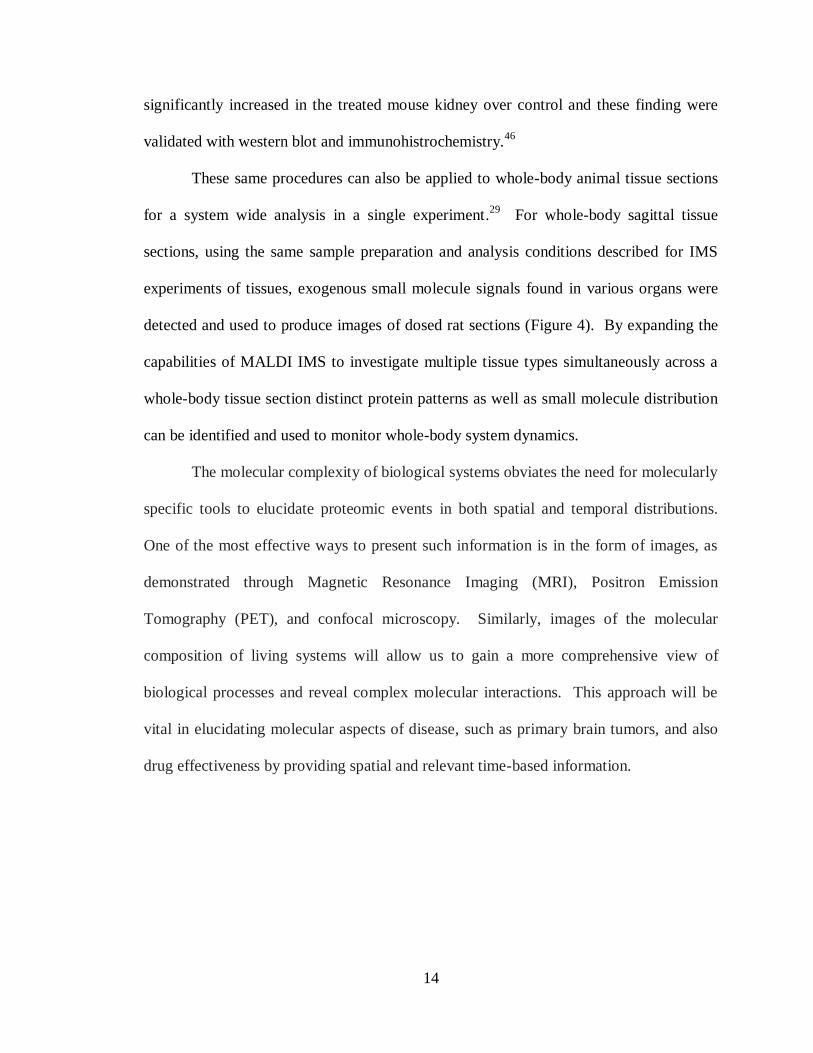
Figure 5A shows a

photograph of an excised patient brain with a glial tumor. The upper left portion of the

brain is consumed with the tumor mass. More recently the World Health Organization

(WHO) classification has been expanded to include additional types of primary tumors

such as angiocentric glioma, glialneuronal tumors, and atypical choroid plexus

papillomas.49

Brain tumors produce a variety of symptoms, including headache, seizure,

and neurological changes, whose onset could progress gradually or could occur at a very

rapid rate.

Diagnosis of brain tumors involves a neurological exam and various types of

imaging tests. Imaging techniques include MRI, computed tomography (CT), and PET

scan. Typically biopsies are performed as part of surgery to remove a tumor, but there are

cases where it is performed as a separate diagnostic procedure.47, 48

The standard

approach for treating brain tumors is to reduce the tumor as much as possible using

surgery, radiation treatment, or chemotherapy. Typically, such treatments are used in

various combinations with each other. Survival rates in primary brain tumors depend on

the type of tumor, patient age, functional status of the patient, and the extent of surgical

tumor removal. Figure 5B displays some typical glial tumor diagnoses along with the

17

average survival time for patients post surgery. In recent years, survival of the treatment

of a (solid) neoplasm of the brain has dramatically increased. Survival for the higher

graded tumors, as well as long term survival of younger patients, is also on the rise.

Patients with benign gliomas may survive for many years,50, 51

while survival in most

cases of glioblastoma multiforme is limited to a few months after diagnosis if treatment is

ignored. New molecularly targeted therapies are now coming to the forefront of research

with the hopes of increasing survival and quality of life for patients at even a much better

rate. Two of those therapies will be investigated in this study and are discussed in later

chapters.

Figure 5: Human glioma tumors. A) Photograph of an excised patient brain with a

glioma. B) The WHO naming classification for types of gliomas along with patient

survival post-surgery. The upper left portion of the brain is consumed with a tumor mass.

Biomarker Discovery

In recent years, clinical practice has shifted focus to the concepts of personalized

medicine which includes the use of targeted molecular therapy. Toward this goal,

biomarkers are providing early diagnosis of diseases and are helping physicians

18

determine safe and effective medication dosages as well as new possible drug targets.52

The National Institutes of Health (NIH) defined biomarkers as characteristics that are

objectively measured and evaluated as indicators of normal biological processes,

pathogenic processes, or pharmacologic responses to therapeutic interventions.53

In a

disease such as cancer the identification of a molecule or molecular signature that is

accurately indicative of these processes will be of extraordinary benefit to clinicians and

patients.54

For these biomarkers to be put into clinical practice for the goal of

personalized medicine, extensive research, testing and validation needs to be performed.

The main hypothesis driving the search for cancer biomarkers is the concept that

organs secrete a specific set of proteins representing a molecular signature indicative of

its physiological state.55

Genetic mutation and other altered biological processes will

affect the proteins that are secreted and expressed becoming a unique signature to a

disease phenotype.55

Detection and characterization of these molecular fingerprints

provides a unique view into the biology associated with various disease states. The

potential use of biomarkers for the early detection of cancer has compelled significant

research in this field.54, 56

Another advantage of biomarkers is the potential to aid clinicians in selecting

patients to undergo certain treatments. This research is conducted based on previous

evaluations of treatment efficacy and safety from patients exhibiting a specific biomarker

or group of markers. These markers may also be used to monitor response to treatment

and disease progression.57

Numerous studies have been published describing the discovery of putative

biomarkers using mass spectrometry. 25, 43, 58, 59

Although these studies established a

19

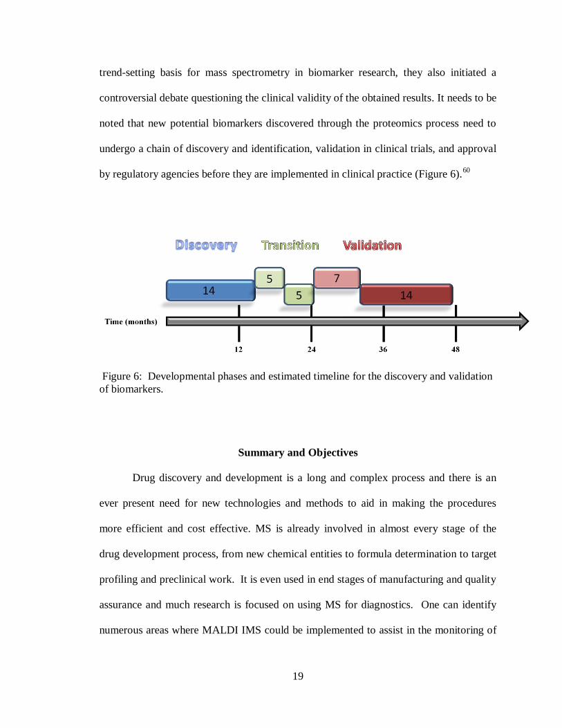
trend-setting basis for mass spectrometry in biomarker research, they also initiated a

controversial debate questioning the clinical validity of the obtained results. It needs to be

noted that new potential biomarkers discovered through the proteomics process need to

undergo a chain of discovery and identification, validation in clinical trials, and approval

by regulatory agencies before they are implemented in clinical practice (Figure 6).60

Figure 6: Developmental phases and estimated timeline for the discovery and validation

of biomarkers.

Summary and Objectives

Drug discovery and development is a long and complex process and there is an

ever present need for new technologies and methods to aid in making the procedures

more efficient and cost effective. MS is already involved in almost every stage of the

drug development process, from new chemical entities to formula determination to target

profiling and preclinical work. It is even used in end stages of manufacturing and quality

assurance and much research is focused on using MS for diagnostics. One can identify

numerous areas where MALDI IMS could be implemented to assist in the monitoring of

20

an administered drug and its metabolites, discover potential drug targets, assist in

diagnosis and evaluate the effects of a treatment.

The goal of the research presented here is to implement MALDI IMS for the

purpose of demonstrating its effectiveness and usefulness in the drug discovery and

validation processes. Drug distribution can be evaluated as well as quantitative

information obtained at localized points without losing spatial integrity due to

homogenization processes. Pharmacodynamic effects will also be studied toward

identifying possible features for biomarker validation that represent not only disease

state, but which can be used as indicators of targeted molecular therapy treatment

responses in glioma primary brain tumors.

Chapter II will address how with MALDI IMS it is possible to achieve small

molecule quantitation directly from tissue sections without the need for additional sample

treatment or separation techniques. Current methodologies do not have the capability of

retaining spatial information related to the drug concentration and require laborious

protocols involving homogenization and extraction techniques. The MALDI IMS

quantitation methodology developed will provide a solution to the issues presented by

LC-MS/MS methods. In addition, small molecule images will be obtained along with

protein images to allow for the correlation of drug tissue distribution and therapeutic

response within the same sample

The quantitation protocol has been applied to the investigation of two therapies

under investigation for the treatment of Glioblastomas (brain tumors of glial cell origin)

to determine the quantities of compound that reach the brain and tumor areas in mouse

models. In addition to drug quantitation, the treatment effects on the proteome of the

21

brain were investigated in relation to the amount of drug present. Chapter III focuses on

the investigation of the molecularly specific therapy imatinib and Chapter IV explores the

effects of the plant alkaloid cyclopamine on the gliomas. Future work will be discussed

in Chapter V that demonstrates how the affected protein signals found in the mouse

models can be related back to human tumor biopsies, demonstrating the feasibility of

utilizing mouse models to discover protein signatures that can be used as indicators of

therapy response. All of this work demonstrates the value that MALDI IMS has in the

drug development process and the advantages that it can provide.

22

CHAPTER II

DRUG QUANTITATION PROTOCOL DEVELOPMENT

Overview

Typically analysis of small molecules by MS has relied on the use of liquid

chromatography tandem mass spectrometry.11-14

Information ranging from structural

characterization to pharmacokinetic extraction studies can be obtained. These analytical

evaluations provide vital information regarding the preclinical ADME properties of

potential therapeutic compounds. In the pharmaceutical industry, distribution studies of

drug candidates are performed to gain knowledge about the localization and

accumulation of drugs in various tissues throughout an animal. While the LC-MS/MS

technique proved invaluable for drug quantities in tissues, there is a loss of spatial

information regarding drug distribution due to the necessity of homogenization

methodologies prior to analysis. MALDI mass spectrometry can fill this information gap

by providing drug distribution information with relatively easy sample preparation.

Typically in the past, MALDI MS has been overlooked as a viable option for small

molecule quantitative studies. Analysts have usually assumed that potential differences

in ionization efficiency between analyte and internal standards and an inherent

heterogeneity of the sample spot would limit MALDI MS as a quantitative technique.61

However, with the introduction of automated spotters and newly developed protocols, the

use of MALDI mass spectrometry for small organic molecule quantitation can become a

reproducible and reliable analytical procedure. The protocol developed here involving

23

robotic sample preparation combined with automated MALDI mass spectrometry

provides a viable method for quantitation of small molecules.

Introduction

Issues with Quantitation

LC-MS/MS quantitation for tissue samples, while effective, still faces many

issues that complicate the methodology. The first step of any quantitative tissue analysis

usually involves that the tissue must be homogenized which causes the loss of any spatial

information within the tissue. The next part of the process involves the extraction of the

small molecule to be analyzed using a series of centrifugation steps, solvent washes and

shaking, inversion or sonication. These processes can result in incomplete extraction,

loss of the compound due to sticking or leeching into tube walls of the equipment used or

ineffective sample transfer which would also affect the quantitation results. The LC

process could also create inconsistencies in the results. Shifts or convoluted retention

times due to changes in instrument parameters, interferences from other compounds and

loss of the small molecule due to sticking on the column are all issues that could create

fluctuations or inaccurate results. MALDI IMS can alleviate these issues while also

performing the analysis with minimal sample preparation steps and an analysis time on

the order of micro-seconds (µs) as opposed to minutes or even hours.

In the past, MALDI mass spectrometry was frequently not used for small

molecule analysis because of chemical interference from the MALDI matrix in the mass

range of a typical analysis (less than 1 kDa). However, the accepted way of performing

24

mass spectral quantitation is by using a mass spectrometer capable of MS/MS

fragmentation. MS/MS used in conjunction with quantitation is commonly accomplished

with a triple quadrupole or ion trap mass spectrometer. The reason MS/MS is required is

because many compounds have the same intact mass. Tandem mass spectrometry

involves analyzing the product ions of a particular precursor ion. In the MALDI MS/MS

instrument, the first mass analyzer acts as a mass filter by selectively allowing a narrow

mass window (0.2 Da to 5 Da depending on the instrument), usually centered on the

small molecule of interest, to continue on into the instrument, while preventing matrix

molecules from entering, helping to eliminate the matrix interference that has stifled

MALDI MS as a practical tool for small molecule analysis. The second process analyzes

the specific product ions of the molecules of interest which serves as a specific

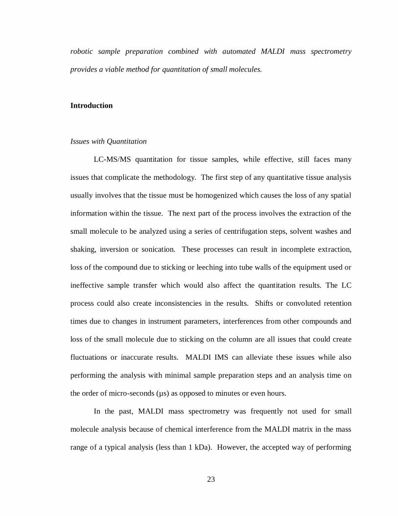
fingerprint. Figure 7 shows the schematics of both a Q-TOF and a LTQ, two instruments

used for MALDI MS/MS.

To assess changes in drug concentrations in a given tissue, pixel to pixel

reproducibility must be high, that is, two pixels close together having the same drug

concentrations should give the same spectra within acceptable standards. Although, this

will vary from experiment to experiment, typically variations of ±30% or less are deemed

acceptable. Factors that have a direct bearing on this aspect of the analysis include

ionization efficiency of a given molecule, ion suppression effects, extraction efficiency of

the matrix deposition process and the robustness and effectiveness of post acquisition

processing. High pixel to pixel reproducibility can be achieved by careful attention to

sample preparation and the matrix application steps. In addition, instrument parameters

such as voltage settings and laser power must be kept constant within a given experiment.

25

A robotic matrix application device is invaluable in removing operator to operator

variations.29

Figure 7: MALDI MS/MS instrument schematics. A) Schematic of the QStar XL (MDS

Sciex, Concord, Canada) equipped with an oMALDI source (20 Hz 337 nm nitrogen

laser) and a hybrid QqTOF mass analyzer B) Schematic of the MALDI LTQ XL

(Thermo Scientific Inc.)

Importance of Internal Standards

An internal standard (i.s.) should be used when performing MS quantitation. An

appropriate internal standard will control for extraction, sample introduction and

ionization variability. An internal standard should be added at the beginning of the

sample work-up and should be added at the same level in every sample including the

standards and should also give a reliable MS response. The amount of the internal

standard added needs to be well above the limit of detection but not so high as to

26

suppress the ionization of the analyte. The best internal standard is an isotopically

labeled version of the molecule you want to quantify. An isotopically labeled internal

standard will have a similar extraction recovery, ionization response, and separation

behavior as the analyte of interest.62

Results

Signal Depth

When acquiring small molecule data there a number of parameters that

must be considered in order to accurately represent the amount of drug that is in

the tissue. How many laser shots need to be acquired, how much of the matrix

spot needs to be sampled spatially and how should the internal standard and the

analyte desired be acquired from the same location. To begin investigating this,

Olanzapine (OLZ) dosed tissue sections were cut and spotted with DHB matrix in

50% methanol spiked with 2 µM of d4-OLZ internal standard. Various positions

across the matrix spots were analyzed collecting a spectrum every 45 laser shots.

The data was then plotted comparing the area under the curve (AUC) for the

MS/MS fragment (m/z 256) of the small molecule parent compound OLZ (m/z

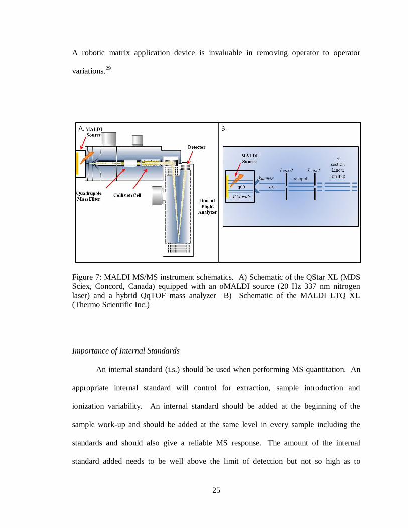
313) versus the number of laser shots. As can be seen in Figure 8, the majority of

the OLZ signal from the dosed tissue is acquired in the first 90 laser shots and

then tapers off quite drastically with most signal for each position being entirely

gone after 600 laser shots. Similarly, the d4-OLZ internal standard signal showed

27

Figure 8: Major OLZ fragment (m/z 256) area under the curve plotted against the

number of laser shots taken for each position across a DHB spot (approximately

250 µm diameter).

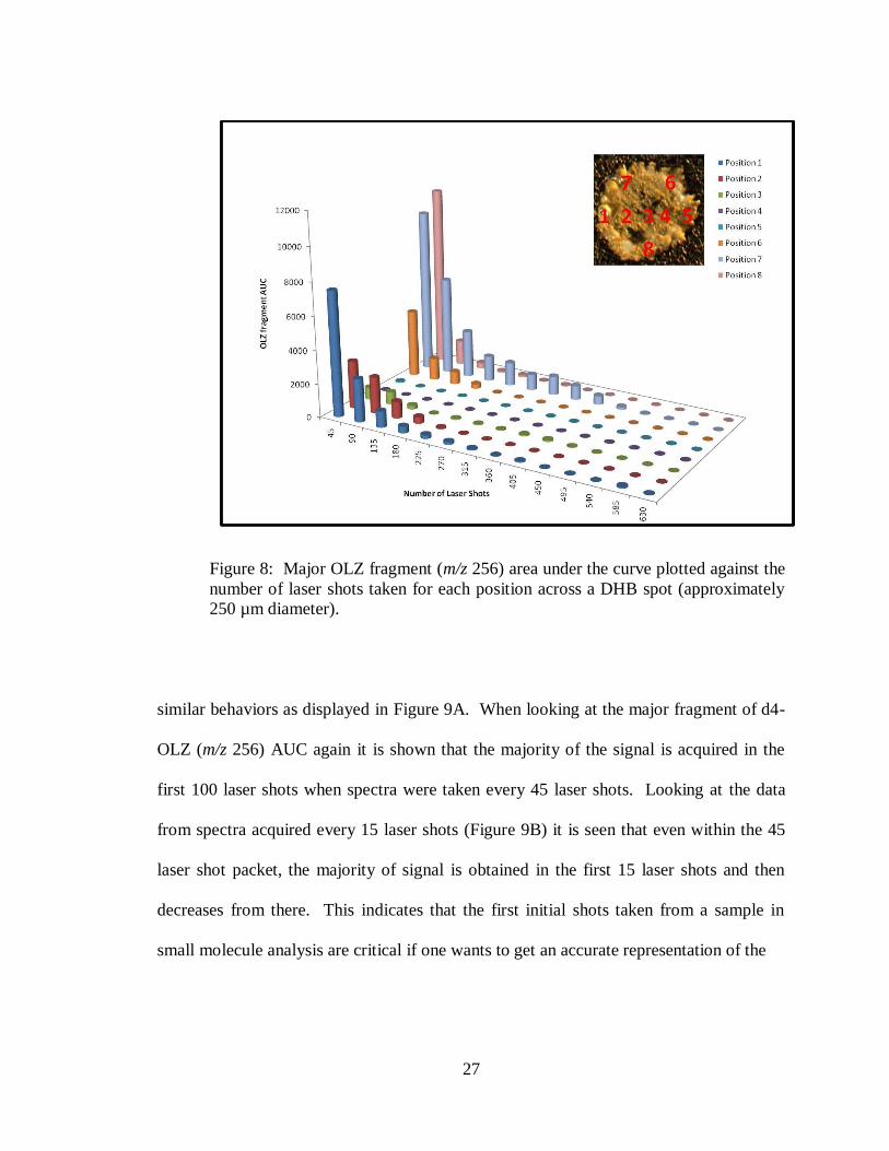
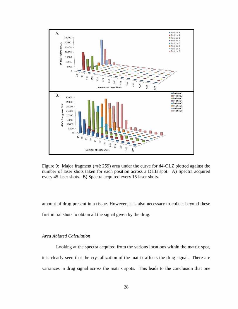
similar behaviors as displayed in Figure 9A. When looking at the major fragment of d4-

OLZ (m/z 256) AUC again it is shown that the majority of the signal is acquired in the

first 100 laser shots when spectra were taken every 45 laser shots. Looking at the data

from spectra acquired every 15 laser shots (Figure 9B) it is seen that even within the 45

laser shot packet, the majority of signal is obtained in the first 15 laser shots and then

decreases from there. This indicates that the first initial shots taken from a sample in

small molecule analysis are critical if one wants to get an accurate representation of the

28

Figure 9: Major fragment (m/z 259) area under the curve for d4-OLZ plotted against the

number of laser shots taken for each position across a DHB spot. A) Spectra acquired

every 45 laser shots. B) Spectra acquired every 15 laser shots.

amount of drug present in a tissue. However, it is also necessary to collect beyond these

first initial shots to obtain all the signal given by the drug.

Area Ablated Calculation

Looking at the spectra acquired from the various locations within the matrix spot,

it is clearly seen that the crystallization of the matrix affects the drug signal. There are

variances in drug signal across the matrix spots. This leads to the conclusion that one

29

position within the matrix spot is not an accurate representation of the amount of drug

present. It is necessary to evaluate multiple positions within a matrix spot. In order to

determine how many positions need to be analyzed to represent the amount of drug in a

given matrix spot, it must first be determined what area of the matrix spot is being

sampled by the laser. By evaluating laser burn patterns in a thin layer of DHB (sublimed

onto the target pate) the laser spot size dimensions can be determined. Laser spot size is

dependent on the number of laser shots being taken in a particular location and the laser

power used. For these experiments the laser power was kept constant at 20 µJ, which

was found to be the laser power necessary to obtain small molecule signal from the DHB

matrix spots. However, the number of laser shots taken at a particular location was

varied. The previous experiments showed that a bulk of signal was acquired in the first

90 laser shots, thus a burn pattern was achieved by shooting at a laser power of 20 µJ for

a total of 90 laser shots in the same spatial position (Figure 10A). This resulted in an

elliptical burn pattern size of 136 x 16 µm giving a total ablated area of 1709 µm 2

, while

a burn pattern achieved by shooting for a total of 600 laser shots, which is the number of

laser shots needed to ensure all the signal has been detected, was 153 x 31 µm giving a

total ablated area of 3725 µm2

(Figure 10B). Note that all laser burn pattern

measurements were taken from no less than a total of ten spots and resulted in percent

relative standard deviation (%RSD) values of less than 12%.

Looking at the laser burn areas from a micro-raster pattern it can be determined

what spatial resolution will be required to ablate all of the matrix in a given area. Laser

burn patterns were generated from a micro-raster of 50 µm x 4 positions within a spot

and an overall spatial array of 300 x 300 µm using both 90 laser shots per position and

30

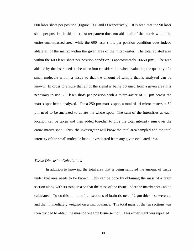
600 laser shots per position (Figure 10 C and D respectively). It is seen that the 90 laser

shots per position in this micro-raster pattern does not ablate all of the matrix within the

entire encompassed area, while the 600 laser shots per position condition does indeed

ablate all of the matrix within the given area of the micro-raster. The total ablated area

within the 600 laser shots per position condition is approximately 16650 µm2. The area

ablated by the laser needs to be taken into consideration when evaluating the quantity of a

small molecule within a tissue so that the amount of sample that is analyzed can be

known. In order to ensure that all of the signal is being obtained from a given area it is

necessary to use 600 laser shots per position with a micro-raster of 50 µm across the

matrix spot being analyzed. For a 250 µm matrix spot, a total of 14 micro-rasters at 50

µm need to be analyzed to ablate the whole spot. The sum of the intensities at each

location can be taken and then added together to give the total intensity sum over the

entire matrix spot. Thus, the investigator will know the total area sampled and the total

intensity of the small molecule being investigated from any given evaluated area.

Tissue Dimension Calculations

In addition to knowing the total area that is being sampled the amount of tissue

under that area needs to be known. This can be done by obtaining the mass of a brain

section along with its total area so that the mass of the tissue under the matrix spot can be

calculated. To do this, a total of ten sections of brain tissue at 12 µm thickness were cut

and then immediately weighed on a microbalance. The total mass of the ten sections was

then divided to obtain the mass of one thin tissue section. This experiment was repeated

31

Figure 10: Laser burn patterns on a thin layer of DHB photographed at 10x

magnification. All burn patterns were created with a laser power of 20µJ. A) 90 laser

shots per position in a 300 x 300 µm array. B) 600 laser shots per position in a 300 x 300

µm array. C) 90 laser shots per position in a 50 µm micro-raster pattern (x4) in a 300 x

300 µm array. D) 600 laser shots per position in a 50 µm micro-raster pattern (x4) in a

300 x 300 µm array.

five times for each tissue type analyzed. A 12 µm rat brain section had an average mass

of 1.02 mg with a RSD of 8%. To get the total tissue area, 12 µm brain sections were

cut, thaw mounted onto microscope slides, stained with cresyl violet and then scanned on

32

a flat bed scanner at 3200 dpi. The scanned images were imported into Adobe Photoshop

so that the area could be calculated. The area of the rat brain section was 250 mm2 with a

RSD of 0.3%. Using these dimensional measurements it is possible to calculate the

amount of tissue being sampled under any one given matrix spot.

Acquisition Methods

When using an internal standard it is important to evaluate the best way to acquire

both signal for the analyte of interest to be quantified and the signal given by the internal

standard to be used for normalization. Ideally, both signals will be acquired from the

same spatial location within the tissue section to give the most accurate results. As can

be seen by the signal depth experiments, the first shots of an acquisition are critical to

obtain all of the drug signal within a location. When alternating acquisition of analyte of

interest and internal standard this needs to be taken into consideration. Thus matrix spots

with known concentrations of OLZ standard and d4-OLZ standard were analyzed using

two methods. One method acquired internal standard (d4-OLZ) in the first 15 laser shots

and then the analyte of interest (OLZ) in the next 15 laser shots alternating from there

until 600 laser shots had been acquired at each location. The second method acquired

OLZ spectra for the first 15 laser shots and then d4-OLZ spectra in the next 15 laser shots

alternating until 600 laser shots had been acquired at each location. For each spot the

total intensity sum was calculated for the OLZ and d4-OLZ standards and then the ratio

of analyte/internal standard was calculated. Figure 11 shows the ratio results for the

matrix spots revealing that there is no significant difference between the two acquisition

33

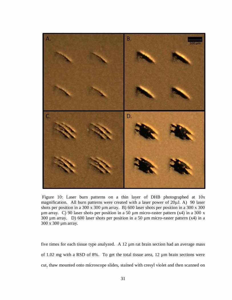
Figure 11: Effects of acquisition method on signal ratios detected from a dilution series

of OLZ spiked matrix with 2 µM of d4-OLZ. The OLZ first series indicates that the first

15 laser shots were acquired for the OLZ major fragment then the next 15 laser shots

were acquired for d4-OLZ major fragment, alternating until 600 laser shots were

acquired. The d4-OLZ first series is d4-OLZ for the first 15 laser shots and then OLZ,

alternating. The ratios collected by either method show no significant difference from

each other.

methods. The ratios fit within the standard deviations of both acquisition methods and

the percent difference was no higher than 15%.

Limits of Detection and Calibration Curves

The limit of detection (LOD) is usually defined as the lowest quantity or

concentration of a component that can be reliably detected with a given analytical

method. Intuitively, the LOD would be the lowest concentration obtained from the

34

measurement of a sample (containing the component) that would be able to be

discriminated from the concentration obtained from the measurement of a blank sample

(a sample not containing the component).63

64

The parameters used here to determine the

LOD are 3 standard deviations above the blank standard value.

A calibration curve is a method for determining the concentration of a substance

in an unknown sample by comparing the unknown to a set of standard samples of known

concentration. It is a plot of how the analyte signal changes with the concentration of the

analyte. A line or curve is fit to the data and the resulting equation is used to convert

readings of the unknown sample into concentration. In the instance of a linear fit :

Signal= slope x concentration + intercept

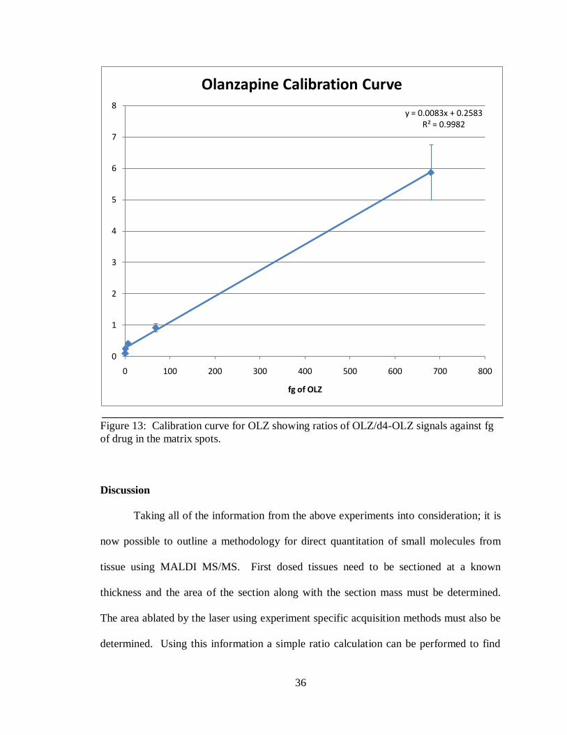
Calibration curve standards of OLZ were added to matrix solutions to yield final

concentrations of 100, 10, 1, and 0.1 ng/ml. A 2 µM concentration of d4-OLZ was also

added to the matrix as an internal standard in each solution. For the analysis of OLZ,

DHB in 50% methanol (MeOH) was used as the matrix. Using the Portrait™ 630, matrix

spots were deposited onto tissue sections in known volumes. Knowing the volume of

matrix standard deposited it is possible to calculate the amount of drug compound that

was deposited onto the tissue within the matrix spot. For the standard curve the amount

of drug within the matrix spots was 680, 68, 6.8 and 0.68 fg and a blank standard

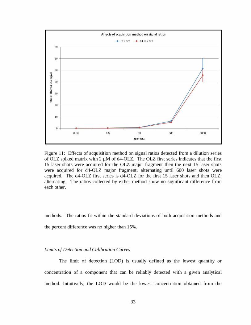
containing matrix only. As can be seen in Figure 12, the top panel shows a spectra taken

from a blank matrix spot and shows no signal at m/z 256 where the OLZ MS/MS

fragment would be, indicated by the red arrow. The bottom panel is a spectra taken from

a matrix spot containing 680 fg of OLZ and shows a clear signal at m/z 256.

35

Figure 12: SRM spectra of olanzapine acquired on a MALDI LTQ A) Spectra taken from

a matrix spot with no OLZ spike B) Spectra taken from a matrix spot containing 680 fg

OLZ.

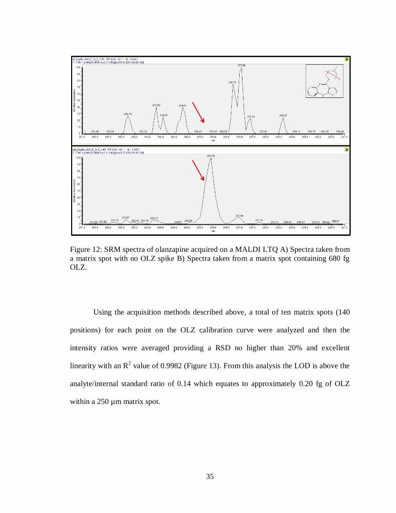
Using the acquisition methods described above, a total of ten matrix spots (140

positions) for each point on the OLZ calibration curve were analyzed and then the

intensity ratios were averaged providing a RSD no higher than 20% and excellent

linearity with an R2 value of 0.9982 (Figure 13). From this analysis the LOD is above the

analyte/internal standard ratio of 0.14 which equates to approximately 0.20 fg of OLZ

within a 250 µm matrix spot.

36

Figure 13: Calibration curve for OLZ showing ratios of OLZ/d4-OLZ signals against fg

of drug in the matrix spots.

Discussion

Taking all of the information from the above experiments into consideration; it is

now possible to outline a methodology for direct quantitation of small molecules from

tissue using MALDI MS/MS. First dosed tissues need to be sectioned at a known

thickness and the area of the section along with the section mass must be determined.

The area ablated by the laser using experiment specific acquisition methods must also be

determined. Using this information a simple ratio calculation can be performed to find

y = 0.0083x + 0.2583R² = 0.9982

0

1

2

3

4

5

6

7

8

0 100 200 300 400 500 600 700 800

fg of OLZ

Olanzapine Calibration Curve

37

the amount of tissue that is sampled within a specific location. For OLZ dosed rat brain

the tissue section area was found to be 250 mm2 and the tissue section mass was found to

be 1.02 mg. The area sampled by the laser in one position acquiring a total of 600 laser

shots at a laser power of 20 µJ is approximately 0.0035 mm2. To find the amount of

tissue sampled under one laser position the following equation was used: 250mm2/1.02

mg = 0.0035 mm2/X mg. From this calculation it was determined that 1.42x10

-5 mg of

tissue was sampled. A similar calculation was performed to determine the amount of

tissue sampled under a 250 µm matrix spot. The matrix spot has an area of 49087 µm2

which results in 5 x 10-4

mg of tissue sampled.

A calibration curve for the small molecule of interest must be acquired to provide

an equation for determining how much of the small molecule substance is in the sample

by comparing the unknown to a set of standard samples of known amounts. The dosed

tissue sections were then cut at 12 µm and spotted with matrix (DHB, 40 mg/ml in 50%

MeOH) spiked with an internal standard (d4-OLZ) and analyzed on the MALDI LTQ.

For each matrix spot a total of 14 locations were analyzed to completely ablate all of the

small molecule signal, taking 600 laser shots per location. A total of ten matrix spots

were analyzed for each dosed tissue. Using in-house software (developed by Surendra

Dasari) the total intensity sums were calculated for the OLZ signal and the d4-OLZ signal

at each location. These totals were then used to get the ratio of OLZ signal over d4-OLZ

signal within a matrix spot. The ratio values were plugged into the calibration curve‟s

linear equation to result in the amount of drug present in each spot. Dosed tissue sections

collected 2 hour (2h), 6 hour (6h) and 12 hour (12h) after a single dose of OLZ were

analyzed and resulted in an average of 790 fg, 70 fg, and 15 fg respectively of OLZ

38

compound. Dividing these values by the mass of the area sampled gave the average OLZ

concentration taken from the analyzed matrix spots for each of the dosed tissues with an

average RSD of 33%. At 2h post dose the OLZ concentration was 55.65 ng/mg, 6h post

dose was 4.89 ng/mg and 12h post dose was 1.84 ng/mg.

To compare the OLZ concentration results, an LC-MS/MS extraction protocol

was performed. The dosed tissues were homogenized, extracted and then analyzed on an

ESI TSQ Quantum triple-quadrupole system. Using this methodology for the 2h, 6h, and

12h samples, the concentrations of OLZ were found to be 57.30 ng/mg, 3.74 ng/mg and

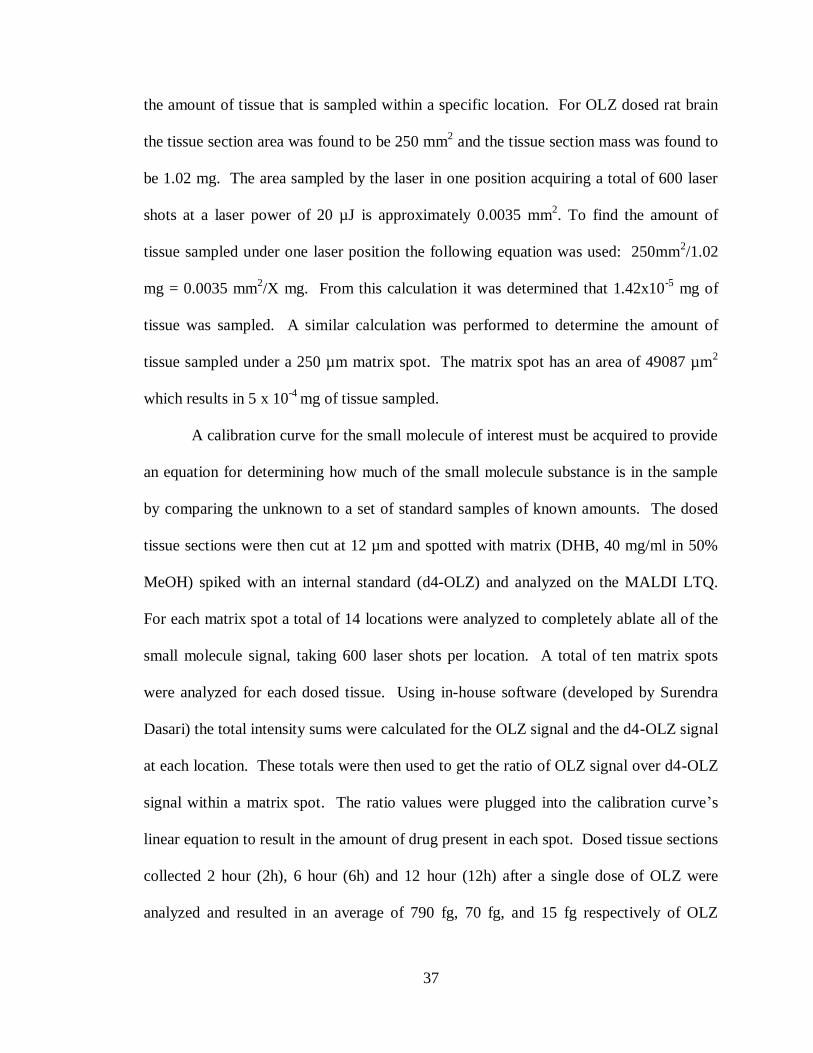
2.64 ng/mg respectively with an average RSD of 33%. Figure 14 displays the results for

both the MALDI MS/MS analysis and the LC MS/MS analysis. It can be seen that the

methodologies result in very similar concentrations for each of the dosed tissues. The 2h

sample has a percent difference of 3, the 6h sample has a percent difference of 24 and the

12h sample has a percent difference of 13 (Table 1). This demonstrates that the MALDI

MS/MS methodology developed here can be used to provide an accurate drug

quantitation for dosed tissue sections with excellent reproducibility and low standard

deviations.

In addition to the experiment descriptions provided in the material and methods

section of this chapter a detailed step by step protocol is included in Appendix A that

outlines the methodology developed to obtain absolute drug concentration directly from

tissue sections using MALDI IMS.

39

Figure 14: Comparison of MALDI IMS and LC-MS/MS quantitation methods for OLZ.

Olanzapine concentration in ng of OLZ per mg of tissue as determined by LC-MS/MS

and MALDI IMS experiments for each tissue sampled.

40

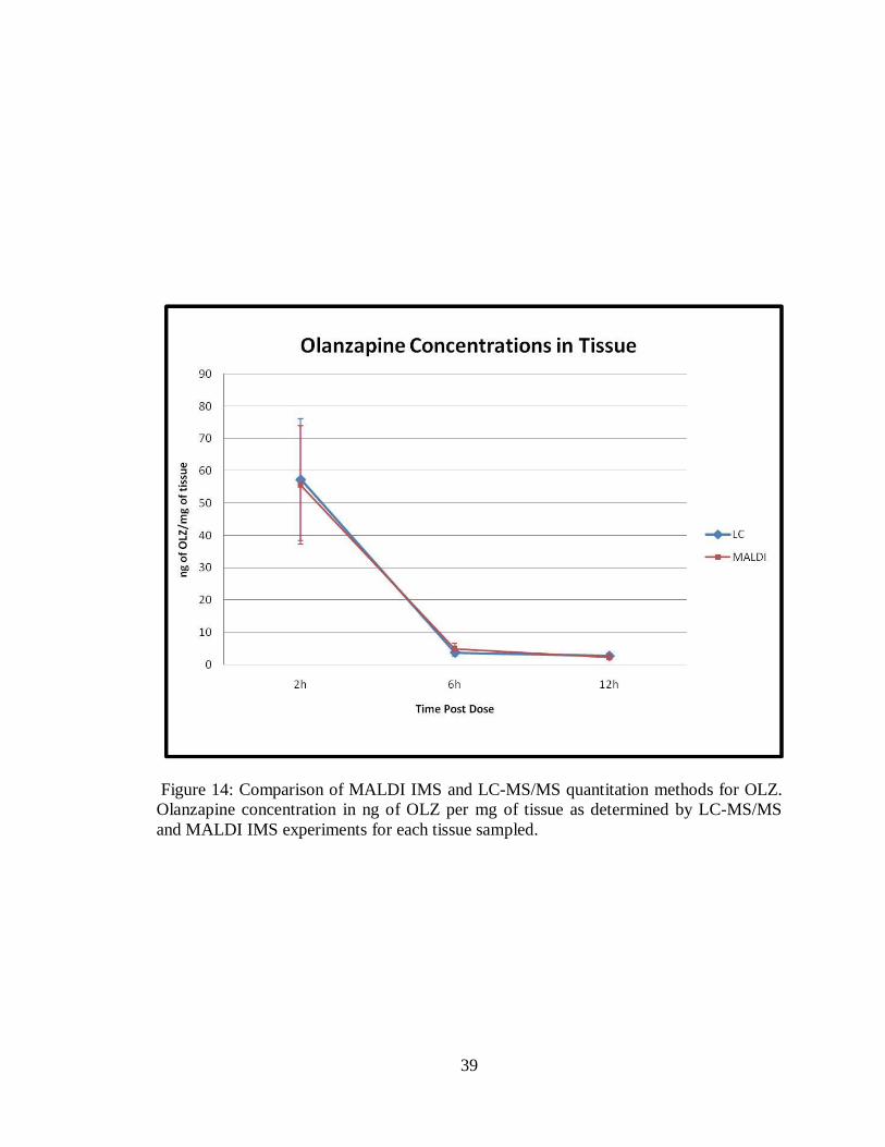
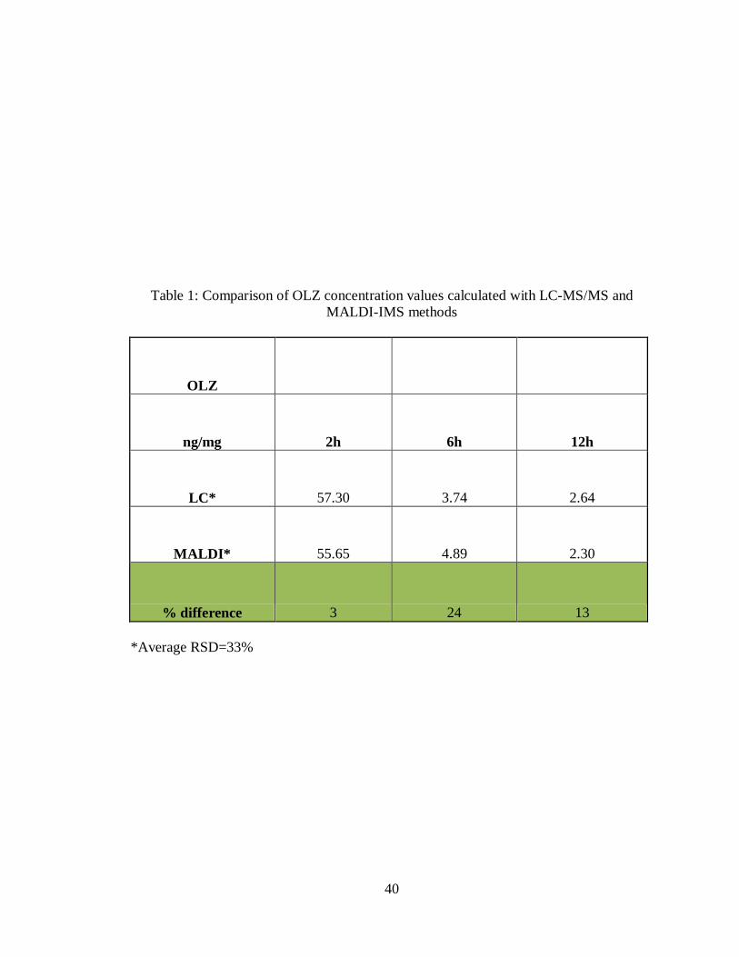
Table 1: Comparison of OLZ concentration values calculated with LC-MS/MS and

MALDI-IMS methods

OLZ

ng/mg 2h 6h 12h

LC* 57.30 3.74 2.64

MALDI* 55.65 4.89 2.30

% difference 3 24 13

*Average RSD=33%

41

Materials and Methods

Materials

The MALDI matrices, 3,5-dimethoxy-4-hydroxycinnamic acid (sinapinic acid,

SA), α-cyano-4-hydroxycinnamic acid (CHCA), and 2,5-dihydroxybenzoic acid (DHB),

were purchased from Sigma Chemical Co. (St. Louis, MO) along with sodium hydroxide

and ammonium acetate. HPLC grade acetonitrile, methanol, and hexane were purchased

from Fisher Scientific (Suwanee, GA). HPLC grade cyclohexane was purchased from

Acros Organics (Geel, Belgium). Fischer 344 rats were purchased from Charles River

Laboratory, Inc. (Wilmington, MA). Zyprexa tablets (OLZ) were obtained from the

Vanderbilt University Hospital Pharmacy (Nashville, TN). All animal studies were

approved by the Institutional Animal Care and Use Committee at Vanderbilt University.

Animal Dosing Methods

OLZ was administered per oral (p.o.) at pharmacologically relevant doses of 8

mg/kg to 10 week-old male Fischer 344 rats, which had fasted overnight prior to start of

study. Animals were euthanized at 2h, 6h and 12h post-dose by isoflurane anesthesia

followed by exsanguination via decapitation. Control and dosed brain, liver, and kidney

were harvested and frozen in powdered dry ice.

Signal Depth Methods

Fresh frozen tissue sections at 12 µm thickness were collected at -20 ºC using a

Leica CM3050s cryomicrotome (Leica Microsystems, Inc., Germany) and thaw-mounted

42

to gold-coated MALDI target plates. Sections were acquired for Olanzapine dosed rat

brain. Target plates were stored in a dessicator until analysis. Matrix solution was made

fresh at 40 mg/ml DHB in a 50% methanol solution and spiked with 2 µM of d4-

olanzapine. The matrix solution was spotted onto the tissue sections on the Portrait™

630 (Labcyte Inc.) depositing a total of 6.8 nl (40 passes, 1 drop/pass, 170 pl/drop) in a

300 µm x 300 µm spatial resolution array. Photos were acquired for the spotted tissue

sections using an Olympus BX50 microscope (Olympus Optical Co, LTD. Tokyo,

Japan,) fitted with a Micropublisher 3.3 camera (QImaging, Canada) at 10x

magnification. Once spotting was completed the plates were allowed to dry in the dark

for a minimum of 15 minutes before being introduced into the MALDI LTQ XL (Thermo

Scientific Inc.). Spectra were acquired across the array in a total of 7-14 locations per

matrix spot to get an accurate representation of the signal distribution across the entire

area. At each position spectra were acquired at 45 laser shot intervals (3 µscans/step, 15

laser shots/µscan) or at 15 laser shot intervals (3 µscans/step, 5 laser shots/µscan) with a

20 µJ laser energy. Spectra were acquired at the same absolute x and y coordinate

location until no signal was detected. Spectra were introduced to in-house software

designed by Surendra Dasari (Frappienator) to export the absolute x and y coordinates

along with the total signal intensity for a specific m/z for each spectra acquired and the

information was put into an excel spreadsheet for further statistical analysis.

Area Ablation Calculation Methods

A gold coated MALDI target was covered with a thin layer of DHB matrix by

sublimation using an in-house built sublimination chamber. Once coated the plate was

43

introduced into the MALDI LTQ XL (Thermo Scientific Inc.) for laser spot size analysis.

The laser was positioned over an area of the plate with the DHB matrix and then fired at

specified laser powers and raster patterns typically used for acquiring data. The plates

were then taken to an Olympus BX50 microscope (Olympus Optical Co, LTD. Tokyo,

Japan,) fitted with a Micropublisher 3.3 camera (QImaging, Canada) at 10x magnification

and pictures were acquired at 10x magnification. Using the microscope software, Image-

Pro Plus, the dimensions of the laser spot burn patterns were measured to determine the

size of the laser spots.

Tissue Dimension Calculation Methods

Fresh frozen tissue sections at 12 µm thickness were collected at -20 ºC using a

Leica CM3050s cryomicrotome (Leica Microsystems, Inc., Germany). One section was

thaw mounted to a glass slide while ten subsequent sections were collected on a

previously weighed piece of wax coated weigh paper. The ten sections were immediately

weighed on a micro balance to get their mass. The weight of the weigh paper was

subtracted from the total mass. This process was repeated five times for each tissue

evaluated and the average mass of a tissue section was calculated. The sections on the

slides were stained with cresyl violet and cover slipped. The stained slides were allowed

to dry and then images were acquired on a flat bed scanner at 3200dpi next to a

measurement slide. The images were imported into Adobe Photoshop software. Using

the marquee tool make a rough selection of the area of interest. Open the color range

tool. Using the Select Drop Down Menu and select Color Range. Once the dialogue box

is open, make sure the radio dial box is checked selection and the selection preview is set

44

to Black Matte. Hold down the shift button and select the various color regions needed

for area calculation. Use the Fuzziness toolbar by sliding to the right to adjust until all

areas to be used for the calculation are selected without any unwanted areas showing in

the preview window. Finalize the selection by clicking OK. Now that the area has been

selected it is necessary to find the number of pixels within the selection. This can be

done using the Histograms, located in the palates toolbar on the right hand side of the

screen. Make sure the view is in expanded mode and the show statistics button is also

selected. Number of pixels can be found in the lower left hand corner of the statistics

display. Occasionally the histrogram will show an error icon indicating that it needs to be

refreshed to calculate the pixels with uncached data. Do this by clicking the refresh

button in the upper right hand corner of the histogram dialogue box. This must be done

to ensure that an accurate pixel count is obtained. Take note of the number of pixels

selected. In order to convert the number of pixels into actual units, it is necessary to find

the number of pixels within an object in the image for which the actual real life

dimensions are known. Using the marquee tool, select the area of known dimensions as

accurately as possible. Go back to the Histograms box and obtain the number of pixels.

Now you can use the information to convert the number of pixels to physical units.

Divide the number of pixels within the unknown area of interest by the number of pixels

within the area of known dimensions. Multiply by the known dimension. This results in

the exact physical measurement for the area of interest.

45

Limits of Detection and Calibration Curve Methods

A dilution series of OLZ stock solutions was made in 100% methanol and stored

at -20oC until use. The series spanned six orders of magnitude (1 ng/ml, 10 ng/ml,

100 ng/ml, 1000 ng/ml, 10,000 ng/ml, 100,000 ng/ml) to allow for accurate limit of

detection determination. From these stock solutions a standard series was made by

adding known amounts into already prepared matrix (DHB 40 mg/ml, 50 % methanol:

50% water). One hundred µl of the appropriate stock was added to 900 µl of matrix to

make the following dilution series: 0.1 ng/ml, 1 ng/ml, 10 ng/ml, 100 ng/ml, 1,000 ng/ml

and 10,000 ng/ml. To each solution the appropriate internal standard was added to a 2

µM concentration.

Fresh frozen tissue sections at 12 µm thickness were collected at -20 ºC using a

Leica CM3050s cryomicrotome (Leica Microsystems, Inc., Germany) and thaw-mounted

to gold-coated MALDI target plates. Sections were acquired for Fisher 344 rat brain.

Plates were put into a dessicator to dry for a minimum of 60 minutes. After drying, the

plates were spotted with the standard spiked matrix dilution series on the acoustic reagent

multi-spotter (Portrait™ 630, Labcyte Inc.) 6.8 nl per spot (40 passes, 1 drop/pass, 170

pl/drop) in a 300 µm x 300 µm spatial array resulting in a 20 x 10 spot array for each

standard solution. The plates were allowed to dry in the dark for 15 minutes before being

introduced into the MALDI LTQ XL (Thermo Scientific Inc.) where spectra were

acquired. The acquisition method used a 50 µm raster at 14 different positions across the

matrix spot, 2 scan events (one for the analyte, one for the internal standard) alternated

for a total of 40 scan events per position, 3 µscans per scan event, 5 laser shots per µscan

at a laser power of 20 µJ.

46

Dosed Tissue Analysis

Fresh frozen tissue sections at 12 µm thickness were collected at -20 ºC using a

Leica CM3050s cryomicrotome (Leica Microsystems, Inc., Germany) for each OLZ

dosed brain. Plates were put into a dessicator to dry for a minimum of 60 minutes. After

drying, the plates were spotted with DHB matrix (40 mg/ml, 50% MeOH) spiked with 2

µM of d4-OLZ as an internal standard on the acoustic reagent multi-spotter (Portrait™

630, Labcyte Inc.) 6.8 nl per spot (40 passes, 1 drop/pass, 170 pl/drop) in a 300 µm x 300

µm spatial array resulting in a 20 x 10 spot array. The plates were allowed to dry in the

dark for 15 minutes before being introduced into the MALDI LTQ XL (Thermo

Scientific Inc.) where spectra were acquired. The acquisition method used a 50 µm raster

at 14 different positions across each matrix spot, 2 scan events (one for the analyte, one

for the internal standard) alternated for a total of 40 scan events per position, 3 µscans per

scan event, 5 laser shots per µscan at a laser power of 20 µJ.

Drug Quantitation Using LC-MS/MS

The extraction protocols used here were modeled after published protocols of

OLZ quantitation from dosed tissues.65-67

For each tissue being evaluated a piece of the

tissue was cut and then weighed with a minimum of 100 mg used, this was done in

triplicate. Once the tissue was weighed it was homogenized with water, 1 ml for every

100 mg of tissue used, and 3 µg of the internal standard being used. The tissue was

homogenized thoroughly until uniform by visual inspection and then the liquid was

transferred to a test tube using a Pasteur pipet. A 1:1 dilution of sodium hydroxide was

added to the tube and the solution was vortexed to pH the solution. For the extraction,

47

ten ml of cyclohexane was added to the test tube and then mixed by inversion for two

hours. The mixture was then centrifuged for 30 minutes at 3500 rpm. The organic layer

was removed and transferred into a scintillation vial which was then dried under Nitrogen

gas at 37 °C. Samples were reconstituted in 300 µl of 10mM ammonium acetate in 50%

acetonitrile and then transferred to autosampler vials. Standard curves were prepared by

spiking a control homogenate with the OLZ standard, which covered a concentration

range of 1-1000 ng/g.

Samples were analyzed on an ESI TSQ Quantum triple-quadrupole system

(Thermo Scientific, Waltham, MA) equipped with an autosampler (set at 4 ºC) and HPLC

system. A C12 Synergi MAX-RP 150 x 2 mm column (Phenomenex, Torrance, CA) was

used with a fast gradient run of mobile phase A (5:95 acetonitrile:0.5% acetic acid in

water, 10 mM ammonium acetate) to mobile phase B (95:5 acetonitrile:0.5% acetic acid

in water, 10 mM ammonium acetate).

Acknowledgements

Dr. Surendra Dasari and Dr. David Tabb developed the in-house software

(Frappienator) used to export the intensities from the MALDI LTQ XL data.

48

CHAPTER III

ANALYSIS OF IMATINIB TREATED GL26 MURINE CELL XENOGRAFTS

Overview

Glioblastoma multiforme (GBM) is the most common type of malignant primary

brain tumor with over 10,000 new cases diagnosed each year in the United States.68

Glioblastomas account for approximately 60 to 70% of malignant gliomas, anaplastic

astrocytomas for 10 to 15%, and anaplastic oligodendrogliomas and anaplastic

oligoastrocytomas for 10%; less common tumors such as anaplastic ependymomas and

anaplastic gangliogliomas account for the rest.68

Despite current methods of therapy

including surgery, radiation and chemotherapy the median survival for GBM is only 12-

18 months. However, with recent progress in understanding the molecular pathways of

this disease it is becoming possible to generate new and better therapies for treatment of

GBM. Malignant transformation in gliomas is the result of sequential accumulation of

genetic aberrations and deregulation of growth factor signaling pathways. Targeted

therapies have been developed against these pathways.69

Targeted therapy may provide

greater specificity toward tumor cells with potentially less toxicity than conventional

chemotherapy. The success of these agents in other systemic cancers demonstrates their

potential in tumors with well-defined molecular targets.70, 71

Even though the complexity

of the molecular abnormalities in GBMs and the redundancy of the signaling pathways

make it unlikely that single agents will achieve great success, there has been significant

interest in this approach.

49

Inhibition of deregulated protein kinases by small molecule drugs has evolved

into a major therapeutic strategy for the treatment of human malignancies. Knowledge

about direct cellular targets of kinase-selective drugs and the identification of druggable

downstream mediators of oncogenic signaling are relevant for both initial therapy

selection and the nomination of alternative targets in the event that molecular resistance

emerges. Protein kinases are critical regulators in human cancer and play major roles in

tumor cell proliferation, migration and survival. Aberrant kinase activity has been

identified as a major factor contributing to disease progression in various human

malignancies. The targeted inhibition of protein kinases has therefore emerged as a major

therapeutic approach and fueled the development of various kinase-selective drugs, such

as cell-permeable small molecule inhibitors, with the potential to address currently unmet

medical needs in cancer therapy.

In this project, we now seek to detect the quantitative distribution of the targeted

molecular therapy Imatinib (IMAT) and to define the biological mechanisms that govern

the ability of molecular targeted therapies to induce death of tumor cells in the brain.

The results of these studies will assist us in improving and validating future molecular

targeted therapies for malignant brain tumors.

Introduction

PDGF in Gliomas

Tyrosine kinases are a group of protein kinases critical to signal transduction

pathways involved in cell proliferation, growth, survival, adhesion, motility and

50

differentiation. The group includes receptor tyrosine kinases (RTKs) which are

transmembrane proteins containing an extracellular binding domain that binds ligands

and an intracellular kinase domain that activates intracellular signaling pathways.

Platelet derived growth factor (PDGF) is a member of this family and induces cellular

growth, proliferation and differentiation by activating intracellular signaling mechanisms

via platelet derived growth factor receptor (PDGFR).72

PDGF consists of a dimer of two

polypeptide chains, A and B with a 60% homology. They can assemble as a heterodimer

(PDGF-AB) or homodimers (PDGF-AA or PDGF-BB). The receptors are membrane

glycoproteins expressed in several tissue cells and consist of two subunits α and β

encoded by two different genes.73, 74

There are also more rare forms of PDGF being C

and D.75

All forms of PDGF and PDGFR have been found to be overexpressed in human

brain tumors such as menigiomas, astrocytomas, oligodendrogliomas, medulloblastomas,

and ependymomas and are associated with the more malignant tumors.72, 74, 75

Because of

the numerous genetic and physiological alterations observed in human glioma the

importance of PDGF signaling is still not fully understood. But PDGF autocrine loops

are thought to both initiate and sustain the transformed phenotype of glioblastoma cells.76

This notion has experimental support. Glioma-like tumors can be induced in mice after

overproduction of PDGF in mouse brain. Also, some glioma-derived cell lines have been

blocked by interference with PDGF receptor signaling.77

Imatinib

Imatinib is a small molecule drug used for the treatment of some cancers. It is

known to inhibit PDGFR-α, PDGFR-β, Bcr-Abl, c-Fms, and c-kit tyrosine kinases.78

As

51

described in the previous section dysregulated PDGFR kinase activity has been linked to

a variety of cancers, including glioblastoma. 72, 74, 75

IMAT has been shown, in animal

models, to enhance the antitumor effects of chemotherapeutic agents due to inhibition of

PDGFR phosphorylation and therefore may have potential efficacy as an adjuvant

therapy.79

The mechanism of action is thought to be growth delay through growth arrest

in the G0-G1 phase rather than inducing apoptosis. IMAT inhibits the autocrine PDGFR

stimulation which leads to decreased cell population.76, 79

Use of Animal Models

In order for scientists to fully understand how cancers develop, spread through the

body and discover new and effective ways of diagnosis and treatment, it is necessary to

carry out research on live animals. Animal studies are essential to understand the

complexities of the biological processes that are involved in cancer within living

organisms. They are also required before any trials for new drugs can begin in humans.

While the use of nonhuman animal models is a common component of biomedical

research, the role of animal models in research, its scientific and ethical justification and

legal regulations and policies need to be considered before any project can begin.80, 81

Approval and animal protocols must be submitted and approved by the Institutional

Animal Care and Use Committee (IACUC).82

Careful consideration also needs to be

taken to ensure that the animal model selected will biologically represent the disease or

condition that you are investigating.

When designing a MALDI IMS experiment it is important to select the proper

small animal model. In the early phases of drug discovery and development, therapeutic

52

candidates cannot be administered to humans, and therefore, predictions about the PK/PD

properties have to be made from an in vivo animal model. The two most common species

include rats and mice, which have different metabolic rates and pathways; hence

providing vastly different metabolite and distribution information. In general, rats are

used for PK/PD studies due to their similarity to human pathways to determine the

ADME of an administered pharmaceutical. In other cases, mice may be preferred, since

many more models of disease are available in mice rather than rats.83

Taking all of this

into consideration a syngenic mouse GL26 glioma model was chosen. It has been shown

that GL26 experimental murine gliomas share most characteristic histological features

with human gliomas.84

Results

Animal Implantation and Drug Dosing

To start the study two sets of mouse implantations and drug dosing were done.

One set was used to evaluate the effects of chronic dosing of the imatinib. For this set of

experiments 25 mice were implanted with GL26 cultured tumor cells and tumor growth

was allowed to occur for 12 days. (Extra mice were implanted to take into account any

casualties.) On day 12 the IMAT treatments began and continued for six days. Group

one was the control group dosed once a day for six days with saline solution (p.o.).

Groups two through five were dosed once a day with 100 mg/kg IMAT (p.o.) for 1 day

(1d), 2 days (2d), 4 days (4d) and 6 days (6d) respectively. Twenty-four hours after the

53

final dose the mice were sacrificed, the brains were excised, immediately flash frozen in

liquid nitrogen and stored at -80 °C.

The second set of mice was to evaluate the effects of a single imatinib dose over

time. Five groups of five mice each were evaluated for a treatment response. 30 mice

were implanted with GL26 murine tumor cells and tumor growth was allowed to occur

for 12 days. (Extra mice were implanted to take into account any casualties.) On the

12th day mice were given a single dose of 100 mg/kg IMAT (p.o.) and then sacrificed in

groups according to the time point they would represent. Groups were sacrificed 2 hours

(2h), 6 hours (6h), 12 hours (12h) or 24 hours (24h) after the administration of the IMAT

dose. Control mice were sacrificed 24 hours after a dose of saline solution (p.o.). The

brains were excised and immediately flash frozen in liquid nitrogen and stored at -80 °C.

Drug Detection and Quantitation

When deciding to use a treatment for a particular disease, one of the most

important things to investigate is whether or not the compound is getting to the area that

needs to be treated. To this end, the distribution of IMAT was determined in tumor

bearing mouse brain tissues to elucidate if the drug was penetrating through the Blood

Brian Barrier (BBB) or the Blood Tumor Barrier (BTB). The BBB is the bottleneck in

brain drug development and is the single most important factor limiting the future growth

of neurotherapeutics.85

Sections for analysis were cut on a cryostat at 12 µm and then prepared for

MALDI IMS accordingly by applying DHB matrix with d8-IMAT internal standard

using a Portrait™ 630 (Labcyte Inc). All sections were analyzed on a MALDI LTQ XL

54

(Thermo Scientific, Inc.) monitoring the major collision induced fragment of IMAT at

m/z 394.1. To display the images, the data was input into Biomap and then normalized to

the d8-IMAT internal standard by taking the ratio of the IMAT signal over the d8-IMAT

signal at each location. IMAT signal was detected very strongly from the tumor area of

the mouse brain with much less signal coming from the normal brain tissue (Figure 15).

The MALDI images are shown in the grey boxes and below are the scanned images of

Hemotoxylin and Eosin (H&E) stained serial sections of mouse brain tissue. These

images show that the IMAT is penetrating into the brain mainly in the tumor region.

Various tissue types can have different ionization effects, so to determine if the

image results were an effect of differing ionization efficiencies standard solutions were

analyzed on both the normal and tumor tissue types. DHB matrix was made in 50%

methanol with 2 µM of d8-IMAT as an internal standard. IMAT standard was then spiked

into aliquots of the matrix resulting in concentrations of 10000 ng/ml and 1000 ng/ml.

The spiked matrix was spotted on both the tumor bearing portion of a non-dosed brain

and also the non-tumor bearing areas of the tissue resulting in matrix spots that contained

68000 fg of IMAT and matrix spots with 6800 fg of IMAT. Spectra were acquired from

each of the spots and the intensities were recorded. There was not a significant increase

or decrease in the control or tumor regions intensities for the IMAT or d8-IMAT signals

and no significant differences of the IMAT/d8-IMAT ratios. The percent difference

between standard intensity ratios from the tumor and normal regions was below 5%.

Table 2 shows the IMAT/d8-IMAT ratio averages taken from the matrix spots containing

either 68000 or 6800 fg of IMAT. Both the tumor and normal regions show the same

ionization efficiency for the IMAT signal. These results indicate that the signal

55

differences seen between the tumor and normal areas of the dosed brain images are not

due to a difference in ionization effects of the tissue but are true differences in the amount

of IMAT present in the tissues.

Figure 15: IMAT images taken on a MALDI LTQ XL monitoring for CID fragment

m/z 394.1. A) A tumor bearing mouse brain dosed with a saline solution. The grey box

contains the MALDI image and below is an H&E stained section of the mouse brain. B)

A tumor bearing mouse brain dosed with IMAT. The grey box contains the MALDI

image and below is an H&E stained serial section of the mouse brain.

MALDI images were acquired for each of the brains within the respective dosing

groups. For the acutely dosed mice it can be seen that the IMAT signal is strong at 2h

post dose in the tumor regions and is at its highest concentration 6h post dose. From

there the amount of detected IMAT decreases at the 12h and 24h post dose time-points as

56

Table 2: IMAT/d8-IMAT signal ratios taken from standards spotted on tumor and normal

tissues within a mouse brain

68,000 fg of IMAT 6,800 fg of IMAT

Normal 22.29 ± 0.69 %RSD=3.12 2.69 ± 0.07

%RSD=2.64

Tumor 21.19 ± 0.91 %RSD=4.32 2.66 ± 0.10

%RSD=3.78

% Difference 4.9 1.1

seen in Figure 16. For the chronically dosed samples the amount of detected IMAT is

relatively constant in the normal regions of the brain tissue but there is an increase of

IMAT signal in the tumor region after 4d and 6d of continued treatment shown in Figure

17.

With the images providing a qualitative assessment for the amount of IMAT

present in each of the dosing groups, experiments needed to be performed to

quantitatively assess the absolute IMAT concentration in the brain tissues. This was

accomplished by following the MALDI quantitation protocol developed in Chapter II and

outlined in Appendix A. First 12 µm sections were collected from each brain and

weighed on a microbalance immediately following sectioning. A 12 µm GL26 implanted

brain section had an average mass of 0.64 mg with an 8% RSD. Brain sections were then

stained and scanned using a flatbed scanner at 3200 dpi to provide images for tissue area

57

Figure 16: Imatinib images for the acutely dosed mouse brain samples. The top-most

row shows the imatinib distribution for a representative brain at each acute time-point

(images acquired on the Thermo MALDI LTQ). The bottom row displays the H&E

stained section for the representative brains.

Figure 17: Imatinib images for the chronically dosed mouse brain samples. The top-

most row shows the imatinib distribution for a representative brain at each chronic time-

point (images acquired on the Thermo MALDI LTQ). The bottom row displays the H&E

stained section for the representative brains.

58

calculation. The images were imported into Adobe Photoshop and the area of a 12 µm

GL26 implanted brain section was determined to be 62.37 mm2 with a 0.6% RSD. The

area of the laser to be used for spectra acquisition was determined to be 0.0035 mm2

(Chapter II) and using this information the amount of tissue sampled within one laser

position can be calculated: 62.37 mm2/0.64 mg = 0.0035 mm

2/ X mg. The amount of

tissue sampled is 3.59x10-5

mg. Next, a calibration curve of IMAT was constructed.

Matrix solutions were spiked with IMAT to yield final concentrations of 100, 10, 1, 0.1

ng/ml along with 2 µM of d8-imatinib as the internal standard. Using the Portrait™ 630,

matrix was deposited onto non-dosed brain tissue sections in known volumes resulting in

680, 68, 6.8 and 0.68 fg of IMAT along with a blank standard of matrix only with

internal standard. Spectra were acquired from each of the spots, using 600 laser shots per

position and 14 positions per matrix spot. This totaled 140 different laser positions for

each standard due to the fact that ten matrix spots per calibration standard were analyzed.

For each matrix spot the total signal of the IMAT and the d8-IMAT was summed using

in-house software (Frappienator) and the ratio of IMAT/d8-IMAT was taken. The ratios

for each calibration standard were plotted and a linear fit was calculated. Each point on

the curve had a RSD no higher than 25% and the curve had excellent linearity with an R2

value of 0.9996 as shown in Figure 18. From this curve, the LOD of imatinib with this

acquisition method by MALDI, was determined to be approximately 20 ng/g of tissue.

IMAT dosed tissue sections were cut for each brain and spotted with DHB in 50%

methanol spiked with 2 µM of d8-IMAT as an internal standard. From each dosed

section 140 positions were analyzed totaling 5600 spectra for each brain. The average

ratio of IMAT/d8-IMAT signal was taken for each time-point and plugged into the

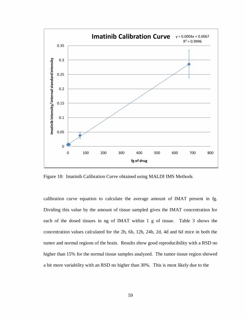
59

Figure 18: Imatinib Calibration Curve obtained using MALDI IMS Methods

calibration curve equation to calculate the average amount of IMAT present in fg.

Dividing this value by the amount of tissue sampled gives the IMAT concentration for

each of the dosed tissues in ng of IMAT within 1 g of tissue. Table 3 shows the

concentration values calculated for the 2h, 6h, 12h, 24h, 2d, 4d and 6d mice in both the

tumor and normal regions of the brain. Results show good reproducibility with a RSD no

higher than 15% for the normal tissue samples analyzed. The tumor tissue region showed

a bit more variability with an RSD no higher than 30%. This is most likely due to the

y = 0.0004x + 0.0067R² = 0.9996

0

0.05

0.1

0.15

0.2

0.25

0.3

0.35

0 100 200 300 400 500 600 700 800

Imat

inib

inte

nsi

ty/

inte

rnal

sta

nd

ard

inte

nsi

ty

fg of drug

Imatinib Calibration Curve

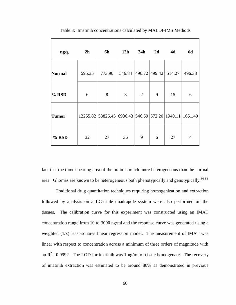
60

Table 3: Imatinib concentrations calculated by MALDI-IMS Methods

ng/g 2h 6h 12h 24h 2d 4d 6d

Normal 595.35 773.90 546.84 496.72 499.42 514.27 496.38

% RSD 6 8 3 2 9 15 6

Tumor 12255.82 53826.45 6936.43 546.59 572.20 1940.11 1651.40

% RSD 32 27 36 9 6 27 4

fact that the tumor bearing area of the brain is much more heterogeneous than the normal

area. Gliomas are known to be heterogeneous both phenotypically and genotypically.86-88

Traditional drug quantitation techniques requiring homogenization and extraction

followed by analysis on a LC-triple quadrapole system were also performed on the

tissues. The calibration curve for this experiment was constructed using an IMAT

concentration range from 10 to 3000 ng/ml and the response curve was generated using a

weighted (1/x) least-squares linear regression model. The measurement of IMAT was

linear with respect to concentration across a minimum of three orders of magnitude with

an R2= 0.9992. The LOD for imatinib was 1 ng/ml of tissue homogenate. The recovery

of imatinib extraction was estimated to be around 80% as demonstrated in previous

61

studies.89, 90

Samples of tissue from both tumor and normal tissues of the brain for each

dosing group were prepared and then analyzed. Using the response curve, average

imatinib concentrations were found for each dosing group and are shown in Table 4. As

with the MALDI results, the RSD for the normal samples was around 15% and the tumor

samples around 30%, again speaking to the higher heterogeneity of the tumor tissue.

Table 4: Imatinib concentrations calculated by LS-MS/MS Methods

ng/g 2h 6h 12h 24h 2d 4d 6d

Normal 542.31 710.48 401.92 355.26 240.54 357.12 361.32

% RSD 11 6 14 16 8 16 16

Tumor 6099.49 11632.86 1492.48 243.34 377.72 733.95 570.20

% RSD 33 5 9 35 15 6 11

The quantitation results for both the MALDI and the LC methods were plotted on

a line graph for comparison. Figure 19 shows the IMAT concentrations in ng/g (ng of

IMAT per g of tissue) for the acutely dosed mouse groups, 2h, 6h, 12h and 24h. The blue

trace represents the results obtained by LC-MS/MS and the red trace represents the

62

results obtained by MALDI-IMS. The tumor tissue results are plotted on a graph

separately (top graph) from the normal tissue results (bottom graph). The values

calculated using the MALDI method are higher in all instances than the values calculated

using the LC method with a percent difference between the two methods as low as 30%

for the tumor samples and 8% for the normal samples. Figure 20 shows the IMAT

concentrations in ng/g (ng of IMAT per g of tissue) for the mice dosed chronically, 1d,

2d, 4d, and 6d. The tumor (top graph) and normal (bottom graph) results are plotted

separately with the blue trace representing the LC-MS/MS results and the red trace

representing the MALDI-IMS results. Here again the MALDI results are all higher than

those of the LC results. Across all of the samples the average percent difference between

the two methods is 40% with the results from the MALDI being higher in all instances.

Looking at the plotted data, the MALDI and LC results follow the same trends of drug

concentration across the different dosing groups.

Proteome Response Study

In order to evaluate for a pharmacodynamic response to the imatinib presence in

the tumor bearing portion of the brains, each brain was imaged by MALDI-TOF MS.

Standard MALDI imaging preparation steps were employed to get the samples ready for

analysis. Samples were cut on a cryostat, thaw mounted onto target slides, dried and then

matrix application was performed on a Portrait™ 630 spotter before imaging on a Bruker

Autoflex TOF MS. Three sections were analyzed for each brain and sample acquisition

was randomized to eliminate bias. Serial sections were cut for each brain and stained

according to a standard cresyl violet staining protocol. These stained sections were

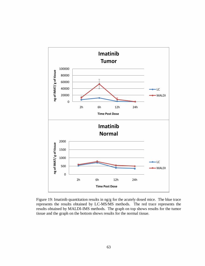
63

Figure 19: Imatinib quantitation results in ng/g for the acutely dosed mice. The blue trace

represents the results obtained by LC-MS/MS methods. The red trace represents the

results obtained by MALDI-IMS methods. The graph on top shows results for the tumor

tissue and the graph on the bottom shows results for the normal tissue.

0

20000

40000

60000

80000

100000

2h 6h 12h 24h

ng

of

IMA

T/ g

of

tiss

ue

Time Post Dose

ImatinibTumor

LC

MALDI

0

500

1000

1500

2000

2h 6h 12h 24h

ng

of

IMA

T/ g

of

tiss

ue

Time Post Dose

ImatinibNormal

LC

MALDI

64

Figure 20: Imatinib quantitation results in ng/g for the chronically dosed mice. The blue

trace represents the results obtained by LC-MS/MS methods. The red trace represents the

results obtained by MALDI-IMS methods. The graph on the top shows results for the

tumor tissue and the graph on the bottom shows results for the normal tissue.

0

500

1000

1500

2000

2500

3000

1d 2d 4d 6d

ng

of

IMA

T/ g

of

tiss

ue

Days of Dosing

ImatinibTumor

LC

MALDI

0

500

1000

1500

2000

1d 2d 4d 6d

ng

of

Imat

/ g

of

tiss

ue

Days of Dosing

ImatinibNormal

LC

MALDI

65

scanned on a Mirax Scanner (Carl Zeiss MicroImaging) and the images were saved.

After acquisition of the MALDI images it was possible to import, co-register and overlay

the stained image with the MALDI image and optical image of the spotted section using

Flex Imaging software (Bruker Daltonics, Germany). This allowed for the visualization

of all the MALDI images and for spectra from specific regions in the brain to be selected

and saved into separate folders for further processing and statistical analysis. With the

assistance of a neuro-oncologist, the tumor bearing areas of the brain tissue were

identified and spectra from these areas were extracted. Figure 21 shows the co-

registration and spectra selection process.

Figure 21: Workflow for extracting regions of spectra from an image data set. A)

Optical image of a matrix spotted brain section B) Scanned image of a cresyl violet

stained serial brain section C) Co-registrated overlay of the optical and stained image.

Red outlined areas indicate where spectra were selected from the tumor region of the

brain and put into a folder. Black outlined areas indicate where spectra were selected

from the normal region of the brain and put into a folder. These folders of spectra then

underwent spectral processing procedures and statistical analysis.

MALDI IMS analysis was performed on a total of 40 brains, with three sections

being imaged for each brain. This resulted in 120 sections analyzed and approximately

10,000 spectra acquired. From each brain section 15 or more spectra were selected from

66

the tumor region so that there were a minimum of 45 spectra representing each brain and

225 spectra representing each dosing group.

All spectra were processed using ClinPro Tools, commercially available software

from Bruker Daltonics (Germany). Once the spectra had undergone baseline subtraction,

smoothing, normalization, realignment and peak picking the data for each spectrum was

exported collectively into a feature table (a list of each m/z value and its corresponding

intensity value for each spectrum). Using these feature tables, various analyses and

statistical tests were performed to evaluate the protein changes that occurred with respect

to amount of IMAT present.

The feature tables generated from ClinPro Tools were put into the program

MiniTab® (MiniTab Inc., State College, Pennsylvania) to create interval plot of each m/z

value as its analyte signal progressed from the dosing group with low drug concentration

to the dosing group with the most IMAT presence. Figure 22 shows example interval

plots for m/z 4195 and 14422. These plots provided a visual inspection of the m/z trends

as a result of drug concentration. Once imported into MiniTab® and interval plots had

been reviewed, one-way analysis of variance (ANOVA) statistical analysis was computed

for each m/z. An ANOVA algorithm tests the hypothesis that the means of several

populations are equal. A one-way ANOVA can be used to tell you if there are

statistically significant differences among the level means. The null hypothesis for the

test is that all population means (level means) are the same. The alternative hypothesis is

that one or more population means differ from the others. ANOVA measures two

sources of variation in the data and compares their relative sizes using the F-statistic

finding the variance between the groups in relation to the variation within the groups. A

67

Figure 22: Example Interval Plots created in the MiniTab® software program. A)

Interval Plot of m/z 4195 demonstrating an increase in signal intensity going from no

IMAT presence in the samples to a high concentration of IMAT in the samples. B)

Interval plot of m/z 14422 demonstrating a decrease in signal intensity going from low to

high IMAT concentrations.

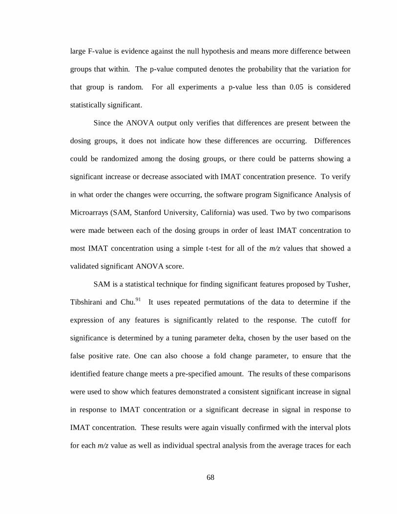
68

large F-value is evidence against the null hypothesis and means more difference between

groups that within. The p-value computed denotes the probability that the variation for

that group is random. For all experiments a p-value less than 0.05 is considered

statistically significant.

Since the ANOVA output only verifies that differences are present between the

dosing groups, it does not indicate how these differences are occurring. Differences

could be randomized among the dosing groups, or there could be patterns showing a

significant increase or decrease associated with IMAT concentration presence. To verify

in what order the changes were occurring, the software program Significance Analysis of

Microarrays (SAM, Stanford University, California) was used. Two by two comparisons

were made between each of the dosing groups in order of least IMAT concentration to

most IMAT concentration using a simple t-test for all of the m/z values that showed a

validated significant ANOVA score.

SAM is a statistical technique for finding significant features proposed by Tusher,

Tibshirani and Chu.91

It uses repeated permutations of the data to determine if the

expression of any features is significantly related to the response. The cutoff for

significance is determined by a tuning parameter delta, chosen by the user based on the

false positive rate. One can also choose a fold change parameter, to ensure that the

identified feature change meets a pre-specified amount. The results of these comparisons

were used to show which features demonstrated a consistent significant increase in signal

in response to IMAT concentration or a significant decrease in signal in response to

IMAT concentration. These results were again visually confirmed with the interval plots

for each m/z value as well as individual spectral analysis from the average traces for each

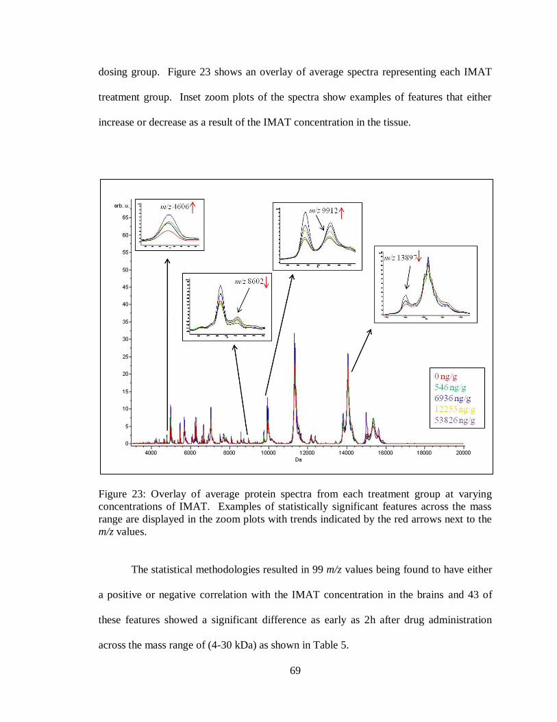
69

dosing group. Figure 23 shows an overlay of average spectra representing each IMAT

treatment group. Inset zoom plots of the spectra show examples of features that either

increase or decrease as a result of the IMAT concentration in the tissue.

Figure 23: Overlay of average protein spectra from each treatment group at varying

concentrations of IMAT. Examples of statistically significant features across the mass

range are displayed in the zoom plots with trends indicated by the red arrows next to the

m/z values.

The statistical methodologies resulted in 99 m/z values being found to have either

a positive or negative correlation with the IMAT concentration in the brains and 43 of

these features showed a significant difference as early as 2h after drug administration

across the mass range of (4-30 kDa) as shown in Table 5.

70

Table 5: Statistically significant features affected by IMAT presence

m/z Trend Fold

Change

SAM

score

ANOVA

p-value

ANOVA

F Score

ANOVA

R-Sq

AUC

4195 up 1.7 9.8 < 0.005 48.67 16.54 0.90

4445 up 1.4 3.8 < 0.005 6.09 2.42 0.70

4606 up 2 7.5 < 0.005 17.54 6.67 0.76

4682 up 1.4 7.7 < 0.005 30.07 10.91 0.85

4710 up 1.5 4.6 < 0.005 17.17 6.54 0.85

4768 up 2.1 6.4 < 0.005 14.29 5.5 0.69

4901 up 1.4 4.5 < 0.005 13.41 5.18 0.76

4965 up 1.8 7.7 < 0.005 22.81 8.5 0.73

5143 up 1.6 5.5 < 0.005 16.09 6.15 0.72

5172 up 2.2 6 < 0.005 18.77 7.1 0.71

5445 up 1.4 8 < 0.005 25.71 9.48 0.83

6345 down 1.2 -2.9 < 0.005 41.20 14.37 0.78

6547 up 1.5 7.6 < 0.005 31.99 11.53 0.84

6574 up 1.5 10.7 < 0.005 39.98 10.92 0.91

7108 down 1.3 -7.2 < 0.005 47.15 16.11 0.78

7750 down 1.2 -7.5 < 0.005 64.87 20.9 0.63

7793 up 1.2 6.1 < 0.005 22.18 8.28 0.85

7829 up 1.4 4.1 < 0.005 10.78 4.31 0.75

7858 up 1.3 4.2 < 0.005 18.88 6.76 0.74

7891 up 1.4 5.2 < 0.005 21.26 7.97 0.73

7933 up 1.9 5.9 < 0.005 28.,23 10.31 0.80

8602 down 1.2 -5.3 < 0.005 38.48 13.55 0.66

9071 up 1.3 3.1 < 0.005 18.24 6.92 0.68

9203 up 1.2 3.1 < 0.005 4.40 1.62 0.70

9534 up 1.4 3.2 < 0.005 7.26 2.87 0.73

9638 up 1.2 3.3 < 0.005 17.60 6.69 0.71

9701 up 1.5 5.5 < 0.005 18.38 6.97 0.79

9740 up 1.8 11.9 < 0.005 23.32 8.68 0.92

9777 up 1.2 3.8 < 0.005 32.36 11.65 0.68

9912 up 1.3 7.2 < 0.005 28.20 9.94 0.77

10256 down 1.3 -6.5 < 0.005 19.27 6.9 0.60

10640 up 1.3 3.5 < 0.005 17.06 6.5 0.70

10953 up 1.6 5.7 < 0.005 37.72 13.32 0.74

11309 down 1.2 -7.6 < 0.005 36.72 13.01 0.50

11337 down 1.2 -8.6 < 0.005 56.83 18.47 0.57

11517 down 1.7 -21.7 < 0.005 107.82 30.52 0.96

11841 down 1.3 -5.7 < 0.005 27.19 9.97 0.62

12203 down 1.3 -7.9 < 0.005 69.88 22.16 0.66

12285 down 1.4 -7.7 < 0.005 50.20 16.98 0.75

13897 down 1.3 -8.7 < 0.005 42.31 14.07 0.83

14053 down 1.1 -4.1 < 0.005 8.75 3.44 0.57

14422 down 1.4 -10.8 < 0.005 47.17 16.12 0.73

71

For the table the first column lists the m/z values that were found to be significant

followed by the trend up or down relative to the increasing amount of IMAT presence in

the second column. The third column lists the fold change which represents the maximum

change found between the two group extremes in the data set; between the samples with

no IMAT presence and the samples with the maximum amount of IMAT presence in the

tissues. This value was calculated by the SAM analysis along with a SAM score which is

shown in column four. The score assigned to each m/z value was based on the change in

expression relative to the standard deviation of repeated measurements. It is the

standardized change in expression. A positive SAM score means that there is an increase

of the signal going from group one to group two, the opposite is true for a negative SAM

score.

The next three columns list the results from the ANOVA test. The p-value

computed denotes the probability that the variation for that group is random. For all

experiments a p-value less than 0.05 was considered statistically significant. The F-Score

represents the results from the F-statistic stating that there was more difference between

groups that within the groups. A larger F-Score indicates a stronger confidence. The

ANOVA R-sq is often referred to as the coefficient of determination and is a measure of

the „goodness of fit‟ of the regression model. If R-sq equals zero, then there is no linear

relationship between the dependent and independent variables; if R-sq equals 1, the

relationship is perfect and all values of the dependent and independent variables lie on a

straight line.

The AUC values listed in the final column were obtained from a Receiver

Operating Characteristic (ROC) curve for each peak. It is an evaluation of the

72

discrimination quality of a peak. The area under the ROC curve (AUC), measures

discrimination, which is the ability of the test to correctly classify two groups. In this

instance the AUC is the score between the samples with the least IMAT concentration

and the samples with the most IMAT concentration. Thus, the AUC measures the ability

of a particular m/z to discriminate the two groups. The closer the area is to 0.5, the less

useful the test is, and the closer it is to 1.0, the better the test is. This test was performed

in the ClinProTools (Bruker) software.

MALDI IMS produces mass specific data of the intact protein species; however,

the m/z alone is often not sufficient to positively identify the protein, as the biologically

active protein may have undergone post-translational modifications. Robust protein

identification is routinely achieved through protein separation/isolation, proteolytic

digestion, sequencing of peptides by LC MS/MS, and matching the peptides to genome-

based protein databases. The MALDI peaks confidently identified using these strategies

are shown in Table 6. The molecular weight (MW) and corresponding protein

identifications are listed along with the percent coverage, modifications, SwissProt

Identification number, the number of peptides identified, peptide residues sequenced, and

the protein trend as affected by the concentration of IMAT present.

Discussion

From the image data it can be determined that the IMAT is getting to the tumor,

crossing the BTB, but there is substantially less IMAT penetrating into the normal, non-

invaded, parts of the brain through the BBB. In previous studies it has been shown that

the permeability of the BTB is greater than that of the BBB.92, 93

BBB and BTB

73

Table 6: Protein Identifications for tumor implanted mouse brains treated with imatinib

Protein Name

% coverage

of

unprocessed

precursor

Modifications

(amino acid

chain)

Swissprot

Primary

Accession

Number

Number

of

Peptides

Peptide

Residues

covered Trend

4964 Thymosin beta-4 38 *(8-50) P20065 1 27-45 up

6546

40S ribosomal protein

S29 19 (2-56) P62274 5 34-40, 49-56 up

7829

cAMP-dependent

protein kinase inhibitor

alpha 48 (2-76) P63248 2 21-58 up

7890

Guanine nucleotide

binding protein

G(1)/G(S)/G(0) subunit

gamma-13 13 *(2-67) Q9JMF3 2 45-54 up

9202

Cytochrome c oxidase

subunit 7A2 25 *(2-83) P48771 2 34-56 up

9637

Cytochrome b-c1

complex subunit 8 54 (2-82) Q9CQ69 3

11-25, 49-71,

74-82 up

9911

Acyl-CoA-binding

protein 34 *(2-87) P31786 5 34-53, 73-83 up

10255 ATP synthase subunit f 24 *(2-88) P56135 2 17-39 down

10639 Protein S100-B 15 *(2-92) P50114 2 7-21, down

10952

Protein S100-A111

(Calgizzarin) 16 (2-98) P50543 2 8-18, 51-57 up

11336 ATP synthase subunit g 36 *(2-103) QPCPQ8 3

12-24, 36-54,

96-103 down

11516 cytochrome c, somatic 32 *(2-105) P62897 5 29-39, 40-56,

93-100 down

11840

FK506-binding protein

1B 23 *(1-108) Q9Z212 2 2-14, 59-72 down

12202 Snrpf protein 17 (1-112) Q6NZQ3 2 92-99, 100-112 down

13896 Small nuclear

ribonucleoprotein D3 13 *(2-126) Q91VM2 3 55-64, 70-78 down

14052 Beta-synuclein 37 (1-133) Q91ZZ3 5 33-84 down

14421 Bol A like protein 1 26 *(1-137) Q9D8S9 3

22-37, 40-52,

77-85 down

*acetylated N-terminus (+42 Da)

permeability measured by quantitative autoradiography (QAR) shows that the BTB has a

Ki value of 12 while the Ki value of the BBB averages at 3. (The Ki value is the

unidirectional transfer constant (µl/g/min) of a [14

C] labeled tracer.)92

In another study

brain metastasis uptake of 14

C-paclitaxel and 14

C-doxorubicin was generally greater than

74

normal brain.93

There is general agreement that most chemotherapy agents achieve only

relatively low concentrations in the normal central nervous system, that the blood-brain

barrier is variably disrupted in malignant brain tumors, and that the concentration of

chemotherapy drugs in the brain adjacent to tumor is intermediate between

concentrations achieved in brain tumors versus normal brain. Average drug

concentrations in brain adjacent to tumor are lower than those within brain tumors94

This

difference in BTB and BBB permeability would explain why the IMAT signal is much

stronger in the tumor region of the brain. This is also supported by a study that shows the

IMAT can reach significant intratumoral concentrations in patients with glioblastoma

multiforme and a disrupted BBB.95

The IMAT shows no signal in the control tissues, very high signal at 2h and then

reaches its most intense at 6h. Following that at 12h and 24h the signal decreases. It has

been shown that IMAT is rapidly absorbed after oral administration with peak plasma

concentrations between 2h-6h having maximum plasma concentrations of 0.921 ± 0.095

μg/ml (mean ± S.D., n = 4).96

Following that the terminal elimination half life was

determined to be 13.5 ± 0.9 h.96

IMAT is extensively distributed into tissues and highly

protein bound, predominantly to albumin and α1-glycoprotein (AGP).97

The image

results correspond to the previous studies of IMAT absorption with highest signal

intensities between 2h and 6h then drastically decreasing at 12h and 24h. In the chronic

dosed tissues there is little signal in the 1d, 2d, and then increased signal in the 4d and 6d

samples indicating there is an additive effect of the IMAT with chronic treatment. By

continually taking a drug a steady-state of the drugs concentration can be reached and this

is optimal for maximum efficiency of the treatment. It takes somewhere between 5 and 6

75

half-lives for a drug to reach steady state.98

With the half-life of IMAT being around 12h

it would be expected that by day 6 the IMAT presence in the brain has reached its steady

state concentration.

Using the newly developed MALDI-MS/MS methods (Chapter II), the absolute

concentration of the IMAT in the brain tissues was able to be calculated. When

compared to the results obtained with the LC-MS/MS results there is an average percent

difference of 40% with the MALDI results consistently higher in every instance. Part of

the difference is most likely due to the fact that the recovery of the LC IMAT extraction

was around 80%, so there is drug lost through the extraction process. There could have

also been drug lost as a result of the IMAT sticking to the HPLC column during analysis.

Another explanation could be that for the LC method, the entire tissue section analyzed is

homogenized thereby averaging the entire tissue‟s drug concentration for the sample. For

the MALDI, the spatial integrity is maintained, and the spots selected for analysis each

receive their own IMAT concentration calculation and thus could represent areas of

higher concentration locally than the average of the entire tissues concentration. Despite

the higher concentrations calculated by the MALDI-IMS method, the trends of

concentration from dosing group to group remains the same for both the MALDI and LC

results.

Detection and identification of changes in the proteome of glioma as a result of

targeted molecular therapies provides invaluable insights into the drug‟s activity.

Typically, the proteins affected by IMAT administration are not extensively known.

Many drug effects occur primarily when the blood level of the drug is either going up or

down. When the drug reaches a steady state, these effects can be attenuated or

76

completely absent. Therefore the most drastic changes will be seen in the samples with

most varied levels of IMAT present as within the acutely dosed sample set.

A number of protein signals were found to have either increased or decreased

signal intensities as a result of the IMAT presence. A group of these proteins are found

to be involved in the mitochondrial electron transport chain (ETC). Cytochrome c

oxidase subunit 7a2 (part of complex IV) and cytochrome b-c1 complex subunit 8 (part

of complex III) were found to have an increase in intensity as the concentration of IMAT

increased, while cytochrome c and ATP synthase subunits f and g (parts of complex V)

had a decrease in intensity. Adaptive response to agents that challenge cellular

homeostasis involves important changes in mitochondrial function. Given their crucial

role in cell physiology, mitochondria are among the first responders to various stressors.99

The ETC or respiratory system occurs in the cristae of the mitochondria, where a

series of membrane associated complexes, cytochromes and coenzymes, mediate

biochemical reactions to produce ATP. These cytochromes and coenzymes remove

electrons from the donor, NADH, and pass them to a terminal electron acceptor, O2 via a

series of redox reactions. The reactions create a proton gradient across the mitochondrial

inner membrane, resulting in the transmembrane proton gradient used to make ATP via

ATP synthase in oxidative phosphorylation.100

The process of electron transport consists

of four complexes. Complex I, which consists of NADH dehydrogenase (synonym:

NADH-ubiquinone oxidoreductase), removes two electrons from NADH and transfers

them to the carrier, ubiquinone. Simultaneously, Complex I moves four protons across

the membrane to produce a proton gradient later used to generate ATP through oxidative

phosphorylation. Complex II, which consists of succinate dehydrogenase, funnels

77

electrons into the quinone group by removing electrons from succinate and transferring

them via FAD to the quinone. Complex III (cytochrome bc1 complex) removes two

electrons from the quinone and transfers them to two molecules of cytochrome c, a water-

soluble electron transporter located on the outer surface of the membrane.

Simultaneously, Complex III moves two protons across the membrane, producing a

proton gradient consisting of four total protons. When electron transfer is somehow

hindered in Complexes I and III, there is a tendency for premature electron leakage to

oxygen, resulting in the formation of superoxide. Complex IV, consists of cytochrome c

oxidase. It is responsible for removing four electrons from the four molecules of

cytochrome c and transferring them to O2, producing two molecules of water.

Simultaneously, it also moves four protons across the membrane, producing a proton

gradient. Finally, this proton gradient is utilized by the ATP synthase complex, also

known as complex V to make ATP via oxidative phosphorylation.

The changed intensities of the proteins associated with the ETC can possibly be

explained by evaluating the mechanisms of resistance to RTK inhibition such as

antiapoptotic mechanisms. The mechanisms of resistance to RTK inhibition have not

been fully elucidated, but is has been shown that tumor cells unresponsive to EGFR

inhibitors are characterized by reduced induction of apoptosis. 101

Furthermore, while

IMAT dramatically increases apoptosis in BCR-ABL–positive chronic myelogenous

leukemia and in gastrointestinal stromal tumors, it does not induce apoptosis when

administered to glioblastoma cells either in vitro or in vivo, even at high

concentrations.76, 102

Antiapoptotic mechanisms that render glioma cells resistant to

78

cytotoxic agents (chemotherapy and radiotherapy) may also modulate their response to

targeted therapies such as RTK inhibitors.103

A recent study into the chemoresistance of temozolamide (TMZ) showed that

there were changes involving ETC. They explored changes in paired patient samples

both before and after TMZ treatment. They found that complex II, III, and IV activities

increased significantly (p = 0.0005) along with a significant decrease in complex I and V

activity.104

Considering that the cytochrome c/complex III molar ratio is the minimum

needed for complex III activity105, 106

an increase in complex III activity will likely

decrease the pool of cytochrome c available for release from the mitochondrion to initiate

apoptosis. This would explain why after the administration of IMAT there is an increase

in the subunits associated with complexes III and IV of the ETC and a decrease in the

cytochrome c and ATP synthase subunits (complex V) intensity in the tumor samples

shown here. With this information, targeted experiments to elucidate the exact function

of these proteins and how they could possibly be linked to treatment resistance and anti-

apoptotic functions after administration of IMAT in gliomas can be investigated.

S100B is another protein that is affected by IMAT presence. There is a decrease

in S100B protein intensity as the IMAT concentration increases in the tumor areas.

S100B is a Ca2+

-binding protein of the EF-hand type that is abundantly expressed in

astrocytes and has been implicated in the regulation of several intracellular activities,

including proliferation and differentiation. S100B might contribute to reduce the

differentiation potential of cells of the astrocytic lineage and participate in the astrocyte

activation process in the case of brain insult and in invasive properties of glioma cells.

Astrocytes represent the brain cell type with the highest expression of S100B. Levels of

79

S100B also increase in gliomas, raising the possibility that the protein might have a role

in glioma pathophysiology.107, 108

Studies have demonstrated that inhibition of S100B

production in glial cells is correlated with at least three phenotypic changes: (a) a more

flattened cellular morphology; (b) an alteration in cytoskeletal organization at the level of

the microfilament network; and (c) a decrease in cellular growth rate.109

Results obtained

with two distinct antisense methods support the conclusion that S100B has important

roles in regulation of glial cell morphology, cytoskeletal structure, and cell proliferation.

Thus, a decrease in S100B intensity could indicate that IMAT mechanisms inhibit S100B

and therefore create a decrease in the tumors cellular growth rate.

Another affect of increased IMAT concentration in the tumor tissue was a

decrease in beta-synuclein intensities. β-synuclein is a synuclein protein found primarily

in brain tissue and is seen mainly in presynaptic terminals. β-synuclein is predominantly

expressed in the neocortex, hippocampus, striatum, thalamus, and cerebellum.110

The γ-

synuclein protein has been found to be abnormally expressed in a high percentage of

tumor tissues of cancer types, including liver, gastric, lung, prostate, cervical etc.111

and

α-synuclein has been implemented in a number of neurodegenerative disorders.112

Synucleins have also been found to be expressed highly in glial tumors113

and although

their exact function is not yet known they are known to be involved in cellular functions

including synaptic plasticity, neurofilament organization, control of dopamine

homeostasis and vesicular transport.114

Many other identified proteins were also affected by the IMAT concentrations

although not all of the functions in glioma tissues have been completely elucidated.

Small nuclear ribonucleoprotein D3 intensities are decreased at high concentrations of

80

IMAT in tissue. Small nuclear ribonucleoprotein particles have been shown to have an

integral role in pre-mRNA splicing.115

Global aberrant alternative pre-mRNA splicing

has been indicated as an epigenetic phenomenon in cancer and specifically independent.

In silico genome-wide assessments have identified genes expressing particular splice

isoforms more frequently in glioma than in normal brain.116

BolA like protein 1 has a

decreasing intensity at high concentrations of IMAT. The BolA-like proteins seem to be

involved in cell proliferation or cell-cycle regulation, but the molecular function is still

unknown.117

Acyl CoA binding protein shows an increase in intensity and is known to

bind medium- and long-chain acyl-CoA esters with very high affinity and may function

as an intracellular carrier of acyl-CoA esters. In vitro and in vivo experiments suggest

that it is involved in multiple cellular tasks including modulation of fatty acid

biosynthesis, enzyme regulation, regulation of the intracellular acyl-CoA pool size,

donation of acyl-CoA esters for β-oxidation, vesicular trafficking, complex lipid

synthesis and gene regulation.118

In summary, the MALDI MS data obtained in this study were able to provide 43

molecular features associated with IMAT concentration in the brain tumors. Correlating

IMAT distribution to proteome response in the brain MALDI MS analyses provided a

means to directly correlate drug distribution with pharmacological response and provided

insight into the concentration-effect relationship. Further work needs to be performed to

determine the identity of all the molecular features altered in order to rationalize the

biological significance of these proteins. Evaluating some of the proteins already

identified, many molecular processes including ETC, proliferation, cell cycle regulation

and pre-mRNA splicing have been found to be affected by the administration of IMAT.

81

Additional experiments can delve further into these functions and provide more

information on the efficacy of IMAT, reveal additional drug targets, and help elucidate

the mechanisms of the drug action on the brain tumors. Additionally, the MALDI-IMS

techniques provide a rapid, reproducible method to find the IMAT drug concentrations in

tissue while maintaining spatial integrity.

Materials and Methods

Materials

The MALDI matrices, sinapinic acid and 2,5-dihydroxybenzoic acid, tissue

staining chemicals cresyl violet acetate, hemotoxylin and eosin, and ammonium acetate

were purchased from Sigma Chemical Co. (St. Louis, MO). Acetic acid, HPLC grade

acetonitrile, ethanol, methyl-tert-butyl ether (MTBE) and MeOH were purchased from

Fisher Scientific (Suwanee, GA). Trifluoroacetic acid (TFA) and hydrochloric acid (HCl)

was purchased from Burdick and Jackson (Muskegon, MI). Dulbecco‟s Phosphate-

Buffered Saline (D-PBS), Dulbecco‟s modified eagle medium (DMEM), fetal calf serum,

penicillin-streptoycin, Tissue Protein Extraction reagent (TPER), phosphate buffer

solution (PBS), tricine gels, reducing agent, See Blue, Novex Tricine SDS Running

Buffer, trypsin, 0.05% with EDTA and Colloidal Blue Staining kit were purchased from

Invitrogen (Carlsbad, CA). Trypsin gold was purchased from Promega (Madison, WI).

Imatinib was acquired from the Vanderbilt Research Pharmacy in 100 mg tablets

(Nashville, TN). Imatinib and d8-imatinib were provided as their mesylate salts by Dr.

Jeremy Norris (Protein Discovery, Knoxville, TN). GL26 murine glioma cells were

82

acquired from Vanderbilt University (Dr. Moneeb Etesham‟s laboratory, Nashville, TN).

C57BL/6NCr female mice were purchased from Charles River Laboratories

(Wilmington, MA). Animal sedatives xylazine, ketamine, and buprenorphine were

purchased from Lloyd laboratories (Shenandoah, Iowa).

Cell Culturing

Cryogenically frozen GL26 murine glioma cells were obtained from the

Neurology Department Brain Tumor Bank at Vanderbilt University. The cells were

thawed and then placed in DMEM containing 10% fetal calf serum, and 1% penicillin-

streptomycin. Aseptic cell culturing technique as described119

was employed to continue

the cell line growth and cells were maintained in humidified incubators gassed with 5%

carbon dioxide. Prior to injection, GL26 cells were harvested, washed twice in PBS,

counted, and adjusted to 100,000 cells per µl of DPBS in an eppendorf tube.

Tumor Implantation

From their time of arrival at the animal facility, each animal was housed

undisturbed to acclimate to the new environment for a period ranging from 1-3 days.

Food, Purina 5001 rodent diet, and water were provided ad libitum to animals upon

arrival and throughout the study. After the acclimation period, animals were taken to the

procedure room for survival surgery to implant the GL26 murine tumor cells

intracranially. The survival surgery involved the establishment of intracerebral brain

tumors in the mice. To achieve this, animals were first anesthetized. For administration

of the anesthesia the animals were held by hand while the brief injection was made

83

directly above the hind limb on the underbelly of the animal (intraperitoneal injection) of

200 µl (0.019 ml/g of weight) of a mixture of xylazine (2.2%) and ketamine (6.5%).

After administration the animals were immobilized in a stereotactic frame, and received

an intracranial injection (2 µl, approximately 200,000 cells) of the GL26 brain tumor

cells (resuspended in DPBS) into the brain. This necessitated the placement of a midline

incision in the scalp followed by creation of a burr hole (using a high-speed dental drill)

in the skull at the site 2.5 mm lateral to bregma where the tumor injection was to take

place. Tumor cells were injected at a depth of approximately 2.5 mm below the surface of

the skull. The injection was done very slowly (1 µl/min), and then the needle was left in

place for 2 min before removal to avoid liquid reflux. The syringe was removed and the

scalp incision was closed with wound clips. All techniques were performed using

sterilized instruments and the wound was created and closed using aseptic procedure. In

the postoperative period it was expected that these techniques impart pain on the animal.

To address this, animals received a subcutaneous injection of buprenorphine (0.05 - 1.0

mg/kg) prior to the animal waking up from anesthesia. They then received an additional

injection of buprenorphine 8-12 hours after the first injection due to the possibility of

further postoperative pain. Animals were placed on a thermal blanket during surgery to

ensure maintenance of body temperature and were kept under a physiological heat lamp

after surgery while they were recovering from anesthesia. Following recovery, animals

were placed back in their cages, returned to the vivarium, and monitored daily for signs

of infection or distress. After ten days, once the scalp incision had healed, the wound

clips were removed.

84

Animals were monitored daily for a period ranging from 15-20 days to allow for

tumor growth to occur. After this period select animals that had been designated for drug

dosing were handled and received a non-toxic and physiologically relevant dose of drug

as determined by the experiment being performed.

Operative mortality will likely occur within 48-72 hours of surgery; these animals

will be removed from the analysis. As a 10-12.5% mortality has been reported using this

procedure, one additional animal per treatment group per experimental replicate was

implanted.

Drug Dosing

Imatinib was obtained from the Vanderbilt Research Pharmacy in the form of a

100 mg tablet. These are the same tablets that patients would receive if prescribed

IMAT. Tablets were dissolved in water at a pH=4 (water made acidic with the addition

of HCl) resulting in a 10 mg/ml drug solution. IMAT is readily soluble at acidic pH

values (≤ 5). The solution was vortexed for five minutes to ensure that the entire quantity

of IMAT was dissolved. The IMAT solution was stored at -4 °C for no longer than 48

hours before fresh solution was made. The drug placebo administered was water at pH=4

(made acidic with the addition of HCl).

For oral gavage the animal was held by hand while tipping the head up to allow

the insertion of the oral gavage blunt tipped needle into the mouth and down toward the

stomach. Once the needle was in place approximately 300 µl of the drug solution

(resulting in a 100 mg/kg dose) were administered to the animal. After administration the

needle was slowly removed from the mouth and the animal was immediately released.

85

Tissue Preparation and MALDI Imaging

After all dosing had been completed the animals were taken to be sacrificed.

Each animal was put under anesthesia, (110 mg/kg Ketamine and 10 mg/kg Xylazine)

through intraperitoneal injection as a single dose followed by spine dislocation and

immediate decapitation. Brain tissues were excised from the C57/BL/6 mice using sterile

dissection techniques and immediately flash frozen in liquid nitrogen. All tissues were

kept at -80 °C until further use.

Frozen brain tissues were mounted onto a cryostat chuck with OTC. Tissue was

trimmed until an even sagittal section was acquired at Interaural 10.6 mm, Bregma 1.6

mm, where the corpus callosum has started to join at the mid-line of the brain. From this

position tissue sections (12 µm) were collected, one for protein analysis, a serial section

for IMAT analysis and a serial section for H&E staining. Sections for protein and IMAT

analysis were mounted onto gold-coated MALDI targets while the sections for staining

were thaw mounted onto charged glass microscope slides.

For cresyl violet staining, 0.5% cresyl violet was made by adding 2.5 g of cresyl

violet acetate to 250 ml of distilled water and 1.5 ml of acetic acid. The solution was

stirred for 20 minutes and then filtered. After sections had been mounted onto the

charged glass slides, they were dipped briefly, approximately 5 seconds, into water. The

slides were then dipped into the 0.5% cresyl violet for 45 seconds, rinsed briefly with

water and rinsed with 100% ethanol for 20 seconds. Slides were then placed into Xylene

for 5 minutes followed by cover-slipping with cytoseal.

For H&E staining, slides were dipped in a series of solutions to re-hydrate,

dehydrate and stain the tissue sections. 30 seconds in 95% ethanol. 30 seconds in 70%

86

ethanol. 30 seconds in Milli-Q water. 2 minutes in hematoxylin solution (deep purple;

stains nuclear contents). 20 seconds in Milli-Q water. 30 seconds in 70% ethanol. 30

seconds in 95% ethanol. 1 minute in eosin solution (pink; stains cytoplasm). 30 seconds

in 95% ethanol. 30 seconds in 100% ethanol. 2-2.5 minutes in Xylene. To cover-slip,

dry the back of the microscope slide and around the tissue section with a Kimwipe to get

rid of excess xylene. Put 1-3 drops of cytoseal on the tissue section and then place a

coverslip over area. Make sure to get rid of air bubbles and let the cytoseal dry until

hardened.

MALDI targets were placed into a desiccator for at least an hour to dry. To

prepare sections for imatinib imaging a matrix solution of DHB (40 mg/ml, 50% MeOH)

was prepared with 2 µM d8-imatinib as the internal standard. Sections were spotted on

the Portrait (Flyby 1 drop 40 repeats) at 300 µm x 300 µm spatial resolution. All

IMAT images were acquired on a MALDI-LTQ XL. The MALDI target with sections

designated for protein analysis was reagent washed (70% reagent alcohol for 30 seconds,

70% reagent alcohol for 30 seconds, 100% reagent alcohol for 15 seconds, air dried).

The surface of the sections were then seeded with finely ground SA. Fresh SA matrix

solution was made in 60% acetonitrile 40% water 0.02% TFA. The sections were spotted

using the Portrait (Flyby 1 drop 30 repeats) in a 300 µm x 300 µm array. The MALDI

target was scanned and sections were imaged on an Autoflex (Bruker Daltoniks).

Data Pre-Processing

Data analysis generally lies in two categories; pre-processing and statistical

analysis. It is important to assess reproducibility of the mass spectra so that variations in

87

peak intensities can be correlated to biological endpoints. The pre-processing step

reduces the experimental variance between spectra through the removal of background,

normalization of the peak intensity to the total ion current, and peak alignment

algorithms. Normalization of the spectra minimizes variation arising from day to day

instrument fluctuations, differences in matrix crystallization across tissue sections, and

changes in sample preparation and chemical properties of the underlying tissue 120

.

Various algorithms are employed for all of the spectra processing steps; baseline

subtraction, smoothing, peak alignment, normalization and peak picking. Ion images are

generated directly from these processed data sets.

For each image acquired, the corresponding stained serial section was co-

registered and with the assistance of a neuro-oncologist the spectra from the tumor

bearing regions were exported. Spectra from each section were kept together in separate

folders. These folders were then input into ClinPro Tools where the imported spectra

were processed with the following parameters; 1200 Resolution, data reduction factor of

5, Top Hat baselining with 10% Minimal Baseline Width, Savitsky Golay Smoothing

enabled at 2 width 10 cycles, recalibration 2000 ppm max peak shift with 20% match to

calibrate peaks excluded not recalibratable spectra, from m/z range 4000-20,000, and null

spectra exclusion. Once spectra were imported into ClinPro Tools and processed, peak

selection was performed (peak picking on total avg spectrum, SN=2, 0% relative

threshold to the base peak) and peak list feature tables were output.

Protein Identification

88

Tissues were homogenized in TPER supplemented with protease inhibitors. For

each extract, a Vydac C8 polymeric reversed-phase column (3.2 x 150mm) fractionated

300 g of protein solution (96 min linear gradient from 2-90 plate). During separation, a

liquid handling robot moves the transfer capillary sequentially into each of the 96 wells at

1 min intervals. To identify wells containing proteins of interest in an automated process,

0.2 L was removed from each well, mixed with SA matrix, and analyzed by MALDI-MS

(Bruker Autoflex). Fractions containing m/z values of interest were run on a gel (10-

20tricine) and bands of interest were excised and digested with trypsin gold (Promega;

Madison, WI). In solution trypsin digest was also performed on fractions which contained

m/z values of interest. A non-linear quadrupole high capacity trap (Bruker HCT Plus)

was used to analyze digested proteins. The peptides were separated on a packed capillary

column, with C18 resin (Monitor C18, 5 m; Column Engineering, Ontario, CA), using a

linear gradient (5MS/MS spectra were initially analyzed by searching the mouse

International Protein Index database using Sequest software). Protein IDPicker software

(David Tabb and Bing Zhang laboratories in the Vanderbilt University Medical Center

department of Biomedical Informatics) was then used to determine the probability that a

protein had been correctly identified, based on the available peptide sequence evidence.

Drug Quantitation Using LC-MS/MS

Standards of IMAT and d8-IMAT were prepared as stock solutions in methanol.

Calibration standards were made by adding the stock solutions to control brain tissue

homogenate to yield final concentrations of 3000, 1000, 500, 100, 25, 10, 1 ng/ml.

89

Tissue specimens were homogenized with PBS in a ratio of 1:4 (mg/µl) using a glass

homogenizer until uniform by visual inspection. A minimum of 30 mg of tissue was used

to prepare the homogenate, which was then transferred to eppendorf tubes before being

centrifuged at 3000 g for ten minutes. Fifty microliters of the supernatant was combined

with 25 µl of internal standard (d8-imatinib, 1000 ng/ml) and then the protein was

precipitated by adding 250 µl of acetonitrile/ethanol/acetic acid (90/10/0.1) with mixing

by inversion for 20 minutes. Samples were then centrifuged at 4000 g for ten minutes to

remove the precipitant. After centrifugation, the supernatant was transferred to glass

autosampler tubes and dried in a vacuum centrifuge for two hours at 40 °C and then

reconstituted in 75 µl of 50% methanol containing 0.05% ammonium acetate.

Chromatographic separation was performed using a Waters XTerra RP® C18

reverse phase column (2.1 x 100 mm, 5 µm particle) with a column heater (50 °C) and

autosampler (4 °C) on an HPLC system. The system was held at 90% MeOH for two

minutes then a linear gradient of MeOH and water, both with 0.5% ammonium acetate

was increased from 20% to 90% MeOH over two minutes and held at 90% MeOH for

two minutes before the column was then washed with a solution containing 70%

acetonitrile, 20% MTBE and 10% water of the course of five minutes, going from 0 to

100% over two minutes and maintaining at 100% for three minutes. The system was then

returned to initial conditions over two minutes and equilibrated for two minutes before

beginning the next run. The total run time was 14 minutes per sample at a flow rate of

0.5 ml/min. Ten microliters of sample were injected using a 10 µl PEEK loop and

subsequently analyzed on an ESI TSQ Quantum triple-quadrupole system (Thermo

Scientific, Waltham, MA).

90

Acknowledgements

Dr. Michael Edgeworth assisted with the GL26 mouse implantation and dosing

along with the pathological determination of tumors in the stained images. Dr. Moneeb

Ehtesham provided the use of the animal surgical room. Larry Pierce provided the cryo-

frozen GL26 cells. Deming Mi assisted with the statistical analysis.

91

CHAPTER IV

ANALYSIS OF CYCLOPAMINE TREATED DIRECT HUMAN GLIOMA CELL

IMPLANTED MOUSE XENOGRAFTS

Overview

Despite recent advances in therapeutic techniques, the prognosis for patients with

malignant brain tumors remains grim. The lethality of this disease process stems in part

from the highly invasive nature of these tumors. Microscopic nests of tumor cells

intersperse themselves with normal brain tissue, often at significant distance from the

main tumor mass. Due to their large number and varied location, current treatment

strategies are unable to specifically eliminate these tumor reservoirs in their entirety,

leading to eventual tumor recurrence.

One possible means of targeting disseminated tumor within the brain is the use of

targeted molecular therapies. It has previously been demonstrated that targeted molecular

therapies are capable of directly or indirectly inducing tumor-cell death in various cancer

models. The previous chapter investigated one of these therapies (IMAT). These

findings point to the potential that MALDI IMS technologies are useful in evaluating

treatment of malignant brain tumors.

Little is currently understood regarding the biological pathways and mechanisms that

govern the effects of these molecular compounds on tumor cells. The elucidation of these

pathways will be critical in order to better understand and optimize this highly promising

92

therapeutic strategy for brain cancer. In this project, we now seek to detect the

quantitative distribution of the targeted molecular therapy cyclopamine and to define the

biological mechanisms that govern the ability of molecular targeted therapies to induce

death of tumor cells in the brain.

Introduction

Sonic Hedgehog Pathway in Gliomas

Sonic Hedgehog (Shh) is a member of the Hedgehog (Hh) family of secreted

glycoproteins, which affect the development of many organs and cell groups. In

mammals, there are three known Hh family members; Sonic, Desert and Indian Hh.

They are involved in the development of many tissues and organs, including skin, lung,

brain, bone and blood. Shh is the most widely expressed.121, 122

In the central nervous

system, Hh signaling is critical for early ventral patterning of the neural tube along the

entire neuroaxis and later on for the development of the dorsal brain, including that of the

cerebellum and neocortex.123, 124

Hh acts by inhibiting a 12-pass transmembrane protein

called Patched1 (Ptc1) which normally inhibits a 7-pass transmembrane protein called

Smoothened (Smo). Activating Smo sends a signal intracellularly through intricate

mechanisms by a complex of proteins, to ultimately lead to the action of the zinc finger

Gli transcription factors.125

When this pathway is activated or maintained

inappropriately, various tumors can develop, including those in skin, muscle and brain.

Numerous studies have now shown that Shh signaling is essential for glioma cancer stem

cell self-renewal and cancer stem cell-initiated brain tumor growth.121, 125-127

Inhibition of

93

the hedgehog pathway however, kills these cancer stem cells and can prevent cancer from

growing and developing which could lead to a very effective stem cell targeted therapy

for gliomas.

Cyclopamine

Cyclopamine (CYC) is a teratogen that has been isolated from the lily Veratrum

californicum. It is a member of the steroidal jerveratrum alkaloids. CYC was originally

given its name due to the birth defects it caused in sheep giving them one eye. Much

interest in CYC has developed, owing to its ability to inhibit the Shh pathway resulting in

the inhibition of tumor growth and tumor progression.128-131

CYC acts by targeting Smo,

which inhibits its activity in the absence of Ptc1, thereby turning off the Hh pathway and

stopping the malignancy growth source.

Direct Human Cell Xenograft Animal Models

Typically animal models used in the investigation of cancer involve the

transplantation of mouse or rat tumor cells into a host of the same species and strain.132,

133 Growth of human (xenogeneic) tumor cells can be achieved using immunodeficient

(nude or SCID) mice to prevent rejection.134, 135

Most transplantable tumors are

established subcutaneously but more complex models may involve orthotopic

transplantation at appropriate primary sites.136

There is an increasing trend to establish

xenograft tumors directly from human cancer stem cells, to avoid artificial selection of

cells in tissue culture and changes in gene expression and phenotype, which this may

induce.137-139

These transplants may better model the principal cancer under

94

investigation, by more accurately representing the tumor architecture, heterogeneity,

expression of certain targets and response to therapy.140

Glioma cells are known to

undergo phenotypic and genotypic transformation in culture, however tumor stem cells

derived directly from primary glioblastomas have extensive similarities to normal neural

stem cells and recapitulate the genotype, gene expression patterns, and in vivo biology of

human glioblastomas.141

Results

Animal Implantation and Drug Dosing

To begin the study, a series of mouse implantations with human tumor cells and

sub sequential drug dosing was performed. Nod-scid immunodeficient mice were used

and orthotopically implanted with glioma tumor stem cells derived directly from human

biopsy tissue. The cells were never subjected to culture and were obtained by

homogenizing the tumor samples directly, dissociating with papain, and passing the

homogenate through a 40 μm filter. Cells were labeled with a CD133/1 antibody cross-

linked to magnetic nanoparticles and subjected to immunomagnetic cell separation using

the EasySep Magnetic Selection Kit.130

Three primary tumor specimens were used to

result in the following xenografts, an anaplastic ganglioglioma (X-302-AG), a high-grade

astrocytoma (X-312-HGA) and a primary glioblastoma multiforme (X-406-GBM).

Recapitulation of malignant glioma pathological features was observed and included

infiltrative growth, invasion of the corpus callosum to the contralateral hemisphere and

pleomorphic nuclei with mitotic figures.130

When compared to the GL26 murine cell

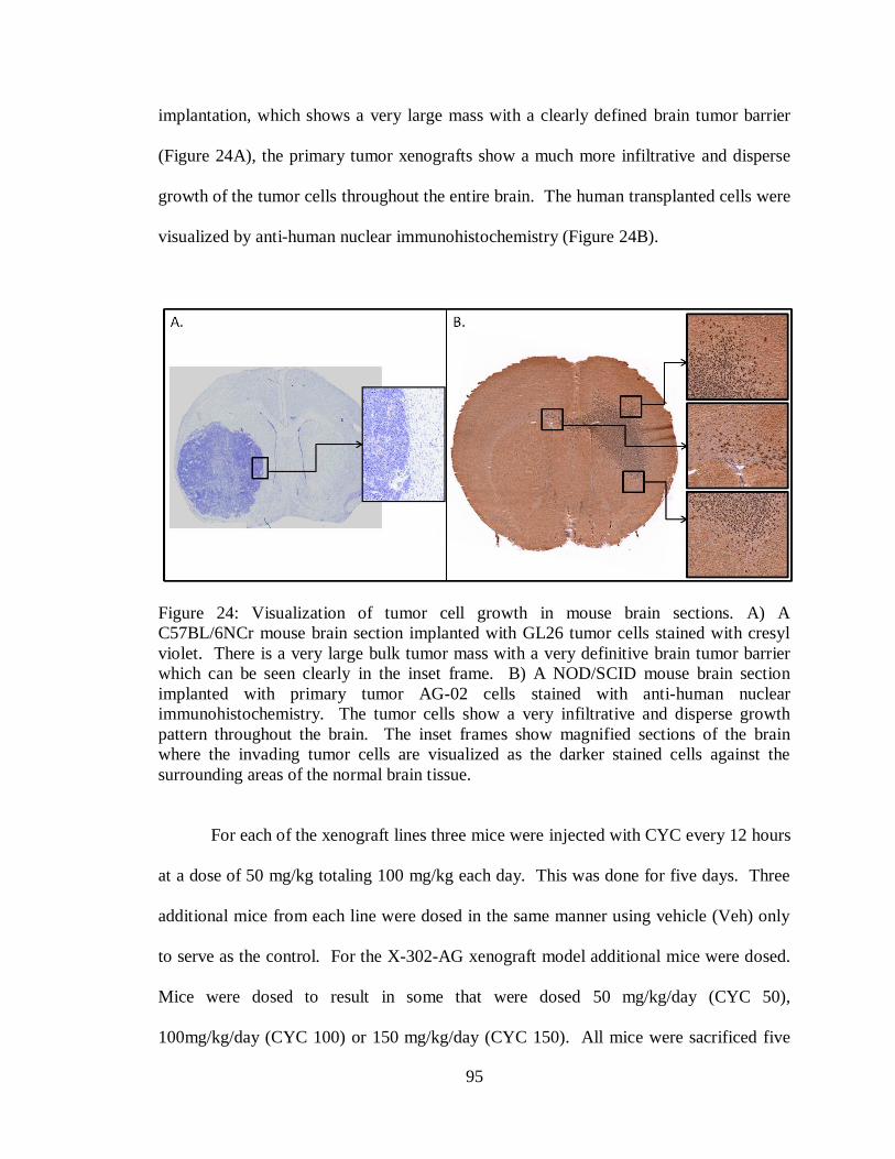
95

implantation, which shows a very large mass with a clearly defined brain tumor barrier

(Figure 24A), the primary tumor xenografts show a much more infiltrative and disperse

growth of the tumor cells throughout the entire brain. The human transplanted cells were

visualized by anti-human nuclear immunohistochemistry (Figure 24B).

Figure 24: Visualization of tumor cell growth in mouse brain sections. A) A

C57BL/6NCr mouse brain section implanted with GL26 tumor cells stained with cresyl

violet. There is a very large bulk tumor mass with a very definitive brain tumor barrier

which can be seen clearly in the inset frame. B) A NOD/SCID mouse brain section

implanted with primary tumor AG-02 cells stained with anti-human nuclear

immunohistochemistry. The tumor cells show a very infiltrative and disperse growth

pattern throughout the brain. The inset frames show magnified sections of the brain

where the invading tumor cells are visualized as the darker stained cells against the

surrounding areas of the normal brain tissue.

For each of the xenograft lines three mice were injected with CYC every 12 hours

at a dose of 50 mg/kg totaling 100 mg/kg each day. This was done for five days. Three

additional mice from each line were dosed in the same manner using vehicle (Veh) only

to serve as the control. For the X-302-AG xenograft model additional mice were dosed.

Mice were dosed to result in some that were dosed 50 mg/kg/day (CYC 50),

100mg/kg/day (CYC 100) or 150 mg/kg/day (CYC 150). All mice were sacrificed five

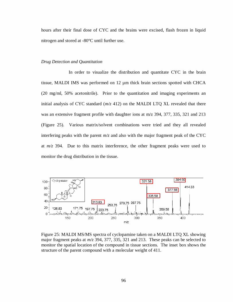
96

hours after their final dose of CYC and the brains were excised, flash frozen in liquid

nitrogen and stored at -80°C until further use.

Drug Detection and Quantitation

In order to visualize the distribution and quantitate CYC in the brain

tissue, MALDI IMS was performed on 12 µm thick brain sections spotted with CHCA

(20 mg/ml, 50% acetonitrile). Prior to the quantitation and imaging experiments an

initial analysis of CYC standard (m/z 412) on the MALDI LTQ XL revealed that there

was an extensive fragment profile with daughter ions at m/z 394, 377, 335, 321 and 213

(Figure 25). Various matrix/solvent combinations were tried and they all revealed

interfering peaks with the parent m/z and also with the major fragment peak of the CYC

at m/z 394. Due to this matrix interference, the other fragment peaks were used to

monitor the drug distribution in the tissue.

Figure 25: MALDI MS/MS spectra of cyclopamine taken on a MALDI LTQ XL showing

major fragment peaks at m/z 394, 377, 335, 321 and 213. These peaks can be selected to

monitor the spatial location of the compound in tissue sections. The inset box shows the

structure of the parent compound with a molecular weight of 411.

97

Using the MALDI small molecule quantitation protocol developed in Chapter II,

the tissue sections from X-302-AG mouse brains were analyzed. First, 12 µm sections

were collected from each brain and weighed on a microbalance immediately following

sectioning. A 12 µm Nod/Scid mouse brain section had approximately the same weight

as a C57Bl/6NCrl mouse brain section (Chapter III) weighing 0.68 mg with a RSD of

4%. Brian sections were then stained and scanned using a flatbed scanner at 3200 dpi to

provide images for the tissue area calculation. The images were imported into Adobe

Photoshop and the area of the section was determined to be 62.44 mm2 with a RSD of

0.2% which was approximately the same area as the C57Bl/6NCrl mouse brain sections.

In Chapter II the area of the laser spot was found to be 0.0035 mm2, so the amount of

tissue sampled within one laser position was calculated from the equation: 62.44

mm2/0.68 mg = 0.0035 mm

2/X mg. The amount of tissue sampled was 3.81 x 10

-5 mg.

A calibration curve for CYC was constructed by spiking CHCA (20 mg/ml 50%

acetonitrile) with CYC standard to yield final concentrations of 6800, 680, 68, 6.8 and

0.68 fg along with a blank matrix control. All solutions were spiked with 2 µM of jervine

(JERV), which served as the internal standard for the experiments. Spectra were

acquired from each of the spots, using 600 laser shots per position and 14 positions per

matrix spot. This totaled 140 different laser positions for each standard due to the fact

that 10 matrix spots per calibration standard were analyzed. For each spot the total signal

intensity was summed for both the CYC and JERV using in-house software and the ratio

of CYC/JERV was calculated. The ratios for each calibration standard were plotted and a

linear fit was calculated. Each point on the curve had a RSD no higher than 27% and the

curve had excellent linearity with an R2 value of 0.9999 (Figure 26).

98

Figure 26: Cyclopamine Calibration Curve constructed using MALDI IMS methods

From this curve the LOD of cyclopamine with this acquisition method by MALDI was

determined to be approximately 1650 ng/g of tissue.

Tissue sections for the Veh, CYC 50, CYC 100 and CYC 150 X-302-AG mice

were cut at 12 µM. The sections were spotted with CHCA in 50% Acetonitrile spiked

with 2 µM JERV internal standard. Due to the infiltrative nature of the tumor cells

within the brain, matrix spots were analyzed from various regions in the brain to get a

representation of the amount of drug present in the tissue. A total of ten matrix spots were

analyzed for each tissue with 14 positions per spot totaling 140 positions for each brain.

The ratio of total CYC signal intensity over total JERV signal intensity was calculated

and plugged into the calibration curve equation to calculate the amount of CYC present in

y = 0.0001x + 0.07R² = 0.9999

0

1

2

3

4

5

6

7

8

9

10

0 10000 20000 30000 40000 50000 60000 70000 80000

Cyc

lop

amin

e in

ten

sity

/ in

tern

al s

tan

dar

d in

ten

sity

fg of drug

Cyc Calibration Curve

99

fg. The amount of CYC was divided by the amount of tissue sampled to provide the

CYC concentration for each tissue analyzed in ng of CYC within 1 mg of tissue. The

Veh and CYC 50 tissue samples were below the limits of detection and therefore the

concentration of CYC were unable to be calculated by the MALDI method. However,

the CYC 100 tissues had a concentration of 2937 ng/g with a RSD of 26.7% and the

CYC 150 tissues had a concentration of 12333 ng/g with a RSD of 15.1% (Table 7).

Table 7: Comparison of cyclopamine concentrations calculated by both LC-MS/MS and

MALDI-IMS methods.

CYC

ng/g CYC 50 CYC 100 CYC 150

LC 688 2998 8051

LC RSD 3.2 6.2 3.7

MALDI below LOD 2937 12333

MALDI RSD

26.7 15.1

% difference

2 35

For comparison, traditional drug quantitation techniques involving

homogenization and drug extraction followed by analysis on a LC-triple quadrapole

system were performed. The calibration curve for this experiment was constructed using

a CYC concentration range from 0.1 -1000 ng/ml and the response curve was generated.

A representative calibration equation, y = 0.025x + 0.006 (R2= 0.9917) was calculated

using a weighted (1/x2) least squares linear regression model. Samples of brain tissue

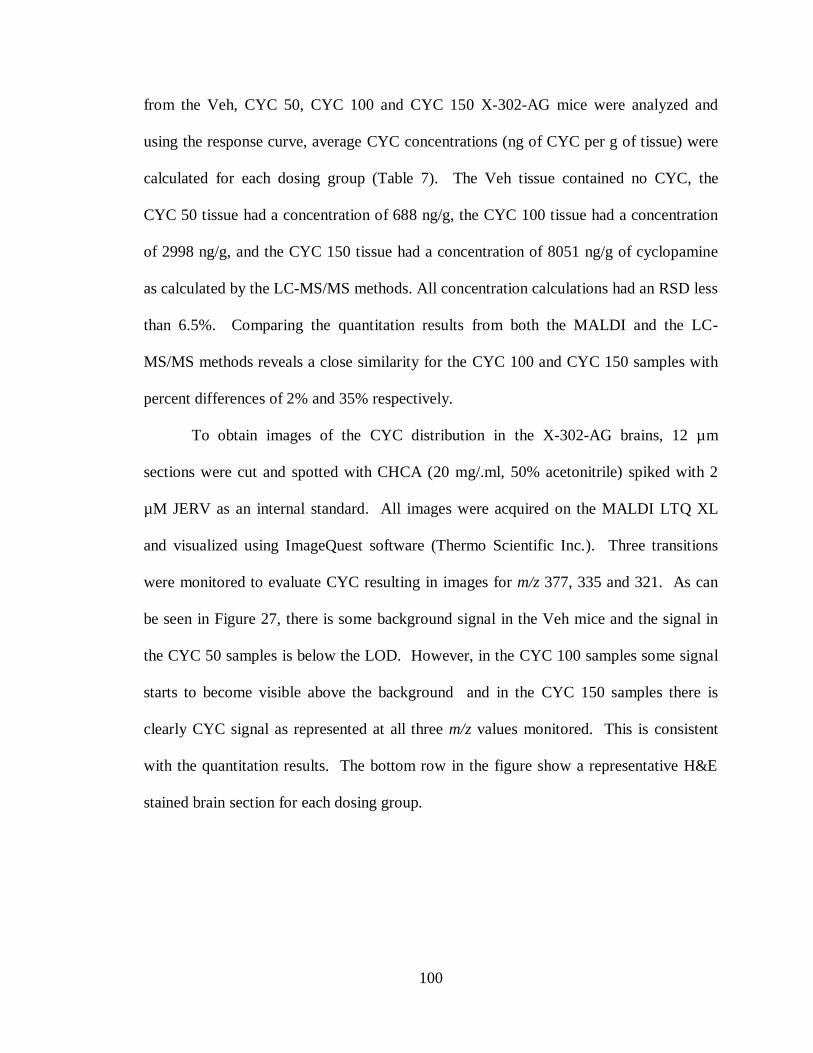
100

from the Veh, CYC 50, CYC 100 and CYC 150 X-302-AG mice were analyzed and

using the response curve, average CYC concentrations (ng of CYC per g of tissue) were

calculated for each dosing group (Table 7). The Veh tissue contained no CYC, the

CYC 50 tissue had a concentration of 688 ng/g, the CYC 100 tissue had a concentration

of 2998 ng/g, and the CYC 150 tissue had a concentration of 8051 ng/g of cyclopamine

as calculated by the LC-MS/MS methods. All concentration calculations had an RSD less

than 6.5%. Comparing the quantitation results from both the MALDI and the LC-

MS/MS methods reveals a close similarity for the CYC 100 and CYC 150 samples with

percent differences of 2% and 35% respectively.

To obtain images of the CYC distribution in the X-302-AG brains, 12 µm

sections were cut and spotted with CHCA (20 mg/.ml, 50% acetonitrile) spiked with 2

µM JERV as an internal standard. All images were acquired on the MALDI LTQ XL

and visualized using ImageQuest software (Thermo Scientific Inc.). Three transitions

were monitored to evaluate CYC resulting in images for m/z 377, 335 and 321. As can

be seen in Figure 27, there is some background signal in the Veh mice and the signal in

the CYC 50 samples is below the LOD. However, in the CYC 100 samples some signal

starts to become visible above the background and in the CYC 150 samples there is

clearly CYC signal as represented at all three m/z values monitored. This is consistent

with the quantitation results. The bottom row in the figure show a representative H&E

stained brain section for each dosing group.

101

Figure 27: Images of cyclopamine distribution in the dosed X-302-AG brain sections at

each dosing level. m/z values 377, 335 and 321 were monitored. Background signal can

be seen in the Veh brains and the signal in the 50mg/kg/day dosed brains is below the

LOD. Some signal is visible above the LOD in the 100 mg/kg/day brains and there is

distinct CYC signal in the 150 mg/kg/day samples. The bottom row shows a

representative H&E stained brain section for each dosing group.

Responder versus Non-Responder Proteome Study

In a study parallel to this one, the operational status of the Hh pathway in the

malignant glioma specimens used for the xenografts was determined. Gliomaspheres

(GS) were generated for two of the three specimens (GS-312-HGA and GS-406-GBM)

under culture conditions required for eliciting a Hh pathway response in glioma primary

cell cultures.130

It was found that an operational Hh pathway was present in the 312-

102

HGA primary tumors but that the 406-GBM tumor lacks an operational Hh pathway. In

order to determine the effect of in vivo Hh pathway inhibition by cyclopamine X-312-

HGA and X-406-GBM mice were treated and assayed for survival. It was found that

continuous treatment with CYC (50mg/kg twice daily) showed a median survival

difference of 11.5 days (P=0.0062, Logrank test) in X-312-HGA mice but no difference

in survival was measured in the X-406-GBM mice receiving the same CYC treatment

(Figure 28).130

Figure 28: Hedgehog pathway inhibition confers a survival advantage. A) Treatment

was initiated in X-312-HGA mice 50 days after xenotransplantation and continued for the

duration of the survival study. Cyclopamine-treated mice (50 mg/kg twice daily) had a

median survival of 11.5 days longer than vehicle-treated mice (P =0.0062, Logrank test).

B) Continuous cyclopamine treatment of X-406-GBM mice (50 mg/kg twice daily

starting 100 days after xenotransplantation) did not enhance survival (P =0.56, Logrank

test). Solid grey bars indicate duration of treatment. (Figure adapted from A. Sarangi

et.al)130

103

To further investigate the differences between the CYC responder (X-312-HGA)

and non-responder (X-406-GBM) xenografts, protein images were taken from the brains

using MALDI TOF IMS. Standard MALDI imaging preparation techniques were

employed to get the samples ready for analysis. The CYC treated and control brains were

cut on a cryostat and sections were thaw mounted onto target slides, dried and then

matrix was applied using a Portrait™ 630 spotter before imaging on a Bruker Autoflex

TOF MS. Three sections were analyzed for each brain and sample acquisition was

randomized to eliminate bias. Serial sections were cut for each brain and stained with

anti-human nuclear immunohistochemistry. The stained sections were scanned on a

Mirax Scanner (Carl Zeiss MicroImaging) and the images were saved. All sections were

evaluated by a trained neuropathologist to mark areas of tumor invaded and non-invaded

regions. Eight regions were marked using the Mirax software; striatum, invaded

striatum, lateral ventricle (LV), invaded lateral ventricle, grey matter, invaded grey

matter, corpus collosum (CC) and invaded corpus collosum (Figure 29). The X-406-

GBM brains were so infiltrated with tumor cells that there was no non-invaded tissue to

be marked by the pathologist and there was no invaded grey region in the X-312-HGA

samples.

After acquisition of the MALDI images, it was then possible to co-register and

overlay the marked brain images using Flex Imaging software (Bruker Daltonics). These

overlays allowed for the visualization of all the MALDI images and align which spectra

came from within the specific regions of brain tissue marked by the neuropathologist.

The spectra were then selected, choosing approximately ten spectra per region for each

104

Figure 29: Anti-human nuclear stained brain tissue section from a primary tumor

xenograft (X-312-HGA). The section was scanned on a Mirax scanner and then various

histological regions were marked by a neuropathologist. Each color represents a different

area of the brain: grey matter (grey), invaded grey matter (orange), corpus collosum

(pink), invaded corpus collosum (yellow), striatum (green), invaded striatum (red), lateral

ventricle (purple) and invaded lateral ventricle (teal).

brain section analyzed, and placed in separate folders for further processing and statistical

analysis.

All spectra were processed using ClinPro Tools, commercially available software

from Bruker Daltonics. Once the spectra had undergone baseline subtraction, smoothing,

normalization, realignment and peak picking, the data for each spectrum was exported

collectively into a feature table, which is a list of each m/z value and its corresponding

intensity value for each spectrum. The mass region evaluated was from m/z 3000-30,000

and there was an average of 240 peaks found for each brain region. Using these feature

105

tables, various analyses and statistical tests were performed to evaluate the protein

changes that occurred with respect to the cyclopamine treatment.

Comparisons were made for each area of the brain, comparing CYC dosed versus

non-dosed samples for both the X-312-HGA and X-406-GBM mouse brains. SAM

analysis was performed for each region and resulted in lists of m/z values that show a

significant difference between the dosed and non-dosed brains. The SAM used a two

class unpaired test and significant peaks were identified that had a fold change > 1.25.

There were a number of peaks that were changed as a result of the CYC treatment. For

the X-312-HGA samples, the invaded CC had 49 (21%), the invaded LV had 121 (48%)

and the invaded striatum had 61 (25%) significant peak changes (Table 8). For the X-

406-GBM samples, the invaded CC had 54 (23%), the invaded grey had 54 (22%), the

invaded LV had 91 (36%) and the invaded striatum had 99 (41%) significant peak

changes (Table 8).

Table 8: Significant peak change statistics for the X-312-HGA and X-406-GBM

xenograft mice.

NonDosed Versus Dosed

Fold Change > 1.25 X-312-HGA X-406-GBM

Total #

Peaks

#

Affected

Peaks

% of

peaks

changed

FDR* #

Affected

Peaks

% of

peaks

changed

FDR*

Invaded CC 234 49 21 16.5 54 23 5.2

Invaded Grey 247 N/A N/A N/A 54 22 12.1

Invaded LV 254 121 48 22.1 91 36 22.7

Invaded Striatum 244 61 25 14.3 99 41 1.6

CC 230 144 63 9.7 N/A N/A N/A

Grey 257 32 12 11.7 N/A N/A N/A

LV 229 79 34 26.5 N/A N/A N/A

Striatum 228 51 22 8.7 N/A N/A N/A

*FDR- False Discovery Rate

106

There are various ways to look at the significant peak changes when comparing

the X-312-HGA (CYC responsive) and X-406-GBM (CYC non-response) xenografts.

Appendix B shows that there are some significant features that go up in both xenografts

and some that go down in both xenografts. There are also some significant features that

go up in one xenograft and down in the other and there are unique significant features to

each xenograft. An example of this is displayed in Figure 30 which shows a graphical

representation showing the percent change for each m/z in a signature of response found

for the X-312-HGA responder xenograft tumors in the invaded striatum region. The

signals are arranged from greatest negative percent change to greatest positive percent

change in the responder profiles. The X-406-GBM non-responder graph displays the

same order of features, showing that the majority of the signals do not display a

significant change in intensity and some features display an opposite response to the

CYC than the X-312-HGA tissues.

Protein identifications were found for 40 of the significant features that were

affected by cyclopamine dosing in the X-312-HGA xenografts which showed a survival

advantage as a result of treatment. Protein identification was achieved through protein

separation/isolation, proteolytic digestion, sequencing of peptides by LC-MS/MS, and

matching the peptides to genome-based protein databases. The MALDI peaks identified

using these strategies are shown in Table 9. The MW and corresponding identifications

are listed along with the percent coverage, modifications, SwissProt Identification

number, the number of peptides identified, the intensity trend as a result of CYC dosing

and the regions in the brain the features were found.

107

Figure 30: SAM results displayed as bar graphs for the Invaded Striatum of the

xenografts comparing CYC dosed versus non-dosed tissues. In the top graph each bar

represents the percent change for each m/z in a signature of response found for the X-12-

HGG responder xenograft tumors. The signals are arranged from greatest negative

percent change to greatest positive percent change in the responder profiles. The bottom

graph displays the same order of features as the top graph, with each bar representing the

percent change for each m/z in the X-406-GBM samples. The majority of the signals do

not display a significant change in intensity, however, some m/z signals display an

opposite trend between the responder and non-responder samples. Spectra used in the

comparison of treated to non-treated were isolated from the tumor invaded striatum of the

brains, as determined by a neuropathologist. Before SAM analysis the spectra were

processed (baseline-subtracted, smoothed, normalized and re-aligned).

108

Table 9: Protein Identifications for Significant Features in the X-312-HGA xenografts

(CYC responsive)

*acetylated N-terminus (+42)

^opposite trend seen in X-406-GBM xenograft samples

m/z MW (Da) Protein Name

% Coverage

of

unprocessed

precursor

Modifications

(amino acid

chain)

Swissprot

Primary

Accession

Number

Number

of

Peptides Trend Brain Region

6722 6807 Purkinje cell protein 4 39 *(2-62) P63054 2 Down^

Invaded Striatum

Invaded LV

7342 7338 Copper transport

protein ATOX1 44 (1-68) O08997 3 Down^

Invaded Striatum

Invaded LV

7359 7446 Cytochrome b-c1

complex subunit 9 34 *(2-64) Q8R1I1 2 Down^

Invaded Striatum

Invaded LV

7543 7498 Myelin basic protein

(Isoform 3) 41 *(1-69) P04370 5 Down

Invaded Striatum

Invaded LV

7960 7960

cAMP-dependent

protein kinase inhibitor

alpha 48 (1-76) P63248 2 Down^ Invaded LV

8026 7979

Guanine nucleotide-

binding protein

G(I)/G(S)/G(O) subunit

gamma-13 13 *(1-67) Q9JMF3 2 Up Invaded CC

8110 8236 ATP synthase subunit

e, mitochondrial 51 (2-71) Q06185 6 Down

Invaded Striatum

Invaded LV

8675 8761 Probable protein

BRICK1 29 *(2-75) Q91VR8 2 Down Invaded LV

9330 9327

NADH dehydrogenase

[ubiquinone] 1 alpha

subcomplex subunit 4 43 (2-82) Q62425 4 Down^

Invaded Striatum

Invaded LV

9639 9768 Cytochrome b-c1

complex subunit 8 54 (2-82) Q9CQ69 3 Down^

Invaded Striatum

Invaded LV

9980 10071 Cytochrome c oxidase

subunit 6B1 38 *(2-86) P56391 4 Down Invaded LV

10522 10477

SH3 domain-binding

glutamic acid-rich-like

protein 3 25 *(1-93) Q91VW3 2 Up

Invaded Striatum

Invaded LV

10724 10855

LYR motif-containing

protein 4 34 (2-91) Q8K215 3 Up Invaded CC

10834 10963 Heat shock protein 1

(Chaperonin 10) 57 (2-102) Q4KL76 6 Up^ Invaded Striatum

11086 11083 Protein S100-A11 16 (1-98) P50543 2 Down Invaded LV

11517 11605 Cytochrome c, somatic 32 *(2-105) P62897 5 Up

Invaded Striatum

Invaded LV

11652 11651 60S acidic ribosomal

protein P2 66 (1-115) P99027 4 Up^

Invaded Striatum

Invaded LV

11545 11675 Thioredoxin 38 *(2-105) P10639 4 Up

Invaded Striatum

Invaded LV

11799 11923

Peptidyl-prolyl cis-

trans isomerase

FKBP1A 43 (2-108) P26883 3 Down Invaded LV

12137 12136

Tumor suppressor

candidate 2 32 (1-110) Q9WVF8 2 Down^

Invaded Striatum

Invaded LV

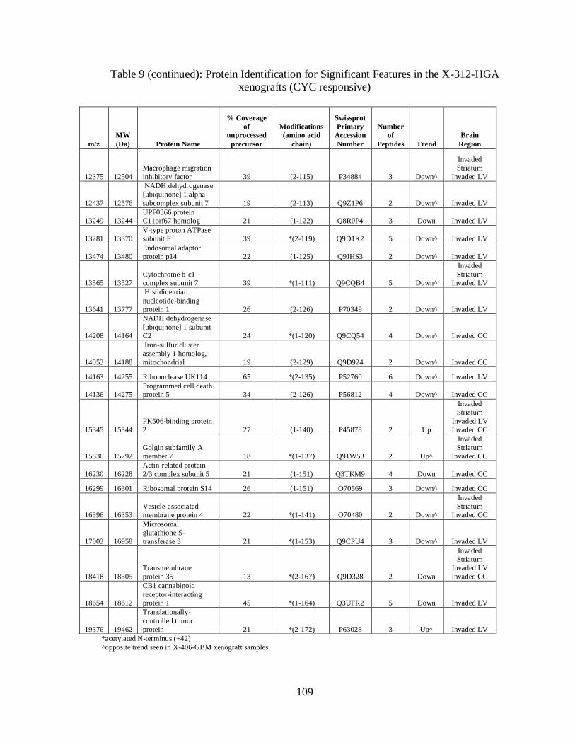
109

Table 9 (continued): Protein Identification for Significant Features in the X-312-HGA

xenografts (CYC responsive)

*acetylated N-terminus (+42)

^opposite trend seen in X-406-GBM xenograft samples

m/z

MW

(Da) Protein Name

% Coverage

of

unprocessed

precursor

Modifications

(amino acid

chain)

Swissprot

Primary

Accession

Number

Number

of

Peptides Trend

Brain

Region

12375 12504

Macrophage migration

inhibitory factor 39 (2-115) P34884 3 Down^

Invaded

Striatum

Invaded LV

12437 12576

NADH dehydrogenase

[ubiquinone] 1 alpha

subcomplex subunit 7 19 (2-113) Q9Z1P6 2 Down^ Invaded LV

13249 13244

UPF0366 protein

C11orf67 homolog 21 (1-122) Q8R0P4 3 Down Invaded LV

13281 13370

V-type proton ATPase

subunit F 39 *(2-119) Q9D1K2 5 Down^ Invaded LV

13474 13480

Endosomal adaptor

protein p14 22 (1-125) Q9JHS3 2 Down^ Invaded LV

13565 13527

Cytochrome b-c1

complex subunit 7 39 *(1-111) Q9CQB4 5 Down^

Invaded

Striatum

Invaded LV

13641 13777

Histidine triad

nucleotide-binding

protein 1 26 (2-126) P70349 2 Down^ Invaded LV

14208 14164

NADH dehydrogenase

[ubiquinone] 1 subunit

C2 24 *(1-120) Q9CQ54 4 Down^ Invaded CC

14053 14188

Iron-sulfur cluster

assembly 1 homolog,

mitochondrial 19 (2-129) Q9D924 2 Down^ Invaded CC

14163 14255 Ribonuclease UK114 65 *(2-135) P52760 6 Down^ Invaded LV

14136 14275

Programmed cell death

protein 5 34 (2-126) P56812 4 Down^ Invaded CC

15345 15344

FK506-binding protein

2 27 (1-140) P45878 2 Up

Invaded

Striatum

Invaded LV

Invaded CC

15836 15792

Golgin subfamily A

member 7 18 *(1-137) Q91W53 2 Up^

Invaded

Striatum

Invaded CC

16230 16228

Actin-related protein

2/3 complex subunit 5 21 (1-151) Q3TKM9 4 Down Invaded CC

16299 16301 Ribosomal protein S14 26 (1-151) O70569 3 Down^ Invaded CC

16396 16353

Vesicle-associated

membrane protein 4 22 *(1-141) O70480 2 Down^

Invaded

Striatum

Invaded CC

17003 16958

Microsomal

glutathione S-

transferase 3 21 *(1-153) Q9CPU4 3 Down^ Invaded LV

18418 18505

Transmembrane

protein 35 13 *(2-167) Q9D328 2 Down

Invaded

Striatum

Invaded LV

Invaded CC

18654 18612

CB1 cannabinoid

receptor-interacting

protein 1 45 *(1-164) Q3UFR2 5 Down Invaded LV

19376 19462

Translationally-

controlled tumor

protein 21 *(2-172) P63028 3 Up^ Invaded LV

110

Discussion

Most previously reported methodologies for CYC quantitation involved

the use of LC-MS/MS and was shown for concentration in plasma and cultured cells.

This study extends on that work to include a methodology to quantify CYC in tissues

while maintaining spatial integrity using MALDI and demonstrates for the first time the

concentration of CYC in brain tumor xenografts (Table 7). Comparing the concentration

values found by the MALDI with the LC-MS/MS method developed for CYC

quantitation from tissue shows close similarity. The percent difference in the samples

was approximately 35% for the CYC 150 samples and was only 2% for the CYC100

samples. The CYC 50 and Veh samples had CYC concentration below the LOD for the

MALDI method and with the LC-MS/MS the CYC 50 cyclopamine concentration was

only determined to be 688 ng/g. The low concentration could be due to the fact that the

half life of the CYC has been shown to be 4h and the samples were taken 5h post dose. It

has been shown that administration of cyclopamine by ip injection caused minimal

toxicity at doses of 10 mg/kg and 50 mg/kg while a high dose tested (160 mg/kg)

demonstrated toxicity.142

This study also showed maximum serum concentration (Cmax)

was reached 20 min (Tmax) following injection of 10 or 50 mg/kg doses with

corresponding Cmax values of 2.58 and 19.9μM, respectively. The terminal elimination

half-life of cyclopamine administered ip was 4h.142

Cyclopamine has been shown to inhibit the Shh pathway in brain tumor

xenografts and confers a survival advantage.130

By studying the proteomic affects of the

CYC dosing on these xenografts, it is possible to see what affects related to the Shh

111

pathway are seen as well as point to other possible biological pathways that are affected.

Statistical analysis found numerous protein signals that were affected by the cyclopamine

treatment in both the responder X-312-HGA and non-responder X-406-GBM xenografts

(Table 8). By focusing on the signals that were altered in the responder xenograft (Table

9), it can help shed insight into how the CYC is inhibiting tumor growth and increasing

survival.

Purkinje cell protein 4 was decreased in the CYC dosed X-312-HGA xenograft

mice. Shh is produced by Purkinje cells from late embryonic stages of development

through to adulthood. The loss of Shh activity influences Purkinje cell development.143

The inhibition of the Shh pathway would thus affect the expression of the purkinje cell

proteins.

Endosomal adaptor protein p14 was found to have a decreased intensity in the

treated X-312-HGA samples as compared to the non-treated samples. Endosomal

adaptor protein p14 is a regulator of the mTOR pathway, a signaling cascade that

regulates both cell growth and cell cycle progression through its ability to integrate

signals from amino acids and energy.144

As part of the Ragulator complex, it recruits the

Rag GTPases and the mTORC1 complex to lysosomes, a necessary key step in activation

of the TOR signaling cascade by amino acids.145

The antiproliferative effects of mTOR

inhibition has been observed in multiple cancerous cell lines also including inhibition of

protein synthesis and induction of apoptosis. The decrease in intensity of the endosomal

adaptor protein p14 in the responder xenograft could indicate that cyclopamine serves to

inhibit the mTOR pathway and this could be another way that cyclopamine inhibits cell

proliferation and reduces tumor size in addition to its Hh inhibiting properties.146

112

Treatment with CYC in the X-312-HGA drug responsive xenograft shows a

decrease in S100A11 (Calgizzarin), which is a calcium-binding protein implicated in a

variety of biologic functions such as cytoskeleton organization, proliferation and

differentiation. Overexpression of S100A11 has been shown in a number of cancers such

as prostate,147

colorectal,148

pancreatic,149

and breast150

suggesting that it may be involved

with cancer development and progression. It has been demonstrated that suppression of

S100A11 by small interfering RNA (siRNA) led to apoptosis, and that the overexpression

of S100A11 inhibited apoptosis in human uterine smooth muscle tumor cells.151

The

proapoptotic effect of calgizzarin downregulation was also shown with TSA treatments

antitumoral effect suggested by another study.152

This indicates that the CYC treatment

could be inducing apoptotic pathways in the drug responsive xenografts.

Numerous proteins involved in the electron transport chain were affected by

cyclopamine treatment in the X-312-HGA CYC responder xenografts. NADH

dehydrogenase [ubiquinone] 1 alpha subcomplex subunit 4 along with subcomplex

subunits 4 and 7 are all a part of Complex I. Cytochrome b-c1 complex subunits 7,8 and

9 are a part of Complex III, cytochrome c oxidase subunit 6B1 is a part of Complex IV

and ATP synthase subunit 3 is part of Complex V. All of the above mentioned proteins

showed a decrease in intensity in the X-312-HGA CYC treated xenografts versus the

non-treated xenograft samples. Cytochrome c, however, showed an increase in intensity.

As described in Chapter III, the electron transport chain, which is embedded in

the inner membrane of the mitochondria, consists of five multi-protein complexes.

Complexes I and II oxidize the energy-rich molecules NADH and FADH2, respectively,

and transfer the resulting electrons to ubiquinol, which carries it to complex III. Complex

113

III, in turn, shuttles the electrons across the inner mitochondrial membrane to cytochrome

c, which carries them to complex IV. Complex IV uses the electrons to reduce oxygen to

water. Each electron carrying step uses the resulting energy to pump hydrogen ions into

the intermembrane space. This generates a proton gradient, the dissipation of which is

used by complex V, or ATPase, to power the phosphorylation of ADP to ATP. Along

with carrying electrons, complexes I, II, and III generate reactive oxygen species (ROS),

namely superoxide, at low levels.153

By inhibiting the electron transport chain, there is a greater generation of ROS

which occurs at the tumor mitochondrial membrane.154

This activates apoptosis by

facilitating the release of cytochrome c from the inner mitochondrial membrane. Bcl-2

proteins are layered on the surface of the mitochondria, detect damage, and activate a

class of proteins called Bax, which punch holes in the mitochondrial membrane, causing

cytochrome c to leak out. This cytochrome c binds to Apaf-1, or apoptotic protease

activating factor-1, which is free-floating in the cell‟s cytoplasm. Using energy from the

ATPs in the mitochondrion, the Apaf-1 and cytochrome c bind together to form

apoptosomes. The apoptosomes bind to and activate caspase-9, another free-floating

protein. The caspase-9 then cleaves the proteins of the mitochondrial membrane, causing

it to break down and start a chain reaction of protein denaturation and eventually

phagocytosis of the cell.155

Numerous studies have shown that by inhibiting the complexes of the

mitochondrial electron transport chain (most documented for Complex I and III) there is

an increase in ROS production and subsequent cell death.156-158

Recently, several studies

have also indicated that ROS may be also involved in induction of autophagy.159, 160

114

Autophagy is a self-digestion process important for cell survival during starvation. It has

also been described as a form of programmed cell death. Mitochondria are important

regulators of autophagy-induced cell death and damaged mitochondria are often degraded

by autophagosomes. The decrease in the ETC complex proteins indicates that CYC is

suppressing the ETC system which could be resulting in increased ROS production. This

ROS increase is most likely facilitating the increase in cytochrome c and subsequent

apoptotic mechanisms.

As is evidenced, a number of vital biological processes were affected by the

administration of CYC in the X-312-HGA xenografts including ETC function, the mTOR

pathway and apoptosis mechanisms. Most of the effects were seen in multiple regions of

the invaded brain indicating that the CYC administration has a ubiquitous effect on the

tumor cells regardless of their location. Further work is needed to identify all of the

molecular features that were altered and fully elucidate what this could mean biologically

as well as validate the proteins as viable markers of CYC efficacy. Additional evaluation

should also be done to investigate the molecular features that were affected solely in the

X-406-GBM samples. These changes could be indicative of affects that are nonspecific

to the CYC tumor reducing activity.

MALDI IMS has shown to be a very powerful discovery technique for

investigating the molecular effects that cyclopamine administration has in direct human

glioma xenografts. The data provides not only information as to the pharmacological

response of the CYC but also provides a means to directly correlate drug distribution with

these molecular changes and obtain drug concentration information all while maintaining

spatial information in the tissue samples.

115

Materials and Methods

Materials

The MALDI matrices, sinapinic acid and 2,5-dihydroxybenzoic acid,

hemotoxylin, cyclopamine, and jervine, normal horse serum, mouse raised anti-human

primary antibody, horse raised anti-mouse secondary antibody, DAB solution and DAB

buffer, and Avidin and Biotin and Avidin HRP were purchased from Sigma Chemical

Co. (St. Louis, MO). Acetic acid, HPLC grade acetonitrile, ethanol, and methanol,

Xylene, Para formaldehyde, Triton X100, PBS and Hydrogen Peroxide were purchased

from Fisher Scientific (Suwanee, GA).

Tissue Preparation and MALDI Imaging

Tissue was obtained from Dr. Michael Cooper‟s laboratory (Vanderbilt

University, Nashville, TN). CD133-enriched cells (104–10

5) were transplanted into the

striatum of NOD/SCID mice according to a protocol approved by the Vanderbilt Medical

Center IACUC. Mice were anesthetized with ketamine and xylazine, and securely placed

on a stereotactic frame. Using aseptic surgical procedures, an incision was made in the

scalp and a small burr hole was drilled 2.5 mm lateral to the bregma. CD133-enriched

cells were implanted 2.5 mm into the right striatum using a Hamilton syringe. Mice were

maintained until development of neurological symptoms or signs of distress.130

After

sacrifice the brains were removed and a sagittal section at Interaural 10.6 mm, Bregma

1.6 mm was cut and flash frozen in liquid nitrogen and stored at -80 °C until further use.

116

Frozen brain tissues were mounted onto a cryostat chuck with OTC. Tissue was

trimmed until an even sagittal section was acquired. From this position sections (12 µm)

were collected, one for protein analysis, a serial section for CYC analysis, and another

serial section for anti-human nuclear immunohistochemical staining. Sections for protein

and CYC analysis were mounted onto gold-coated MALDI targets while the sections for

staining were thaw mounted onto glass microscope slides.

Slides were immediately stained, or stored at -20 °C until staining. Slides were

put into 4% Paraformaldehyde for 60 minutes at 4 °C before being removed and dried for

two minutes at room temperature. Slides were then put into 1x PBS for five minutes then

quenched with 1% hydrogen peroxide for 20 minutes. The slides were washed in

phosphate buffer solution with triton X (PBST) twice for five minutes before adding a

normal blocking horse serum (10% in 0.1% PBST) for 30 minutes. Again the slides were

washed in PBST twice for five minutes each wash. An avidin biotin block was done, the

slides were washed in PBST before the antibodies were applied. Primary antibody

(mouse raised, anti-human) was applied for 8-12 hours at 4 °C, slides were washed in

PBST then secondary antibody (horse raised, anti-mouse) was added for two hours at

room temperature. Again the slides were washed in PBST. Avidin/HRP was added for

one hour, slides were washed in PBST then DAB was added in the dark for 8 minutes.

The slides were briefly dipped in water and then Hemotoxylin counterstained before

undergoing a series of ethanol washes to dehydrate the slides before rinsing in xylene and

then coverslipping.

MALDI targets were placed into a desiccator for at least an hour to dry. To

prepare sections for CYC analysis, a matrix solution of CHCA (20 mg/ml, 50%

117

acetonitrile) was prepared with 2 µM JERV internal standard. Sections were spotted on

the Portrait (Flyby 1 drop 20 passes x2) at 300 µm x 300 µm spatial resolution. All CYC

images were acquired on a MALDI-LTQ XL (Thermo Scientific Inc.). The MALDI

target with sections designated for protein analysis was reagent washed and seeded with

finely ground SA. Fresh SA matrix solution was made 60% acetonitrile 40% water

0.02% TFA. The sections were spotted using the Portrait (Flyby 1 drop 30 repeats) in a

300 µm x 300 µm array. Higher spatial resolution images were spotted at 150 µm x 150

µm. The MALDI target was scanned and sections were imaged on an Autoflex (Bruker

Daltoniks).

The immunohistochemically stained sections stained were scanned on a Mirax

Scanner and .jpeg images were exported. Histological markings were made by a trained

neuropathologist (Tye Able) using Mirax Software (Carl Zeiss International). Eight

regions were marked, striatum, invaded striatum, lateral ventricle, invaded lateral

ventricle, grey matter, invaded grey matter, corpus collosum and invaded corpus

collosum. The marked images were then co-registered with the images acquired to

extract spectra from isolated histological areas for comparisons and further statistics.

Data Processing

Spectra from each section were kept together in separate folders. These folders

were then input into ClinPro Tools where the imported spectra were processed with the

following parameters; 1200 Resolution, data reduction factor of 5, Top Hat baselining

with 10% Minimal Baseline Width, Savitsky Golay Smoothing enabled at 2 width 10

cycles, recalibration 2000 ppm max peak shift with 20% match to calibrate peaks

118

excluded not re-calibratable spectra, from m/z range 3000-20,000, and null spectra

exclusion. Once Spectra have been imported into ClinPro Tools and processed peak

selection was performed (peak picking on total average spectrum, SN=2, 0% relative

threshold to the base peak) and peak list feature tables were output.

Statistical Analysis

SAM was performed to assign a score to each feature on the basis of change in its

spectral intensity relative to the standard deviation of repeated measurements. For

features with a score greater than a predetermined threshold, SAM uses permutations of

the repeated measurements to estimate the percentage of features identified by chance,

the false discovery rate 91

. Two by two comparisons were made for each brain region

comparing dosed versus non-dosed tissue sections. Both the X-312-HGA (responder)

and X-406-GBM (non-responder) xenograft spectra were analyzed.

Drug Quantitation Using LC-MS/MS

The extraction and chromatographic LC-MS/MS protocols used here for were

adapted from previous methodologies used for CYC quantitation.142, 161-163

Cyclopamine

and jervine stock solutions were made in MeOH and stored at -20 °C until use.

Calibration curves standards were made in control mouse brain homogenate to yield final

concentrations of 1000, 100, 10, 1, 0.1, 0.01 ng/ml of CYC. A minimum of 20 mg of

tissue was weighed out for sample analysis. The tissue was homogenized with PBS in a

10:1 (ml/mg) ratio until uniform upon visual inspection. The homogenate was sonicated

for ten minutes and then centrifuged at 3500 g for 15 minutes and then 4000 g for 15

119

minutes. Fifty µl of the supernatant was taken and mixed with 25 µl of internal standard

(jervine, 1000 ng/ml). For protein precipitation, 250 µl of acetonitrile /ethanol/acetic acid

(90/10/0.1) was added and vortex mixed for 20 minutes. The solution was then

centrifuged for 15 minutes at 4000 g. Supernatant was transferred to a glass autosampler

tube and dried in a vacuum centrifuge (two hours, 40 °C) and then reconstituted in 50%

methanol with 0.1% formic acid.

Samples were analyzed on an ESI TSQ Quantum triple-quadrupole system

(Thermo Scientific, Waltham, MA) equipped with an autosampler (set at 4 ºC) column

oven (50 °C) and HPLC system. A Waters XTerra RP® C18 reverse phase column (2.1 x

100 mm, 5 µm particle) was used with a fast gradient run of mobile phase A (0.1% acetic

acid in water) to mobile phase B (0.1% acetic acid in methanol). Ten microliters of

sample was injected onto a PEEK loop at a flow rate of 0.3 ml/min at 5% mobile phase B

and held for one minute. Over 5 minutes a linear gradient was run from 5%-95% mobile

phase B and then held at 95% for one minute. The column was then eluted from 95%-5%

over one minute and then held at 5% mobile phase B for two minutes before injection of

the next sample. The total run time was ten minutes.

Acknowledgements

Dr. Annurag Sarangi and Dr. Michael Cooper performed the mouse implantation

and dosing with cyclopamine. All mice samples and survival study data provided by Dr.

Michael Cooper‟s Lab. All histological markings were made by Dr. Tye Able.

120

CHAPTER V

CONCLUSIONS AND PERSPECTIVES

The Value of MALDI Imaging in Drug Discovery and Development

Despite the dramatic increase in drug development expenditures over the last

decade, the number of new chemical entities has actually decreased. The industry has

been troubled by high late-stage attrition rates and safety issues, creating a major problem

not only for drug developers, but also for regulatory agencies, patients, and society in

general. Current methodologies involved with drug discovery and development are

clearly in need of assistance. New approaches and new science are needed to transform

drug development.

It has been shown that MS plays a role in all aspects of the drug discovery and

development process. Current mass spectrometry technologies are applied in ADME

screening for lead compound optimization, drug quantification in PK studies, drug

metabolite identification in animals and humans, as well as PD bioanalysis in both

clinical and toxicology studies.164

The technology's value spans the entire drug pipeline.

It has been said that MS has become almost a cornerstone of modern drug discovery and

development, from target identification and validation up to combinatorial chemistry and

parallel synthesis chemistry. MS is seen in everything from new chemical entities to

formula determination to target profiling and preclinical studies. It is even seen at the far

end, in manufacturing and many researchers are working to bring mass spectrometry into

diagnostics.10, 164

121

Throughout the course of this research it has been demonstrated how MALDI

IMS can extend the use of MS in drug discovery and development even further by

introducing a new method for sample analysis. A MALDI IMS protocol was developed

for absolute quantitation of small molecules directly from tissue sections (Chapter II).

This protocol allows for MALDI based imaging technologies to correlate absolute drug

concentration with pharmacological response in tissues while still maintaining spatial

information in rapid, high-throughput molecularly specific experiments as demonstrated

in Chapters III and IV.

Imaging experiments performed by MALDI were able to provide the individual,

label-free temporal distributions of OLZ, IMAT and CYC from brain tissue sections with

high sensitivity and reproducibility. Highly-accurate absolute quantities of each

compound were also obtained directly from tissue sections without the need for

homogenization or extraction procedures. This proves advantageous over LC-MS/MS

techniques in that spatial information is retained, sample preparation as well as sample

analysis is quicker and there is less chance of losing quantities of the small molecule

being investigated during the preparation or analysis processes. The use of this

technology could be implemented in early phases of pre-clinical trials to assist with PK

studies in animal models.

Using the calculated drug concentrations of IMAT and CYC, it was possible to

study the proteome affects that the drug presence had on primary brain tumor xenografts

in mice. With the ultimate goal of PD studies being to relate the pharmacological

response to dose-concentration or concentration-effect relationships of a therapeutic

compound, MALDI IMS proved to be an invaluable tool to rapidly and reproducibly

122

relate the tissue distribution of the IMAT and CYC to the observed pharmacological

response within the same tissue sample while maintaining spatial resolution.

Altered proteins were identified that are involved in a number of different

biological pathways, such as the ETC, apoptosis mechanisms, proliferation, cell cycle

regulation and pre-mRNA splicing. Future studies about the biological implications of

the perturbation in expression of these proteins may also facilitate the discovery of

additional molecular pathways that are altered by IMAT and CYC in primary brain

tumors. This may contribute to an improved understanding of the IMAT and CYC

mechanisms of action within the tumors or provide new possible drug targets for the

development of additional therapies. Taken together, the pharmacoproteomic profiling

could constitute a valuable tool for the identification of drug-responsive biomarkers and

for the establishment of a molecular basis for developing novel and more effective

approaches for therapeutic intervention. The biological information obtained could also

help gain a deeper understanding of the mechanisms involved in primary brain tumor

function.

Future Research Directions

As is important to all new technologic methods to be used in clinical research,

issues related to quality control, standardization, specimen choice and collection, result

interpretation and validation all need to be taken into consideration. Publication is only

the first step in acceptance and utilization of a new approach. A key hurdle in this

process is the ability to bridge the pre-clinical trials into a positive clinical trial outcome.

123

With the push towards personalized medicine, the requirement for accurate

molecular diagnostics for the characterization of human disease to deliver the most

effective therapies is driving research towards developing more and novel biomarkers.165

Typical approaches towards the discovery and validation of these biomarkers involve

initial studies in vitro, followed by in vivo studies with small animal molecules before

progressing to clinical studies in humans.165

MALDI IMS technologies and methods

have become key in the discovery and utilization of biomarkers for disease diagnosis,

prognosis and compound efficacy determination that are relevant to human disease.

Pairing the analysis of mouse model samples with patient samples of the same

disease will improve the ability to find viable and accurate biomarkers. As described in

Chapter IV, the mouse xenografts used were developed directly from patient biopsy

samples. Recapitulation of the malignant glioma pathological features was observed and

gliomaspheres generated from the tissues demonstrated active biological activity that was

also seen in the xenograft models130

This shows that the xenografts are very good

representations of the brain tumor diseases that were present in the patients.

MALDI IMS techniques were used to analyze sections of the patient biopsies that

were used to develop the xenografts. Frozen biopsy tissues were sectioned on a cryostat

at 12 µm, mounted onto target slides, washed, dried, spotted using the Portrait with SA

and analyzed using a MALDI TOF. Images were visualized using Flex Imaging software

(Bruker Daltoniks). Significant features found in the xenografts (Chapter IV) were

looked for in the biopsy samples. Multiple signals were found that corresponded to both

a CYC response in the xenograft mice and presence in the patient biopsies. As is seen in

Figure 31, the m/z signal 7008 is visualized in the xenograft tissue sections as well as the

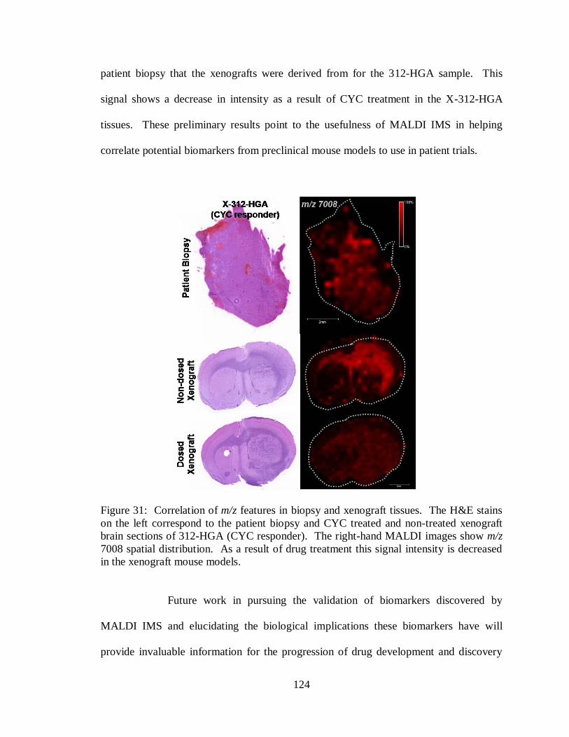
124

patient biopsy that the xenografts were derived from for the 312-HGA sample. This

signal shows a decrease in intensity as a result of CYC treatment in the X-312-HGA

tissues. These preliminary results point to the usefulness of MALDI IMS in helping

correlate potential biomarkers from preclinical mouse models to use in patient trials.

Figure 31: Correlation of m/z features in biopsy and xenograft tissues. The H&E stains

on the left correspond to the patient biopsy and CYC treated and non-treated xenograft

brain sections of 312-HGA (CYC responder). The right-hand MALDI images show m/z

7008 spatial distribution. As a result of drug treatment this signal intensity is decreased

in the xenograft mouse models.

Future work in pursuing the validation of biomarkers discovered by

MALDI IMS and elucidating the biological implications these biomarkers have will

provide invaluable information for the progression of drug development and discovery

125

advances. The MALDI IMS methodology developed in this study for the direct

quantitation of small molecules from tissue sections and evaluation for markers of drug

response is a significant step towards improving the productivity of pharmaceutical

research. With a more focused understanding of the molecular events that lead to a drug

candidate‟s efficacy or potential side effects that can be gained by an IMS analysis, the

pharmaceutical industry will have the capacity to deliver valuable new therapies to the

public, extending and improving patients‟ lives safely and more effectively.

126

APPENDIX A:

PROTOCOL: QUANTITATION OF SMALL MOLECULES WITH MALDI IMS

1.0 Scope:

This procedure describes the steps used to achieve small molecule quantitation

directly from tissue sections using MALDI IMS without the need for additional

sample treatment or separation techniques. Briefly, the protocol involves the

preparation of a calibration curve, calculation of the amount of sampled tissue,

robotic sample preparation combined with automated MALDI-TOF mass

spectrometry and ultimately determination of small molecule concentration in the

tissue.

2.0 Definitions:

N/A

3.0 Health and Safety

Wear gloves, safety glasses, and buttoned lab coat. Precaution should be taken

when handling tissue, especially human, and when making solutions. The Portrait

and MALDI LTQ have moving parts and care should be taken during sample

loading and unloading.

4.0 Equipment and Materials

127

4.1 Instruments

4.1.1 Portrait 630™ (Labcyte Inc.)

4.1.2 Leica CM3050s cryomicrotome (Leica Microsystems, Inc., Germany)

4.1.3 Flatbed Scanner (Epson)

4.1.4 Olympus BX50 microscope (Olympus Optical Co, LTD. Tokyo, Japan,) fitted

with a Micropublisher 3.3 camera (QImaging, Canada)

4.1.5 MALDI LTQ XL (Thermo Scientific Inc.)

4.1.6 Microbalance

4.2 Reagents

4.2.1 Water: (H2O), Milli-Q System water (18 mega-ohm, TOC < 10 ppb)

4.2.2 Methanol, HPLC grade

4.2.3 2,5-dihydodroxybenzoic acid (DHB)

4.3 Supplies

4.3.1 Eppendorf tubes: Safe-Lock microcentrifuge tube, 1.5 ml

4.3.2 Pipette and tips

4.3.3 Vortex mixer

4.3.4 Weigh paper

4.3.5 Gold-coated MALDI targets

4.3.6 Microscope slides and coverslips

4.3.7 Dessicator

128

5.0 Procedure

5.1 Calibration Standard Preparation

5.1.1 Prepare standards as stock solutions (1mg/ml) in methanol. Store at -20 °C.

5.1.2 From the 1 mg/ml stock, prepare a dilution series in methanol spanning six orders

of magnitude:

1 ng/ml, 10 ng/ml, 100 ng/ml, 1000 ng/ml, 10,000 ng/ml, 100,000 ng/ml

5.1.3 Prepare 10 ml of DHB matrix solution: 40 mg/ml, 50 % methanol: 50% water.

5.1.4. Add 100 µl of the appropriate dilution series stock to 900 µl of the matrix to

generate the following calibration curve of standard in matrix:

0.1 ng/ml, 1 ng/ml, 10 ng/ml, 100 ng/ml, 1,000 ng/ml and 10,000 ng/ml.

5.1.5 Add the internal standard to each calibration curve solution to result in a 2 µM

concentration.

5.2 Spotting the Calibration Curve

5.2.1 Cut control fresh frozen tissue sections at 12 µm thickness at -20 ºC using a Leica

CM3050s cryomicrotome (Leica Microsystems, Inc., Germany). Thaw-mount the

sections onto gold-coated MALDI target plates.

5.2.2 Place plates into dessicator for 60 minutes to allow drying.

5.2.3 Spot calibration curve standard matrices on an acoustic reagent multi-spotter

(Portrait™ 630, Labcyte Inc). Spot each standard in a in a 300 µm x 300 µm

spatial array resulting in a 20 x 10 spot grid on the tissue. Use the conditions 40

passes, 1 drop/pass, 90 sec between pass wait-time, resulting in a total of 6.8 nl

deposited per spot.

129

5.2.4 Knowing the volume of matrix standard deposited it is possible to calculate the

amount of drug compound that was deposited onto the tissue within the matrix

spot. For the standard curve the amount of drug within the matrix spots is 68000,

6800, 680, 68, 6.8 and 0.68 femtograms (fg) and a blank standard.

5.3 Calibration Curve Acquisition

5.3.1 Allow plates to dry for a minimum of 15 minutes before introducing them into a

MALDI LTQ XL (Thermo Scientific Inc.).

5.3.2 For each standard a minimum of 10 spots need to be analyzed. Acquisition

parameters for each spot use a 50 µm raster at 14 different positions across the

matrix spot, 2 scan events per position (one for the drug, one for the internal

standard) alternated for a total of 40 scan events per position, 3 µscans per scan

event, 5 laser shots per µscan at a laser power of 20 µJ. This results in a total of

600 laser shots per position. The intensities of the major SRM fragment for both

the drug and the internal standard are monitored.

5.3.3 For each matrix spot the sum of the intensities for the drug signal is divided by the

sum of the intensities for the internal standard signal. (Spectral intensities are

exported using in-house software developed by Surendra Dasari)

5.3.4 Plot the calibration curve using signal ratios vs. amount of drug. A line or curve

is fit to the data.

5.4 Tissue Area Determination

130

5.4.1 Section tissue to be analyzed at 12 µm on a cryomicrotome. Thaw mount sections

onto glass slides.

5.4.2 Stain tissue sections using the Hemotoxylin and Eosin staining protocol.

(Protocol MSRC-R-004)

5.4.3 Using a flatbed scanner, scan an image of the slide with the stained tissue sections

along with an object of known dimensions (for example a measurement slide with

various shapes of known area) within the same image.

5.4.4 Import image into Adobe Photoshop and calculate the area of the tissue section.

5.4.4 Repeat with multiple tissue sections. Take the average of the results.

5.5 Tissue Mass Determination

5.5.1 Obtain the mass for a piece of weigh paper on a microbalance.

5.5.2 Cut ten sections at 12 µm thickness of the tissue to be analyzed and place onto the

weigh paper.

5.5.3 Immediately obtain the mass for the weigh paper with tissue sections on a

microbalance.

5.5.4 Subtract the mass of the weigh paper alone from the mass of the weigh paper with

the tissue sections. Divide this number by ten. This results in the mass for one 12

µm thick tissue section.

5.5.5 Repeat this process five times. Take the average of the results.

5.6 Laser Spot Size Determination

5.6.1 Coat a MALDI target with DHB matrix by sublimation (Protocol MSRC-R-025).

131

5.6.2 Insert plate into instrument to MALDI LTQ XL (Thermo Scientific Inc.).

5.6.3 Using the acquisition parameters to be used for the experiment, fire the laser at

areas of the sublimed matrix to create multiple burn patterns for laser spot size

measurement. (40 scan events per position, 3 µscans per scan event, 5 laser shots

per µscan at a laser power of 20 µJ resulting in 600 laser shots per position).

5.6.4 Take the plate to an Olympus BX50 microscope (Olympus Optical Co, LTD.

Tokyo, Japan,) fitted with a Micropublisher 3.3 camera (QImaging, Canada) at

10x magnification. Acquire pictures of the laser spot burn patterns at 10x

magnification.

5.6.5 Use the Image Pro Plus software to measure the area of the laser spot burn

patterns. This represents the area of the acquisition spot during the tissue

analysis.

5.7 Calculate the Amount of Tissue Sampled

5.7.1 To calculate the amount of tissue that is sampled within one area of acquisition,

use the following equation:

Area of tissue section/Mass of tissue section = Area of Acquisition spot/Mass of

Acquisition spot

5.8 Dosed Tissue Analysis

5.8.1 Section dosed tissues at 12 µm thickness at -20 ºC using a Leica CM3050s

cryomicrotome (Leica Microsystems, Inc., Germany) and thaw mounted onto

gold-coated MALDI plates.

132

5.8.2 Place plates into a dessicator for an hour to dry.

5.8.3 Spot tissue sections with DHB matrix spiked with 2 µM of internal standard using

the acoustic reagent multi-spotter (Portrait™ 630, Labcyte Inc.) A total of 6.8 nl

of matrix deposited per spot (40 passes, 1 drop/pass, 170 pl/drop, 90 sec between

pass wait time) in a 300 µm x 300 µm spatial array resulting in a 20 x 10 spot

array.

5.8.4 Allow plates to dry for a minimum of 15 minutes before introducing them into a

MALDI LTQ XL (Thermo Scientific Inc.).

5.8.5 Analyze a minimum of 10 matrix spots. Acquisition parameters for each spot use

a 50 µm raster at 14 different positions across the matrix spot, 2 scan events per

position (one for the drug, one for the internal standard) alternated for a total of 40

scan events per position, 3 µscans per scan event, 5 laser shots per µscan at a laser

power of 20 µJ resulting in 600 laser shots per position. The intensities of the

major SRM fragment for both the drug and the internal standard are monitored.

5.8.6 For each matrix spot the sum of the intensities for the drug signal is divided by the

sum of the intensities for the internal standard signal. (Spectral intensities are

exported using in-house software developed by Surendra Dasari)

5.9 Calculate the Drug Concentration in the Dosed Tissue

5.9.1 Use the calibration curves linear equation and plug in the signal intensity ratios to

obtain the amount of drug present at each location.

5.9.2 Divide the amount of drug present at the location by the mass of the tissue at the

location resulting in the concentration of drug within the tissue analyzed.

133

6.0 References:

Protocol MSRC-R-004

Protocol MSRC-R-025

_______________________________________________________________

134

APPENDIX B:

SIGNIFICANT FEATURE CHANGES AS A RESULT OF CYCLOPAMINE

TREATMENT IN THE X-312-HGA AND X-402-GBM XENOGRAFTS

Up in X-312-HGA only

Invaded

CC

Invaded

Grey

Invaded

LV

Invaded

Striatum

3289

3826 3271

4620

5132 3391

4941

6177 4532

5027

7655 7654

5045

7683 7683

5065

10345 9406

5211

10522 11517

6684

10630 11545

6762

10662 11733

6802

10744 15345

7420

11388 15619

7654

11472

7683

11517

7797

11545

7837

11652

7897

15618

7918

7939

7960

7984

8026

10420

10724

10744

15016

15345

15621

135

Down in X-312-HGA only

Invaded

CC

Invaded

Grey

Invaded

LV

Invaded

Striatum

7008

4251 4180

7134

4284 7542

9212

4303 8108

12225

4418 8949

16230

4901 8986

18417

5330 13565

5400 18417

5598

5694

5899

6225

6278

6291

6650

6683

6783

6800

6826

7342

7359

7418

7542

7859

7937

8108

8605

8659

8675

8774

8791

8949

8986

9193

9980

11086

11794

12514

13249

13443

18417

18654

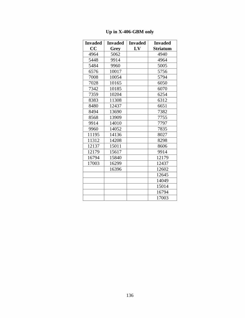
136

Up in X-406-GBM only

Invaded

CC

Invaded

Grey

Invaded

LV

Invaded

Striatum

4964 5062 4940

5448 9914 4964

5484 9960 5005

6576 10017 5756

7008 10054 5794

7028 10165 6050

7342 10185 6070

7359 10204 6254

8383 11308 6312

8480 12437 6651

8494 13690 7382

8568 13909 7755

9914 14010 7797

9960 14052 7835

11195 14136 8027

11312 14208 8298

12137 15011 8606

12179 15617 9914

16794 15840 12179

17003 16299 12437

16396 12602

12645

14049

15014

16794

17003

137

Down in X-406-GBM only

Invaded CC Invaded Grey Invaded LV Invaded Striatum

3042 3752 3238 3215

4458 3826 3438 4052

4771 3877 3934 4304

5320 3898 4474 4329

5600 5317 4767 4338

5900 5756 5045 4388

6444 6312 5268 4419

6704 7654 6444 4769

7246 7683 6951 5046

7506 7754 7069 5062

8647 7797 10185 5269

8776 8026 10203 5317

8840 8107 15012 6369

9081 8143 15849 6443

9781 8198 7198

10095 8237 7506

10844 8297 8774

12772 8339 10055

8494 10163

8774 10185

8985 10203

9081 10299

9244 10375

10469 10469

10630 12772

12601

17203

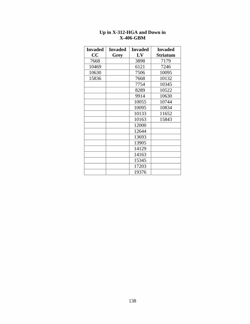
138

Up in X-312-HGA and Down in

X-406-GBM

Invaded

CC

Invaded

Grey

Invaded

LV

Invaded

Striatum

7668

3898 7179

10469

6121 7246

10630

7506 10095

15836

7668 10132

7754 10345

8289 10522

9914 10630

10055 10744

10095 10834

10133 11652

10163 15843

12000

12644

13693

13905

14129

14163

15345

17203

19376

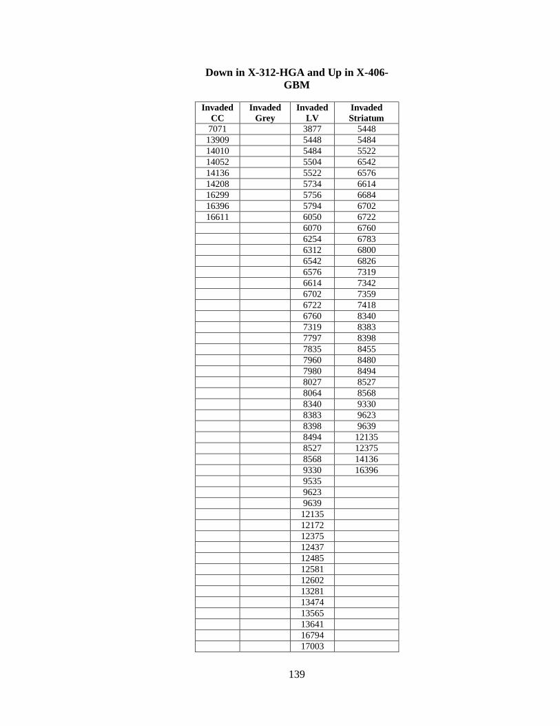
139

Down in X-312-HGA and Up in X-406-

GBM

Invaded

CC

Invaded

Grey

Invaded

LV

Invaded

Striatum

7071

3877 5448

13909

5448 5484

14010

5484 5522

14052

5504 6542

14136

5522 6576

14208

5734 6614

16299

5756 6684

16396

5794 6702

16611

6050 6722

6070 6760

6254 6783

6312 6800

6542 6826

6576 7319

6614 7342

6702 7359

6722 7418

6760 8340

7319 8383

7797 8398

7835 8455

7960 8480

7980 8494

8027 8527

8064 8568

8340 9330

8383 9623

8398 9639

8494 12135

8527 12375

8568 14136

9330 16396

9535

9623

9639

12135

12172

12375

12437

12485

12581

12602

13281

13474

13565

13641

16794

17003

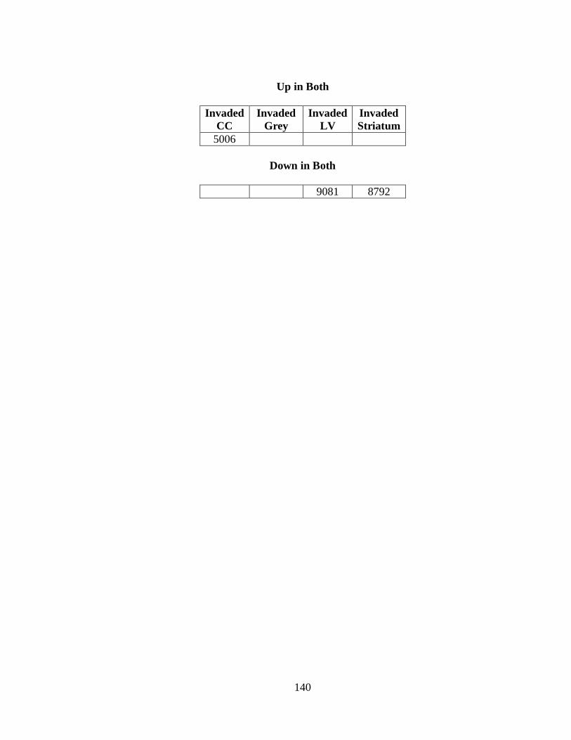
140

Up in Both

Invaded

CC

Invaded

Grey

Invaded

LV

Invaded

Striatum

5006

Down in Both

9081 8792

141

LITERATURE CITED

1. Kennedy, T., Managing the drug discovery/development interface. Drug

Discovery Today 1997, 2 (10), 436-444.

2. Drug Discovery Handbook. John Wiley & Sons, Inc.: 2005.

3. Fee, R., The Cost of Clinical Trials. Drug Discovery and Development 2007.

4. Novartis www.novartis.com/research/drug-discovery.shtml. (accessed 9/17/2010).

5. Canavan, N., Warning!...Warning! Drug Discovery and Development 2007.

6. FDA Investigational New Drug (IND) Application. (accessed 9-17-2010).

7. Health, U. S. N. I. o. ClinicalTrials.gov. (accessed 9/17/2010).

8. FDA New Drug Application. (accessed 9-17-2010).

9. Rieke, G. H., Detection of Light: From the Ultraviolet to the Submillimeter. 2nd

edition ed.; NY Cambridge University Press: New York, 2003.

http://www.netlibrary.com.proxy.library.vanderbilt.edu/Reader/.

10. Gwynne, P.; Heebner, G., Mass Spectrometry in Drug Discovery and

Development: From Physics to Pharma. Science 2006.

11. Cox, K. A.; White, R. E.; Korfmacher, W. A., Rapid determination of

pharmacokinetic properties of new chemical entities: In vivo approaches. Combinatorial

Chemistry & High Throughput Screening 2002, 5 (1), 29-37.

12. Poon, G. K.; Kwei, G.; Wang, R.; Lyons, K.; Chen, Q.; Didolkar, V.; Hop, C.,

Integrating qualitative and quantitative liquid chromatography/tandem mass

spectrometric analysis to support drug discovery. Rapid Communications in Mass

Spectrometry 1999, 13 (19), 1943-1950.

13. Ma, S. G.; Chowdhury, S. K.; Alton, K. B., Application of mass spectrometry for

metabolite identification. Current Drug Metabolism 2006, 7 (5), 503-523.

14. Chen, Y.; Monshouwer, M.; Fitch, W. L., Analytical tools and approaches for

metabolite identification in early drug discovery. Pharmaceutical Research 2007, 24 (2),

248-257.

15. Briggs, D.; Hearn, M. J., Sub-micron molecular imaging-A viability study by

Time-of-Flight SIMS. Surface and Interface Analysis 1988, 13 (4), 181-&.

142

16. Levisetti, R., Recent Applications of High-Resolution Secondary-Ion-Mass-

Spectrometry Imaging Microanalysis Vacuum 1990, 41 (7-9), 1598-1600.

17. Matsuo, J.; Ninomiya, S.; Yamada, H.; Ichiki, K.; Wakamatsu, Y.; Hada, M.;

Seki, T.; Aoki, T., SIMS with highly excited primary beams for molecular depth profiling

and imaging of organic and biological materials. Surface and Interface Analysis 42 (10-

11), 1612-1615.

18. Dass, C., Principles and Practice of Biological Mass Spectrometry. 2001.

19. Schwartz, S. A.; Reyzer, M. L.; Caprioli, R. M., Direct tissue analysis using

matrix-assisted laser desorption/ionization mass spectrometry: practical aspects of sample

preparation. Journal of Mass Spectrometry 2003, 38 (7), 699-708.

20. Chaurand, P.; Schwartz, S. A.; Caprioli, R. M., Profiling and imaging proteins in

tissue sections by MS. Analytical Chemistry 2004, 76 (5), 86A-93A.

21. Chaurand, P.; Schwartz, S. A.; Billheimer, D.; Xu, B. G. J.; Crecelius, A.;

Caprioli, R. M., Integrating histology and imaging mass spectrometry. Analytical

Chemistry 2004, 76 (4), 1145-1155.

22. Aerni, H. R.; Cornett, D. S.; Caprioli, R. M., Automated acoustic matrix

deposition for MALDI sample preparation. Analytical Chemistry 2006, 78 (3), 827-834.

23. Groseclose, M. R.; Andersson, M.; Hardesty, W. M.; Caprioli, R. M.,

Identification of proteins directly from tissue: in situ tryptic digestions coupled with

imaging mass spectrometry. Journal of Mass Spectrometry 2007, 42 (2), 254-262.

24. Baluya, D. L.; Garrett, T. J.; Yost, R. A., Automated MALDI matrix deposition

method with inkjet printing for imaging mass spectrometry. Analytical Chemistry 2007,

79 (17), 6862-6867.

25. Guo, J. In Discovery of Biomarkers for Endometria Carcinoma by Direct

Profiling of Proteins in Tissue Sections, ASMS, San Antonio, TX, San Antonio, TX,

2005.

26. Schuerenberg, M.; Luebbert, C.; Deininger, S.-O.; Ketterlinus, R.; Detlev;

Suckau, D., MALDI tissue imaging: mass spectrometric localization of biomarkers in

tissue slices. Nature Methods 2007, 4 (5), iii.

27. Nye, G. J.; Norris, J. L.; Nickerson, S. In Optimization of the Performance of

Automated Matrix Spraying for MALDI Imaging Mass Spectrometry, ASMS, Seattle,

WA, Seattle, WA, 2006.

28. Mamyrin, B. A., Laser assisted reflectron time-of-flight mass spectrometry.

International Journal of Mass Spectrometry and Ion Processes 1994, 131, 1-19.

143

29. Khatib-Shahidi, S.; Andersson, M.; Herman, J. L.; Gillespie, T. A.; Caprioli, R.

M., Direct molecular analysis of whole-body animal tissue sections by imaging MALDI

mass spectrometry. Analytical Chemistry 2006, 78 (18), 6448-6456.

30. Li, Y.; Shrestha, B.; Vertes, A., Atmospheric pressure molecular imaging by

infrared MALDI mass spectrometry. Analytical Chemistry 2007, 79 (2), 523-532.

31. McLean, J. A.; Ridenour, W. B.; Caprioli, R. M., Profiling and imaging of tissues

by imaging ion mobility-mass spectrometry. Journal of Mass Spectrometry 2007, 42 (8),

1099-1105.

32. Taban, I. M.; Altelaar, A. F. M.; Van der Burgt, Y. E. M.; McDonnell, L. A.;

Heeren, R. M. A.; Fuchser, J.; Baykut, G., Imaging of peptides in the rat brain using

MALDI-FTICR mass spectrometry. Journal of the American Society for Mass

Spectrometry 2007, 18 (1), 145-151.

33. Altelaar, A. F. M.; Taban, I. M.; McDonnell, L. A.; Verhaert, P.; de Lange, R. P.

J.; Adan, R. A. H.; Mooi, W. J.; Heeren, R. M. A.; Piersma, S. R., High-resolution

MALDI imaging mass spectrometry allows localization of peptide distributions at

cellular length scales in pituitary tissue sections. International Journal of Mass

Spectrometry 2007, 260 (2-3), 203-211.

34. Verhaert, P. D.; Conaway, M. C. P.; Pekar, T. M.; Miller, K., Neuropeptide

imaging on an LTQ with vMALDI source: The complete 'all-in-one' peptidome analysis.

International Journal of Mass Spectrometry 2007, 260 (2-3), 177-184.

35. DeKeyser, S. S.; Kutz-Naber, K. K.; Schmidt, J. J.; Barrett-Wilt, G. A.; Li, L. J.,

Imaging mass spectrometry of neuropeptides in decapod crustacean neuronal tissues.

Journal of Proteome Research 2007, 6 (5), 1782-1791.

36. Hanahan, D.; Weinberg, R. A., The hallmarks of cancer. Cell 2000, 100 (1), 57-

70.

37. Stoeckli, M.; Chaurand, P.; Hallahan, D. E.; Caprioli, R. M., Imaging mass

spectrometry: A new technology for the analysis of protein expression in mammalian

tissues. Nature Medicine 2001, 7 (4), 493-496.

38. Reyzer, M. L.; Caldwell, R. L.; Dugger, T. C.; Forbes, J. T.; Ritter, C. A.; Guix,

M.; Arteaga, C. L.; Caprioli, R. M., Early changes in protein expression detected by mass

spectrometry predict tumor response to molecular therapeutics. Cancer Research 2004,

64 (24), 9093-9100.

39. Chaurand, P.; Sanders, M. E.; Jensen, R. A.; Caprioli, R. M., Proteomics in

diagnostic pathology - Profiling and imaging proteins directly in tissue sections.

American Journal of Pathology 2004, 165 (4), 1057-1068.

144

40. Johnson, M. D.; Floyd, J. L.; Caprioli, R. M., Proteomics in Diagnostic

Neuropathology. Journal of Neuropathology and Experimental Neurology 2006, 65 (9),

837-845.

41. Schwamborn, K.; Krieg, R. C.; Reska, M.; Jakse, G.; Knuechel, R.; Wellmann,

A., Identifying prostate carcinoma by MALDI-Imaging. International Journal of

Molecular Medicine 2007, 20, 155-159.

42. Walgren, J. L.; Thompson, D. C., Application of proteomic technologies in the

drug development process. Toxicology Letters 2004, 149 (1-3), 377-385.

43. Lewin, D. A.; Weiner, M. P., Molecular biomarkers in drug development. Drug

Discovery Today 2004, 9 (22), 976-983.

44. Rudin, M.; Rausch, M.; Stoeckli, M., Molecular imaging in drug discovery and

development: Potential and limitations of nonnuclear methods. Molecular Imaging and

Biology 2005, 7 (1), 5-13.

45. Hsieh, Y.; Chen, J.; Korfmacher, W. A., Mapping pharmaceuticals in tissues

using MALDI imaging mass spectrometry. Journal of Pharmacological and

Toxicological Methods 2007, 55 (2), 193-200.

46. Meistermann, H.; Norris, J. L.; Aerni, H.-R.; Cornett, D. S.; Friedlein, A.;

Erskine, A. R.; Augustin, A.; De Vera Mudry, M. C.; Ruepp, S.; Suter, L.; Langen, H.;

Caprioli, R. M.; Ducret, A., Biomarker discovery by imaging mass spectrometry:

Transthyretin is a biomarker for gentamicin-induced nephrotoxicity in rat. Mol Cell

Proteomics 2006, M500399-MCP200.

47. Chandana, S.; Movva, S.; Arora, M.; Singh, T., Primary Brain Tumors in Adults.

American Family Physician 2008, 77 (10), 1423-1430.

48. Laerum, O. D.; Bjerkvig, R.; Steinsvag, S. K.; Ridder, L. d., Invasiveness of

primary brain tumors. Cancer Metastasis Reviews 1984, 3, 223-236.

49. Cunliffe, C. H.; Fischer, I.; Parag, Y.; Fowkes, M. E., State-of-the-Art Pathology:

New WHO Classification, Implications, and New Developments. Neuroimaging Clinics

of North America 20 (3), 259-271.

50. Janny, P.; Cure, H.; Mohr, M.; Heldt, N.; Kwiatkowski, F.; Lemaire, J. J.; Plagne,

R.; Rozan, R., Low grade supratentorial astrocytomas. Management and prognostic

factors. Wiley Subscription Services, Inc., A Wiley Company: 1994; Vol. 73, pp 1937-

1945.

51. Piepmeier, J.; Christopher, S.; Spencer, D.; Byrne, T.; Kim, J.; Knisel, J. P.; Lacy,

J.; Tsukerman, L.; Makuch, R., Variations in the Natural History and Survival of Patients

with Supratentorial Low-grade Astrocytomas. Neurosurgery 1996, 38 (5), 872-879.

145

52. Frueh, F. W., A New Approach for Clinical Trials. Drug discovery and

Development 2010.

53. Atkinson Jr, A. J.; Colburn, W. A.; DeGruttola, V. G.; DeMets, D. L.; Downing,

G. J.; Hoth, D. F.; Oates, J. A.; Peck, C. C.; Schooley, R. T.; Spilker, B. A.; Woodcock,

J.; Zeger, S. L., Biomarkers and surrogate endpoints: preferred definitions and conceptual

framework. Clincial Pharmacology & Therapeutics 2001, 69, 89-95.

54. Zhang, H.; Chan, D. W., Cancer biomarker discovery in plasma using a tissue-

targeted proteomic approach. Cancer Epidemiol Biomarkers Prev 2007, 16 (10), 1915-7.

55. Simpson, R. J.; Bernhard, O. K.; Greening, D. W.; Moritz, R. L., Proteomics-

driven cancer biomarker discovery: looking to the future. Curr Opin Chem Biol 2008, 12

(1), 72-7.

56. Etzioni, R.; Urban, N.; Ramsey, S.; McIntosh, M.; Schwartz, S.; Reid, B.; Radich,

J.; Anderson, G.; Hartwell, L., The case for early detection. Nat Rev Cancer 2003, 3 (4),

243-52.

57. Nolen, B. M.; Marks, J. R.; Ta'san, S.; Rand, A.; Luong, T. M.; Wang, Y.;

Blackwell, K.; Lokshin, A. E., Serum biomarker profiles and response to neoadjuvant

chemotherapy for locally advanced breast cancer. Breast Cancer Res 2008, 10 (3), R45.

58. Schuerenberg, M.; Luebbert, C.; Deininger, S. O.; Ketterlinus, R.; Suckau, D.,

MALDI tissue imaging: mass spectrometric localization of biomarkers in tissue slices.

Nature Methods 2007, 4 (5), iii-iv.

59. Zhang, H.; Wu, G.; Tu, H.; Huang, F., Discovery of serum biomarkers in

astrocytoma by SELDI–TOF MS and proteinchip technology. Journal of Neuro-

Oncology 2007, 84 (3), 315-323.

60. Ilyin, S. E.; Belkowski, S. M.; Plata-Salamán, C. R., Biomarker discovery and

validation: technologies and integrative approaches. Trends in Biotechnology 2004, 22

(8), 411-416.

61. MALDI MS: A Practical Guide to Instrumentation, Methods and Applications.

Weily-VCH: Munster Germany, 2007.

62. ProteomeDigest The Internal Standard.

http://www.ionsource.com/tutorial/msquan/is.htm (accessed 10/6/2010).

63. MacDougall, D.; Crummett, W. B., Guidelines for data acquisition and data

quality evaluation in environmental chemistry. Analytical Chemistry 1980, 52 (14), 2242-

2249.

146

64. Armbruster, D.; Tillman, M.; Hubbs, L., Limit of detection (LQD)/limit of

quantitation (LOQ): comparison of the empirical and the statistical methods exemplified

with GC-MS assays of abused drugs. Clin Chem 1994, 40 (7), 1233-1238.

65. Aravagiri, M.; Teper, Y.; Marder, S. R., Pharmacokinetics and tissue distribution

of olanzapine in rats. John Wiley & Sons, Ltd.: 1999; Vol. 20, pp 369-377.

66. Bogusz, M. J.; Krüger, K. D.; Maier, R. D.; Erkwoh, R.; Tuchtenhagen, F.,

Monitoring of olanzapine in serum by liquid chromatography-atmospheric pressure

chemical ionization mass spectrometry. Journal of Chromatography B: Biomedical

Sciences and Applications 1999, 732 (2), 257-269.

67. Bao, J.; Potts, B. D., Quantitative determination of olanzapine in rat brain tissue

by high-performance liquid chromatography with electrochemical detection. Journal of

Chromatography B: Biomedical Sciences and Applications 2001, 752 (1), 61-67.

68. Central Brain Tumor Registry of the United States. Statistical report: primary

brain tumors in the United States, 2000-2004. http://www.cbtrus.org/reports//2007-

2008/2007report.pdf (accessed September 26, 2010).

69. Wen, P. Y.; Kesari, S., Malignant Gliomas in Adults. New England Journal of

Medicine 2008, 359 (5), 492-507.

70. Croom, K. F.; Perry, C. M., Imatinib Mesylate: In the Treatment of

Gastrointestinal Stromal Tumours. Drugs 2003, 63 (5), 513-522.

71. Druker, B. J., Perspectives on the development of a molecularly targeted agent.

Cancer Cell 2002, 1 (1), 31-36.

72. DiRocco, F.; Carroll, R. S.; Zhang, J.; Black, P., Platelet-derived Growth Factor

and Its Receptor Expression in Human Oligodendrogliomas. Neurosurgery 1998, 42 (2),

341-346.

73. Deuel, T. F.; Huang, J. S., Platelet-derived growth factor. Structure, function, and

roles in normal and transformed cells. The Journal of Clinical Investigation 1984, 74 (3),

669-676.

74. Hermanson, M.; Funa, K.; Hartman, M.; Claesson-Welsh, L.; Heldin, C.-H.;

Westermark, B.; Nister, M., Platelet-derived Growth Factor and Its Receptors in Human

Glioma Tissue: Expression of Messenger RNA and Protein Suggests the Presence of

Autocrine and Paracrine Loops. Cancer Research 1992, 52 (11), 3213-3219.

75. Lokker, N. A.; Sullivan, C. M.; Hollenbach, S. J.; Israel, M. A.; Giese, N. A.,

Platelet-derived Growth Factor (PDGF) Autocrine Signaling Regulates Survival and

Mitogenic Pathways in Glioblastoma Cells. Cancer Research 2002, 62 (13), 3729-3735.

147

76. Kilic, T.; Alberta, J. A.; Zdunek, P. R.; Acar, M.; Iannarelli, P.; O’Reilly, T.;

Buchdunger, E.; Black, P. M.; Stiles, C. D., Intracranial Inhibition of Platelet-derived

Growth Factor-mediated Glioblastoma Cell Growth by an Orally Active Kinase Inhibitor

of the 2-Phenylaminopyrimidine Class. Cancer Research 2000, 60 (18), 5143-5150.

77. Hagerstrand, D.; Hesselager, G.; Achterberg, S.; Wickenberg Bolin, U.;

Kowanetz, M.; Kastemar, M.; Heldin, C. H.; Isaksson, A.; Nister, M.; Ostman, A.,

Characterization of an imatinib-sensitive subset of high-grade human glioma cultures.

Oncogene 2006, 25 (35), 4913-4922.

78. Cao, R.; Rakenhielm, E.; Li, X.; Pietras, K.; Widenfalk, J.; Ostman, A.; Eriksson,

U.; Cao, Y., Angiogenesis stimulated by PDGF-CC, a novel member in the PDGF

family, involves activation of PDGFR-{alpha}{alpha} and -{alpha}{beta} receptors.

FASEB J. 2002, 16 (12), 1575-1583.

79. Geng, L.; Shinohara, E. T.; Kim, D.; Tan, J.; Osusky, K.; Shyr, Y.; Hallahan, D.

E., STI571 (Gleevec) improves tumor growth delay and survival in irradiated mouse

models of glioblastoma. Int J Radiat Oncol Biol Phys 2006, 64 (1), 263-71.

80. United States Department of Agriculture, Transportation, Sale and Handling of

Certain Animals. . AAPHI, Ed. 2010.

81. Online Ethics Center for Engineering and Research, The Ethics of Using Animals

in Research. http://www.onlineethics.org/CMS/2963/modindex/animalres.aspx (accessed

September 26, 2010).

82. OLAW Applied Research Ethics National Association, Institutional Animal Care

and Use Committee Guidebook. Pitts, M., Ed. 1992.

http://grants.nih.gov/grants/olaw/GuideBook.pdf.

83. Handbook of Laboratory Animal Science, Second Edition. CRC Press LLC: 2003;

Vol. II.

84. Candolfi, M.; Curtin, J.; King, G. D.; Pluhar, E.; McNiel, E.; Ohlfest, J. R.;

Freese, A. B.; Moore, P. F.; Nichols, S. W.; Lowenstein, P. R.; Castro, M. G.,

Glioblastoma multiforme (GBM): a comparative histological analysis of gliomas in mice,

rats, dogs and humans. AACR Meeting Abstracts 2006, 2006 (1), 642.

85. Kamphorst, W.; deBoer, A. G.; Gaillard, P. J., Brain Drug Targeting: The Future

of Brain Drug Development. University Press: Cambridge, 2001.

86. Denysenko, T.; Gennero, L.; Roos, M. A.; Melcarne, A.; Juenemann, C.; Faccani,

G.; Morra, I.; Cavallo, G.; Reguzzi, S.; Pescarmona, G.; Ponzetto, A., Glioblastoma

cancer stem cells: heterogeneity, microenvironment and related therapeutic strategies.

John Wiley & Sons, Ltd.: Vol. 28, pp 343-351.

148

87. Inda, M. D.; Bonavia, R.; Mukasa, A.; Narita, Y.; Sah, D. W. Y.; Vandenberg, S.;

Brennan, C.; Johns, T. G.; Bachoo, R.; Hadwiger, P.; Tan, P.; DePinho, R. A.; Cavenee,

W.; Furnari, F., Tumor heterogeneity is an active process maintained by a mutant EGFR-

induced cytokine circuit in glioblastoma. Genes Dev. 24 (16), 1731-1745.

88. Park, D. M.; Rich, J. N., Biology of glioma cancer stem cells. Mol. Cells 2009, 28

(1), 7-12.

89. Teoh, M.; Narayanan, P.; Moo, K.; Radhakrisman, S.; Pillappan, R.; Bukhari, N.;

Segarra, I., HPLC Determination Of Imatinib In Plasma And Tissues After

Multiple Oral DoseAdministration To Mice. Pakistan Journal of Pharmaceutical

Sciences 2010, 23 (1), 35-41.

90. Parise, R. A.; Ramanathan, R. K.; Hayes, M. J.; Egorin, M. J., Liquid

chromatographic-mass spectrometric assay for quantitation of imatinib and its main

metabolite (CGP 74588) in plasma. Journal of Chromatography B 2003, 791 (1-2), 39-

44.

91. Tusher, V. G.; Tibshirani, R.; Chu, G., Significance analysis of microarrays

applied to the ionizing radiation response. Proceedings of the National Academy of

Sciences 2001, 98 (9), 5116-5121.

92. Asotra, K.; Ningaraj, N.; Black, K., The Blood-Brain Barrier: Measurement of

Blood-Brain and Blood-Tumor Barrier Permeabilities with [14C]-Labeled Tracers.

Methods in Molecular Medicine 2003, 89 (11), 177-190.

93. Lockman, P. R.; Mittapalli, R. K.; Taskar, K. S.; Rudraraju, V.; Gril, B.; Bohn, K.

A.; Adkins, C. E.; Roberts, A.; Thorsheim, H. R.; Gaasch, J. A.; Huang, S.; Palmieri, D.;

Steeg, P. S.; Smith, Q. R., Heterogeneous Blood–Tumor Barrier Permeability

Determines Drug Efficacy in Experimental Brain Metastases of Breast Cancer. Clinical

Cancer Research 16 (23), 5664-5678.

94. Stewart, D. J., A critique of the role of the blood-brain barrier in the

chemotherapy of human brain tumors. Journal of Neuro-Oncology 1994, 20 (2), 121-139.

95. Holdhoff, M.; Supko, J.; Gallia, G.; Hann, C.; Bonekamp, D.; Ye, X.; Cao, B.;

Olivi, A.; Grossman, S., Intratumoral concentrations of imatinib after oral administration

in patients with glioblastoma multiforme. Journal of Neuro-Oncology 97 (2), 241-245.

96. Gschwind, H.-P.; Pfaar, U.; Waldmeier, F.; Zollinger, M.; Sayer, C.; Zbinden, P.;

Hayes, M.; Pokorny, R.; Seiberling, M.; Ben-Am, M.; Peng, B.; Gross, G.,

METABOLISM AND DISPOSITION OF IMATINIB MESYLATE IN HEALTHY

VOLUNTEERS. Drug Metabolism and Disposition 2005, 33 (10), 1503-1512.

97. Van Erp, N. P.; Gelderblom, H.; Guchelaar, H.-J., Clinical pharmacokinetics of

tyrosine kinase inhibitors. Cancer Treatment Reviews 2009, 35 (8), 692-706.

149

98. Kramer, T., Side Effects and Therapeutic Effects: Half-life and Steady State.

Medscape General Medicine 2003, 5 (1).

99. Landriscina, M.; Maddalena, F.; Laudiero, G.; Esposito, F., Adaptation to

Oxidative Stress, Chemoresistance, and Cell Survival. Antioxid. Redox Signal. 2009, 11

(11), 2701-2716.

100. Voet, D.; Voet, J. G., Biochemistry, Second Edition. John Wiley & Sons, Inc:

New York, 1995.

101. Chakravarti, A.; Chakladar, A.; Delaney, M. A.; Latham, D. E.; Loeffler, J. S.,

The Epidermal Growth Factor Receptor Pathway Mediates Resistance to Sequential

Administration of Radiation and Chemotherapy in Primary Human Glioblastoma Cells in

a RAS-dependent Manner. Cancer Research 2002, 62 (15), 4307-4315.

102. Servidei, T.; Riccardi, A.; Sanguinetti, M.; Dominici, C.; Riccardi, R., Increased

sensitivity to the platelet-derived growth factor (PDGF) receptor inhibitor STI571 in

chemoresistant glioma cells is associated with enhanced PDGF-BB-mediated signaling

and STI571-induced Akt inactivation. Wiley Subscription Services, Inc., A Wiley

Company: 2006; Vol. 208, pp 220-228.

103. Ziegler, D. S.; Wright, R. D.; Kesari, S.; Lemieux, M. E.; Tran, M. A.; Jain, M.;

Zawel, L.; Kung, A. L., Resistance of human glioblastoma multiforme cells to growth

factor inhibitors is overcome by blockade of inhibitor of apoptosis proteins. The Journal

of Clinical Investigation 2008, 118 (9), 3109-3122.

104. Oliva, C. R.; Nozell, S. E.; Diers, A.; McClugage, S. G.; Sarkaria, J. N.; Markert,

J. M.; Darley-Usmar, V. M.; Bailey, S. M.; Gillespie, G. Y.; Landar, A.; Griguer, C. E.,

Acquisition of Temozolomide Chemoresistance in Gliomas Leads to Remodeling of

Mitochondrial Electron Transport Chain. J. Biol. Chem. 285 (51), 39759-39767.

105. Kennedy, F. G.; Jones, D. P., Oxygen Dependence of Mitochondrial-Function in

Isolated Rat Cardiac Myocytes. American Journal of Physiology 1986, 250 (3), C374-

C383.

106. Villani, G.; Greco, M.; Papa, S.; Attardi, G., Low Reserve of Cytochrome c

Oxidase Capacity in Vivo in the Respiratory Chain of a Variety of Human Cell Types. J.

Biol. Chem. 1998, 273 (48), 31829-31836.

107. Brozzi, F.; Arcuri, C.; Giambanco, I.; Donato, R., S100B Protein Regulates

Astrocyte Shape and Migration via Interaction with Src Kinase: Implications for

Astrocyte Development, Activation and Tumor Growth J. Biol. Chem. 2009, 284 (13),

8788-8802.

108. Vos, M. J.; Postma, T. J.; Martens, F.; Uitdehaag, B. M. J.; Blankenstein, M. A.;

Vandertop, W. P.; Slotman, B. J.; Heimans, J. J., Serum Levels of S-100B Protein and

150

Neuron-specific Enolase in Glioma Patients: A Pilot Study. Anticancer Research 2004,

24 (4), 2511-2514.

109. Selinfreund, R. H.; Barger, S. W.; Welsh, M. J.; Van Eldik, L. J., Antisense

inhibition of glial S100 beta production results in alterations in cell morphology,

cytoskeletal organization, and cell proliferation. The Journal of Cell Biology 1990, 111

(5), 2021-2028.

110. George, J. M., The synucleins. Genome Biology 2001, 3 (1).

111. Liu, H.; Liu, W.; Wu, Y.; Zhou, Y.; Xue, R.; Luo, C.; Wang, L.; Zhao, W.; Jiang,

J.-D.; Liu, J., Loss of Epigenetic Control of Synuclein-γ Gene as a Molecular Indicator

of Metastasis in a Wide Range of Human Cancers. Cancer Research 2005, 65 (17), 7635-

7643.

112. Crews, L.; Tsigelny, I.; Hashimoto, M.; Masliah, E., Role of Synucleins in

Alzheimer's Disease. Neurotox. Res. 2009, 16 (3), 306-317.

113. Fung, K.-M.; Rorke, L. B.; Giasson, B.; Lee, V. M. Y.; Trojanowski, J. Q.,

Expression of a-, ß-, and gamma-synuclein in glial tumors and medulloblastomas. Acta

Neuropathologica 2003, 106 (2), 167-175.

114. Surguchov, A., Focus on Molecules: The synucleins: "When friends become

foes". Experimental Eye Research 2008, 86 (1), 1-2.

115. Maniatis, T.; Reed, R., The role of small nuclear ribonucleoprotein particles in

pre-mRNA splicing. Nature 1987, 325 (6106), 673-678.

116. Cheung, H.; Baggerly, K.; Tsavachidis, S.; Bachinski, L.; Neubauer, V.; Nixon,

T.; Aldape, K.; Cote, G.; Krahe, R., Global analysis of aberrant pre-mRNA splicing in

glioblastoma using exon expression arrays. BMC Genomics 2008, 9 (1), 216.

117. Kasai, T.; Inoue, M.; Koshiba, S.; Yabuki, T.; Aoki, M.; Nunokawa, E.; Seki, E.;

Matsuda, T.; Matsuda, N.; Tomo, Y.; Shirouzu, M.; Terada, T.; Obayashi, N.; Hamana,

H.; Shinya, N.; Tatsuguchi, A.; Yasuda, S.; Yoshida, M.; Hirota, H.; Matsuo, Y.; Tani,

K.; Suzuki, H.; Arakawa, T.; Carninci, P.; Kawai, J.; Hayashizaki, Y.; Kigawa, T.;

Yokoyama, S., Solution structure of a BolA-like protein from Mus musculus. Cold

Spring Harbor Laboratory Press: 2004; Vol. 13, pp 545-548.

118. Burton, M.; Rose, T. M.; Faergeman, N. J.; Knudsen, J., Evolution of the acyl-

CoA binding protein (ACBP). Biochem. J. 2005, 392, 299-307.

119. Coté, R. J., Aseptic Technique for Cell Culture. John Wiley & Sons, Inc.: 2001.

120. Norris, J. L.; Cornett, D. S.; Mobley, J. A.; Andersson, M.; Seeley, E. H.;

Chaurand, P.; Caprioli, R. M., Processing MALDI mass spectra to improve mass spectral

151

direct tissue analysis. International Journal of Mass Spectrometry 2007, 260 (2-3), 212-

221.

121. Clement, V.; Sanchez, P.; de Tribolet, N.; Radovanovic, I.; Ruiz i Altaba, A.,

HEDGEHOG-GLI1 Signaling Regulates Human Glioma Growth, Cancer Stem Cell Self-

Renewal, and Tumorigenicity. Current biology : CB 2007, 17 (2), 165-172.

122. Ruiz i Altaba, A.; Sanchez, P.; Dahmane, N., Gli and hedgehog in cancer:

tumours, embryos and stem cells. Nat Rev Cancer 2002, 2 (5), 361-372.

123. Jessell, T. M., Neuronal specification in the spinal cord: inductive signals and

transcriptional codes. Nat Rev Genet 2000, 1 (1), 20-29.

124. Ruiz i Altaba, A.; Palma, V.; Dahmane, N., Hedgehog-GLI signaling and the

growth of the brain. Nat Rev Neurosci 2002, 3 (1), 24-33.

125. Ruiz i Altaba, A.; Stecca, B.; Sánchez, P., Hedgehog-Gli signaling in brain

tumors: stem cells and paradevelopmental programs in cancer. Cancer Letters 2004, 204

(2), 145-157.

126. Xu, Q.; Yuan, X.; Liu, G.; Black, K. L.; Yu, J. S., Hedgehog Signaling Regulates

Brain Tumor-Initiating Cell Proliferation and Portends Shorter Survival for Patients with

PTEN-Coexpressing Glioblastomas. John Wiley & Sons, Ltd.: 2008; Vol. 26, pp 3018-

3026.

127. Becher, O. J.; Hambardzumyan, D.; Fomchenko, E. I.; Momota, H.; Mainwaring,

L.; Bleau, A.-M.; Katz, A. M.; Edgar, M.; Kenney, A. M.; Cordon-Cardo, C.; Blasberg,

R. G.; Holland, E. C., Gli Activity Correlates with Tumor Grade in Platelet-Derived

Growth Factor-Induced Gliomas. Cancer Res 2008, 68 (7), 2241-2249.

128. Wang, k.; Pan, L.; Che, X.; Cui, D.; Li, C., Sonic Hedgehog/GLI1 signaling

pathway inhibition restricts cell migration and invasion in human gliomas. Neurological

Research 2010, 32 (9), 975-980.

129. Wang, K.; Pan, L.; Che, X.; Cui, D.; Li, C., Gli1 inhibition induces cell-cycle

arrest and enhanced apoptosis in brain glioma cell lines. Journal of Neuro-Oncology

2010, 98 (3), 319-327.

130. Sarangi, A.; Valadez, J. G.; Rush, S.; Abel, T. W.; Thompson, R. C.; Cooper, M.

K., Targeted inhibition of the Hedgehog pathway in established malignant glioma

xenografts enhances survival. Oncogene 2009, 28 (39), 3468-3476.

131. Bar, E. E.; Chaudhry, A.; Lin, A.; Fan, X.; Schreck, K.; Matsui, W.; Piccirillo, S.;

Vescovi, A. L.; DiMeco, F.; Olivi, A.; Eberhart, C. G., Cyclopamine-Mediated Hedgehog

Pathway Inhibition Depletes Stem-Like Cancer Cells in Glioblastoma. John Wiley &

Sons, Ltd.: 2007; Vol. 25, pp 2524-2533.

152

132. UCDavis Mouse in Science Cancer Research.

http://www.vetmed.ucdavis.edu/Animal_alternatives/cancer.htm (accessed September 26,

2010).

133. Candolfi, M.; Curtin, J.; Nichols, W.; Muhammad, A. K. M.; King, G.; Pluhar,

G.; McNiel, E.; Ohlfest, J.; Freese, A.; Moore, P.; Lerner, J.; Lowenstein, P.; Castro, M.,

Intracranial glioblastoma models in preclinical neuro-oncology: neuropathological

characterization and tumor progression. Journal of Neuro-Oncology 2007, 85 (2), 133-

148.

134. Zheng, X.; Cui, X.-X.; Avila, G. E.; Huang, M.-T.; Liu, Y.; Patel, J.; Kong, A. N.

T.; Paulino, R.; Shih, W. J.; Lin, Y.; Rabson, A. B.; Reddy, B. S.; Conney, A. H.,

Atorvastatin and Celecoxib Inhibit Prostate PC-3 Tumors in Immunodeficient Mice.

Clinical Cancer Research 2007, 13 (18), 5480-5487.

135. Heikkila, J. E.; Vaha-Koskela, M. J. V.; Ruotsalainen, J. J.; Martikainen, M. W.;

Stanford, M. M.; McCart, J. A.; Bell, J. C.; Hinkkanen, A. E., Intravenously

Administered Alphavirus Vector VA7 Eradicates Orthotopic Human Glioma Xenografts

in Nude Mice. PLoS ONE 5 (1), e8603.

136. Niclou, S. P.; Danzeisen, C.; Eikesdal, H. P.; Wiig, H.; Brons, N. H. C.; Poli, A.

M. F.; Svendsen, A.; Torsvik, A.; Enger, P. O.; Terzis, J. A.; Bjerkvig, R., A novel eGFP-

expressing immunodeficient mouse model to study tumor-host interactions. FASEB J.

2008, 22 (9), 3120-3128.

137. O/'Brien, C. A.; Pollett, A.; Gallinger, S.; Dick, J. E., A human colon cancer cell

capable of initiating tumour growth in immunodeficient mice. Nature 2007, 445 (7123),

106-110.

138. Charafe-Jauffret, E.; Ginestier, C.; Birnbaum, D., Breast cancer stem cells: tools

and models to rely on. BMC Cancer 2009, 9 (1), 202.

139. Yang, Z. F.; Ho, D. W.; Ng, M. N.; Lau, C. K.; Yu, W. C.; Ngai, P.; Chu, P. W.

K.; Lam, C. T.; Poon, R. T. P.; Fan, S. T., Significance of CD90+ Cancer Stem Cells in

Human Liver Cancer. Cancer Cell 2008, 13 (2), 153-166.

140. Dong, X.; Guan, J.; English, J. C.; Flint, J.; Yee, J.; Evans, K.; Murray, N.;

MacAulay, C.; Ng, R. T.; Gout, P. W.; Lam, W. L.; Laskin, J.; Ling, V.; Lam, S.; Wang,

Y., Patient-Derived First Generation Xenografts of Non–Small Cell Lung Cancers:

Promising Tools for Predicting Drug Responses for Personalized Chemotherapy. Clinical

Cancer Research 16 (5), 1442-1451.

141. Lee, J.; Kotliarova, S.; Kotliarov, Y.; Li, A.; Su, Q.; Donin, N. M.; Pastorino, S.;

Purow, B. W.; Christopher, N.; Zhang, W.; Park, J. K.; Fine, H. A., Tumor stem cells

derived from glioblastomas cultured in bFGF and EGF more closely mirror the

153

phenotype and genotype of primary tumors than do serum-cultured cell lines. Cancer

Cell 2006, 9 (5), 391-403.

142. Lipinski, R. J.; Hutson, P. R.; Hannam, P. W.; Nydza, R. J.; Washington, I. M.;

Moore, R. W.; Girdaukas, G. G.; Peterson, R. E.; Bushman, W., Dose- and route-

dependent teratogenicity, toxicity, and pharmacokinetic profiles of the Hedgehog

signaling antagonist cyclopamine in the mouse. Toxicological Sciences 2008, 104 (1),

189-197.

143. Lewis, P. M.; Gritli-Linde, A.; Smeyne, R.; Kottmann, A.; McMahon, A. P.,

Sonic hedgehog signaling is required for expansion of granule neuron precursors and

patterning of the mouse cerebellum. Developmental Biology 2004, 270 (2), 393-410.

144. Fingar, D. C.; Blenis, J., Target of rapamycin (TOR): an integrator of nutrient and

growth factor signals and coordinator of cell growth and cell cycle progression.

Oncogene 23 (18), 3151-3171.

145. Sancak, Y.; Bar-Peled, L.; Zoncu, R.; Markhard, A. L.; Nada, S.; Sabatini, D. M.,

Ragulator-Rag Complex Targets mTORC1 to the Lysosomal Surface and Is Necessary

for Its Activation by Amino Acids. Cell 141 (2), 290-303.

146. Sanchez, P.; Ruiz i Altaba, A., In vivo inhibition of endogenous brain tumors

through systemic interference of Hedgehog signaling in mice. Mechanisms of

Development 2005, 122 (2), 223-230.

147. Rehman, I.; Azzouzi, A. R.; Cross, S. S.; Deloulme, J. C.; Catto, J. W. F.; Wylde,

N.; Larre, S.; Champigneuille, J.; Hamdy, F. C., Dysregulated expression of S100A11

(Calgizzarin) in prostate cancer and precursor lesions. Hum. Pathol. 2004, 35 (11), 1385-

1391.

148. Melle, C.; Ernst, G.; Schimmel, B.; Bleul, A.; Mothes, H.; Kaufmann, R.;

Settmacher, U.; von Eggeling, F., Different expression of calgizzarin (S100A11) in

normal colonic epithelium, adenoma and colorectal carcinoma. Int. J. Oncol. 2006, 28

(1), 195-200.

149. Ohuchida, K.; Mizumoto, K.; Ohhashi, S.; Yamaguchi, H.; Konomi, H.; Nagai,

E.; Yamaguchi, K.; Tsuneyoshi, M.; Tanaka, M., S100A11, a putative tumor suppressor

gene, is overexpressed in pancreatic carcinogenesis. Clinical Cancer Research 2006, 12

(18), 5417-5422.

150. Liu, X. G.; Wang, X. P.; Li, W. F.; Yang, S.; Zhou, X.; Li, S. J.; Li, X. J.; Hao, D.

Y.; Fan, Z. M., Ca2+-binding protein S100A11: A novel diagnostic marker for breast

carcinoma. Oncol. Rep. 23 (5), 1301-1308.

151. Kanamori, T.; Takakura, K.; Mandai, M.; Kariya, M.; Fukuhara, K.; Sakaguchi,

M.; Huh, N.-h.; Saito, K.; Sakurai, T.; Fujita, J.; Fujii, S., Increased expression of

154

calcium-binding protein S100 in human uterine smooth muscle tumours. Molecular

Human Reproduction 2004, 10 (10), 735-742.

152. Cecconi, D.; Donadelli, M.; Rinalducci, S.; Zolla, L.; Scupoli, M. T.; Scarpa, A.;

Palmieri, M.; Righetti, P. G., Proteomic analysis of pancreatic endocrine tumor cell lines

treated with the histone deacetylase inhibitor trichostatin A. Wiley-vch Verlag: 2007;

Vol. 7, pp 1644-1653.

153. Turrens, J. F., Mitochondrial formation of reactive oxygen species. The Journal of

Physiology 2003, 552 (2), 335-344.

154. Wang, Y.; Fang, J.; Leonard, S. S.; Krishna Rao, K. M., Cadmium inhibits the

electron transfer chain and induces Reactive Oxygen Species. Free Radical Biology and

Medicine 2004, 36 (11), 1434-1443.

155. McClintock, D. S.; Santore, M. T.; Lee, V. Y.; Brunelle, J.; Budinger, G. R. S.;

Zong, W.-X.; Thompson, C. B.; Hay, N.; Chandel, N. S., Bcl-2 Family Members and

Functional Electron Transport Chain Regulate Oxygen Deprivation-Induced Cell Death.

Mol. Cell. Biol. 2002, 22 (1), 94-104.

156. Chen, Y.; McMillan-Ward, E.; Kong, J.; Israels, S. J.; Gibson, S. B.,

Mitochondrial electron-transport-chain inhibitors of complexes I and II induce

autophagic cell death mediated by reactive oxygen species. J Cell Sci 2007, 120 (23),

4155-4166.

157. Azad, M. B.; Chen, Y.; Gibson, S. B., Regulation of autophagy by reactive

oxygen species (ROS): implications for cancer progression and treatment. Antioxidants

&amp; Redox Signaling 2009, 11 (4), 777(14).

158. Ruy, F.; Vercesi, A.; Kowaltowski, A., Inhibition of specific electron transport

pathways leads to oxidative stress and decreased proliferation. Journal of Bioenergetics

and Biomembranes 2006, 38 (2), 129-135.

159. Chen, Y. Q.; Gibson, S. B., Is mitochondrial generation of reactive oxygen

species a trigger for autophagy? Autophagy 2008, 4 (2), 246-248.

160. Chen, Y.; Azad, M. B.; Gibson, S. B., Superoxide is the major reactive oxygen

species regulating autophagy. Cell Death Differ. 2009, 16 (7), 1040-1052.

161. Welch, K. D.; Panter, K. E.; Lee, S. T.; Gardner, D. R.; Stegelmeier, B. L.; Cook,

D., Cyclopamine-induced synophthalmia in sheep: defining a critical window and

toxicokinetic evaluation. John Wiley & Sons, Ltd.: 2009; Vol. 29, pp 414-421.

162. Li, H.-Y.; Xu, W.; Li, H.-L.; Zhang, W.-D.; Hu, L.-W., LC-MS-MS Method for

the Determination of Protoveratrine A in Rat Plasma. Chromatographia 2009, 69 (5),

523-529.

155

163. Tremblay, M. R.; Lescarbeau, A.; Grogan, M. J.; Tan, E.; Lin, G.; Austad, B. C.;

Yu, L.-C.; Behnke, M. L.; Nair, S. J.; Hagel, M.; White, K.; Conley, J.; Manna, J. D.;

Alvarez-Diez, T. M.; Hoyt, J.; Woodward, C. N.; Sydor, J. R.; Pink, M.; MacDougall, J.;

Campbell, M. J.; Cushing, J.; Ferguson, J.; Curtis, M. S.; McGovern, K.; Read, M. A.;

Palombella, V. J.; Adams, J.; Castro, A. C., Discovery of a Potent and Orally Active

Hedgehog Pathway Antagonist (IPI-926). Journal of Medicinal Chemistry 2009, 52 (14),

4400-4418.

164. Rossi, D. T.; Sinz, M. W., Mass Spectrometry in Drug Discovery. Marcel Dekker,

Inc.: New York, 2002.

165. Contag, P. R., The Development of Biomarkers to Bridge Preclinical and Clinical

Studies. Parma DD 2006, 1 (2).