Embed Size (px)
Citation preview
SEPTEMBER 2001 2721F I N N I G A N E T A L .
q 2001 American Meteorological Society
Response Characteristics of a Buoyancy-Driven Sea
T. D. FINNIGAN, K. B. WINTERS,* AND G. N. IVEY
Centre for Water Research, University of Western Australia, Crawley, Western Australia, Australia
(Manuscript received 3 March 2000, in final form 23 January 2001)
ABSTRACT
The authors consider the flow in a semienclosed sea, or basin, subjected to a destabilizing surface buoyancyflux and separated from a large adjoining reservoir by a sill. A series of numerical experiments were conductedto quantify the energetics of the flow within the basin, that is, the amount of kinetic and potential energy storedwithin the basin and the rate at which these quantities are transported to and from the reservoir via the exchangeflow over the sill. The numerical experiments were formulated at laboratory scales and conducted using aboundary-fitting, clustered grid to resolve the entrainment and mixing processes within the flow and to facilitatequantitative comparison with previous laboratory experiments.
Volume and boundary integrated energetics were computed for both steady and time-varying flows. In thesteady-state limit, the rate of energy flux through the surface is balanced by dissipation within the basin andadvection of potential energy over the sill and into the reservoir. The analyses focus primarily on this latterquantity because it is closely related to the outflow density and volume transport in two-layered exchange flows.Scaling laws relating the energetics of the flow to the surface buoyancy flux and the geometrical scales of thebasin–sill system are derived and validated using the numerical results.
A second set of experiments was conducted to quantify the transient energetics in response to a sudden changein the surface forcing. These results, combined with a linear impulse–response analysis, were used to derive ageneral expression describing the advection of potential energy across the sill for periodically forced systems.The analytical predictions are shown to compare favorably with directly simulated flows and to be reasonablyconsistent with limited field observations of the seasonal variability through the Strait of Bab al Mandab.
1. Introduction
In many semienclosed seas or basins the large-scalecirculation is driven by lateral density gradients. Suchbuoyancy-driven flows exist, for example, where pro-cesses within the sea maintain a net density differencebetween the sea and adjoining ocean, and therefore pro-duce an exchange of fluid between the two. The dy-namics of such systems are of wide interest becausethey influence both local and remote oceanic environ-ments (e.g., Reid 1979). This paper investigates the in-fluence on the large-scale flow of mixing processes with-in a basin (or sea) that is partially separated from a largereservoir (or ocean) by a topographical constriction. Wefocus in particular on an idealized, convectively drivenbasin, that is, one subjected to a loss of surface buoyancydue to cooling, evaporation in excess of fresh inflow,or to the growth of sea ice (Fig. 1). The flow config-uration is generic, and thus has relevance to semien-
*Current affiliation: Applied Physics Laboratory, University ofWashington, Seattle, Washington.
Corresponding author address: T. D. Finnigan, Department of Ocean-ography, MSB 434, University of Hawaii at Manoa, 1000 Pope Road,Honolulu, HI 96822.
closed seas (e.g., the Red Sea), cooling ponds, lake side-arms, and arctic fjords.
There have been several previous studies aimed atmodeling similar systems theoretically (e.g., Stommeland Farmer 1953; Phillips 1966; Maxworthy 1997), inthe laboratory (Harashima and Watanabe 1986; Sturmanand Ivey 1998; Finnigan and Ivey 1999, 2000; Grimmand Maxworthy 1999), and numerically (Kowalik andMatthews 1983). With the exception of Kowalik andMathews (1983), Sturman and Ivey (1998), and Fin-nigan and Ivey (1999), these studies have consideredonly steady flows. Field experiments have also beenconducted, most notably in the Red Sea (Murray andJohns 1997; Smeed 1997) and the Mediterranean Sea(Bray et al. 1995; Bryden and Kinder 1991), showingsome aspects of the spatial structure and temporal var-iability of these unsteadily forced systems, particularlyin the vicinity of the marginal constriction. In the presentwork, we consider both steady and unsteady forcing andcharacterize the spatial and temporal variability of theresulting flow.
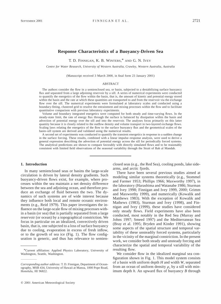
We consider flow in the idealized marginal sea con-figuration shown in Fig. 1. This model system consistsof a basin with uniform depth H and width W, separatedfrom an ocean of uniform density ro by a sill with min-imum depth h. An upward flux of buoyancy B through
2722 VOLUME 31J O U R N A L O F P H Y S I C A L O C E A N O G R A P H Y
FIG. 1. A buoyancy-driven marginal sea. A sill at x 5 L restrictsthe exchange flow between the sea and the adjoining ocean.
the surface of the basin (0 # x # L, 0 # y # W, z 5H) results in a lateral density gradient across the silland a consequent buoyancy-driven response.
The surface forcing can be thought of as a flux ofavailable potential energy into the basin. Some of thisenergy is converted to kinetic energy, associated withboth turbulent motions and large-scale circulation andwith the exchange flow over the sill. As we will show,an energetics analysis leads to a general description ofboth the steady and unsteady flow behavior. The poten-tial and kinetic energy stored within the basin, and theflux of these quantities across the sill, can be simplyrelated to the external parameters (B, L, W, H, h). Wefocus in particular on the flux of potential energy fromthe basin, over the sill, and into the adjoining reservoirbecause this is the energetics quantity most closely re-lated to volumetric and scalar transport. This approachcan be applied generally; it does not require that theexchange be reasonably approximated by a layeredstructure, and thus can be used to quantify the exchangein continuously sheared and stratified flows.
We present results from several numerical experi-ments based on solutions to the unsteady governingequations in three dimensions. The numerical methodsand validation experiments are described in section 2.Numerical simulations allow a volumetric and time-de-pendent analysis of the energy storage and conversionrates within the basin, as well as the rates of kinetic andpotential energy flux across the sill. The results are usedto test and validate scaling relationships between energyfluxes and the external parameters characterizing theflow configuration. Steady energetics are described insection 3. The transient response to sudden changes inthe surface forcing is discussed in section 4. An im-pulse–response analysis is used to extend these resultsto an oscillatory (seasonal or diurnal) forcing in section5. Concluding remarks appear in section 6.
2. Numerical experiments
a. Description
In the laboratory experiments of Finnigan and Ivey(2000) it was found that the internal turbulent stress, orReynolds stress, contributes significantly to the basin-scale horizontal momentum balance, which, in turn, de-termines the magnitude of the circulation and therefore
the exchange across the sill. Small-scale processes thusinfluence the large-scale circulation. For the presentstudy we have endeavored to design and implement aseries of numerical experiments that represent, as closeas possible, the relevant range of flow scales present inthese laboratory experiments. To achieve this, the nu-merical experiments were performed on the same spatialscales as laboratory experiments and high-order meth-ods were employed to solve the unsteady governingequations with fine spatial and temporal resolution (seebelow). Direct comparisons between laboratory and nu-merical results provide confidence in the numerical sim-ulations, which are then used to expand the parameterrange of the experiments and verify scaling laws basedon external parameters. This ultimately leads to a set ofgeneral scaling laws that may be used to model the flowresponse in actual full-scale systems.
Numerical experiments offer a number of conve-niences. First, by specifying a semibounded domain weavoid the finite volume restrictions inherent to labora-tory experiments. Simulation of slowly varying un-steady flows is thus possible. Furthermore, numericalexperiments provide full three-dimensional data fieldsfrom which to compute volume and boundary integratedenergetics. Finally, the forcing and geometrical param-eters can be varied to investigate their effects.
b. Methods
The simulations are based on the equations of motionfor incompressible density-stratified flow,
]u 1 gr91 u · =u 5 2 =p 2 z 1 = · K =u, (1)m]t r r0 0
]r91 u · =r9 5 = · K =r9, (2)r]t
= · u 5 0, (3)
where u 5 (u, y, w) is the velocity vector in Cartesian(x, y, z) coordinates, r9 is the density perturbation abouta constant value ro, p is the perturbation about hydro-static pressure in a fluid with density r(x, y, z, t) 5 ro
1 r9(x, y, z, t), g is the gravitational acceleration, andz is the unit vector in the vertical direction z (positiveupward). The coefficients Km and Kr are the diffusioncoefficients for momentum and density, respectively.
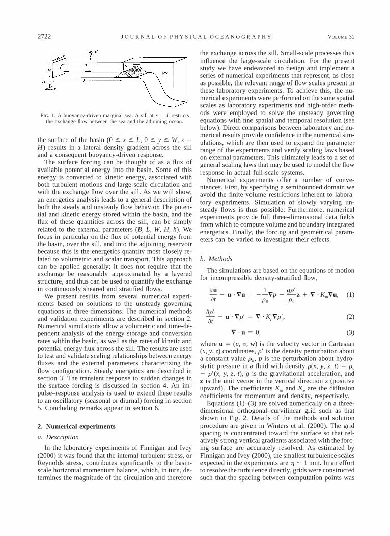
Equations (1)–(3) are solved numerically on a three-dimensional orthogonal–curvilinear grid such as thatshown in Fig. 2. Details of the methods and solutionprocedure are given in Winters et al. (2000). The gridspacing is concentrated toward the surface so that rel-atively strong vertical gradients associated with the forc-ing surface are accurately resolved. As estimated byFinnigan and Ivey (2000), the smallest turbulence scalesexpected in the experiments are h ; 1 mm. In an effortto resolve the turbulence directly, grids were constructedsuch that the spacing between computation points was
SEPTEMBER 2001 2723F I N N I G A N E T A L .
FIG. 2. Example of a numerical grid used in the simulations. This grid had 129 3 17 3 33computational nodes. For longer basins, grids with 257 3 17 3 33 nodes were used.
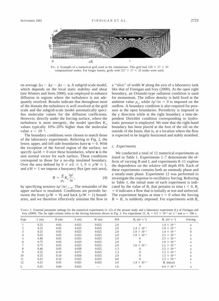
TABLE 1. External parameter settings for the numerical experiments (1–12) of the present study and a laboratory experiment (L) of Finnigan andIvey (2000). The far right column refers to the forcing functions shown in Fig. 3. For experiment 12, Bs 5 0.5 3 1026 m2 s23 and v 5 390 s.
Expt L (m) H (m) h (m) W (m) H/h Bo (m2 s23) B` (m2 s23) Forcing
123456789
101112
0.250.250.250.250.460.750.750.460.250.250.250.25
0.050.050.050.050.050.050.050.050.100.100.100.05
0.0250.0250.0250.0250.0250.0250.0250.0380.0750.0500.0250.025
0.0250.0250.0250.0250.0250.0250.0250.0250.0250.0250.0250.025
2.02.02.02.02.02.02.01.31.32.04.02.0
01.4 3 1026
1.9 3 1026
1.9 3 1026
00
1.6 3 1026
0000
1.4 3 1026
1.4 3 1026
1.9 3 1026
1.4 3 1026
2.5 3 1026
2.5 3 1026
1.6 3 1026
2.1 3 1026
2.5 3 1026
1.5 3 1026
1.5 3 1026
1.5 3 1026
Bs sin(vt)
aabaaaaaaaac
L 0.25 0.04 0.025 — 1.6 0 0.4 3 1026 a
on average Dx ; Dy ; Dz ; h. A subgrid-scale model,which depends on the local static stability and shear(see Winters and Seim 2000), was employed to enhancediffusion in regions where the turbulence is not ade-quately resolved. Results indicate that throughout mostof the domain the turbulence is well resolved at the gridscale and the subgrid-scale model automatically speci-fies molecular values for the diffusion coefficients.However, directly under the forcing surface, where theturbulence is most energetic, the model specifies Km
values typically 10%–20% higher than the molecularvalue n 5 1026.
The boundary conditions were chosen to match thoseof the laboratory experiments. Referring to Fig. 2, thelower, upper, and left side boundaries have u 5 0. Withthe exception of the forced region of the surface, wespecify ]r/]n 5 0 over these boundaries, where n is theunit normal vector for each surface. These conditionscorrespond to those for a no-slip insulated boundary.Over the area defined by 0 # x/L # 1, 0 # y/W # 1,and z/H 5 1 we impose a buoyancy flux (per unit area),
g ]r9B 5 K , (4)rr ]z0
by specifying nonzero ]r9/]z | z5H. The remainder of theupper surface is insulated. Conditions are periodic be-tween the front (y/W 5 0) and back (y/W 5 1) bound-aries, and we therefore effectively simulate the flow in
a ‘‘slice’’ of width W along the axis of a laboratory tanklike that of Finnigan and Ivey (2000). At the open rightboundary, an Orlanski-type radiation condition is usedfor momentum. The inflow density is held fixed at theambient value ro, while ]r9/]x 5 0 is imposed on theoutflow. A boundary condition is also required for pres-sure at the open boundaries. Periodicity is imposed inthe y direction while at the right boundary a time-de-pendent Dirichlet condition corresponding to hydro-static pressure is employed. We note that the right-handboundary has been placed at the foot of the sill on theoutside of the basin, that is, at a location where the flowis expected to be largely horizontal and stably stratified.
c. Experiments
We conducted a total of 12 numerical experiments aslisted in Table 1. Experiments 1–7 demonstrate the ef-fects of varying B and L and experiments 8–11 explorethe dependence on the relative sill depth H/h. Each ofthese experiments contains both an unsteady phase anda steady-state phase. Experiment 12 was performed toinvestigate the response to oscillatory forcing. Referringto Table 1, the initial state of each experiment is indi-cated by the value of Bo that pertains to time t , 0. Bo
5 0 indicates a flow that is initially at rest and unforced.The experiment begins at time t 5 0 when the forcingB 5 B` is suddenly imposed. For experiments with Bo
2724 VOLUME 31J O U R N A L O F P H Y S I C A L O C E A N O G R A P H Y
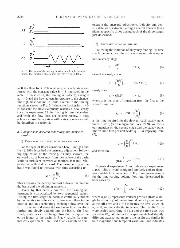
FIG. 3. The form of the forcing functions used in the presentstudy. The functions shown here are referred to in Table 1.
± 0 the flow for t , 0 is already at steady state andforced with the constant value B 5 Bo indicated in thetable. In these cases, the forcing is suddenly changedat t 5 0 and the flow adjusts in response to the change.The rightmost column in Table 1 refers to the forcingfunctions shown in Fig. 3. Where the forcing for t . 0is constant the flow eventually reaches a new steadystate. In experiment 12 the forcing is time dependentand while the flow does not become steady, it doesachieve an oscillatory state with a steady mean as willbe described in section 5.
d. Comparisons between laboratory and numericalresults
1) TEMPORAL AND SPATIAL FLOW FEATURES
For the type of flows considered here, Finnigan andIvey (1999) described the unsteady adjustment follow-ing application of the forcing. As they showed, theoutward flux of buoyancy from the surface of the basinleads to turbulent convective motions that mix rela-tively dense fluid downward. The mean density of thebasin was found to increase with time according to
r Btor ; . (5)g H
This increases the density contrast between the fluid inthe basin and the adjoining reservoir.
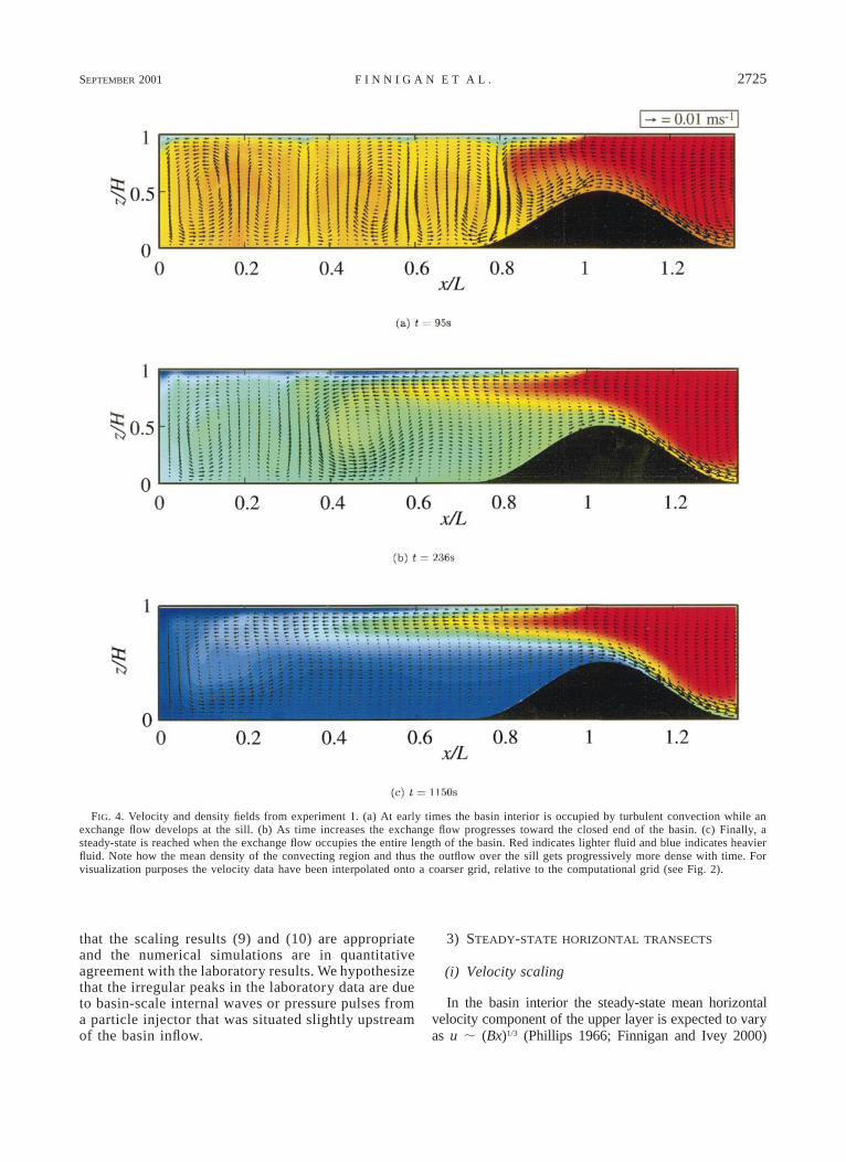
Driven by this density contrast, the ensuing ad-justment is characterized by two sequential stages.During the first stage the basin is continually mixedby convective turbulence with zero mean flow in theinterior and an accelerating exchange flow over thesill. In the second stage the exchange flow developsfurther and slowly extends into the basin. The finalsteady state has an exchange flow that occupies theentire length of the basin. In Fig. 4 results from nu-merical experiment 1 are used as an example to dem-
onstrate the unsteady adjustment. Velocity and den-sity data were extracted along a central vertical (x–z)plane at specific times during each of the three stagesjust described.
2) UNSTEADY FLOW AT THE SILL
Following the initiation of buoyancy forcing B at timet 5 0 the velocity at the sill was shown to develop as
first unsteady stage:
2Btu ; , t & t (6)tl
second unsteady stage:
1/2Bhtu ; , t & t & t (7)t ss1 2H
steady state:1/3u ; (BL) , t * t (8)ss
where tt is the time of transition from the first to thesecond stage and
H2/3 21/3t ; L B (9)ss 1 2h
is the time required for the flow to reach steady state.Since tt K ttt (see Finnigan and Ivey 1999), we focusour attention on the second stage and the steady state.The volume flux per unit width q ; uh implying from(7),
1/2Bt3/2q ; h , (10)1 2H
and therefore,
q1/2; t . (11)
1/2 3/2(B /H ) h
Numerical experiment 1 and laboratory experimentL (see Table 1) were configured similarly and are there-fore suitable for comparison. In Fig. 5 we present resultsfor the time-varying volume flow rate, determined inboth cases by
H
q(t) 5 u (z, t) dz, (12)E s
i
where us (z, t) represents vertical profiles (from a sin-gle location in y) of the horizontal velocity componentat the sill crest and z 5 i indicates the level at whichus 5 0, or the velocity interface. The results for qwere scaled according to (11) and the time axis wasscaled as t/t ss . While the two experiments had slightlydifferent external parameters the results are similar inboth magnitude and temporal variation. This indicates
SEPTEMBER 2001 2725F I N N I G A N E T A L .
FIG. 4. Velocity and density fields from experiment 1. (a) At early times the basin interior is occupied by turbulent convection while anexchange flow develops at the sill. (b) As time increases the exchange flow progresses toward the closed end of the basin. (c) Finally, asteady-state is reached when the exchange flow occupies the entire length of the basin. Red indicates lighter fluid and blue indicates heavierfluid. Note how the mean density of the convecting region and thus the outflow over the sill gets progressively more dense with time. Forvisualization purposes the velocity data have been interpolated onto a coarser grid, relative to the computational grid (see Fig. 2).
that the scaling results (9) and (10) are appropriateand the numerical simulations are in quantitativeagreement with the laboratory results. We hypothesizethat the irregular peaks in the laboratory data are dueto basin-scale internal waves or pressure pulses froma particle injector that was situated slightly upstreamof the basin inflow.
3) STEADY-STATE HORIZONTAL TRANSECTS
(i) Velocity scaling
In the basin interior the steady-state mean horizontalvelocity component of the upper layer is expected to varyas u ; (Bx)1/3 (Phillips 1966; Finnigan and Ivey 2000)
2726 VOLUME 31J O U R N A L O F P H Y S I C A L O C E A N O G R A P H Y
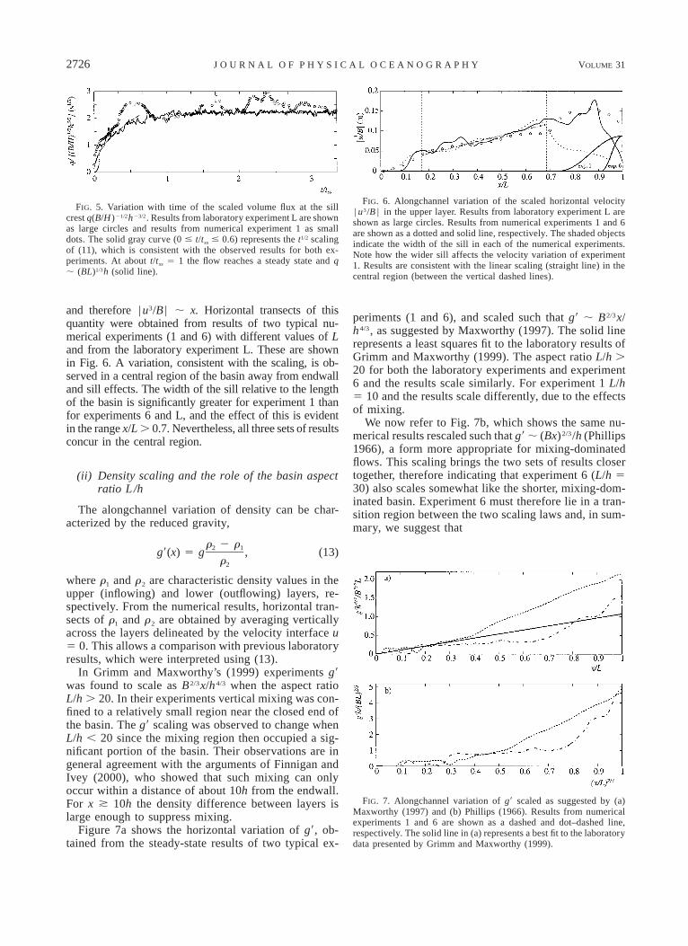
FIG. 5. Variation with time of the scaled volume flux at the sillcrest q(B/H )21/2h23/2. Results from laboratory experiment L are shownas large circles and results from numerical experiment 1 as smalldots. The solid gray curve (0 # t/tss # 0.6) represents the t1/2 scalingof (11), which is consistent with the observed results for both ex-periments. At about t/tss 5 1 the flow reaches a steady state and q; (BL)1/3h (solid line).
FIG. 6. Alongchannel variation of the scaled horizontal velocity| u3/B | in the upper layer. Results from laboratory experiment L areshown as large circles. Results from numerical experiments 1 and 6are shown as a dotted and solid line, respectively. The shaded objectsindicate the width of the sill in each of the numerical experiments.Note how the wider sill affects the velocity variation of experiment1. Results are consistent with the linear scaling (straight line) in thecentral region (between the vertical dashed lines).
FIG. 7. Alongchannel variation of g9 scaled as suggested by (a)Maxworthy (1997) and (b) Phillips (1966). Results from numericalexperiments 1 and 6 are shown as a dashed and dot–dashed line,respectively. The solid line in (a) represents a best fit to the laboratorydata presented by Grimm and Maxworthy (1999).
and therefore | u3/B | ; x. Horizontal transects of thisquantity were obtained from results of two typical nu-merical experiments (1 and 6) with different values of Land from the laboratory experiment L. These are shownin Fig. 6. A variation, consistent with the scaling, is ob-served in a central region of the basin away from endwalland sill effects. The width of the sill relative to the lengthof the basin is significantly greater for experiment 1 thanfor experiments 6 and L, and the effect of this is evidentin the range x/L . 0.7. Nevertheless, all three sets of resultsconcur in the central region.
(ii) Density scaling and the role of the basin aspectratio L /h
The alongchannel variation of density can be char-acterized by the reduced gravity,
r 2 r2 1g9(x) 5 g , (13)r2
where r1 and r2 are characteristic density values in theupper (inflowing) and lower (outflowing) layers, re-spectively. From the numerical results, horizontal tran-sects of r1 and r2 are obtained by averaging verticallyacross the layers delineated by the velocity interface u5 0. This allows a comparison with previous laboratoryresults, which were interpreted using (13).
In Grimm and Maxworthy’s (1999) experiments g9was found to scale as B2/3x/h4/3 when the aspect ratioL/h . 20. In their experiments vertical mixing was con-fined to a relatively small region near the closed end ofthe basin. The g9 scaling was observed to change whenL/h , 20 since the mixing region then occupied a sig-nificant portion of the basin. Their observations are ingeneral agreement with the arguments of Finnigan andIvey (2000), who showed that such mixing can onlyoccur within a distance of about 10h from the endwall.For x * 10h the density difference between layers islarge enough to suppress mixing.
Figure 7a shows the horizontal variation of g9, ob-tained from the steady-state results of two typical ex-
periments (1 and 6), and scaled such that g9 ; B2/3x/h4/3, as suggested by Maxworthy (1997). The solid linerepresents a least squares fit to the laboratory results ofGrimm and Maxworthy (1999). The aspect ratio L/h .20 for both the laboratory experiments and experiment6 and the results scale similarly. For experiment 1 L/h5 10 and the results scale differently, due to the effectsof mixing.
We now refer to Fig. 7b, which shows the same nu-merical results rescaled such that g9 ; (Bx)2/3/h (Phillips1966), a form more appropriate for mixing-dominatedflows. This scaling brings the two sets of results closertogether, therefore indicating that experiment 6 (L/h 530) also scales somewhat like the shorter, mixing-dom-inated basin. Experiment 6 must therefore lie in a tran-sition region between the two scaling laws and, in sum-mary, we suggest that
SEPTEMBER 2001 2727F I N N I G A N E T A L .
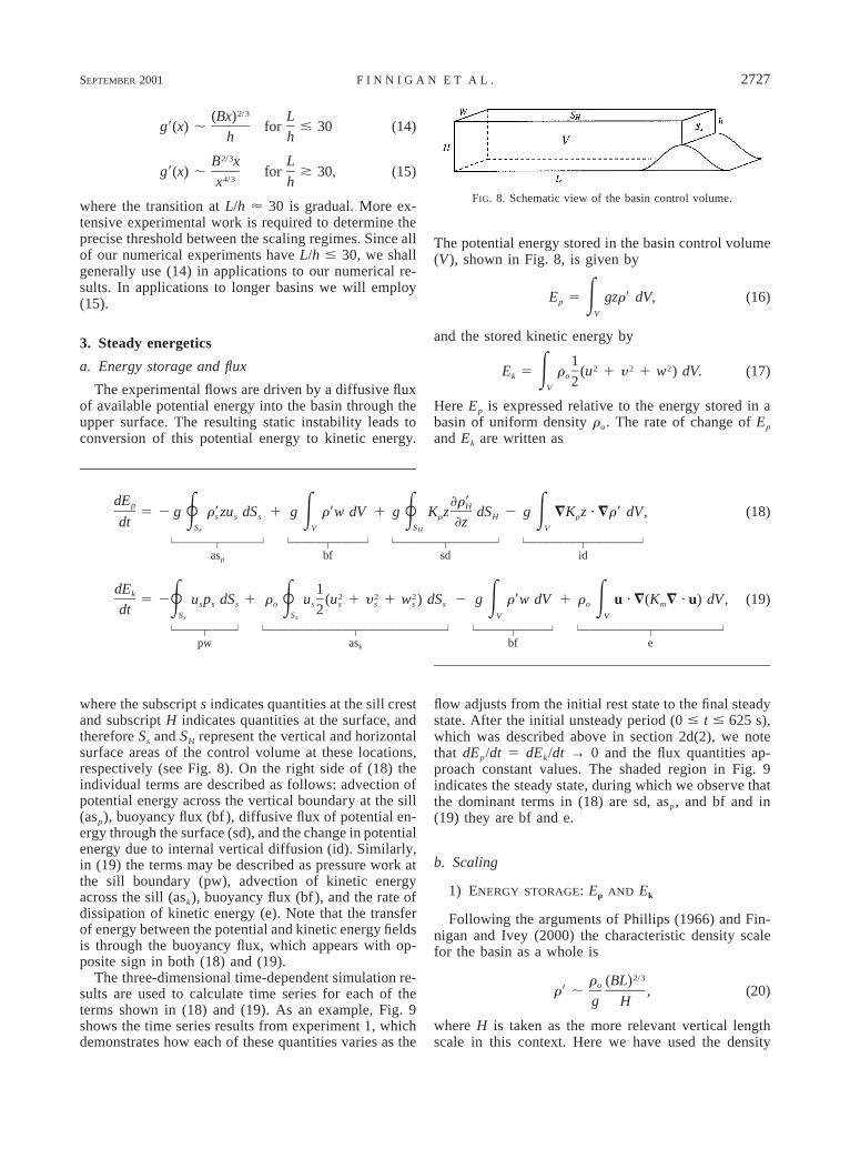
FIG. 8. Schematic view of the basin control volume.
2/3(Bx) Lg9(x) ; for & 30 (14)
h h2/3B x L
g9(x) ; for * 30, (15)4/3x h
where the transition at L/h ø 30 is gradual. More ex-tensive experimental work is required to determine theprecise threshold between the scaling regimes. Since allof our numerical experiments have L/h # 30, we shallgenerally use (14) in applications to our numerical re-sults. In applications to longer basins we will employ(15).
3. Steady energetics
a. Energy storage and flux
The experimental flows are driven by a diffusive fluxof available potential energy into the basin through theupper surface. The resulting static instability leads toconversion of this potential energy to kinetic energy.
The potential energy stored in the basin control volume(V), shown in Fig. 8, is given by
E 5 gzr9 dV, (16)p EV
and the stored kinetic energy by
12 2 2E 5 r (u 1 y 1 w ) dV. (17)k E o 2V
Here Ep is expressed relative to the energy stored in abasin of uniform density ro. The rate of change of Ep
and Ek are written as
dE ]r9p H5 2 g r9zu dS 1 g r9w dV 1 g K z dS 2 g =K z · =r9 dV, (18)R s s s E R r H E rdt ]zS SV Vs H
| | | | | | | |}}}}}}} }}}}}} }}}}}}}} }}}}}}}}}z z z z
as bf sd idp
dE 1k 2 2 25 2 u p dS 1 r u (u 1 y 1 w ) dS 2 g r9w dV 1 r u · =(K = · u) dV , (19)R s s s o R s s s s s E o E mdt 2S S V Vs s
| | | | | | | |}}}}} }}}}}}}}}}}}}} }}}}}} }}}}}}}}}}}z z z z
pw as bf ek
where the subscript s indicates quantities at the sill crestand subscript H indicates quantities at the surface, andtherefore Ss and SH represent the vertical and horizontalsurface areas of the control volume at these locations,respectively (see Fig. 8). On the right side of (18) theindividual terms are described as follows: advection ofpotential energy across the vertical boundary at the sill(asp), buoyancy flux (bf ), diffusive flux of potential en-ergy through the surface (sd), and the change in potentialenergy due to internal vertical diffusion (id). Similarly,in (19) the terms may be described as pressure work atthe sill boundary (pw), advection of kinetic energyacross the sill (ask), buoyancy flux (bf ), and the rate ofdissipation of kinetic energy (e). Note that the transferof energy between the potential and kinetic energy fieldsis through the buoyancy flux, which appears with op-posite sign in both (18) and (19).
The three-dimensional time-dependent simulation re-sults are used to calculate time series for each of theterms shown in (18) and (19). As an example, Fig. 9shows the time series results from experiment 1, whichdemonstrates how each of these quantities varies as the
flow adjusts from the initial rest state to the final steadystate. After the initial unsteady period (0 # t # 625 s),which was described above in section 2d(2), we notethat dEp/dt 5 dEk/dt → 0 and the flux quantities ap-proach constant values. The shaded region in Fig. 9indicates the steady state, during which we observe thatthe dominant terms in (18) are sd, asp, and bf and in(19) they are bf and e.
b. Scaling
1) ENERGY STORAGE: Ep AND Ek
Following the arguments of Phillips (1966) and Fin-nigan and Ivey (2000) the characteristic density scalefor the basin as a whole is
2/3r (BL)or9 ; , (20)g H
where H is taken as the more relevant vertical lengthscale in this context. Here we have used the density
2728 VOLUME 31J O U R N A L O F P H Y S I C A L O C E A N O G R A P H Y
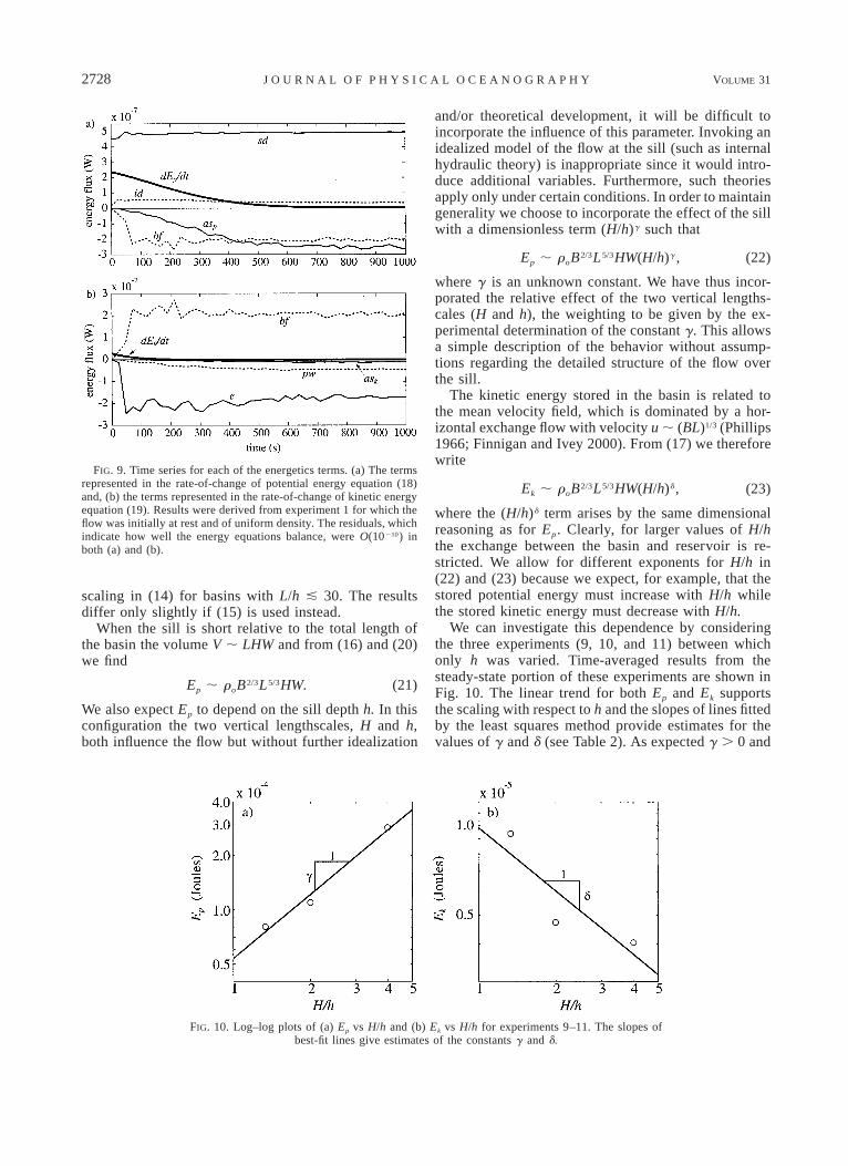
FIG. 9. Time series for each of the energetics terms. (a) The termsrepresented in the rate-of-change of potential energy equation (18)and, (b) the terms represented in the rate-of-change of kinetic energyequation (19). Results were derived from experiment 1 for which theflow was initially at rest and of uniform density. The residuals, whichindicate how well the energy equations balance, were O(10210) inboth (a) and (b).
FIG. 10. Log–log plots of (a) Ep vs H/h and (b) Ek vs H/h for experiments 9–11. The slopes ofbest-fit lines give estimates of the constants g and d.
scaling in (14) for basins with L/h & 30. The resultsdiffer only slightly if (15) is used instead.
When the sill is short relative to the total length ofthe basin the volume V ; LHW and from (16) and (20)we find
2/3 5/3E ; r B L HW.p o (21)
We also expect Ep to depend on the sill depth h. In thisconfiguration the two vertical lengthscales, H and h,both influence the flow but without further idealization
and/or theoretical development, it will be difficult toincorporate the influence of this parameter. Invoking anidealized model of the flow at the sill (such as internalhydraulic theory) is inappropriate since it would intro-duce additional variables. Furthermore, such theoriesapply only under certain conditions. In order to maintaingenerality we choose to incorporate the effect of the sillwith a dimensionless term (H/h)g such that
2/3 5/3 gE ; r B L HW(H/h) ,p o (22)
where g is an unknown constant. We have thus incor-porated the relative effect of the two vertical lengths-cales (H and h), the weighting to be given by the ex-perimental determination of the constant g. This allowsa simple description of the behavior without assump-tions regarding the detailed structure of the flow overthe sill.
The kinetic energy stored in the basin is related tothe mean velocity field, which is dominated by a hor-izontal exchange flow with velocity u ; (BL)1/3 (Phillips1966; Finnigan and Ivey 2000). From (17) we thereforewrite
2/3 5/3 dE ; r B L HW(H/h) ,k o (23)
where the (H/h)d term arises by the same dimensionalreasoning as for Ep. Clearly, for larger values of H/hthe exchange between the basin and reservoir is re-stricted. We allow for different exponents for H/h in(22) and (23) because we expect, for example, that thestored potential energy must increase with H/h whilethe stored kinetic energy must decrease with H/h.
We can investigate this dependence by consideringthe three experiments (9, 10, and 11) between whichonly h was varied. Time-averaged results from thesteady-state portion of these experiments are shown inFig. 10. The linear trend for both Ep and Ek supportsthe scaling with respect to h and the slopes of lines fittedby the least squares method provide estimates for thevalues of g and d (see Table 2). As expected g . 0 and
SEPTEMBER 2001 2729F I N N I G A N E T A L .
TABLE 2. Summary of the main steady-state scaling results. The scaling relations (as numbered in the text) are converted to formulas using theexperimentally determined constants.
Scaling Constants Formulas
(22)(23)(28)(32)
c 5 2.0 6 0.10p
c 5 0.2 6 0.09k
c 5 0.3 6 0.05s
c 5 0.3 6 0.05r
g 5 1.2 6 0.50d 5 20.7 6 0.20l 5 1.0 6 0.10j 5 1.0 6 0.10
2/3 5/3 gE 5 c r B L HW(H/h)p p o
2/3 5/3 dE 5 c r B L HW(H/h)k k o
las 5 c r BLHW(H/h)p s o
21/3 2/3 jt 5 c r DB L (H/h)r r o
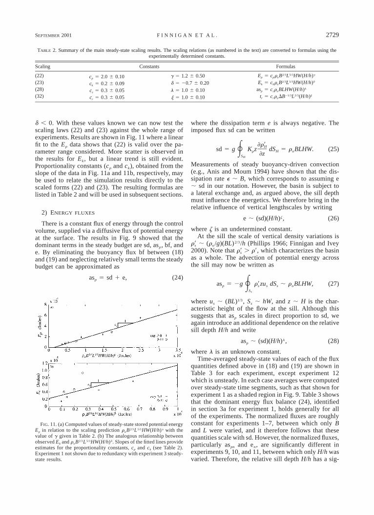
FIG. 11. (a) Computed values of steady-state stored potential energyEp in relation to the scaling prediction roB2/3L5/3HW(H/h)g with thevalue of g given in Table 2. (b) The analogous relationship betweenobserved Ek and roB2/3L5/3HW(H/h)d. Slopes of the fitted lines provideestimates for the proportionality constants, cp and ck (see Table 2).Experiment 1 not shown due to redundancy with experiment 3 steady-state results.
d , 0. With these values known we can now test thescaling laws (22) and (23) against the whole range ofexperiments. Results are shown in Fig. 11 where a linearfit to the Ep data shows that (22) is valid over the pa-rameter range considered. More scatter is observed inthe results for Ek, but a linear trend is still evident.Proportionality constants (cp and ck), obtained from theslope of the data in Fig. 11a and 11b, respectively, maybe used to relate the simulation results directly to thescaled forms (22) and (23). The resulting formulas arelisted in Table 2 and will be used in subsequent sections.
2) ENERGY FLUXES
There is a constant flux of energy through the controlvolume, supplied via a diffusive flux of potential energyat the surface. The results in Fig. 9 showed that thedominant terms in the steady budget are sd, asp, bf, ande. By eliminating the buoyancy flux bf between (18)and (19) and neglecting relatively small terms the steadybudget can be approximated as
as 5 sd 1 e,p (24)
where the dissipation term e is always negative. Theimposed flux sd can be written
]r9Hsd 5 g K z dS 5 r BLHW. (25)R r H o]zSH
Measurements of steady buoyancy-driven convection(e.g., Anis and Moum 1994) have shown that the dis-sipation rate e ; B, which corresponds to assuming e; sd in our notation. However, the basin is subject toa lateral exchange and, as argued above, the sill depthmust influence the energetics. We therefore bring in therelative influence of vertical lengthscales by writing
ze ; (sd)(H/h) , (26)
where z is an undetermined constant.At the sill the scale of vertical density variations is; (ro/g)(BL)2/3/h (Phillips 1966; Finnigan and Iveyr9s
2000). Note that . r9, which characterizes the basinr9sas a whole. The advection of potential energy acrossthe sill may now be written as
as 5 2g r9zu dS ; r BLHW, (27)p R s s s oSs
where us ; (BL)1/3, Ss ; hW, and z ; H is the char-acteristic height of the flow at the sill. Although thissuggests that asp scales in direct proportion to sd, weagain introduce an additional dependence on the relativesill depth H/h and write
las ; (sd)(H/h) ,p (28)
where l is an unknown constant.Time-averaged steady-state values of each of the flux
quantities defined above in (18) and (19) are shown inTable 3 for each experiment, except experiment 12which is unsteady. In each case averages were computedover steady-state time segments, such as that shown forexperiment 1 as a shaded region in Fig. 9. Table 3 showsthat the dominant energy flux balance (24), identifiedin section 3a for experiment 1, holds generally for allof the experiments. The normalized fluxes are roughlyconstant for experiments 1–7, between which only Band L were varied, and it therefore follows that thesequantities scale with sd. However, the normalized fluxes,particularly aspn and en, are significantly different inexperiments 9, 10, and 11, between which only H/h wasvaried. Therefore, the relative sill depth H/h has a sig-
2730 VOLUME 31J O U R N A L O F P H Y S I C A L O C E A N O G R A P H Y
TABLE 3. Energy flux and storage quantities for the numerical exper-iments. Fluxes appear normalized by the forcing flux sd, and storagequantities appear normalized by the total stored energy Ep 1 Ek, for eachindividual experiment.
Expt aspn bfn idn pwn askn en Epn Ekn
123456789
1011
0.520.470.510.580.420.430.340.410.400.620.92
20.4320.4520.4520.6320.4120.6320.9020.4120.8420.7020.71
20.0720.1020.0720.1020.0720.0220.0120.0720.1220.1120.10
0.090.120.120.120.050.070.080.050.190.060.15
0.020.020.020.020.010.030.030.010.060.040.07
20.3420.3320.3720.4120.2520.4020.4020.2520.3220.2120.25
0.980.980.980.970.980.990.980.980.890.960.99
0.020.020.020.030.020.010.020.020.110.040.01
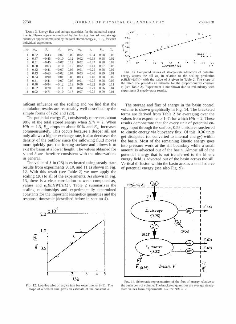
FIG. 13. Computed values of steady-state advection of potentialenergy across the sill asp in relation to the scaling predictionroBLHW(H/h)l with the value of l given in Table 2. The slope ofthe fitted line provides an estimate for the proportionality constantcs (see Table 2). Experiment 1 not shown due to redundancy withexperiment 3 steady-state results.
FIG. 12. Log–log plot of asp vs H/h for experiments 9–11. Theslope of a best-fit line gives an estimate of the constant l.
FIG. 14. Schematic representation of the flux of energy relative tothe basin control volume. The bracketed quantities are average steady-state values from experiments 1–7 for H/h 5 2.
nificant influence on the scaling and we find that thesimulation results are reasonably well described by thesimple forms of (26) and (28).
The potential energy Epn consistently represents about98% of the total stored energy when H/h 5 2. WhenH/h 5 1.3, Epn drops to about 90% and Ekn increasescommensurately. This occurs because a deeper sill notonly allows a higher exchange rate, it also decreases thedensity of the outflow since the inflowing fluid movesmore quickly past the forcing surface and allows it toexit the basin at a lower height. The values obtained forg and d are therefore consistent with the observationsin general.
The value of l in (28) is estimated using steady-stateresults from experiments 9, 10, and 11 as shown in Fig.12. With this result (see Table 2) we now apply thescaling (28) to all of the experiments. As shown in Fig.13, there is a clear correlation between computed asp
values and roBLHW(H/L)l. Table 2 summarizes thescaling relationships and experimentally determinedconstants for the important energetics quantities and theresponse timescale (described below in section 4).
The storage and flux of energy in the basin controlvolume is shown graphically in Fig. 14. The bracketedterms are derived from Table 2 by averaging over thevalues from experiments 1–7, for which H/h 5 2. Theseresults demonstrate that for every unit of potential en-ergy input through the surface, 0.53 units are transferredto kinetic energy via buoyancy flux. Of this, 0.36 unitsget dissipated (or converted to internal energy) withinthe basin. Most of the remaining kinetic energy goesinto pressure work at the sill boundary while a smallamount is advected out of the basin. Almost all of thepotential energy that is not transferred to the kineticenergy field is advected out of the basin across the sill.Vertical diffusion within the basin acts as a small sourceof potential energy (see also Fig. 9).
SEPTEMBER 2001 2731F I N N I G A N E T A L .
c. The physical relevance of asp
In the previous studies by Finnigan and Ivey (1999,2000) and Grimm and Maxworthy (1999) the exchangeflow in the vicinity of the sill was assumed to consistof two distinct layers within which the density was con-stant and the velocity purely horizontal. Such ideali-zations provide useful interpretations using the theoryof internal hydraulics. In translating the results of suchstudies back to actual geophysical flows one is howeverfaced with the realization that the assumptions under-lying hydraulic theory are often violated in nature (Brayet al. 1995; Gregg et al. 1999).
Consideration of the flux of potential energy acrossthe sill requires no assumptions regarding the physicalstructure of the flow. Therefore asp offers a more generaldescription of the exchange than either the volume fluxqs or the reduced gravity g9, both of which are difficultto isolate unless the flow is assumed to be ‘‘two-lay-ered.’’
Nevertheless, if the exchange can be considered two-layered, then for relatively short basins (H/h , 30) wehave qs ; (BL)1/3h and g9 ; (BL)2/3/h, while for longbasins (H/h . 30) qs ; B1/3h4/3 and g9 ; B2/3L/h4/3 [seesection 2d(3)]. In both cases the scaling satisfies thebuoyancy conservation condition g9qs 5 BL and we cantherefore write (28) as
las ; r g9q HW(H/h) ,p o s (29)
which yields a relationship between asp, g9, and qs. Forpractical purposes, if asp can be estimated from (28) andg9 measured at the sill, then (29) may be used to de-termine qs.
In the more realistic situation when the flow is nottwo-layered, but rather characterized by continuous den-sity profiles r(z), then conservation of buoyancy impliesthat
HgBL 5 r9(z)u (z) dz, (30)E sro H2h
and (29) becomes (up to a constant)
H
las 5 g r9(z)u (z) dz HW(H/h) , (31)p E s s1 2H2h
in which case qs is not easily isolated. Depending onthe complexity of the and us profiles these may ber9snontrivial to separate. If the stratification is near lin-ear, then one might estimate ; (r o /g)N 2 h, wherer9sN is the buoyancy frequency, and therefore asp ;ro N 2 hqs HW(H/h)l ; however, this is but a rough ap-proximation.
4. Unsteady response
We have presented results for steady-state flows andshown how certain energetics quantities (Ep, Ek, andasp) scale with the external parameters. We now build
on these findings by investigating how these quantitiesrespond in time after an abrupt change in forcing isimposed. Results from this section will then be used inour treatment of the response to periodic forcing func-tions (section 5).
a. Time scaling
We consider the situation where the initial state ofthe flow is one of steady motion in balance with a con-stant surface buoyancy flux B 5 Bo. At time t 5 0 theforcing is suddenly increased (or decreased) to a valueB` and thereafter held constant. For t . 0 the flowadjusts to the step change in forcing and it graduallyapproaches a new steady state. This is an idealized rep-resentation of the response of a semienclosed sea to achange in the surface buoyancy flux that occurs rapidlyrelative to the time required for the flow to adjust.
A scale that characterizes the time required for theflow to adjust from rest to steady state was describedin section 2d(2). The response timescale is determinedas the difference between the steady-state timescales(tss) for the initial forcing value (Bo) and that imposedafter the step (B`). It is therefore expressed as
2/3 21/3 jt ; L (B 2 B ) (H/h) ,r ` o (32)
where we have included the exponent (j) by the samereasoning as above for the energetics.
b. Rate of change of Ep and Ek
A sudden change in the flux of potential energythrough the surface results in a gradual change in thevolume-integrated energies Ep and Ek. During the ad-justment period dEp/dt and dEk/dt are nonzero. We beginby quantifying the rate at which a steady state is rees-tablished, focusing on sudden increases in B, that is,experiments 2, 3, and 7.
Figure 15a shows the changes in potential energyfollowing a step increase in B. The quantity Ep* is thedeviation of Ep(t) from the initial steady state Epo, nor-malized by the steady-state scaling such that
E (t) 2 Ep poE * 5 , (33)p 5/3 2/3 2/3 gc r L (B 2 B )HW(H/h)p o ` o
(see Table 2). Time is scaled by the time required forthe flow to reach steady state, and we therefore definethe dimensionless timescale t* 5 t/tr. With these defi-nitions both Ep* and t* have values of unity at the mo-ment the flow reaches steady state. The coalescence ofdata from the three experiments indicates that both theenergy scaling and the response-time scaling are ap-propriate. The experimentally determined constants as-sociated with the timescale tr are shown in Table 2.
The kinetic energy is shown in Fig. 15b where Ek isnormalized via
2732 VOLUME 31J O U R N A L O F P H Y S I C A L O C E A N O G R A P H Y
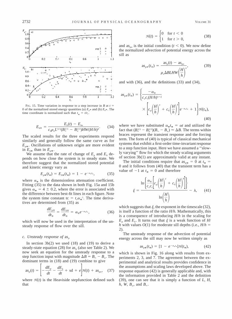
FIG. 15. Time variation in response to a step increase in B at t 50 of the normalized stored energy quantities (a) Ep* and (b) Ek*. Thetime coordinate is normalized such that t
*5 t/tr.
E (t) 2 Ek koE * 5 . (34)k 5/3 2/3 2/3 dc r L (B 2 B )HW(H/h)k o ` o
The scaled results for the three experiments respondsimilarly and generally follow the same curve as forEp*. Oscillations of unknown origin are more evidentin Ek* than in Ep*.
We assume that the rate of change of Ep and Ek de-pends on how close the system is to steady state. Wetherefore suggest that the normalized stored potentialand kinetic energy vary as
2a tE (t ) 5 E (t ) 5 1 2 e * *,p k* * * * (35)
where a* is the dimensionless attenuation coefficient.Fitting (35) to the data shown in both Fig. 15a and 15bgives a* 5 4 6 0.2, where the error is associated withthe difference between best-fit lines in each figure. Notethe system time constant tc 5 tr . The time deriva-21a*tives are determined from (35) as
dE * dE *p k 2a*t*5 5 a*e , (36)dt* dt*
which will now be used in the interpretation of the un-steady response of flow over the sill.
c. Unsteady response of asp
In section 3b(2) we used (18) and (19) to derive asteady-state equation (28) for asp (also see Table 2). Wenow seek an equation for the unsteady response to astep function input with magnitude DB 5 B` 2 Bo. Thedominant terms in (18) and (19) combine to give
dE dEp kas (t) 5 2 2 1 sd 1 e H (t) 1 as , (37)p po[ ]dt dt
where H (t) is the Heaviside stepfunction defined suchthat
0 for t , 0H (t) 5 (38)51 for t . 0,
and aspo is the initial condition (t , 0). We now definethe normalized advection of potential energy across thesill as
as (t) 2 asp poas *(t*) 5 , (39)p lHr DBLHWo 1 2h
and with (36), and the definitions (33) and (34),
2a*as *(t*) 5p l1j5c c (H/h)s t
g dH H2a*t*3 c 1 c e 1 1 H (t*),p k1 2 1 2 6[ ]h h
(40)
where we have substituted a*t* 5 at and utilized thefact that ( 2 )(B` 2 Bo) ø DB. The terms within2/3 2/3B B` o
braces represent the transient response and the forcingterm. The form of (40) is typical of classical mechanicalsystems that exhibit a first-order time-invariant responseto a step function input. Here we have assumed a ‘‘slow-ly varying’’ flow for which the steady scaling argumentsof section 3b(1) are approximately valid at any instant.
The initial conditions require that asp* 5 0 at t* 50 and it follows from (40) that the transient term has avalue of 21 at t* 5 0 and therefore
g da* H H
ln c 1 cp k5 1 2 1 2 6[ ]c c h hs t
j 5 2 l, (41)H
ln1 2h
which suggests that j, the exponent in the timescale (32),is itself a function of the ratio H/h. Mathematically, thisis a consequence of introducing H/h in the scaling forEp and Ek. It turns out that j is a weak function of H/h with values O(1) for moderate sill depths (i.e., H/h 52).
The unsteady response of the advection of potentialenergy across the sill may now be written simply as
2a tas (t ) 5 [1 2 e * *]H (t ),p* * * (42)
which is shown in Fig. 16 along with results from ex-periments 2, 3, and 7. The agreement between the ex-perimental and analytical results provides confidence inthe assumptions and scaling laws developed above. Theresponse equation (42) is generally applicable and, withthe information provided in Table 2 and the definition(39), one can see that it is simply a function of L, H,h, W, Bo, and B`.
SEPTEMBER 2001 2733F I N N I G A N E T A L .
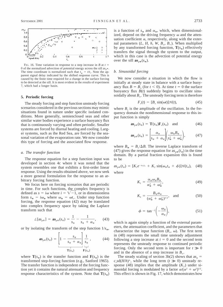
FIG. 16. Time variation in response to a step increase in B at t 50 of the normalized advection of potential energy across the sill asp*.The time coordinate is normalized such that t
*5 t/tt. Note the ap-
parent signal delay indicated by the shifted response curve. This iscaused by the finite time required for a change in the surface forcingto be detected at the sill. It is most evident in the results of experiment7, which had a longer basin.
5. Periodic forcing
The steady forcing and step function unsteady forcingscenarios considered in the previous sections may mimicsituations found in nature under specific isolated con-ditions. More generally, semienclosed seas and othersimilar water bodies experience a surface buoyancy fluxthat is continuously varying and often periodic. Smallersystems are forced by diurnal heating and cooling. Larg-er systems, such as the Red Sea, are forced by the sea-sonal variation of the evaporation rate. We now considerthis type of forcing and the associated flow response.
a. The transfer function
The response equation for a step function input wasdeveloped in section 4c where it was noted that thesystem resembles one that exhibits a first-order linearresponse. Using the results obtained above, we now seeka more general formulation for the response to an ar-bitrary forcing function.
We focus here on forcing scenarios that are periodicin time. For such functions, the complex frequency isdefined as s 5 iv where i 5 , or in dimensionlessÏ21form s* 5 iv* where v* 5 vtr. Under step functionforcing, the response equation (42) may be translatedinto complex frequency space by taking the Laplacetransform such that
1 1L [as *] 5 as *(s*) 5 2 , (43)p p s* s* 1 a*
or by isolating the transform of the step function 1/s*,
s* 1as *(s*) 5 1 2 , (44)p [ ]s* 1 a* s*
| | | |}}}}}}} }z z
T(s*) F(s*)
where T(s*) is the transfer function and F(s*) is thetransformed step-forcing function (e.g., Sanford 1965).The transfer function is independent of the forcing func-tion yet it contains the natural attenuation and frequencyresponse characteristics of the system. Note that T(s*)
is a function of s* and a*, which, when dimensional-ized, depend on the driving frequency v and the atten-uation coefficient a, respectively, along with the exter-nal parameters (L, H, h, W, Bo, B`). When multipliedby any transformed forcing function, T(s*) effectivelytransfers the signal through the system to the output,which in this case is the advection of potential energyover the sill asp*(s*).
b. Sinusoidal forcing
We now consider a situation in which the flow isinitially at steady state in balance with a surface buoy-ancy flux B 5 Bo (for t , 0). At time t 5 0 the surfacebuoyancy flux B(t) suddenly begins to oscillate sinu-soidally about Bo. The unsteady forcing term is therefore
F (t) 5 [B sin(vt)]H (t),s s (45)
where Bs is the amplitude of the oscillation. In the fre-quency domain the nondimensional response to this in-put function is simply
as *(s*) 5 T(s*)F (s*) and (46)p s
a* v*B*as *(s*) 5 , (47)p 2 21 2[ ]s* 1 a* s 1 v* *
where B* 5 Bs/DB. The inverse Laplace transform of(47) gives the response equation for asp*(t*) in the timedomain. By a partial fraction expansion this is foundto be
2a*t*as *(t*) 5 [K e 1 K sin(v*t* 1 f)]H (t*), (48)p 1 2
where
a*v*B*K 5 , (49)1 2 2a 1 v* *
B*a*K 5 , and (50)2 2 2 1/2(a 1 v )* *
v*21f 5 tan 2 , (51)1 2a*
which is again simply a function of the external param-eters, the attenuation coefficient, and the parameters thatcharacterize the input function (Bs, v). The first termin (48) represents the small time unsteady adjustmentfollowing a step increase at t 5 0 and the second termrepresents the unsteady response to continued periodicforcing. Only the second term is important for t k 0and in the absence of a step increase in Bo.
The steady scaling of section 3b(2) shows that asp 5cssd(H/h)l, while the long term (t k 0) unsteady re-sponse (48) implies that the amplitude (K2) under si-nusoidal forcing is modulated by a factor a/(a2 1 v2)1/2.This effect is shown in Fig. 17, which demonstrates how
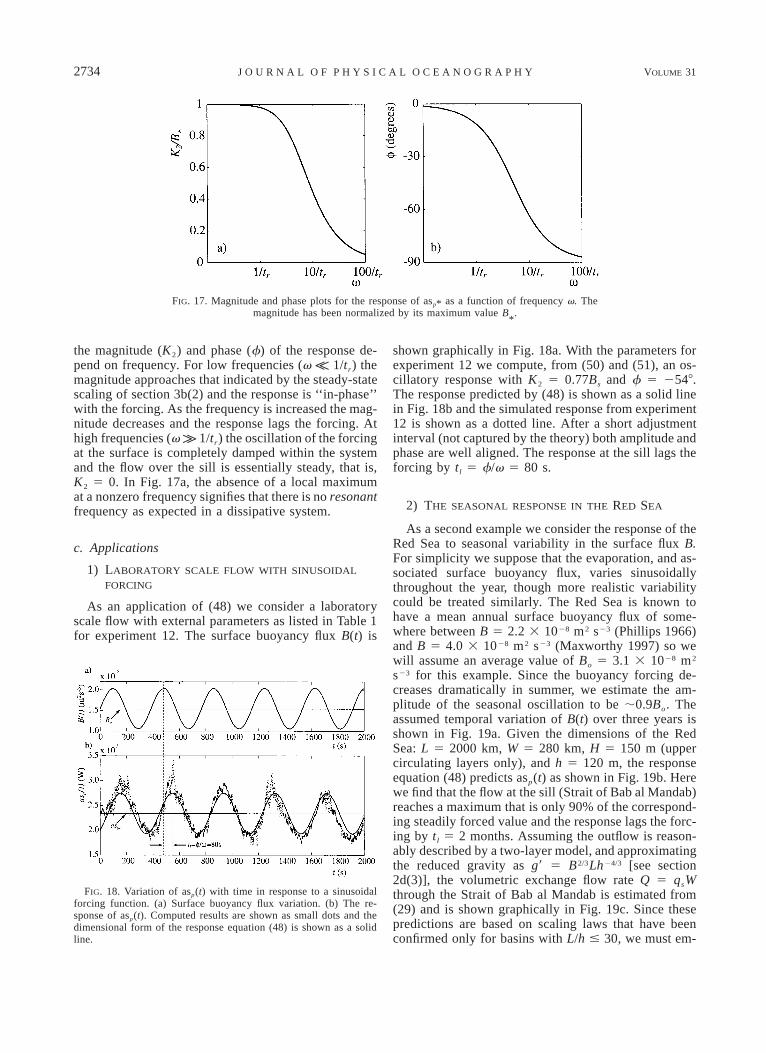
2734 VOLUME 31J O U R N A L O F P H Y S I C A L O C E A N O G R A P H Y
FIG. 17. Magnitude and phase plots for the response of asp* as a function of frequency v. Themagnitude has been normalized by its maximum value B
*.
FIG. 18. Variation of asp(t) with time in response to a sinusoidalforcing function. (a) Surface buoyancy flux variation. (b) The re-sponse of asp(t). Computed results are shown as small dots and thedimensional form of the response equation (48) is shown as a solidline.
the magnitude (K2) and phase (f) of the response de-pend on frequency. For low frequencies (v K 1/tr) themagnitude approaches that indicated by the steady-statescaling of section 3b(2) and the response is ‘‘in-phase’’with the forcing. As the frequency is increased the mag-nitude decreases and the response lags the forcing. Athigh frequencies (v k 1/tr) the oscillation of the forcingat the surface is completely damped within the systemand the flow over the sill is essentially steady, that is,K2 5 0. In Fig. 17a, the absence of a local maximumat a nonzero frequency signifies that there is no resonantfrequency as expected in a dissipative system.
c. Applications
1) LABORATORY SCALE FLOW WITH SINUSOIDAL
FORCING
As an application of (48) we consider a laboratoryscale flow with external parameters as listed in Table 1for experiment 12. The surface buoyancy flux B(t) is
shown graphically in Fig. 18a. With the parameters forexperiment 12 we compute, from (50) and (51), an os-cillatory response with K2 5 0.77Bs and f 5 2548.The response predicted by (48) is shown as a solid linein Fig. 18b and the simulated response from experiment12 is shown as a dotted line. After a short adjustmentinterval (not captured by the theory) both amplitude andphase are well aligned. The response at the sill lags theforcing by tl 5 f/v 5 80 s.
2) THE SEASONAL RESPONSE IN THE RED SEA
As a second example we consider the response of theRed Sea to seasonal variability in the surface flux B.For simplicity we suppose that the evaporation, and as-sociated surface buoyancy flux, varies sinusoidallythroughout the year, though more realistic variabilitycould be treated similarly. The Red Sea is known tohave a mean annual surface buoyancy flux of some-where between B 5 2.2 3 1028 m2 s23 (Phillips 1966)and B 5 4.0 3 1028 m2 s23 (Maxworthy 1997) so wewill assume an average value of Bo 5 3.1 3 1028 m2
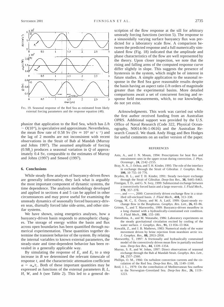
s23 for this example. Since the buoyancy forcing de-creases dramatically in summer, we estimate the am-plitude of the seasonal oscillation to be ;0.9Bo. Theassumed temporal variation of B(t) over three years isshown in Fig. 19a. Given the dimensions of the RedSea: L 5 2000 km, W 5 280 km, H 5 150 m (uppercirculating layers only), and h 5 120 m, the responseequation (48) predicts asp(t) as shown in Fig. 19b. Herewe find that the flow at the sill (Strait of Bab al Mandab)reaches a maximum that is only 90% of the correspond-ing steadily forced value and the response lags the forc-ing by tl 5 2 months. Assuming the outflow is reason-ably described by a two-layer model, and approximatingthe reduced gravity as g9 5 B2/3Lh24/3 [see section2d(3)], the volumetric exchange flow rate Q 5 qsWthrough the Strait of Bab al Mandab is estimated from(29) and is shown graphically in Fig. 19c. Since thesepredictions are based on scaling laws that have beenconfirmed only for basins with L/h # 30, we must em-
SEPTEMBER 2001 2735F I N N I G A N E T A L .
FIG. 19. Seasonal response of the Red Sea as estimated from likelyexternal forcing parameters and the response equation (48).
phasize that application to the Red Sea, which has L/h; O(104), is speculative and approximate. Nevertheless,the mean flow rate of 0.58 Sv (Sv [ 106 m3 s21) andthe lag of 2 months are not inconsistent with recentobservations in the Strait of Bab al Mandab (Murrayand Johns 1997). The assumed amplitude of forcing(0.9Bo) produces a seasonal variation in Q of approx-imately 0.4 Sv, comparable to the estimates of Murrayand Johns (1997) and Smeed (1997).
6. Conclusions
While steady flow analyses of buoyancy-driven flowsare generally informative, they lack what is arguablythe most important component of dynamic systems, thetime dependence. The analysis methodology developedand applied in sections 4 and 5 can be applied in othercircumstances and may prove useful for examining theunsteady dynamics of seasonally forced buoyancy-driv-en seas, diurnally forced lake side-arms, and other sim-ilar systems.
We have shown, using energetics analyses, how abuoyancy-driven basin responds to atmospheric chang-es. The storage of energy within the basin and fluxacross open boundaries has been quantified through nu-merical experimentation. These quantities together de-termine the transient behavior of the system. By relatingthe internal variables to known external parameters, thesteady-state and time-dependent behavior has been re-vealed in a generally applicable way.
By simulating the response of Ep and Ek to a stepincrease in B we determined the relevant timescale ofresponse tr and the characteristic attenuation coefficienta 5 a*/tr. Both of these important quantities may beexpressed as functions of the external parameters B, L,H, W, and h (see Table 2). This led to a general de-
scription of the flow response at the sill for arbitraryunsteady forcing functions (section 5). The response toa sinusoidally varying surface buoyancy flux was pre-dicted for a laboratory scale flow. A comparison be-tween the predicted response and a full numerically sim-ulated flow (Fig. 18) indicated that the amplitude andphase characteristics of the flow are well represented bythe theory. Upon closer inspection, we note that therising and falling arms of the computed response curvediffer slightly in slope. This suggests the presence ofhysteresis in the system, which might be of interest infuture studies. A simple application to the seasonal re-sponse in the Red Sea gave reasonable results despitethe basin having an aspect ratio L/h orders of magnitudegreater than the experimental basins. More detailedcomparisons await a set of concurrent forcing and re-sponse field measurements, which, to our knowledge,do not yet exist.
Acknowledgments. This work was carried out whilethe first author received funding from an AustralianOPRS. Additional support was provided by the U.S.Office of Naval Research (Code 322, Physical Ocean-ography, N0014-96-1-0616) and the Australian Re-search Council. We thank Andy Hogg and Ben Hodgesfor useful comments on an earlier version of the paper.
REFERENCES
Anis, A., and J. N. Moum, 1994: Prescriptions for heat flux andentrainment rates in the upper ocean during convection. J. Phys.Oceanogr., 24, 2142–2155.
Bray, N. A., J. Ochoa, and T. H. Kinder, 1995: The role of the interfacein exchange through the Strait of Gibraltar. J. Geophys. Res.,100, 10 755–10 776.
Bryden, H. L., and T. H. Kinder, 1991: Steady two-layer exchangethrough the Strait of Gibraltar. Deep-Sea Res., 38, S445–S463.
Finnigan, T. D., and G. N. Ivey, 1999: Submaximal exchange betweena convectively forced basin and a large reservoir. J. Fluid Mech.,378, 357–378.
——, and ——, 2000: Convectively driven exchange flow in a strat-ified sill-enclosed basin. J. Fluid Mech., 418, 313–338.
Gregg, M. C., E. Ozsoy, and M. A. Latif, 1999: Quasi-steady ex-change flow in the Bosphorus. Geophys. Res. Lett., 26, 83–86.
Grimm, T., and T. Maxworthy, 1999: Buoyancy-driven meanflow ina long channel with a hydraulically-constrained exit condition.J. Fluid Mech., 398, 155–180.
Harashima, A., and M. Watanabe, 1986: Laboratory experiments onthe steady gravitational circulation excited by cooling of thewater surface. J. Geophys. Res., 91, 13 056–13 064.
Kowalik, Z., and J. B. Mathews, 1983: Numerical study of the watermovement driven by brine rejection from nearshore arctic ice.J. Geophys. Res., 88, 2953–2958.
Maxworthy, T., 1997: A frictionally and hydraulically constrainedmodel of the convectively driven mean flow in partially enclosedseas. Deep-Sea Res., 44, 1339–1354.
Murray, S. P., and W. Johns, 1997: Direct observations of seasonalexchange through the Bab al Mandab Strait. Geophys. Res. Lett.,24, 2557–2560.
Phillips, O. M., 1966: On turbulent convection currents and the cir-culation of the Red Sea. Deep-Sea Res., 13, 1149–1160.
Reid, J. L., 1979: On the contribution of Mediterranean Sea outflowto the Norwegian–Greenland Sea. Deep-Sea Res., 26, 1119–1223.

2736 VOLUME 31J O U R N A L O F P H Y S I C A L O C E A N O G R A P H Y
Sanford, R. S., 1965: Physical Networks. Prentice-Hall, 576 pp.Smeed, D., 1997: Seasonal variation of the flow in the strait of Bab
al Mandab. Oceanol. Acta, 20, 773–781.Stommel, H., and H. G. Farmer, 1953: Control of salinity in an estuary
by a transition. J. Mar. Res., 12, 13–20.Sturman, J. J., and G. N. Ivey, 1998: Unsteady convective exchange
flows in cavities. J. Fluid Mech., 368, 127–153.
Winters, K. B., and H. Seim, 2000: The role of dissipation and mixingin an exchange flow through a contracting channel. J. Fluid.Mech., 407, 265–290.
——, ——, and T. D. Finnigan, 2000: Simulation of non-hydrostatic,density-stratified flow in irregular domains. Int. J. Numer. Meth-ods Fluids, 32, 263–284.