Embed Size (px)
Citation preview

RESOURCE USE AND CONSERVATION AND ENVIRONMENTAL IMPACTS IN THE
TRANSITION FROM CONFINEMENT TO PASTURE-BASED DAIRIES
By
M. Melissa Rojas-Downing
A THESIS
Submitted to
Michigan State University
in partial fulfillment of the requirements
for the degree of
Biosystems and Agricultural Engineering - Master of Science
2013

ABSTRACT
RESOURCE USE AND CONSERVATION AND ENVIRONMENTAL IMPACTS IN THE
TRANSITION FROM CONFINEMENT TO PASTURE-BASED DAIRIES
By
M. Melissa Rojas-Downing
In recent years, many farms have transitioned from total confinement housing to a pasture-based
system in an effort to reduce labor and production costs and improve profitability. There is a
growing interest in biogas recovery among livestock producers to reduce energy costs and
manure odors but the economic benefits of anaerobic digestion (AD) on small farms is not well
known. A comprehensive analysis was conducted using the Integrated Farm System Model, to
describe, evaluate and compare the economics, farm performance and environmental impacts of
representative dairy farms in Michigan transitioning from conventional confinement to a
seasonal- and pasture-based systems, and evaluate the potential for integration of an AD in the
confinement and seasonal pasture systems. In the economic analysis the annual pasture-based
system had the greatest net return to management and unpaid factors followed by the seasonal
pasture and confinement systems. The addition of an AD on a 100-cow, total confinement dairy
decreased the net return to management and unpaid factors by 15%. Cycling manure nutrients
led to an annual depletion of soil P and K on the confinement dairy and a build-up of P and K on
the seasonal- and pasture-based dairies. There was little change in N, P and K or carbon loss to
the environment due to AD. In the seasonal and annual pasture-based systems, ammonia
emissions increased by more than 100%. The water and reactive nitrogen footprint increased and
energy footprint decreased compared to the confinement dairy.

iii
My dedication is to my husband who with all his love, support, sacrifice, encouragement and
faith made the accomplishment of this thesis possible. With all my love this is for you.

iv
ACKNOWLEDGMENTS
I would like to express my sincere gratitude to my advisor Dr. Timothy Harrigan for all
the support, patience, motivation and knowledge during my Master’s program. I am thankful for
the opportunity provided to me by Dr. Harrigan and the Department of Biosystems and
Agricultural Engineering to obtain my degree. Besides my advisor, I would like to thank my co-
advisor Dr. Amirpouyan Nejadhashemi for all the continuous help, support and enthusiasm. I
have learned so much from both Dr. Harrigan and Dr. Nejadhashemi, and I am very grateful to
have had their guidance. I would like to extend my sincere thanks to my thesis committee
members, Dr. Steven Safferman and Dr. Santiago Utsumi, for their encouragement and insightful
comments. I would also like to thanks Dr. Katherine L. Gross, M.S. Mathew Haan, Jim Bronson,
Howard Straub, Dr. Dana Kirk and Dr. Alan Rotz for their technical knowledge and support
during the development of my research.
I would never have been able to finish my research without the help from the dairy
farmers who provided very useful information; the support from M.S. Faith Cullens and PhD
candidate Edwin Martinez (USDA-NRCS) who helped me connect with the farmers.
Furthermore, I would like to thank the Kellogg Biological Station, the Department of Biosystems
and Agricultural Engineering and the Merle and Catherine Esmay Scholarship for providing
financial support.
And last but not least, I would like to express my profound gratitude to my family and
friends who morally supported me and believed in me. My greatest appreciation is for my
husband for his support, advice, motivation, love, faith and patience in every moment of my
graduate study. This study would not have been possible without all of your help.

v
TABLE OF CONTENTS
LIST OF TABLES ......................................................................................................................... ix
LIST OF FIGURES ..................................................................................................................... xiv
KEY TO SYMBOLS AND ABBREVIATIONS ......................................................................... xv
CHAPTER 1: INTRODUCTION ................................................................................................... 1 1.1. Objectives ............................................................................................................................. 5
CHAPTER 2: LITERATURE REVIEW ........................................................................................ 6
2.1. Confinement Dairy Farms .................................................................................................... 7
2.2. Pasture-based Dairy Farms................................................................................................... 7 2.2.1. Characteristics of pasture-based dairy systems ............................................................. 9
2.3. Transition from confinement to a pasture-based dairy ....................................................... 10 2.4. Anaerobic Digestion ........................................................................................................... 11
2.4.1. Feedstocks for anaerobic digestion.............................................................................. 12 2.4.2. Byproducts ................................................................................................................... 14
2.4.2.1. Biogas .................................................................................................................. 14 2.4.2.1.1. Temperature .................................................................................................. 14 2.4.2.1.2. pH .................................................................................................................. 15
2.4.2.1.3. Retention Time.............................................................................................. 15 2.4.2.1.4. Solids concentration ...................................................................................... 16
2.4.2.1.5. Nutrient requirements and carbon/nitrogen ratio .......................................... 16 2.4.2.1.6. Mixing of the digesting material ................................................................... 17
2.4.2.1.7. Food to microorganism ratio ......................................................................... 18 2.4.2.1.8. Biogas use ..................................................................................................... 18
2.4.2.2. Digestate .............................................................................................................. 20 2.4.2.3. Reduce greenhouse gas emission ......................................................................... 22
2.4.3. Overall benefits and disadvantages of anaerobic digestion ......................................... 23
2.4.4. Types of Anaerobic Digester ....................................................................................... 24 2.4.4.1. Plug Flow Digester .............................................................................................. 26 2.4.4.2. Complete-mix Digester ........................................................................................ 26
2.4.4.3. Covered Lagoon ................................................................................................... 27 2.4.5. Dairy Manure Digester ................................................................................................ 27
2.4.5.1. Capital cost........................................................................................................... 30 2.4.5.2. Electricity ............................................................................................................. 35 2.4.5.3. Biomethane .......................................................................................................... 36 2.4.5.4. Heat ...................................................................................................................... 37 2.4.5.5. Digested solids ..................................................................................................... 37
2.4.5.6. Carbon-credits ...................................................................................................... 38 2.4.6. Regulations .................................................................................................................. 39
2.4.6.1. Federal Regulations related to Anaerobic Digestion ........................................... 40

vi
2.4.6.1.1. Air regulations .............................................................................................. 40
2.4.6.1.2. Solid Waste regulations ................................................................................ 41 2.4.6.1.3. Water regulations .......................................................................................... 41
2.4.6.2. Michigan permitting requirements related to Anaerobic Digestion .................... 41
2.4.6.2.1. Air permits .................................................................................................... 41 2.4.6.2.2. Solid waste permits ....................................................................................... 42 2.4.6.2.3. Water permits ................................................................................................ 42
2.5. Systems Modeling and Simulation ..................................................................................... 42 2.5.1. Crop models ................................................................................................................. 44
2.5.2. Farm economic models ................................................................................................ 45 2.5.3. Farm environmental and animal models ..................................................................... 45 2.5.4. Whole farm simulation models .................................................................................... 46 2.5.1. Integrated Farm System Model ................................................................................... 46
CHAPTER 3: PROCEDURE ....................................................................................................... 49
3.1. Representative farm development ...................................................................................... 52 3.1.1. Type of dairy farm ....................................................................................................... 52
3.1.2. Cattle frame ................................................................................................................. 53 3.1.3. Land base ..................................................................................................................... 54 3.1.4. Milk production ........................................................................................................... 54
3.1.5. Type of Manure Treatment .......................................................................................... 55 3.2. Herd and crop information of representative farms ........................................................... 63
3.3. Tillage and planting information ........................................................................................ 67 3.4. Economic information ........................................................................................................ 71 3.5. Pasture growth and management........................................................................................ 74
3.6. Crop nutrient requirements, nutrient availability and loss ................................................. 77
3.8. Anaerobic digestion............................................................................................................ 79 3.9. Environmental impacts ....................................................................................................... 82
CHAPTER 4. RESULTS AND DISCUSSION ............................................................................ 86 4.1. Comparison of farm performance and resource use........................................................... 86
4.1.1. Milk, feed and manure production .............................................................................. 87 4.2. Economics .......................................................................................................................... 90
4.2.1. Manure handling costs ................................................................................................. 91 4.2.2. Production costs ........................................................................................................... 93 4.2.3. Income and net return .................................................................................................. 96
4.3. Environmental impact ........................................................................................................ 98
4.3.1. On-farm nutrient cycling ............................................................................................. 98 4.3.2. Confinement systems ................................................................................................. 101
4.3.2.1. On-farm nutrient cycling .................................................................................... 101
4.3.2.1.1. Potassium .................................................................................................... 103 4.3.1.1.2. Nitrogen ...................................................................................................... 104 4.3.1.1.3. Phosphorus .................................................................................................. 104
4.3.2.2 .Environmental emissions ................................................................................... 105 4.3.2.2.1. Carbon dioxide and methane emissions ...................................................... 105

vii
4.3.2.2.2. Ammonia emissions .................................................................................... 107
4.3.2.2.3. Nitrous oxide emission ............................................................................... 108 4.3.2.2.4. Hydrogen sulfide emissions ........................................................................ 109
4.3.2.3. Environmental footprints ................................................................................... 110
4.3.2.3.1. Water footprint ............................................................................................ 111 4.3.2.3.2. Energy footprint .......................................................................................... 112 4.3.2.3.3. Reactive nitrogen loss footprint .................................................................. 113 4.3.2.3.4. Carbon footprint .......................................................................................... 114
4.3.3. Seasonal pasture farms .............................................................................................. 115
4.3.3.1. On-farm nutrient cycling .................................................................................... 115 4.3.3.1.1. Potassium .................................................................................................... 116 4.3.3.1.2. Nitrogen ...................................................................................................... 116 4.3.3.1.3. Phosphorous ................................................................................................ 119
4.3.3.2. Environmental emissions ................................................................................... 119 4.3.3.2.1. Carbon dioxide and methane emissions ...................................................... 120
4.3.3.2.2. Ammonia emissions .................................................................................... 121 4.3.3.2.3. Nitrous oxide emissions .............................................................................. 122
4.3.3.2.4. Hydrogen sulfide emissions ........................................................................ 123 4.3.3.3 Environmental footprints .................................................................................... 124
4.3.3.3.1. Water footprint ............................................................................................ 124
4.3.3.3.2. Energy footprint .......................................................................................... 125 4.3.3.3.3. Reactive nitrogen loss footprint .................................................................. 126
4.3.3.3.4. Carbon footprint .......................................................................................... 126 4.3.4. Annual Pasture-based farm ........................................................................................ 126
4.3.4.1. On-farm nutrient cycling .................................................................................... 126
4.3.4.1.1. Potassium .................................................................................................... 127
4.3.4.1.2. Nitrogen ...................................................................................................... 127 4.3.4.1.3. Phosphorous ................................................................................................ 127
4.3.4.2. Environmental emissions ................................................................................... 128
4.3.4.2.1. Carbon dioxide and methane emissions ...................................................... 128 4.3.4.2.2. Ammonia emissions .................................................................................... 129
4.3.4.2.3. Nitrous oxide emissions .............................................................................. 129 4.3.4.2.4. Hydrogen sulfide emissions ........................................................................ 129
4.3.4.3 Environmental footprints .................................................................................... 130 4.3.4.3.1. Water footprint ............................................................................................ 130 4.3.4.3.2. Energy footprint .......................................................................................... 130 4.3.4.3.3. Reactive nitrogen loss footprint .................................................................. 131
4.3.4.3.4. Carbon footprint .......................................................................................... 131
CHAPTER 5: CONCLUSIONS ................................................................................................. 132
CHAPTER 6: SUGGESTIONS FOR FUTURE RESEARCH ................................................... 136
APPENDICES ............................................................................................................................ 137

viii
APPENDIX A: DATA COLLECTED FROM FARM VISITS ON CONVENTIONAL
CONFINEMENT DAIRIES ................................................................................................... 138 APPENDIX B: DATA COLLECTED FROM FARM VISITS ON SEASONAL PASTURE
AND PASTURE-BASED DAIRIES ...................................................................................... 143
APPENDIX C: DATA SELECTED FOR THE FIVE REPRESENTATIVE DAIRY
PRODUCTION SYSTEMS .................................................................................................... 155 APPENDIX D: RESULTS FROM IFSM OF THE FIVE REPRESENTATIVE DAIRY
PRODUCTION SYSTEMS .................................................................................................... 172
REFERENCES ........................................................................................................................... 186

ix
LIST OF TABLES
Table 1. Estimated manure characteristics as excreted (ASABE, 2008) ...................................... 17
Table 2. Composition of Biogas from the Anaerobic Digestion of Dairy Manure....................... 19
Table 3. Summary of Characteristics of Digester Technologies (EPA, 2004) ............................. 25
Table 4. Summary of process attributes (Burke, 2001) ................................................................ 25
Table 5. Expected percentage VS conversion to gas (Burke, 2001) ............................................. 26
Table 6. Matching a Digester to a Dairy Facility (EPA-AgSTAR, 2004) .................................... 29
Table 7. Characteristics of lactating dairy cow manure and biogas potential (ASABE, 2005) .... 30
Table 8. Investment required for similar or any dairy operation with 160 milking cows (Lazarus,
2009) ............................................................................................................................................. 34
Table 9. Economic analysis of the digester (Lazarus, 2009) ........................................................ 35
Table 10. Estimated values for the seasonal pasture dairy with 142 medium-frame Holsteins,
anaerobic digestion, imported manure and additional land for cash crop production. ................. 59
Table 11.Major descriptive parameters of five representative dairy production systems ............ 64
Table 12. Major machines and structures used for planting and manure storage for five
representative dairy production systems ....................................................................................... 69
Table 13.Major machines and structures used for crop harvest and storage on the five
representative dairy production systems ....................................................................................... 71
Table 14. Major dairy costs ($/cow-year) ..................................................................................... 73
Table 15. Economic parameters and prices assumed for five representative dairy production
systems .......................................................................................................................................... 73
Table 16. Grazing parameters for the seasonal and annual pasture systems ................................ 76
Table 17. Anaerobic digester parameters ...................................................................................... 81

x
Table 18. Average annual milk, feed and manure production of five representative dairy
production systems........................................................................................................................ 88
Table 19. Manure handling costs ($/year) for five representative production systems ................ 92
Table 20. Total production costs ($/year) for five representative dairy production systems ....... 93
Table 21. Income and net return to management and unpaid factors ($/year) for five
representative dairy production systems ....................................................................................... 97
Table 22. Land area of five representative dairy production systems (ha) ................................. 101
Table 23. Annual nutrient cycling on five representative dairy farms. ...................................... 102
Table 24. Nutrient loss to the environment on five representative dairy farms (kg/ha-yr). ....... 102
Table 25. Environmental emissions of five representative dairy production systems ................ 105
Table 26. Biogenic carbon dioxide emissions of five representative dairy production systems
(kg/yr) ......................................................................................................................................... 106
Table 27. Methane emissions of five representative dairy production systems (kg/yr) ............. 107
Table 28. Ammonia emissions of five representative dairy production systems (kg/yr) ........... 108
Table 29. Nitrous oxide emissions of five representative dairy production systems (kg/yr) ..... 109
Table 30. Hydrogen sulfide emissions of five representative dairy production systems (kg/yr) 110
Table 31. Water footprints of five representative dairy production systems .............................. 111
Table 32. Energy footprint of five representative dairy production systems .............................. 112
Table 33. Reactive nitrogen loss footprint of five representative dairy production systems ...... 114
Table 34. Carbon footprint of five representative dairy production systems ............................. 115
Table A. 1. Land information collected from confinement farm…………………………... 139
Table A. 2. Crop information collected from confinement farm ................................................ 139
Table A. 3. Animal information collected from confinement farm ............................................ 139
Table A. 4. Livestock expenses information collected from confinement farm ......................... 140

xi
Table A. 5. Animal feeding information collected from confinement farm ............................... 140
Table A. 6. Animal facilities information collected from confinement farm ............................. 141
Table A. 7. Manure information collected from confinement farm ........................................... 141
Table A. 8. Storage structures information collected from confinement farm ........................... 142
Table B. 1. Land information collected from seasonal pasture and pasture-based farms…. 144
Table B. 2. Crop information collected from seasonal pasture and pasture-based farms ........... 145
Table B. 3. Animal information collected from seasonal pasture and pasture-based farms ....... 146
Table B. 4.Livestock expenses information collected from seasonal pasture and pasture-based
farms ........................................................................................................................................... 146
Table B. 5. Animal feeding information collected from seasonal pasture and pasture-based farms
..................................................................................................................................................... 147
Table B.6. Animal facilities information collected from seasonal pasture and pasture-based farms
..................................................................................................................................................... 148
Table B. 7. Manure information collected from seasonal pasture and pasture-based farms ...... 148
Table B. 8. Storage structures information collected from seasonal pasture and pasture-based 150
Table B. 9. Economic information collected from seasonal pasture and pasture-based farms .. 151
Table B. 10. Grazing information collected from seasonal pasture and pasture-based farms .... 152
Table B. 11. Data for calculations for fence investments ........................................................... 153
Table B. 12. Data for calculations for investment in watering system ....................................... 154
Table C. 1. Representative farms…………………………………………………………... 156
Table C. 2. Land information selected for farms F1, F2, F3, F4, F5, F6 .................................... 156
Table C. 3. Crop information for farms F1, F2, F3, F4, F5, F6 .................................................. 157
Table C. 4. Grazing information for farms F3, F4 and F5 .......................................................... 158
Table C. 5. Animal information for farms F1, F2, F3, F4, F5, F6 .............................................. 159
Table C. 6. Animal feeding information for farms F1, F2, F3, F4, F5, F6 ................................. 160
Table C. 7. Animal facilities information for farms F1, F2, F3, F4, F5, F6 ............................... 160

xii
Table C. 8. Manure information for farms F1, F2, F3, F4, F5, F6 ............................................. 161
Table C. 9. Storage structure information for farms F1, F2, F3, F4, F5, F6............................... 162
Table C. 10. Machine information for farms F1, F2, F3 and F4 ................................................ 163
Table C. 11. Machine information for farms F5 and F6 ............................................................. 164
Table C. 12. Miscellaneous information for farms F1, F2, F3 and F4 ....................................... 165
Table C. 13. Miscellaneous information for farms F5 and F6 .................................................... 166
Table C. 14. Tillage and planting information for farms F1, F2, F3, F4, F5, F6 ....................... 167
Table C. 15. Corn harvest information for farms F1, F2, F3, F4, F5, F6 ................................... 167
Table C. 16. Alfalfa harvest information for farms F1 and F2 ................................................... 168
Table C. 17. Alfalfa and grass harvest information for farms F3 and F4, F5 ............................. 169
Table C. 18. Alfalfa harvest information for farm F6................................................................. 170
Table C. 19. Hauling costs for imported manure in seasonal pasture system (F4) ..................... 171
Table D. 1. Development of seasonal pasture farm with 142 medium-frame Holsteins, cash crop,
imported manure and AD…………………………………………………...……………….173
Table D. 2. Average postharvest yield for crops of F1, F2, F3, F4, F5 ...................................... 176
Table D. 3. Annual feed production and utilization of F1, F2, F3, F4, F5 (Average) ................ 176
Table D. 4. Nutrients available, use and lost to the environment of F1, F2, F3, F4, F5 (Average)
..................................................................................................................................................... 177
Table D. 5. Annual manure production, nutrient availability and handling cost of F1, F2, F3, F4,
F5 (Average) ............................................................................................................................... 178
Table D. 6. Annual crop production, feeding costs and net return over those costs of F1, F2, F3,
F4, F5 (Average) ......................................................................................................................... 179
Table D. 7. Annual production costs and net return to management of F1, F2, F3, F4, F5
(Average) .................................................................................................................................... 180
Table D. 8.Crop production costs and feed costs of F1, F2, F3, F4, F5 (Average) .................... 181
Table D. 9. Annual emissions of important gaseous compounds of F1, F2, F3, F4, F5 (Average)
..................................................................................................................................................... 182

xiii
Table D. 10. Table of environmental footprints of water, nitrogen, energy and carbon for F1, F2,
F3, F4, F5 (Average) ................................................................................................................... 183

xiv
LIST OF FIGURES
Figure 1. Estimated potential of biogas production from manure co-digested with three different
percentages of feedstocks (Norman and Jianguo, 2004). ............................................................. 13
Figure 2. Estimated Annual Emission Reductions from Anaerobic Digestion (EPA, 2012b) ..... 23
Figure 3. Appropriate manure characteristics and handling systems for specific types of biogas
production systems (EPA-AgSTAR, 2004). ................................................................................. 28
Figure 4. Capital cost per dairy cow for complete mix, plug flow, and covered lagoon AD
systems (EPA-AgSTAR, 2010b) .................................................................................................. 31
Figure 5. Development of five representative dairy production systems ..................................... 58
Figure 6. Anaerobic Digestion in IFSM ....................................................................................... 79
Figure 7. Integrated Farm System Model Overview (USDA, 2013) ............................................ 99
Figure 8. Conceptual model of controls on N gas emissions from soil (modified from Parton et
al., 2001) ..................................................................................................................................... 100
Figure 9. Soil phosphorous and potassium build up and depletion ............................................ 103
Figure 10. Nutrients available on farm ....................................................................................... 117
Figure 11. Nutrients crop removal over that available on farm. ................................................. 117
Figure 12. Nitrogen lost to the environment of five representative dairy production systems ... 119
Figure 13. Ammonia emissions of five representative dairy production systems ...................... 121
Figure 14. Nitrous oxide emissions of five representative dairy production systems. ............... 122
Figure 15. Hydrogen sulfide emission of five representative dairy production systems. ........... 124
xv
KEY TO SYMBOLS AND ABBREVIATIONS
A Annual pasture-based farm
Ac Acres
AD Anaerobic Digester
ADIAC Anaerobic Digester Initiative Advisory Committee
ADIP Acid Detergent Insoluble Nitrogen
AEWR Adverse Effect Wage Rate
ALFALFA Integrative physiological model of alfalfa growth and development
ARS Agricultural Research Service- US Department of Agriculture
ASABE American Society of Agricultural and Biological Engineers
Avg. Average
BIOCOST Bioenergy crop costs
BOD Biologic Oxygen Demand
Btu British thermal unit
°C Celsius degrees
C Carbon
CAFOs Concentrated Animal Feeding Operations
CC Cash crop
CERES-Maize Crop Environment Resource Synthesis for corn

xvi
CFR Code of Federal Regulations
CH4 Methane
CO Carbon monoxide
CO2 Carbon dioxide
CO2e Carbon dioxide equivalent
COD Chemical Oxygen Demand
CP Crude protein
CS Cool season grass
ctw Hundredweight
CWT-EQ Hundredweight equivalent
DAFOSYM Dairy Forage System Model
DairyGem Dairy Gas Emissions Model
DGAS Dairy Greenhouse Gas Abatement Calculator
DHIA Dairy Herd Information Association
Dif. Difference
DM Dry matter
DNDC Denitrification-Decomposition model
em. Emission
EPA Environmental Protection Agency

xvii
EPIC Erosion-Productivity Impact Calculator
Ext. Extension
F Farm
FAO Food and Agricultural Organization
FARMSIM Farm Income Simulator
FPCM Fat and Protein Corrected Milk
ft Feet
gal Gallons
GHG Greenhouse Gas Emissions
GLYCIM Soybean Crop Simulator
Gov. Government
h Hours
H2 Hydrogen
H2O Water
H2S Hydrogen Sulfide
ha Hectares
hp Horse power
HRT Hydraulic Retention Time
IEA International Energy Agency

xviii
I-FARM Integrated crop and livestock production and biomass planning tool
IFSM Integrated Farm System Model
in Inches
IPCC Intergovernmental Panel on Climate Change
IRS Internal Revenue Service
K Potassium
kg Kilogram
kJ Kilojoule
km Kilometer
kW Kilowatt
L Legume
LAM Livestock Analysis Model
lb Pound
m3 Cubic meter
MBtu One thousand British thermal unit
Mcal Megacalorie
MDEQ Michigan Department of Environmental Quality
MI Michigan
min Minutes
MJ Megajule

xix
MMBtu Million British thermal unit
MSU Michigan State University
MUSLE Modified Universal Soil Loss Equation
MWh Megawatt hour
N Nitrogen
N2 Dinitrogen
NAASQS National Ambient Air Quality Standards
NASS National Agricultural Statistics Service
NDF Neutral Detergent Fiber
NFIFO Net Farm Income from Operations
NH3 Ammonia
NH3-N Ammoniacal Nitrogen
NH4+
Ammonium
NLEAP Nitrate Leaching and Economic Analysis Package
NMPs Nutrient Management Plans
NOx Nitrogen oxides
NPDES National Pollutant Discharge Elimination System
NRC National Research Council
NRCS Natural Resources Conservation Service - US Department of Agriculture

xx
P Phosphorous
PM Particulate Matter
ppm Parts per million
S Seasonal pasture farm
SRT Solids Retention Time
SWAT Solid and Water Assessment tool
t Metric tonne
TAN Total Ammoniacal Nitrogen
TS Total solids
U University
UDIM United Dairy Industry of Michigan
USDA United States Department of Agriculture
USDOE United States Department of Energy
VS Volatile solids
w With
yr Year

1
CHAPTER 1: INTRODUCTION
The United States has 51,481 dairy farms (Hoard’s Dairyman, 2012) and is the primary
milk producer in the world (Dairy Co, 2013). The U.S dairy industry is concentrated in the Great
Lakes region with 72% of the United States dairy farms in 2012 (Hoard’s Dairyman, 2012). This
region is well suited for dairying because forage is abundant and can be stored as winter feed
(EPA, 2012a). The Great Lakes region includes five of the top 10 milk producing states in 2012:
Wisconsin, New York, Pennsylvania, Minnesota and Michigan (NASS, 2013). The Michigan
dairy industry contributes $14.7 billion to the state economy (UDIM, 2013). According to the
USDA, 98% of United States dairy farms are family owned and operated, often by multiple
generations (UDIM, 2013).
In 2007 there were 9,158 million milk cows on 71,510 operations in the U.S. (Betts and
Ling, 2009). These cows produced 84.2 billion kilograms (185.6 billion pounds) of milk along
with an estimated 226.8 billion kilograms (500 billion pounds) of manure (Betts and Ling, 2009).
Manure processing is routinely handled by collecting, storing and spreading it over the land.
Manure contains several essential plant nutrients, such as nitrogen, phosphorous and potassium,
which, when is apply correctly, can replace commercial fertilizer applications and increase crop
yields. The type of manure and method of application (e.g. broadcast, injected) determine the
quantity of nutrient available to the plant (Pennington and VanDevender, undated).
There have been frequent complaints related to manure management, odor, and water
quality concerns, primarily directed at large livestock operations (Hadrich and Wolf, 2010).
Manure-related problems typically occur when liquid manure is spread during the late winter and
early spring when manure cannot be tilled in or adequately absorbed by the soil (EPA, 2011).
These environmental concerns along with other factors such as the reduction of land base on

2
which to apply manure, the increase in energy costs and growing interest in renewable energy
has encouraged farmers to search for alternative manure handling methods (Betts and Ling,
2009).
One of the alternatives that produce renewable energy in cost-effective ways is biogas
recovery system (U.S Department of Energy, 2012). The use of this technology has been
increasingly attractive for manure management with around 30 million anaerobic digesters
operating worldwide with manure (Chen et al., 2010). The Michigan Department of Labor and
Economic Growth states that this technology is gaining interest because of Michigan new laws
regulating odor, potential to reduce groundwater contamination and greenhouse gas production
in various parts of the United States (Simpkins, 2005). EPA estimated that there were 188
anaerobic digester operating at commercial livestock farms for biogas recovery in the United
States in 2012, and 158 were dairy digester projects (EPA, 2013).
The U.S. Environmental Protection Agency (EPA) in 2010 estimated 8,200 U.S. dairy
and swine operations produce more than 13 million MWh of electricity with biogas recovery
systems. Vanhorn et al. (1994) reported that dairy operations with less than 500 cows produce
3.4 million MWh annually. Anaerobic digesters allow compost and nutrient recovery. A
byproduct of biodigesters is a high quality organic fertilizer that can be used in cropping systems.
Odors associated with the land application of livestock waste are greatly reduced compared to
raw manure (Simpkins, 2005; Zhao et al., 2008). Most dairies that own or contribute manure to
biodigesters use the liquid effluent on their own fields (Lake-Brown, 2012). Anaerobic digestion
kills several pathogens and effectively reduces biological oxygen demand (BOD) and chemical
oxygen demand (COD) in waste, which protects surface waters when the effluent is land applied
(EPA, 2005).

3
The emission of CO2 and other greenhouse gases (GHG) has become an important issue.
Governments and industries are interested in technologies that will allow more efficient and cost-
effective waste treatment approaches which will minimize GHG production. Carbon credits will
promote the need for CO2 -neutral technologies (IEA Bioenergy, 2006). Anaerobic digestion
also impacts farm economics. EPA-AgSTAR (2010b) evaluated the capital costs of dairy farms
larger than 500 cows and compared common types of AD systems such as complete mix, plug
flow, and covered lagoon. The smallest farm was 500 cows and used a covered lagoon as an
anaerobic digester, with a capital cost of about $1600/per cow. A farm with 2,000 cows and a
covered lagoon had a capital cost of about $700/per cow and a farm with 4,000 cows and a plug
flow digester had a capital cost of about $750/per cow. One of the important factors that
influence the feasibility of setting up an anaerobic digester on a dairy production system is how
the managers utilize the byproducts (biogas and digestate) (Betts and Ling, 2009).
Perhaps the greatest operational challenge in integrating anaerobic digestion and pasture-
based dairies is the variable and seasonal supply of feedstock, and the lack of knowledge of how
to manage diverse feedstocks in the AD process. There is also a need for further research to
make anaerobic digestion byproducts more readily available, cost effective, and manageable to
small dairy facilities in the United States.
Researchers have created computer models that simulate crop growth, environment and
farming systems. Computer models allow the analyst to predict the effect of changes in complex
systems (Maria, 1997). Models can help stakeholders understand potential benefits, tradeoffs,
costs and impacts associated with management, environmental and other factors (Loucks and
Beek, 2005). A model should accurately represent the system and not be too difficult to

4
understand (Maria, 1997). The decision to include or assume information in the model requires
judgment, experience, and knowledge about the issues, the system being modeled and the
decision-making environment (Loucks and Beek, 2005).
The Integrated Farm System Model (IFSM) is a whole-farm simulation model that uses
historic weather data to determine long-term farm performance, environmental, and economic
impacts of dairy operations. The simulation includes all of the major processes involved in the
farming system including crop establishment, crop production, harvest, storage, feeding, milk
production, manure handling and the return of manure nutrients back to the land (Rotz et al,
2011a). Recently, a sub-model was added to include on-farm anaerobic digestion.
IFSM has been used to compare pasture-based with confinement system dairies. Rotz et
al. (2009) used IFSM to compare the predicted environmental impacts of four different dairy
operations in Pennsylvania where two of them were confinement dairies and two were rotational
grazing systems. They reported that the use of a grazing system could reduce erosion of
sediment, runoff of soluble P, the volatilization of ammonia, the net emission of greenhouse
gases and the C footprint. However, there is lack of information for evaluating the transition
from a confinement system to a pasture-based system, and the feasibility of anaerobic digestion
in such systems.
Rotz and Hafner (2011b) evaluated the addition of an anaerobic digester on a New York
state large confinement dairy farm (1,100 cows) over 25 years of weather. They used farm
records to validate simulated feed production and use, milk production, biogas production, and
electric generation and use. The digester reduced the net greenhouse gas emissions and farm gate
carbon footprint by 25 to 30% with a small increase in ammonia emission. There is a need to

5
evaluate the environmental and economic impact of the integration of an anaerobic digester on a
pasture-based system dairy farm with fewer than 500 cows.
Belflower et al (2012) evaluated the environmental impact of a management intensive
rotational grazing dairy and a confinement dairy in southeastern of United States. They reported
that ammonia emissions were higher on the confinement dairy due to manure handling.
Greenhouse gas emissions per cow were also higher on the confinement dairy, but the carbon
footprint from milk production on the pasture-based dairy was similar to the confinement system
which had greater milk production per cow. They concluded that well-managed pasture-based
dairy systems have environmental benefits due to reduced erosion and phosphorous runoff, and
reduced gas emissions from manure.
1.1. Objectives
A comprehensive analysis was conducted using Integrated Farming System Model
(IFSM) to evaluate resource use, economics and environmental impacts in the transition from a
100-cow, conventional confinement dairy to an annual pasture-based dairy. Specific objectives
were to:
1. Evaluate the operating costs and labor requirements of representative confinement-based
and seasonal-and pasture-based systems, including all major interactions from harvest
and feeding through manure application, tillage and planting.
2. Compare the economics and performance of an anaerobic digester on representative
confinement and seasonal pasture dairies.
3. Compare the environmental impacts of representative confinement, seasonal and annual
pasture-based dairies.

6
CHAPTER 2: LITERATURE REVIEW
In recent decades many U.S. dairy farms have increased their net income by expanding
herd size (Nott, 2003; USDA-NRCS, 2007). This increased the demand for feed and forage and
encouraged the use of confinement systems. Large confined herds required larger structures for
housing and feed storage and larger handling equipment and waste management systems
(USDA-NRCS, 2007).
A transition from confinement dairy to pasture-based dairy has been adopted due to the
profitability in the dairy industry in the Great Lakes Region (Nott, 2003). Pasture-based dairies
can reduce feed, labor, equipment and fuel costs. It provides a lower-cost option for small
farmers without expanding their dairy farm, or they can start dairying with less debt (USDA-
NRCS, 2007). Economic studies show that grazing farms can provide satisfactory profits
compared with confinement operations. Pasture-based systems generated $887 net farm income
from operations (NFIFO) per cow and $4.22 per hundredweight equivalent (CWT EQ),
compared to $640 NFIFO per cow and a negative $10 per CWT EQ (Kriegl and McNair, 2005).
From an environmental perspective, well-managed pasture-based dairies can reduce
erosion and protect water, air, plant and animal resources by maintaining vegetation over the
bare soil, increasing soil organic matter, improving water quality (because growing forages trap
sediments, fertilizer nutrients, pesticides, animal drugs and pathogens), improving the
distribution of nutrients on fields (because waste is more evenly spread) and reducing possible
odors, spills, or runoff from animal waste storage areas (USDA-NRCS, 2007; Purdue Extension,
undated extension bulletin).

7
2.1. Confinement Dairy Farms
USDA-NRCS (2007) defines a confinement-based dairy as one where land use and feed
management systems optimize milk production with confined cows consuming harvested
forages. In U.S. confinement dairies operations such as manure collection, storage, and land
application vary with farm size and cattle housing system (Gourley et al., 2011). Almost all the
herd is housed in a free stall or structure system with restricted or no access to pasture. Maternity
stalls and calf pens are typically housed in a shed, barn or hutch (Powell et al., 2005).
Confinement operations have more control of feed quantity and nutrient concentration
during the year which helps to stabilize milk production and nutrient concentrations in manure
(Wattiaux and Karg, 2004). Confinement farms tend to import more nutrients than needed by the
crops, and nutrient imbalance can result mainly when manure is applied in addition to fertilizer
applications in the absence of a regular soil testing program (USDA-NRCS, 2007).
2.2. Pasture-based Dairy Farms
USDA-NRCS (2007) defined a pasture-based dairy as a land use and feed management
system that optimizes the intake of forages consumed by grazing cows. USDA-NRCS (2007)
stated that pasture-based systems are based on two primary resources: pasture, which is a low-
cost feed (Soder and Rotz, 2001), and the dairy farmers management skills. Mechanical feed
harvesting and storage are reduced because the cow harvests the crop directly from the field.
Pasture-based dairies have several benefits. Less purchased feed is required; therefore,
fewer acres need to be harvested as stored forage. Producers can also extend the grazing season
to fall, winter or spring by using different forage crops (USDA-NRCS, 2007).
Typically, in a pasture-based system, forage reaches the rumen as high quality feed
(USDA-NRCS, 2007). Vegetative forage is higher in available protein, energy, and essential

8
nutrients than stored forage. Vegetative forage is better than mature grass because grasses tend to
build up thicker cell walls once they mature, meaning there are fewer nutrients available for the
livestock (Purdue Extension, undated extension bulletin).
Seventy to eighty percent of nutrients of consumed feed and forage is returned to land
(Whitehead, 1995). The dairy cattle diet, such as supplemental forages and concentrates, needs to
maintain a balance of nutrients going out through milk production to reduce fertilizer
applications. This maintains fertility levels in the cropland by replacing, with manure or
inorganic fertilizer, the nutrients that leave the field in the harvested crop. Between 70 and 90
percent of the phosphorus, potassium, calcium and magnesium consumed by dairy cattle are
excreted back onto the pasture (Mott, 1974).
Healthier cows with longer productive lives are common on pasture-based dairies.
Grazing reduces foot and hoof problems, increases calving percentage, reduces parasite
problems, and reduces fly problems (Purdue Extension, undated extension bulletin). Because
cows tend to live longer less money is spent on replacement animals and more income is realized
from selling heifers (Kriegl and McNair, 2005).
Grazing reduces manure handling and odors produced by concentrated manure areas
because animals tend to herd less. In pastures, decomposition of manure and undigested feed
occurs faster due to the aerobic conditions. In confinement systems, accumulated wet waste can
increase the odor problem and ammonia volatilization (Tyrell, 2002).
There are many ways to graze, but some of the basic methods include continuous grazing,
rotational grazing and management-intensive grazing. In continuous grazing, animals graze in a
single large area for the entire season. This is the simplest form of grazing for the farmer in terms
of costs and labor. However, this management practice is associated with low forage quality and

9
yield, lower stocking rate, overgrazing and uneven manure distribution (Purdue Extension,
undated extension bulletin).
Rotational grazing uses more than one pasture so grazing animals can be moved from one
pasture to another based on their feed requirements and forage growth. This allows pastures to
rest and re-grow, distributes manure more evenly, and increases forage production. The costs of
this system are higher than continuous grazing because of the need for water distribution and
fencing (Purdue Extension, undated extension bulletin).
Management-intensive grazing divides large fields into smaller paddocks so animals can
be moved frequently at high stocking rates thereby providing as much of the needed forage as
possible from pasture. This type of grazing systems provides the greatest forage production per
area, controls weeds and brush naturally, provides the most even manure distribution, gives more
forage options, and allows paddocks to rest and regrow completely. The disadvantages are that it
requires careful monitoring and greater startup cost for water distribution and fencing (Purdue
Extension, undated extension bulletin).
2.2.1. Characteristics of pasture-based dairy systems
USDA-NRCS (2007) described the characteristics for an efficient and productive pasture-
based dairy system based on practices that optimize livestock performance, pasture quality and
dry matter yield and the efficiency of forage utilization.
In pasture-based systems, lactating animals are pastured in a way that the entire herd
grazes a fresh paddock on alternating days leaving sufficient forage. The animals are on pasture
at least 75% of the grazing season and dry cows and heifers are 90%. Lactating animals obtain
around 50% of their forage intake during the grazing season and dry cows and heifers obtain
around 90%.

10
Every rotation cycle paddocks will vary in size to provide sufficient forage for adequate
livestock intake and forage residual to maintain pasture growth. A back fence limits access to the
paddocks that where recently grazed by the cows, while a front fence limits the availability of
fresh and ungrazed grass. Lanes allow movement between the milk parlor and paddock. Cattle
will have available water inside the paddock or in the lane near the paddock in which they are
grazing. On average, a cow requires 2 to 2.3 kilograms (4.5 to 5 pounds) of water per day per
pound of milk produced (Purdue Extension, undated extension bulletin).
A usual rule of thumb is that at least 0.40 ha (one acre) of pasture is necessary for each
lactating cow and this area should be within 1.6 km of the milking facility during warm weather.
Usually, forage yield will limit herd size (USDA-NRCS, 2007).
There are several indicators for assessing the economic success of various systems, but
the best indicator is net farm income from operations (NFIFO) per cow or net cost of production
per hundred-weight (CWT) of milk produced (USDA-NRCS, 2007). There are some cases where
dairy herds exceed 9,072 kilograms (20,000 pounds) of milk per cow per year, and some
producers have reported herd averages of 10,866 to 11,784 kilograms (24,000 to 26,000 pounds)
of milk per cow per year. However, some pasture-based dairy herds are cost-effective producing
6,804 kilograms (15,000 pounds) of milk per cow per year (USDA-NRCS, 2007). Some
obstacles are the types or characteristics of the climate or land base (rough, fragmented terrain,
wet soils, heat and humidity or cold weather), which can prevent efficient grazing of dairy cows.
2.3. Transition from confinement to a pasture-based dairy
In the transition period from a confinement to pasture-based dairy it is important to take
into account all aspects of the major shifts in production and operations. Some of the changes
needed to increase efficiency are to improve the milking facilities to reduce milking time;

11
improve pasture fertilization by soil testing and applying recommended fertilizer rates; reduce
expensive farm machinery investments; and during the grazing season feed pasture forage based
on cattle dry matter intake, amount of standing forage within the paddock, and on forage
nutrients (USDA-NRCS, 2007).
During the transition from confinement to pasture system there will be a temporary loss
of milk production (Kriegl and McNair, 2005) because cows that have never grazed before
expect feed that is provided in the barn and they may not know that they will need to graze to
obtain feed. However, milk production will increase and meet or exceed their level of production
when the cows have learned to graze and maximize dry matter intake from pasture (Purdue
Extension, undated extension bulletin).
The onset of cold temperatures decreases the forage available for grazing; therefore, more
feed needs to be supplemented in the barn and cows need to adjust to eat these feeds again. In
general, cows are kept in the barn when nighttime temperatures consistently fall below 4.4
degrees Celsius (40 Fahrenheit). However, if there is forage available, the cows can graze during
the day. There are also some farmers that are experimenting with “outwintering” their cattle. In
this case, cows would be left out at night to adapt to the colder temperatures and the feed is
brought to them (Purdue Extension, undated extension bulletin).
2.4. Anaerobic Digestion
Anaerobic digestion (AD) is a process where anaerobic bacteria degrade organic
materials in an oxygen free environment to create biogas (mix of methane and carbon dioxide),
which can be used to produce electricity and heat (Burke, 2001). The use of anaerobic digesters
in the U.S started during 1970’s energy crisis. In 1972, a farm near the town Mt. Pleasant, Iowa,
was one of the first farms of U.S. to install an anaerobic digester (Mattocks and Wilson, 2005).

12
Because of federal incentives, by the 1980’s there were already 120 agricultural digesters (Center
for Climate and Energy Solutions, 2011), but economic issues and technical problems led to a
60% failure rate of those digesters (Bishop and Shumway, 2009). In recent years, new incentives
(grants and loan guarantees) and policies (in the form of renewable electricity standards) have
helped increase the use of agricultural anaerobic digesters. EPA-AgSTAR (2011b) estimated 176
digesters were in operation in the United States for livestock manure and many of them were
new. The number of digesters in use has been increasing gradually for more than a decade with
an average of 16 new digesters each year (AgSTAR, 2011b).
2.4.1. Feedstocks for anaerobic digestion
The input for an anaerobic digester is biomass, such as manure, agricultural waste, and
urban waste, though they are not similarly degraded or converted to gas (Burke, 2001). Co-
digestion uses a mix of different feedstocks. The use of animal manure as a feedstock for AD is
widespread because it produces a valuable fertilizer as well as biogas (IEA Bioenergy, 2006).
Flowing, uniform manure slurry collected daily on a regular schedule is ideal, but pre-treatment
may be required to adjust the amount of solids in the manure to meet the requirements of the
digester (Betts and Ling, 2009).
Digestion transforms the content of manure. There are small reductions in the total of
volume of manure due to saturation of the biogas leaving the reactor with water vapor, but this
reduction is negligible (EPA-AgSTAR, 2011a). What make digesters helpful are the changes in
manure properties and solids separation (Simpkins, 2005). This reduces undesirable odors
(Simpkins, 2005) and most nutrients are transformed from an organic form to an inorganic form.
The nutrients in manure improve crop yields by converting nitrogen to ammonium, a more
readily available form for plant uptake (Betts and Ling, 2009; Lansing et al., 2008). Some studies

13
have shown that crop yields are equivalent to but not greater than those with non-digested
manure (Allan et al., 2003; Möller and Müller, 2012).
Instead of using only one type of biomass a mix of different types of biomass can be
used. An advantage of co-digestion is an increase in different types of feedstocks that can be
used for stakeholders that want to increase their biogas yield (The Minnesota Project, 2010).
Although animal manure is a very well-known feedstock for anaerobic digesters, it produces a
small amount of biogas per kilogram of biomass compared to other type of feedstocks (Biogas
Energy Inc, 2008 ). The main problem with co-digestion is creating the right mix of feedstock
based on availability and location so that the cost of transport of the feedstock is not higher that
the profits due to the co-digestion (The Minnesota Project, 2010).
Typical dairy waste biogas is 55 to 65% methane and 35 to 45% carbon dioxide with
some trace quantities of hydrogen sulfide and nitrogen (Burke, 2001). If animal waste and other
organic feedstock are combined in the right way biogas production may increase anywhere from
200 to 500% (El-Mashad and Zhang, 2007). Figure 1 shows the estimated potential of biogas
production from manure co-digested with three different percentages of feedstocks.
Figure 1. Estimated potential of biogas production from manure co-digested with three different
percentages of feedstocks (Norman and Jianguo, 2004).
0
1
2
3
4
5
6
7
Bio
gas
pote
nti
al
(m3/c
ow
/day
)
100% manure
75% manure and
25% food waste
50% manure and
50% food waste

14
An additional benefit of co-digestion of organic wastes is that with the right combination
of different organic wastes the amount of nutrients in the digestate can be optimized to create an
effective fertilizer (EPA, 2005).
2.4.2. Byproducts
Outputs of anaerobic digestion are biogas and digestate. Biogas is available to heat the
digester and potentially satisfy other farm energy needs and sometimes provide energy for
export. Another byproduct is the digestate which can be divided into solid and liquid components
using a separator and can be used as a fertilizer (Burke, 2001).
2.4.2.1. Biogas
The environment in the digester and the feedstock characteristics will affect the rate of
conversion of biomass to biogas (Betts and Ling, 2009). Several factors can affect the rate of
digestion and biogas production including temperature, pH, retention time, solids concentration,
nutrient levels and carbon/nitrogen ratio, food to microorganism ratio, mixing of the digesting
material and the particle size of the material being digested (Burke, 2001).
2.4.2.1.1. Temperature
In terms of overall system cost and reliability, medium-high temperatures are best
(mesophilic temperature range 35°C- 40.5°C) (Simpkins, 2005). The mesophilic process is more
tolerant to changes in feed materials or temperature. In the thermophilic range (50°C - 60°C)
decomposition and biogas production occurs faster than in the mesophilic range but the process
is less tolerant of changes. Biodigester temperature must be kept constant to optimize the
digestion process (U.S Department of Energy, 2012).
The U.S Department of Energy (2012) reported that anaerobic bacteria can tolerate
temperatures from below freezing to more than 57.2°C. Because methane bacteria are naturally

15
widespread in the environment, anaerobic degradation can be achieved at moisture contents from
around 50% to more than 99% but they operate best at temperatures of about 36.7°C
(mesophilic) and 54.4°C (thermophilic) (IEA Bioenergy, 2006).
2.4.2.1.2. pH
The importance of pH in a digester is that it maintains the production and balance of
methanogenic and acetogenic, or acetate-producing organisms. Chynoweth and Isaacson (1987)
reported that the optimal pH for anaerobic digestion was between 7.0 and 8.0. The pH of manure
is at 7.0 or slightly above (USDA, 2003). Methanogenic microorganisms require a pH between
6.8 and 8.5 to produce methane (Burke, 2001).
Acid forming bacteria typically grow more rapidly than methane forming bacteria,
creating an excess of acid (low pH) in the system and inhibiting the activity of methane forming
bacteria. Methane production may stop completely, but if it is maintained a large amount of
methane producing bacteria these pH instability could be prevented (Burke, 2001).
2.4.2.1.3. Retention Time
Retention time determines reactor volume and maintenance of biological reactions.
Hydraulic retention time (HRT) is the time a volume of influent remains in a digester. Solids
retention time (SRT) is the length of time solids spend inside a digester and is the most important
factor regulating the conversion of solids to gas and maintenance of digester stability (Burke,
2001).
Volatile solids (VS) are the basis for estimating organic composition and determining
retention times. The degradation of VS in manure increases logarithmically with SRTs greater

16
than approximately 10 days. After approximately 30 days, VS destruction increases linearly until
a maximum of 65 percent VS conversion to gas is achieved (Burke, 2001).
The SRT and HRT are equal when the digesters do not have digestate solid/liquid
separation, followed by recirculation (Burke, 2001). If the SRT is too low, the rate of microbial
loss exceeds the rate of growth, causing a “wash out” and a low level of biogas production
(Burke, 2001). If the SRT is high the AD must have a larger digester volume, increasing the
ability to dilute toxic compounds and allowing more time for microbes to adapt to toxic
compounds (Gerardi, 2003).
2.4.2.1.4. Solids concentration
Biogas production depends on the solids concentration of the feedstock when the digester
is operating close to the optimum retention time (Wheatley, 1990). Lower VS concentrations
require a longer SRT for effective biogas production (Chynoweth and Isaacson, 1987). Water
content of raw biomass must be measured constantly because digestion of material with total
solid content lower than 5% is usually not feasible (EPA, 2005) but some dilution can have
positive effects. Water can dilute the concentration of some components such as nitrogen and
sulfur from which ammonia and hydrogen sulfide can be produced and inhibit the anaerobic
digestion process (Burke, 2001).
2.4.2.1.5. Nutrient requirements and carbon/nitrogen ratio
Carbon (C), nitrogen (N), and phosphorus (P) are macronutrients present in dairy cattle
manure needed for production of methanogens. ASABE (2008) presents typical macronutrient
values for as-excreted dairy lactating cow manure (Table 1). Chen and Hashimoto (1978)
reported an optimal C to N ratio of 23:1 for methane forming microorganisms and Archer (1985)

17
reported an optimal C to P ratio of 100-150:1. Iron, nickel, and sulfur, used in the reaction of
acetate to methane, are the most important micronutrients required for production of
methanogenic microorganisms. Other nutrients of importance needed in limited quantities, are
selenium, barium, calcium, magnesium and sodium (Gerardi, 2003).
Table 1. Estimated manure characteristics as excreted (ASABE, 2008)
Characteristic Dairy Lactating Cow Units
Total solids 8.9 kg / day
Volatile solids 7.5 kg / day
COD 8.1 kg / day
BOD 1.3 kg / day
Nitrogen 0.45 kg / day
P 0.078 kg / day
K 0.103 kg / day
Total Manure 68 kg / day
Total Manure 68 liter / day
Moisture 87 % w.b.
2.4.2.1.6. Mixing of the digesting material
Mixing of the biomass during the digestion process can aid biogas production (U.S
Department of Energy, 2012). Bedding mixed with manure can inhibit anaerobic digestion by
reducing biogas production potential. Bedding increases bulk densities within digesters with
materials that do not digest very well. The mass transfer within the digester will decrease and
required mixing energies will increase, both of which reduce the overall performance of the
digester (Arora, 2011). Sands and silts cause problems by clogging pipes, damaging equipment,
and accumulating in anaerobic digestion tanks (Burke, 2001). The exception is at low
concentrations in a well-mixed digester where the mixing keeps sand in suspension
(Burke, 2001), even though the mixer takes up space and increases energy cost (Safferman,
personal communication, 2013).

18
2.4.2.1.7. Food to microorganism ratio
Food-to-microorganism ratio (F: M) is important because it controls anaerobic digestion.
The food-to-microorganism ratio (F: M) is the ratio of kilograms of waste supplied to the
kilograms of bacteria available to consume the waste. Depending on temperature, bacteria will
consume a limited amount of food per day, so one must supply the proper amount of bacteria to
consume the required amount of waste. A lower F: M ratio will convert more quantity of waste
to gas (Burke, 2001).
2.4.2.1.8. Biogas use
Biogas can be used as a high quality natural gas or as an alternative fuel in engines to
generate electricity, boilers to produce hot water and steam, and gas fired absorption chillers
used for refrigeration (USDOE, 1996).
Gas collected from anaerobic digestion is a combination of methane (CH4), carbon
dioxide (CO2), and trace amounts of other gases such as water vapor and hydrogen sulfide (H2S)
(Walsh et al., 1988). The typical combination of biogas from a digester with dairy manure is
listed in Table 2. Biogas properties influence the choice of technologies for cleaning and
utilizing biogas (Yadav et al., 2013).

19
Table 2. Composition of Biogas from the Anaerobic Digestion of Dairy Manure
Typical (Percent by volume)
Methane CH4 60-70
Carbon Dioxide CO2 30-40
Hydrogen Sulfide H2S 300-4,500 ppm
Ammonia NH3 Trace
Hydrogen (H2) Trace
Nitrogen gas (N2) Trace
Carbon Monoxide (CO) Trace
Moisture (H2O) Trace
Other* Trace
* Particles, Halogenated hydrocarbons, Nitrogen, Oxygen, Organic silicon compounds, and
others (USADA-NCRS, 2009)
Each liter of waste processed will produce a quantity of energy depending on the percent
conversion of volatile solids to gas. Volatile solids destruction results in methane generation.
Each kilogram of volatile solids produces 0.36 cubic meter of methane. Each 0.03 cubic meter
(one cubic foot) of methane can produce1055 KJ (1000 Btu) of energy. Therefore, 0.45
kilograms (one pound) of volatile solids will produce 5929 KJ (5620 Btu) of energy. At 35
percent conversion efficiency, the 0.45 kilograms (one pound) of volatile solids will produce
0.58 kWh of energy (Burke, 2001). Biogas can also be used for producing electricity through an
internal combustion engine or gas turbine. The engine used produces waste heat (more than
60%) which can be used for heating the facilities, hot water and the digester (EPA, 2005). This
generation of heat and power is known as “cogeneration”, which is created from biogas (Betts
and Ling, 2009).
The biogas can be flared or burned off, but the only advantage is that it breaks down the
methane through combustion, reducing methane emissions (Betts and Ling, 2009). However, this
option for biogas does not produce revenue for the farm (Binkley, 2010).

20
2.4.2.2. Digestate
The non-gaseous material remaining after digestion is referred to as digestate (USDOE,
1996) and can be separated into solid and liquid fractions. Benefits of separating the solids and
liquids from digestate include the recovery of bedding, decrease in volume of liquid manure
storage, and the ability to sell solid digestate as fertilizer (Sheffield, 2008). The increase in
temperature during the digestion process reduces pathogens that are found in waste that
accumulates in waste storage facilities (The Minnesota Project, 2010).
Solid and liquid components of the digestate can be used as a fertilizer. In the solid
portion of digestate most of the P remains and is sold as bulk fertilizer. The liquid portion retains
much of the N that is largely converted to ammonium, which is the main component in
commercial based fertilizers (The Minnesota Project, 2010). Both can be land applied, thereby
offsetting commercial fertilizer purchases.
Manure from AD seems to reduce phosphorus and micronutrients that are available for
plants, but there is no apparent effect on the short-term crop availability under field conditions.
Möller and Müller (2012) showed that adding crop and cover crops residues to the anaerobic
digestion process increased the total amounts of mobile organic nutrients within the farming
system while nitrogen use efficiency was also higher.
It is common to use post-digestion solid waste as bedding for animals on the farm
because it eliminates most, if not all, of the bedding costs. Most farmers that had used solid
digestate as bedding report that is great for cow well-being and is also known to be less
vulnerable to disease spreading bacteria, because the digestion process removes most of the
digestible organic matter (EPA, 2005).

21
Another benefit of the digestate is odor reduction. Anaerobic digesters can reduce manure
odors by 70% to 80% compared to untreated manure (Zhao et al., 2008). Two of the three stages
of biogas production are related to odor. During the first stage there can be some undigested
materials because some fibrous material cannot be liquefied and other inorganic materials can
either accumulate or pass through the digester intact. Undigested materials make up the low-odor
in the digestate (Legget et al., undated).
In typical liquid manure storage more acid forming bacteria can survive than methane
forming bacteria (because of their sensitiveness to the environment), producing more acids that
are not converted to biogas. This excess of volatile acids produces a putrid odor (Legget et al.,
undated). In contrast, during the second stage of the anaerobic digestion process more acids are
converted to biogas thereby reducing odor.
Digestate can have some changes in composition during the digestion process. One of
them is a reduction in solids content, which for manure slurry could be up to 25% with an
increase in ash content, because of mineral conservation, decrease of slurry carbon and decrease
of organic matter content. However, due to variability in feedstock and digester conditions, the
changes can be inconsistent (Scottish Executive Environment and Rural Affairs Department,
2007). There is also an increase in slurry pH (up to 0.5) and ammonium nitrogen content (up to
25%) (Scottish Executive Environment and Rural Affairs Department, 2007).
The increase in slurry ammonium-N content could have some environmental impact by
increasing emissions of ammonia during post-digestion storage, which could be controlled with
storage covers and following application of the digestate on the land. The reduced solids content
could improve surface infiltration of the digestate, which could help to conserve nitrogen
(Scottish Executive Environment and Rural Affairs Department, 2007).

22
2.4.2.3. Reduce greenhouse gas emission
Anaerobic digesters reduce greenhouse gas emission reductions in two ways:
1. The capture and burning of biogas reduces methane emission which else would be
released into the atmosphere from the waste management system (ADIAC, 2009).
2. Fossil fuels are displaced due to the use of biogas to generate energy, therefore
greenhouse gases emissions (CO2, methane, and nitrous oxide) and other pollutants
are avoided (ADIAC, 2009).
The overall impact of converting CH4 to CO2 is beneficial. Methane from a digester is
destroyed through combustion, and combustion produces CO2 and H2O. Methane is around 25
times more damaging than CO2 in its effect on global warming (IPCC, 2007).
EPA (2012b) presents a graph (Figure 2), which shows the annual emission reductions,
including both direct reductions and avoided emissions, due to anaerobic digesters since 2000. In
total, the combustion of biogas at the digesters prevents the direct emission of about 61,000
metric tons of methane annually (1,278,000 metric tons of CO2 equivalent) (EPA, 2012b).

23
Figure 2. Estimated Annual Emission Reductions from Anaerobic Digestion (EPA, 2012b). For
interpretation of the references to color in this and all other figures, the reader is referred to the
electronic version of this thesis.
2.4.3. Overall benefits and disadvantages of anaerobic digestion
Anaerobic digestion is a natural waste treatment process. It reduces disposed waste
volume to be landfilled and it requires less land than aerobic composting (IEA Bioenergy, 2006).
EPA (2012b) made a comparison of organic food scrap recycling technologies for a facility
processing 40,000 tons per year of organic materials. Anaerobic composting required between
2.4 to 5.3 ha of land area and anaerobic digestion required 1.2 to 2.4 ha.
Anaerobic digestion is an energized process. Biogas is used for heat or electrical
generation. Waste heat can be used for heating and cooling dairy facilities. The power generated
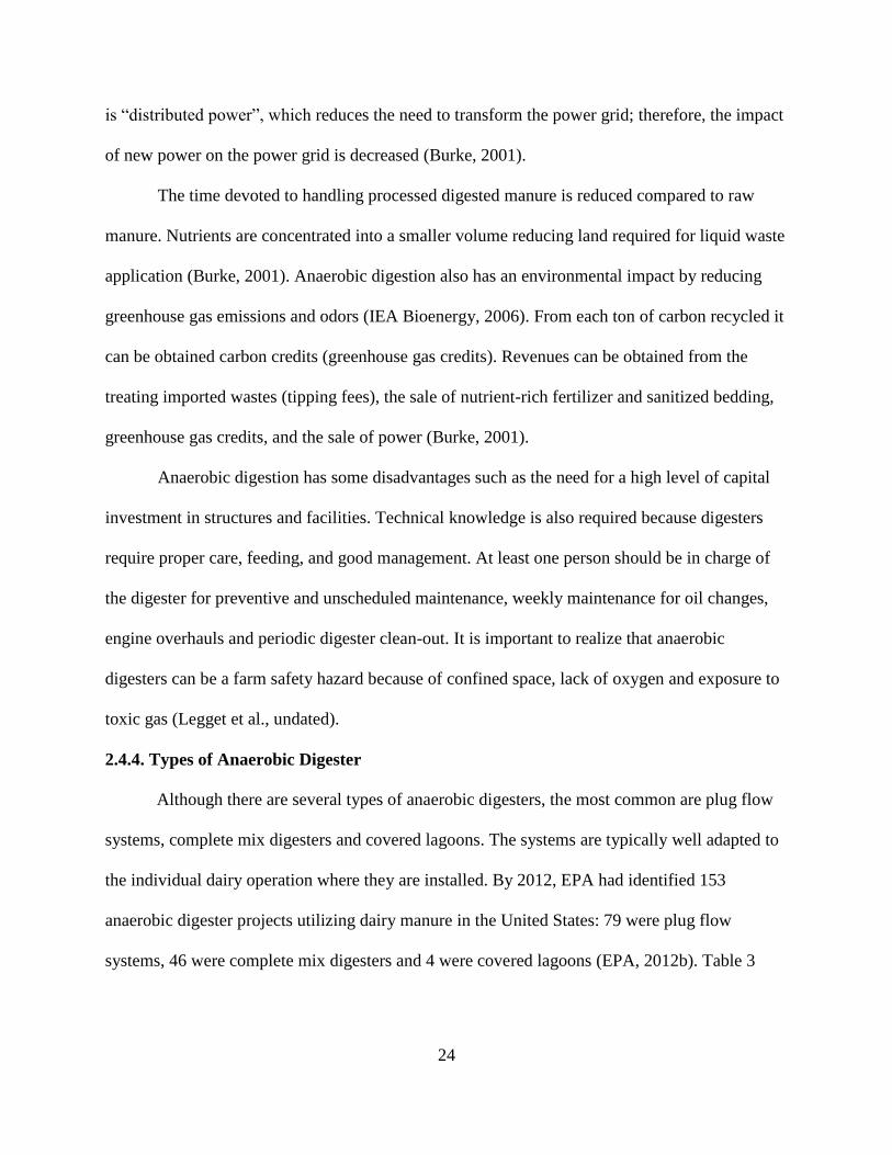
24
is “distributed power”, which reduces the need to transform the power grid; therefore, the impact
of new power on the power grid is decreased (Burke, 2001).
The time devoted to handling processed digested manure is reduced compared to raw
manure. Nutrients are concentrated into a smaller volume reducing land required for liquid waste
application (Burke, 2001). Anaerobic digestion also has an environmental impact by reducing
greenhouse gas emissions and odors (IEA Bioenergy, 2006). From each ton of carbon recycled it
can be obtained carbon credits (greenhouse gas credits). Revenues can be obtained from the
treating imported wastes (tipping fees), the sale of nutrient-rich fertilizer and sanitized bedding,
greenhouse gas credits, and the sale of power (Burke, 2001).
Anaerobic digestion has some disadvantages such as the need for a high level of capital
investment in structures and facilities. Technical knowledge is also required because digesters
require proper care, feeding, and good management. At least one person should be in charge of
the digester for preventive and unscheduled maintenance, weekly maintenance for oil changes,
engine overhauls and periodic digester clean-out. It is important to realize that anaerobic
digesters can be a farm safety hazard because of confined space, lack of oxygen and exposure to
toxic gas (Legget et al., undated).
2.4.4. Types of Anaerobic Digester
Although there are several types of anaerobic digesters, the most common are plug flow
systems, complete mix digesters and covered lagoons. The systems are typically well adapted to
the individual dairy operation where they are installed. By 2012, EPA had identified 153
anaerobic digester projects utilizing dairy manure in the United States: 79 were plug flow
systems, 46 were complete mix digesters and 4 were covered lagoons (EPA, 2012b). Table 3

25
shows a summary of characteristics of digester technologies; Table 4 shows a summary of
process attributes and Table 5 shows an expected percentage of volatile solids conversion to gas.
Table 3. Summary of Characteristics of Digester Technologies (EPA, 2004)
Characteristics Covered Lagoon Complete Mix
Digester
Plug Flow
Digester
Fixed Film
Digestion vessel Deep lagoon
Round/Square
In/Above-
ground tank
Rectangular In-
ground tank
Above ground
tank
Level of
technology Low Medium Low Medium
Supplemental heat No Yes Yes No
Total Solids 0.5-3% 3-10% 11-13% 3%
Solids
characteristics Fine Coarse Coarse Very fine
HRT* (days) 40-60 15+ 15+ 2-3
Farm type Dairy, Hog Dairy, Hog Dairy only Dairy, Hog
Optimum location Temperature and
warm climates All Climates All Climates
Temperature and
warm climates
*Hydraulic Retention Time (HRT) is the average number of days a volume of manure remains in
the digester
Table 4. Summary of process attributes (Burke, 2001)
Attribute Complete
mix-
mesophilic
Complete mix-
thermo
Plug Flow
Mesophilic
Covered
Lagoon
Not limited by solids
concentration
X X
Not limited by foreign material X X
Digest entire dairy waste stream X X
Sand and floating solids
processing
X X
Best at odor control X
Treat additional substrate X X
Stability X X
Simplicity X X
Flexibility
Net energy production X

26
Table 5. Expected percentage VS conversion to gas (Burke, 2001)
Process Load Conversion to gas
Entire Waste Stream
Completely mixed mesophilic High 35 to 45%
Completely mixed thermophilic High 45 to 55%
Partial Waste Stream
Plug mesophilic High 35 to 45%
Covered Lagoon Low 35 to 45%
2.4.4.1. Plug Flow Digester
A plug flow digester is a long rectangular concrete tank with an air-tight cover where
manure flows in one end and out the other with no axial agitation (Betts and Ling, 2009). Some
internal mixing does occur because it is filled daily with biomass (Pennsylvania State University,
2009). Theoretically, as one plug of manure is added to the digester, one plug will leave the
digester. A fraction of methanogens is displaced with the effluent, therefore part of the waste
must be converted to new methanogens because they are not conserved (Burke, 2001).
This type of digester is best suited for thicker manure or waste containing a higher
percentage of solid material (Pennsylvania State University, 2009). They are subject to
stratification, but it can be partially avoided by maintaining a relatively high solids concentration
in the digester (Burke, 2001). The digester is ideal for scraped and partially washed manure
operations (Wilkie, 2005).
2.4.4.2. Complete-mix Digester
The complete mix digester (also referred to as a “continually stirred tank reactor”) heats
and mixes the manure in a cylindrical tank for more efficient biogas conversion. Manure is
mixed by a motor-driven impeller, pump, or other types of devices. The manure is usually heated
in order to maintain a mesophilic or thermophilic environment (Betts and Ling, 2009). Usually,

27
when co-digestion is to be used, a complete mix system is desired, especially when the
characteristics of the added waste are different than manure (Totzke, 2009).
Scraped or flushed systems that are used to clean barns with water generate slurry
manure. Slurry manure contain between three to ten percent of total solids, which works best in
complete mix digesters system (Betts and Ling, 2009). Burke (2001) recommended not using
manure diluted with parlor or flush water with the thermophilic digestion of dairy because
necessary energy will meet the heat requirements.
2.4.4.3. Covered Lagoon
Covered lagoon digesters are best suited for extremely dilute manures stored in an
anaerobic lagoon. It is essentially a pond with a cover that treats liquid manure consisting of less
than 2% solids (Nelson and Lamb 2002). The reaction rate is affected by seasonal temperature
variations (Burke, 2001). Odor may not be entirely removed due to incomplete digestion. They
are more appropriate for flush manure collection systems with total solids of 0.5 to 3 percent
(Betts and Ling, 2009).
These systems have long retention times, between 35 and 60 days, and are generally not
heated. Anaerobic lagoons in climates with low temperatures are the most inexpensive type of
digester (Nelson and Lamb 2002). Thus, they produce more gas in warmer climates but are also
used in northern climates to also reduce odors (Pennsylvania State University, 2009). Increasing
gas yield is accomplished by mixing or heating a lagoon digester, which increases costs.
Periodically, covered lagoons must be cleaned at considerable cost (Burke, 2001).
2.4.5. Dairy Manure Digester
Extensive types of manure pretreatment and treatment options are available. Typical
pretreatment involves screening and gravity separation of the solids. But it is recommended not

28
to use pretreatment processes before anaerobic digestion because they produce odor, are
expensive and impact potential energy generation. However, excess of sands, silts, and fibers
should be removed as part of the anaerobic digestion process. Anaerobic treatment is the most
effective on minimizing odors, producing fertilizer and/or bedding, producing energy and it also
has the lowest operation and maintenance cost (Burke, 2001).
Figure 3 shows the manure characteristics and handling systems that are applicable for
particular types of biogas production systems. Table 6 can help in matching an anaerobic
digester with a facility. The warm and cold climate, described in Table 6, refers to the moderate
to warm region below the 40th parallel and the cold region is above the 40th parallel.
Figure 3. Appropriate manure characteristics and handling systems for specific types of biogas
production systems (EPA-AgSTAR, 2004).

29
Table 6. Matching a Digester to a Dairy Facility (EPA-AgSTAR, 2004)
Climate Collection System Estimated Min.
Ratio of
Water: Manure
%TS Digester Type
Moderate
to warm
Flush 10:1 <3% Covered lagoon
Scrape and parlor
wash water 4:1 – 1.1:1 3% - 11% Complete mix
Scrape manure only N/A >11% Plug flow
Cold
Flush 10:1 <3% Limited possibility for
covered lagoon
Scrape and Parlor
wash water 4:1 – 1.1:1 3% - 8% Complete mix
Scrape manure only N/A >11% Plug flow
Kirk and Faivor (2011) recommend understanding how site-specific conditions influence
the solids characteristics and the biogas potential of the manure. The TS concentration of manure
is a key in selection of an appropriate anaerobic digester and it can vary in several ways
depending on the type of dairy housing facility and use of bedding and manure collection system.
A typical lactating dairy cow can support the production of 1.33 cubic meters (47.1 cubic
feet) of biogas per day (Betts and Ling, 2009). Assuming that the biogas contains 65 percent
methane, this would mean 1.33 cubic meters (47.1 cubic feet) of biogas per day or 0.62 kg (1.37
lb) of methane per cow per day (Table 7).

30
Table 7. Characteristics of lactating dairy cow manure and biogas potential (ASABE, 2005)
Component Units Per cow
Weight Kg/day (lb/day) 68. 04 (150.00)
Volume m3/day (ft
3/day) 0.07 (2.40)
Moisture % 87.00
Total solids Kg/day (lb/day) 9.07 (20.00)
Total volatile solids Kg/day (lb/day) 7.71 (17.00)
Chemical Oxygen Demand Kg/day (lb/day) 8.16 (18.00)
Biological Oxygen Demand Kg/day (lb/day) 1.32 (2.90)
Nitrogen Kg/day (lb/day) 0.45 (0.99)
Phosphorous Kg/day (lb/day) 0.08 (0.17)
Potassium Kg/day (lb/day) 0.1 (0.23)
Biogas production[a]
m3/day (ft
3/day) 1.33 (47.10)
Methane production[b]
m3/day (ft
3/day) 0.87 (30.60)
Methane (CH4)[b] Kg/day (lb/day) 0.62 (1.37)
Btu[c] Kg/day (lb/day) 14.02 (30.90)
kWh[d] 1055 KJ/day (1000 Btu/day) 2.00
Annual kWh per cow Per day 744.00
[a] 90% of the manure collected; 30% conversion rate of COD of methane; 0.18 m3 (6.3 ft
3)
CH4 per lb COD; 65% CH4 in biogas (NRCS)
[b] Biogas with 65% CH4 weighing 0.717 kg/m3 (NRCS).
[c] Represents an average biogas with 65% CH4, where CH4 has a heating value of
35518.4kJ/m3 (1010 Btu/ft
3) CH4 (EPA, 2005).
[d] 66.6 kWh per 28.3m3(1000 ft
3) CH4; assuming 25% thermal conversion efficiency and 90%
run-time (EPA, 2005).
2.4.5.1. Capital cost
The cost of a dairy waste management system involves: housing, collection, pre-
processing, anaerobic digestion, energy production, liquid and handling irrigation, and solids
disposal. Housing determines the amount of manure collected. Manure can be collected
manually, or by automatic scraper, vacuum truck, or flush. Pre-processing (prior to digestion)
and post-digestion (concentration of solids after digestion) can be realized by screening and or
sedimentation. After digestion, energy is produced with an engine generator or turbine with heat

31
recovery. It is also important to know the quantity of digestate produced, to know the storage
size and disposal of liquid waste (Burke, 2001).
EPA-AgSTAR (2010b) analyzed AD system capital cost based on quotes for systems
designed only for manure in 2003–2009. Data was collected from 40 dairy farms; from which 13
were complete mix digesters systems, 19 plug flow digesters, and 8 covered lagoons. The capital
cost for each system includes the cost of the digester, the engine-generator set, engineering
design, and installation. In order to analyze costs evenly, they omitted costs of post-digestion
solids separation, hydrogen sulfide reduction systems, and utility charges including line upgrades
and interconnection equipment costs and fees (EPA-AgSTAR, 2010b) Figure 4 shows while the
smallest farm did have the highest cost per cow for the digester ($1,600), the largest farm did not
have the lowest cost per cow ($750). Farms with the second and third smallest number of cows
had relatively low costs per cow ($700).
Figure 4. Capital cost per dairy cow for complete mix, plug flow, and covered lagoon AD
systems (EPA-AgSTAR, 2010b).

32
The feasibility of setting up an anaerobic digester on a dairy production system will
depend on how the managers use the byproducts (biogas and digestate). The average cost of
additional digester equipment include: 1) post-digestion solids separators, 6.4% of total capital
costs (range from: 1.5-12%), 2) biogas treatment system, 3.1% of total capital costs (range: 0.3-
6.0%) and 3) estimated utility charges, 5.3% (range: 1.7-13.5%). The engine and generator costs
usually account for 40% of project costs (EPA-AgSTAR, 2010b).
In the case of small-scale digesters, U.S. EPA does not recommend biogas recovery
systems for livestock farms with less than 500 cows. Moser (2011) reported that 200-400 cows
were needed for an economically viable digester system. In 2010 the majority (74%) of U.S.
dairy farms had less than 100 cows and in 2011, 88% had less than 200 cows, making anaerobic
digestion not feasible to most of U.S. dairy farms (U.S. Census Bureau, 2012).
Revenue from electricity sales has been profitable for large-scale operations (Nelson and
Lamb, 2002), but small-scale digesters are not often profitable due to their dependence on the
electricity price and the high cost of infrastructure needed to sell electricity back to the grid
(Lazarus and Rudstrom, 2007; Ghafoori and Flynn, 2007).
Electrical generation from biogas was not economically viable but the use of biogas to
accomplish the heating requirements on-farm was found to be economically feasible in small-
scale dairy farms (Bishop and Shumway, 2009). However, Millen (2008) reported on two small
dairy farms (130 and 70 cows) in Ontario that were producing electricity and were profitable.
The farmers credited their success to receiving additional waste (130 cow farm only), having a
buyer for their electricity, and substantial time dedicated to the project development stage.
Several studies have found that direct use of biogas can be profitable on smaller farms
when the on-farm heating requirements were high enough to regularly utilize all the produced

33
biogas (Bishop and Shumway, 2009). Another motivation for farmers to install an anaerobic
digester is the reduction of odor and improvement of air and water quality. A survey of 64
producers across the United States and 10 in California found that both were the main motivation
for digester installation (EPA-AgSTAR, 2007).
Possibly the biggest economic challenge for small-scale digestion systems is the
uncertainty of traditional (e.g. electricity) and non-market factors (e.g. bedding reuse). Stokes et
al. (2008) emphasized the lack of quantifiable data on non-market benefits as a major obstacle to
widespread anaerobic digestion implementation. Another challenge is the cooperation of the
local electrical utility. In many cases this has discouraged dairies from installing digesters that
had been planned (Lazarus, 2008).
The Minnesota Project, a group funded by EPA-AgSTAR, is searching for solutions for
small- and mid-sized dairies. In 2005 they started a feasibility study on the use of the anaerobic
digestion technology by scaling it down and still providing financial incentives for farmers to use
it. The Minnesota Project evaluated six anaerobic digestion systems designed for confinement
dairies between 100 and 300 cows. They concluded that the digester costs, which were between
$105,000 and $230,000, were still too high (Goodrich, 2005).
The Minnesota Project prepared a case study based on the Jer-Lindy confinement dairy
farm in central Minnesota with 97 ha (240 acres) and 160 milking cows producing about 11,356
L (3,000 gallons) per day of manure based on built a small-scale digester with an up-flow tank
system with a 124,918 L (33,000 gallon) holding capacity and five-day HRT. The total a cost of
the system was $460,000 (Table 8) (Lazarus, 2009). In operation several technical and
maintenance issues caused problems: engine failure, computer control system problems and
issues with manure handling (Lazarus, 2009).

34
Table 8. Investment required for similar or any dairy operation with 160 milking cows (Lazarus,
2009)
Items Investment
Digester tank, gen-set and set up $ 267,000
Fan separator $ 36,000
Building costs and concrete $ 33,000
Utility hook up $ 12,000
Flare and boiler $ 13,000
Specific items that vary from operation to operation
Tank insulation $ 32,000
Labor $ 15,000
Additional plumbing and electrical work $ 20,000
Pump and agitator $ 22,000
Excavation $ 10,000
Total digester investment $460,000
The economic analysis evaluated the added value by the generator and the projected costs
of owning and operating it. The analysis assumed that the system would produce 430 kWh of
electricity per day in which 95 kWh was used to run the pumps, digester and fan separation
equipment and 335 kWh per day to replace electricity purchases or to sell back to the grid (Table
9). The manure solids from the separator replaced the sand bedding that normally costs around
$1,000 per month (Table 9) (Lazarus, 2009).
Solids breakdown in the digester was assumed to reduce manure hauling and agitation
costs by $2,400 per year. The most liquid fraction of the digestate could be applied at higher
rates on less areas and possibly reduce the pumping cost (Table 9). The sale of carbon credits due
to the breakdown of methane in the anaerobic digestion process (Table 9) was considered as an
additional source of income (Lazarus, 2009).
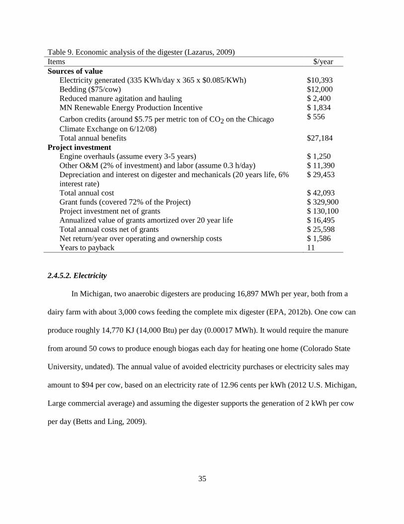
35
Table 9. Economic analysis of the digester (Lazarus, 2009)
Items $/year
Sources of value
Electricity generated (335 KWh/day x 365 x $0.085/KWh) $10,393
Bedding ($75/cow) $12,000
Reduced manure agitation and hauling $ 2,400
MN Renewable Energy Production Incentive $ 1,834
Carbon credits (around $5.75 per metric ton of CO2 on the Chicago
Climate Exchange on 6/12/08)
$ 556
Total annual benefits $27,184
Project investment
Engine overhauls (assume every 3-5 years) $ 1,250
Other O&M (2% of investment) and labor (assume 0.3 h/day) $ 11,390
Depreciation and interest on digester and mechanicals (20 years life, 6%
interest rate)
$ 29,453
Total annual cost $ 42,093
Grant funds (covered 72% of the Project) $ 329,900
Project investment net of grants $ 130,100
Annualized value of grants amortized over 20 year life $ 16,495
Total annual costs net of grants $ 25,598
Net return/year over operating and ownership costs $ 1,586
Years to payback 11
2.4.5.2. Electricity
In Michigan, two anaerobic digesters are producing 16,897 MWh per year, both from a
dairy farm with about 3,000 cows feeding the complete mix digester (EPA, 2012b). One cow can
produce roughly 14,770 KJ (14,000 Btu) per day (0.00017 MWh). It would require the manure
from around 50 cows to produce enough biogas each day for heating one home (Colorado State
University, undated). The annual value of avoided electricity purchases or electricity sales may
amount to $94 per cow, based on an electricity rate of 12.96 cents per kWh (2012 U.S. Michigan,
Large commercial average) and assuming the digester supports the generation of 2 kWh per cow
per day (Betts and Ling, 2009).

36
Various arrangements have been used to capture the value of electricity generated by the
combustion of biogas from anaerobic digestion of manure. EPA (2004) showed the arrangement
for selling on-farm generated electricity:
Biogas sales: The electricity produced is owned by the utility which operates the on-farm
generator. The dairy digester operation sells biogas to the utility and purchases all
electricity needed for dairy operations at retail rates.
All electricity sold: The dairy digester operation sells all its biogas-generated electricity
to a utility (usually at the utilities avoided cost rate) and purchases all the electricity
needed for dairy operations from the utility at retail rates.
Surplus electricity sales: The dairy digester operation generates the electricity needed for
dairy operations on-farm, and excess of electricity produced is sold to the utility (usually
at the utilities avoided cost rate). If the dairy requires any excess of electricity, this will
be purchased from the utility at retail rates.
Net metering: The dairy farm will purchase only the net difference between the quantity
of electricity consumed and the quantity that the dairy digester operation produces.
Binkley (2010) concluded that net metering benefits over the other arrangements for herd
sizes between 500 to 1,450 cows. The farm would not pay charges related to standby or
administration that is based on the capacity of the engine-generator required to produce the
electricity.
2.4.5.3. Biomethane
Biomethane can be upgraded to natural gas containing more than 95% methane.
Biomethane is obtained from gas produced in the digester by removing hydrogen sulfide,
moisture, and carbon dioxide, and when treated correctly it can be used as a substitute of natural

37
gas (Krich et al, 2005). Biogas produced in an anaerobic digester usually contains around 40%
carbon dioxide, however pipeline quality natural gas contains less than 1% carbon dioxide (EPA,
2005), making the conversion from biogas to natural gas costly (Krich et al, 2005). Biomethane
can substitute pipeline quality natural gas which is used for households, commercials or
industries (EPA, 2005). However, few projects have upgraded the biogas to pipeline quality and
provided methane to a nearby commercial natural gas pipeline (Krich et al, 2005).
2.4.5.4. Heat
Almost half of the engine fuel energy can be recuperated with the waste heat which
comes from the engine jacket and exhaust gas. This waste heat can be used for maintaining the
temperature in the digester, heating farm buildings, water, and/or alley floors. Also waste heat
could be used to warm the manure that is entering the digester, reducing the amount of heat used
for changing the manure temperature to the optimum digester temperature (EPA, 2005). Avoided
fuel purchases for heating will depend on the price of fuel and the ability of the operation to
utilize the heat (Betts and Ling, 2009).
2.4.5.5. Digested solids
Using digested solids as cow bedding has advantages and disadvantages. An advantage is
that it may improve cow health (reduced pathogens) and improve milk production (increased
revenue). However, additional equipment and operating costs for separating the digested solids
from the effluent are required. In addition, using digested solids as bedding requires operator
time to avoid potential mastitis problems leading to higher veterinary expenses and lower milk
production and sales (Betts and Ling, 2009).

38
2.4.5.6. Carbon-credits
Methane captured from the anaerobic digestion of dairy manure may meet the
requirements for carbon credits if it is prevented from escaping to the atmosphere. The global
warming potential of methane is equivalent to 25 times that of carbon dioxide (IPCC, 2007).
Reducing one metric ton of methane gas emission has the same impact as reducing 25 metric
tons of carbon dioxide emissions. Based on 2009 national analysis, the use of methane through
anaerobic digesters reduced greenhouse gas emissions by over 1.1 million metric tons of carbon
dioxide in U.S (EPA-AgSTAR, 2010a).
In the United States, there are several trading mechanisms for buying and selling carbon
credits. The transaction could be by private negotiations or trading through formal exchange
mechanisms. It could also be by auction through The World Green Exchange, which provides a
superior price detection system by enabling buyers and sellers to see what the market will
command in real time.
2.4.5.7. Fertilizer
Improved fertilizer value (over raw manure) could allow some sales of effluent, and less
viable weed seeds potentially lower herbicide costs. The minimal odor of the effluent may allow
more flexibility in the timing of land application than for raw manure. This flexibility may afford
economic benefits to the dairy operation.
2.4.5.8. Environment
Using the AD also reduces the water contamination risk, greenhouse gas emission and the
quantity of pathogens. Some firms may be willing to pay the dairy a tipping fee for disposal of
their organic waste. However, this additional substrate will require increased management (e.g.
handling the substrate) and negotiation (Betts and Ling, 2009).

39
2.4.6. Regulations
Odor and water quality complaints accounted for 75% of all complaints related to
livestock facilities registered with the Michigan Department of Agriculture (1,289 observations)
between 1998 and 2007 (Hadrich and Wolf, 2010). The costs of corrective actions on water
quality improvement are significantly higher than odor reductions in dairy farms that incorporate
manure.
In general, small farms are not required to get a permit unless it is proven that pollutants
are discharged to surface water bodies. At that point, farms of any size are required to obtain
permits and follow regulations set forth by the Michigan Department of Environmental Quality
(MDEQ Rector, 2007).
Agriculture impact on greenhouse gases is another important aspect that has been
regulated. Carbon dioxide, nitrous oxide and methane are emitted to and/or removed from the
atmosphere through agricultural activities. The concentrated animal feeding operations (CAFOs)
emit air pollutants that are harmful to public health and damaging the environment. Ammonia
emissions from animal agriculture account for about 50% of the total ammonia emissions into
terrestrial systems (National Research Council, 2003). In 2007, the dairy sector emitted 1,969
million tonnes CO2e (±26 percent) globally of which 1,328 million tonnes was attributed to milk
production (FAO, 2010). Currently, the EPA provides no regulation for air pollution from
CAFOs. Federal laws establish minimum standards for the regulation of any activity that causes
air pollution.

40
2.4.6.1. Federal Regulations related to Anaerobic Digestion
2.4.6.1.1. Air regulations
In general, state permits are required if on-site combustion devices exceed federal
emissions limits. EPA-AgSTAR (2012b) presents federal air permitting requirements for:
Internal combustion engines: should fulfill federal emission standards (40 CFR Part 89)
for non-road engines, which include limits for nitrogen oxides (NOx), hydrocarbons,
carbon monoxide (CO), and particulate matter (PM).
Steam generating devices: Only for the case of devices built after June 19, 1984 and with
a heat capacity over 10.5 million KJ per hour should fulfill federal emission standards
which include limits for PM, sulfur dioxide, and NOx (40 CFR Part 60, Subpart Db or 40
CFR Part 60, Subpart Dc).
Boilers: Only for the case of devices with a heat capacity over 10.5 million KJ per hour
should fulfill National Emission Standards for Hazardous Air Pollutants (40 CFR 63
Subpart DDDD), which include limits for arsenic, cadmium, chromium, lead,
magnesium, mercury, and nickel.
Additionally the Clean Air Act of 2012 requires EPA to set National Ambient Air Quality
Standards (40 CFR part 50) for contaminants harmful to public health and the environment.
Therefore EPA's National Ambient Air Quality Standards (NAASQS) states the limits of
combustion devices emissions such as ozone, PM, CO, NOx and sulfur dioxide.

41
2.4.6.1.2. Solid Waste regulations
Permits for manure solid waste are not required by the federal laws, but in some states the
mixing or use of other types of substrates may denominate the anaerobic digester as a waste
management facility (EPA-AgSTAR, 2012b).
2.4.6.1.3. Water regulations
The discharges by CAFOs are regulated by The Clean Water Act which requires the dairy
facilities a National Pollutant Discharge Elimination System (NPDES) permit. Part of the
discharges to the U.S waters includes improper land application of manure (EPA-AgSTAR,
2012b). For large CAFOs (more than 700 mature dairy cows), additionally to the NPDES permit
a Nutrient Management Plans (NMPs) should be developed and maintained to guarantee correct
land application of manure. If smaller farms discharge to water bodies through a manufactured
device or through direct contact of the animals, they will also be required to have a NPDES
permit and NMPs (EPA-AgSTAR, 2012b).
2.4.6.2. Michigan permitting requirements related to Anaerobic Digestion
Individual states have regulations on how farms operate anaerobic digesters. The
Michigan Department of Environmental Quality presents air and water quality and solid waste
regulations.
2.4.6.2.1. Air permits
Anaerobic digesters require an air permit if combustion is occurring onsite and produces
more than 0.45 kilogram (1 pound) of sulfur dioxide in an hour or has a heat input capacity
greater than 10.5 million KJ per hour, with no difference if organics are included (MDEQ
Rector, 2007).

42
2.4.6.2.2. Solid waste permits
If the anaerobic digester has only manure as biomass, a solid waste permit would not be
required. But if other biomass is added to the digester a permit is needed for composting or land
applying the solids (MDEQ Rector, 2007). There are some substrates that do not require a permit
if the digester receives less than 20% of the substrate, such as food processing waste, syrup from
ethanol production, and grease trap wastes that do not include seepage and fish wastes
(Department of Natural Resources and Environment, 2009).
2.4.6.2.3. Water permits
If the anaerobic digester is operated with only manure a water permit is not required. But
if other types of biomass are added to the anaerobic digester a water permit will be needed for
land application. CAFOs with permission must include an anaerobic digester in their nutrient
management plan (NMP) (MDEQ Rector, 2007).
2.5. Systems Modeling and Simulation
Computer models allow the analyst to predict the effects of changes in complex systems
(Maria, 1997). Models can help to access the benefits, tradeoffs, costs and impacts associated
with management, environment, and other factors (Loucks and Beek, 2005). A model should
accurately represent the system (Maria, 1997). The decision to include or assume information in
the model requires judgment, experience, and knowledge about the issues, the system being
modeled and the decision-making environment (Loucks and Beek, 2005).
Usually, a simulation model is a mathematical representation developed with simulation
software (Maria, 1997). Mathematical models include “known variables” or “parameters” and
“unknown variables” or “decision variables” to be determined. In mathematical terms the model
describes the system being analyzed, and the constraints which are the conditions that the system

43
has to satisfy. Constraints define the system components and their inter-relationships, and the
permissible ranges of values of the decision-variables, either directly or indirectly. Typically,
there exist many more decision-variables than constraints, therefore, if any feasible solution
exists, there may be many solutions that satisfy all the constraints (Loucks and Beek, 2005).
Model parameter values can be uncertain; therefore, the relationship between various
decision variables and assumed known model parameters may be uncertain. This is important
because the output of the model will respond with respect to the parameters and model structures
(Loucks and Beek, 2005).
The model types can be categorized by simulation process, which depends on the
application. The main types of models are those based on simulation period such as discrete and
continuous, and the models based on how they were simulated such as deterministic and
stochastic.
Discrete models advance from event time to event time rather than using a continuously
advancing time (Ündeğer, 2008). Continuous models use time-varying interactions among
variables (Maria, 1997).
Deterministic simulation models use fixed input and output variables (Maria, 1997). The
model does not contain probability. Every run result will be the same, but a single run is enough
to evaluate the result (Ündeğer, 2008). Stochastic simulation models have at least one
probabilistic input or output variable initiated using random numbers (Maria, 1997). Different
runs initiated with different random numbers generate different results. This requires multiple
runs to evaluate the results (Ündeğer, 2008).
No model is perfect. However, modeling and simulation should consider every aspect of
a proposed changes; therefore, operating procedures or methods can be explored without the

44
need of experimenting with the real world systems. Models provide understanding of how a
system operates; therefore, be able to give predictions about how a system will operate under
different scenarios (Ündeğer, 2008). An advantage is a better understanding of interactions
within the variables that make up a complex system. Modeling and simulation determines
answers to “why” questions by recreating the scene and taking a closer look at what has
happened during the run. There can also be answers to “what-if” questions for determining future
improvements and new designs to the system (Ündeğer, 2008).
Simulation modeling also has disadvantages such as special training for model building
and results interpretation, such as determining if an observation is due to system
interrelationships or just arbitrariness. It can also be time consuming and expensive.
Economizing on resources for modeling and analysis may result in a simulation not detailed
enough for the problem and may consume time, effort and money for nothing (Ündeğer, 2008).
There are several models that have been developed for crop modeling, farm economics,
farm environmental and animal modeling.
2.5.1. Crop models
ALFALFA is a dynamic computer simulation model of the growth and development of
alfalfa (University of California, 2010). Crop Environment Resource Synthesis (CERES-Maize)
is a deterministic model that simulates in a field scale corn growth, soil, water, temperature and
soil nitrogen dynamics during one growing season (Ritchie et al., undated). Therefore, CERES-
Maize predicts the duration of growth, the average growth rates, and the economics related to it
(Ritchie et al., 1998).
In order to simulate the carbon and nitrogen biogeochemistry in agro-ecosystems the
Denitrification-Decomposition model (DNDC) was created. The model predicts crop yield, C

45
sequestration, nitrate leaching loss, and emissions of C and N gases in agro-ecosystems. It was
developed by the institute for the Study of Earth, Oceans and Space University of New
Hampshire (University of New Hampshire , 2009). GLYCIM is a dynamic soybean simulation
model with hour time scale. It uses deterministic simulation of organism-level processes
(photosynthesis, transpiration, carbon partitioning, organic growth and development) to predict
growth and yield of a soybean crop depending on climate, soil, and management practices
(Acock and Trent, 1991).
2.5.2. Farm economic models
Some models focus on farm economics such as BIOCOST, which is an EXCEL-based
software program that can be used to estimate the cost of producing bioenergy crops in seven
U.S regions (Walsh and Becker, 1996). FARMSIM is a simulation model used for projecting the
probable economic and nutritional impacts of alternative technologies, farming systems,
livestock management programs, marketing arrangements, crop mixes, risk management
schemes, and environmental remediation programs on a representative crop/livestock farm
(Schaber, undated; Edwards, 2007).
2.5.3. Farm environmental and animal models
Livestock models typically focus on management and economics. Gaseous emissions
submodels are being added to many livestock models. Livestock Analysis Model (LAM)
characterizes cattle and buffalo herds used to produce livestock products: milk, meat, and draft
power. LAM evaluates the impact of changes in production, and present and future methane
emissions from cattle and buffalo populations (EPA, 2010). The Dairy Gas Emissions Model
(DairyGEM) is a process level simulation for estimating ammonia, hydrogen sulfide and

46
greenhouse gas emissions of dairy operations based on climate and farm management (Rotz et
al.,2012).
2.5.4. Whole farm simulation models
Livestock and cropping systems models are often constrained by geographic location or
cropping options. The DairyWise dairy farm model simulates popular feed crops like grazed
grasses or corn (Sendich, 2008). The Dairy Greenhouse Gas Abatement Calculator (DGAS) is
designed for the Australian climate and is not applicable for the Great Lakes Region (The
University of Tasmania, 2013).
Whole farm simulation models such as the Integrated Farm System Model (IFSM) and I-
FARM which integrates crop and animal management components are uncommon (Sendich,
2008). Iowa State University created a whole-farm simulation model called I-FARM, which
predicts economic and ecosystem impacts due to farm operations across the United States. The
model includes several crops and crop rotations with associated tillage, fertilization, planting,
weed control, harvesting, and residue removal. Livestock systems are simulated based on feed
intake, growth rate, grazing or confinement options, and manure management systems (Iowa
State University, 2010). One of the differences between I-FARM and IFSM is that IFSM
integrates anaerobic digestion as a waste management system.
2.5.1. Integrated Farm System Model
The Integrated Farming Systems Model (IFSM) is a whole-farm simulation model that
has been in development since the early 1980’s and was first known as the Dairy Forage System
Model or DAFOSYM. The model operates with a daily time step and includes all major
components of the livestock and crop production system including feed production, storage and
disappearance, animal performance, manure handling, tillage, and planting operations. In order

47
to make the model more comprehensive it was included the simulation of growth, harvest, and
storage of grass, small grain, and soybean, beef production and the option of only crop
production (no animals). An anaerobic digestion sub-model (Rotz et al, 2011b) and
environmental components such as ammonia volatilization, nitrate leaching, phosphorus runoff,
and greenhouse gas emissions were also added (USDA, 2012).
The main difference between IFSM and most farm models is that IFSM simulates all
major farm components on a process level. This allows the components to link the major
biological and physical processes interacting on the farm and is a powerful tool for analyzing the
effects of management and new technologies in the context of the whole-farm system (USDA,
2012). IFSM is designed mainly for temperate regions of the northern United States and southern
Canada.
Belflower (2012) used IFSM to simulate an intensively-managed rotational pasture-based
dairy and a confinement fed dairy in the southeastern part of United States. The study evaluated
management effects on the environment, such as greenhouse gas emissions, carbon footprint, etc.
Rotz et al. (2009) used IFSM to compare the predicted environmental impacts of four different
dairy production systems in Pennsylvania and reported that the use of a grazing system could
reduce erosion of sediment, runoff of soluble P, the volatilization of ammonia, the net emission
of greenhouse gases, and the C footprint.
Rotz et al. (2011a) evaluated environmental and economic impact of manure application
methods in farming systems in Pennsylvania and reported that shallow disk injection was the
most affordable with the lowest environmental influence. Rotz and Hafner (2011b) simulated the
addition of an anaerobic digestion on a dairy farm in New York over 25 years of weather. Farm
records were used to validate the simulations of feed production and use, milk production, biogas

48
production, and electric generation and use. The anaerobic digester decreased net greenhouse gas
emissions and the carbon footprint. The economic analysis showed no direct profits to the
producer.

49
CHAPTER 3: PROCEDURE
A comprehensive analysis was conducted using the Integrated Farm System Model to
describe, evaluate, and compare the economics, resource use and environmental impacts of
representative dairy farms transitioning from conventional confinement to a year round pasture-
based system and the potential for integration of an anaerobic digester in a small confinement
and seasonal pasture dairy.
In order to describe, evaluate and compare a range of farming systems, five
representative dairy farms were compared using the IFSM model. The representative farms do
not describe a specific farm; rather they are designed to reflect common features regarding land
base, machine selection, crop production, number of cows and young stock and other key
components. The five systems include: 1) conventional confinement system with 100 large-
frame Holsteins, 2) conventional confinement system with 100 large-frame Holsteins and an
anaerobic digester, 3) seasonal pasture system with 142 medium-frame Holsteins, 4) seasonal
pasture system with 142 medium-frame Holsteins, an expanded land base for cash crop
production with imported manure and an anaerobic digester and, 5) annual pasture-based system
with 160 small-frame New Zealand Friesian cows. The analysis was conducted over 26 years of
East Lansing, Michigan weather conditions to obtain a comprehensive analysis of system
performance.
Based on farm visits (Appendix A and B) and discussions with dairy farmers considering
the transition from total confinement to an annual pasture-based system, a herd size of 100 cows
is a common tipping point in the decision to continue with total confinement facilities and
expand herd size or maintain herd size and begin the transition to a seasonal or annual pasture-
based system to reduce operating costs. Total confinement systems typically have large-frame
50
Holsteins bred for high milk production. The initial representative farm for analysis was a
milking herd of 100 large-frame Holstein (726 kg mature weight) cows with 80 replacements in
conventional confinement housing and a land base of 111 ha (275 ac, 1.11 ha (2.75 ac) per cow).
This land base balanced feed produced on the farm with small amounts of purchased or sold
forage or grain, and balanced manure nutrient application with crop removal to maintain a near
nutrient balance on the farm.
In a seasonal pasture system cattle are on pasture during summer growing season and
confined during winter. For seasonal pasture systems farmers typically prefer smaller cattle with
traits and genetic potential for milk production between the large-frame and small-frame cows,
such as medium-frame Holsteins. Smaller frame cattle generally consume less feed and produce
less manure than large-frame cattle. Therefore, a seasonal pasture system with 142 medium-
frame Holstein cows (590 kg mature weight) with the same land base as the confinement system
(111 ha) was evaluated as the representative seasonal pasture farm. The land base was held
constant and the cow numbers were increased to maintain the balance between land available for
feed production and the nutrient balance on the farm with only small amounts of forage
purchased or sold.
In an annual pasture-based system, New Zealand Friesian cows (454 kg mature weight)
are the typical cattle (similar to a small-frame Holstein) because of their efficient conversion of
grass to milk. Cattle are supplemented with some dry hay, round bale silage and a small amount
of purchased grain with minimal housing throughout the year. The representative annual pasture-
based system had 160 New Zealand Friesian cows with replacements on the 111 ha (275 acre)
land base. These cow numbers and land base provided a near balance of feed produced and
nutrient use on the farm.
51
Biogas recovery systems on livestock operations can produce renewable energy and
provide additional benefits to the farm. Biogas from anaerobic digestion can heat water and
potentially satisfy other farm energy needs. The digestate can be used as a fertilizer, and bedding
and can be often recovered for reuse. Revenue from electricity generated on-farm can be
obtained through biogas and electricity sale, reduction in purchased electricity use, and in some
cases, net metering (EPA, 2004). Other revenue may be obtained through carbon credits if
methane is captured and prevented from escaping to the atmosphere. The Michigan Department
of Labor and Economic Growth reported that this technology is gaining interest because of new
laws regulating odor, the potential to reduce groundwater contamination, and concerns about
greenhouse gas production (Simpkins, 2005).
Currently, a herd size of 500 cows is considered the break-even point for a typical AD
system for dairy farms (EPA-AgSTAR, 2010b). In this work, this was confirmed by the addition
of an anaerobic digester to the total confinement farm with 100 large-frame Holsteins resulted in
an annual reduction of the net return to management and unpaid factors of more than $14,000 per
year. When an anaerobic digester was added to a 500-cow, total confinement dairy there was an
increase in net return to management and unpaid factors of $9,000 per year. This confirmed that
manure from about 500 cows (about 15,600 t/yr) is needed for a break-even investment on a
typical dairy farm producing energy for on-farm use with recovered bedding.
Seasonal pasture dairies in the Great Lakes region are typically smaller than 500 cows.
Additionally, anaerobic digesters require a steady supply of manure throughout the year for
efficient use. The expansion of many dairy farms is restricted by the lack of land available for
application of manure nutrients. These farms can benefit by exporting manure nutrients for off-
farm use. Cropping systems benefit from the nutrients and other soil quality building factors that

52
livestock manure provides. One alternative for the cost effective integration of an anaerobic
digester on a small, seasonal dairy may be to import manure from nearby dairies, thereby
providing a steady, year round supply of manure in a quantity that is economically feasible.
The economics and performance of the representative 142-cow seasonal dairy was
evaluated when importing 12,882 wet t of dairy manure from nearby dairies (0.75 miles). This
volume of manure, when added to the manure deposited in the barn by the milking herd (2,885
t/yr), provided an annual manure volume similar to that produced on a 500-cow dairy (15,600
t/yr). Additional cash crop land was added to the land base of the seasonal dairy to balance the
additional nutrients with crop removal.
3.1. Representative farm development
Five representative farms were simulated based on information collected from farm visits
(Appendix A and B), literature review and discussions with dairy extension professionals.
Appendix C presents the selected information for each farm. These representative farms were
selected to provide a near balance between the land base and feed produced, and a nutrient
balance between the manure nutrients applied and imported in purchased feed, and the nutrients
used for crop production, exported milk and meat, or otherwise exported from the farm.
3.1.1. Type of dairy farm
The most common housing system on dairies in the Great Lakes Region is the total
confinement system, which typically has cattle inside a free stall barn all year round consuming
rations that are relatively high in concentrates and harvested forages. Large, confined herds
require large structures for housing and feed storage, and material handling equipment and waste
management systems (USDA-NRCS, 2007). Confinement dairies have more control of feed

53
quantity and nutrient concentration during the year, which influences milk production and the
quantity and nutrient concentration in manure (Wattiaux and Karg, 2004).
In an annual pasture-based system cattle are on pasture or open lots throughout the year
consuming grazed forage during the growing season and stored feed throughout the winter.
Pasture-based dairies can reduce feed, labor, equipment, and fuel costs. They provide a lower-
cost option for small farms without the need to expand herd size (USDA-NRCS, 2007).
Mechanical feed harvesting and storage are greatly reduced because the cows harvest the crop
directly from the field much of the year.
Seasonal pasturing has been adopted largely due to the profitability of the dairy industry
in the Great Lakes Region (Nott, 2003). Less purchased feed is required; therefore, fewer
hectares need to be harvested as stored forage. Some producers use seasonal grazing which is a
combination of the two systems and is attractive because it reduces costs by allowing the feeding
of concentrate to improve milk production levels.
3.1.2. Cattle frame
Ninety percent of U.S dairy cows are black and white Holsteins. Holsteins can produce
large volumes of milk, butterfat and protein. When fed high levels of grain the cow can be very
profitable (EPA, 2012a). Cattle frame varies depending on the type of dairy system. Large-frame
Holsteins are typical in conventional confinement systems with a mature body weight of 726 kg
(1,600 lb), bred for high milk production. Cattle in seasonal pasture systems are typically
medium-framed cattle (590 kg mature weight) with traits and genetic potential for milk
production between the large-frame and small-frame cows. Managers of annual pasture-based
systems prefer small-framed New Zealand Friesian cattle (454 kg mature weight) because of
their efficient conversion of grass to milk.

54
3.1.3. Land base
A land base of 111 ha (275 ac) was selected for each of the dairy systems evaluated
(confinement, seasonal pasture and annual pasture) while varying areas for grazing, corn and
alfalfa production. This land base maintained a near balance of feed produced on farm with small
amount of purchased or sold forage or grain, and nutrient balance on the farm with manure
application. The key farm parameters when matching cow numbers with the available land base
were:
Feed production and utilization: indicates how much feed is produced, sold or purchased.
The target was to match feed production with use, with only small amounts of forage and
grain purchased or sold.
Nutrient balance: used to maintain soil fertility with small amount of soil phosphorus and
potassium build-up or depletion.
3.1.4. Milk production
Milk production is a function of genotype, management level, nutrition and
environmental factors. Large-frame Holsteins in confinement typically have greater annual milk
production than small-frame cattle on pasture. The confinement system with 100 large-frame
Holsteins had a target annual (305 days) milk production without fat in the ration of 10,886
kg/cow-yr (24,000 lb/cow-yr). The seasonal pasture system with 142 medium-frame Holstein
cows had a target milk production of 9,071 kg/cow-yr (20,000 lb/cow-yr). The annual pasture-
based system had a target milk production of 7,252 kg/cow-yr (16,000 lb/cow-yr). Potential milk
fat content was 3.5% for the large-frame cows, 3.8% for the medium frame cows and 4.2% for
the small-frame cows (Utsumi, personal communication, 2013). At these production levels
forage quality was the primary constraint to milk production.

55
3.1.5. Type of Manure Treatment
Two types of manure treatment were evaluated: land application of raw manure and
anaerobic digestion. Land application of raw manure means that all manure collected on-farm
was applied to the crop land. When an anaerobic digester was used all the manure collected or
imported was used as biomass for the digester and the digestate from the digester was applied to
crop land.
Five representative farms scenarios were evaluated: 1) conventional confinement system
with 100 large-frame Holstein, 2) conventional confinement system with 100 large-frame
Holstein and AD, 3) seasonal pasture system with 142 medium-frame Holstein, 4) seasonal
pasture system with 142 medium-frame Holstein, imported manure, cash crop and AD and, 5)
annual pasture-based system with 160 small-frame New Zealand Friesian. The different farms
were compared by observing the outputs of farm performance, costs, gas emissions and
footprints (Appendix D). A calculation of the difference between means of each farm was
compared.
IFSM is not currently designed to evaluate an anaerobic digester with imported manure.
Therefore the performance, economics and environmental impact of the seasonal pasture dairy
was approximated by comparing multiple representative farms, one with an anaerobic digester
and a seasonal pasture dairy with imported manure and an expanded land base for cash crop
production and manure use. Because the manure production from a 500-cow dairy is generally
considered to be the threshold for a breakeven investment in an anaerobic digester a 500-cow
confinement dairy with an anaerobic digester was evaluated and found to produce 15,600 t
(17,200 ton) per year of manure. The AD installed on the seasonal dairy was sized to process this
volume of manure (15,600 t) with 2,885 wet t produced by the cattle at the dairy and 12,882 wet

56
t of manure imported from nearby farms. In addition, to evaluate the environmental impact of an
anaerobic digester in the seasonal farm an AD sized to process the amount of manure produced
by 142-cows (2,885 t) was evaluated.
In order to evaluate the integration of a seasonal pasture farm with an anaerobic digester
the differences and percentages obtained between the confinement farm with 500 cows with and
without AD and, between the seasonal farm with 142 cows with and without AD were used
(Table 10 and Table D.1). Information that is not included in Table 10 is the same as the seasonal
dairy farm with 142 medium-frame Holsteins with additional land for cash crop and imported
manure.
Because IFSM does not account for the separate labor and machinery requirements for
imported manure in the seasonal farm with AD, the costs related to importing the additional
manure and the land application of it were calculated, and these costs were added to the farm
production costs (Table C.19). Due to the imported manure the seasonal farm crop land was
increased from 111 ha to 809 ha to achieve a near nutrient balance. Corn acreage was increased
from 75 ha to 374 ha and 374 ha of soybeans were added as a cash crop (Figure 5). Additional
description of farm input parameters are included in Appendix C. Farm performance, economics
and environmental impacts due to the integration of an AD into a seasonal pasture farm were
evaluated by comparing the seasonal dairy farm and the seasonal dairy farm with AD, imported
manure and additional land for cash crop.
The final analysis included the farm performance and economic and environmental
impacts due to the transition from confinement systems to an annual pasture-based system and
the integration of anaerobic digester in a confinement and seasonal pasture system.

57
Farm performance included economics and resource use, annual production costs and net
return to management; crop production costs and total feed costs. Environmental impacts
included nutrients available on farm, used, and lost to the environment; annual emissions of
important gaseous compounds; and environmental footprints of water, nitrogen, energy and
carbon.

58
Figure 5. Development of five representative dairy production systems
Data collected from site visits and literature
review for representative farms
Confinement with
Anaerobic Digester -Large Holstein
-100 cows
-Cows confined year
round
Seasonal Pasture -Medium Holstein
-142 cows
-Cows confined
during winter and
pastured during
summer
Annual Pasture -Small New
Zealand Friesian
-160 cows
-Cows on pasture
all year round
Assumption -Imported manure to
evaluate AD economics
and performance
-Increased crop land to
maintain nutrient
balance
Assumption Type and size of
cows typically used
for confinement
systems in the Great
Lakes Region
Assumption Type and size of
cows typically
used for pasture-
based systems in
the Great Lakes
Seasonal Pasture with
Anaerobic Digester -Medium Holstein
-142 cows
-Cash crop land
-Imported manure
Confinement -Large Holstein
-100 cows
-Cows confined
year round
Assumption Type and size of
cows typically used
in seasonal pasture
system
Assumption -Manure volume
was not
economically
viable for AD

59
Table 10. Estimated values for the seasonal pasture dairy with 142 medium-frame Holsteins, anaerobic digestion, imported manure
and additional land for cash crop production.
Equations used
Nutrients available, used, and lost to the environment
Nitrogen lost by leaching Seasonal 142[a]
w[d]
CC[b]
w Import + (Seasonal 142 w CC w Import * (% Dif.[c]
Seasonal 500[a]
AD-Seasonal 500))
Nitrogen lost by denitrification Seasonal 140 w CC w Import + (Seasonal 140 w CC w Import * (% Dif. Seasonal 500 AD-
Seasonal 500))
Potassium loss through runoff Seasonal 140 w CC w Import + (Seasonal 140 w CC w Import * (% Dif. Seasonal 500 AD-
Seasonal 500))
Soil potassium depletion Seasonal 140 w CC w Import
Crop removal over that
available on farm
Seasonal 140 w CC w Import + (Seasonal 140 w CC w Import * (% Dif. Seasonal 140 AD-
Seasonal 140))
Annual manure production and handling cost
Manure handled Confine 500 AD
Manure applied to corn land Confine 500 AD
Machinery cost Seasonal 140 w CC w Import + (Dif. Confine 500 AD-Confine 500)
Fuel and electric cost Seasonal 140 w CC w Import + (Dif. Confine 500 AD-Confine 500)
Storage cost Seasonal 140 + (Dif. Confine 500 AD-Confine 500)
Labor cost Seasonal 140 w CC w Import + (Dif. Confine 500 AD-Confine 500)
Annual crop production and feeding costs and the net return over those costs
Equipment cost Machinery cost of manure+ Equipment cost of crop-custom cost (Seasonal 140 w CC w Import w
AD)
Facilities cost Seasonal 140 w CC w Import + (Dif. Confine 500 AD-Confine 500)
Energy cost [(Total energy (Mbtu) - Energy Animal housing ventilation and lighting (Mbtu) ) + Excess
electricity (Mbtu)] * 0.028 ($/Mbtu)
Land rental cost Seasonal 140 w CC w Import + (Dif. Confine 500 AD-Confine 500)
Return to management and Costs-Incomes

60
unpaid factors
Annual emissions of important gaseous compounds
Ammonia
Housing facility Seasonal 140 w CC w Import + (Seasonal 140 w CC w Import * (% Dif. Seasonal 140 AD-
Seasonal 140))
Manure storage Seasonal 140 w CC w Import + (Seasonal 140 w CC w Import * (% Dif. Seasonal 140 AD-
Seasonal 140))
Methane
Manure storage Seasonal 140 w CC w Import + (Seasonal 140 w CC w Import * (% Dif. Seasonal 140 AD-
Seasonal 140))
Biogenic Carbon Dioxide
Manure storage Seasonal 140 w CC w Import + (Seasonal 140 w CC w Import * (% Dif. Seasonal 140 AD-
Seasonal 140))
Combustion Carbon Dioxide Seasonal 140 w CC w Import + (Seasonal 140 w CC w Import * (% Dif. Seasonal 140 AD-
Seasonal 140))
Environmental footprints of water, nitrogen, energy and carbon for a dairy farm
Water Use
Production of purchased feed
and inputs
Seasonal 140 w CC w Import
Not allocated to milk
production
Seasonal 140 w CC w Import + (Seasonal 140 w CC w Import * (% Dif. Seasonal 140 AD-
Seasonal 140))
Water footprint with rainfall Seasonal 140 w CC w Import + (Seasonal 140 w CC w Import * (% Dif. Seasonal 140 AD-
Seasonal 140))
Water footprint without rainfall Seasonal 140 w CC w Import + (Seasonal 140 w CC w Import * (% Dif. Seasonal 140 AD-
Seasonal 140))
Reactive Nitrogen Loss
Ammonia emission Seasonal 140 w CC w Import + (Seasonal 140 w CC w Import * (% Dif. Seasonal 140 AD-
Seasonal 140))
Table 10 (cont’d)

61
Nitrate leaching Seasonal 140 w CC w Import + (Seasonal 140 w CC w Import * (% Dif. Seasonal 140 AD-
Seasonal 140))
Nitrous oxide emission Seasonal 140 w CC w Import + (Seasonal 140 w CC w Import * (% Dif. Seasonal 140 AD-
Seasonal 140))
Fuel combustion emissions Seasonal 140 w CC w Import + (Seasonal 140 w CC w Import * (% Dif. Seasonal 500 AD-
Seasonal 500))
Reactive nitrogen footprint Seasonal 140 w CC w Import + (Seasonal 140 w CC w Import * (% Dif. Seasonal 140 AD-
Seasonal 140))
Energy Use
Manure handling Cost for manure handling/ 0.028 (Seasonal 140 w CC w Import /AD)
Production of resource inputs Seasonal 140 w CC w Import + (Seasonal 140 w CC w Import * (% Dif. Seasonal 140 AD-
Seasonal 140))
Not allocated to milk
production
Seasonal 140 w CC w Import + (Seasonal 140 w CC w Import * (% Dif. Seasonal 140 AD-
Seasonal 140))
Energy footprint (Sum Energy Seasonal 140 w CC w Import w AD)/ (lb FPCM Seasonal 140 w CC w Import )
Greenhouse Gas Emissions
(CO2e)
Manure emissions Seasonal 140 w CC w Import + (Seasonal 140 w CC w Import * (% Dif. Seasonal 140 AD-
Seasonal 140))
Emission during feed
production
Seasonal 140 w CC w Import + (Seasonal 140 w CC w Import * (% Dif. Seasonal 140 AD-
Seasonal 140))
Net biogenic carbon dioxide
emission
Seasonal 140 w CC w Import + (Seasonal 140 w CC w Import * (% Dif. Seasonal 140 AD-
Seasonal 140))
Fuel combustion emissions Seasonal 140 w CC w Import + (Seasonal 140 w CC w Import * (% Dif. Seasonal 140 AD-
Seasonal 140))
Production of resource inputs Seasonal 140 w CC w Import + (Seasonal 140 w CC w Import * (% Dif. Seasonal 140 AD-
Seasonal 140))
Not allocated to milk Seasonal 140 w CC w Import + (Seasonal 140 w CC w Import * (% Dif. Seasonal 140 AD-
Table 10 (cont’d)

62
production Seasonal 140))
Carbon footprint without
biogenic CO2
Seasonal 140 w CC w Import + (Seasonal 140 w CC w Import * (% Dif. Seasonal 140 AD-
Seasonal 140))
Carbon footprint w/ biogenic
CO2
Seasonal 140 w CC w Import + (Seasonal 140 w CC w Import * (% Dif. Seasonal 140 AD-
Seasonal 140))
[a] 140/500 = number of cows; [b] CC= cash crop; [c] Dif.= difference; [d] w = with
Table 10 (cont’d)

63
3.2. Herd and crop information of representative farms
The dairy herds included large and medium-frame Holstein cows, small-frame New
Zealand Friesians cows and replacement stock. Dry cows formed 15% of the milking herd. The
land base was selected to provide all forage and grain to a herd of 100 large-frame Holsteins with
only a small amount of forage or grain purchased and sold on an annual basis to balance the feed
produced on the farm. The number of cows in the milking herd was increased to provide a near
nutrient balance on crop removal, available feed and manure produced by the dairy herd (Table
11).
The mature cow body weight was 726 kg (1,600 lb) for the large-framed cows and, 590
kg (1,300 lb) and 454 kg (1,000 lb) for the medium and small-framed Holsteins, respectively.
Potential annual (305 day) milk production without fat in the ration was 10,886 kg/cow (24,000
lb/cow) for the large-frame Holsteins, 9,071 kg/cow (20,000 lb/cow) for the medium-frame
Holsteins and 7,257 kg/cow (16,000 lb/cow) for the small-frame New Zealand Friesian. At these
milk production levels forage quality was the primary constraint. Potential milk fat content was
3.5% for the large-frame cows, 3.8% for the medium frame cows and 4.2% for the small-frame
cows (Utsumi, personal communication, 2013). The herds followed a year-around calving
strategy with a 35% culling rate for the confinement system, 25% for the seasonal pasture system
and 30% for the annual pasture system as a result of healthier lactating cows, with less stress,
more natural diet and, improved reproductive performance (Utsumi, personal comunication
based on Benbrook, et al., 2010). Labor for milking and animal handling was 5.25 min per cow-
day for the confinement system, based on three times per day milking schedule and, 3.0 min per
cow-day for the seasonal and annual pasture systems, assuming 2 times milking per day and
lower milk production (Utsumi, personal communication, 2013) (Appendix Table C.5).

64
Table 11.Major descriptive parameters of five representative dairy production systems
Unit Confine
Confine
w/ AD
Seasonal
Pasture
Seasonal
Pasture
w/ AD[a]
Annual
Pasture
Livestock
Lactating cows - 85 85 121 121 136
Dry cows - 15 15 21 21 24
Young stock over one
year
- 38 38 54 54 61
Young stock under one
year
- 42 42 60 60 67
Alfalfa
Land area ha (ac) 36.4
(90)
36.4
(90)
10.1
(25)
10.1
(25)
40.5
(100)
Harvest system - Hay and
silage
Hay and
silage
Hay and
silage
Hay and
silage
Hay and
silage
Number of cuttings - 4 4 4 4 4
Avg. yield t DM[b]
/ha
(ton DM/ac)
11.78
(5.26)
11.78
(5.26)
11.62
(5.19)
11.61
(5.18)
11.64
(5.20)
Corn
Land area for
confinement
ha (ac) 74.8
(185)
74.8
(185)
50.6
(125)
374
(925)
0
Harvest system - Grain,
silage
Grain,
silage
Grain,
silage
Grain,
silage
-
Number of cuttings - 1 1 1 1 -
Avg. dry corn yield t DM/ha
(ton DM/ac)
6.45
(2.88)
6.41
(2.86)
5.98
(2.67)
6.18
(2.76)
-
Avg. high moisture
yield
t DM/ha
(ton DM/ac)
6.11
(2.73)
6.09
(2.72)
- - -
Avg. silage yield t DM/ha
(ton DM/ac)
12.74
(5.69)
12.64
(5.64)
12.92
(5.77)
13.79
(6.15)
-
Grass
Land area ha (ac) 0 0 50.6
(125)
50.6
(125)
70.8
(175)
Harvest system - - - Silage Silage Silage
Number of cuttings - - - 1 1 1
Avg. yield t DM/ha
(ton DM/ac)
- - 3.78
(1.69)
4.12
(1.84)
3.83
(1.71)
[a] Seasonal Pasture with AD, cash crop and imported manure
[b] t = metric ton; DM=Dry matter
The feed ration was determined by a linear program embedded in IFSM and it was
selected to provide a relatively high forage-to-grain ratio and a minimum of 5% dry hay in cow

65
rations was fed for all farms. The phosphorous and protein were fed at 100% of National
Research Council (NRC) recommendations. Corn grain, corn silage, dry hay, pasture, grass and
alfalfa chopped and baled silage was produced on the farm. A soybean meal crude protein
supplement, distiller grain and minerals were imported to the farm. A loader and mixer wagon
were used for feeding grain and silage. A bale grinder was used for feeding hay (Appendix Table
C.6).
The animal facilities for confinement and seasonal pasture included a double six parlor
milking center, free stall barn naturally ventilated as cow housing, calf hutches and a dry lot as
heifer housing, and short-term storage of premix feed (Appendix Table C.7). Bedding was
chopped straw providing 1.4 kilograms per cow- day (3 lb/cow-day). The purchased bedding for
the farms with an anaerobic digester was reduced to 0.45 kg per cow-day (1 lb/cow-day) because
0.95 kg/d was recycled from the solid part of the digestate (Appendix Table C.8). The annual
pasture-based system included a double-six parlor milking center, calf hutches and a dry lot as
heifer housing with short-term storage for premix feed. No bedding was provided.
Corn and alfalfa were grown on each farm other than the annual pasture-based farm
where only alfalfa and grass/legume pasture were grown. The pasture was 70% cool-season grass
and 30% legume mix pasture on the pasture-based farms. The soil was a medium sandy loam
with total water holding capacity of 19 cm (7.5 in), and soil phosphorus at an optimum level
between of 30 to 50 ppm. Alfalfa had a stand life of 4 years, and grass 10 years. The relative
maturity index of corn was 100 days, with a plant population of 69,189 plants per hectare
(28,000 plants/ac). The P and K balance was achieved with the manure application with a small,
long-term build-up or draw-down. Twenty-eight kilograms per hectare (25 lb/ac) of nitrogen was
applied to the corn at planting time. All manure was applied to land going to corn production.

66
Nitrogen from legumes and manure applied by the grazing animals supplied the nutrients for the
grass pasture. In the annual pasture-based system 80% of manure collected from the milking
center was applied to grass and 20% to alfalfa (Appendix Table C.3).
The confinement, seasonal pasture and annual pasture-based systems had 111 ha
available for crop production. The confinement farm had 36 ha of land in alfalfa and 75 ha for
corn production. The annual pasture-based farm had 40 ha for alfalfa and 79 ha as grazing area.
The seasonal pasture farm had 10 ha for alfalfa, and 51 for corn and 51 ha as grazing area. The
seasonal pasture with additional cash crops and an AD system had additional crop land to
maintain the nutrient balance with the imported manure. The total land area of the seasonal
pasture with cash crop and AD was 809 ha: 374 ha in corn, 374 ha in soybeans, 10 ha in alfalfa,
and 51 ha in pasture (Table 11).
Manure was collected, stored and applied as a semi-solid (12-14% DM), which represents
fresh manure plus bedding. Total manure dry matter was the sum of manure excreted by the
cows plus bedding and feed lost into the manure. Manure characteristics were based ASABE
D384.2 standard (ASABE, 2013a) (Appendix Table C.8). In the confinement and seasonal
pasture-based systems manure was collected with a scraper, stored in a top-loaded, clay-lined
earthen basin and loaded in a slurry spreader tank with a slurry pump. The quantity of manure
handled was dependent on the amount and type of bedding used and the amount of water
contained in the manure. Six months manure storage capacity was provided on the farms with
confinement housing, meaning storage was emptied twice each year in the spring and fall (Table
12). Manure on the annual pasture farm was collected from the milking center with scraper
bucket loading and short-term storage with a few days capacity (daily haul).

67
Manure was imported to the seasonal pasture farm when an AD was used. 12,882 t/yr of
manure was imported and applied to crop land along with 2,885 t/yr produced on the farm.
Additional rented land (809 ha) was used to maintain the whole-farm nutrient balance.
IFSM does not account for the separate labor and machinery requirements for imported
manure (12,882 t/yr). When manure was imported to the farm, additional costs were calculated
and added to the farm ownership and operating costs. Agitation, pumping and trucking manure
from nearby farms to the AD was done on a custom hire basis at $90 per hour assuming custom
hauling with a 22,712 L (6,000 gallons) truck-mounted tank and a 1.6 km hauling distance with a
hauling rate of 52,769 L/h (13,940 gal/h) for 15,812 t of wet manure per year. Custom manure
hauling required 301 hours per year. Machine efficiency and labor hours were calculated based
on Harrigan (2010).
Hauling manure from the AD to the field required two 18,927 L (5,000 gallons) tank
spreaders with 100 kW tractors with an average hauling distance of 1.2 km. The average hauling
rate was 53,942 L/h (14,250 gal/h) and required 148 hours for each tractor and spreader (296 h)
based on Harrigan (2010). Labor for pumping and agitating manure required 42 machine hours
for agitating and pumping, and 8 hours for agitating and clean-up each time the manure storage
was emptied (assumed two times per year) (Appendix Table C.19). Machine efficiency and
labor hours were also calculated based on Harrigan (2010). Repair factors, operating costs,
salvage value and interest rates were calculated based on Hadrich et al. (2010), ASABE standard
D497.7 (2013c) and ASABE standard EP496.3 (2013b) (Appendix Table C.19).
3.3. Tillage and planting information
Tillage and planting operations only occurred on days when soil and weather conditions
were appropriate for field work. A suitable day was when the soil moisture conditions were

68
suitable to support field operations. Depending on the size and type of equipment specified for
each field operation (Table 12), fuel use and labor requirements were determined. A detailed
description can be found in Rotz et al. (2011a).
Tillage and planting operations primarily occurred in the spring and/or fall. For spring
operations, suitable days were determined considering a bare soil (without crop). For summer
and fall operations, suitable days were determined using the soil under or following the growing
crop using the soil moisture after crop production.
Spring operations began with manure application and proceeded through the designated
sequence of tillage operations ending with planting. The number of operations that could occur
simultaneously was two, and the maximum time that tillage and planting operations could be
performed during any given suitable day was 8 hours.
Fall operations were similar to spring operations beginning with manure application or
after some of the crops were harvested. Tillage and planting operations began with alfalfa and
continue with grass and corn. At the end of each simulated year, machine, energy, and labor were
summed.
The sequence of operations of tillage and planting for alfalfa, corn and grass and the
machinery are shown on Table 12. The alfalfa tillage start date was on October 15 using a chisel
plow, followed by a field cultivation beginning April 10 and seeding on April 15. Tillage of corn
ground began on September 10 with spring seed bed tillage beginning on April 10 and corn
planting on May 1, corn operations ended on May 10 with a sprayer. Spring tillage for grass
seeding began on April 15 with field cultivation followed by grass seeding on April 20. Soybean
tillage began on April 10 with field cultivation followed by soybean planting on May 1 and
ended on May 10 with a sprayer (Appendix Table C.14).

69
Table 12. Major machines and structures used for planting and manure storage for five
representative dairy production systems
Machinery or storage type Farm Size Number Price
Tractors and loaders
Transport tractors All farms 35 kW (47 hp) 2-5 $12,000
Round bale loader Confinement 50 kW (67hp) 1 $35,100
Annual pasture 65 kW (87 hp) 1 $54,000
Seasonal 80 kW (108hp) 1 $73,350
Skid-steer loader Annual pasture 15 kW (20hp) 1 $30,600
Confinement and
seasonal
24 kW (33 hp) 1 $39,600
Tillage and planting
Chisel plow All farms 3.7 m (12 ft) 1 $17,100
Seedbed conditioner Confinement and
seasonal
5.8 m (19 ft)
1
$37,800
Annual pasture 4.6 m (15 ft) 1 $30,600
Corn planter Confinement and
seasonal
8 row 1 $31,500
Grain drill Confinement and
seasonal
3.7 m (12 ft)
2.4 m (8 ft)
1
$9,900
Annual pasture 1 $6,750
Sprayer Confinement and
seasonal
15.2 m (50 ft) 1 $9,900
Manure handling and
storage
Slurry tank spreader Confinement and
seasonal
18 t (20 ton) 1 $39,600
Small V-tank spreader Annual pasture 6.0 t (6.6 ton) 1 $24,300
Clay lined storage pit
Confine 1,707 t (1,882 ton) 1 $45,224
Seasonal pasture 1,541 t (1,699 ton) 1 $44,322
Annual pasture 3 day storage slab
and back wall
1 0
Grain harvest and grain crop planting were custom hired, performing the same daily
operations using the determined equipment and operations. Machinery, energy, and labor use
were not considered part of the farm expenses or energy use. The land area tilled and planted for
70
each crop under custom operation was totaled and multiplied by the custom rate to obtain the
total cost. In the annual pasture-based farm forage crop tillage and planting was considered a
custom operation.
Alfalfa and corn harvest procedures were similar for all farms (Appendix Table C.15 to
C.18). Grain harvest was custom-hired for the confinement and pasture-based systems. Corn
silage harvest started on September 1 at a maximum silage moisture content of 68% (wet basis).
High moisture corn harvest started October 1 and dry corn was harvest started on October 21.
Alfalfa was harvest in a four cutting system with the first two cuttings beginning at bud stage on
May 25 and July 1 and cuttings three and four at early flower in mid-August and mid-October.
Alfalfa was mechanically conditioned and raked before harvest. The critical NDF for high
quality storage was 42% for all harvests. Alfalfa was stored as wilted, chopped silage with a
maximum moisture content of 60% on the confinement farms and as round bale silage on the
farms with cattle on pasture from May 25 to October 15. The maximum moisture content for
round bale silage was 68%. Grass for stored silage was harvested at the early head stage with a
maximum moisture content of 60% beginning May 20 when the forage supply exceeded forage
demand.
Corn and alfalfa silage were chopped and stored in bunk silos on the confinement farms
and baled and bagged on the pasture-based farms. Dry hay was baled in round bales and stored
inside a shed. Farms using confinement stored high moisture grain in an upright silo. A large,
portable mixer was used for feed mixing (Table 13) (Appendix Table C.9).
The harvested feed was transported on round bale wagons for hay, dump wagons for
alfalfa and grain crop silage, and grain wagons for grain. All the feed was transported an average

71
of one-half mile for the confinement, seasonal pasture and annual pasture-based systems and
0.75 mile for the seasonal pasture with cash crop system (Appendix Table C.12 and C.13).
Table 13.Major machines and structures used for crop harvest and storage on the five
representative dairy production systems
Machine or
storage type
Confinement Seasonal and Annual pasture
Size Number Price Size Number Price
Mower
conditioner
4.3 m (14 ft) 1 $26,460 2.7 m (9 ft)
3.0 m (10 ft) 1(S)
[a]
1 (A)[b]
$18,900
$20,700
Tandem rake 5.5 m (18 ft) 1 $19,350 5.5 m (18 ft) 1(A) $19,350
Single rake - - - 2.7 m (9 ft) 1(S) $6,300
Round baler Small 1 $20,340 Medium 1 $30,240
Bale wrapping - - - Large 1 $9,720
Forage
harvester
Medium 1 $32,400 Medium 1(S) $32,400
Corn combine 8 row 1 $267,300 8 row 1(S) $267,300
Feed mixer 12 t (13 ton) 1 $63,900 12 t (13 ton) 1 $63,900
Forage blower - 1 $40,050 - 1(S) $40,050
Forage wagons 3.6 t (4 ton) $6,000 $6,000
Hay storage
shed
109 t (120 ton) 1 $25,960 109 t (120 ton) 1 $25,960
Alfalfa bunker
silo
384 t (423 ton) 1 $56,982 82 t (202 ton) 1(S) $32.567
384 t (423 ton) 1(A) $56,982
Corn silage
bunker silo
432 t (476 ton) 1 $61,637 432 t (476 ton) 1(S) $61,637
High moisture
corn stave silo
173 t (191 ton) 1 $38,910 - - -
[a] S = seasonal pasture
[b] A = annual pasture-based
3.4. Economic information
The economic analysis included costs of all major operations on typical farms. The costs
were related to resources grown on and brought onto the farm while income was received for
milk and feed leaving the farm. All monetary returns from milk, feed, and animal sales occurred
in the same year as well as the costs for producing those products. This annual accounting

72
provided a measure of system performance that reflected one year’s use of resources to produce
that year’s production (Rotz et al, 2011a).
The economic information was based on ownership costs determined by amortizing the
initial investment over the life of the system. General economic parameters specify the prices of
energy inputs, the economic life and salvage values of machines and structures, labor wage, land
rental, and the real interest rate (Table 15). Cropping cost parameters include the cost of
fertilizer, seed, and chemicals for producing each crop. Commodity price parameters include the
buying prices of feeds and the selling prices for milk, animals and excess feed. Custom operation
parameters describe the costs associated with hiring a custom operator to carry out specific farm
operations. In this case the hired custom operations were for corn grain harvest and planting,
forage crop tillage and planting and transport of manure from off farm to the AD.
The budgeting process included fixed and variable costs of production. Annual fixed
costs for equipment and structures were a function of their initial cost and economic life which
was 10 years for machinery and 20 years for structures (IRS publication 94b) and a real interest
rate of 6%. Annual fixed costs were summed with annual expenses to obtain a total production
cost. This total cost was subtracted from the total income received for milk, animal, and excess
feed sales to determine a net return to the herd and management (Rotz et al., 2011a). Table 14
presents the major dairy costs and Table 15 presents economic parameters used in all farms,
which were obtained between the years 2011 and 2013 from USDA-NASS, USDA-NRCS, U.S
Energy, Michigan Public Service, Michigan adverse effect wage rate (AEWR), Michigan State
University Extension, Purdue University Extension and Iowa State University (Appendix Table
B.9).

73
Table 14. Major dairy costs ($/cow-year)
Confine Seasonal pasture Annual pasture
Cow housing[a]
$1,400
$1,380 0
Heifer housing[b]
$267 $264 $267
Milking center[c]
$3,120
$2,197 $1,950
Feed facility[d]
$45 $44 $45
Livestock expenses[e]
$551 $359 $418
Total $5,383 $4,244 $2,680
[a] Free stall barn, naturally ventilated
[b] Calf hutches and dry lot
[c] Double six parlor
[d] Short term storage of premix
[e] Includes veterinary and medication, semen and breeding, animal and milking supplies,
insurance of animals, utilities for milking and animal handling, animal hauling and DHIA,
registration.
Table 15. Economic parameters and prices assumed for five representative dairy production
systems
Parameter Value
General rates
Diesel fuel $0.98/L ($3.698/gal)
Electricity $0.13/KWh
Grain drying $ 1.76/pt-t ($1.6/pt-ton DM)
Labor wage $16.13/h
Land rental $126/ha ($50.98/acre)
Property tax 2.5%
Fertilizer prices
N $1.19/kg ($0.54/lb)
P $1.63/kg ($0.74/lb)
K $1.26/kg ($0.57/lb)
Lime $33/t ($30/ton)
Annual seed and chemicals
New forage stand $494/ha ($200/acre)
Established forage stand $17.3/ha ($7/acre)
Corn land $551/ha ($223/acre)
Additional for corn following corn
rotation
$12.4/ha ($5/acre)
Selling prices
Grain crop silage $110/t DM ($100/ton DM)

74
High moisture grain $243/t DM ($220/ton DM)
Corn grain $298/t DM ($270/ton DM)
High quality hay $14/t DM ($13/ton DM)
Milk $0.42/kg ($19/cwt)
Cull cow $1.88/kg ($85.5/cwt)
Bred heifer $300/ animal
Buying prices
Soybean meal 48% $402/ t DM ($365/ ton DM)
Distillers grain $165/t DM ($150/ ton DM)
Corn grain $160/ t DM ($145/ ton DM)
Hay $198/t DM ($180/ ton DM)
Minerals / vitamins $220/t ($200/ ton)
Bedding material $110/t ($100/ ton)
Custom operations
Grain harvest $77.5/ha ($31.4/acre)
Grain crop planting $40.0/ha ($16.22/acre)
Forage crop tillage/planting $138.3/ha ($56.0/acre)
Economic life
Machinery 10 years
Structures 20 years
Machinery salvage value 30%
Real Interest rate 6%
3.5. Pasture growth and management
Part of the forage produced (alfalfa or grass-based) can be fed directly to the animals by
grazing. The grazing area was varied during the spring, summer and fall to reflect the reduction
of land needed when excess forage in the spring exceeded demand, and a small portion of land
lost from production in the fall for grassland renovation. Excess forage in the spring was
harvested as grass silage and stored in plastic-wrapped bales (Table 16). Spring grazing occurred
during the months of April, May, and June; summer grazing in July and August; fall grazing in
September and October. Detailed information about pasture management can be found in Rotz et
al. (2011a).
Table 15 (cont’d)

75
The model provided yield and nutritive content of pastures for the grazed land based on
the GRASIM model. GRASIM predicts pasture production and plant growth for hay and silage
production. For a grass-based pasture, production was simulated in thirty-day intervals between
harvests and makes 60% of the forage for the grazing animals available. The remaining 40% was
considered the initial condition for regrowth.
The required information was investment in fence and watering equipment, and the labor
needed to manage this equipment and the grazing animals. This information was used to
determine the production costs related to pasture. Fence was divided in perimeter and temporary
fence. Perimeter fence was a permanent fence such as high tensile wire. Temporary fence was
movable polywire. Also included in the fencing system are gates and lanes for moving animals
(Table 16) (Appendix Table C.4).
The labor required for pasture management included the time for evaluating pasture and
the animals on that pasture, labor for moving temporary fence and watering equipment, and the
labor required for retrieving animals for milking or moving them to new paddocks (Table 16).
Most of the pasture area was assumed to be clipped once per year. The pasture area
clipped each year was set to the area defined as the summer grazing area. The clipping rate and
fuel consumptions are functions of the size and type of mower used and the tractor used to power
the mower.
The grazing strategy was based on the animal groups placed on pasture and the amount of
time they spent on the pasture. The groups of animals that were on pasture were: older heifers,
dry cows and, lactating cows (Table 16).
The time animals spent on pasture was set as full days during the grazing season (from
April through October), which means between 16 and 18 hours per day (Table 16) for the

76
seasonal pasture farm. The pasture-based farm was set as full days all year, which means
between 18 and 20 hours per day. The animals were maintained outdoors year around even
though pasture growth may not be available during some months. When not on pasture, animals
were housed in the selected facility.
Table 16. Grazing parameters for the seasonal and annual pasture systems
Unit Seasonal Annual
Grazing area
Spring ha (ac) 30.4 (75) 40.5 (100)
Summer ha (ac) 50.6 (125) 70.8 (175)
Fall ha (ac) 40.5 (100) 60.7(150)
Grazing management costs
Investment in perimeter fence $ 3,625 5,075
Investment in temporary fence $ 2,125 2,975
Investment in watering system $ 3,125 4,375
Added annual cost of seed and chemical $/ha ($/ac) 74 (30) 74 (30)
Grazing strategy
Labor for grazing management h/ week 10 10
Types of animals grazed - All cows All cows
Time on pasture h Full days during
grazing
Full days during
grazing
Pasture was allocated along with other available feeds to meet the nutrient needs of each
animal group in the herd. This was done using a partial mixed ration that best complimented the
quantity and nutrient content of the pasture consumed. The pasture consumed was limited by
either what available or the maximum amount of pasture forage that was consumed, which was
the maximum amount of forage that could be included in the animal diet along with the available
supplemental feeds required to maintain the desired production level.
Diets of each animal group were formulated with a linear program set to maximize forage
use in the ration. If there was some excess of pasture forage available on the farm, all the animal
groups that were being grazed could consume that forage in the ration. When forage was

77
supplemented to meet herd needs, pasture was allocated first to grazing heifers and dry cows.
Any remaining pasture was combined with available hay and silage or purchased hay to meet the
roughage needs of the lactating cows. If during one month the pasture ran out before all animals
were fed or during the months pasture was not available, animals were fed using hay and silage.
The nutritive content of pasture varied throughout the grazing season. Crude protein was
set at 26% in the spring, dropped to 23% in the summer, and rebounded to 26% in the fall. Net
energy for lactation started at 1.57 Mcal/kg DM in the spring and slowly decreased to 1.42
Mcal/kg DM in the fall. Neutral detergent fiber started at 52% in the spring, increased to 55% in
the summer, and dropped to 53% in the fall. The rumen degradability of protein was set at 80%
of CP, and the ADIP content was set at 2% of DM. Phosphorus and K contents were a function
of the predominant crop. For grass-based pasture, the assigned P and K contents were 0.35% and
3%, respectively. For alfalfa, the P content was 0.26%, and the K content was 2.5% of DM (Rotz
et al., 2011a).
3.6. Crop nutrient requirements, nutrient availability and loss
An embedded soil model was used to predict moisture and nitrogen available for the
growth and development of each crop. Moisture content was predicted by tracing precipitation
based on 26 years of local weather data, runoff, evapotranspiration, moisture migration, and
drainage through time. Nitrate Leaching and Economic Analysis Package (NLEAP) was the
model used to predict nitrogen cycling in the soil. Each soil layer includes nitrate, ammonia, crop
residue nitrogen, manure organic nitrogen, and other soil organic matter. Nitrogen uptake by the
crop was limited by availability or demand of the crop. Additional information about crop
nutrient requirements can be found in Rotz et al. (2011a).

78
Daily nitrogen losses from the soil due to volatilization, leaching, and denitrification were
also predicted by the model. Volatilization was a function of the amount of ammonia,
temperature, and a volatilization rate. Leaching loss was related to the amount of nitrate and
moisture that drained from the lower layer. Denitrification was a function of denitrification rate,
temperature, and the water-filled pore space in the soil.
The fertilizer application rates included: nitrogen, phosphorous and potassium, and the
percentage of manure applied. The manure application rate was determined by the manure
application divided by the crop land area. Manure nutrients were calculated as dry matter of
manure times the concentration of each nutrient in the dry matter manure. Nitrogen
concentrations of manure were determined after subtracting the losses during collection, storage,
and application.
The nutrient accumulation in the soil and the loss to the environment were predicted by
the whole-farm mass balance. The whole-farm mass balance of nitrogen, phosphorus, potassium,
and carbon was determined as the sum of all nutrient imports in feed, fertilizer, manure
deposition and legume fixation minus the exports in milk, excess feed, animals, manure, and
losses leaving the farm.
The amount of manure applied to each crop was the percentage of the total manure
applied to that crop times the total amount of manure handled annually. The percentage of
manure deposited during grazing was not included in the total manure handled. The amount of
manure applied during grazing was determined by the animal groups and the time they spend on
pasture. For this study the animals were set to be year around on pasture for the annual pasture-
based system and summer grazing for the seasonal pasture system, meaning that about 85% of
the total manure produced was deposited during grazing.

79
3.8. Anaerobic digestion
IFSM predicted the production and use of energy, and the effects that anaerobic digestion
has on manure, nitrogen, phosphorous and economics (Figure 6). The AD manure loading rate
was the amount of manure excreted and collected from barns or transported to the farm from off
farm locations. Biogas is produced through the microbial degradation of the volatile solids in the
manure. Energy production was based on the rate of volatile solids (VS) flow into the digester
from animals. The amount of methane produced was a function of the productivity, which was
set at 0.35 kg CH4/Kg VS (Moller et al, 2007), and a function of the conversion efficiency,
which had typical values close to 35% (Burke, 2001; Rotz et al., 2011a).
Figure 6. Anaerobic Digestion in IFSM
Producing power with biogas was a function of the energy content of methane, which
also depended on biogas leakage (set as a typical value of 15%) (Kirk, personal communication,
2013). IFSM first predicted the amount used to heat water, which was set as 40% of the gas
production, and the remaining was available to generate electricity (Table 17). The amount of
Predicts
Production and use
Changes
Electricity Biogas
Economics Nitrogen and
Phosphorous Manure
AD
Bedding

80
electricity produced each day was limited by either the capacity of the generator, operation time
and the amount of biogas. The efficiency of the engine-generator was set as 35% (Kirk, personal
communication). Any remaining biogas that was not used for either electricity generation or
water heating was burned off in a flare. By burning the biogas the lost carbon converted to
carbon dioxide, which reduced the global warming potential of methane emission.
The initial costs for the anaerobic digester were calculated using a model provided by
Safferman (personal communication, 2013) where the cost of the digester was calculated based
on $7,000/kW and the generator was assumed to be 50% of the cost of the digester. The digester
cost ($7,000/kW) was obtained from a review of like projects around United States and
Michigan State. The initial costs of the digester and generator included: digester structure,
electrical generator, design, construction, planning and, digestate management. The model do not
include modifications required to collect and hold manure prior entering the digester. The costs
may be lower because the electric generation equipment, which is smaller than usual, may be
difficult to find.
The input parameters were: quantity of manure, moisture content, volatile solids, total
solids, volatile solids conversion efficiency and run time efficiency (Table 17). The model
outputs were: initial cost of digester and generator, repair and maintenance cost, electric
generation equipment, gross energy from biomass, net energy from electricity including
efficiency, transportation waste energy, energy for heating influent and to operate AD and, heat
production from generator.
For IFSM only the initial costs of the digester and generator described above, repair and
maintenance costs and, electric generation equipment calculated from the model provided by
Safferman (personal communication, 2013) were used (Table 17).
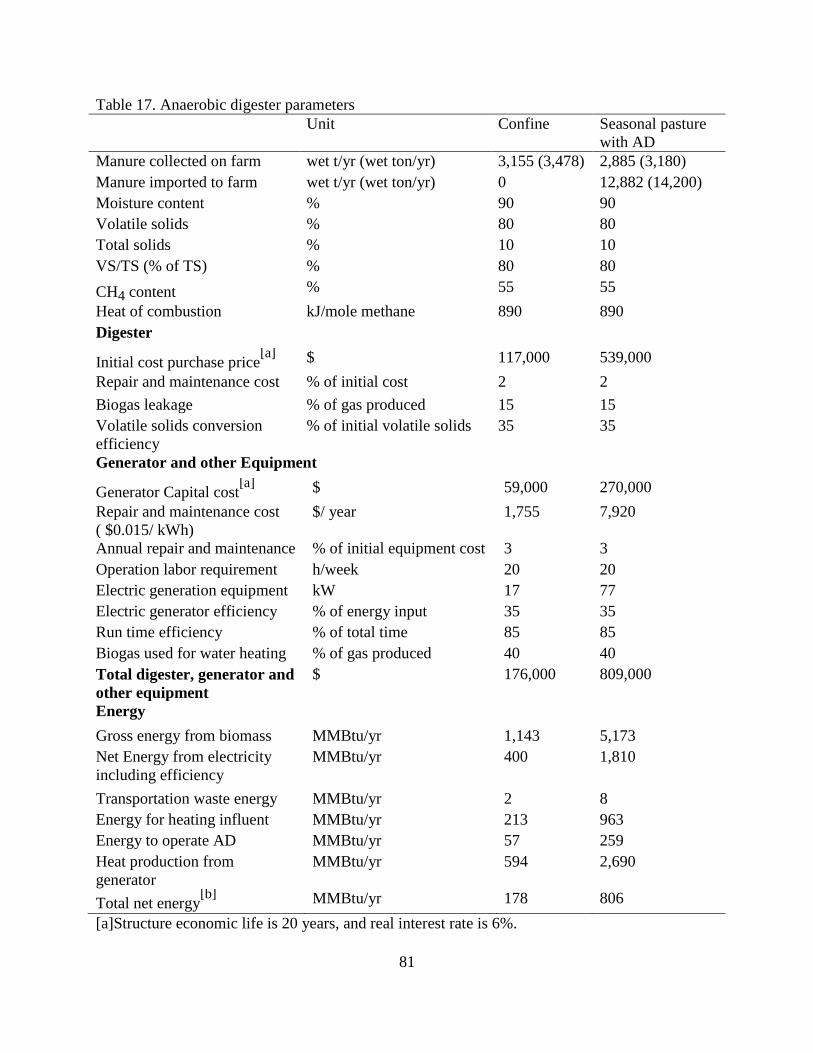
81
Table 17. Anaerobic digester parameters
Unit Confine Seasonal pasture
with AD
Manure collected on farm wet t/yr (wet ton/yr) 3,155 (3,478) 2,885 (3,180)
Manure imported to farm wet t/yr (wet ton/yr) 0 12,882 (14,200)
Moisture content % 90 90
Volatile solids % 80 80
Total solids % 10 10
VS/TS (% of TS) % 80 80
CH4 content % 55 55
Heat of combustion kJ/mole methane 890 890
Digester
Initial cost purchase price[a] $ 117,000 539,000
Repair and maintenance cost % of initial cost 2 2
Biogas leakage % of gas produced 15 15
Volatile solids conversion
efficiency
% of initial volatile solids 35 35
Generator and other Equipment
Generator Capital cost[a] $ 59,000 270,000
Repair and maintenance cost
( $0.015/ kWh)
$/ year 1,755 7,920
Annual repair and maintenance % of initial equipment cost 3 3
Operation labor requirement h/week 20 20
Electric generation equipment kW 17 77
Electric generator efficiency % of energy input 35 35
Run time efficiency % of total time 85 85
Biogas used for water heating % of gas produced 40 40
Total digester, generator and
other equipment
$ 176,000 809,000
Energy
Gross energy from biomass MMBtu/yr 1,143 5,173
Net Energy from electricity
including efficiency
MMBtu/yr 400 1,810
Transportation waste energy MMBtu/yr 2 8
Energy for heating influent MMBtu/yr 213 963
Energy to operate AD MMBtu/yr 57 259
Heat production from
generator
MMBtu/yr 594 2,690
Total net energy[b] MMBtu/yr 178 806
[a]Structure economic life is 20 years, and real interest rate is 6%.

82
[b] Total net energy accounting for all operational needs including transportation, biomass
availability, influent heat, digester heat, digester operation, digester operational time, generator
efficiency, and generator operational time.
The quantity and nutrient content of the manure produced were predicted based on the
feeds consumed and the characteristics of the herd. The digestion process reduced the volatile
solids content in the effluent, reduced the odor and methane produced compared to untreated
manure.
The digestion process also affected the nitrogen fractions in the manure. A portion of the
organic N in the raw manure was decomposed to NH3 and NH4+, also referred as TAN (total
ammoniacal N). IFSM based the amount of TAN in effluent entering long term storage upon data
collected by Gooch et al. (2007), which is modeled as 15% greater than that entering the
digester. This increase in TAN potentially increases the ammonia emissions from the storage and
field applied effluent (Rotz et al., 2011a).
Phosphorous solubility was also increased during the digestion process. The amount of
soluble phosphorus entering long term storage in the digester effluent was increased by 13%
compared to untreated manure (Gooch et al., 2007). The increased solubility affected phosphorus
runoff following field application (Rotz et al., 2011a). Regarding cost, adding an anaerobic
digester to the dairy farm increased the ownership and operating costs and reduced purchased
electricity and bedding cost. When bedding and electricity was produced on the farm, the cost
was reduced in proportion to the reduction in purchased bedding or electricity.
3.9. Environmental impacts
In the environmental section of IFSM, the model does not allow adjustment of
parameters. The environmental impacts modeled by IFSM included volatile, leaching and
denitrification losses of N; volatile loss of hydrogen sulfide; surface runoff and leaching of
Table 17 (cont’d)

83
phosphorous; and greenhouse gas emissions of carbon dioxide, methane, and nitrous oxide. In
addition, other sources of emissions such as ammonia and hydrogen sulfide originating from
manure on the barn floor, the manure storage and field applied manure were included. More
detail about the environmental impacts can be found in Rotz et al. (2011a).
Most of the methane emissions were due to enteric fermentation and long term manure
storage with minor sources being the barn floor, field applied manure, and feces deposited by
grazing animals. Carbon dioxide sources included plant, animal and microbial respiration, both
in soil and stored manure. Nitrous oxide is the strongest of all greenhouse gas emissions
occurring in agricultural production with a global warming potential 298 times that of CO2
(IPCC, 2007). Nitrous oxide sources included nitrification and denitrification processes in the
soil, and these processes also occurred in the crust of slurry manure storage (Rotz et al., 2011a).
The phosphorous cycle is a complex process because it has various chemical forms and
transformations. These processes are modeled in IFSM using relationships from the Erosion-
Productivity Impact Calculator (EPIC) and the Soil and Water Assessment Tool (SWAT) to
better represent surface processes. Surface processes include surface application, runoff, and
transformation along with soil-surface interactions through infiltration and tillage. Erosion
sediment loss is predicted using the Modified Universal Soil Loss Equation (MUSLE).
Total manure nitrogen consists of organic and ammoniacal nitrogen (NH3-N). During
manure handling, ammoniacal nitrogen is transformed and volatilized as ammonia. The primary
source of ammoniacal nitrogen is urine, but a portion of the feces can also transform to an
ammoniacal form during prolonged storage periods. Between 1% and 10% of TAN was lost
when manure was applied through broadcast spreading. When manure was applied to a soil

84
surface, the TAN readily volatilized as ammonia. Therefore, its amount varied through time.
During each time step, ammonia loss occurred to the atmosphere and TAN moved into the soil
through infiltration.
Hydrogen sulfide is mainly created and emitted from decomposing manure under
anaerobic conditions. Main sources include the barn floor and long-term manure storage with
minor losses following field application. Hydrogen sulfide is one of the contributors of manure
odor. It is also a toxic compound when the concentration builds up in a confined space such as
enclosed manure storage.
Environmental footprints are expressed as the environment impacts per unit of product.
In IFSM, four environmental footprints were evaluated: water use, reactive N loss, energy use,
and carbon emission. A footprint was determined by summing the estimates for each of the uses
(removing that allocated to co-products), and dividing by the amount of milk produced.
Functions or factors were used to estimate values for important uses in the production
system. This includes the major uses of water, fossil fuel, and the reactive nitrogen and GHG
emissions that occur during the manufacture of resources used in the production system.
Secondary uses can include the manufacture or production of fuel, electricity, machinery,
fertilizer, pesticides, seed, and plastic used on the farm. Other secondary inputs include any feed
or replacement animals purchased and imported to the production system.
The major water requirement was for the production of feed crops. Other uses include
drinking water for animals, water used for animal cooling, cleaning of the parlor, and holding
areas on dairy farms.
Reactive nitrogen is essential in the growing of crops and feeding of animals. Only
nitrogen in this form can be taken up by crops to form the proteins needed by the animal. The

85
increase in reactive nitrogen in our environment is a concern due to its effect on natural
ecosystems and contributions to other forms of air and water pollution. Primary losses of reactive
nitrogen include ammonia and nitrous oxide emissions to the atmosphere, nitrate leaching to
ground water, and the combustion of fuels.
The energy footprint is defined as the total energy required to produce feed and milk,
except for the solar energy captured by the growing feed crops. This includes all fuel and
electricity directly used in the production system as well as the secondary energy used in the
production of resources used on the farm. One of the major uses of energy on farms is the fuel
used to operate tractors and other equipment for feed production, feeding, and manure handling.
Fuel use was converted to energy units assuming 35.8 MJ/L of fuel. Electricity was another
major use mainly for milking, ventilation, and lighting. Electrical use was converted to energy
units (3.6 MJ/kWh of electricity).
Carbon footprint is the total GHG emission expressed in CO2 equivalent units (CO2e).
The conversion factor for CH4 and N2O are 25 and 298 CO2e/kg, respectively (IPCC, 2001;
EPA, 2007). The carbon footprint was primarily determined as the net emission of the three
GHGs including all sources and sinks of CO2. A carbon balance was enforced, so a portion of
the CO2 assimilated in the feed was in the carbon exported during feed, milk, and animal
productions (Rotz et al., 2011a).

86
CHAPTER 4. RESULTS AND DISCUSSION
The IFSM model was used to analyze the transition from a 100-cow conventional
confinement dairy to an annual pasture-based system. The analysis included economics and
resource use, farm performance and environmental impacts of representative farms. The
representative farms included year-around confinement with conventional large-frame Holstein
cattle; seasonal pasture with winter confinement and summer pasture with medium-frame
Holsteins; an annual pasture-based dairy with New Zealand-style Friesian cattle whereby the
cows were on pasture or open lots throughout the year; and the integration of an anaerobic
digester on a total confinement dairy and a seasonal pasture dairy with imported manure and an
expanded land base for cash crop production and manure application.
The representative dairy systems were compared on a fixed land base (111 ha) with large-
medium- and small-framed cattle, except the seasonal pasture with AD which had a land base of
809 ha. The base farm for comparison included 100 large-frame cows (85 milking, 15 dry cows)
with 80 replacements over 26 years of Lansing, MI weather. Based on the nutrient balance when
producing alfalfa, corn silage and corn grain while importing some concentrate and returning the
manure nutrients to the land for crop production, the nutrient balance with 100 large-frame cattle
with replacements was similar to a seasonal dairy with 142 medium-frame cattle and an annual
pasture-based dairy with 160 small-frame cattle plus replacements.
4.1. Comparison of farm performance and resource use
The transition from conventional confinement to a pasture-based system affected feed
production and the purchase of feed supplements, milk and manure production. Overall, feed
consumption increased 23% with the seasonal pasture and 12% with the annual pasture-based
87
system compared to confinement because grazed forage was added to the cattle diet replacing
high moisture grain and some alfalfa silage (seasonal pasture) and grain silage (annual pasture).
On-farm feed production varied depending on the type of dairy and decreased from confinement
to seasonal to annual pasture-based systems. The seasonal pasture produced 15% less milk per
cow-yr compared to confinement and the annual pasture-based system produce 31% less per
cow-yr. The confinement farms collected more manure than the seasonal and annual pasture-
based farms because the cows stayed inside the barn year-around. Additional discussion and
detail follows.
4.1.1. Milk, feed and manure production
The annual target milk production (305 day) without fat in the ration was 10,886 kg/cow
(24,000 lb/cow) for the large-frame Holsteins, 9,071 kg/cow (20,000 lb/cow) for the medium-
frame Holsteins and 7,257 kg/cow (16,000 lb/cow) for the small-frame New Zealand Friesians.
The annual milk production with the feeds fed was 9,946 kg/cow for the large-frame Holsteins,
8,482 kg/cow for the medium-frame Holsteins and 6,829 kg/cow for the small-frame New
Zealand Friesians (Table 18). Because fat was not fed in the diet, forage quality was the limiting
factor in milk production. Total annual milk production was 845,430 kg for the large-frame
cattle, 1,026,277 kg with the medium-frame cattle and 928,753 kg with the small-frame cattle.
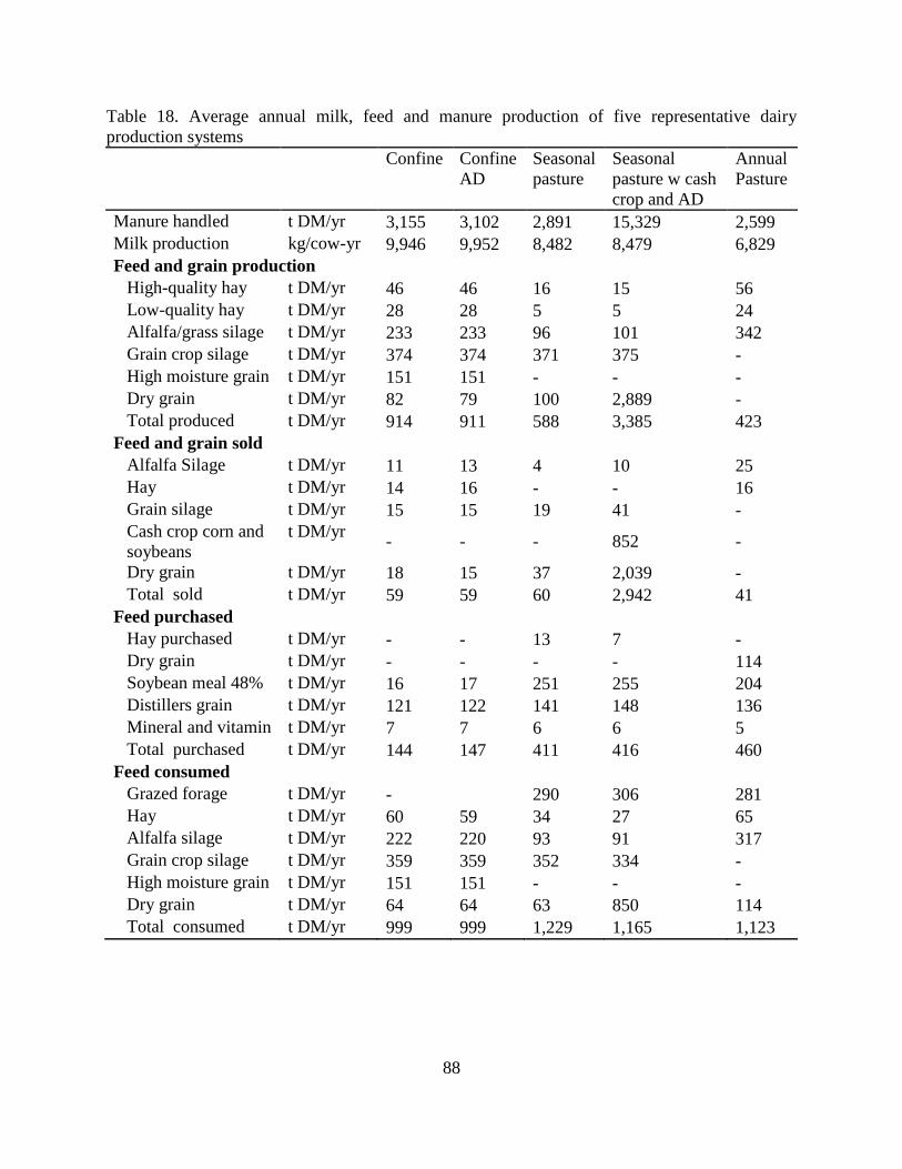
88
Table 18. Average annual milk, feed and manure production of five representative dairy
production systems
Confine Confine
AD
Seasonal
pasture
Seasonal
pasture w cash
crop and AD
Annual
Pasture
Manure handled t DM/yr 3,155 3,102 2,891 15,329 2,599
Milk production kg/cow-yr 9,946 9,952 8,482 8,479 6,829
Feed and grain production
High-quality hay t DM/yr 46 46 16 15 56
Low-quality hay t DM/yr 28 28 5 5 24
Alfalfa/grass silage t DM/yr 233 233 96 101 342
Grain crop silage t DM/yr 374 374 371 375 -
High moisture grain t DM/yr 151 151 - - -
Dry grain t DM/yr 82 79 100 2,889 -
Total produced t DM/yr 914 911 588 3,385 423
Feed and grain sold
Alfalfa Silage t DM/yr 11 13 4 10 25
Hay t DM/yr 14 16 - - 16
Grain silage t DM/yr 15 15 19 41 -
Cash crop corn and
soybeans
t DM/yr - - - 852 -
Dry grain t DM/yr 18 15 37 2,039 -
Total sold t DM/yr 59 59 60 2,942 41
Feed purchased
Hay purchased t DM/yr - - 13 7 -
Dry grain t DM/yr - - - - 114
Soybean meal 48% t DM/yr 16 17 251 255 204
Distillers grain t DM/yr 121 122 141 148 136
Mineral and vitamin t DM/yr 7 7 6 6 5
Total purchased t DM/yr 144 147 411 416 460
Feed consumed
Grazed forage t DM/yr - 290 306 281
Hay t DM/yr 60 59 34 27 65
Alfalfa silage t DM/yr 222 220 93 91 317
Grain crop silage t DM/yr 359 359 352 334 -
High moisture grain t DM/yr 151 151 - - -
Dry grain t DM/yr 64 64 63 850 114
Total consumed t DM/yr 999 999 1,229 1,165 1,123
89
The seasonal pasture produced 1,465 kg/cow-yr less milk and the pasture-based system
produced 3,117 kg/cow-yr less milk than the confinement dairy. Generally, milk production per
cow is lower on pasture-based than confinement systems (Winsten et al, 2000). Reduced milk
production in pasture-based systems is usually because of the additional energy the cow expends
in harvesting its own forage and the difficulty in balancing cow rations (Muller and Holden,
1994). Typically, the diets of grazing cattle are higher in forages and lower in grain and
concentrate. The annual diet in the seasonal pasture system was 24% grazed forage and the
annual pasture was 25% grazed forage (Table 18).
Feed consumption (including grazed forage) increased by 231 t DM/yr with the seasonal
pasture and 124 t DM/yr with the pasture-based system compared to confinement (Table 18). In
the seasonal pasture system there was no high moisture corn fed and 129 t DM/yr of alfalfa
silage and 26 t DM/yr less hay was fed compared to confinement; however, this was replaced by
290 t DM/yr of grazed forage. In the annual pasture no high moisture corn or grain crop silage
was included in the cattle diet but was replaced by 95 t DM/yr of alfalfa silage, 51 t DM/yr of
dry grain and 281 t DM/yr of grazed forage.
Feed production varied with the cropping system. The confinement and pasture-based
dairies produced more high and low quality hay (between 24 and 56 t DM/yr), and more alfalfa
and grass silage (between 233 and 342 t DM/yr). The seasonal pasture dairy produced 16 t
DM/yr of high quality hay and 5 t DM/yr of low quality hay because only 10 ha were allocated
for alfalfa production. The confinement and annual pasture-based systems allocated 36 ha and 40
ha, respectively (Table 18).
The pasture-based system did not produce any grain. Grain crop silage production was
similar for the confinement and seasonal pasture systems (between 371 and 375 t DM/yr)

90
because the confinement dairy had 75 ha for corn production and the seasonal pasture had 51 ha
available. The seasonal pasture with an expanded land for cash crop and AD produced 2,808 t
DM/yr of dry grain more than the confinement farm because of the increased crop land in corn
(374 ha) and soybean (374 ha) ground. Because of the increased crop land the seasonal pasture
with AD produced the greatest quantity of feed sold per year (2,942 t DM/yr) compared to the
confinement (59 t/yr), seasonal pasture (60 t/yr) and the annual pasture-based systems (41 t/yr)
(Table 18).
The confinement dairy purchased 144 t DM/yr of feed compared to 411 t DM/yr for the
seasonal pasture and 460 t DM/yr for the annual pasture system. The reduction was primarily
soybean meal, 188 and 235 t DM/yr compared to the seasonal pasture and annual pasture-based
system, respectively (Table 18). Eighty-six percent of the feed consumed on the confinement
dairy was produced on-farm and 14% was purchased. The seasonal pasture system produced
67% of total feed consumed and 33% was purchased. The annual pasture dairy produced 59% of
the total feed consumed and purchased 41%. The seasonal pasture with expanded land for cash
crop and AD system produced 64% of total feed consumed, 36% was purchased and the
remaining crops were sold.
The confinement dairy collected more manure (3,155 wet t/yr) than the seasonal pasture
(2,891wet t/yr) and annual pasture dairies (2,599 wet t/yr) because the cows were confined in the
barn throughout the year.
4.2. Economics
The evaluation of farm economics accounted for the major costs related to manure
handling and production on-farm and their income from milk and animal sales. Main production
costs analyzed on farm were: equipment, facilities, energy, labor, land rental, custom operations,

91
crop production, feed costs and animal expenses. The analysis relates these costs with the type of
dairy system (confinement, seasonal pasture or annual pasture-based) and the addition of an
anaerobic digester.
Overall, the seasonal pasture with imported manure, expanded land base for cash crop
production and an integrated anaerobic digester had the highest annual cost for manure handling
($146,985/yr), followed by the confinement dairy with AD ($63,077/yr), seasonal pasture
($36,595/yr), confinement ($35,225/yr) and annual pasture ($15,969/yr), respectively. The
seasonal pasture had the highest production cost ($517,738/yr) followed by confinement with
AD ($450,238/yr), confinement ($435,960/yr) and annual pasture ($435,894/yr). The seasonal
pasture with imported manure, cash crop production and AD had the lowest production cost
($183,481/yr) and the highest net return to management and unpaid factors ($420,192/yr)
followed by annual pasture ($88,162/yr), seasonal pasture ($86,133/yr), confinement
($73,594/yr) and, confinement with AD ($62,578/yr). Additional discussion and detail follows.
4.2.1. Manure handling costs
Manure was collected, stored and applied as a semi-solid (12-14% DM). In the
confinement and seasonal pasture systems manure was collected with a scraper, stored in a top-
loaded, clay-lined earthen basin with 6-month storage capacity and loaded in a slurry spreader
tank with a slurry pump. The bedding was chopped straw supplied at 1.4 kilograms per cow- day
(3 lb/cow-day). For the annual pasture system manure was collected only in the milking center
with scraper bucket loading and short-term storage with a few days capacity (daily haul). No
bedding was added on the pasture-based system.
The seasonal pasture with imported manure and an anaerobic digester had the highest
cost for manure handling, followed by confinement with anaerobic digestion, seasonal pasture,

92
confinement, and annual pasture. In the confinement and seasonal pasture systems the annual
costs for manure handling were: machinery, bedding, labor, storage and fuel and electricity cost
(Table 19). The costs for the annual pasture were: machinery, labor and, fuel and electricity
costs. There was no storage and bedding cost because manure was hauled daily and no bedding
was provided.
Table 19. Manure handling costs ($/year) for five representative production systems
Confine
Confine
AD
Seasonal
pasture
Seasonal
pasture w cash
crop and AD
Annual
Pasture
Machinery 16,468 14,097 18,762 25,360 8,562
Fuel and electric 1,947 1,677 1,771 6,836 1,790
Storage 3,943 24,062 3,864 96,246 -
Labor 4,561 20,473 4,114 15,848 5,617
Bedding 8,306 2,768 8,084 2,695 -
Total manure handling 35,225 63,077 36,595 146,985 15,969
The major costs for confinement with AD were storage ($24,062/yr) and labor
($20,473/yr). Storage cost increased 6 times ($20,119/yr) and labor 4 times ($15,912/yr)
compared to confinement without AD. The storage cost increased because of the addition of the
anaerobic digester which included design, construction, installation, generator and digester. The
total capital cost for the digester, generator and other equipment was $141,000/yr. Labor
increased because 20 additional hours per week were required for maintenance of the digester.
The seasonal pasture with imported manure and AD followed a different trend than
confinement and seasonal pasture. Total manure handling cost increased 4 times ($110,390/yr)
compared to the seasonal pasture without AD. Storage cost was $92,382/yr greater than the same
farm without an anaerobic digester and imported manure because of the investment in the
digester and related equipment (Table 19). Machinery costs for hauling manure increased

93
$6,598/yr, fuel and electric cost increased $5,065/yr and labor increased 4 times ($11,734/yr)
compared to the same farm without an anaerobic digester and imported manure. The increase
was from hauling the imported manure from the farm where was produced to the anaerobic
digester and then hauling and land application of the digestate.
4.2.2. Production costs
The seasonal pasture had the highest production cost, followed by confinement with AD,
confinement and annual pasture (Table 20). The seasonal pasture with AD had the lowest
production cost.
Table 20. Total production costs ($/year) for five representative dairy production systems
Confine
Confine
AD
Seasonal
pasture
Seasonal
pasture w cash
crop and AD
Annual
Pasture
Equipment 98,926 98,090 95,937 92,017 51,273
Facilities 84,452 104,581 85,262 177,623 57,599
Energy 21,871 5,348 20,196 13,293 15,998
Labor 73,943 89,828 64,294 81,912 71,418
Custom operation 3,093 3,078 3,295 97,677 2,380
Seed, fertilizer and
chemical 51,111 51,112 38,949 340,373 17,128
Land rental 5,270 5,270 5,270 96,178 5,270
Net purchased feed
and bedding 21,791 17,414 120,973 (799,143) 120,873
Animal purchase and
livestock expense 46,600 46,600 50,978 50,978 66,880
Milk hauling and
marketing fees 23,730 23,744 27,370 27,359 23,348
Property tax 5,173 5,173 5,214 5,214 3,727
Total production costs 435,960 450,238 517,738 183,481 435,894
The major production costs in the confinement and seasonal pasture systems were for
equipment, facilities, labor, seed, fertilizer and chemical and animal purchase and livestock
expenses (Table 20). The seasonal pasture had higher facilities costs and animal purchase and

94
livestock expenses compared to the confinement system because these costs increased with the
number of cows. The confinement system had higher costs for labor, seed, fertilizer and
chemicals because it had more crop land for corn and alfalfa production (111 ha) than the
seasonal pasture (61 ha) due to the shift in land for grazing animals.
The transition from confinement to a seasonal pasture system increased production costs
by 18% ($81,778/yr). The transition from confinement to annual pasture decreased production
costs by $66/yr (Table 20). The increase in production cost in the seasonal pasture system was
because of the increase in purchased feed which was 3.4 times more ($91,515/yr) than the
confinement system. The seasonal dairy purchased 235 t DM/yr of soybean meal and 20 t DM/yr
of distillers grain more than the confinement system (Table 18) because of the decrease corn
production and the change in diet which included 24% of grazed forage.
The annual pasture dairy had production costs similar to the confinement system (Table
20). Although housing, machinery, manure handling and other costs decreased on the annual
pasture dairy, net purchased feed cost increased ($99,082/yr) with the purchase of 204 t DM/yr
more of soybean meal, 136 t DM/yr more distillers grain and 114 t DM/yr of dry grain (Table
18). These energy and protein feeds were needed to approach the target milk production level.
Animal purchase and livestock expenses increased by 44% ($20,280/yr) for the annual
pasture dairy compared to the confinement dairy because of the increase in cow numbers. Most
livestock expenses are related to the number of first lactation animals (Utsumi, personal
communication, 2013), therefore high replacement rates are driven by the need to cull cows with
recurrent health problems. Grazing cows tend to have fewer serious health problems and
improved reproductive performance (Benbrook et al., 2010), therefore, for the annual pasture
system 25% were first lactation animals and for the confinement system 35% were first lactation

95
animals. Even though the annual livestock expenses were less ($418/cow-yr) for the annual
pasture system compared to the confinement system ($551/cow-yr), total livestock expenses
were higher for the annual pasture system because there were more animals on the farm.
Compared to confinement, the annual pasture-based system had the greatest reduction in
the cost of seed, fertilizer and chemical (66%, $33,983/yr), equipment cost (48%, $47,653/yr),
energy cost (27%, $5,873/yr), labor cost (3%, $2,525/yr), property tax (28%, $1,446/yr) and,
custom operation (23%, $713/yr) because there was no grain crop production. There was a
decrease of 32% ($26,853/yr) in facilities cost because the annual pasture-based system did not
have a structure for cow housing (Table 20).
Production costs for the seasonal pasture with AD and additional land for cash cropping
decreased $252,479/yr because of $820,934/yr decrease in net purchased feed and bedding cost
compared to the confinement system. There were 2,942 t DM/yr feed sold compared to 60 t
DM/yr sold by the confinement farm. The return from feed and cash crop sales more than offset
the increased costs of custom hire, seed, fertilizer and chemicals, and land rental (Table 20).
The addition of the anaerobic digester on the seasonal farm with additional land for cash
cropping increased facilities cost by 108% (92,361/yr) and labor cost by 27% ($17,618/yr)
compared to the seasonal pasture without AD. Energy cost decreased by 34% ($6,903/yr)
compared to the seasonal farm without AD and without an expanded land base. Comparing a
seasonal farm with cash crop and imported manure without AD with the representative seasonal
farm with expanded cash crop, imported manure and AD there was a reduction in energy cost by
68% ($28,321/yr). This included a 16% decrease ($1,318/yr) in energy for manure handling for
the reduction in the amount of purchased bedding from 1.4 kg/cow/day (3 lb/cow/day) to 0.4
kg/cow/day (1 lb/cow/day). There was a 33% ($2,346/yr) decrease in energy for milking and

96
milk cooling related to water heating that was partially replaced by gas from the digester. Energy
for animal housing, ventilation and lighting ($1,500/yr) was completely offset the biogas
produced by the AD.
The major reduction of energy costs with the AD was a reduction of 24% ($3,971/yr) in
electricity purchased (production of resource inputs). Additionally, there was 352,783 MBtu/yr
more electricity produced than consumed by the farm, and this was sold. However, the selling
price was the same as the buying price which over-estimated the farm selling price. The revenue
from electricity sold was $9,878/yr.
The confinement system with AD experienced an increase in facilities costs of 24%
($20,129/yr) and labor by 21% ($15,885/yr) due to the anaerobic digester. Bedding costs
decreased 20% ($4,377/yr). Energy cost was reduced by 76% ($16,523/yr).
4.2.3. Income and net return
Income from milk sales was higher in the seasonal pasture system ($520,062/yr) followed
by confinement ($450,900/yr) and the annual pasture ($443,650/yr). The annual milk production
of the farms was 8,482 kg/cow for the seasonal pasture system, 9,946 kg/cow for the
confinement system and 6,829 kg/cow for the annual pasture-based system. Even though the
confinement had higher milk production per cow, the income from milk sales was higher for
seasonal pasture farm because it had more lactating cows than the confinement farm.
Income from animal sales increased 36% ($22,155/yr) with the seasonal pasture system
and 30% ($18,752/yr) with the annual pasture-based system compared to confinement (Table
21). The difference was related to the culling rate; 25% for the seasonal pasture, 30% for the
annual pasture, and 35% for the confinement system.

97
Table 21. Income and net return to management and unpaid factors ($/year) for five
representative dairy production systems
Confine
Confine
AD
Seasonal
pasture
Seasonal
pasture w cash
crop and AD
Annual
Pasture
Income from milk sales 450,900 451,160 520,062 519,862 443,650
Income from animal sales 61,655 61,655 83,810 83,810 80,407
Livestock expenses ($/cow-yr) 551 551 359 359 418
Return to management and
unpaid factors 73,594 62,578 86,133 420,192 88,162
Return to management and unpaid factors varied depending on the farming system (Table
21). The seasonal pasture with AD and cash crop production had the greatest net return to
management and unpaid factors, followed by the annual pasture, seasonal pasture, confinement
and confinement with AD. Seasonal pasture with additional land for cash cropping and AD had
the highest net return because it had the lowest production cost ($183,481/yr) and the highest
income from milk ($519,862/yr) and animal sales ($83,810/yr) which were 70% less, and 15%
and 36% more, respectively, than the confinement dairy. The farm had a net return to
management and unpaid factors of $334,059/yr greater than the seasonal dairy, indicating returns
from both the AD and cash crop sales.
The confinement farm with AD had the lowest net return to management and unpaid
factors because of the high production cost ($450,238/yr) which included an increase of $14,278
per year from the AD. The addition of the AD on the confinement farm reduced the net return to
management and unpaid factors by $11,016/yr.
The annual pasture and seasonal pasture had similar net returns (Table 21). The
confinement system had a lower net return to management and unpaid factors compared to the
annual pasture and seasonal pasture systems because it had $20,500/yr less income from animal
sales.
98
4.3. Environmental impact
The evaluation of the environmental impact focused on: 1) nutrient balance and nutrient
loss to the environment, 2) emissions of ammonia, hydrogen sulfide, methane, nitrous oxide,
biogenic carbon dioxide and combustion of carbon dioxide) and 3) environmental footprints
(water, reactive nitrogen loss, energy use and greenhouse gas emissions). The analysis links the
environmental impact with the type of dairy housing and management system (confinement,
seasonal pasture or annual pasture) and the integration of an anaerobic digester on confinement
and seasonal pasture dairies.
4.3.1. On-farm nutrient cycling
Nutrients that flow through the farm either accumulated in the soil or were lost to the
environment. The whole-farm mass balance of nitrogen, phosphorus and potassium was
determined as the sum of all nutrient imports in feed, fertilizer, manure deposition and legume
fixation minus the exports in milk, feed, animals, manure, and losses to the environment (Figure
11). The quantity and nutrient content of the manure produced was a function of the quantity and
nutrient content of the feeds consumed. Total manure nitrogen consisted of organic and
ammoniacal nitrogen (NH3-N). During manure handling, ammoniacal nitrogen was transformed
and volatilized as ammonia (Figure 7).

99
Figure 7. Integrated Farm System Model Overview (USDA, 2013)
An embedded soil model was used to predict moisture and nitrogen available for the
growth and development of each crop. Each soil layer included nitrate, ammonia, crop residue
nitrogen, manure organic nitrogen, and other soil organic matter. Nitrogen uptake by the crop
was limited by availability or demand of the crop. In the confinement and seasonal farms all
manure collected in the milking parlor and barn was applied to land going to corn production.
Nitrogen from legumes and manure applied by the grazing animals supplied the nutrients for the
grass pasture. In the annual pasture-based dairy, 80% of manure collected in the milking parlor
was applied to grass and 20% to alfalfa.
Daily nitrogen losses from the soil were from volatilization, leaching and denitrification
(Figure 8). Nitrogen volatilization losses occurred in the barn, during storage, following field
application and during grazing. Denitrification and leaching losses were related to the rate of
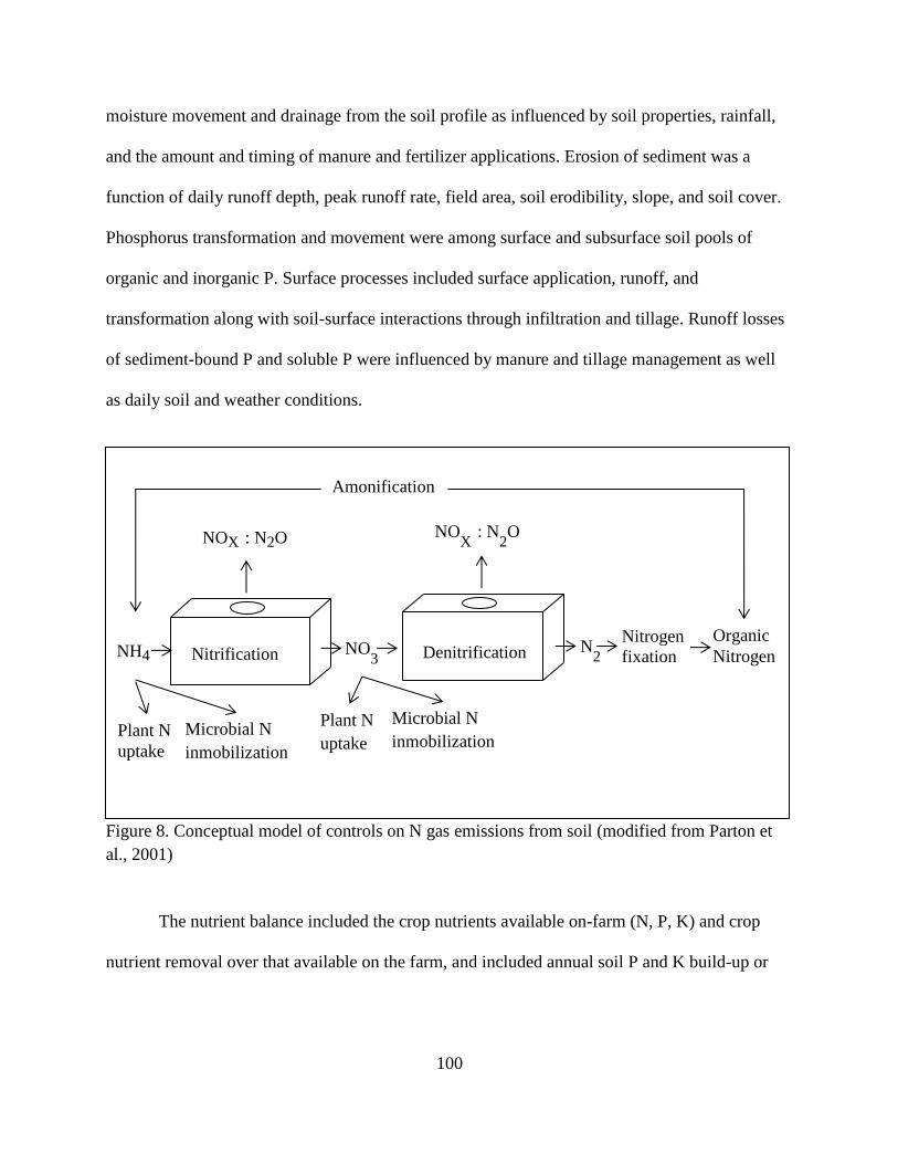
100
moisture movement and drainage from the soil profile as influenced by soil properties, rainfall,
and the amount and timing of manure and fertilizer applications. Erosion of sediment was a
function of daily runoff depth, peak runoff rate, field area, soil erodibility, slope, and soil cover.
Phosphorus transformation and movement were among surface and subsurface soil pools of
organic and inorganic P. Surface processes included surface application, runoff, and
transformation along with soil-surface interactions through infiltration and tillage. Runoff losses
of sediment-bound P and soluble P were influenced by manure and tillage management as well
as daily soil and weather conditions.
Figure 8. Conceptual model of controls on N gas emissions from soil (modified from Parton et
al., 2001)
The nutrient balance included the crop nutrients available on-farm (N, P, K) and crop
nutrient removal over that available on the farm, and included annual soil P and K build-up or
NOX : N2O NOX : N
2O
Nitrification Denitrification NH4 NO3 N
2
Nitrogen
fixation
Organic
Nitrogen
Amonification
Plant N
uptake
Microbial N
inmobilization
Plant N
uptake
Microbial N
inmobilization

101
depletion. Nutrient balance was influenced by the cropping system and the area designated for
each one (Table 22).
Table 22. Land area of five representative dairy production systems (ha)
Confine
Confine
AD
Seasonal
pasture
Seasonal pasture w
cash crop and AD
Annual
Pasture
Total land 111 111 111 809 111
Alfalfa area 36 36 10 10 40
Grass area 0 0 51 51 71
Corn area 75 75 51 374 0
Soybeans area 0 0 0 374 0
4.3.2. Confinement systems
4.3.2.1. On-farm nutrient cycling
On the confinement farms most of the nutrients were imported through purchased feed
(such as soybean meal, distillers grain, minerals and vitamins), fertilizer, and legume fixation.
Twenty-eight kilograms per hectare (25 lb/ac-yr) of nitrogen was applied to the corn at planting
time. To supply the N, P and K required by the corn, all manure was applied to land going to
corn production. The export of nutrients was through sales of milk, animals and feed, and losses
such as nitrogen volatilization, denitrification and leaching, and P and K loss through runoff.
There was also carbon loss as carbon dioxide, methane and through runoff.
Both confinement farms (with and without AD) had similar nutrient imports and exports,
nutrients available on-farm, nutrient crop removal, nutrients build-up or depletion (Table 23) and
nutrients loss (Table 24). When the AD was introduced there was a reduction in potassium
import because a portion of the bedding was recycled so less bedding was purchased.

102
Table 23. Annual nutrient cycling on five representative dairy farms.
Unit Confine
Confine
AD
Seasonal
pasture
Seasonal
pasture w cash
crop and AD
Annual
Pasture
Nutrients imported and exported
N imported kg/ha 195 195 326 212 342
N exported kg/ha 83 84 79 123 76
P imported kg/ha 12 12 23 16 22
P exported kg/ha 14 14 14 16 11
K imported kg/ha 26 15 72 41 52
K exported kg/ha 28 28 21 31 27
Nutrients available on farm
N kg/ha 298 293 479 235 500
P kg/ha 19 19 31 17 30
K kg/ha 108 97 193 59 195
Nutrients crop removal over that available on farm
N % 60 61 46 60 46
P % 115 117 76 105 64
K % 101 112 76 80 83
Nutrients build up or depletion
P build-up kg/ha 0 0 9.0 0 11.2
P depletion kg/ha 2.2 2.5 0 0.2 0
K build-up kg/ha 0 0 41.9 10.2 14.6
K depletion kg/ha 7.1 17.8 0 0 0
Table 24. Nutrient loss to the environment on five representative dairy farms (kg/ha-yr).
Confine Confine
AD
Seasonal
pasture
Seasonal
pasture w/cash
crop and AD
Annual
pasture
Nitrogen lost by volatilization 76.3 78.4 166 34.9 157
Nitrogen lost by leaching 12.1 11.1 51.3 11.5 19.4
Nitrogen lost by denitrification 8.1 7.2 40.6 6.7 12.2
Phosphorous loss in runoff and
leachate
0.34 0.34 0.22 0.56 0.00
Potassium loss through runoff 5.38 4.82 9.64 2.91 9.75
Carbon loss as carbon dioxide 6,194 6,044 5,380 8,857 7,869
Carbon loss as methane 209 189 250 31 197
Carbon loss through runoff 1.3 1.3 1.3 1.5 0.3

103
4.3.2.1.1. Potassium
Adding the AD on the confinement farm decreased the amount of K imported from 26
kg/ha-yr to 15 kg/ha-yr, and on-farm nutrient availability decreased from 108 kg/ha-yr to 97
kg/ha-yr (Table 23) because chopped straw bedding purchases decreased from 1.4 kg/cow-day to
0.5 kg/cow-day as a portion of the bedding was separated and recycled. Overall, K exports did
not change although there was a small decrease in K runoff related to the reduction in manure
volume with the AD digestate.
The land area available and crops produced were selected to provide the forage and corn
grain for the herd with only small amounts purchased or sold. The cropping system on the
confinement farm caused a small, long-term, K depletion (7.1 kg/ha-yr) which would require
periodic purchases of commercial K to correct. When the AD was added and less bedding was
imported the soil K depletion increased to 17.8 kg/ha-yr. This need for additional fertilizer would
offset a portion of the savings from the reduction in purchased bedding (Figure 9).
Figure 9. Soil phosphorous and potassium build up and depletion
-25-20-15-10-505
1015202530354045
Confine Confine AD Seasonal
pasture
Seasonal
pasture w
cash crop and
AD
Annual
Pasture
kg
/ha
-yr
P build up K build up
P depletion K depletion

104
4.3.1.1.2. Nitrogen
Nitrogen imported to farm was the same in both confinement farms (195 kg/ha-yr).
Nitrogen was mainly imported through purchased soybean meal and distillers grain. In addition
28 kg/ ha-yr (25 lb/ac-yr) of nitrogen was imported as fertilizer for corn land. Alfalfa and pasture
legumes imported N to the farm through N fixation. Perennial and forage legumes, such as
alfalfa and white clover may fix 280-560 kg of nitrogen per hectare (Lindemann and Glover,
2003). Nitrogen crop removal over that available on farm was 60%-yr, allowing between 293
and 298 kg/ha-yr of N available on farm (Table 23).
The export of N was through milk, animals, alfalfa silage and hay sold. Nitrogen also had
losses, most of all through volatilization (76.3 to 78.4 kg/ha-yr) that occurred in the barn, during
storage and field application (Table 24). There were also some losses through denitrification and
leaching which were related to soil properties and the amount and timing of manure and fertilizer
applications.
4.3.1.1.3. Phosphorus
Phosphorous imported to the farm was the same on both confinement farms (12 kg/ha-
yr). It was primarily imported through purchased soybean meal and distillers grain. Phosphorous
crop removal was between 115 and 117%-yr over that available on farm, allowing 19 kg/ha-yr of
P available on farm (Table 23). The export of P was through milk, animals, feed sold and losses
through runoff and leachate (0.34 kg/ha-yr) (Table 24). The low P available on farm and the
exports and losses produced a small P depletion between 2.2 and 2.5 kg/ha-yr (Table 23, Figure
9).

105
4.3.2.2 .Environmental emissions
Greenhouse gas emissions of carbon dioxide, methane, and nitrous oxide in addition to
ammonia and hydrogen sulfide originating from manure on the barn floor, the manure storage
structure and field applied manure were evaluated. The major emissions from each of the dairies
(from highest to lowest) were: methane, combustion carbon dioxide, ammonia, nitrous oxide,
hydrogen sulfide and, biogenic carbon dioxide (Table 25).
Table 25. Environmental emissions of five representative dairy production systems
Confine Confine
AD
Seasonal
pasture
Seasonal
pasture w cash
crop and AD
Annual
Pasture
Ammonia
Total farm (kg/yr) 10,340 10,619 22,436 35,068 21,234
Total farm (kg/ha-yr) 93 96 202 43 191
Hydrogen Sulfide
Total farm (kg/yr) 326 313 264 1,043 40
Total farm (kg/ha-yr) 2.9 2.8 2.4 1.3 0.4
Methane
Total farm (kg/yr) 31,001 28,062 37,192 37,582 29,174
Total farm (kg/ha-yr) 279 253 335 46 263
Nitrous Oxide
Total farm (kg/yr) 486 468 934 1,662 630
Total farm (kg/ha-yr) 4.4 4.2 8.4 2.1 5.7
Biogenic Carbon Dioxide
Net emission (kg/yr) -365,875 -357,925 -422,615 1,745,611 -347,118
Net emission (kg/ha-yr) -3,296 -3,225 -3,807 2,158 -3,127
Combustion CO2
Total farm (kg/yr) 35,683 30,210 29,864 20,371 24,093
Total farm (kg/ha-yr) 321 272 269 25 217
4.3.2.2.1. Carbon dioxide and methane emissions
Carbon loss as carbon dioxide was the greatest source of carbon loss in the total
confinement dairy systems. Ninety-five percent of the total carbon loss was lost as biogenic CO2

106
(Figure 10, Table 24) which was from plant, animal and microbial respiration from soil and
stored manure. Most of the biogenic carbon dioxide emissions originated in the housing facilities
from animal respiration and decomposition of organic matter in manure on floors in the barn
(Table 26). Confinement barn emissions were greater than the systems incorporating grazing
because of the extended period of time the animals were in the barn. When the AD was added
biogenic carbon dioxide emissions increased in manure storage (Table 26) because carbon
dioxide was released in the combustion of methane during anaerobic digestion. There was a
small decrease in biogenic carbon dioxide assimilated in feed because of the reduction in manure
during the digestion process. The result was a small decrease in biogenic carbon dioxide with the
AD.
Table 26. Biogenic carbon dioxide emissions of five representative dairy production systems
(kg/yr)
Confine Confine
AD
Seasonal
pasture
Seasonal
pasture w cash
crop and AD
Annual
Pasture
Housing facility 685,552 685,496 555,488 554,272 504,026
Manure storage 42,479 241,471 26,921 212,444 0
Assimilated in feed -1,093,905 -1,284,892 -1,249,702 734,613 -1,069,259
Grazing animal 0 0 244,678 244,282 218,114
Net emission -365,875 -357,925 -422,615 1,745,611 -347,118
Net emission (kg/ha-yr) -3,296 -3,225 -3,807 2,158 -3,127
Other major sources of CO2 emission were from fuel combustion (Table 25) related to
field operations such as tillage, planting, harvesting and other operations requiring
mechanization. Adding the AD lead to a 2% reduction in carbon loss as carbon dioxide and a 9%
reduction of carbon loss as methane. Each decrease was related to the conversion of methane to
biogas for electricity generation or water heating. The major source of methane was the long
term manure storage. Because the manure storage structure served as short-term storage to hold

107
manure before being deposited in the digester, carbon loss as methane decreased as the manure
storage period decreased (Table 24).
Major sources of methane emissions were from enteric fermentation and long term
manure storage with minor sources being in the barn floor and field applied manure. The dairy
cattle were the main source of methane emissions for each of the confinement dairies (Table 27).
The long term manure storage facility was also an important source of methane. The addition of
the anaerobic digester on the confinement farm decreased methane emission from the manure
storage structure by 26% (from 11,274 kg/yr to 8,360 kg/yr) by enclosing the manure in a tank
where the methane was converted to biogas (Table 27).
Table 27. Methane emissions of five representative dairy production systems (kg/yr)
Confine Confine
AD
Seasonal
pasture
Seasonal
pasture w cash
crop and AD
Annual
Pasture
Housing facility 19,690 19,661 20,115 20,238 19,497
Manure storage 11,274 8,360 7,070 7,118 0
Field application 38 40 71 203 39
Grazing 0 0 9,936 10,022 9,638
Total farm 31,001 28,062 37,192 37,582 29,174
Total farm (kg/ha-yr) 279 253 335 46 263
4.3.2.2.2. Ammonia emissions
Ammonia is produced when microbes breakdown protein and other nitrogen containing
compounds during decomposition causing an increase in pH (Hoeksema et al., 2012). In raw
manure there is a balance between ammonium concentration and volatile fatty acid concentration
which results in a pH near neutral. When volatile fatty acids are reduced during anaerobic
digestion, pH increases (Paul and Beauchamp, 1989) so pH is normally higher in digestate than
in raw manure. Volatile ammonia is formed (NH3), which could be up to 25% of the ammonium

108
fraction (Scottish Executive Environment and Rural Affairs Department, 2007). Most of the
ammonia emissions from the confinement farms originated from manure on the milking center
and barn floors, manure storage structures and following field application (Table 28). Because of
the increased volatility there was a small increase in ammonia emissions with AD.
Table 28. Ammonia emissions of five representative dairy production systems (kg/yr)
Confine Confine
AD
Seasonal
pasture
Seasonal
pasture w cash
crop and AD
Annual
Pasture
Housing facility 4,310 4,217 6,773 6,804 15,150
Manure storage 2,172 2,315 4,549 5,153 0
Field application 3,859 4,086 7,151 19,106 2,309
Grazing 0 0 3,963 4,005 3,774
Total farm 10,340 10,619 22,436 35,068 21,234
Total farm (kg/ha-yr) 93 96 202 43 191
4.3.2.2.3. Nitrous oxide emission
Nitrous oxide emissions originate primarily from nitrification and denitrification
processes in the soil, and also in the crust of the slurry manure storage (Rotz et al., 2011a).
Nitrous oxide has a global warming potential 298 times that of carbon dioxide, making it the
strongest of all greenhouse gas emissions in agricultural production (IPCC, 2007). Nitrous oxide
emissions can be greater where manure remains for longer periods where nitrification or
denitrification converts ammonium to nitrate or nitrate to atmospheric N2 (Figure 8) (IPCC,
2007).
On the confinement farms nitrous oxide emissions originated primarily in the housing
facilities, manure storage and farmland (Table 29). The pH of digested manure is typically higher
thereby supporting nitrous oxide reduction. The addition of an AD on the confinement farm
decreased the total farm emissions of nitrous oxide by a small amount (4%). Manure on the free

109
stall barn floor is typically a minor source of nitrous oxide emission (Rotz et al., 2011a) but some
enteric nitrous oxide could also be emitted by the animals (Hamilton et al., 2010).
Table 29. Nitrous oxide emissions of five representative dairy production systems (kg/yr)
Confine Confine
AD
Seasonal
pasture
Seasonal
pasture w cash
crop and AD
Annual
Pasture
Housing facility 204 198 339 375 325
Manure storage 147 143 243 269 0
Farmland 134 126 352 1,019 305
Total farm 486 468 934 1,662 630
Total farm (kg/ha-yr) 4.4 4.2 8.4 2.1 5.7
4.3.2.2.4. Hydrogen sulfide emissions
Hydrogen sulfide is a toxic compound that is regulated by the US EPA under the Clean
Air Act. Hydrogen sulfide is primarily created and emitted from decomposing manure under
anaerobic conditions (Rotz et al., 2011a). The major source of hydrogen sulfide on all dairies
was field application of manure (Table 30). On the confinement farms manure was stored under
anaerobic conditions beneath the crust formed on the manure surface which increased the
hydrogen sulfide emission. The anaerobic digester reduced hydrogen sulfide emissions by 4%
because of the recycled bedding and reduction of manure handled after the digestion process.
The confinement farm handled 3,155 t DM/yr of manure but when an anaerobic digester was
used the amount of manure handled was reduced to 3,102 t DM/yr.

110
Table 30. Hydrogen sulfide emissions of five representative dairy production systems (kg/yr)
Confine Confine
AD
Seasonal
pasture
Seasonal
pasture w cash
crop and AD
Annual
Pasture
Housing facility 35 34 30 29 39
Manure storage 63 61 50 49 0
Field application 228 218 184 964 0
Grazing 0 0 0 0 0
Total farm 326 313 264 1,043 40
Total farm (kg/ha-yr) 2.9 2.8 2.4 1.3 0.4
4.3.2.3. Environmental footprints
Environmental footprint is a measure of the demand on the ecosystem services of the
earth. Footprints were evaluated for water, reactive nitrogen, energy, and greenhouse gas
emissions. The footprints were determined by summing the estimates for each of the uses
(removing those allocated to co-products), and dividing by the amount of milk produced.
Water was mainly used for the production of feed crops, drinking water for animals,
animal cooling, cleaning of the parlor and holding areas on dairy farms. Reactive nitrogen is
essential in the growing of crops and feeding of animals. Primary losses of reactive nitrogen
include ammonia and nitrous oxide emissions to the atmosphere, nitrate leaching to ground
water, and the combustion of fuels. The energy footprint was the total energy required to produce
feed and milk which includes all fuel and electricity directly used in the production system as
well as the secondary energy used in the production of resources used on the farm. The carbon
footprint was determined as the net emission of the three GHG’s including all sources and sinks
of CO2, so a portion of the CO2 assimilated in the feed is in the carbon exported during feed,
milk, and animal productions.

111
4.3.2.3.1. Water footprint
In all dairies the major sources of water footprint were: feed production with rainfall,
followed by production of purchased feed and inputs (Table 31). There was a 28% reduction in
water use for purchased feed and inputs when the AD was used on the confinement farm because
of the reduction in purchased bedding. Because less bedding was purchased less water was
required for the production of bedding. Even though straw is a by-product of harvest it requires
water for growth.
Table 31. Water footprints of five representative dairy production systems
Unit Confine Confine
AD
Seasonal
pasture
Seasonal
pasture w
cash crop AD
Annual
Pasture
Feed production,
rainfall
t/yr 585,780 585,935 585,746 1,008,009 584,965
Drinking t/yr 2,810 2,810 4,193 4,185 3,977
Animal cooling t/yr 228 228 324 324 365
Parlor, equipment
cleaning
t/yr 913 913 1,296 1,295 1,460
Production of
purchased feed
and inputs
t/yr 128,317 92,701 326,354 328,487 335,579
Not allocated to
milk production
t/yr -122,454 -117,049 -160,046 -200,348 -144,650
Water footprint
with rainfall
kg/kg
FPCM-yr
600 569 630 905 716
Water footprint
without rainfall
kg/kg
FPCM-yr
99 68 195 170 244
Water footprint w
rainfall per ha
kg/kg
FPCM-
ha-yr
5.4 5.1 5.7 1.1 6.4
The water footprint decreased 4% with AD evaluated as the water footprint not allocated
to milk production (Table 31). Water used in the production of machinery, fertilizer, pesticides,
and plastic was considered to be insignificant (Rotz et al., 2011a). Water use for drinking, animal
cooling and parlor and equipment cleaning on all farms increased with the number of cows.

112
4.3.2.3.2. Energy footprint
The major sources of energy use footprint were production of resource inputs, milking
and milk cooling, feed production, animal feeding, manure handling and animal housing
ventilation and lighting (Table 32). The confinement farms had the highest energy use in feed
production (215,987 MJ/yr) because it produced 36 to 54% more feed than the seasonal and
annual pasture farms. Because animals were kept in the barn all year, animal feeding (152,438
MJ) and animal housing ventilation and lighting (57,779 MJ/yr) were also the greatest energy
demands of all the farms (Table 32).
Table 32. Energy footprint of five representative dairy production systems
Unit Confine Confine
AD
Seasonal
pasture
Seasonal
pasture w
cash crop
AD
Annual
Pasture
Feed production MJ 215,987 215,862 141,373 190,568 115,236
Animal feeding MJ 152,438 151,968 122,344 120,557 110,996
Manure handling MJ 74,329 64,052 67,626 256,978 68,338
Milking, milk
cooling
MJ 232,312 155,099 267,928 179,039 228,576
Animal housing
ventilation, lighting
MJ 57,799 57,799 56,576 56,444 18,091
Production of
resource inputs
MJ 1,906,139 1,249,329 2,159,025 2,478,746 2,033,489
Not allocated to
milk production
MJ -451,019 -338,499 -533,488 -571,014 -434,975
Energy footprint MJ/kg
FPCM
2.2 1.6 1.9 2.1 2.0
Energy footprint
per ha
MJ/kg
FPCM-ha
0.02 0.01 0.02 0.003 0.02
Adding the AD on the confinement dairy reduced energy use for manure handling by
14% (10,277 MJ/yr), by reducing the volume of bedding handled and applied as manure. Energy
for milking and milk cooling was reduced by 33% (77,213 MJ/yr) as energy for water heating
was partially replaced by biogas from the digester. The greatest reduction of the energy footprint

113
was from the reduction in fossil fuel energy used to generate electricity off-farm (production of
resource inputs) which was reduced 34% (656,810 MJ/yr). There was also a 25% decrease in
energy use not allocated to milk production (allocated to the cattle growth and sold as beef).
4.3.2.3.3. Reactive nitrogen loss footprint
The primary sources of reactive nitrogen loss were ammonia emissions, nitrate leaching,
nitrous oxide emissions fuel combustion emissions and production of resource inputs (Table 33).
Reactive nitrogen is essential to crop and livestock production. The confinement dairy had the
smallest reactive nitrogen loss footprint (8.9 g/kg FPCM-yr) (Table 33) because it had the least
ammonia emissions, nitrate leaching, nitrous oxide emissions and nitrogen loss during the
production of resource inputs. Each of these (except ammonia) was reduced when the AD was
used on the confinement farm. Ammonia emissions increased because the pH increased in the
digestate, thereby producing more ammonium in the volatile form. Nitrate leaching decreased
because less manure was being applied to the land. Nitrous oxide emissions decreased because
the higher pH in the digestate allowed nitrous oxide reduction from ammonium or nitrate to
nitrous oxide.
Nitrous oxide emissions due to fuel combustion were also reduced on the confinement
farm with AD because less manure was being handled (Table 33). Combustion of fossil fuel
releases nitrogen oxides to the atmosphere which increase with field operations that require more
tillage, planting and harvesting.

114
Table 33. Reactive nitrogen loss footprint of five representative dairy production systems
Unit Confine Confine
AD
Seasonal
pasture
Seasonal
pasture w
cash crop AD
Annual
Pasture
Ammonia em[a] kg 8,496 8,725 18,439 57,912 17,447
Nitrate leaching kg 1,343 1,239 5,711 19,234 2,164
Nitrous oxide em kg 309 297 594 2,165 401
Fuel combustion
em
kg 118 100 94 644 76
Production of
resource inputs
kg 428 352 1,052 1,941 1,135
Not allocated to
milk production
kg -1,825 -1,827 -3,690 -10,617 -3,045
Reactive nitrogen
footprint
g/kg
FPCM
8.9 8.9 18.5 30.1 16.7
Reactive nitrogen
footprint per ha
g/kg
FPCM-ha
0.1 0.1 0.2 0.04 0.1
[a]: em= emission
4.3.2.3.4. Carbon footprint
The carbon footprint measures total GHG emissions expressed in CO2 equivalent units
(CO2e). The primary contributors to the carbon footprint were animal emissions (25 to 59% of
total GHG), manure emissions (9 to 34% of total GHG), production of resource inputs (9 to 23%
of total GHG), emissions during feed production (2 to 7% total GHG) and fuel combustion
emissions (1 to 3% of total GHG) (Table 34).
The confinement dairies had the lowest animal emissions because animal respiration was
based on daily intake of feed dry matter (Rotz et al., 2011a). Because animals in confinement
consume less forage in the diet than grazing animals, carbon dioxide emissions decreased. When
using an AD, carbon dioxide emissions from manure decreased because methane emissions were
reduced by containing all manure in a closed tank where it was converted biogas. The carbon

115
footprint associated with the production of resource inputs decreased by 31% because of the
reduction of fossil fuel used to generate electricity off-farm.
Table 34. Carbon footprint of five representative dairy production systems
Unit Confine Confine
AD
Seasonal
pasture
Seasonal
pasture w
cash crop AD
Annual
Pasture
Animal em[a] kg 481,602 481,395 741,392 1,493,521 716,839
Manure em kg 397,334 321,179 360,953 766,547 108,683
Emission during
feed production
kg 35,444 33,248 96,815 132,907 82,809
Net biogenic carbon
dioxide em
kg -365,550 -357,610 -422,188 2,928,001 -346,810
Fuel combustion em kg 35,652 30,184 29,837 40,706 24,072
Production of
resource inputs
kg 206,787 142,209 263,018 537,109 278,397
Not allocated to
milk production
kg -193,915 -171,407 -244,488 -489,918 -191,363
Carbon footprint
without biogenic
CO2
kg/kg
FPCM
0.97 0.84 1.04 1.00 0.93
Carbon footprint
with biogenic CO2
kg/kg
FPCM
0.66 0.54 0.72 2.10 0.65
Carbon footprint
with biogenic CO2
per ha
kg/kg
FPCM-
ha
0.006 0.005 0.006 0.003 0.006
[a]: em= emission
4.3.3. Seasonal pasture farms
4.3.3.1. On-farm nutrient cycling
Most of the nutrients were imported on the seasonal pasture dairies were from purchased
feed (such as hay, soybean meal, distillers grain, and minerals and vitamins), fertilizer, manure
application and forage legume nitrogen fixation. All manure collected in the milking parlor and
barn was applied to land going to corn production and twenty-eight kilograms per hectare (25
lb/ac) of commercial nitrogen fertilizer was applied to corn at planting time. Nitrogen from
legumes and manure applied by the grazing animals supplied the nutrients for the grass pasture.

116
The exports of nutrients were through milk, animals and feed sold. Ten percent of the
feed produced on the seasonal farm was sold and it was increased to 87% when additional land
was acquired to accommodate the additional manure required for the AD. Some nutrients were
the lost to the environment through nitrogen volatilization, denitrification, leaching, and loss of
phosphorous and potassium through runoff. There were also carbon losses leaving the farm as
carbon dioxide, methane or through runoff.
Nutrient cycling was different on the seasonal pasture farms because the land use and
cropping system was different. The seasonal pasture had a 111 ha land base which expanded to
809 ha when cash crops were produced (Table 22).
4.3.3.1.1. Potassium
The seasonal pasture had the greatest soil potassium build up (41.9 kg/ha-yr) (Figure 9).
Potassium imports (72 kg/ha-yr) (Table 23) were from the purchase of 13 t of hay (Table 20)
following the shift of 26 ha of land for alfalfa production to land for grazing animals (Table 22).
Potassium was also imported with purchase of chopped straw for bedding which contained
nitrogen, phosphorous and potassium (Shaver and Hoffman, 2010). The seasonal farm also
exported less potassium (21 kg/ha-yr), allowing potassium availability on-farm of 193 kg/ha-yr.
The seasonal farm with an expanded land base for cash crop production and AD had
greater K exports (compared to the other farms) because 87% of the total crop production was
sold (Table 23). The increase in pasture land also decreased potassium loss to the environment
(Table 24).
4.3.3.1.2. Nitrogen
The seasonal pasture dairy imported more nitrogen per unit area than the seasonal farm
with AD and additional land for cash crop production (Table 23) because relatively more

117
bedding and feed were purchased. A greater percentage of the land was in alfalfa and
grass/legume production, thereby increasing nitrogen import by fixation.
Figure 10. Nutrients available on farm
Figure 11. Nutrients crop removal over that available on farm.
-50
50
150
250
350
450
550
Confine Confine AD Seasonal
pasture
Seasonal
pasture w
cash crop and
AD
Annual
Pasture
kg/h
a
Nitrogen available on farm
Phosphorous available on farm
0
20
40
60
80
100
120
140
Confine Confine AD Seasonal
pasture
Seasonal
pasture w
cash crop and
AD
Annual
Pasture
%
N crop removal over that available on farm
P crop removal over that available on farm
K crop removal over that available on farm

118
The seasonal pasture dairies had the greatest nitrogen loss to the environment (258 kg/ha-
yr). The losses were from leaching (51 kg/ha-yr), denitrification (40.6 kg/ha-yr) and
volatilization (166 kg/ha-yr) (Figure 12). Denitrification and leaching losses from the soil were
related to the rate of moisture movement and drainage from the soil profile as influenced by soil
properties, rainfall, and the amount and timing of manure and fertilizer applications. There was
more nitrogen loss by leaching because the urine deposited in the pasture had high
concentrations of nitrogen which could exceed plant uptake (Table 24).
Nitrogen lost through volatilization was the greatest source of loss on all the dairies
(Figure 12). Nitrogen is the most abundant nutrient in manure and the seasonal pasture dairy had
the highest nitrogen lost by volatilization (166 kg/ha-yr) (Table 24) because of losses from
manure in the barn, milking parlor, during land application and from the urine and manure
deposited by the cattle.
On a unit area basis, nitrogen losses were reduced by 79% on the seasonal pasture with
cash crop and AD compared to the seasonal pasture dairy (Figure 12, Table 24). Because of the
increased land for cash crop production more nitrogen was used for crop production compared to
that available on-farm.
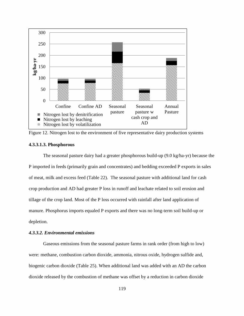
119
Figure 12. Nitrogen lost to the environment of five representative dairy production systems
4.3.3.1.3. Phosphorous
The seasonal pasture dairy had a greater phosphorous build-up (9.0 kg/ha-yr) because the
P imported in feeds (primarily grain and concentrates) and bedding exceeded P exports in sales
of meat, milk and excess feed (Table 22). The seasonal pasture with additional land for cash
crop production and AD had greater P loss in runoff and leachate related to soil erosion and
tillage of the crop land. Most of the P loss occurred with rainfall after land application of
manure. Phosphorus imports equaled P exports and there was no long-term soil build-up or
depletion.
4.3.3.2. Environmental emissions
Gaseous emissions from the seasonal pasture farms in rank order (from high to low)
were: methane, combustion carbon dioxide, ammonia, nitrous oxide, hydrogen sulfide and,
biogenic carbon dioxide (Table 25). When additional land was added with an AD the carbon
dioxide released by the combustion of methane was offset by a reduction in carbon dioxide
0
50
100
150
200
250
300
Confine Confine AD Seasonal
pasture
Seasonal
pasture w
cash crop and
AD
Annual
Pasture
kg/h
a-y
r
Nitrogen lost by denitrification Nitrogen lost by leaching Nitrogen lost by volatilization
120
emission (20,371 kg/yr) from soil respiration. The major emissions from this farm were biogenic
carbon dioxide (1,745,611 kg/yr) from the combustion of biogas (Table 25).
4.3.3.2.1. Carbon dioxide and methane emissions
The seasonal pasture with additional land for cash crop production and AD had the
greatest carbon loss as carbon dioxide (8,857 kg/ha-yr) (Table 24) because any remaining biogas
that was not used for either electricity generation or water heating was burned off in a flare.
Most of the biogenic carbon dioxide emissions on the seasonal pasture farm were from
housing facilities related to animal respiration and manure on floors in the barn (Table 26). The
grazing animals also increased biogenic carbon dioxide emissions (Table 26) because animal
respiration was based on daily intake of feed dry matter (Rotz et al., 2011a). Because grazing
animals consumes higher forage diets, carbon dioxide emission increased.
The greatest biogenic carbon dioxide emissions in the seasonal pasture with expanded
cash crop and AD farm was because of the assimilation in feed due to the increased crop land.
Croplands usually assimilate C from CO2 in the atmosphere, but also emit CO2 through plant
(autotrophic) and soil (heterotrophic) respiration (Chianese et al., 2009a). Biogenic carbon
dioxide emission in manure storage increased also increased in this farm (Table 26) because this
emission includes the carbon dioxide created through combustion of methane.
The seasonal pasture with cash crop production and AD had the lowest carbon loss as
methane (31 kg/ha-yr). Major sources of methane included long term storage and because
storage time was reduced by holding the manure for a short time before placing it in the digester
carbon loss as methane decreased (Table 24). The seasonal pasture farms had greater housing
methane emissions than the confinement farm because grazing cows consumed more forage. The

121
enteric methane emissions per cow increase with the percentage of fiber that was fed in the diet
cow (Chianese et al., 200c).
Grazing animals in seasonal and annual pasture dairies increased methane emissions
(9,630 to 10,022 kg/yr) because of the excreted feces and urine that were deposited on pastures
(Table 27). Some studies have shown that feces are a small but significant source of methane and
that emissions from urine are similar to background soil emissions (Jarvis et al., 1995; Yamulki
et al., 1999).
4.3.3.2.2. Ammonia emissions
Ammonia emissions (22,436 kg/yr) from the seasonal pasture dairy were more than
double that of the confinement farms (Figure 13, Table 28). Emissions from the housing
facilities, manure storage and field application increased because there were more animals in the
seasonal pasture system (142-cows) than the confinement system (100-cows), therefore more
manure and urine was produced in these farms.
Figure 13. Ammonia emissions of five representative dairy production systems
0
5000
10000
15000
20000
25000
30000
35000
40000
Confine Confine AD Seasonal
pasture
Seasonal
pasture w
cash crop
and AD
Annual
Pasture
kg/y
r
Ammonia
Grazing Field application
Manure storage Housing facility

122
The seasonal pasture with additional land for cash crop production and AD had the
greatest ammonia emissions (35,068 kg/yr) because of the amount of manure applied to field
(Figure 13, Table 28). Also, there was an increase in ammonia emissions as a result of the
anaerobic digestion process due to an increase in slurry ammonium-N content.
4.3.3.2.3. Nitrous oxide emissions
The seasonal pasture with additional land for cash crop production and AD had the
greatest emission of nitrous oxide (1,662 kg/yr) because of the additional nitrogen input on the
additional crop land which increased farmland emissions (1,019 kg/yr) (Figure 14, Table 29).
Figure 14. Nitrous oxide emissions of five representative dairy production systems.
The seasonal pasture with cash crops and AD had greater nitrous oxide emissions in the
housing facilities (375 kg/yr). Nitrous oxide emissions can be greater where manure remains for
longer periods as in the grazing areas. Manure on the floor of free stall barns appears to be a
0
200
400
600
800
1000
1200
1400
1600
1800
Confine Confine AD Seasonal
pasture
Seasonal
pasture w
cash crop
and AD
Annual
Pasture
kg/y
r
Nitrous oxide
Farmland
Manure storage
Housing facility

123
negligible source of nitrous oxide emission (Rotz et al., 2011a), but a small amount of enteric
nitrous oxide is emitted by the animals (Hamilton et al., 2010) (Table 29).
Nitrous oxide emissions from the manure storage were from the natural crust that was
formed on the stored slurry (Chianese et al., 2008b). The seasonal pasture dairies released more
nitrous oxide (243 to 269 kg/yr) than the confinement dairies (143 to 147 kg/yr) (Table 29)
because manure was collected less frequently during grazing season than in confinement storage.
4.3.3.2.4. Hydrogen sulfide emissions
The seasonal farm with AD and cash crops had the greatest hydrogen sulfide emissions
(1,043 kg/yr) (Figure 15, Table 30). The major source of hydrogen sulfide was land application
of manure (184 to 964 kg/yr). The seasonal pasture dairy had the lowest emissions from field
application (184 kg/yr) because less manure was collected and applied to the field. The seasonal
pasture with cash crops and AD emitted more hydrogen sulfide during field application (964
kg/yr) because: 1) The manure had been in anaerobic conditions (due to the anaerobic digester),
encouraging the transformation from sulfide to hydrogen sulfide, and 2) since there was more
crop land, more manure was applied on the soil, leading to more emissions.

124
Figure 15. Hydrogen sulfide emission of five representative dairy production systems.
4.3.3.3 Environmental footprints
Water, reactive nitrogen, energy use and greenhouse gas emission footprints were
evaluated for the seasonal pasture dairies.
4.3.3.3.1. Water footprint
The primary measures of the water footprint were rainfall for feed production followed
by production of purchased feeds and inputs (Table 31). The seasonal pasture with additional
land for cash crops and AD had the greatest water footprint (905 kg/kg FPCM-yr) due to feed
production (sold and consumed) because this dairy had more area for crop production compared
to the other dairies (Table 31). The dairy had less water footprint not allocated to milk
production (-200,348 t/yr) because the cash crops sold were considered to be exported from the
farm. Water used in the production of machinery, fertilizer, pesticides, and plastic was not
significant (Rotz et al., 2011a). Water use for drinking, animal cooling and parlor and equipment
0
200
400
600
800
1000
1200
Confine Confine AD Seasonal
pasture
Seasonal
pasture w
cash crop
and AD
Annual
Pasture
kg/y
r Hydrogen sulfide
Field application
Manure storage
Housing facility

125
cleaning was the same for both seasonal farms because it was based on the number of cows
(Table 31).
4.3.3.3.2. Energy footprint
The transition from a confinement to a seasonal pasture dairy reduced the energy
footprint by 14%. There was a reduction of 35% in on-farm feed production, 20% in animal
feeding and 8% in manure handling (Table 32). These reductions were related to the shift of 24
ha of corn production to grazing. There was an 18% decrease in energy not allocated to milk
production, which was allocated to the cattle growth produced and sold as beef. This was
influenced by the relative quantities of milk and cattle sold.
The seasonal pasture with additional land for cash crops and AD dairy had the greatest
energy use footprint for production of resources inputs (2,478,746 MJ/yr), such as fuel,
electricity, machinery, fertilizer, pesticides, seed, and plastic for the additional land for cash
crops. The farm also had the greatest energy footprint for manure handling related to the 12,882
wet t/yr of imported manure. However, the seasonal pasture with cash crops and AD dairy had
4% less energy use footprint 2.1 MJ/kg FPCM-yr (fat and protein corrected milk, 4% fat and
3.3% protein) compared to the confinement dairy (2.2 MJ/kg FPCM-yr) which had less area for
crop production and an energy use for production resource inputs of 1,906,139 MJ/kg FPCM-yr
(Table 32). The decrease in energy footprint was for two reasons: 1) the addition of the anaerobic
digester and 2) because the seasonal pasture farm required less energy for feed production and
animal feeding than the confinement farm. The addition of the AD on the seasonal farm reduced
energy use by 23% (compared to the confinement farm) for milking, milk cooling and water
heating. Energy for animal feeding was reduced by 21% and 12% for feed production compared
to confinement because of the addition of grazing.

126
4.3.3.3.3. Reactive nitrogen loss footprint
The seasonal pasture dairy with cash crops and AD had the greatest reactive nitrogen loss
footprint because of ammonia (57,912 kg/yr), nitrate leaching (19,234 kg/yr), nitrous oxide
(2,165 kg/yr), production of resource inputs (1941 kg/yr) and fuel combustion emissions (644
kg/yr). Ammonia emissions were higher because more manure was applied (due to the imported
manure). Also, there was an increase in ammonia emissions as a result of the anaerobic
digestion process. Nitrate leaching, nitrous oxide, combustions emissions and production of
resource inputs were increased because of the increased land for cash crop. Combustion of fossil
fuels leads to the creation of nitrogen oxides in the atmosphere which increases with field
operations that require more tillage, planting and harvesting.
4.3.3.3.4. Carbon footprint
The seasonal pasture with additional land for cash crops and AD had the greatest carbon
footprint (2.10 kg/kg FPCM-yr) because of biogenic carbon dioxide, which accounted for 50%
of the total GHG emissions. This farm also had the highest animal and manure emissions
compared to the other dairies (Table 34) because of the 12,882 t/yr of imported manure.
Emissions during feed production, fuel combustion and production of resource inputs were also
higher due to the expanded land base for cash crop production (Table 34).
4.3.4. Annual Pasture-based farm
4.3.4.1. On-farm nutrient cycling
Most of the nutrients on the annual pasture-based farm were imported through purchased
feed (such as hay, soybean meal, distillers grain and minerals and vitamins) and nitrogen fixation
by alfalfa and legumes in the grass/legume pasture. Nitrogen from legumes and manure applied
by the grazing animals supplied the nutrients for the grass pasture. Eighty percent of manure

127
collected in the milking parlor was applied to grass and 20% to the alfalfa land. Nutrient exports
were through milk, sales of animals and feed (10% of feed produced was sold), nitrogen
volatilization, denitrification and leaching, and loss of phosphorous and potassium through
runoff. There were also carbon losses leaving the farm as carbon dioxide, methane or through
runoff.
4.3.4.1.1. Potassium
Potassium imports (52 kg/ha-yr) (Table 23) were mostly from the purchase of 114 t/yr of
dry grain (Table 20) following the shift of land for crop production to land for grazing animals
(Table 22). Grains contain less K than do legumes (forages contain 1-3% K; grain contains 0.5-
0.8% K) (Dupchak, 2001), that is why the annual pasture (which purchased dry grain) had less
potassium imported than the seasonal farm (which purchased hay and no dry grain).
4.3.4.1.2. Nitrogen
The annual pasture-based dairy had more nutrients available on-farm (500 kg/ha-yr) than
the seasonal pasture farm (Table 23, Figure 10), because more N was imported through legumes
fixation and purchased feed and less N was exported because this farm did not had grain
production.
The annual pasture-based dairy had higher nitrogen loss from volatilization (157 kg/ha-
yr) and leaching (12.2 kg/ha-yr) than the confinement dairy because the deposited urine could
exceed the uptake by plants (Table 24).
4.3.4.1.3. Phosphorous
The annual pasture-based dairy had the greatest soil phosphorus build up (11.2 kg/ha-yr)
(Figure 9) because beside it was the only farm that had application of manure collected on grass,
also there were more imported feeds (primarily grain and concentrates) and less phosphorous

128
was exported through crops that were sold as compared to the other farms (Table 23). This farm
did not have P loss in runoff because of the permanent vegetative cover that reduced runoff and
erosion (Table 24).
4.3.4.2. Environmental emissions
4.3.4.2.1. Carbon dioxide and methane emissions
The annual pasture-based dairy had the second greatest carbon loss as carbon dioxide
(7,869 kg/ha-yr) because it had the greatest production of hay (Table 24). Large stacks of hay
stored under cover goes through a heating process during the first few weeks of storage. Heating
occurs due to the respiration of microbial organisms in the hay. Through respiration,
carbohydrates in the plant tissue and oxygen are converted to carbon dioxide, water, and heat
(Rotz et al., 2011a). This farm also had the lowest carbon loss through runoff (0.3 kg/ha-yr)
because of the permanent vegetative cover.
The annual pasture-based farm had biogenic carbon dioxide emissions in the housing
facility similar to the seasonal pasture farm (Table 26). Even though the annual pasture did not
have housing facilities, biogenic carbon dioxide emissions were produced in the milking parlor
by animal respiration and manure on the floor. This farm had less assimilation in feed than the
seasonal farm because it did not produce corn. Also, biogenic carbon dioxide released by the
grazing animals increased (Table 26) compared to the confinement farm because the animals
consumed higher forage diets.
Methane emissions on the annual pasture-based farm were similar to the confinement
farm. Even though the annual pasture only had a milking parlor as cow housing, similar methane
emissions due to enteric fermentation (19,497 kg/yr) were produced because grazing cows
129
consume more forage. Also, this farm did not have methane emissions from manure storage
because this farm stacked the manure and applied to land daily.
4.3.4.2.2. Ammonia emissions
The annual pasture-based farm had more than twice the ammonia emissions (21,234
kg/yr) as the confinement farm (Table 28). Housing facilities emissions increased (15,150 kg/yr)
because there were more animals in annual pasture (160-cows) compared to the confinement
(100-cows), therefore more manure and urine was produced in this farm (Table 28, Figure 13).
The manure on the milking center floors produced more ammonia than the urine deposited on
pasture (3,774 kg/ha-yr). Ammonia emission due to field application was lower in the annual
pasture-based dairy (2,309 kg/yr) because less manure was collected and consequently less was
applied on the field (2,599 t DM/yr).
4.3.4.2.3. Nitrous oxide emissions
The annual pasture-based and seasonal pasture farm had similar nitrous oxide emissions
from farmland (Table 29, Figure 14) because manure remained for longer periods in the grazing
areas and the annual pasture farm did not have manure storage.
4.3.4.2.4. Hydrogen sulfide emissions
The annual pasture did not have hydrogen sulfide emissions in manure storage or field
application because the manure was applied daily (Table 30, Figure 15). Without long term
manure storage under anaerobic conditions only small amounts of sulfide could be formed. The
manure in the milking parlor produced 39 kg/yr of hydrogen sulfide.

130
4.3.4.3 Environmental footprints
4.3.4.3.1. Water footprint
The annual pasture-based farm had the second greatest water footprint (716 kg/kg FPCM-
yr) due to purchased feed and inputs (335,579 t/yr) because 41% of the animal feed consumed
was purchased and required more animal and milking supplies, because it had more cows. Water
use for drinking, animal cooling and parlor and equipment cleaning was higher for the annual
pasture-based farm because it had the greatest number of cows (Table 31).
4.3.4.3.2. Energy footprint
The transition from confinement to an annual pasture-based farm reduced the energy
footprint by 11%. This decrease was because of a reduction of 47% in feed production, 27% in
animal feeding and 9% in manure handling (Table 32). There was also a decrease of 4% in
energy not allocated to milk production which was allocated to the cattle weight produced and
sold as beef. Additionally, the annual pasture farm had a 69% decrease in energy for animal
housing and ventilation compared to the confinement farm because cattle were on pasture or
open lots throughout the year.
The annual pasture had a greater energy use footprint for production of resources inputs
(2,033,489 MJ/yr) because it purchased 41% of the feed for the animals. The 27% reduction in
animal feeding and 47% reduction for feed production on the annual pasture-based farm
compared to the confinement farm was because of the shift of crop land to grazing land and,
consequently, the addition of grazed forage in the diet of the cattle.
The seasonal and annual pasture dairies required less energy for manure handling because
manure was only collected from the milking parlor and from the barn (for the seasonal pasture).
The annual pasture-based dairy has higher energy required for manure handling (68,338 MJ/yr)

131
compared to the seasonal pasture (67,626 MJ/yr) because it hauls manure daily, increasing
machinery use and fuel (Table 32).
4.3.4.3.3. Reactive nitrogen loss footprint
The annual pasture-based dairy had a 10% lower reactive nitrogen loss footprint than the
seasonal farm because ammonia and nitrous oxide emissions, nitrate leaching, fuel combustion
and footprint not allocated to milk production were lower (Table 33). Ammonia decreased
because this farm did not have a housing facility where manure could produce emissions. Nitrous
oxide emissions were less than the seasonal pasture farm because the annual pasture-based farm
did not have manure storage. Fuel combustion emission and nitrate leaching were lower than the
seasonal farm because the farm only had land for grazing and no crop production. The footprint
not allocated to milk production decreased because it was allocated to the cattle weight gain
produced and sold as beef. The footprint from the production of resource inputs increased
because the annual pasture-based farm purchased 8% more or feed than the seasonal farm (Table
33).
4.3.4.3.4. Carbon footprint
The annual pasture-based farm had a carbon footprint similar to the confinement farm
(Table 34). Animal, feed production and production of resource inputs emissions were similar to
the seasonal pasture. However, the annual pasture-based farm had the lowest manure carbon
footprint (108,683 kg/yr) because there was no manure storage or housing facilities and the
primary source of emissions of carbon dioxide were from the decomposition of organic matter
in manure deposited by animals in the floor of the milking parlor.

132
CHAPTER 5: CONCLUSIONS
Five representative dairy production systems were compared to evaluate resource use and
conservation, economic and environmental impacts in the transition from total confinement to
seasonal-and annual-pasture based systems. The available land base on four farms was held
constant at 111 ha, which was the area needed to support 100 large Holstein cows plus
replacements with small annual shortage or excess of feed, and a near-balance of phosphorous
and potassium from manure cycling on the farm. The land base of a seasonal pasture system was
expanded to 809 ha to provide additional land for cash crop production and land application of
imported manure used to operate an anaerobic digester. Anaerobic digestion was evaluated on
the confinement and seasonal pasture dairies.
1. Based on a whole-farm nutrient balance, the 111 ha land base supported 100 large-frame
(726 kg) Holsteins cows on the total confinement farm, 142 medium-frame (590 kg) cows on
the seasonal pasture dairy, and 160 small-frame (454 kg) New Zealand type cows with
replacements on the annual pasture dairy.
2. The annual pasture-based system had the greatest net return to management and unpaid
factors followed by the seasonal pasture and confinement systems. Compared to the total
confinement system, net income on the annual pasture increased 20% and 17% on the
seasonal pasture.
3. The addition of an anaerobic digester on the 100-cow total confinement dairy decreased the
net return to management and unpaid factors by 15%.
4. When anaerobic digestion was added to the seasonal pasture with an increased land base for
cash crop production and an imported manure volume equivalent to a 500-cow dairy, the net

133
return to management and unpaid factors increased 388% compared to the seasonal dairy
alone. Facility and structure costs increased 108%, manure handling and related labor costs
increased 302%, but bedding costs decreased 67% and energy costs decreased 34%. Net
purchased feed and bedding costs decreased 761% mainly because of the sale of cash crops;
therefore AD on the seasonal farm was primarily paid for from the sales of cash crops.
5. Nitrogen, phosphorous and potassium were imported primarily through purchased feed and a
small amount (28 kg/ha) of commercial N applied to corn at planting. The primary source of
N was fixation by alfalfa and other legumes in the grass/ legume pasture. Nutrient exports
were from milk, meat and feed sales, nutrients lost to the environment by volatilization,
leaching, and runoff. The corn/alfalfa rotation on the confinement dairy led to an annual
depletion of soil P (2.2 kg/ha-yr) and K (7.1 kg/ha-yr). The seasonal pasture cropping system
led to a build-up of P (9 kg/ha-yr) and k (41.9 kg/ha-yr) while the annual pasture led to a P
build-up of 11.2 kg/ha-yr and K build-up of 14.6 kg/ha/yr.
6. The addition of an anaerobic digester on the confinement farm increased K depletion in the
cropping system (from 7.1 to 17.8 kg/ha-yr) because a portion of the chopped straw bedding
was separated and recycled, thereby reducing the amount of K imported in the purchased
bedding.
7. There was 68% more N available on the annual pasture dairy and 61% more N available on
the seasonal pasture dairy than was available on the confinement farm. Of the N imported to
the confinement dairy (195 kg/ha-yr), 39% was lost by volatilization, 6% by leaching and 4%
by denitrification. Of the N imported to the seasonal dairy (326 kg/ha-yr) 51% was lost to
volatilization, 16% to leaching and 12% to denitrification. The annual pasture imported 342
kg/ha-yr and lost 46% to volatilization, 6% to leaching and 4% to denitrification.
134
8. There was little difference in nitrogen, phosphorus, potassium and carbon loss to the
environment from anaerobic digestion.
9. On the seasonal pasture, compared to confinement, emissions of ammonia increased 117%,
nitrous oxide 92%, methane 20% and biogenic carbon dioxide 16%. Emissions of hydrogen
sulfide decreased 19% and combustion CO2 decreased 16%.
10. On the annual pasture, compared to confinement, ammonia emissions increased 105% and
nitrous oxide 30%. Hydrogen sulfide decreased 88%, combustion CO2 decreased 32%,
methane decreased 6% and biogenic carbon dioxide decreased 5%.
11. On the seasonal pasture, compared to confinement, the water use footprint increased 5% and
in the annual pasture increased 19% because of an increase in purchased feed and an increase
in number of cows.
12. On the seasonal pasture, compared to confinement, the energy footprint decreased 14% and
decreased 9% in the annual pasture due to a reduction in on-farm feed production, animal
feeding and manure handling related to the shift from corn production to grazing land.
13. On the seasonal pasture, compared to confinement, carbon footprint increased 9% because
animal and feed production emissions increased due to an increase in number of animals and
forage intake. The annual pasture dairy had a 2% decrease in carbon footprint because of a
decrease in manure emissions and fuel combustion.
14. On the seasonal pasture, compared to confinement, the reactive nitrogen footprint increased
108% and the annual pasture reactive nitrogen footprint increased 86% because of an
increase in production of resource inputs and ammonia emission. In addition, the seasonal
pasture had a higher nitrogen footprint because of an increase of 325% on nitrate leaching.

135
15. When the land base on the seasonal pasture was increased with manure imported to maintain
the digester the water footprint increased 44%, reactive nitrogen footprint increased 63%, the
energy footprint 11% and the carbon footprint 192% compared to the seasonal dairy alone.
136
CHAPTER 6: SUGGESTIONS FOR FUTURE RESEARCH
Since one of the limitations was to integrate an anaerobic digester into a small-scale farm
with imported manure, is important to validate the procedure performed for this study using
IFSM model by comparing results with actual farm records.
Pasture-based dairy farms are gaining popularity, because of the economic benefits. There is
a need to collect more information related to confinement-winter/pasture-summer and
pasture-based systems, which could be representative information for performing similar
researches.
Currently small and medium scale dairy farms are the most common type of dairy (74% has
less than 100 cows) in the United States and, anaerobic digestion and methane recovery is
gaining importance because of the environmental and economic benefits. There is a need for
further research to make this technology more available and cost effective for small-scale
dairy farms.

137
APPENDICES

138
APPENDIX A: DATA COLLECTED FROM FARM VISITS ON CONVENTIONAL
CONFINEMENT DAIRIES

139
Table A. 1. Land information collected from confinement farm
Unit Farm Other sources
Total land ac 420 -
Owned land ac 88 452 (TelFarm, 2011)
Rented land ac 332 280 (TelFarm, 2007)
Total crop area ac 420 736 (TelFarm, 2011)
Alfalfa area ac 160 -
Grass area ac 0 -
Corn area ac 230 -
Small grain area ac 30 -
Soybeans area ac 0 -
Grazing area ac 0 -
Table A. 2. Crop information collected from confinement farm
Unit Farm Other sources
Alfalfa
Stand life for alfalfa years 4 -
Manure applied to alfalfa % 0 7 (MSU Extension, 2004)
Corn
Plant population of corn plant/ac - 25,000-30,000 (IFSM Default)
Relative maturity index of corn days 101 -
Manure applied to corn % 70 3 (MSU Extension, 2004)
Irrigation for crops or grazing area in 0 -
Table A. 3. Animal information collected from confinement farm
Unit Farm Other sources
Animal type - - Small Holstein
Mature cow body weight lb - 1369 (IFSM)
Animal average milk fat content % - 3.5 (IFSM)
Animal fiber intake capacity - - 1 (IFSM)
Target milk production lb/cow/ year 29,200 10,000-22,000 (IFSM)
Herd
First Lactation animals % - 25-40% (IFSM)
Calving strategy - - -
Lactating cows - 131 -
Young stock over one year - 136 -
Young stock under one year - 50 -
Labor for milking and animal handling min/cow/day - -

140
Table A. 4. Livestock expenses information collected from confinement farm
Unit Farm Other sources
Veterinary and medicine $/cow 100 118 (TelFarm,2011)
Semen and breeding $/cow 15 54 (TelFarm,2011)
Animal and milking supplies $/cow - 166 (TelFarm,2011)
Insurance of animals $/cow 11 78 (TelFarm,2011)
Animal hauling $/cow 0 10 (TelFarm,2011)
DHIA, registration, etc $/cow - 40 (TelFarm,2011)
Table A. 5. Animal feeding information collected from confinement farm
Unit Farm Other sources
Feeding method
Grain - Loader and mixer
wagon
-
Silage - Loader and mixer
wagon
-
Hay - Self-fed in hay feeder -
Ration Constituents
Minimum dry hay in cow
ration
% of forage 0 33 (USDA, 2000)
Phosphorus feeding level % of NRC
recommendation
- -
Protein feeding level % of NRC
recommendation
- -
Relative forage to grain ratio - High -
Crude protein supplement - Soybean meal 48% -
Undegradable protein - Distillers Grain -
Energy supplement - Dry Corn -

141
Table A. 6. Animal facilities information collected from confinement farm
Unit Farm
Milking center[a]
Type - Double 5 parlor
Structure cost $ 136,000
Equipment cost $ -
Cow housing[a]
Type - Free Stall Barn, naturally ventilated
Structure cost $ 200,000
Heifer housing[a]
Type - Bedded pack barn
Structure cost $ 50,000
Feed facility[a]
Type - Commodity shed
Structure cost $ -
[a] No information collected from other sources
Table A. 7. Manure information collected from confinement farm
Unit Farm Other sources
Manure Characteristics
Type % DM 12-14 -
Collection and Use
Collection method - Scraper with bucket loading -
Incorporation by tillage - Delayed -
Average hauling distance mile 1.5 -
Field application method - Broadcast spreading -
Manure Storage
Type - Top-loaded earthen basin Top-loaded concrete
tank (MI Gov., 2012)
Storage period months - -
Capacity ton 4150 -
Storage initial cost $ - -
Bedding
Type of bedding - Saw dust -
Amount of bedding lb/cow/day 4 -
Import/Export of manure
Import - no -
Export - no -

142
Table A. 8. Storage structures information collected from confinement farm
Unit Farm
Storage 1[a]
Type of storage - Sealed silo
Type of forage or grain stored High quality forage (Haylage)
Quantity - 1
Capacity ton DM 525
Initial cost $ -
Storage 2[a]
Type of storage - Sealed silo
Type of forage or grain stored - High moisture grain
Quantity - 1
Capacity ton DM 22,000
Initial cost $ -
Storage 3[a]
Type of storage - Bunker silo
Type of forage or grain stored - Grain crop silage
Quantity - 1
Capacity ton DM 1900
Initial cost $ -
Storage 4[a]
Type of storage - Pressed bag
Type of forage or grain stored - High quality forage (Haylage)
Quantity - 1
Capacity ton DM 12,700
Initial cost $ -
[a]No information collected from other sources
143
APPENDIX B: DATA COLLECTED FROM FARM VISITS ON SEASONAL PASTURE
AND PASTURE-BASED DAIRIES
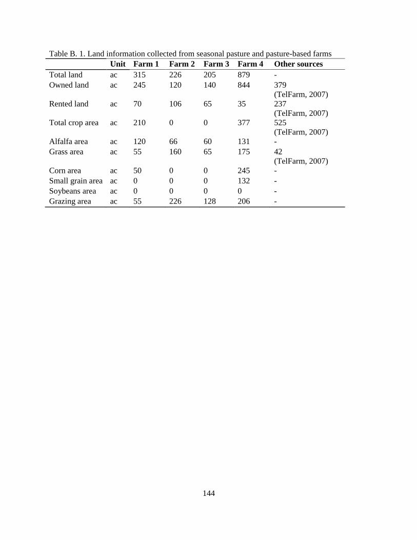
144
Table B. 1. Land information collected from seasonal pasture and pasture-based farms
Unit Farm 1 Farm 2 Farm 3 Farm 4 Other sources
Total land ac 315 226 205 879 -
Owned land ac 245 120 140 844 379
(TelFarm, 2007)
Rented land ac 70 106 65 35 237
(TelFarm, 2007)
Total crop area ac 210 0 0 377 525
(TelFarm, 2007)
Alfalfa area ac 120 66 60 131 -
Grass area ac 55 160 65 175 42
(TelFarm, 2007)
Corn area ac 50 0 0 245 -
Small grain area ac 0 0 0 132 -
Soybeans area ac 0 0 0 0 -
Grazing area ac 55 226 128 206 -

145
Table B. 2. Crop information collected from seasonal pasture and pasture-based farms
Unit Farm 1 Farm 2 Farm 3 Farm 4 Other sources
Alfalfa
Stand life for
alfalfa years 3 5 5 5 -
Manure
applied to
alfalfa
% 10 0 0 34 7 (MSU Extension, 2004)
Grass
Stand life for
grass years - 10 12 10 -
Initial Sward
dry matter of
grass
lb/ac - - - 1447 418 (IFSM Default)
Initial Sward
composition of
grass
%
70%
CS and
30% L
67%
CS and
33% L
70%
CS and
30% L
60%
CS and
40% L
-
Manure
applied to
grass
% 0 100 100 0 -
Corn
Plant
population of
corn
plant/ac 30,000 - - 25,000 25,000-30,000 (IFSM
Default)
Relative
maturity index
of corn
days 95 - - 103 -
Manure
applied to corn % 90 - - 10 3 (MSU Extension, 2004)
[a] CS= Cool-season grass; L=Legume
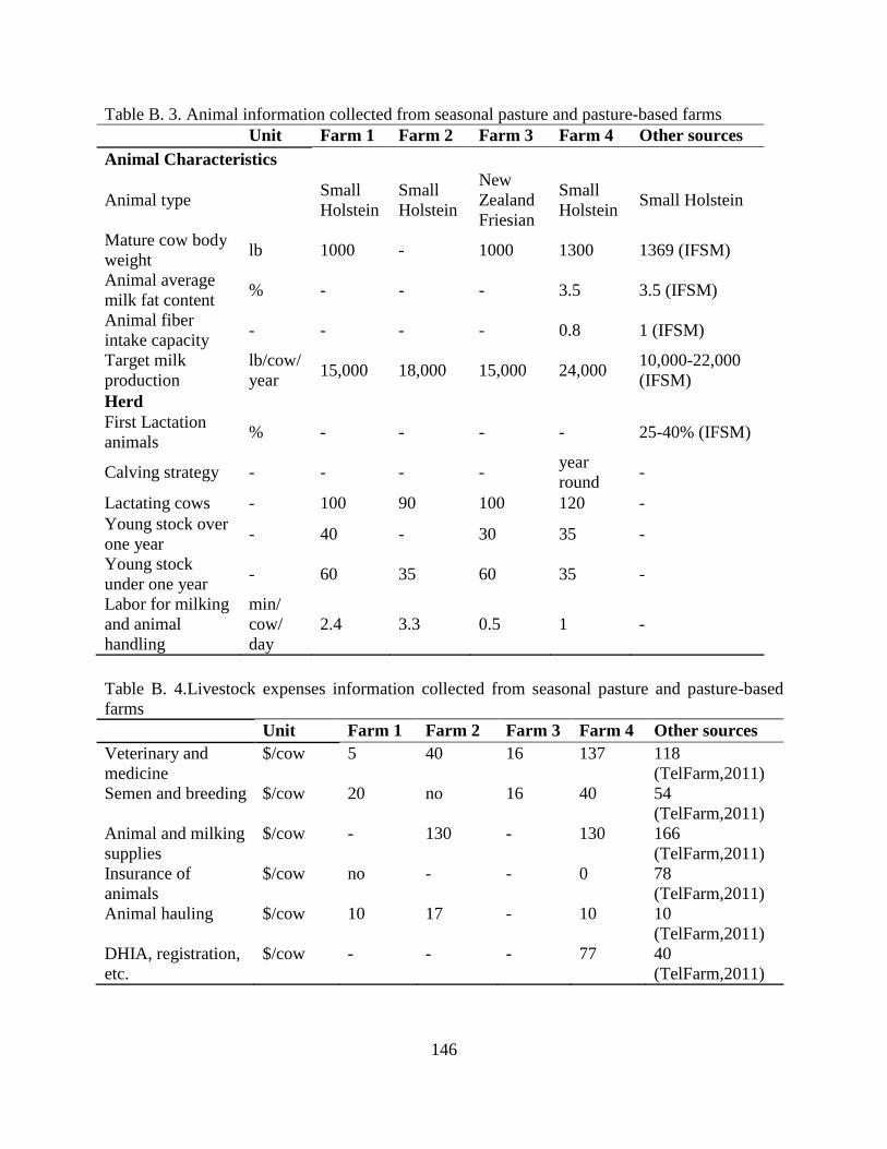
146
Table B. 3. Animal information collected from seasonal pasture and pasture-based farms
Unit Farm 1 Farm 2 Farm 3 Farm 4 Other sources
Animal Characteristics
Animal type
Small
Holstein
Small
Holstein
New
Zealand
Friesian
Small
Holstein Small Holstein
Mature cow body
weight lb 1000 - 1000 1300 1369 (IFSM)
Animal average
milk fat content % - - - 3.5 3.5 (IFSM)
Animal fiber
intake capacity - - - - 0.8 1 (IFSM)
Target milk
production
lb/cow/
year 15,000 18,000 15,000 24,000
10,000-22,000
(IFSM)
Herd
First Lactation
animals % - - - - 25-40% (IFSM)
Calving strategy - - - - year
round -
Lactating cows - 100 90 100 120 -
Young stock over
one year - 40 - 30 35 -
Young stock
under one year - 60 35 60 35 -
Labor for milking
and animal
handling
min/
cow/
day
2.4 3.3 0.5 1 -
Table B. 4.Livestock expenses information collected from seasonal pasture and pasture-based
farms
Unit Farm 1 Farm 2 Farm 3 Farm 4 Other sources
Veterinary and
medicine
$/cow 5 40 16 137 118
(TelFarm,2011)
Semen and breeding $/cow 20 no 16 40 54
(TelFarm,2011)
Animal and milking
supplies
$/cow - 130 - 130 166
(TelFarm,2011)
Insurance of
animals
$/cow no - - 0 78
(TelFarm,2011)
Animal hauling $/cow 10 17 - 10 10
(TelFarm,2011)
DHIA, registration,
etc.
$/cow - - - 77 40
(TelFarm,2011)

147
Table B. 5. Animal feeding information collected from seasonal pasture and pasture-based farms
Unit Farm 1 Farm 2 Farm 3 Farm 4 Other
sources
Feeding method
Grain - Loader
and mixer
wagon
Individual
computer
feeder
Individual
computer
feeder
Loader and
mixer
wagon
-
Silage - No No No Loader and
mixer
wagon
-
Hay - Hand fed Self-fed in
hay feeder
Self-fed in
hay feeder
Self-fed in
hay feeder
-
Ration Constituents
Minimum dry
hay in cow ration
% of
forage
80 - - 0 33
(USDA,
2000)
Phosphorus
feeding level
% of
NRC
recom.
- - - 107 -
Protein feeding
level
% of
NRC
recom.
- - - 109 -
Relative forage
to grain ratio
- High High - High -
Crude protein
supplement
- No No Soybean
meal 48%
Soybean
meal 44%
-
Undegradable
protein
- Roasted
soybean
Distillers
grain
- Distillers
grain
-
Energy
supplement
- Grain Grain Grain Grain -

148
Table B.6. Animal facilities information collected from seasonal pasture and pasture-based farms
Unit Farm 1 Farm 2 Farm 3 Farm 4
Milking center[a]
Type - Double 12
parlor
Pipeline
system
Automatic
Robotic
System,
multi stall
Automatic
Robotic
System,
multi stall
Structure cost $ 60,000 57,000 150,000 600,000
Equipment cost $ 30,000 42,000 310,000 400,000
Cow housing[a]
Type -
Free stall
barn,
naturally
ventilated
Bedded pack
barn
Bedded pack
barn
Free stall
barn,
naturally
ventilated
Structure cost $ 45,000 - - 1,000,000
Heifer housing[a]
Type -
Free stall
barn,
naturally
ventilated
Bedded pack
barn
Calf hutches
and dry lot
Free stall
barn,
naturally
ventilated
Structure cost $ - - 35,000 300,000
Feed facility[a]
Type -
Short term
storage of
premix
Short term
storage of
premix
Short term
storage of
premix
Short term
storage of
premix
Structure cost $ 200 - - 200,000
[a] No information collected from other sources
Table B. 7. Manure information collected from seasonal pasture and pasture-based farms
Unit Farm 1 Farm 2 Farm 3 Farm 4
Other
sources
Manure Characteristics
Type % DM 12-14 12-14 12-14 12-14 -
Dry matter
content % - - - -
10
(ASABE,
2013a)
Nitrogen
content % DM - - - -
3.8
(ASABE,
2013a)
Organic
nitrogen
content
% total
N - - - -
70
(ASABE,
2013a)

149
Phosphorus
content % DM - - - -
0.8
(ASABE,
2013a)
Potassium
content % DM - - - -
2.4
(ASABE,
2013a)
Collection and Use
Collection
method -
Scraper
with
bucket
loading
Scraper
with ramp
loading
Scraper
with
slurry
pump
Scraper
with
bucket
loading
-
Incorporation
by tillage - No No No No -
Average
hauling
distance
mile 2 1 1 9 -
Field
application
method
- Broadcast
spreading
Broadcast
spreading
Broadcast
spreading
Broadcast
spreading -
Manure Storage
Type -
Top-
loaded
concrete
tank
Top-
loaded
concrete
tank
Bottom-
loaded
tank or
basin
Top-
loaded
concrete
tank
Top-
loaded
concrete
tank (MI
Gov.,
2012)
Storage period months None 1 3 6 -
Capacity ton 124 357 309 3000 -
Storage initial
cost $ 4000 15000 - 103000 -
Bedding
Type of
bedding - Sand Straw Saw dust
Chopped
straw -
Amount of
bedding
lb/cow/
day 3 18 0.60 3 -
Import/Export of manure
Import - No No No No -
Export - No No No 25% -
Table B.7 (cont’d)

150
Table B. 8. Storage structures information collected from seasonal pasture and pasture-based
Unit Farm 1 Farm 2 Farm 3 Farm 4
Storage 1[a]
Type of storage - Sealed silo Sealed silo Stave silo Sealed silo
Type of forage or
grain stored
High quality
forage (Dry corn)
Grain for
milk cows
High
moisture
grain
Grain crop silage
(Dry grain)
Quantity - 4 2 1 1
Capacity ton
DM 432 12 203 76
Initial cost $ 7,000 1,100 42,000 -
Storage 2[a]
Type of storage - - Bale - Pressed bag
Type of forage or
grain stored -
hay -
Low and high
quality forage
Capacity ton
DM - 0.3/bale - 70
Initial cost $ - 40/bale - 20
Annual cost $/ ton
DM - 500 - -
Storage 3[a]
Type of storage - - Sealed silo - Bunker silo
Type of forage or
grain stored -
Grain for
calves -
Grain crop silage
(corn and alfalfa)
Quantity -
1 - 1 for corn silage and
3 for alfalfa
Capacity ton
DM - 8 - 270
Initial cost $ - 100 - 55,625
Initial cost $/ton
DM - 12.5 - 206
Storage 4[a]
Type of storage - - - - Inside a shed
Type of forage or
grain stored - - - - Dry hay
Quantity - - - - 1
Capacity ton
DM - - - 300
Initial cost $ - - - 50,000
Initial cost $/ton
DM - - - 167
[a]No information collected from other sources

151
Table B. 9. Economic information collected from seasonal pasture and pasture-based farms
Unit Farm 1 Farm 2 Farm 3 Farm 4 Other sources
General rates
Diesel fuel $/gal - - - - 3.68(U.S Energy, 2013)
Electricity $/KWh - - - - 0.13 (MI Public
Service, 2012)
Grain drying
$/pt/
ton
DM
- - - - 1.6 (MSU custom
machine, 2013)
Labor wage $/h - - - 30 11.3 (MI AEWR, 2013)
Land rental $/acre - - - 70 50.98 (TelFarm, 2011)
Property tax % - - - 0 2.5 (IFSM default)
Fertilizer prices
N $/lb - - - 0.61 0.53 (Purdue Extension,
2011)
P $/lb - - - 1.68 0.56 (Purdue Ext.,2011)
K $/lb - - - 0.59 0.47 (Purdue Ext.,2011)
Lime $/ton
0.01 (Purdue Ext.,2011)
Annual seed and
chemicals
New forage stand $/acre 200 200 200 133 84 (Iowa State
University, 2012)
Established forage
stand $/acre 0 0 0 7 -
Corn land $/acre 200 - - 100 223
(NASS,2010)
Oats land $/acre - - - - -
Soybean land $/acre - - - 58 104.39
(NASS,2010)
Additional for
corn following
corn rotation
$/acre - - - 5
Buying prices
Soybean meal
44%
$/ ton
DM - - - 184 365 (MSU, 2013)
Distillers grain $/ ton
DM - - - - 150 (IFSM, 2012)
Corn grain $/ ton
DM - - 376 - 145(USDA, 2013)
Hay $/ ton
DM - 500 320 - 180 (USDA, 2013)
Fat $/ ton - - 200 184 -
Minerals /
vitamins $/ ton - 2,345 200 184 -

152
Bedding material $/ ton 6 0 170 100 -
Custom
operations No No No No -
Table B. 10. Grazing information collected from seasonal pasture and pasture-based farms
Unit Farm 1 Farm 2 Farm 3 Farm 4 Other sources
Grazing area ac 55 226 128 206 1 ac/cow* (NRCS)
Grazing management costs
Investment in
perimeter fence $ 10,000 12,600 1,600 14,500
$29/ac* (Iowa State
U, 2012)
Investment in
temporary fence $ 2,000 1,400 - 8,000
$17/ac* (Iowa State
U, 2012)
Investment in watering
system $ no 2,500 1,770 15,000 $25/ac* (NRCS)
Added annual cost of
seed and chemical $/ac 54.5 82 135 10 -
Grazing strategy
Labor for grazing
management
h/
week 10 10 10 6 -
Types of animals
grazed - all all all all -
Time on pasture h 22 22 22 22 -
* The cost of perimeter fence is $0.89 /ft and temporary fence is $0.2/ft(Iowa State Extension,
2012). To convert the cost per feet to cost per acre it was assumed each paddock area is 3 ac
(from where is obtained the perimeter of all paddocks). Total number of paddocks were
calculated based equations 1,2 and 3 and data from Table B.11.
*Watering system were calculated with equations 4, 5 and 6, and based on data from Table B.12.
(1)
(2)
Paddocks acres* Number of paddocks (3)
Table B.9 (cont’d)

153
Table B. 11. Data for calculations for fence investments
Data for calculations for fence investments
Recommended by NRCS
(Purdue Extension AY-328)
Data
used
Forage species of cool season grass 70% of Orchadgrass, Tall
fescue, perennial ryegrass
-
Forage species for legume 30 % of white clover -
A: Height of cool season grass to start grazing (in) 6-8 7
Height of legume to start grazing (in) 6-10 7
Rest period for cool season grass (days) 30-45 30
Rest period for legume (days) 24-32 30
Estimated dry matter yield of cool season grass mix
(lb/ac/in)
200-300 250
Daily forage dry matter intake for lactating dairy
cow (%)
3-4 3
Grazing efficiency for 8 paddock system (%) 60% 60
Paddock acres - 3
Animal weight - 1000
Number of animals per paddock - 25
(4)
(5)
(6)
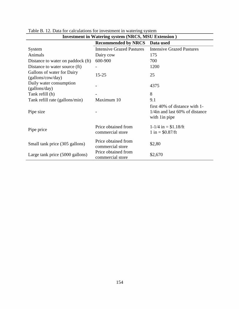
154
Table B. 12. Data for calculations for investment in watering system
Investment in Watering system (NRCS, MSU Extension )
Recommended by NRCS Data used
System Intensive Grazed Pastures Intensive Grazed Pastures
Animals Dairy cow 175
Distance to water on paddock (ft) 600-900 700
Distance to water source (ft) - 1200
Gallons of water for Dairy
(gallons/cow/day) 15-25 25
Daily water consumption
(gallons/day) - 4375
Tank refill (h) - 8
Tank refill rate (gallons/min) Maximum 10 9.1
Pipe size -
first 40% of distance with 1-
1/4in and last 60% of distance
with 1in pipe
Pipe price Price obtained from
commercial store
1-1/4 in = $1.18/ft
1 in = $0.87/ft
Small tank price (305 gallons) Price obtained from
commercial store $2,80
Large tank price (5000 gallons) Price obtained from
commercial store $2,670

155
APPENDIX C: DATA SELECTED FOR THE FIVE REPRESENTATIVE DAIRY
PRODUCTION SYSTEMS

156
Table C. 1. Representative farms
Scenario Characteristics
F1 Confinement
F2 Confinement with AD
F3 Seasonal 140 cows
F4 Seasonal pasture with imported manure, cash crop and AD
F5 Annual pasture-based
F6 Confinement 500 cows
Table C. 2. Land information selected for farms F1, F2, F3, F4, F5, F6
Unit F1 F2 F3 F4 F5 F6
Total land ac 275 275 275 2000 275 1270
Owned land ac 175 175 175 175 175 175
Rented land ac 100 100 100 1825 100 1095
Total crop area ac 275 275 275 1875 0 1270
Alfalfa area ac 90 90 25 25 100 450
Grass area ac 0 0 125 125 175 0
Corn area ac 185 185 125 925 0 820
Soybeans area ac 0 0 0 925 0 0

157
Table C. 3. Crop information for farms F1, F2, F3, F4, F5, F6
[a] The amount of manure applied is the percentage of the amount of manure collected on the
milking center
[b]CS =Cool-Season grass; L=Legume
Unit F1 F2 F3, F4 F5 F6
Alfalfa
Stand life year 4 4 4 4 4
Yield adjustment
factor
% 100 100 100 100 100
N application rate lb/ac 0 0 0 0 0
P application rate lb/ac 0 0 0 0 0
K application rate lb/ac 0 0 0 0 0
Manure applied[a] % 0 0 0 20 0
Corn
Plant population plant/ac 28,000 28,000 28,000 - 28,000
Relative maturity
index
days 100 100 100 - 100
Yield adjustment
factor
% 100 100 100 - 100
N application rate,
pre-planting
lb/ac 0 0 0 - 0
N application rate,
post-planting
lb/ac 25 25 25 - 25
P application rate lb/ac 0 0 0 - 0
K application rate lb/ac 0 0 0 - 0
Manure applied % 100 100 100 - 100
Grass
Stand life years - - 10 10 -
Initial Sward dry
matter
lb/ac - - 418 418 -
Initial Sward
composition of
% - - 70% CS
and 30%
L[b]
70% CS
and 30%
L[b]
-
Yield adjustment
factor
% - - 110 110 -
N application rate lb/ac - - 0 0 -
P application rate lb/ac - - 0 0 -
K application rate lb/ac - - 0 0 0
Manure applied[a] % - - 0 80 0

158
Table C. 4. Grazing information for farms F3, F4 and F5
Unit F3, F4 F5
Grazing area
Spring ac 75 100
Summer ac 125 175
Fall ac 100 150
Grazing management costs
Investment in perimeter fence $ 3,625 5,075
Investment in temporary fence $ 2,125 2,975
Investment in watering system $ 3,125 4,375
Added annual cost of seed and
chemical
$/ac 30 30
Grazing strategy
Labor for grazing management h/week 10 10
Grazed forage yield adjustment
factor
% 120 120
Types of animals grazed - All cows All cows
Time on pasture h Full days during
grazing season
Full days during
grazing season

159
Table C. 5. Animal information for farms F1, F2, F3, F4, F5, F6
[a] Hols = Holstein
Unit F1 F2 F3, F4 F5 F6
Animal Characteristics
Animal type - Large
Hols[a]
Large
Hols
Medium
Hols
Small
Hols
Large
Hols
Mature cow
body weight lb 1600 1600 1300 1000 1600
Animal average
milk fat content % 3.5 3.5 3.8 4.2 3.5
Animal fiber
intake capacity - 1 1 1 1 1
Target milk
production lb/cow/ year 24,000 24,000 20,000 16,000 24,000
Herd
First Lactation
animals % 35 35 25 30 35
Calving strategy - Year
round
Year
round
Year
round
Year
round
Year
round
Lactating cows - 100 100 142 160 500
Young stock
over one year - 38 38 54 61 190
Young stock
under one year - 42 42 60 67 210
Labor for
milking and
handling
min/cow/day 5.25 5.25 3.0 3.0 5.25
Livestock Expenses
Veterinary and
medicine $/cow 118 118 85 101 118
Semen and
breeding $/cow 54 54 39 46 54
Animal and
milking supplies $/cow 166 166 107 143 166
Insurance of
animals $/cow 78 78 78 78 78
Animal hauling $/cow 10 10 10 10 10
DHIA,
registration $/cow 40 40 40 40 40

160
Table C. 6. Animal feeding information for farms F1, F2, F3, F4, F5, F6
Unit F1, F2, F3, F4 F5, F6
Feeding method
Grain - Loader and mixer
wagon
Loader and mixer
wagon
Silage - Loader and mixer
wagon
Loader and mixer
wagon
Hay - Bale grinder Bale grinder
Ration Constituents
Minimum dry hay in cow
ration
%
forage 5 0
P feeding level % NRC recom. 100 100
Protein feeding level % NRC recom. 100 100
Relative forage: grain - High High
Crude protein supplement - Soybean meal
48%
Soybean meal
48%
Undegradable protein - Distiller Grain Distiller Grain
Energy supplement - Grain Grain
Table C. 7. Animal facilities information for farms F1, F2, F3, F4, F5, F6
Unit F1, F2 F3, F4 F5 F6
Milking center
Type - Double 6
parlor
Double 6
parlor
Double 6
parlor
Double 12
parlor
Structure cost $ 182,000 182,000 137,000 274,000
Equipment cost $ 233,600 233,600 175,000 350,000
Cow housing
Type -
Free Stall
Barn,
naturally
ventilated
Free Stall
Barn,
naturally
ventilated
None
Free Stall
Barn,
naturally
ventilated
Structure cost $ 140,000 196,000 - 700,000
Heifer housing
Type -
Calf
hutches
and dry lot
Calf
hutches
and dry lot
Calf
hutches
and dry lot
Calf
hutches
and dry lot
Structure cost $ 26,700 37,450 42,650 133,500
Feed facility
Type -
Short term
storage
premix
Short term
storage
premix
Short term
storage
premix
Short term
storage
premix
Structure cost $ 4,500 6,300 7,200 22,500

161
Table C. 8. Manure information for farms F1, F2, F3, F4, F5, F6
Unit F1 F2 F3, F4 F5 F6
Manure Characteristics
Type % DM 12-14 12-14 12-14 12-14 12-14
Dry matter content % 10 10 10 10 10
Nitrogen content % DM 3.8 3.8 3.8 3.8 3.8
Organic nitrogen content % total N 70 70 70 70 70
Phosphorus content % DM 0.8 0.8 0.8 0.8 0.8
Potassium content % DM 2.4 2.4 2.4 2.4 2.4
Collection and Use
Collection method -
Scraper
with
slurry
pump
Scraper
with
slurry
pump
Scraper
with
slurry
pump
Scraper
with
bucket
loading
Scraper
with
slurry
pump
Incorporation by tillage - Within
2 days
Within
2 days
Within
2 days No
Within
2 days
Average hauling distance mile 0.5 0.5 0.75 0.5 1.0
Manure Storage
Type -
Top-
loaded
lined
earthen
basin
Top-
loaded
lined
earthen
basin
Top-
loaded
lined
earthen
basin
Slab with
buckwall
Top-
loaded
lined
earthen
basin
Storage period months 6 6 6 0 6
Capacity ton 1,882 1,882 1,699 0 9,227
Storage initial cost $ 45,224 45,224 44,322 0 81,223
Bedding
Type of bedding - Chop
Straw
Chop
Straw
Chop
Straw None
Chop
Straw
Amount of bedding lb/cow/
day 3 1 1
[a] 0 3
Import/Export of manure
Import ton 0 0 14,200 0 0
Export ton 0 0 0 0 0
[a]Farm F3 has an amount of bedding of 3 lb/cow/day

162
Table C. 9. Storage structure information for farms F1, F2, F3, F4, F5, F6
Unit F1 F2 F3, F4 F5 F6
Storage 1
Type of
storage - Bunker silo
Bunker
silo
Bunker
silo Bale Bunker silo
Type of
forage or
grain stored
- High quality
forage
High
quality
forage
High
quality
forage
High
quality
forage
High quality
forage
Capacity ton
DM 423 423 202 423 2028
Initial cost $ 56,982 56,982 32,567 56,982 198,470
Annual cost $/ ton
DM 2.0 2.0 2.0 2.0 2.0
Storage 2
Type of
storage - Bunker silo
Bunker
silo
Bunker
silo - Bunker silo
Type of
forage or
grain stored
- Grain crop
silage
Grain
crop
silage
Grain
crop
silage
- Grain crop
silage
Capacity ton
DM 476 476 476 - 2,168
Initial cost $ 61,637 61,637 61,637 - 204,508
Annual cost $/ ton
DM 2.0 2.0 2.0 - 2.0
Storage 3
Type of
storage - Stave silo Stave silo - - Sealed silo
Type of
forage or
grain stored
-
High
moisture
grain
High
moisture
grain
- -
High
moisture
grain
Capacity ton
DM 191 191 - - 979
Initial cost $ 38,910 38,910 - - 90,547
Storage 4
Type of
storage -
Inside a
shed
Inside a
shed
Inside a
shed
Inside a
shed
Inside a
shed
Type of
forage or
grain stored
- Dry hay Dry hay Dry hay Dry hay Dry hay
Capacity ton
DM 120 120 120 120 200
Initial cost $ 25,960 25,960 25,960 25,960 50,000
Annual grain
storage
$/ ton
DM 12 12 12 12 12

163
Table C. 10. Machine information for farms F1, F2, F3 and F4
F1,F2 F3, F4
Operation Number Machine
type/size
Tractor
size
Number Machine
type/size
Tractor
size
Harvest/ Feeding
Mowing 1 Mower
conditioner
14 ft
134 hp 1 Mower
conditioner
9 ft
87 hp
Raking
1 Tandem rake
18 ft
47 hp 1 Single rake
9 ft
47 hp
Baling 1 Small round
baler
108 hp 1 Medium
round baler
108 hp
Bale wrapping 0 0 0 1 Large round
bale wrapper
87 hp
Forage chopping 1 Medium
forage
harvester
134 hp 1 Medium
forage
harvester
134 hp
Grain harvesting 1 Medium corn
combine 8
row
none 2[a]
Medium corn
combine 8
row
none
Feed mixing
1 Large mixer
13 ton
87 hp 1 Large mixer
13 ton
87 hp
Silo filling 1 Forage
blower/
bunker
packing
108 hp 1 Forage
blower/
bunker
packing
108 hp
Tillage / Planting
Manure handling 1 Medium
slurry tank
spreader
134 hp 1 Medium
slurry tank
spreader
134 hp
Plowing
1 Coulter-
chisel plow
12 ft
134 hp 1 Coulter-
chisel plow
12 ft
134 hp
Field cultivation 1 Seedbed
conditioner
19 ft
134 hp 1 Seedbed
conditioner
19 ft
134 hp
Row crop planting 1 Corn planter
8 row
108 hp 1 Corn planter
8 row
108 hp
Drill seeding
1 Grain drill
12 ft
47 hp 1 Grain drill
12 ft
47 hp
Spraying
1 Sprayer 50 ft 87 hp 1 Sprayer 50 ft 87 hp
[a]Farm F3 uses 1 medium corn combine of 8 row.

164
Table C. 11. Machine information for farms F5 and F6
F5 F6
Operation Number Machine
type/size
Tractor
size
Number Machine
type/size
Tractor
size
Harvest/ Feeding
Mowing 1 Disc mower
conditioner
10ft
108 hp 2 SP[a]
mower
conditioner 16ft
none
Raking
1 Tandem rake
18 ft
87 hp 1 0 0
Baling 1 Medium
round baler
108 hp 2 Windrow merger
32ft
134hp
Bale wrapping 1 Large round
bale wrapper
87 hp 1 Medium round
baler
108 hp
Forage chopping 0 0 0 1 Large SP forage
harvester
none
Grain harvesting 0 0 0 1 Medium corn
combine 8 row
none
Feed mixing
1 Large mixer
13 ton
87 hp 2 Large mixer 13
ton
108hp
Silo filling 2 Forage blower/
bunker packing
220hp
Tillage / Planting
Manure handling 1 Small V- tank
spreader
108 hp 2 Large slurry tank
spreader
220 hp
Plowing
1 Coulter-chisel
plow 12 ft
134 hp 1 Coulter-chisel
plow 20ft
220hp
Field cultivation 1 Seedbed
conditioner
15ft
87hp 1 Seedbed
conditioner 19 ft
134 hp
Row crop planting 0 0 0 1 Corn planter 8
row
108 hp
Drill seeding
1 Grain drill 8ft 47 hp 1 Grain drill 16ft 108hp
Spraying
0 0 0 1 Sprayer 50 ft 108hp
[a]SP = self-propelled

165
Table C. 12. Miscellaneous information for farms F1, F2, F3 and F4
F1,F2 F3, F4
Operation Number Machine
type/size
Miles
transport
Number Machine
type/size
Miles
transport
Transport
tractors 3 47 hp - 3 47 hp -
Feed/ Manure
loader 1
Medium
skid-steer
loader
- 1
Medium
skid-steer
loader
-
Round bale
loader 1 87 hp - 1 87 hp -
Manure
pump/
agitator
- 108 hp - - 108 hp -
Auxiliary
manure pump - No - - No -
Initial
machine shed
cost
- $25,000 - $25,000
Custom
operations -
Grain
Harvest - -
Grain
Harvest /
Grain crop
planting
-
Transport of feed
Hay 1 Round bale
wagons 0.5 1
Round bale
wagons 0.5
Hay crop
silage 2 Dump wagons 0.5 2
Round bale
wagons and
wrappers
0.5
Grain crop
silage 2 Dump wagons 0.5 2
Dump
wagons 0.5
[a]
Grain
3 Grain wagons 0.5 3
Grain
wagons 0.5
[a]
[a]Farm F3 uses 0.75 miles of hauling distance for grain crop silage and grain
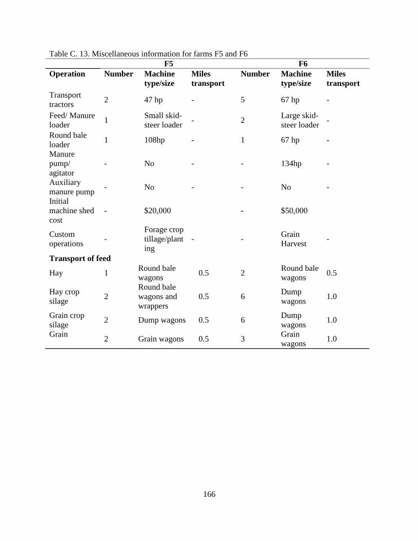
166
Table C. 13. Miscellaneous information for farms F5 and F6
F5 F6
Operation Number Machine
type/size
Miles
transport
Number Machine
type/size
Miles
transport
Transport
tractors 2 47 hp - 5 67 hp -
Feed/ Manure
loader 1
Small skid-
steer loader - 2
Large skid-
steer loader -
Round bale
loader 1 108hp - 1 67 hp -
Manure
pump/
agitator
- No - - 134hp -
Auxiliary
manure pump - No - - No -
Initial
machine shed
cost
- $20,000 - $50,000
Custom
operations -
Forage crop
tillage/plant
ing
- - Grain
Harvest -
Transport of feed
Hay 1 Round bale
wagons 0.5 2
Round bale
wagons 0.5
Hay crop
silage 2
Round bale
wagons and
wrappers
0.5 6 Dump
wagons 1.0
Grain crop
silage 2 Dump wagons 0.5 6
Dump
wagons 1.0
Grain
2 Grain wagons 0.5 3
Grain
wagons 1.0

167
Table C. 14. Tillage and planting information for farms F1, F2, F3, F4, F5, F6
Operation Start date
Alfalfa
Operation 1 Moldboard /Chisel plow 15-Oct
Operation 2 Field cultivator/ conditioner 10-Apr
Operation 3 Field cultivator/ conditioner 10-Apr
Operation 4 Alfalfa seeding 15-Apr
Corn
Operation 1 Moldboard /Chisel plow 10-Sept
Operation 2 Field cultivator/ conditioner 10-Apr
Operation 3 Field cultivator/ conditioner 25-Apr
Operation 4 Corn planting 01-May
Operation 5 Sprayer 10- May
Grass
Operation 1 No operation -
Operation 2 Field cultivator/ conditioner 15-Apr
Operation 3 Field cultivator/ conditioner 20-Apr
Operation 4 Grass seeding 20-Apr
Soybean
Operation 1 Field cultivator/ conditioner 10- Apr
Operation 2 Field cultivator/ conditioner 25- Apr
Operation 3 Soybean planting 01- May
Operation 4 Sprayer 10- May
Max simultaneous operations: 2
Time available for tillage and planting: 8h/day
Table C. 15. Corn harvest information for farms F1, F2, F3, F4, F5, F6
Starting date
Corn Silage 1-Sep
High moisture corn 1-Oct
Dried corn 21-Oct
Harvest detail
Maximum silage moisture content 68%
Corn silage cutting high 6 in
Corn silage processing Rolled with greater chop length
High moisture corn type Grain w/ little or no cob and husk

168
Table C. 16. Alfalfa harvest information for farms F1 and F2
Harvest 1 Harvest 2 Harvest 3 Harvest 4
Drying Treatment
Mechanical
conditioning,
wide swath
Mechanical
conditioning,
wide swath
Mechanical
conditioning,
narrow swath
Mechanical
conditioning,
narrow swath
Tedding treatment No No No No
Raking treatment Before harvest Before harvest Before harvest Before harvest
Harvest type
Wilted silage
harvest by
chopping
Hay harvest by
baling
Wilted silage
harvest by
chopping
Wilted silage
harvest by
chopping
Chemical conditioning
application rate (g/ac) 0 0 0 0
Maximum moisture
content at harvest (%) 68 20 68 68
Critical NDF for high
quality storage (%) 42 42 42 42
Schedule for Alfalfa 4 cuttings- Bud first 2 cuttings, early flower last 2

169
Table C. 17. Alfalfa and grass harvest information for farms F3 and F4, F5
Alfalfa Grass
Harvest 1 Harvest 2 Harvest 3 Harvest 4 Harvest 1
Drying
Treatment
Mechanical
conditioning,
wide swath
Mechanical
conditioning,
wide swath
Mechanical
conditioning,
narrow swath
Mechanical
conditioning,
narrow swath
Mechanical
conditioning,
wide swath
Tedding
treatment No No No No No
Raking treatment Before
harvest
Before
harvest
Before
harvest
Before
harvest
Before
harvest
Harvest type
Round
bailing for
silage
Hay harvest
by baling
Round
bailing for
silage
Round
bailing for
silage
Round
bailing for
silage
Chemical
conditioning
application rate
(g/ac)
0 0 0 0 0
Maximum
moisture content
at harvest (%)
60 20 60 60 60
Critical NDF for
high quality
storage (%)
42 42 42 42 42
Schedule for
Alfalfa
4 cuttings- Bud first 2 cuttings, early flower
last 2
1 cutting-
early head

170
Table C. 18. Alfalfa harvest information for farm F6
Harvest 1 Harvest 2 Harvest 3 Harvest 4
Drying Treatment
Mechanical
conditioning,
wide swath
Mechanical
conditioning,
wide swath
Mechanical
conditioning,
narrow swath
Mechanical
conditioning,
narrow swath
Tedding treatment No No No No
Raking treatment Before harvest Before harvest Before harvest Before harvest
Harvest type
Wilted silage
harvest by
chopping
Wilted silage
harvest by
chopping
Wilted silage
harvest by
chopping
Wilted silage
harvest by
chopping
Chemical conditioning
application rate (g/ac) 0 0 0 0
Maximum moisture
content at harvest (%) 68 65 68 68
Critical NDF for high
quality storage (%) 42 42 42 42
Schedule for Alfalfa 4 cuttings- Bud first 2 cuttings, early flower last 2

171
Table C. 19. Hauling costs for imported manure in seasonal pasture system (F4)
Pumping and trucking from farm to AD
Custom work
Labor hours (h) 301
Custom cost ($/h) 90
Total custom cost ($) 27,090
Hauling from AD to field
Tractor 100 kW
List price ($) 108,000
Purchase price ($) 97,000
Labor hours per tractor (h) 148
Machinery rate ($/h) 25.36
Fuel and lubrication rate ($/h) 26.83
Total tractor cost ($) 15,448
Spreader
List price ($) 44,000
Purchase price ($) 39,600
Machinery rate ($/h) 43.26
Labor hours per spreader (h) 148
Total spreader cost ($) 12,805
Labor
Hours 296
Labor rate ($/h) 16.13
Total labor cost ($) 4,775
Total cost ($) 33,028

172
APPENDIX D: RESULTS FROM IFSM OF THE FIVE REPRESENTATIVE DAIRY
PRODUCTION SYSTEMS

173
Table D. 1. Development of seasonal pasture farm with 142 medium-frame Holsteins, cash crop, imported manure and AD
Unit
Confine [a]
Confine
AD [a]
Confine
AD-
Confine
Seasonal
[b]
Seasonal
AD [b]
Seasonal
AD-
Seasonal
Seasonal
CC/
Import [c]
Seasonal
CC/Import/
AD[d]
Mean Mean % Mean Mean % Mean Mean
Nutrients available, used, and lost to the environment
Nitrogen lost by
leaching lb/ac 12.3 10.9 -11% 45.8 41.7 -9% 11.6 10.3
Nitrogen lost by
denitrification lb/ac 8.7 7.3 -16% 36.2 32.9 -9% 7.2 6.0
Potassium loss
through runoff lb/ac 5.7 5.2 -9% 8.6 8.2 -5% 2.9 2.6
Soil potassium
depletion lb/ac 3 13.1 337% 0 0 0% 0 0.0
Crop removal over
that available on farm % 90 99 10% 76 80 5% 76 80.0
Annual manure production and handling cost
Manure handled ton 17193 16897 -2% 3187 3150 -1% 3179 16897
Manure applied to
corn land ton 17193 16897 -2% 3187 3150 -1% 3179 16897
Machinery cost $ 52790 48297 -9% 18763 16315 -13% 29854 25361
Fuel and electric cost $ 10777 9458 -12% 1771 1543 -13% 8154 6835
Storage cost $ 7081 99463 1305% 3864 19961 417% 3864 96246
Labor cost $ 21004 32078 53% 4115 20162 390% 4775 15849
Annual crop production and feeding costs and the net return over those costs
Equipment cost $ 340664 336864 -1% 95937 95225 -1% 94772.6 92017
Facilities cost $ 243555 335916 38% 84918 101014 19% 85031 177392
Energy cost $ 121078 39560 -67% 20196 7340 -64% 41613 13292
Land rental cost $ 57707 57707 0% 5270 5270 0% 96178 96178
Return to $ 705603 714655 1% 86442 73227 -15% 472633 420348
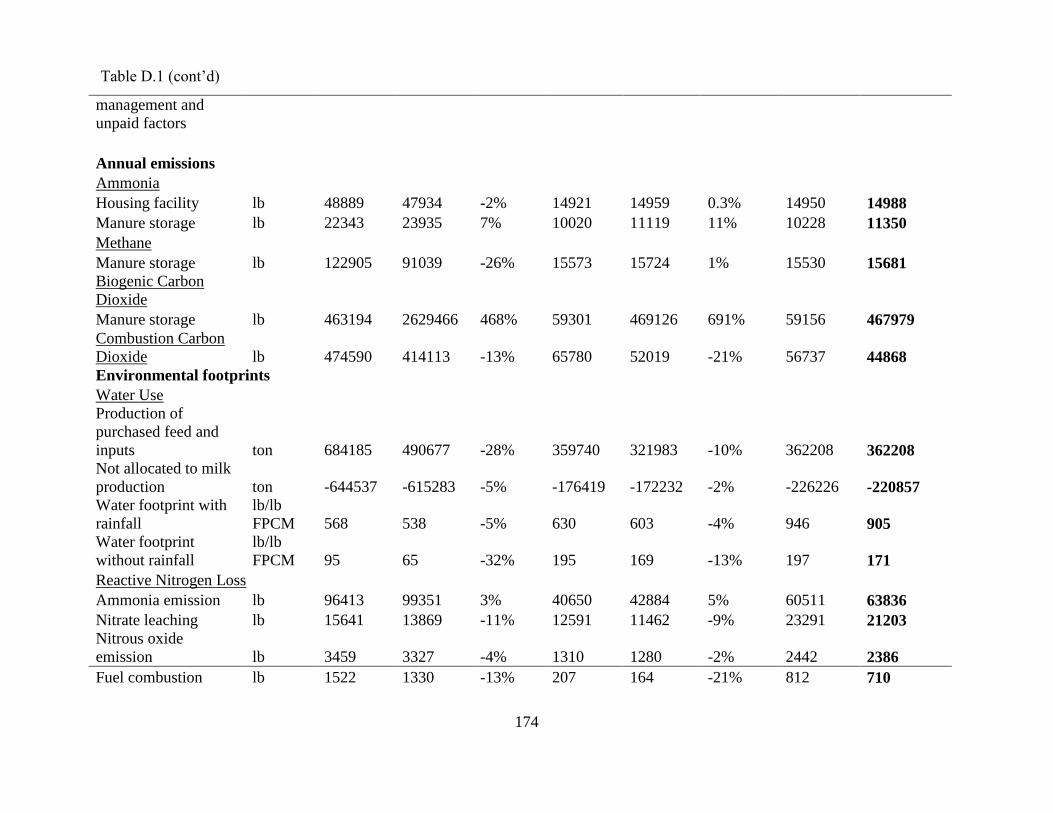
174
management and
unpaid factors
Annual emissions
Ammonia
Housing facility lb 48889 47934 -2% 14921 14959 0.3% 14950 14988
Manure storage lb 22343 23935 7% 10020 11119 11% 10228 11350
Methane
Manure storage lb 122905 91039 -26% 15573 15724 1% 15530 15681
Biogenic Carbon
Dioxide
Manure storage lb 463194 2629466 468% 59301 469126 691% 59156 467979
Combustion Carbon
Dioxide lb 474590 414113 -13% 65780 52019 -21% 56737 44868
Environmental footprints
Water Use
Production of
purchased feed and
inputs ton 684185 490677 -28% 359740 321983 -10% 362208 362208
Not allocated to milk
production ton -644537 -615283 -5% -176419 -172232 -2% -226226 -220857
Water footprint with
rainfall
lb/lb
FPCM 568 538 -5% 630 603 -4% 946 905
Water footprint
without rainfall
lb/lb
FPCM 95 65 -32% 195 169 -13% 197 171
Reactive Nitrogen Loss
Ammonia emission lb 96413 99351 3% 40650 42884 5% 60511 63836
Nitrate leaching lb 15641 13869 -11% 12591 11462 -9% 23291 21203
Nitrous oxide
emission lb 3459 3327 -4% 1310 1280 -2% 2442 2386
Fuel combustion lb 1522 1330 -13% 207 164 -21% 812 710
Table D.1 (cont’d)
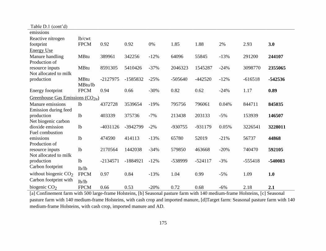
175
emissions
Reactive nitrogen
footprint
lb/cwt
FPCM 0.92 0.92 0% 1.85 1.88 2% 2.93 3.0
Energy Use
Manure handling MBtu 389961 342256 -12% 64096 55845 -13% 291200 244107
Production of
resource inputs MBtu 8591305 5410426 -37% 2046323 1545287 -24% 3098770 2355065
Not allocated to milk
production MBtu -2127975 -1585832 -25% -505640 -442520 -12% -616518 -542536
Energy footprint
MBtu/lb
FPCM 0.94 0.66 -30% 0.82 0.62 -24% 1.17 0.89
Greenhouse Gas Emissions (CO2e)
Manure emissions lb 4372728 3539654 -19% 795756 796061 0.04% 844711 845035
Emission during feed
production lb 403339 375736 -7% 213438 203133 -5% 153939 146507
Net biogenic carbon
dioxide emission lb -4031126 -3942799 -2% -930755 -931179 0.05% 3226541 3228011
Fuel combustion
emissions lb 474590 414113 -13% 65780 52019 -21% 56737 44868
Production of
resource inputs lb 2170564 1442038 -34% 579850 463668 -20% 740470 592105
Not allocated to milk
production lb -2134571 -1884921 -12% -538999 -524117 -3% -555418 -540083
Carbon footprint
without biogenic CO2 lb/lb
FPCM 0.97 0.84 -13% 1.04 0.99 -5% 1.09 1.0
Carbon footprint with
biogenic CO2 lb/lb
FPCM 0.66 0.53 -20% 0.72 0.68 -6% 2.18 2.1
[a] Confinement farm with 500 large-frame Holsteins, [b] Seasonal pasture farm with 140 medium-frame Holsteins, [c] Seasonal
pasture farm with 140 medium-frame Holsteins, with cash crop and imported manure, [d]Target farm: Seasonal pasture farm with 140
medium-frame Holsteins, with cash crop, imported manure and AD.
Table D.1 (cont’d)
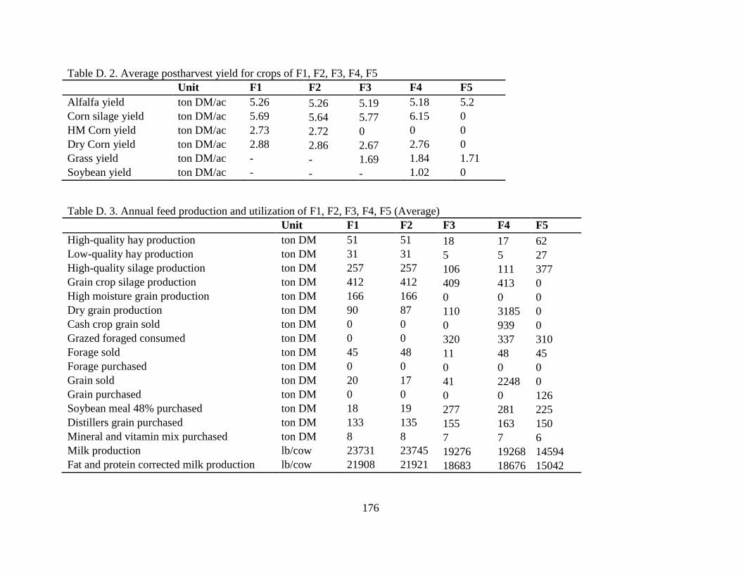
176
Table D. 2. Average postharvest yield for crops of F1, F2, F3, F4, F5
Unit F1 F2 F3 F4 F5
Alfalfa yield ton DM/ac 5.26 5.26 5.19 5.18 5.2
Corn silage yield ton DM/ac 5.69 5.64 5.77 6.15 0
HM Corn yield ton DM/ac 2.73 2.72 0 0 0
Dry Corn yield ton DM/ac 2.88 2.86 2.67 2.76 0
Grass yield ton DM/ac - - 1.69 1.84 1.71
Soybean yield ton DM/ac - - - 1.02 0
Table D. 3. Annual feed production and utilization of F1, F2, F3, F4, F5 (Average)
Unit F1 F2 F3 F4 F5
High-quality hay production ton DM 51 51 18 17 62
Low-quality hay production ton DM 31 31 5 5 27
High-quality silage production ton DM 257 257 106 111 377
Grain crop silage production ton DM 412 412 409 413 0
High moisture grain production ton DM 166 166 0 0 0
Dry grain production ton DM 90 87 110 3185 0
Cash crop grain sold ton DM 0 0 0 939 0
Grazed foraged consumed ton DM 0 0 320 337 310
Forage sold ton DM 45 48 11 48 45
Forage purchased ton DM 0 0 0 0 0
Grain sold ton DM 20 17 41 2248 0
Grain purchased ton DM 0 0 0 0 126
Soybean meal 48% purchased ton DM 18 19 277 281 225
Distillers grain purchased ton DM 133 135 155 163 150
Mineral and vitamin mix purchased ton DM 8 8 7 7 6
Milk production lb/cow 23731 23745 19276 19268 14594
Fat and protein corrected milk production lb/cow 21908 21921 18683 18676 15042

177
Table D. 4. Nutrients available, use and lost to the environment of F1, F2, F3, F4, F5 (Average)
Unit F1 F2 F3 F4 F5
Nitrogen imported to farm lb/ac 174 174 291 189 305.2
Nitrogen exported from farm lb/ac 74.4 74.6 70.5 110 67.5
Nitrogen available on farm lb/ac 266 262 427.1 209 446.4
Nitrogen lost by volatilization lb/ac 68.1 69.9 147.8 31.1 139.9
Nitrogen lost by leaching lb/ac 10.8 9.9 45.8 10.3 17.3
Nitrogen lost by denitrification lb/ac 7.2 6.4 36.2 6.0 10.9
Average nitrogen concentration in leachate ppm 8.8 8.1 37.7 8.1 12.2
N crop removal over that available % 60 61 46 60 46
Phosphorous imported to farm lb/ac 10.5 10.3 20.4 14.2 20
Phosphorous exported from farm lb/ac 12.2 12.2 12.2 14.2 9.9
Phosphorous available on farm lb/ac 17.2 17.2 27.8 15 26.4
Phosphorous loss in runoff and leachate lb/ac 0.3 0.3 0.2 0.5 0
Soil phosphorous build up lb/ac 0 0 8 0 10
Soil phosphorous depletion lb/ac 2.0 2.2 0 0.24 0
P crop removal over that available % 115 117 76 105 64
Potassium imported to farm lb/ac 23.1 13.5 64.6 36.6 46.2
Potassium exported from farm lb/ac 24.6 24.6 18.5 28.1 24.5
Potassium available on farm lb/ac 96.5 86.8 172.4 52.8 174.2
Potassium loss through runoff lb/ac 4.8 4.3 8.6 2.6 8.7
Soil potassium build up lb/ac 0 0 37.4 9.1 13
Soil potassium depletion lb/ac 6.3 15.9 0 0 0
K crop removal over that available % 101 112 76 80 83
Carbon imported to farm lb/ac 6711 6557 5953 9388 7984
Carbon exported from farm lb/ac 998 995 929 1478 789
Carbon loss as carbon dioxide lb/ac 5525 5391 4800 7902 7019
Carbon loss as methane lb/ac 186 169 223 28.1 175
Carbon loss through runoff lb/ac 1.2 1.2 1.2 1.4 0.3

178
Table D. 5. Annual manure production, nutrient availability and handling cost of F1, F2, F3, F4, F5 (Average)
Unit F1 F2 F3 F4 F5
Manure handled ton 3478 3419 3187 16897 2865
Manure applied to alfalfa land ton 0 0 0 0 573
Manure applied to grass land ton 0 0 0 0 2292
Manure applied to corn land ton 3478 3419 3187 16897 0
Manure nitrogen over crop requirement % 51 48 109 58 101
Manure phosphorous over crop requirement % 89 88 136 99 163
Manure potassium over crop requirement % 101 90 135 127 125
Machinery cost $ 16468 14097 18762 25360 8562
Fuel and electric cost $ 1947 1677 1771 6836 1790
Storage cost $ 3943 24062 3864 96246 0
Labor cost $ 4561 20473 4114 15848 5617
Bedding cost $ 8306 2768 8084 2695 0
Total manure handling cost $ 35226 63078 36596 146984 15969
Total cost per mature animal $/cow 352 631 258 1035 100

179
Table D. 6. Annual crop production, feeding costs and net return over those costs of F1, F2, F3, F4, F5 (Average)
Unit F1 F2 F3 F4 F5
Equipment cost $ 85551 87070 80469 164334 45092
Fuel and electric cost $ 9709 9697 6998 17583 6108
Feed and machinery facilities cost $ 21983 21993 15865 15978 10866
Labor cost $ 17867 17839 18379 28084 18702
Seed, fertilizer and chemical cost $ 51111 51112 38949 340373 17128
Grain drying and roasting cost $ 559 522 654 13049 0
Land rental $ 5270 5270 5270 96178 5270
Purchased feed cost $ 38609 39015 130124 129987 128774
Income from feed sales $ 25125 24369 17234 931877 7901
Net feed cost $ 205534 208148 279474 -128050 224037
Net cost per unit of milk $/cwt 8.66 8.77 10.21 - 9.59
Net cost as portion of milk income % 45.6 46.1 53.8 - 50.5
Income from milk sales $ 450900 451160 520062 - 443650
Net return over feed costs $ 245366 243011 240588 - 219613
Net return per cow $/cow 2454 2430 1694 - 1373

180
Table D. 7. Annual production costs and net return to management of F1, F2, F3, F4, F5 (Average)
Unit F1 F2 F3 F4 F5
Equipment cost $ 98926 98090 95937 92017 51273
Facilities cost $ 84452 104581 85262 177623 57599
Energy cost $ 21871 5348 20196 13293 15998
Labor cost $ 73943 89828 64294 81912 71418
Custom operation cost $ 3093 3078 3295 97677 2380
Seed, fertilizer and chemical cost $ 51111 51112 38949 340373 17128
Land rental cost $ 5270 5270 5270 96178 5270
Net purchased feed and bedding cost $ 21791 17414 120973 -799143 120873
Animal purchase and livestock expense $ 46600 46600 50978 50978 66880
Milk hauling and marketing fees $ 23730 23744 27370 27359 23348
Property tax $ 5173 5173 5214 5214 3727
Income from milk sales $ 450900 451160 520062 519862 443650
Income from animal sales $ 61655 61655 83810 83810 80407
Return to management and unpaid factors $ 73594 62578 86133 420192 88162

181
Table D. 8.Crop production costs and feed costs of F1, F2, F3, F4, F5 (Average)
Unit F1 F2 F3 F4 F5
Crop Production costs
Hay $/ton DM 176 178 289 283 126
Hay crop silage $/ton DM 172 173 252 237 135
Grain crop silage $/ton DM 159 160 189 160 0
High-moisture grain $/ton DM 202 203 0 0 0
Dry grain $/ton DM 165 166 204 178 0
Grazed forage $/ton DM 0 0 62.2 59 87
Feed costs
Hay $/ton DM 253 269 339 327 208
Hay crop silage $/ton DM 208 209 283 261 173
Grain crop silage $/ton DM 192 193 223 189 0
High-moisture grain $/ton DM 215 216 0 0 0
Dry grain $/ton DM 166 167 200 187 158
Grazed forage $/ton DM 0 0 80 76 106

182
Table D. 9. Annual emissions of important gaseous compounds of F1, F2, F3, F4, F5 (Average)
Unit F1 F2 F3 F4 F5
Ammonia
Housing facility lb 9493 9288 14918 14986 33370
Manure storage lb 4784 5100 10019 11351 0
Field application lb 8499 9001 15752 42083 5087
Grazing lb 0 0 8729 8822 8313
Total farm lb 22776 23389 49419 77242 46771
Hydrogen Sulfide
Housing facility lb 77 75 65 64 87
Manure storage lb 139 135 110 108 0
Field application lb 502 481 406 2124 0
Grazing lb 0 0 1 1 1
Total farm lb 717 690 582 2297 88
Methane
Housing facility lb 43369 43307 44306 44577 42945
Manure storage lb 24833 18415 15572 15679 0
Field application lb 83 88 157 448 87
Grazing lb 0 0 21885 22075 21229
Total farm lb 68285 61810 81920 82779 64261
Nitrous Oxide
Housing facility lb 450 437 747 825 716
Manure storage lb 324 314 535 592 0
Farmland lb 296 278 776 2244 671
Total farm lb 1070 1030 2058 3661 1387
Biogenic Carbon Dioxide
Housing facility lb 1510026 1509904 1223542 1220864 1110190
Manure storage lb 93567 531874 59298 467938 0
Assimilated in feed lb -2409483 -2830159 -2752647 1618090 -2355195
Grazing animal lb 0 0 538938 538066 480428
Net emission lb -805891 -788382 -930869 3844958 -764576
Combustion Carbon Dioxide lb 78598 66542 65779 44870 53068

183
Table D. 10. Table of environmental footprints of water, nitrogen, energy and carbon for F1, F2, F3, F4, F5 (Average)
Unit F1 F2 F3 F4 F5
Water Use
Feed production, rainfall ton 645706 645876 645670 1111121 644806
Drinking ton 3098 3098 4622 4613 4384
Animal cooling ton 252 252 357 357 403
Parlor and equipment cleaning ton 1006 1006 1428 1428 1609
Production of purchased feed and inputs ton 141444 102164 359683 362089 369910
Not allocated to milk production ton -134981 -129020 -176406 -220842 -159448
Water footprint with rainfall lb/lb FPCM* 600 569 630 905 716
Water footprint without rainfall lb/lb FPCM 99 68 195 170 244
Reactive Nitrogen Loss
Ammonia emission lb 18730 19235 40641 63836 38463
Nitrate leaching lb 2961 2732 12588 21201 4771
Nitrous oxide emission lb 681 656 1310 2386 883
Fuel combustion emissions lb 260 220 207 710 168
Production of resource inputs lb 945 776 2320 2140 2503
Not allocated to milk production lb -4024 -4028 -8133 -11703 -6713
Reactive nitrogen footprint lb/cwt FPCM 0.89 0.89 1.85 3 1.67
Energy Use
Feed production MBtu 204712 204588 133990 181040 109217
Animal feeding MBtu 144480 144035 115955 114529 105202
Manure handling MBtu 70449 60700 64088 244129 64762
Milking and milk cooling MBtu 220185 147002 253959 170087 216645
Animal housing ventilation and lighting MBtu 54782 54782 53622 53622 17147
Production of resource inputs MBtu 1806638 1184093 2046170 2354809 1927342
Not allocated to milk production MBtu -427475 -320825 -505605 -542463 -412267
Energy footprint MBtu/lb FPCM 0.95 0.67 0.82 0.91 0.84

184
Greenhouse Gas Emissions (CO2e)
Animal emissions lb 1061739 1061285 1634396 1646297 1580343
Manure emissions lb 875962 708044 795678 844959 239604
Emission during feed production lb 78141 73297 213429 146502 182560
Net biogenic carbon dioxide emission lb -805891 -788382 -930868 3227514 -764578
Fuel combustion emissions lb 78598 66542 65779 44870 53068
Production of resource inputs lb 455884 313506 579791 592051 613756
Not allocated to milk production lb -427506 -377880 -538952 -540033 -421879
Carbon footprint without biogenic CO2 lb/lb FPCM 0.97 0.84 1.04 1 0.93
Carbon footprint with biogenic CO2 lb/lb FPCM 0.66 0.54 0.72 2.1 0.65
*FPCM is fat and protein corrected milk (4.0% fat and 3.3% protein)
Table D.1 (cont’d)

185
REFERENCES

186
REFERENCES
Acock, B., and Trent, A. (1991). The soybean crop simulator, GLYCIM: documentation for the
modular version 91. Moscow, Idaho: Department of Plant, Soil and Entomological
Sciences, University of Idaho.
ADIAC. (2009). Anaerobic Digestion Initiative Advisory Committee of BC. Retrieved from
Environmental Impacts: http://www.bcfarmbiogas.ca/ad_info/environmental_impacts
Allan, D., Katovich, E., and Nelson, C. (2003). Fertilizer Value and Weed Seed Destruction
Potential of Digested Manure. Anaerobic Digester Technology Applications in Animal
Agric ulture: A National Summit. Raleigh, North : Water Environment Federation.
Archer, D. (1985). Uncoupling of Methanogenic from Growth of Mecthanosarica barkeri by
Phosphate Limitation. Norwich: Applied and Environmental Microbiology: American
Society for Microbiology.
Arora, S. M. (2011). Poultry Manure: The New Frontier for Anaerobic Digestion. S3N
Consulting, LLC.
ASABE. (2013a). American Society of Agricultural Engineers. Retrieved from Manure
production and characteristics:
http://evo31.ae.iastate.edu/ifafs/doc/pdf/ASAE_D384.2.pdf
ASABE. (2013b). American Society of Agricultural Engineers. Retrieved from Agricultural
Machinery Management: http://www3.abe.iastate.edu/ast330/Project/AESE496.3.pdf
ASABE. (2013c). American Society of Agricultural Engineers. Retrieved from Agricultural
Machinery Management Data:
http://www3.abe.iastate.edu/ae340/2006/ASAE_D497.4.pdf
ASABE. (2008). American Society of Agricultural Engineers. Retrieved from Manure
production and characteristics: http://cnmp.unl.edu/D384.2.pdf
Belflower, J. B., Bernard, J. K., Gattie, D. K., Hancock, D. W., Risse, L. M., and Rotz, C. A.
(2012). A case study of the potential environmental impacts of different dairy production
systems in Georgia. Agricultural Systems, 108: 84-93.

187
Benbrook, C., Carman, C., Clark, E. A., Daley, C., Fulwider, W., Hansen, M., et al. (2010). A
Dairy Farm's Footprint: Evaluating the impacts of conventional and organic farming
systems. The organic center.
Betts, C., and Ling, C. (2009). Cooperative Approaches for Implementation of Dairy Manure
Digesters. Washington: USDA: Rural Development.
Binkley, D. F. (2010). The economics of anaerobic digestion under different electricity purchase
agreements. East Lansing: Michigan State University.
Biogas Energy Inc. (2008 ). Biogas Energy Inc. Retrieved September 2012, from Key Elements
of Biogas Energy Anaerobic Digesters: http://www.biogas-
energy.com/site/BiogasEnergy.pdf
Bishop, C. P., and Schumway, C. R. (2009). The Economics of Dairy Anaerobic Digestion with
Coproduct Marketing. Review of Agricultural Economics, 31: 394- 410.
Burke, D. (2001). Washington: Environmental Energy Company. Retrieved from Dairy Waste
Anaerobic Digestion Handbook:
http://makingenergy.com/newsite/publications/Dairy%20Waste%20Handbook%20doc.pd
f
Center for Climate and Energy Solutions. (2011, June). Center for Climate and Energy
Solutions. Retrieved June 2013, from Anaerobic Digesters:
http://www.c2es.org/docUploads/AnaerobicDigesters.pdf
Chen, Y., and Hashimoto, A. (1978). Kinetics of methane fermentation. Biotech and Bioeng,
8:269.
Chen, Y., Yang, G. H., Sweeney, S., and Feng, Y. Z. (2010). Household biogas use in rural
China: A study of opportunities and constraints. Renewable and Sustainable Energy
Reviews, 14: 545- 549.
Chianese , D. S., Rotz , C. A., & Richard, T. L. (2009c). Simulation of methane emissions from
dairy farms to asses greenhouse gas reduction strategies. ASABE, 52(4), 1313-1323.
Chianese, D. S., Rotz, C. A., & Richard, T. L. (2009b). Simulation of nitrous oxide emissions
from dairy farms to assess greenhouse gas reduction strategies. ASABE, 52(4), 1325-
1335.

188
Chianese, D. S., Rotz, C. A., & Richard, T. L. (2009a). Simulation of carbon dioxide emissions
from dairy farms to assess greenhouse gas reduction strategies. ASABE, 52 (4), 1301-
1312.
Chynoweth, D., and Isaacson, R. (1987). Anaerobic Digestion of Biomass. Elsevier Applied
Science, 248-250.
Colorado State University. (undated). Colorado State University. Retrieved from Anaerobic
Digestion at Colorado Cattle Operations:
http://www.engr.colostate.edu/~jlabadie/Decision%20Tree/intro.cfm
Department of Natural Resources and Environment. (2009, January 3). Retrieved from Organic
residuals exemption on farm (Anaerobic Digestion):
http://www.michigan.gov/documents/deq/DEQ-WHMD-On-Farm-Anaerobic-
Digestion_266497_7.pdf
Dupchak, K. (2001). Potassium in dairy cow diets. Retrieved October 28, 2013, from Monitoba
Agriculture, Food and Rural Initiatives:
http://www.gov.mb.ca/agriculture/livestock/nutrition/bza15s00.html
Edwards, W. (2007, September). Department of Economics, Iowa State University. Retrieved
July 3, 2013, from FARMSIM explanation :
http://www2.econ.iastate.edu/classes/econ330/edwards/farmsim/Farmsim_explantion.pdf
El-Mashad, H., and Zhang, R. (2007). Co‐Disgetion of food waste and dairy manure for biogas
production . ASABE, Vol. 50(5): 1815-1821.
EPA. (2012a). Environmental Protection Agency. Retrieved June 5, 2013, from Dairy
Production: http://www.epa.gov/agriculture/ag101/printdairy.html#back
EPA. (2004, February). U.S Environmental Protection Agency. Retrieved from A Manual for
Developing Biogas Systems at Commercial Farms in the United States:
http://nepis.epa.gov/Exe/ZyNET.exe/
EPA. (2005, January Ireland). Environmental Protection Agency. Retrieved from Anaerobic
Digestion: Benefits for Waste Management, Agriculture, Energy, and the Environment:
http://www.epa.ie/downloads/consultation/epa_discussion_paper_anaerobic_digestion.pd
f

189
EPA. (2010). EPA. Retrieved June 10, 2013, from Introduction to the Livestock Analysis Model:
http://www.epa.gov/ruminant.html/library/lam/manual.pdf
EPA. (2011, June 2). United States Environmental Protection Agency. Retrieved June 30, 2013,
from Animal Waste: What's the problem?:
http://www.epa.gov/region9/animalwaste/problem.html
EPA. (2012b). Food Scrap Recycling: A Primer for Understanding Large-Scale Food Scrap
Recycling Technologies for Urban Areas. EPA.
EPA. (2013, May). U.S. Environmental Protection Agency. Retrieved from Operational
Anaerobic Digester Projects at U.S. Dairy Farms: http://www.epa.gov/agstar/projects/
EPA-AgStar. (2004). A Manual For Developing Biogas Systems at Commercial Farms in the
United States. Florida: U.S Environmental Protection agency.
EPA-AgSTAR. (2007). AgSTAR Energy and Pollution Prevention. Retrieved July 20, 2012,
from Anaerobic Digesters Continue Growth in U.S. Livestock Market: 11/2007b.
http://www.epa.gov/agstar/pdf/2007_digester_update.pdf
EPA-AgSTAR. (2010a, October). U.S Environmental Protection Agency. Retrieved from U.S
Anaerobic Digester Status Report:
http://www.epa.gov/agstar/documents/digester_status_report2010.pdf
EPA-AgSTAR. (2010b, May). U.S Environmental Protection Agency. Retrieved from Anaerobic
Digestion Capital Costs for Dairy Farms:
http://www.epa.gov/agstar/documents/digester_cost_fs.pdf
EPA-AgSTAR. (2011a). Protocol for Quantifying and Reporting the Performance of Anaerobic
Digestion Systems for Livestock Manures . Massachusetts: EPA.
EPA-AgSTAR. (2011b). AgSTAR. Retrieved from U.S Anaerobic digester status: A 2011
snapshot: http://www.epa.gov/agstar/documents/2011_digester_update.pdf
EPA-AgSTAR. (2012b, September 27). AgSTAR. Retrieved June 7, 2013, from Permitting
Practices for Co-digestion Anaerobic Digester Systems:
http://www.epa.gov/agstar/tools/permitting.html

190
FAO. (2010). Greenhouse Gas Emissions from the Dairy Sector. A Life Cycle Assessment. Food
and Agriculture Organization of the United Nations.
Gerardi, M. (2003). The Microbiology of Anaerobics Digesters. New York: Wiley InterScience.
Ghafoori, E., and Flynn, P. C. (2007). Optimizing the size of anaerobic digesters. ASABE, 50:
1029- 1036.
Goodrich, P. (2005). The Minnesota Project. Retrieved June 2013, from Anaerobic Digester
Systems for Mid- Sized Dairy Farms:
http://www.mnproject.org/pdf/agstar%20report%20full%20update.pdf
Gourley, C. J., Aarons, S. R., and Powell, J. M. (2011). Nitrogen use efficiency and manure
management practices in contrasting dairy production systems. Agriculture, Ecosystems
and Environment, 147:73-81.
Hadrich, J. C., and Wolf, C. A. (2010). Citizen complaints and environmental regulation of
Michigan livestock operations. Journal of Animal Science, 89:277-286.
Hamilton, S. W., DePeters, E. J., McGarvey, J., McGarvey, J. A., Lathrop, J., & Mitloehner, F.
M. (2010). Greenhouse gas, animal performance, and bacterial population structure
responses to dietary Monensin to dairy cows. Environmental Quality, 39:1-9.
Hoard’s Dairyman. (2012, March 10). Hoard’s Dairyman. Retrieved June 29, 2013, from Fewer
dairy farms left the business:
http://www.hoards.com/sites/default/files/Fewer%20dairy%20farms%20left%20the%20b
usiness.pdf
Hoeksma, P., Mosquera, J., & Melse, R. W. (2012). Monitoring methane and nitrous oxide
reduction by manure treatment. Wageningen UR, The Netherlands: Livestock Research,
Report 627.
IEA Bioenergy. (2006, December 31). biogasmax. Retrieved from Biogas production and
utilisation:
http://www.biogasmax.eu/media/2_biogas_production_utilisation__068966400_1207_19
042007.pdf
Intergovernmental Panel on Climate Change (IPCC) . (2007). IPCC. Retrieved 7 28, 2013, from
Climate change 2007: The physical science basis. Contribution of Working Group I to the

191
Fourth Assessment Report of the Intergovernmental Panel on Climate Change. Chapter 2,
Changes in atmospheric constituents and in radiative forcing:
http://www.ipcc.ch/pdf/assessment-report/ar4/wg1/ar4-wg1-chapter2.pdf
Iowa State University. (2010). i-farmtools. Retrieved June 11, 2013, from Short I-FARM
description: http://i-farmtools.iastate.edu/i-farm/I-FARM_short_description.asp
IPCC. (1995). Intergovermental Panel on Climate Change. Retrieved from Second Assesment
Report: http://www.ipcc.ch/pdf/climate-changes-1995/ipcc-2nd-assessment/2nd-
assessment-en.pdf
IPCC. (2006). Emissions from livestock and manure management.
PCC. (2007). Chapter 2: Changes in atmospheric constituents and in radiative forcing.
Retrieved 11 2013, from Climate Change 2007: The Physical Science Basis. Contribution
of Working Group I to the Fourth Assessment Report of the Intergovernmental Panel on
Climate Change: http://www.ipcc.ch/publications_and_data/ar4/wg1/en/ch2.html
Jarvis, S. C., Lovell, R. D., & Panayides, R. (1995). Patterns of methane emission from excreta
of grazing animals. Soil Biol. Biochem, 27(12):1581 – 1588.
Kirk, D., and Faivor, L. (2011). The impact of dairy housing and manure managment on
anaerobic digestion. East Lansing, Michigan: Michigan State University.
Krich, K., Augenstein, D., Batmale, J., Benemann, J., Rutledge, B., and Salour, D. (2005).
Biomethane from Dairy Waste . California: USDA Rural Development.
Kriegl, T., and McNair, R. (2005). Pastures of plenty: Financial performance of Wisconsin
grazing dairy farms. Madison: University of Wisconsin-Madison.
Lake-Brown, N. (2012). Financial feasibilty of biodigester development in Washington State.
Got Manure? Liverpool: Cornell University- Department of Animal Science.
Lansing, S., Botero, R. B., and Martin, J. F. (2008). Waste treatment a nd biogas quality in small
- scale agricultural digesters. Bioresource Technology, 99: 5881 - 5890.
Lazarus, W. F. (2008). Farm-Based Anaerobic Digesters as an Energy and Odor Control
Technology. USDA.

192
Lazarus, W. F. (2009). The Minnesota Project. Retrieved June 6, 2013, from Economic Analysis
ofthe Jer-Lindy Farms Anaerobic Digester:
http://mnproject.org/pdf/LCMR_Digester_factsheet_economics.pdf
Lazarus, W. F., and Rudstrom, M. (2007). The economics of anaerobic digester operation on a
Minnesota dairy farm. Review of Agricultural Economics, 29:349- 364.
Leggett, J., Graves, R. E., and Lanyon, L. E. (Undated). Anaerobic Digestion: Biogas Production
and Odor Reduction from Manure. Retrieved June 6, 2013, from Agricultural and
Biological Engineering. Penn State Extension:
http://pubs.cas.psu.edu/freepubs/pdfs/g77.pdf
Lindemann, W. C., & Glover, C. R. (2003, May). Nitrogen Fixation by Legumes. Guide A-129.
Retrieved October 28, 2013, from New Mexico State University, Agronomy publications:
http://aces.nmsu.edu/pubs/_a/A129/
Loucks, D. P., and Beek, E. (2005). Modelling Methods for Evaluating Alternatives. In D. P.
Loucks, and E. v. Beek, Water Resources Systems Planning and Management: An
Introduction to Methods, Models and Applications (pp. 59-77). The Netherlands: United
Nations Educational, Scientific and Cultural Organization.
Maria, A. (1997). Introduction to modeling and simulation. Winter Simulation Conference, (pp.
7-13).
Mattocks, R., and Wilson, R. (2005). Latest Trends in Anaerobic Digestion in North America.
Biocycle No.46:30.
MDEQ Rector. (2007, January). Michigan Department of Environmental Quality. Retrieved
from Environmental Regulations Affecting Anaerobic Digesters:
http://www.michigan.gov/documents/mda/AD_Regs_221948_7.pdf
Millen, G. (2008). Small- scale digester boosts farm economics. BioCycle, 49: 46 - 47.
Möller H.B. (2007). Results from batch digestion. Not published.
Möller , K., and Müller , T. (2012). Effects of anaerobic digestion on digestate nutrient
availability and crop growth: A review. Eng. Life Sci., No. 3, 242–257.

193
Moser, M. A. (2011). W. D. Hoard and Sons Company. Retrieved October 2012, from Is a
Digester Right for Your Farm?: http://www.rcmdigester.com/publications/Hoards
Dairyman.pdf
Mott, G. O. (1974). Nutrient recycling in pastures. Forage Fertilization, 323-339.
Muller, L. D., and Holden , L. A. (1994). Intensive Rotazional Grazing. Large Animal
Veterinarian, 27-29.
National Research Council. (2003). National Academy Press, Washington, DC. Retrieved June
2013, from Air Emissions from Animal Feeding Operations: Current Knowledge, Future
Needs: www.national-academies.org.
Nelson, C., and Lamb, J. (2002). Haubenschild Farms Anaerobic Digester. Minnesota: The
Minnesota Project.
Norman, S., and Jianguo, M. (2004). A guideline for CoDigestion of food wastes in Farm-based
Anaerobic Digesters. New York: Fact Sheet FW-2, Cornell University.
Nott, S. B. (2003). Evolution of Dairy Grazing in the 1990's. East Lansing, Michigan:
Department of Agricultural Economics, Michigan State University.
Parton, W. J., Holland, E. A., Del Grosso, S. J., Hartman, M. D., Martin, R. E., Moiser, A. R., et
al. (2001). Generalized model for NOx and N2O emissions from soils. Geophys. Res.,
106 (D15): 17403-17419.
Paul, J. W., & Beauchamp, E. G. (1989). Relationship between volatile fatty acids, total
ammonia and pH in manure slurries. Biol. Wastes, 29: 313-318.
Pennington, J. A., and VanDevender, K. (undated). Nutrient and Fertilizer Value of Dairy
Manure. Akansas: University of Arkansas Cooperative Extension Service.
Pennslyvania State University. (2009). Pennslyvania State University: Biogas. Retrieved from
Biogas and Anaerobic Digestion: http://www.biogas.psu.edu/
Powell, J. M., McCrory, D. F., Jackson-Smith, D. B., and Saam, H. (2005). Manure Collection
and Distribution on Wisconsin Dairy Farms. Journal of Environmental Quality, 34:2036-
2044.

194
Purdue Extension. (undated extension bulletin). Managment-Intensive Grazing in Indiana.
Indiana: USDA NRCS.
Ritchie, J. T., Singh, U., Godwin, D. C., and Bowen, W. T. (1998). Cereal growth, development
and yield. In G. Y. Tsuji, G. Hoogenboom, and P. Thornton, Understanting options for
agricultural production (pp. 79-98). Dordrecht, The Netherlands: Kluwer Academic
Publishers.
Ritchie, J., Singh, U., Godwin, D., and Hunt, L. (undated). A User's Guide to CERES-Maize
V2.10. Alabama: International Fertilizer Development Center.
Rotz, A., Corson, M., Chianese, D., Montes, F., Hafner, S., and Coi, C. (2011a). The Integrated
Farm System Model. Reference Manual Version 3.6.
United States Department of Agriculture.
Rotz, C.A. (2004). Management to reduce nitrogen losses in animal production. J. Anim. Sci.
82(E. Suppl.):E119-E137.
Rotz, C. A., Chianese, D. S., Montes, F., and Hafner, S. (2012). Dairy Gas Emissions Model.
Reference Manual. USDA.
Rotz, C.A., Hafner, S.D (2011b). Whole farm impact of anaerobic digestion and biogas use on a
New York dairy farm. ASABE Annual International Meeting. Paper No. 1111194.
Rotz, C. A., Soder, K. J., Skinner, R. H., Dell, C. J., Kleinman, P. J., Schmidt, J. P., and Bryant,
R. B. (2009). Grazing Can Reduce the Environmental Impact of Dairy Production
Systems. Forage and Grazinglands, doi:10.1094/FG-2009-0916-01-RS.
Schaber, J. (undated). Universität Osnabrück . Retrieved June 10, 2013, from FARMSIM: A
dynamic model for the simulation of yields, nutrient cycling and resource flows on
Philippine small-scale farming systems: http://www.usf.uni-
osnabrueck.de/archive/~jschaber/Farmsim/FARMSIM.html
Scottish Executive Environment and Rural Affairs Department. (2007). Nutrient Value of
Digestate from Farm-Based Biogas. Scotland: ADAS and SAC.
Sendich, E. D. (2008). Modeling and analysis of the biorefinery integrated with the agricultural
landscape. Michigan: Michigan State University.

195
Shaver, R., & Hoffman, P. (2010). Use of straw in dairy cattle diets. Wisconsin: University of
Winsconsin Board of Regents.
Sheffield, R., Barker, J., and Rashash, D. (2008). BAE.NCSU. Retrieved from Solids Separation
of Animal Manure:
http://www.bae.ncsu.edu/programs/extension/manure/technologies/solids.pdf
Simpkins, D. (2005). Anaerobic Digester FAQs. Michigan: Michigan Biomass Energy Program.
Michigan Department of Labor and Economic Growth.
Soder, K. J., and Rotz, C. A. (2001). Economic and environmental impact of four levels of
concentrate supplementation in grazing dairy herds. Journal Dairy Sci, 84:2560–2572.
Stokes, J. R., Rajagopalan, R. M., and Stefanou, S. E. (2008). Investment in a Methane Digester:
An Application of Capital Budgeting and Real Options. Review of Agricultural
Economics, 30: 664- 676.
The Minnesota Project. (2010). Anaerobic Digesters: Farm Oportunities and Pathways.
Minnesota: Minnesota Department of Commerce.
The University of Tasmania. (2013). Dairy Greenhouse gas Abatement Strategy calculator. User
Manual. The Department of Agriculture, Fisheries and Forestry.
Totzke, D. (2009). Tapping the Potential of Codigestion. Biocycle, 50 (6).
Tyrell, H. (2002). Nitrogen flow through livestock production systems: Unmanaged loss to the
environment. USDA–ARS, Penn State Univ. Dairy and Animal Science Seminar
U.S Department of Energy. (2012, May 09). Energy Efficency and Renewable Energy. Retrieved
from Energy basics: Anaerobic Digestion:
http://www.eere.energy.gov/basics/renewable_energy/ anaerobic_digestion.html
U.S. Census Bureau. (2012). U.S.Department of Commerce. Retrieved May 2013, from
Statistical Abstract of the United States: Section 17 Agriculture:
http://www.census.gov/compendia/statab/2012edition.html
UDIM. (2013). United Dairy Industry of Michigan. Retrieved July 5, 2013, from Michigan Dairy
facts:

196
http://www.michigandairynewsbureau.org/index.php?option=com_content&view=article
&id=5&Itemid=7
Ündeğer, Ç. (2008). Bilkent Üniversitesi Bilgisayar Mühendisliği Bölümü. Retrieved June 6,
2013, from Introduction To Modeling and Simulation :
http://www.cs.bilkent.edu.tr/~cagatay/cs503/_M&S_02_Introduction.pdf
University of California. (2010, March 23). University of California Agriculture and Natural
Resources. Retrieved June 10, 2013, from Interactive Tools and Models: ALFALFA 1.4:
http://www.ipm.ucdavis.edu/IPMPROJECT/alfalfa.html
University of New Hampshire . (2009). User's Guide for the DNDC Model (Version 9.3) . New
Hampshire : University of New Hampshire .
USDA. (2003). United States Department of Agriculture. Retrieved from Recommended
methods for manure analysis: http://learningstore.uwex.edu/pdf/A3769.pdf
USDA. (2012, October 29). USDA Agricultural Research Service. Retrieved June 6, 2013, from
Integrated Farm System Model: http://www.ars.usda.gov/main/docs.htm?docid=8519
USDA. (2013, 11 12). Integrated Farm System Model. Retrieved 11 14, 2013, from United
States Department of Agriculture-Agricultural Research Service:
http://www.ars.usda.gov/main/docs.htm?docid=8519
USDA-NASS. (2013, February 20). USDA-NASS. Retrieved May 2013, from Milk production:
http://www.usda.gov/nass/PUBS/TODAYRPT/mkpr0213.pdf
USDA-NRCS. (2007). Profitable Grazing-Based Dairy Systems. USDA.
USDOE. (1996). United States Department of Energy. Retrieved from Deploying Anaerobic
Digesters: Current Status and Future Possibilities:
http://www.nrel.gov/docs/legosti/fy96/20558.pdf
Vanhorn, H. H., Wilkie, A. C., Powers, W. J., and Nordstedt, R. A. (1994). Components of Dairy
Manure Manage ment Systems. Journal of Dairy Science, 77: 2008 -2030.
Walsh, J., Ross, C., Smith, M., Harper, S., and Wilkins, W. (1988). Handbook on Biogas
Utilization. Georgia: Georgia Institute of Technology, Engineering Technoloy Branch.

197
Walsh, M. E., and Becker, D. (1996). BIOCOST: A software program to estimate the cost of
producing Bionergy crops. The Seventh National Bioenergy Conference: Partnerships to
Develop and Apply Biomass Technologies. Nashville, Tennessee: Oak Ridge National
Laboratory.
Warncke, D., Dahl, J., Jacobs, L., & Laboski, C. (2004). Nutrients recommendations for field
crops. East Lansing, Michigan: Michigan State University, Extension Bulletin E2904.
Wattiaux, M. A., and Karg, K. L. (2004). Protein level for alfalfa and corn silage-based diets. II.
Nitrogen balance and manure characteristics. Journal Dairy Science, 87:3492-3502.
Wheatley, A. (1990). Anaerobic Digestion: a Waste Treatment Technology. Elsevier Applied
Science, 93-138.
Whitehead, D. C. (1995). Grassland nitrogen. Wallingford, United Kingdom: CABI.
Wilkie, A. (2005). Anaerobic Digestion: Biology and Benefits. New York: Cornell University
63-72.
Winsten, J. R., Parsons, R. L., and Hanson, G. D. (2000). Differentiated Dairy Grazing Intensity
in the Northeast. Journal of Dairy Science , 83:836-842.
Yadav, S. D., Kumar, B., and Thipse, S. S. (2013, January 9). SAE International. Retrieved June
6, 2013, from Effects of Bio-Gas Fuel Composition on Engine Performance:
http://papers.sae.org/2013-26-0011/
Yamulki, S., Jarvis, S. C., & Owen, P. (1999). Methane emission and uptake from soils as
influenced by excreta deposition from grazing animals. Environmental Quality, 28: 676 –
682.
Zhao, L., Rausch, J. N., and Combs, T. L. (2008). Overview of Odor Control for Manure Storage
Facilities. Agriculture and Natural Resources. The Ohio State University Extension., pp.
AEX-738-08.