Embed Size (px)
Citation preview

Arun Bhakta Shrestha
Resource Manual onFlash Flood Risk Management
Module 2: Non-structural Measures

About ICIMODThe International Centre for Integrated Mountain Development (ICIMOD) is an independent regional knowledge, learning and enabling centre serving the eight regional member countries of the Hindu Kush-Himalayas – Afghanistan , Bangladesh , Bhutan , China , India , Myanmar , Nepal , and Pakistan – and the global mountain community. Founded in 1983, ICIMOD is based in Kathmandu, Nepal, and brings together a partnership of regional member countries, partner institutions, and donors with a commitment for development action to secure a better future for the people and environment of the Hindu Kush-Himalayas. ICIMOD’s activities are supported by its core sponsors: the Governments of Austria, Denmark, Germany, Netherlands, Norway, Switzerland, and its regional member countries, along with programme co-fi nancing donors. The primary objective of the Centre is to promote the development of an economically and environmentally sound mountain ecosystem and to improve the living standards of mountain populations.

i
Resource Manual onFlash Flood Risk Management
Module 2: Non-structural Measures
Arun Bhakta Shrestha
International Centre for Integrated Mountain DevelopmentKathmanduJuly 2008

ii
Copyright © 2008International Centre for Integrated Mountain Development (ICIMOD)All rights reserved
Published byInternational Centre for Integrated Mountain DevelopmentG.P.O. Box 3226Kathmandu, Nepal
ISBN 978 92 9115 095 3 (printed) 978 92 9115 096 0 (electronic)
Production teamA. Beatrice Murray (Senior Editor)Mathew Zalichin (Consultant Editor)Susan Sellars-Shrestha (Consultant Editor)Dharma R. Maharjan (Layout and Design)Asha Kaji Thaku (Editorial Assistance)
Cover photosClockwise from top left: 1) Bagmati River at Chobhar, Kathmandu during the fl ash fl ood of July 2003 – Saraju Baidya, DHM; 2) Flash fl ood vulnerability map – Arun B. Shrestha; 3) Flash fl ood modelling in a mountainous catchment – Arun B. Shrestha; 4) Satellite rainfall estimation based on NOAA data – Mandira Shrestha; 5) Flow measurement in a mountain stream using dilution technique – Arun B. Shrestha; 6) A GLOF early warning station established in the Bhotekoshi basin, Nepal – Arun B. Shrestha
Printed and bound in Nepal byHill Side Press (P.) Ltd. Kathmandu
ReproductionThis publication may be reproduced in whole or in part and in any form for educational or non-profi t purposes without special permission from the copyright holder, provided acknowledgement of the source is made. ICIMOD would appreciate receiving a copy of any publication that uses this publication as a source.
No use of this publication may be made for resale or for any other commercial purpose whatsoever without prior permission in writing from ICIMOD.
NoteThe views and interpretations in this publication are those of the author(s). They are not attributable to ICIMOD and do not imply the expression of any opinion concerning the legal status of any country, territory, city or area of its authorities, or concerning the delimitation of its frontiers or boundaries, or the endorsement of any product.
This publication is available in electronic form at http://books.icimod.org.

iii
ContentsForeword vAbout this Module viAcknowledgements viiAcronyms viiiSome Key Terms ix
Chapter 1: Introduction 1
Chapter 2: General Characteristics of HKH Related to Flash Floods 3 2.1 Climate 3 2.2 Hydrology 5 2.3 Geology 10 2.4 Other Factors 10
Chapter 3: Understanding Flash Flood Hazards 11 3.1 Intense Rainfall Flood 11 3.2 Landslide Dam Outburst Flood 14 3.3 Glacial Lake Outburst Flood 20 3.4 Types of Glacial Lakes 21 3.5 Glacial Lake Outburst Flood in the HKH Region 22
Chapter 4: Flash Flood Risk Assessment 25 4.1 What is Risk? 25 4.2 Major Steps in Flash Flood Risk Assessment 26 4.3 Characterisation of the Risk-prone Area 26 4.4 Hazard Analysis 27 4.5 Hazard Assessment 28 4.6 Vulnerability Assessment 29 4.7 Risk Assessment 31
Chapter 5: Flash Flood Risk Management 33 5.1 Non-structural Measures 34 5.2 Risk Reduction 35 5.3 Mitigation Strategies 41
Chapter 6: Hazard-specifi c Flash Flood Management Measures 47 6.1 Intense Rainfall Flood 47 6.2 Landslide Dam Outburst Flood 63 6.3 Glacial Lake Outburst Flood 74
References 87
Annexes (on CD-ROM in back pocket)Annex 1 : Hazard, Vulnerability, and Risk Analysis Annex 2 : Application of GIS to Flood Hazard MappingAnnex 3 : Guiding Principles for Effective Early WarningAnnex 4 : Runoff Curve NumbersAnnex 5 : Training Manual on Flash Flood Modelling using HEC-GEOHMS and HEC HMSAnnex 6 : Inventory of Glaciers and Glacial Lakes, and Identifi cation of Potentially Dangerous Glacial
Lakes

v
ForewordThe Hindu Kush-Himalayan (HKH) region is one of the most dramatic physiographic features on our planet. As the youngest mountain system in the world, it has unstable geological conditions and steep topography, which, combined with frequent extreme weather conditions, makes the region prone to many different natural hazards from landslides, avalanches, and earthquakes, to massive snowfall and fl ooding. Among these, fl ash fl oods are particularly challenging for communities.
Flash fl oods are severe fl ood events that occur with little or no warning. They can be triggered by intense rainfall (‘cloudbursts’), failure of natural or artifi cial dams, and outbursts of glacial lakes. The frequent occurrence of fl ash fl oods within the Hindu Kush-Himalayan region poses a severe threat to lives, livelihoods, and infrastructure, both within the mountains and downstream. Vulnerable groups – the poor, women, children, and people with disabilities – are often the hardest hit. Flash fl oods pose a greater risk to human life and livelihoods than do the more regular riverine fl oods, which build up over days when there is heavy rainfall upstream. Flash fl oods tend to carry with them much higher amounts of debris and, as a result, cause more damage to hydropower stations, roads, bridges, buildings, and other infrastructure.
Since its establishment in 1983, ICIMOD has explored different ways to reduce the risk of disaster from natural hazards and the physical and social vulnerability of the people in the region. These have included training courses, hazard mapping, vulnerability assessments, fostering dialogue among stakeholders, and developing materials for capacity building. Recognising the important role of fl ash fl oods, ICIMOD has recently undertaken several initiatives specifi cally aimed at reducing fl ash fl ood risk. An ‘International Workshop on Flash Floods’ organised by ICIMOD in October 2005 in Lhasa highlighted the need for capacity building in this area. Since then, ICIMOD has been working towards improving the capacity of practitioners and communities to manage fl ash fl ood risk.
Resource materials related to fl ash fl ood risk management have been compiled and developed by ICIMOD together with various partners to support the capacity development and training of planners and practitioners. After testing with different groups, these resource materials are now being published to make them more widely available. The present publication is the second module of a ‘Resource Manual on Flash Flood Risk Management’ and looks at technology-based, non-structural measures for managing fl ash fl oods. It was produced under the project ‘Capacity Building for Flash Flood Risk Management and Sustainable Development in the Himalayas’, funded by the United States Agency for International Development, Offi ce for Foreign Disaster Assistance (USAID/OFDA). The fi rst module focuses on community-based approaches to managing fl ash fl oods. These two modules are small, but important steps towards securing the physical security of the people of the Hindu Kush-Himalayas. We hope that they will contribute towards reducing disaster risk in this vulnerable region.
Andreas Schild Director General ICIMOD

vi
About this ModuleFlash fl oods are among the most destructive natural disasters in the Hindu Kush-Himalayan region. They are sudden events that allow very little time to react. They often occur in isolated remote mountain catchments, where there are few, if any, institutions equipped to deal with disaster mitigation and where relief agencies are either absent or have limited presence and capacity to manage the results of natural disasters. Often the management of fl ash fl oods is done primarily by community-based organisations, local non-governmental organisations, or district and ward-level staff of governmental organisations. However, these people often lack adequate understanding of the processes causing fl ash fl oods and knowledge of fl ash fl ood risk management measures. Building the capacity of those working directly in fl ash fl ood-prone catchments will help to reduce fl ash fl ood risk in the region.
This manual provides resource materials for understanding the problem and managing the risk. The manual is prepared in two modules. The fi rst concerns community-based fl ash fl ood risk management. This second module concerns technology-based non-structural fl ash fl ood risk management. Chapters 1 and 2 of this module introduce the natural setting of the region: topography, geology, climatic systems, and so on. Chapter 3 describes three major types of fl ash fl ood that occur in the region: intense rainfall fl oods, landslide dam outburst fl oods, and glacial lake outburst fl oods, supplemented by examples and case studies. Chapter 4 explains ways to assess fl ash fl ood risks. Chapter 5 describes general, non-structural fl ash fl ood risk management measures. Chapter 6 provides insight into some hazard-specifi c measures.
This module is designed for professionals from both social science and physical science backgrounds. Its objective is to build the capacity of district-level disaster mitigation and relief workers, professionals from community-based and non-governmental organisations such as hydrologists, meteorologists, engineers, and so on. The tools and models selected here are simple, but important, requiring relatively little data. Users with higher technical skills can also benefi t from these tools as a fi rst approach and use higher-level models to further enhance their analysis.
Note: Remote sensing images of the Himalayan region use ESRI as the map source with data from ICIMOD. The Hindu Kush-Himalayan outline shows an approximate boundary based on an ICIMOD working defi nition of mountain/hill areas linked to the mountain ranges that stretch from the Hindu Kush to the Himalayas.

vii
AcknowledgementsThis book is an outcome of the ICIMOD project ‘Capacity Building for Flash Flood Risk Management and Sustainable Development in the Himalayas’, supported by the United States Agency for International Development, Offi ce for Foreign Disaster Assistance (USAID/OFDA).
We are grateful to several colleagues who have contributed to the manual. Muhibuddin Usamah, Asian Disaster Preparedness Center, provided materials on fl ood hazard mapping. GIS-IDC assisted in preparing the manual on using the HEC HMS model for fl ash fl ood modelling. Pradeep Mool and Samjwal Bajracharya provided the manual on spatial data input, attribute data handling, and image processing of Rolwaling Valley, Nepal; and data necessary to use the manual. Pradeep Mool and Samjwal Bajracharya also provided inputs to the section on glacial lake outburst fl oods. Keshar Man Sthapit provided important contributions to the section on watershed management. Professor C.J. van Westen provided the exercise and data on hazard, vulnerability, and risk analysis. We would also like to acknowledge the United Nations International Decade for Natural Disaster Reduction (IDNDR*) for providing the content of Annex 3, Guiding Principles for Effective Early Warning.
Our sincere thanks go to the former Manager of the ICIMOD Water and Hazard Management Programme, Dr. Xu Jianchu, for supporting the initiation of the project and development of this manual, and to the present Manager of the Integrated Water and Hazard Management Programme, Dr. Mats Eriksson, for seeing through the completion of this manual.
Dr. Narendra Khanal, Department of Geography; Dr. Megh Raj Dhital, Central Department of Geology; and Mr. Rupak Rajbhandari, Department of Meteorology of Tribhuvan University provided valuable contributions. Critical comments and constructive suggestions by two external reviewers helped improve the manuscript substantially. Ms. Ezee G.C. provided valuable assistance in preparing the manual.
Many others also contributed to this manual and have generously given permission to reproduce photographs, diagrams, instructions, maps, exercises, and other material; ICIMOD would like to thank them all.
My heartfelt thanks go to many colleagues within and outside ICIMOD, who read the manuscript and provided valuable comments and suggestions.
Thanks also go to the editorial team, A. Beatrice Murray (ICIMOD), Matthew Zalichin (consultant editor), and Susan Sellars-Shrestha (consultant editor/proofreader) for their helpful insights. Heartfelt thanks to the Dharma Ratna Maharjan for his hard work in laying out the manuscript in a very short time and Asha Kaji Thaku for editorial assistance.
* IDNDR (1997) Guiding Principles for Effective Early Warning. Geneva: United Nations International Decade for Natural Disaster Reduction (IDNDR)

viii
AcronymsADPC Asian Disaster Preparedness Center CRU Climate Research UnitDHM Department of Hydrology and Meteorology (Nepal)DPTC Disaster Prevention Technical Centre (Nepal)DWIDP Department of Water Induced Disaster Prevention (Nepal)ESRI Environmental Systems Research InstituteEWS early warning systemFHM fl ood hazard mappingGIS geographical information systemGIS-IDC Geographical Information System Integrated Development CentreGLOF glacial lake outburst fl oodHEC Hydraulic Engineering Center (USA)HF high frequencyHKH Hindu Kush-Himalayas/nHMS Hydrologic Modelling System (HEC)ICIMOD International Centre for Integrated Mountain DevelopmentIDNDR International Decade for Natural Disaster Reduction (UN)IFFM integrated fl ash fl ood managementILWIS The Integrated Land and Water Information System (ITC)ISDR International Strategy for Disaster Reduction (UN)ITC International Institute for Geo-Information Science and Earth Observation (The Netherlands)ITCZ Inter-tropical Convergence ZoneIWRM integrated water resource managementLDOF landslide dam outburst fl oodmasl metres above sea levelMWRS monitoring warning and response systemOFDA Offi ce for Foreign Disaster Assistance (USAID)RGSL Reynolds Geoscience Limited (UK)SCS Soil Conservation Service (now Natural Resources Conservation Service, USA)TU Tribhuvan University (Nepal)UN United NationsUSACE United States Army Corps of Engineers (USA)USAID United States Agency for International DevelopmentUSGS United States Geological SurveyVHF very high frequencyWECS Water and Energy Commission Secretariat (Nepal)WWF World Wildlife Fund/Worldwide Fund for Nature

ix
Some Key TermsThe defi nitions provided here are based on the UN/ISDR Glossary1, UNDP/BCPR (2004), ISDR (2004), and UNU-EHS (2006).
Climate, fl ood and related termsWeather and climate: Weather is a term that encompasses phenomena in the earth’s atmosphere, usually referring to the activity of these phenomena over short periods such as hours or days. Average atmospheric conditions over signifi cantly longer periods of time are known as climate.
Precipitation: Precipitation is the discharge of water, in a liquid or solid state, from the atmosphere, generally upon a land or water surface. Rainfall is precipitation occurring in a liquid state.
Discharge: The volume of water per unit of time that passes through a specifi ed section of a channel is called discharge and is commonly denoted by the letter Q. Discharge can be measured in cubic metres per second (m3/s), sometimes referred to as cumecs. In the English system discharge is measured in ft3/sec or cusec. A cusec is 35.29 times smaller than a cumec.
Flood: Signifi cant rise of water level in a stream, lake, reservoir, or coastal region.
Flash fl ood: Flash fl oods are severe fl ood events triggered by extreme cloudbursts; glacial lake outbursts; or the failure of artifi cial dams or dams caused by landslides, debris, ice, or snow. Flash fl oods can have impacts hundreds of kilometres downstream, although the warning time available is counted in minutes or, at the most, hours.
Annual fl ood: The highest instantaneous peak discharge in a stream that occurs within a hydrological year is called annual fl ood.
Design fl ood: Design fl oods are hypothetical fl oods used for planning and management. As a design fl ood is defi ned by its probability of occurrence, it represents a fl ood that has a particular probability of occurring in any one year. For example, the 1% annual excedence probability (AEP) or 1 in 100 average recurrence interval (ARI) fl ood is a best estimate of a fl ood which has 1 chance in 100 of occurring in any given year.
Flood magnitude: The size of fl ood peak in discharge units (e.g., m3/s, ft3/s, etc.).
Inundation: The state of being submerged under water due to fl ood is called inundation. The depth of water at a particular location is called inundation depth, and the area under submergence is called area of inundation.
Return period: Return period, also known as recurrence interval, is the average interval of time within which the given fl ood will be equalled or exceeded once. For example, a fl ood of 10 years return period is likely to occur on average once in every ten years.
Hazard, risk and related termsHazard2: A potentially damaging physical event, phenomenon, or human activity that may cause the loss of life or injury, property damage, social and economic disruption, or environmental degradation. Hazards can include latent conditions that may represent future threats and can have different origins: natural (geological, hydro-meteorological, biological) or human-induced (environmental degradation and technological hazards).
1 http://www.unisdr.org/eng/library/lib-terminology-eng.htm (Accessed June 2007)2 See Chapter 4 for a detailed description of hazard, vulnerability, and risk.

x
Hazards can be single, sequential, or combined in their origin and effects. Each hazard is characterised by its location, intensity, frequency, and probability.
Vulnerability2: The capacity (or lack of capacity) of a society to anticipate, cope with, resist, and recover from the impact of a natural hazard. A society’s vulnerability is determined by a combination of factors that determine the degree to which life, property, infrastructure, and services are put at risk by a discrete and identifi able event.
Risk2: The chance of loss of life or property, or of injury, damage, or disruption to economic activity due to a particular event for a given area and reference period. Risk is the combination of hazard and vulnerability. Acceptable risk: The level of loss a society or community considers acceptable given existing social, economic, political, cultural, technical, and environmental conditions.
Mitigation: Sustained actions taken to reduce or eliminate a long-term risk to people, infrastructure, and property from hazards and their effects; measures taken in advance of disaster to decrease or eliminate its impact on society and the environment.
Preparedness: Activities to ensure that people are ready for a disaster and respond to it effectively. Preparedness requires deciding what will be done if essential services break down, developing a plan for contingencies, and practising the plan.
Prevention: Activities designed to provide permanent protection from disasters. These include engineering and other physical protective measures, and also non-structural measures (like legislation, incentives, awareness raising, information dissemination) controlling land use, and urban planning.
Recovery: Reconstruction activities carried out after a disaster. They include rebuilding homes, businesses, and public facilities; clearing debris; repairing roads, bridges, and other important infrastructure; and rebuilding sewers and other vital services.
Coping and adaptation strategies: Short- and long-term strategies developed by communities to avoid, minimise, accommodate and/or spread the negative impacts of natural hazards on livelihoods, property and infrastructure, and life.
Structural measures: Action to reduce the effects of fl oods by physical interventions (like retention basins, embankments, dredging, diversions, dams, levees, fl oodwalls, elevating buildings, fl ood-proofi ng).
Non-structural measures: Action to reduce the effects of fl oods using non-physical solutions (like land use planning, fl oodplain zoning, forecasting, advance warning systems, fl ood insurance).
2 See Chapter 4 for a detailed description of hazard, vulnerability, and risk.

1Chapter 1: Introduction
Chapter 1Introduction
The Hindu Kush-Himalayas (HKH) are the youngest mountains on earth and are still tectonically active. They are undergoing uplift and, therefore, the region is characterised by steep slopes and a high rate of surface erosion. In addition to the geological conditions, intense seasonal precipitation in the central and eastern Himalayas, particularly during the summer monsoon, and in the western Himalayas and the Hindu Kush during winter, triggers various types of natural hazards. Floods are one of the most common forms of natural disaster in this region. Intense monsoon rainfall or cloudbursts can cause devastating fl ash fl oods in the middle mountains (500–3500 masl). Rapid melting of snow accumulated during winter is the main cause of fl ash fl oods in the Hindu Kush and western Himalayas. Furthermore, the region is experiencing widespread deglaciation, most probably as a result of global climate change (WWF 2005; Mool et al., 2001; Xu et al. 2007). Deglaciation has caused the birth and rapid growth of many glacial lakes in the region. These lakes are retained by unstable natural moraine dams that tend to break due to internal instabilities or external triggers leading to a glacial lake outburst fl ood (GLOF) that can cause immense fl ooding downstream. Landslides due to intense rainfall in combination with geological instabilities can cause ephemeral damming of rivers. Another type of fl ash fl ood common in the region results from the outbreak of dammed lakes. These dammed lakes can break resulting in fl ash fl ood.
Hundreds of lives and billions of dollars worth of property and investment in high-cost infrastructure are lost in the region every year due to landslides, debris fl ows, and fl oods, along with the destruction of scarce agricultural lands. In the last decade of the 20th Century, fl oods killed about 100,000 persons and affected about 1.4 billion people worldwide. And the number of events as well as deaths are increasing (Figure 1 and Jonkman 2005). Statistics show that the number of people killed per event on average is signifi cantly higher in Asia than elsewhere, and among all water-induced disasters this number is much higher for fl ash fl oods (Jonkman 2005). In Nepal, landslides, fl oods, and avalanches destroy important infrastructure worth US $9 million and cause about 300 deaths annually (DWIDP 2005). In Afghanistan, 362 people were killed or reported missing and 192 people were injured as a direct consequence of fl ash fl oods in 2005 (Azizi and Naimi 2005, cited in Xu et al. 2006). In total, about 100,000 people were displaced by these events. Exceptional events can exceed these numbers by many times — in 1998 the Yangtze fl ood in China caused an estimated US $31 billion of damage (Kron 2005).
Despite the destructive nature and immense impact they have on the socioeconomy of the region, fl ash fl oods have not received adequate attention. This is mainly because of poor understanding of the processes of fl ash fl oods and lack of knowledge of measures to manage the problem in the HKH region.

Resource Manual on Flash Flood Risk Management – Module 22
Figure 1: People killed and affected by fl oods: a. types of water-related disasters; b. number of people killed and affected by fl oods disaggregated by continent; c. number of people killed disaggregated by type of fl ood
0
50
100
150
200
0
500
1000
1500
2000
2500
3000
3500
4000
Africa Americas Asia Europe Oceania
Killed Affected (thousand)
Pe
rso
ns k
ille
d Affe
cte
d (th
ou
sa
nd)
Flood
Landslide/avalanche
Famine
Water rel. epidemic
Drought
0
50
100
150
200
0
0.5
1
1.5
2
2.5
3
3.5
4
Riverine Flood Flash Flood Other
Killed Mortality (%)
Pe
rsons k
illed M
orta
lity (%
)
a.
b.
c.
Sou
rces
: Bas
ed o
n da
ta d
raw
n fr
om J
onkm
an 2
00
5; I
CIM
OD
20
07

3Chapter 2: General Characteristics of HKH Related to Flash Floods
Chapter 2General Characteristics of
HKH Related to Flash FloodsThis chapter provides a brief review of the natural features of the region relevant to fl ash fl oods.
2.1 Climate3
Due to its massive and high mountain systems, the HKH region acts as a barrier to atmospheric circulation, both the summer monsoon and the winter westerlies. The region’s climate, although dominated by the monsoon system, can be characterised by a number of meso- and micro-climates due to topographic variations. The climate in the Himalayas, as in the other parts of South Asia, is dominated by the monsoon system. The summer monsoon originates in the Bay of Bengal and, therefore, the amount of monsoon precipitation decreases from east to west (Figure 2a). The summer monsoon is much longer in the eastern Himalayas (e.g., Assam), where it lasts for fi ve months (June-October); it lasts for four months (June-September) in the central Himalayas (Sikkim, Nepal, and Kumaon), and two months (July-August) in the western Himalayas (e.g., Kashmir) (Chalise and Khanal 2001). The summer monsoon loses its dominance over annual precipitation in the western Himalayas (Figure 3a), where the winter westerlies deliver a signifi cant amount of precipitation (Figure 3b). Winter precipitation is greater in the western parts of the region and less in the eastern parts. The summer monsoon has a meridional pattern as well: precipitation is higher on the windward side of the Himalayas due to the orographic effect on the monsoon air masses, while the leeward side receives less rain. Consequently the Trans-Himalayan zone and the Tibetan plateau receive very little summer precipitation. In the Tibetan Plateau summer monsoon precipitation occurs between May and September (Mei’e et al. 1985). Annual precipitation decreases from southeast to northwest: from about 800 mm at Markam and Songpan in western Sichuan to 400-500 mm at Lhasa, 200-300 mm at Tingri, and less than 100 mm at Ngari Prefecture (Mei’e et al. 1985). Depending on the location, the annual precipitation variation can be quite high (Figure 4). However, in general, the summer monsoon is the predominant source of precipitation in the region (Figures 3, 4).
Temperatures in the Himalayas vary inversely with elevation at a rate of about 0.6°C per 100m, and due to the rugged terrain, wide ranges of temperatures are found over short distances. Local temperatures also correspond to season, aspect, and slope (Zurick et al. 2006). Owing to the thin atmosphere above the Tibetan Plateau and ample and intense radiation, the surface temperature has a large diurnal variation, although its annual temperature range is relatively small. The temperature range in the northern mountainous region of Pakistan and Afghanistan is greater and the annual range of temperature is also quite large. In Chitral (1450 masl), for example, temperatures can reach as high as 42°C and as low as -14.8°C (Shamshad 1988).
High-intensity rainfall is a characteristic microclimatic feature of the region (Domroes 1979). Such high-intensity rainfalls have important implications for fl ash fl oods known as intense rainfall fl oods (IRFs). In July of 1993, 540 mm of rainfall was recorded in 24 hours in the central part of Nepal (Dhital et al. 1993). This caused a devastating fl ash fl ood with colossal damage to infrastructure and lives, and disrupted normal life for several months. These types of events are rather common in the HKH.
The western Himalayas and the Hindu Kush can receive large amounts of snow during the winter, caused by westerly disturbances from the Mediterranean. The snow not only affects peoples’ livelihoods with avalanches and blocked transport routes, but, in case of rapid warming in spring, can also lead to fl ash fl oods caused by rapid snowmelt.
3 With contributions from Mr. R. Rajbhandari, Tri Chandra Campus, Tribhuvan University.

Resource Manual on Flash Flood Risk Management – Module 24
m
<0.4
0.4 - 0.8
0.8 - 1.2
1.2 - 1.6
1.6 - 2.0
2.0 - 2.4
2.4 - 2.8
2.6 - 3.2
3.2 - 3.6
3.6 - 4.0
m
< 10
10 - 25
25 - 50
50 - 75
75 - 100
100 - 125
125 - 150
150 - 175
175 - 200
200 - 225
m
<.5
.5-1
1-1.5
1.5-2
2-2.5
2.5-3
3-3.5
3.5-4
4-4.5
4.5-5
a.
b.
c.
Figure 2: Precipitation distribution in the HKH region: a. during the summer monsoon; b. winter; and c. annual. The blue outline shows the approximate boundary of the region
Sou
rce:
CR
U d
ata;
New
et
al. 2
00
2

5Chapter 2: General Characteristics of HKH Related to Flash Floods
%
< 5
5 - 15
15 - 25
25 - 35
35 - 45
45 - 55
55 - 65
65 - 80
80 - 85
85 - 95
%
< 5
5 - 10
10 - 15
15 - 20
20 - 25
25 - 35
35 - 40
40- 55
55 - 60
60 - 65
a.
b.
Figure 3: Fraction of annual precipitation contributed by: a. summer monsoon and b. winter precipitation. The outline shows the approximate boundary of the region
2.2 HydrologyThe Himalayan range is an important source of runoff, which is signifi cantly higher in the summer than in the winter (Figure 5). The runoff generated in these areas sustains the fl ow of eight4 major rivers that originate from the HKH region (Figure 6). Despite different locations of the river basins, their fl ow hydrographs generally peak during spring or summer, which supports the importance of summer precipitation in runoff generation (Figure 7).
Many Himalayan rivers originate from glaciers, which are in general retreat, probably as a result of climate change (Fujita et al. 2001; Ageta and Kadota 1992; Kadota et al. 1997; Kulkarni et al. 2005; Shing and Bengtsson 2004, 2005; Archer 2001; Shiyan et al. 1996). Retreating glaciers often leave behind voids that are fi lled by meltwater and are called glacial lakes. Glacial lakes can burst due to internal instabilities in the natural moraine dam retaining the lake (for example, collapse due to hydrostatic pressure, erosion, overtopping, internal structural failure) or due to external triggers such as rock/ice avalanche, earthquake, and so on. These catastrophic processes are known as glacial lake outburst fl oods (GLOFs). A GLOF can result in fl ow of water and debris several orders of magnitude greater than seasonal high fl ow. Bhutan, China, Nepal, and Pakistan have suffered a number of GLOFs in the past.
Sou
rce:
CR
U d
ata;
New
et
al. 2
00
2
4 There are now considered to be ten major river basins: eight with their main basin area within the HKH and two with only some of their area within the HKH.

Resource Manual on Flash Flood Risk Management – Module 26
Kab
ul
Dro
sh
Lhas
a
Pok
hara
Pes
haw
ar
Kak
arpk
ha
Che
rrap
unji
0
500
1000
1500
2000
2500
3000
Jan
Feb
Mar
Apr
May
Jun
Jul
Aug
Sep
Oct
Nov
Dec
0
100
200
300
Jan
Feb
Mar
Apr
May
Jun
Jul
Aug
Sep
Oct
Nov
Dec
0
100
200
300
400
500
600
700
800
900
1000
Jan
Feb
Mar
Apr
May
Jun
Jul
Aug
Sep
Oct
Nov
Dec
0
100
200
300
400
500
600
700
Jan
Feb
Mar
Apr
May
Jun
Jul
Aug
Sep
Oct
Nov
Dec
0
100
200
Jan
Feb
Mar
Apr
May
Jun
Jul
Aug
Sep
Oct
Nov
Dec
0
100
200
Jan
Feb
Mar
Apr
May
Jun
Jul
Aug
Sep
Oct
Nov
Dec
0
100
200
Jan
Feb
Mar
Apr
May
Jun
Jul
Aug
Sep
Oct
Nov
Dec
Figure 4: Seasonal variations in precipitation at different locations in the HKH region. The red outline shows the approximate boundary of the region
Dat
a so
urce
: IC
IMO
D; b
ackg
roun
d: E
SR
I

7Chapter 2: General Characteristics of HKH Related to Flash Floods
Figure 5: Runoff generated from the HKH region
Sou
rce:
htt
p://
ww
w.g
rdc.
sr.u
nh.e
du/
(Acc
esse
d M
ay 2
007
)

Resource Manual on Flash Flood Risk Management – Module 28
Figure 6: Map of the HKH region and the eight5 major river basins
Sou
rce:
ICIM
OD
; bac
kgro
und
ESR
I
5 There are now considered to be ten major river basins: eight with their main basin area within the HKH and two with only some of their area within the HKH.

9Chapter 2: General Characteristics of HKH Related to Flash Floods
Me kong
Indus
Ya
ng
tze
Salwee
n
Ga
nge
s
Irrawaddy
Brahmap
ut
ra
Hua
ng H
e
Hu
an
g H
e
Mekong
Hua
ng H
e
Irra
daw
addy
Nara
yani
Aru
nJh
elu
m
Bra
ham
aputr
a
Ganges
Figure 7: Seasonal variations in the fl ow of select rivers in the HKH region
Sou
rce:
ICIM
OD
arc
hive

Resource Manual on Flash Flood Risk Management – Module 210
2.3 GeologyDue to the steep and unstable slopes of the Himalayas, the region is prone to recurrent and often devastating landslides. Such landslides and debris fl ows, released by torrential rain or seismic activity, may cause temporary dams across river courses and result in the impoundment of immense volumes of water. Subsequent overtopping, or water breaking through the earth dam, will result in a landslide dam outburst fl ood (LDOF) event similar to a GLOF. Although these phenomena are well known to local people, they are sudden and unpredictable and may cause a large number of deaths and much damage to property.
2.4 Other FactorsFailure of artifi cial structures can also cause tremendous fl ash fl oods. As more and more river basins are being exploited by people, fl ash fl oods due to failure of human-made hydraulic structures will likely increase. Occasionally, the uncoordinated operation of a hydraulic structure causes a fl ash fl ood resulting in loss of life and property.

11Chapter 3: Understanding Flash Flood Hazards
Chapter 3Understanding Flash Flood Hazards
For proper fl ash fl ood management, practioners must understand the factors that cause fl ash fl oods. The main processes causing fl ash fl oods in the HKH region are intense rainfall, landslide dam outburst, and glacial lake outburst. This chapter describes the physical factors causing these and gives some examples.
3.1 Intense Rainfall FloodIntense rainfall is the most common cause of fl ash fl oods in the HKH region. These events may last from several minutes to several days and may happen anywhere, but are more common in mountain catchments. The main meteorological phenomena causing intense rainfall are cloudbursts, a stationary monsoon trough, and monsoon depressions.
CloudburstsCloudbursts are associated with the intensive heating of an airmass, its rapid rise, and the formation of thunderclouds. Interaction with local topography results in upward motion, especially where the atmospheric fl ow is perpendicular to topographic features. Parti-cularly intense precipitation rates typically involve some connection to monsoon air-masses, which are typically heavily moisture laden and warm due to their tropical origin (Kelsch et al. 2001). Lack of wind aloft prevents dissipation of the thunderclouds and facilitates concentrated cloudbursts, which are often localised and limited to a small area. The cloudburst process is illustrated in Figure 8.
Monsoon troughAnother type of intense rainfall is caused by the prolonged stationary position of an inter-tropical convergence zone (ITCZ), commonly called a monsoon trough, an elongated zone of low pressure system, along the mountain range. This type of meteorological phenomenon occurred in central Nepal on 19-20 July 1993, bringing record-setting rainfall to the upper region of the Mahabharat Range in the central part of Nepal (Figure 9). On 17 July the monsoon trough was not well defi ned. There was a large area of low pressure in western India. The low-pressure zone intensifi ed slightly and a small cell of low pressure appeared over central Nepal, although of only low intensity (1004 hPa). On 19 July the sea level pressure over central Nepal was 1002 hPa and the monsoon trough was well established. This caused a heavy downpour over the central part of Nepal. On 20 July the monsoon trough remained in the same position but the low-pressure cell intensifi ed to 1000 hPa. The heavy downpour continued throughout the day. On 20 July, Tistung station in central Nepal measured a record 24-hour rainfall of 540 mm, and the gauge recorded a maximum rainfall of 70 mm in one hour. The trough remained almost in the same place on 21 July, but the intensity of the low-pressure cell reduced to 1002 hPa; the rain continued but with less intensity. The situation gradually changed thereafter as the trough moved southward and the low pressure cell dissipated to a large area of 1004 hPa. This event of 1993 caused excessive fl ooding of the Bagmati River and its tributaries. The fl ood at the Bagmati Barrage site was estimated at 16,000 m3/s (DHM/DPTC 1994). This discharge exceeded the design
Figure 8: The mechanism of a cloudburst
Warm and
humid air is
pushed up
the mountain
1
Continued rise of the
airmass forms large
thunderclouds
2
Lack of upper level wind
prevents dissipation
of the thundercloud
3
Concentrated localised
rainfall occurs4
Lack of vegetation cover
results in direct runoff causing
flash flood
5
Sou
rce:
Mod
ifi ed
from
Jar
rett
and
Cos
ta 2
00
6

Resource Manual on Flash Flood Risk Management – Module 212
Figure 9: Position of the monsoon trough during the fl ash fl oods of 1993 in central Nepal
Dat
a so
urce
: ht
tp:/
/ww
w.c
dc.n
oaa.
gov/
com
posi
te/D
ay/
(Acc
esse
d 2
Jun
e 2
007
)

13Chapter 3: Understanding Flash Flood Hazards
Figure 10: Synoptic maps (a-e) and location of the monsoon depression (f), which caused fl ash fl oods in Pakistan in 2007
Dat
a so
urce
: ht
tp:/
/ww
w.c
dc.n
oaa.
gov/
com
posi
te/D
ay/
(Acc
esse
d 4
Jun
e 2
007
)

Resource Manual on Flash Flood Risk Management – Module 214
discharge of the barrage and caused out-fl anking on both sides, which caused great damage to the canal intakes, inundated hectares of land, washed out several villages, and killed 1,275 people, with many others missing or injured. The same event heavily damaged hydropower facilities, as the penstock pipe of the Kulekhani hydropower plant was washed away by debris fl ow in Jurikhet Khola. The intake of Kulekhani II was completely destroyed by the debris fl ow of the Mandu Khola River. Several other rivers and rivulets including Kamala, Manusmara, Palung, Agra, Belkhu, and Malekhu were fl ooded and villages, agricultural fi elds, bridges, and roads washed away.
Flash fl ood due to monsoon depressionsIntense monsoon depressions seldom reach the mountain areas during the monsoon season. When they do, it is the result of a strong westerly wave over northern Kashmir, which causes heavy to very heavy rainfall in the lower Kashmir and Jammu Valley, resulting in devastating fl ash fl oods. One such event took place in July 2005 and caused a large fl ood in the Chenab River in Pakistan. A monsoon low developed in the Bay of Bengal on 28 June 2005 (Figure 10). It took a west-northwest course and reached the vicinity of Pakistan on the evening of 7 July 2005. A westerly wave moving across Kashmir and the northern parts of Pakistan interacted with the monsoon depression and rejuvenated it. This depression moved into Punjab and Kashmir and caused heavy rainfall in the upper catchment of the Chenab River. Due to the steep mountain catchment, the river fl ooded quickly. The discharge in the Chenab River and its tributaries Jammu Tawi and Munawar Tawi were heavily swelled, and discharges at Marala (the fi rst gauging station in Pakistan) reached 5300m3/s. This fl ood wave washed away bridges and inundated the foothills of Jammu Valley in Sialkot, Pakistan, causing huge damage to infrastructure downstream.
3.2 Landslide Dam Outburst FloodDue to weak geological formations, active tectonic activities, highly rugged topography, and heavy rainfall, landslides and debris fl ow are common phenomena in the HKH region, causing severe loss of lives and property. In addition to their direct impact, landslides and debris fl ows trigger fl ooding. If large amounts of material from landslides or debris fl ows reach a river they can temporarily block its fl ow, creating a reservoir in the upstream reach (Figure 11). The 1911 earthquake triggered a rock slide that blocked the Mrgab River in southeastern Tajikistan, forming a still-existing natural dam 600m high. Lake Sarez, formed by the dam, is 60km long with maximum depth of 550m and volume of approximately 17km3 (Schuster and Alford 2004).
As the reservoir level rises due to river fl ow and overtops the dam crest, sudden erosion of the dam can cause an outburst. Overtopping can also be caused by secondary landslides falling into the reservoir. Internal instability of the dam might trigger an outbreak even without overtopping. Outburst events are generally random and cannot be predicted with any precision. Such a fl ood, commonly known as a landslide dam outburst fl ood (LDOF), scrapes out beds and banks causing heavy damage to the riparian areas and huge sedimentation in downstream areas.
Rainfall
Temporary lake
Landslide
mass
Figure 11: Formation of a natural dam (left) and photograph (right) of river damming due to a landslide
Pho
to s
ourc
e: W
ECS
19
87

15Chapter 3: Understanding Flash Flood Hazards
In general, high landslide dams form in steep-walled, narrow valleys because there is little area for the landslide mass to spread out (Costa and Schuster 1988). Commonly, large landslide dams are caused by complex landslides that start as slumps or slides and transform into rock or debris avalanches. The most important processes in initiating dam-forming landslides are excessive precipitation and earthquakes. Volcanic eruptions can also cause landslide dams, although there are no examples of such dams in the HKH region. Other mechanisms include stream under-cutting and entrenchment.
Landslide dams can be classifi ed geomorphologically with respect to their relation to the valley fl oor (Swanson et al. 1986, in Costa and Schuster 1988). Landslide dams may form due to various causes and can vary according to the location of the dam (Table 1 and Figure 12).
In 1883, a landslide dam 350m high was created in a tributary of the Alaknanda River of the Garwal Hills, India and a 50m high fl ood was created when the dam broke. Nepal has also experienced several landslide dam outburst fl oods. The Budigandaki River has been dammed at least twice, and the Tinau River was dammed in 1978 due to a landslide after 125 mm of rainfall in the catchments. The subsequent outburst caused heavy damage to property and loss of several lives in Butwal.
Type I Type II Type III
Type IV Type V Type VI
Figure 12: Types of river-damming landslides
Sou
rce:
Bas
ed o
n C
osta
and
Sch
uste
r 1
98
8
Table 1: Types of landslide damsType Cause Effect
I Falls, slumps Dams are small with respect to the width of valley fl oor and do not reach from one side to the other
II Avalanches, slumps/slides Dams are larger and span the entire valley fl oor
III Flows, avalanches Dams fi ll the valley from side to side and considerable distances upstream and downstream
IV Falls, slumps/slides, avalanches
Dams formed by contemporaneous failure of materials from both sides of a valley
V Falls, avalanches, slumps/slides
Dams formed when the same landslide has multiple lobes of debris that extend across a valley fl oor at two or more locations
VI Slumps/slides Dams created by one or more surface failures that extend under the stream or river valley and emerge on the opposite valley

Resource Manual on Flash Flood Risk Management – Module 216
Four case studiesCase 1: Yigong landslide dam outburst fl oodOne of the most striking examples of a LDOF is that of the Yigong River in eastern Tibet. As a result of sudden temperature increase, a huge amount of snow and ice melted in the region, and a massive, complex landslide occurred on 9 April 2000 in the upper part of the Zhamulongba watershed on the Yigong River, a tributary of the Yarlung Zangbo River. About 300 million cubic metres of displaced debris, soil, and ice dammed the Yigong River (Figure 13). In eight minutes a 100m high, 1.5 km wide (along the river), and 2.6 km long (across the river) landslide dam was created. The Type III landslide dam had a volume of 300 million m3 (Shang et al. 2003). The dam blocked the Yigong River, and, due to an infl ow of about 100 m3/s from Yigong River, the lake level rose by about one metre per day. An attempt was made to dig a large trench and release the water from the lake, but it failed to avert the outburst. The outburst occurred on 10 June 2000 and created a huge fl ash fl ood downstream. The maximum depth of the fl ood was 57m, the maximum velocity was 11.0 m/s, and the fl ood was 1.26x10⁵ m3/s. The peak fl ood was 36 times greater than the normal fl ood. Tongmai Bridge, the highway between Yigong Tea Farming Base and Pailong County, and two suspension bridges in Medong County were all destroyed by the fl ood, but no injuries or deaths occurred on Chinese territory (Figure 14). On the Indian side of the border, however, damage from the fl ash fl ood from the dam failure was of a scale seldom seen before and resulted in the death of 30 people, with more than 100 people missing. The fl ood in the Brahmaputra River as it entered India was 1.35x10⁵ m3/s (Zhu and Li 2000; Zhu et al. 2003). More than 50,000 people in fi ve districts of Arunachal Pradesh, India, were rendered homeless by the fl ash fl ood, and more than 20 large bridges, lifelines for the people, were washed away. The total economic loss was estimated at more than one billion rupees (22.9 million US dollars).
Figure 13: The Zhamulongba landslide that blocked the Yigongzanghu River (left) and the landslide dammed lake across the Yigongzanghu River (right)
Sou
rce:
Zhu
et
al. 2
00
3
Figure 14: The Palung Zambo River, a tributary of the Yigongzanghu River, before (top) and after (bottom) the Zhamulongba landslide dam outburst of 10 June 2000
Sou
rce:
G. M
cCue
17Chapter 3: Understanding Flash Flood Hazards
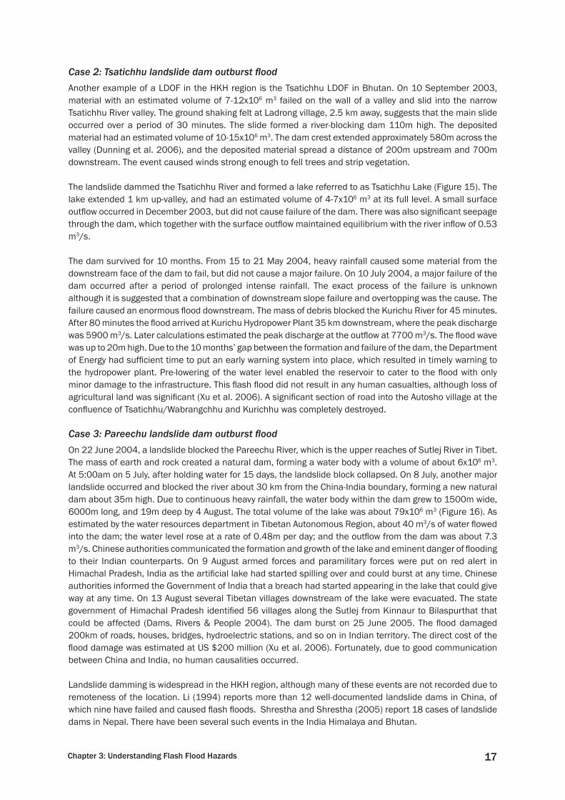
Case 2: Tsatichhu landslide dam outburst fl oodAnother example of a LDOF in the HKH region is the Tsatichhu LDOF in Bhutan. On 10 September 2003, material with an estimated volume of 7-12x106 m3 failed on the wall of a valley and slid into the narrow Tsatichhu River valley. The ground shaking felt at Ladrong village, 2.5 km away, suggests that the main slide occurred over a period of 30 minutes. The slide formed a river-blocking dam 110m high. The deposited material had an estimated volume of 10-15x106 m3. The dam crest extended approximately 580m across the valley (Dunning et al. 2006), and the deposited material spread a distance of 200m upstream and 700m downstream. The event caused winds strong enough to fell trees and strip vegetation.
The landslide dammed the Tsatichhu River and formed a lake referred to as Tsatichhu Lake (Figure 15). The lake extended 1 km up-valley, and had an estimated volume of 4-7x10⁶ m3 at its full level. A small surface outfl ow occurred in December 2003, but did not cause failure of the dam. There was also signifi cant seepage through the dam, which together with the surface outfl ow maintained equilibrium with the river infl ow of 0.53 m3/s.
The dam survived for 10 months. From 15 to 21 May 2004, heavy rainfall caused some material from the downstream face of the dam to fail, but did not cause a major failure. On 10 July 2004, a major failure of the dam occurred after a period of prolonged intense rainfall. The exact process of the failure is unknown although it is suggested that a combination of downstream slope failure and overtopping was the cause. The failure caused an enormous fl ood downstream. The mass of debris blocked the Kurichu River for 45 minutes. After 80 minutes the fl ood arrived at Kurichu Hydropower Plant 35 km downstream, where the peak discharge was 5900 m3/s. Later calculations estimated the peak discharge at the outfl ow at 7700 m3/s. The fl ood wave was up to 20m high. Due to the 10 months’ gap between the formation and failure of the dam, the Department of Energy had suffi cient time to put an early warning system into place, which resulted in timely warning to the hydropower plant. Pre-lowering of the water level enabled the reservoir to cater to the fl ood with only minor damage to the infrastructure. This fl ash fl ood did not result in any human casualties, although loss of agricultural land was signifi cant (Xu et al. 2006). A signifi cant section of road into the Autosho village at the confl uence of Tsatichhu/Wabrangchhu and Kurichhu was completely destroyed.
Case 3: Pareechu landslide dam outburst fl oodOn 22 June 2004, a landslide blocked the Pareechu River, which is the upper reaches of Sutlej River in Tibet. The mass of earth and rock created a natural dam, forming a water body with a volume of about 6x10⁶ m3. At 5:00am on 5 July, after holding water for 15 days, the landslide block collapsed. On 8 July, another major landslide occurred and blocked the river about 30 km from the China-India boundary, forming a new natural dam about 35m high. Due to continuous heavy rainfall, the water body within the dam grew to 1500m wide, 6000m long, and 19m deep by 4 August. The total volume of the lake was about 79x106 m3 (Figure 16). As estimated by the water resources department in Tibetan Autonomous Region, about 40 m3/s of water fl owed into the dam; the water level rose at a rate of 0.48m per day; and the outfl ow from the dam was about 7.3 m3/s. Chinese authorities communicated the formation and growth of the lake and eminent danger of fl ooding to their Indian counterparts. On 9 August armed forces and paramilitary forces were put on red alert in Himachal Pradesh, India as the artifi cial lake had started spilling over and could burst at any time. Chinese authorities informed the Government of India that a breach had started appearing in the lake that could give way at any time. On 13 August several Tibetan villages downstream of the lake were evacuated. The state government of Himachal Pradesh identifi ed 56 villages along the Sutlej from Kinnaur to Bilaspurthat that could be affected (Dams, Rivers & People 2004). The dam burst on 25 June 2005. The fl ood damaged 200km of roads, houses, bridges, hydroelectric stations, and so on in Indian territory. The direct cost of the fl ood damage was estimated at US $200 million (Xu et al. 2006). Fortunately, due to good communication between China and India, no human causalities occurred.
Landslide damming is widespread in the HKH region, although many of these events are not recorded due to remoteness of the location. Li (1994) reports more than 12 well-documented landslide dams in China, of which nine have failed and caused fl ash fl oods. Shrestha and Shrestha (2005) report 18 cases of landslide dams in Nepal. There have been several such events in the India Himalaya and Bhutan.

Resource Manual on Flash Flood Risk Management – Module 218
a.
b.
c.
Figure 15: Tsatichhu landslide dam: a. the source area of the landslide; b. detailed view of the dam; c. Tsatichhu lake
Sou
rce:
Dun
ning
et
al. 2
00
6

19Chapter 3: Understanding Flash Flood Hazards
Figure 16: Satellite image of the Pareechu River: a. about one month after the landslide damming (15 July 2004); b. about 2.5 months after damming (1 September 2004); and c. after the outburst
Sou
rce:
ICIM
OD
; Goo
gle
Eart
h

Resource Manual on Flash Flood Risk Management – Module 220
Case 4: Budhi Gandaki and Larcha Khola in NepalThe Budhi Gandaki River in Nepal was twice dammed near Lukubesi. In 1967, the river was dammed for three days after the failure of Tarebhir. Another landslide in 1968 dammed the river again with a huge amount of displaced material. The river’s water level dropped from a normal level of 4m on 1 August to 0.9m on 2 August. After the breaching of the landslide dam, the water level rose to 14.61m. The peak fl ow was estimated to be 5210 m3/s, which was signifi cantly greater than the mean annual instantaneous fl ood (2380 m3/s). One bridge and 24 houses at Arughat Bazaar, about 22 km downstream from the damming site, were swept away after the breach .
Bhairabkunda Khola was dammed in 1996. The landslide dam outburst fl ood destroyed 22 houses and killed 54 people in Larcha village. The highway bridge was swept away by the fl ash fl ood (Figure 17).
3.3 Glacial Lake Outburst FloodFlash fl oods resulting from the outburst of lakes of glacial origin are called glacial lake outburst fl oods or GLOFs. GLOF is one of the important mechanisms that cause fl ash fl oods in the Himalayas. They are a common phenomenon in Iceland, where the outburst is generally triggered by volcanic action and the phenomenon is known as jokulhaup. Many of the early studies on GLOFs were based in Iceland. Although GLOFs are not a recent phenomenon in the Himalayas, they were only given attention recently, probably because several high-magnitude events caused substantial damage in different parts of the region.
Glacial lakes are directly related to the glacier fl uctuation process, which in turn is attributed to climate variability. The glaciers in the region have been in general retreat since the end of the Little Ice Age of the mid-19th Century. However, the retreat has accelerated in recent decades, most probably due to anthropogenic
a. b.
c. d.
Figure 17: a. Bhairabkunda Khola a few days after the LDOF; b. debris deposited by the LDOF; c. large boulders trapped at the highway bridge; and d. Larcha village destroyed by the fl ash fl ood
N.R
. Kha
nal,
TU

21Chapter 3: Understanding Flash Flood Hazards
climate change, which is highly pronounced in the region. The retreat of glaciers leaves behind large voids to be fi lled by meltwater, thus forming moraine-dammed glacial lakes. These natural moraine dams are composed of unconsolidated moraines of boulders, gravel, sand, and silt. The dams are structurally weak and unstable, and undergo constant changes due to slope failures, slumping, and similiar effects and are in danger of catastrophic failure, causing glacial lake outburst fl oods. Moraine dams may break by the action of some external trigger or by self-destruction (Table 2). A huge displacement wave generated by a rockslide or snow/ice avalanche from the glacier terminus into the lake may cause the water to overtop the moraine, create a large breach, and eventually cause dam failure (Ives 1986). Earthquakes may also trigger dam breaks depending upon magnitude, location, and characteristics. Self-destruction is caused by the failure of the dam slope and seepage from the natural drainage network of the dam.
3.4 Types of Glacial LakesGlacial lakes formed as a result of damming material are widely divided into two categories: ice-dammed lakes and moraine-dammed lakes. Ice-dammed lakes are created when a stream is intercepted by a glacier, often during the advance stage, while moraine-dammed lakes are confi ned by moraines left by retreat of the parent glacier. Ice-dammed lake failure is a complicated process and the resulting fl ood discharge is less ‘spiky’, whereas moraine-dammed lake outbursts cause sharp rises and falls in fl ood discharge.
Depending on the juxtaposition of the lake with respect to the glacier, the lakes can be supraglacial, englacial, or marginal. Figures 18 and 19 show schematic and real representations of typical locations of ice-dammed and moraine-dammed lakes.
Table 2: GLOF triggering mechanisms
Internal External
Hydrostatic pressure (increase in water level)
Overtopping of moraine dam due to rock, ice, snow avalanche into the lake
Seepage Earthquake Destruction of conduits within ice core
Figure 18: Types of glacial lakes
Glacier
Lake
River
River Valley
Flow Direction
I
MI/B
I/B
S
I/CI/Ig
I/MgSymbol Type of Lake
I Ice-dammed lakeM Moraine-dammed lakeS Supraglacial lakeB Lake dammed by tributary glacier (blocked lake)C Converging ice pondedIg Interglacial pondedMg Marginal ponded
Note: Two letter symbol means both apply, (e.g., A/D means ice-dammed lake with the damming caused by a tributary glacier)

Resource Manual on Flash Flood Risk Management – Module 222
3.5 Glacial Lake Outburst Flood in the HKH RegionThere have been at least 35 recorded GLOF events in the HKH region: 16 in China, 15 in Nepal, and four in Bhutan. There have been some reports of fl oods of glacial origin in India and Pakistan, but details of the sources and mechanisms are not available. Many of the GLOFs in China occurred in the southern part of the Tibetan Plateau, where rivers drain into Nepal. Ten of these events led to transboundary damage and many caused major damage in Nepal. One of the most remarkable in this context is the Zhangzanbo lake GLOF of 11 July 1981. The lake burst due to a sudden ice avalanche. A breach 50m deep and 40-60m wide formed at the moraine. The peak discharge of the burst at the outlet was about 16,000 m3/s. The main fl ood lasted for an hour, during which time an estimated 19 million m3 of lake water drained. This GLOF created a great change in the landform downstream due to erosion and sedimentation, and caused considerable damage to the highway below the lake up to the Sunkoshi power station. It destroyed the friendship bridge between Nepal and China and two other bridges, one in Tibet and one in Nepal (Figure 20). The fl ood caused heavy damage to the diversion weir of Sunkoshi hydropower station.
Glacier
Gla
c ie r
Glacier
LakeLake
Lake
Mo
rain
eMo
ra ine
NaturalOut let
Figure 19: Typical ice-dammed (left) and moraine-dammed (right) lakes
Sou
rce:
Yam
ada
19
98
Figure 20: Remnants of a bridge pier (left) on the Arniko Highway and a section of the highway destroyed by the 1981 Zhanzangbo GLOF
Sou
rce:
Moo
l et
al. 2
001

23Chapter 3: Understanding Flash Flood Hazards
One of the region’s best-documented GLOF events is the Dig Tsho GLOF of 4 August 1985. Dig Tsho lake is located at the headwaters of the Bhotekoshi, a tributary of the Dudhkoshi River. The lake is in contact with Langmoche, a steep glacier. The GLOF destroyed the nearly complete Namche hydropower project. In addition, the GLOF destroyed 14 bridges, trails, and cultivated land, and caused the loss of many lives. The total damage was estimated at US $1.5 million. Figure 21 shows the Dig Tsho Lake before and after the burst.
b.
c. e.
d. f.
a.
Figure 21: a. Dig Tsho lake after the GLOF outburst in 1985; b. the fl ash fl ood caused by the Dig Tsho outburst; c. the end moraine of Dig Tsho before the breach; and d. after the breach; e. the Namche hydropower station site before; and f. after the outburst
Sou
rce:
Moo
l et
al. 2
001

Resource Manual on Flash Flood Risk Management – Module 224
How do humans contribute to fl ooding?
Floods are a naturally occurring hazard that become disasters when they affect human settlements. The magnitude and frequency of fl oods is often increased as a result of the following human actions.
Settlement on fl oodplains contributes to fl ooding disasters by endangering humans and their assets. However, the economic benefi ts of living on a fl oodplain outweigh the dangers for some communities. Pressures from population growth and shortages of land also promote settlement on fl oodplains. Floodplain development can also alter water channels, which if not well planned can contribute to fl oods.
Urbanisation contributes to urban fl ooding in four major ways. Roads and buildings cover the land, preventing infi ltration so that runoff forms artifi cial streams. The network of drains in urban areas may deliver water and fi ll natural channels more rapidly than naturally occurring drainage, or may be insuffi cient and overfl ow. Natural or artifi cial channels may become constricted due to debris, or obstructed by river facilities, impeding drainage and overfl owing the catchment areas.
Deforestation and removal of root systems increases runoff. Subsequent erosion causes sedimentation in river channels, which decreases their capacity.
Failure to maintain or manage drainage systems, dams, and levee bank protection in vulnerable areas also contributes to fl ooding.

25Chapter 4: Flash Flood Risk Assessment
Chapter 4Flash Flood Risk Assessment
Risk assessment forms the core of the fl ash fl ood risk management process. Risk assessment helps identify potential risk-reduction measures. If integrated into the development planning process, it can identify actions that both meet development needs and reduce risk. Flash fl ood damage can be reduced by establishing a proper fl ood control management structure or organ to manage fl ood events and reduce their negative effects. The benefi ts of precautionary steps, measures, and actions will bring communities, agricultural land, infrastructure, and livelihoods in fl ash fl ood-prone areas to safety with the help of government management.
4.1 What is Risk?The term risk has a range of meanings depending on the specifi c sector in which it is used — for example, the economic, environmental, or social sector. Because the terminology of risk has been developed across a wide range of disciplines and activities, there is potential for misunderstanding of the technical terminology associated with risk assessment, as technical distinctions are made between words which in common usage are normally treated as synonyms. Most important is the distinction that is drawn between the words hazard and risk.
This manual uses the Source-Pathway-Receptor-Consequence (S-P-R-C; Figure 22) concept proposed by Gouldby and Samuals (2005): For a risk to arise there must be hazard, which is the source or initiator event (e.g., cloudburst); pathways between the source and receptors (e.g., fl ood routes, overland fl ow, or landslide); and receptors (e.g., people and property). The consequence depends on the exposure of the receptors to the hazard.
The evaluation of risk requires consideration of the following components: the nature and probability of the hazard (p); the degree of exposure of the receptors (number of people and property) to the hazard (e); the susceptibility of the receptors to the hazards (s); and the value of the receptors (v).
Therefore Risk=ƒ(p, e, s, v)
The fi rst two components of risk are related to hazard and the last two components to vulnerability. In the functional form,
Vulnerability = ƒ(s, v)
Thus, vulnerability is a sub-function of risk. This term describes the predisposition of a receptor to suffer damage.
Risk is, therefore, a statistical concept and is the probability that a negative event or condition will affect the receptor in a given time and space. Thus, risk can be understood in simple terms as:
Risk = (Probability) x (Consequence)
SOURCE
e.g., intense rainfall, displacement wave,
landslide blocking riverflow
PATHWAY(s)
e.g., dam breach, inundation, overflow
RECEPTOR(s)
e.g., people, infrastructure, property,
environment
CONSEQUENCE
e.g., loss of life, stress, material damage,
environmental degradation
Figure 22: Source-Pathway-Receptor-Consequence conceptual model

Resource Manual on Flash Flood Risk Management – Module 226
The degree of fl ood hazard in an area is often measured by the return period of the fl ood, which relates to the probability of the fl ash fl ood hazard. Management of fl ash fl ood risk can be accomplished by managing hazard, exposure, and vulnerability. Here vulnerability encompasses both physical and social vulnerabilities. Flash fl ood risk management can be done through structural measures, which alter the frequency (i.e., the probability) of fl ood levels in the area. On the other hand, fl ash fl ood management can also be done through non-structural measures that focus on the exposure and vulnerability of a community to fl ash fl ood. Changing or regulating land use, installing an early warning system, and developing the community’s resilience are examples of non-structural measures.
4.2 Major Steps in Flash Flood Risk AssessmentRisk assessment forms the core of the disaster risk management process and results in the identifi cation of potential risk-reduction measures. Risk assessment integrated into the development planning process can identify actions that both meet development needs and reduce risk. Identifi ed risk-reduction actions can be incorporated into development policies and legal arrangements. For example, policies and associated laws and regulations to reduce the risk of fl ash fl oods can require or encourage construction of spurs or embankments as part of road or water resources projects.
Risk assessment is an essential part of the fl ash fl ood risk management decision-making process. A number of methods have been developed to assess the risk of natural disasters. Here, we have adopted the method developed by Colombo et al. (2002), and Gouldby and Samuals (2005), after appropriate modifi cation (Figure 23). Risk assessment steps include: 1. characterising the area2. assessing hazard or determining hazard level and intensity3. assessing vulnerability4. assessing risk
4.3 Characterisation of the Risk-prone AreaThis process comprises three main topics: the information to be collected on the area prone to fl ash fl oods; the tools to be used for collection, processing, and archiving the information; and the format for documentation.
Information to be collectedThe information to be collected to characterise a fl ash fl ood-prone area must fulfi l two main tasks: it must provide scientifi c data for hazard, vulnerability, and risk analysis, and it must assist decision-makers during the subsequent planning process. Characterising the area is important for both hazard and vulnerability assessment. For this, the following information should be collected.
Geography (physical and social): ● for example, the length of river sections, communities/provinces involved, peculiarities of the area, and population and population distribution
Geology and geomorphology: ● the properties of rocks and soil in the area, river courses or pathways
Hydrology and hydraulics: ● the properties of the rivers and waterways in the area such as fl ow amount, cross-sections, and slope
Hydrometeorology: ● for example, air temperature, annual precipitation, months of maximum and minimum precipitation, values of precipitation extremes
Area
characterisation
Hazard
analysis(hazard intensity)
Probablity
assignment
Hazard
assessment(hazard level)
Vulnerabilty
analysis
Risk
assessment
Figure 23: Procedural diagram for fl ash fl ood risk analysis

27Chapter 4: Flash Flood Risk Assessment
Vegetation: ● types of plants and trees that grow in the area
Land use: ● land use types such as agricultural land, forest and other wooded land, built-up and related land, wet open land, dry open land with special vegetation cover, open land with or without signifi cant vegetation cover
Existing counter-measures: ● for example, check dams and bioengineering work
Historical analysis of local fl ood events: ● for example, fl oods that have happened in the past; sources of information include local memory, damaged environment, national and local databanks, newspapers, and interviews with victims
Tools for collecting, processing and archiving informationThree main tools are useful in characterising the area subject to fl ash fl oods:1. database for storing general information2. a geographic information system (GIS) for graphical representation of maps and spatial analysis3. a set of computer programs for data processing (e.g., hydrological and hydraulic models)
Format for documentationFlash fl oods in the HKH region are generally spatially limited and often occur in remote and isolated locations, frequently going undocumented. Even documented events often lack information vital for risk analysis. Thus, it is extremely useful to develop a comprehensive standardised format to facilitate further analysis of data. Such a format will enhance information sharing among institutions, communities, and countries in the region. Event documentation should include the following information:
Location of the event: ● geographic coordinates of settlements in the vicinity of the source, as well as the impacted areas
Basin details: ● description of the drainage system, the river/stream where the event occurred, the major river basin that the river/stream drains into
Cause of event: ● heavy rainfall, GLOF, LDOF, etc.
Hydrometeorological details: ●amount and duration of rainfall including peak hourly intensities –amount of water released by LDOF or GLOF –duration of fl ood –peak fl ood discharge –
Extent of damage: ●dead –injured –missing –agriculture –infrastructure –homesteads –businesses –cattle –affected area, people, families –
Damage in monetary terms ●
4.4 Hazard AnalysisThis process includes defi ning fl ash fl ood hazard intensity (the strength of the fl ash fl ood), and describing alternative scenarios in their catchments. Determining hazard intensity is a step towards determining hazard levels. It is common to present hazard scenarios in the form of hazard maps. Modern technology has advanced hazard mapping and the prediction of future events considerably through techniques such as geological mapping and satellite imagery, production of high resolution maps, and computer modelling. New geographic information system (GIS) mapping techniques, in particular, are revolutionising the capacity to prepare hazard

Resource Manual on Flash Flood Risk Management – Module 228
maps. It is, however, essential to verify the maps through fi eld observation. Often hazard maps can be prepared with community involvement, and the best results can be achieved by combining the technical hazard maps with others prepared by the community. This process includes defi ning fl ash fl ood hazard intensity and possible scenarios in their catchments. A simple way of assigning fl ash fl ood hazard intensity is shown in Table 3, although in reality determining hazard intensity is much more complicated. Alternatively, hazard intensity can be determined by the level of anticipated fl ooding. Figure 24 shows an example of a fl ood hazard map.
Assigning probability to a hazard scenarioThe hazard scenario should be assigned probability levels. In the case of intense rainfall fl oods, the return period or frequency of the rainfall events, or the return period or frequency of fl ooding caused by these events, can be used to give probability levels as shown in Table 4.
It is diffi cult to assign probability levels to other types of fl ash fl oods such as LDOF and GLOF, as they often occur only once. In such cases it is customary to use probability levels based on the characteristics of the lake, dam, or surrounding environment, as shown in Table 5.
4.5 Hazard AssessmentHazard assessment includes determining the hazard level scale by combining the hazard intensity based on the hazard intensity scenario and the hazard probability level. Figure 25 shows an example of a hazard level scale. The hazard probability has four levels and the hazard intensity level has four degrees (high, moderate, moderately low, low). The resulting 16-cell hazard level scale identifi es four different levels (very high, high, moderate, and low).
Figure 24: A simple fl ood hazard map of Bhandara Village Development Committee area, Chitwan, Nepal
Sou
rce:
ICIM
OD
Table 3: A simple way of assigning hazard intensity
Hazard intensityDanger to population close to the stream
Danger to population in settlement (about 500m
from the stream)
Danger to population 1 km away from the
stream
Danger to population more than 1 km away from the stream
High yes yes yes yes
Moderate yes yes yes no
Moderately Low yes yes no no
Low yes no no no

29Chapter 4: Flash Flood Risk Assessment
Table 4: Probability level of a hazard scenarioProbability level Frequency
High at least once in 10 years
Moderate once in 10 to 30 years
Moderately Low once in 30 to 100 years
Low less frequent than once in 100 years
4.6 Vulnerability AssessmentThe next step in risk analysis is the vulnerability assessment. There are three schools of thought on vulnerability analysis. The fi rst focuses on exposure to biophysical hazards, including analysis of the distribution of hazardous conditions, human occupancy of hazardous zones, degree of loss due to hazardous events, and analysis of the characteristics and impacts of hazardous events (Heyman et al. 1991; Alexander 1993; Messner and Meyer 2005). The second looks at the social context of hazards and relates social vulnerability to coping responses of communities, including societal resistance and resilience to hazards
Figure 25: Hazard level scale
Table 5: Probability level for LDOF and GLOFIndicator Characteristic Qualitative probability
Type of dam
ice high
moraine medium high
bedrock low
Freeboard relative to dam
low high
medium medium
high low
Dam height to width ratio
large high
medium medium
small low
Impact waves by ice/rock falls reaching the lake
frequent high
sporadic medium
unlikely low
Extreme meteorological events (high temperature/ precipitation)
frequent high
sporadic medium
unlikely lowSource: RGSL (2003)
High ModerateModerately
lowLow
High
Moderate
Moderately
low
Low
Hazard
Inte
nsity
Probability Level
Hazard level
Very High
High
Moderate
Low
Resource Manual on Flash Flood Risk Management – Module 230
(Blakie et al. 1994; Watts and Bohle 1993; Messner and Meyer 2005). The third combines both approaches and defi nes vulnerability as a hazard of place, which encompasses biophysical risks as well as social response and action (Cutter 1996; Weichselgartner 2001; Messner and Meyer 2005). The third school has become increasingly signifi cant in the scientifi c community in recent years and this manual is based on this approach.
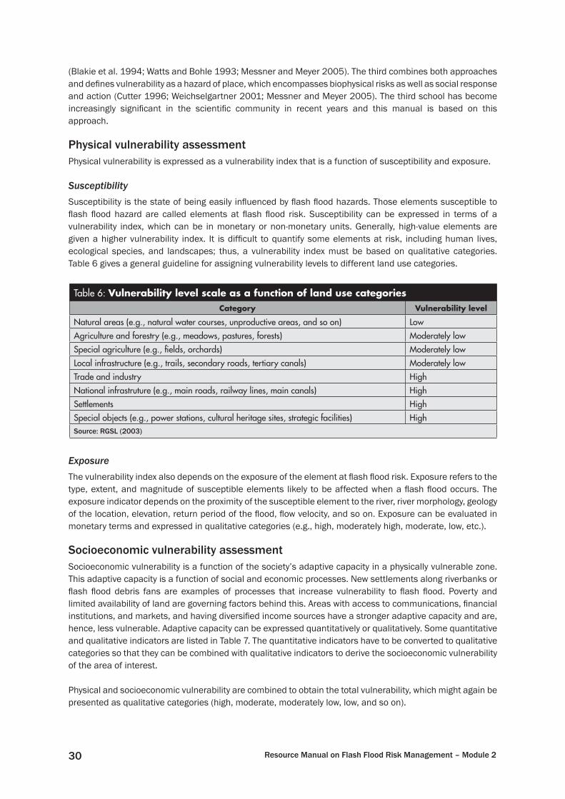
Physical vulnerability assessmentPhysical vulnerability is expressed as a vulnerability index that is a function of susceptibility and exposure.
SusceptibilitySusceptibility is the state of being easily infl uenced by fl ash fl ood hazards. Those elements susceptible to fl ash fl ood hazard are called elements at fl ash fl ood risk. Susceptibility can be expressed in terms of a vulnerability index, which can be in monetary or non-monetary units. Generally, high-value elements are given a higher vulnerability index. It is diffi cult to quantify some elements at risk, including human lives, ecological species, and landscapes; thus, a vulnerability index must be based on qualitative categories. Table 6 gives a general guideline for assigning vulnerability levels to different land use categories.
ExposureThe vulnerability index also depends on the exposure of the element at fl ash fl ood risk. Exposure refers to the type, extent, and magnitude of susceptible elements likely to be affected when a fl ash fl ood occurs. The exposure indicator depends on the proximity of the susceptible element to the river, river morphology, geology of the location, elevation, return period of the fl ood, fl ow velocity, and so on. Exposure can be evaluated in monetary terms and expressed in qualitative categories (e.g., high, moderately high, moderate, low, etc.).
Socioeconomic vulnerability assessmentSocioeconomic vulnerability is a function of the society’s adaptive capacity in a physically vulnerable zone. This adaptive capacity is a function of social and economic processes. New settlements along riverbanks or fl ash fl ood debris fans are examples of processes that increase vulnerability to fl ash fl ood. Poverty and limited availability of land are governing factors behind this. Areas with access to communications, fi nancial institutions, and markets, and having diversifi ed income sources have a stronger adaptive capacity and are, hence, less vulnerable. Adaptive capacity can be expressed quantitatively or qualitatively. Some quantitative and qualitative indicators are listed in Table 7. The quantitative indicators have to be converted to qualitative categories so that they can be combined with qualitative indicators to derive the socioeconomic vulnerability of the area of interest.
Physical and socioeconomic vulnerability are combined to obtain the total vulnerability, which might again be presented as qualitative categories (high, moderate, moderately low, low, and so on).
Table 6: Vulnerability level scale as a function of land use categoriesCategory Vulnerability level
Natural areas (e.g., natural water courses, unproductive areas, and so on) Low
Agriculture and forestry (e.g., meadows, pastures, forests) Moderately low
Special agriculture (e.g., fi elds, orchards) Moderately low
Local infrastructure (e.g., trails, secondary roads, tertiary canals) Moderately low
Trade and industry High
National infrastruture (e.g., main roads, railway lines, main canals) High
Settlements High
Special objects (e.g., power stations, cultural heritage sites, strategic facilities) HighSource: RGSL (2003)

31Chapter 4: Flash Flood Risk Assessment
4.7 Risk AssessmentA risk-level scale is a combination of hazard level and total vulnerability (both physical and socioeconomic). The scale is obtained by subjective judgment, similar to the hazard-level scale. Figure 26 shows a risk-level scale that can be used to assess fl ash fl ood risk. Four levels of hazard and four levels of total vulnerability (high, moderate, moderately low, and low) are considered. The resulting risk-level scale consists of 16 cells and may be classifi ed into fi ve different risk levels: very high, high, moderate, moderately low, and low.
The methodology presented in this section is one of many available in the literature or, rather, it is a combination of several methodologies. It may be modifi ed or simplifi ed according to need, resources available, and data available. Annex 16 provides an exercise on hazard vulnerability and risk assessment. The ILWIS7 3.2 based exercise uses multiple hazards instead of a single hazard. In reality, communities are exposed to different types of hazards and stresses.
6 The exercise was provided by C.J. van Westen, International Institute for Geo-Information Science and Earth Observation (ITC) and is available from <http://www.itc.nl/ilwis/applications/application01.asp> (Accessed October 2007).7 An open source version, ILWIS 3.4 Open, can also be used. It is freely downloadable from <http://52north.org/index.php?option=com_projects&task=showProject&id=30&Itemid=127>.
Figure 26: Classifi cation of risk level
Risk level
High ModerateModerately
LowLow
High
Moderate
Moderately
Low
Low
Vulnerability Level
Ha
zard
Le
vel
Very High
High
Moderate
Moderately Low
Low
Table 7: Quantitative and qualitative indicatorsParameter Quantitative indicators
Accessibility Road density (m/km2)
Health Number of health institutions/1000 population
Communications Number of telephones/1000 population
Institutions Number of GOs and NGOs/1000 population
Economic Number of fi nancial institutions/1000 population
Loss-sharing measures Value of revolving fund (disaster fund)
Economic diversity Percentage of families with a number of income sourcesQualitative indicators
Emergency facilities
Warning system
Loss reduction measures
Awareness and attitudeSource: Shrestha (2005)

33Chapter 5: Flash Flood Risk Management
Chapter 5Flash Flood Risk Management
Flash fl ood risk management can include structural and non-structural measures. A common strategy to cope with fl oods has been to construct civil works such as fl oodwalls, transversal protection works, embankments, conduits, and reservoirs to protect the environment up to an acceptable risk threshold. Structural measures tend to consider mainly the hydrological and hydraulic implications of fl ooding, which are generally solved by choosing the alternative that maximises the expected net benefi t. In addition, such measures can have a substantial impact on the riverine environment and ecology. Furthermore, while structural solutions contribute to fl ood reduction and protection, they also have hidden ‘piggy-back’ liabilities associated with them, such as the issue of their long-term value, the false sense of security they may provide, their possible environmental impact, and costs related to their operation and maintenance.
In contrast, non-structural measures (see below) offer a variety of possibilities, ranging from land use planning and construction and structure management codes, through soil management and acquisition policies, insurance, and perception and awareness, to public information actions, emergency systems, and post-catastrophe recovery, all of which contribute towards the mitigation of fl ood-related problems. The advantage of non-structural measures is that, generally, they are sustainable and less expensive. Table 8 gives some examples of structural and non-structural measures. Non-structural measures are often the most effective in managing fl ash fl oods. However, they can only be effi cient with the participation of a responsive population and an organised institutional network. A combination of structural and non-structural measures can be the best. This manual deals explicitly with the non-structural measures for fl ash fl ood risk management.
Table 8: Structural and non-structural measures for fl ash fl ood risk management
Structural measures
Catchment-wide interventions (agriculture and forestry actions and water control works)
River training interventions
Other fl ood control interventions (passive control, water retention basins and river corridor enhancement, rehabilitation and restoration)
Non-structural measures
Risk acceptance
Tole
renc
e str
ateg
ies Toleration
Emergency response system
Insurance
Risk reduction
Prev
entio
n str
ateg
ies
Watershed management
Delimitation of fl ood areas and securing fl ood plains
Implementation of fl ood area regulations
Application of fi nancial measures
Miti
gatio
n str
ateg
ies
Reduction of discharge through natural retention
Forecasting and early warning
Emergency action based on monitoring, warning, and response systems (MWRS)
Public information and educationSource: Colombo et al. (2002)

Resource Manual on Flash Flood Risk Management – Module 234
5.1 Non-structural MeasuresThe need for non-structural measures becomes very important when dealing with settled areas, as they allow control of the vulnerability component of fl ood risk (see Chapter 4).
Non-structural measures are particularly important for the HKH region for several reasons:the high cost and short lifetime of structural measures ●lack of capacity to build and operate structural measures ●low involvement of local community, lack of feeling of ownership ●other environmental impacts of structural measures ●
Non-structural measures tend to be more sustainable because they include the active involvement of the community. National and regional policy should favour non-structural alternatives due to their low cost and reduced number environmental side effects, and implement structural measures only as a last resort.
Non-structural measures can be grouped into two categories: risk acceptance and risk reduction measures.
Risk acceptanceAcceptable risk is the level of loss a society or community considers acceptable given existing social, economic, political, cultural, technical, and environmental conditions (UN/ISDER terminology8).
Risk acceptance implies that the government or community accepts a degree of human and material loss due to a fl ash fl ood that could impact the area in the short-, medium-, and long-term. There are mainly three types of risk acceptance strategies: toleration, emergency response system, and insurance.
TolerationToleration of risk implies that a competent authority (local, regional, or national) accepts that fl ash fl oods occur. Generally, proactive initiatives will not be carried out other than, perhaps, a risk analysis (see example in Annex 1). In this case, it is very likely that the competent authority will accept the results of the risk assessment and not promote any complementary activities. Although risk analysis is gradually gaining ground with competent authority routines, it still needs to become common practice.
Emergency response systemsThe use of emergency response systems implies that the local, regional, or national competent authority is aware that their area of jurisdiction is prone to fl ash fl oods. Risk assessment and modelling, coupled with mapping, is probably carried out, but fl ash fl oods will mainly be dealt with via the elaboration of emergency plans and using already existing structures.
All emergency plans (regional, district, local) should be based on a national emergency plan in order to carry out the same doctrine of civil protection emergency operations within a particular country in a concerted manner. In general, the various public authorities taking part in the emergency plan will play roles related to their day-to-day responsibilities. They must prepare themselves according to the mission statement established in the emergency plan. To achieve this, each competent authority (regional, district, local) must have its own emergency plan, accompanied by an operations manual. Furthermore, each collaborative unit (police, fi re brigade, hospital, and so on) should also have its own emergency plan and operations manual.
InsuranceInsurance against fl ash fl ood damage should be an integral part of risk acceptance. However, many countries in the HKH region still do not use fl ood insurance due to its high cost. Existing solutions to fl ood coverage are
8 UN/ISDR terminology of disaster risk reduction (http://www.unisdr.org/eng/library/lib_terminology_eng%20home.htm; Accessed June 2007).

35Chapter 5: Flash Flood Risk Management
quite diverse, mainly due to the technical diffi culties involved in providing insurance cover against fl ooding, differing views on the role of the state in managing fl ood risk, and last but not least, diverging perceptions of the dangers posed by fl ooding. The solutions in place range from unrestricted private insurance coverage to state aid for fl ood victims.
Insurance companies have various instruments available to cover the risk. Some examples are given below.
In combination with other natural perils: ● Flood risk is usually covered in combination with other natural perils in order to appeal to as many customers as possible, achieve maximum market penetration, and minimise the risk of selection bias.
Grouping of several insurance portfolios in a pool: ● Flood risk is spread among other insurance portfolios and is offered as a package. This also decreases the risk to the insurer.
Resilient reinstatement: ● Flood insurance is made available only to fl oodplain residents who make an effort to make their houses more resistant to fl ooding (e.g., use of fl ood-resistant products and techniques when repairing a fl ood-damaged property, installing electrical sockets one metre above the fl oor instead of just above the skirting board).
Generally there is diffi culty in dividing the risk fairly among the parties involved (i.e., the property owner, (re)insurer, and the state). This is mainly due to the very different hazard potentials in play and the differences in perception of these hazards. Furthermore, the system of insurance policies applied only on a local level is far too expensive both for insurance companies and for private and public entities. The following recommendations may help overcome these problems:
A mandatory national or regional (e.g. South Asian Association for Regional Cooperation [SAARC], HKH) ●insurance fund against natural hazards should be established, so as to spread costs. This would follow the concept of joint sharing of burdens and would reduce the costs of expensive disaster-relief payments.
The development of risk-oriented models for determining the implications of a fl ood hazard should be ●promoted and funded. This would require an external source of funds additional to insurance, which could raise data-protection problems.
5.2 Risk ReductionSuccess in managing fl ood areas depends on selecting suitable measures based on fl ood characteristics, physical and morphological characteristics of fl ood areas, economic and social conditions, political and environmental conditioning, or fl ood-control works planning. Structural measures cannot reach these objectives if they are used alone; non-structural measures such as land use control and planning can be tools not only to reduce fl ood risk, but also to develop a sustainable approach to fl ood management. Risk reduction is one of the main goals in fl ash fl ood management. It can be dealt with in two ways: prevention strategies and mitigation strategies. The following section describes different approaches, tools, and activities for fl ash fl ood risk reduction.
Watershed management9
Watershed management has both structural and non-structural components. Non-structural components can be important measures in reducing fl ash fl ood risk. Watershed management is a cross-cutting exercise closely related to socioeconomy and development. Watershed management should consider a number of basic principles related to runoff and erosion including soil, topography, land cover and use, and farming practices.
9 This section includes contributions from Keshar Man Sthapit, ICIMOD.

Resource Manual on Flash Flood Risk Management – Module 236
The following measures in a watershed can signifi cantly reduce the risk of fl ash fl oods (Figure 27):
Agricultural measures: ● Agricultural activities should minimise the generation of runoff and sediment. Contouring and terracing of upland farms is a good measure to ensure this. Crops should be selected to ensure longer coverage, especially in rainy periods. Conversion into arable land should be avoided where slopes exceed 25%. Agricultural practices that increase organic matter in the soil should be favoured.Remodelling of agriculture: ● Agriculture in fl ood-prone areas should be conducted in ways that minimise the fl ood damage to crops. Assam, where fl oods occur regularly, provides a good example of what can be done. The successive waves of fl oods from the Bhrahmaputra and Barak rivers and their tributaries cause extensive damage to agriculture (Figure 28):
The ahu crop (rice) is damaged –before the harvest.The sali or main crop of rice cannot –be transplanted in time as the seedlings are damaged either in the nursery or after transplanting, sometimes even destroyed in the fi eld.The jute crop is damaged or quality is –adversely affected, and so on.
Various strategies are used related to remodelling of land use to minimise the adverse effects of recurrent fl oods (Swaminathan 1980):
Multiple cropping: ● Cropping of medium tall ahu rice with deep-water rice in low-lying areas as an insurance so that if the ahu rice is damaged, there will be some production from the deep-water rice.Restructuring of the cropping pattern: ● The safest way to assure crop production in fl ood-prone areas is to use the fl ood-free period for growing crops. Figure 28 shows the fl ood-free period and the potential for growing crops in this period.Forestry: ● Reforestation can be a good measure to decrease runoff. Tree species that do not prohibit undergrowth should be selected. Logging should be carried out during non-rainy seasons. Plan for log-skidding tracks, as they might trigger fl ash fl oods. Favour mixed, uneven aged, and autochthonous woods by selective thinning and coppicing.Rangeland management: ● Pasture renewal through fi re should be avoided as this reduces soil organic matter. Grazing should be regulated through the correct assessment of optimum livestock numbers. A more homogeneous distribution of livestock and use of rotation grazing methods should be encouraged.
Rangeland managementPrevents overgrazing, decreases runoff
Flood plainAllows flood to pass safely
TerracingDecreases runoff,reduces erosion
PondingSlows water velocity, reduces erosion
Contouring of farmlandControls water flow, reduces erosion
Settlement locationMinimises flash flood damage
ReforestationDecreases runoff
Figure 27: Some aspects of watershed management
FEB MAR APR MAY JU
N JUL AUG
SEP
OCT
NO
V
D
EC
JAN
WHEATBLA
CK &
GRE
EN G
RA
M
MU
STARD
AH
U RIC
E P
OTA
TO
BORO RICE
LEN
TIL
GREEN G
RAM
RI
CE
(SA
LI) JU
TE
VEGETABLE
FLOOD
Figure 28: Modifi cation of cropping pattern to suit fl ooding period
Sou
rce:
Mod
ifi ed
from
DM
TP 1
997
Sou
rce:
Mod
ifi ed
from
Sw
amin
atha
n 1
98
0

37Chapter 5: Flash Flood Risk Management
Floodplain management: ●Floodplain management includes fl ash fl ood hazard mapping, which shows the areas that will be –impacted by a fl ood of a particular return period and enables delimitation of fl ood areas. Flood hazard mapping can be conducted to different degrees of detail. A very simple fl ood hazard map shows the area of inundation. In addition, the depth of inundation, the velocity of fl ood water at a given location, elements at risk, and others can be provided. A simple exercise on GIS-based fl ood hazard mapping is provided in Annex 210.One important activity is the delimitation of fl ood areas and securing of fl ood plains. Based on the –technical study on fl ash fl ood hazard mapping, streams should have adequate buffer areas to safely cater for fl ood waves. The fl oodplain can be divided into: 1) critical zone (waterway); 2) restrictive zone; 3) regulatory zone; and 4) warning zone (Figure 29). Zone 1 is the waterway/river channel that gets fl ooded every year and where any human interference should be prohibited. Where a river has right of way, humans should stay out of its way. Zone 2 gets fl ooded every three to fi ve years, and construction should be restricted and only agriculture permitted. Every 3-5 years one crop will be lost due to fl ood and there will be harvests in fl ood-free years. In Zone 3, construction should have adequate protection measures such as embankments, fl ood proofi ng, and so on. Zone 4 experiences fl ooding more rarely, averaging once every 25 years. Construction in the area should have tolerance against fl ash fl oods. Flood warning plays an important role here. Natural ponds in the watershed retain the runoff and dampen the peak discharges in the stream. –The ponds should be maintained properly and fi lling the depressions for development purposes should be avoided.Incentive policies should be created and promulgated to achieve better control of building in fl ash –fl ood-prone areas. Examples of such an incentive policy would be granting building permits that are linked to runoff conditions, and relocation grants to move houses from the fl oodplain.Watershed committees. Legislation should incorporate fl ash fl ood related issues within the framework –of watershed committees. This is important because of the interdisciplinary implications of fl ash fl ood management.
(4) Warning ZoneBased on technical study,
outer limit of floodway fringe
(2) Restrictive ZoneKept open to carry flood water,
no building, no fill
(3) Regulatory ZoneUse permitted if protected by embankments,
flood proofed, or otherwise protected
(1) WaterwaysKeep away to allow river to flow
Figure 29: An example of fl oodplain zoning
Sou
rce:
Mod
ifi ed
from
DM
TP 1
997
10 The exercise was developed by the Asian Disaster Preparedness Center (ADPC) based on a case study from Sri Lanka. The exercise is based on ILWIS software. An open source version, ILWIS 3.4 Open, can also be used. It is freely downloadable from <http://52north.org/index.php?option=com_projects&task=showProject&i d=30&Itemid=127>.

Resource Manual on Flash Flood Risk Management – Module 238
Land use control: ● Land use control has much in common with fl oodplain management; it should also be implemented in conjunction with a technical study on fl ash fl ood hazard mapping. Land use regulation is designed to reduce danger to life, property, and development when fl ash fl oods occur. The following elements should be addressed while implementing land use control in a watershed. Many of the elements mentioned here are directly related to planning and policy makers, although fl ash fl ood managers should also have a good understanding of these issues.
Reduction of densities: In fl ash fl ood prone areas, the number of casualties is directly related to the –population density of the neighbourhood at risk. If an area is still in the planning stage, regulation of densities may be built into the plan. For already settled areas, especially squatter settlements, regulation of density can be a sensitive issue and has to address the socioeconomic implications of resettlement. Unfortunately, many situations exist where dense unplanned settlements are located on fl oodplains. Planners must incorporate measures to improve sites and reduce vulnerability.Prohibiting development in areas of high risk: No major development should be permitted in areas –subject to fl ooding once every 10 years on average. Areas of high risk can be used for functions with a lower risk potential such as nature reserves, sports facilities, and parks. Functions with high damage potential such as hospitals should be permitted in safe areas only. Relocation of elements that block the fl ood passage: In addition to the obvious danger of being –damaged or washed away, buildings and other structures blocking the fl oodway may cause damage by trapping fl oodwaters which then overfl ow into formerly fl ood-free zones.Implementation of a building code: The design of buildings and choice of building materials should –consider the probability and severity of fl ash fl oods.Provision of escape routes: Land use plans should have clear escape routes and provide refuge –areas on higher ground.
Integrated fl ash fl ood managementParadigm change in fl ood managementFlood management has traditionally been problem driven, with more activities implemented after a severe fl ood. Actions generally have included structural and non-structural, physical and institutional fl ash fl ood management interventions implemented before, during, and after the fl ash fl ood or other event. Often fl ood management has involved confl ict with other sectors such as building, agriculture, and water resource management. Flood has been treated as a negative phenomenon and its positive aspects largely ignored, although the ecosystem services provided by fl oods are very important. Some fl ood management interventions even adversely impact on riverine ecosystems.
Climate change projections suggest there will be an increased frequency and an increase in magnitude of fl ash fl oods, and a wider distribution of these events. The traditional methods of fl ash fl ood management may not be effective under changed circumstances, as present standard practices regarding infrastructure may become invalid. Conventionally, the risk of fl ooding is expressed in terms of the excedence probability of a fl ood of a given magnitude on a particular stretch of river. In recent times, emphasis has been placed on analysing the sequence of events and associated probabilities that result in fl ash fl oods – based on meteorological events themselves and the antecedent conditions (e.g., basin shape, solid moisture condition, and vegetation). The new convention on fl ood management emphasises risk management. It is now more accepted that there is a need to fi nd ways of making life sustainable even in fl ash fl ood prone areas and fl oodplains, even if there is considerable risk to life and property. This can be approached through the integrated management of fl oods.
Integrated water resources managementAccording to the Global Water Partnership (GWP), integrated water resources management (IWRM) is a process that promotes the coordinated development and management of water, land, and related resources to maximise the resultant economic and social welfare equitably without compromising the sustainability of vital ecosystems (Figure 30).

39Chapter 5: Flash Flood Risk Management
Sustainable and effective management of water resources demands a holistic approach, linking social and economic development with the protection of natural ecosystems and appropriate management links between land and water uses. Therefore, water-related disasters such as fl oods and droughts, which play an important part in determining sustainable development, also need to be integrated within water resources management.
Integrated fl ash fl ood managementIntegrated fl ash fl ood management (IFFM) is a process promoting an integrated rather than fragmented approach to fl ash fl ood management. It integrates land and water resources development in a river basin within the context of IWRM, and aims at maximising the net benefi ts from fl oodplains and minimising loss to life from fl ooding. IFFM includes four major components: water resources management, water quality management; hazard management; and land use management (Figure 31).
Figure 30: Integrated water resources management
Integrated flash flood management
Land usemanagement
Waterresources
management
Hazardmanagement
Waterquality
management
Figure 31: Integrated fl ash fl ood management model
Water is a fi nite and vulnerable resource; differentiation between water resources management, fl ood management, and drought management needs to be
circumvented.APFM (2004)

Resource Manual on Flash Flood Risk Management – Module 240
Integrated fl ash fl ood management recognises the river basin as a dynamic system in which there are many interactions and fl uxes between land and water bodies. In IFFM the starting point is a vision of what the river basin should be. Incorporating a sustainable livelihood perspective means looking for ways of identifying opportunities to enhance the performance of the system as a whole. IFFM is not only used to reduce the losses from fl oods but also to maximise the effi cient use of fl oodplains – particularly where land resources are limited. While reducing loss of life should remain the top priority, the objective of fl ood loss reduction should be secondary to the overall goal of optimum use of fl oodplains. In turn, increases in fl ood losses can be consistent with an increase in the effi cient use of fl oodplains, in particular, and the basin, in general, (Brilly 2001).
An integrated fl ash fl ood management plan should address the following fi ve key elements that would seem to follow logically for managing fl oods in the context of an IWRM approach:
Manage the water cycle as a whole: ● Flood management plans should be intertwined with drought management through the effective use of fl oodwater and maximising the positive aspects of fl oods. Flood management should also be linked with groundwater management. As they are linked resources, the role of fl oodplains on groundwater recharge should be considered.Integrate land and water management: ● Land use planning and water management planning have to be combined in one synthesised plan through coordination between land management and water management authorities to achieve consistency in planning. Upstream changes in land use can drastically enhance fl ash fl oods and cause deterioration of water quality downstream of the basin. In fact, the three main elements of river basin management – water quantity, water quality, and the process of erosion and deposition – are inherently linked and are the primary reasons for adopting a river basin-based approach to IFFM.Adopt a best mix of strategies: ● Adoption of a strategy depends on the hydrological and hydraulic characteristics of the river system and the watershed. Three linked factors determine which strategy or combination of strategies is likely to be appropriate in a particular river basin: the climate, the basin characteristics, and the socioeconomic conditions in the region. Quite different strategies are likely to be appropriate in different situations and different countries. However, the strategies often involve a combination of complementary options – a layered approach. In many cases structural and non-structural measures can confer only partial safety. In such cases the strategy could be to reduce the vulnerability through disaster preparedness and fl ood emergency planning. Often good planning emphasises the long term. However, in the incidence of severe fl ash fl oods, short-term interventions are necessary. Therefore, the need is to include both long-term and short-term interventions in the overall plan.Ensure a participatory approach: ● IFFM should be based on a participatory approach, involving stakeholders, planners, and policy makers at all levels. The approach needs to be open, transparent, inclusive and communicative, requiring decentralisation of decision-making with public consultation and involvement of stakeholders in planning and implementation. A bottom-up approach is often considered best. However, an extreme bottom-up approach risks fragmentation rather than integration. On the other hand, top-down approaches involve a great deal of effort, subverting the intentions of the responsible institutions. It is important to use the strength of both approaches by using an appropriate mix. Institutional synergy: ● All institutions necessarily have geographical and functional boundaries. It is necessary to bring all the sectoral views and interests to the decision-making process. The challenge is to promote cooperation and coordination across functional and administrative boundaries.
Adopt integrated hazard management approachesCommunities are exposed to various natural and human-made hazards and risks. A wide range of activities and agencies are involved in the successful implementation of disaster-management strategies. IFFM should be integrated into a wider risk management system. This helps in structured information exchange and the formation of effective organisational relationships. Effective early warnings for all forms of natural hazards are best received by communities if they emanate from a single, offi cially designated authority with a legally assigned responsibility.

41Chapter 5: Flash Flood Risk Management
Financial measuresFinancial support is provided after the occurrence of fl ash fl ood disasters to aid communities. In such cases, national and regional administrations should promulgate specifi c regulations to govern economic contributions in order to at least partially cover losses due to fl ash fl oods. Financial measures can be either an economic contribution or waiver of fi nancial burdens, such as taxes, loan interest, or liquidation of a loan itself. Depending on the political structure and existing legislation of a country, there are many ways of providing fi nancial support to individuals and local communities.
Financial support for planning, constructing, and maintaining structural interventions can be shared among national, provincial, and local administrative levels, with the total amount divided among them. The fi nancial burden can be shared in two ways: burden sharing during planning and building, and burden sharing during maintenance. In general, the burden share increases progressively from local to provincial to national levels.
Another approach to fi nancial support is to categorise interventions on river courses according to level of importance, which can also be used to regulate funding of hydraulic works of public interest. This categorisation defi nes who is to provide funds for the interventions and who must maintain them. The categorisation should be carried out on a case-by-case basis, according to the existing regulations of the country.
Financial measures can also be used to subsidise actions targeted towards reducing fl ash fl ood risks. The policy of subsidy should be operated in the context of IWRM and IFFM. Subsidies can incorporate forests, pasture, and rangeland management, and protection of water bodies. This can involve subsidies to community forestry user groups and other user groups or committees. Such fi nancial measures can also target farmers to encourage environmentally friendly farming practices that reduce the risk of fl ash fl oods, such as contour farming, strip cropping, limited fallow land use, crops adapted to slopes, and terrace cultivation. This may also entice other farmers to farm in a sustainable manner.
5.3 Mitigation StrategiesThe following sections provide some examples of non-structural measures that can be used to reduce the intensity, frequency, and impacts of fl ash fl oods.
Reducing discharge through natural retentionStudies on water fl ow have identifi ed the early securing of areas for fl ood control purposes, so as to have them available in emergency situations, as a crucial aspect (Colombo et al. 2002). To this end, the following measures should be provided.
Areas particularly suitable for water retention or that are needed to build earth dams or dikes should be ●singled out and marked as ‘devoted to special purposes’, which should also be refl ected in land-use plans. If these areas fall within the private property of farmers, subsidies for loss due to deprived farming can be arranged.Advice from hydraulic engineering experts on passive fl ood control should be incorporated into regional ●development programmes and construction plans so that retention basins can be more easily identifi ed and used for fl ash fl ood mitigation.Natural retention areas should be identifi ed and improved, although this is in contrast with the desire to ●use them for industrial, economic, agricultural, settlement, and transport purposes. Hence, specifi c regulations should be made to avoid exploitation confl icts that may arise. To facilitate fl ood control measures or any other intervention entailing reduction of the retention surface ●of a fl oodplain, compensation measures can be adopted and subsidies introduced.
Monitoring, warning, and response system (MWRS)Actions based on monitoring, warning, and response systems (MWRSs) can be a very effective form of non-structural fl ash fl ood management (IDNDR 1997; ISDR 2005). MWRSs include many components, all of

Resource Manual on Flash Flood Risk Management – Module 242
which contribute towards the mitigation of fl ash fl oods. MWRS is often referred to as an end-to-end fl ash fl ood mitigation system (Figure 32). Each component in the system is explained below. Failure of any of these components to function can hamper the effectiveness of the whole system.
Data collection and monitoring systemMonitoring extreme hydrometeorological events is the fi rst step towards understanding what could happen in the future and choosing from possible alternatives. Collection of hydrometeorological data, such as rainfall, temperature, and streamfl ow, is essential for simulating the natural phenomena. Ground observation networks are commonly used to collect rainfall and other meteorological data. However, in many countries, satellite-based precipitation estimation may be the only source of rainfall data due to scarcity of hydrometeorological networks, long delays in data transmission, and lack of data sharing in many transboundary river basins. A ground-based network seldom has the density suffi cient to refl ect the natural spatial variability of precipitation, particularly in mountainous terrain as in the HKH region. Satellite estimation can be a valuable complement in such cases. On the other hand, satellite estimates are sometimes biased due to different limitations such as orographic effects and warm cloud processes. Thus, it is not possible to rely on satellite rainfall estimates alone. A combined satellite and surface-based rainfall estimate provides the best input for fl ash fl ood forecasting and early warning systems.
Data transmission systemAn effi cient data transmission system is necessary for timely data transfer from the monitoring site to the centre where the data are analysed. After analysis, the forecasts and warning messages should be relayed to end users in a timely manner. A wide range of data transmission systems are available. In some countries, transmission of manually read data by gauge readers using VHF radio or telegraph is still practised; this can result in errors in data reading and transmission. Automatic transmission of data from the gauge to the centre through different digital media such as terrestrial telephone, GSM, or satellite connections is more reliable, although the high cost of such systems can be a limitation. In Bangladesh, gauges for fl ood forecasting
Data collection and monitoring system
Transmission system
Forecasting system Dissemination system
Disastermanagement system
Response system
Communities;stakeholders
Figure 32: Scheme of a possible monitoring, warning, and response system (MWRS)

43Chapter 5: Flash Flood Risk Management
purposes are equipped with a special data collection unit with a punching device. The unit is brought to the radio room and connected to a high frequency (HF) radio, which transmits the data to the forecasting and warning centre. This system eliminates errors in data reading and transmission.
Forecasting systemForecasting systems can also vary in complexity. Normally, a forecasting system consists of models (hydrological, hydraulic, and so on) that predict scenarios of potential fl ash fl ood events and closely follow the evolution of key parameters that could trigger them. The model may be complicated and can result in very accurate forecasting, but may be of no use if the computation takes so long that it does not provide suffi cient lead time before the fl ood event. Flash fl oods are rapid processes and often lead time is very small. Further, lack of suffi cient data regarding land characteristics hinders the application of sophisticated models. Flash fl ood managers should consider all these aspects while selecting models for fl ash fl ood forecasting. More simplistic models, such as fl ash fl ood guidance tables, may be preferable.
Warning systemThe general public may not be able to interpret quantitative fl ash fl ood forecasts, in which case qualitative warnings have to be issued. Floods are classifi ed into different categories of warnings, which communities and stakeholders should be able to interpret in terms of impact on them. The fl ash fl ood warning system for Central America established by USAID/OFDA in collaboration with National Weather Services (NWS) USA uses the concept of a fl ash fl ood guidance system (Georgakakos 2004; Figure 33). Flash fl ood guidance is the volume of rainfall in a given duration (e.g., 1 to 6 hours) over a given small catchment that is just enough to cause minor fl ooding at the outlet of the draining stream. Any rainfall in excess of the fl ash fl ood guidance is considered a fl ash fl ood threat.
Figure 33: Example of Central America Flash Flood Guidance System product
© C
opyr
ight
20
05
Hyd
rolo
gic
Res
earc
h C
ente
r, S
an D
iego
, C
alifo
rnia
, US
A
“More effective prevention strategies would save not only tens of billions of dollars, but save tens of thousands of lives. Funds currently spent on intervention and relief could be devoted to enhancing equitable and sustainable development instead, which would further reduce the risk for war and disaster. Building a culture of prevention is not easy. While the costs of prevention have to be paid in the present, its benefi ts lie in a distant future. Moreover, the benefi ts are not tangible; they are the disasters that did NOT happen.” Kofi Annan,
“Facing the Humanitarian Challenge: Towards a Culture of Prevention”

Resource Manual on Flash Flood Risk Management – Module 244
Dissemination systemAfter a fl ood forecast and warning are prepared, they must be disseminated effectively. In the majority of cases, good forecasts fail to prevent damage and loss of life due to poor dissemination systems. The tsunami of December 2004 is a classic example. The forecasts and warnings should reach agencies related to the disaster management system in a timely and understandable manner. These agencies should issue forecasts and warnings by appropriate media such as radio and television and to different levels of disaster management units down to the lowest level. The warning should be clear and concise to be understandable by communities and should use language that will not cause unnecessary panic. The warning may be in text or use diagrams and maps. It is necessary to conduct community awareness raising programmes to help people understand the warnings. In some countries, small inexpensive radios are distributed to the communities in risk areas so that they have access to warnings.
Disaster Management SystemEven where there is accurate and timely issue of forecasts and warnings, fl ash fl ood damage can happen. A disaster management system should be well-prepared for such events. The disaster management system should have an overall vision of the crisis situation. It is the task of the system to alert key action groups, which is part of the response system.
Response SystemA response system consists of actions by groups such as
police and fi re brigade (e.g., assisting vulnerable groups such as the elderly and the handicapped in ●fl ood-proofi ng their houses, evacuation procedures, and so on)civil protection authorities (e.g., dissemination of targeted information) ●voluntary groups (e.g., assisting the injured, allocating resources) ●military (e.g., preparing sandbags, constructing temporary structures) ●media (dissemination of information). ●
Monitoring, warning and response systems (MWRSs) can differ in complexity. The system can be a simple manual with a community-managed system, or an advanced, state-managed system with high automation. MWRSs can be local, national, or regional. Integrating MWRSs into relevant policies is emphasised by the Guiding Principles for Effective Early Warnings (IDNDR 1997; Annex 3). Several groups must contribute to ensure the effective functioning of a MWRS, beginning with members of vulnerable populations, who should be aware of the hazards. Local communities should be suffi ciently familiar with the hazards to which they are exposed and understand the advisory information received. National governments should exercise their sovereign responsibility to prepare and issue hazard warnings for their national territory in a timely and effective manner. Regional institutions have a role to play when the hazard and the MWRS are of a regional nature. Such institutions should provide specialised knowledge, advice, or the benefi t of experience in support of national efforts to develop or sustain operational capabilities related to hazard risks. International bodies should provide means for the sharing and exchange of data and relevant knowledge among themselves to ensure the development and operational capabilities of national authorities.
Four case studiesCase 1: Tsho Rolpa GLOF early warning systemTsho Rolpa lake is located in the Rolwaling valley of Nepal at an elevation of 4500 masl. The lake is 3.5 km long and 0.5 km wide, and in 2002 occupied 1.76 km2 surface area and contained 92.4 million m3 water (Shrestha et al. 2004). The lake is considered one of the most dangerous glacial lakes in Nepal (Reynolds 1999). The Department of Hydrology and Meteorology, Government of Nepal, commissioned an early warning system (EWS) downstream of Tsho Rolpa lake. The system was designed and installed by BC Hydro International, Canada and Metero Communication Corp, USA. The major components of the system are described below.

45Chapter 5: Flash Flood Risk Management
GLOF sensing system: Six water-level sensors are installed immediately downstream of the lake outlet. The system monitors the outburst fl ood itself and provides warning downstream that an outburst has occurred. The sensing system is fully redundant to mitigate issuance of false alarm, and multiple sensor failures would have to occur before the system failed to detect an outburst.
Communication system: The signal of an outburst is relayed to the warning stations by the communication system. The warning system relies on extended line of sight very high frequency (VHF) radio technology. A second component of the communication system is the meteor burst communication system. A meteor burst system uses ionized trails of meteors to extend the range of the transmitted radio signals to over 1700 km. For this, a meteor burst master station is located in Dhangadi, western Nepal. The VHF and meteor burst system together are totally redundant to communications failure.
GLOF warning system: The EWS consists of 19 warning stations located in 17 villages along the Rolwaling and Tamakoshi rivers (Figure 34). The warning stations consist of an audible horn operated by a charged air cylinder. The horn is activated as soon as the outburst signal is received by the station via the communication system. The 80 dB air horn is audible up to 150m away under the most adverse conditions. As a backup, an electric horn is also installed. The warning stations are powered by a 12 V battery charged by solar panels. The warning station also acts as a relay station for the VHF system, which relays the signals to downstream stations.
The Tsho Rolpa EWS is a highly sophisticated and reliable system. The system functioned satisfactorily for several years. Later, due to security problems, regular maintenance of the components became impossible. Local vandalism of equipment and burglary has left many of the warning stations out of function.
Case 2. Earlier stage of Tsho Rolpa early warning systemPrior to the establishment of the automated EWS, army camps were set up at the lake site and in the villages of Naa and Beding, the fi rst two villages downstream of the lake. The army camps were equipped with HF radio transceivers and were in contact with their headquarters in Kathmandu twice daily to inform the Disaster Cell at the Ministry of Home Affairs of the status of the lake. In addition to the HF sets, the camps were equipped with two satellite phones. In the event of a GLOF from Tsho Rolpa, Radio Nepal, the national radio service, would broadcast a warning message. As the broadcast is received at most of the locations along the valley, the people would be warned of the GLOF. This arrangement was in place until the automatic EWS was established.
Case 3: Bhotekoshi early warning systemThe Bhotekoshi EWS was commissioned by Bhotekoshi Power Company Pvt. Ltd. The system is analogous to the Tsho Rolpa EWS and was designed and installed by BC Hydro International, Canada, and Metero Communication Corp, USA, although the number of warning stations are signifi cantly less than those in the Tsho Rolpa EWS. There have been three GLOF events in this river basin in the past (1935, 1969 and 1981), and there are 139 glacial lakes in the basin, of which nine are potentially dangerous (Mool et al. 2005). The EWS’s six sensors (two sets of three) are located at the Friendship Bridge at the boundary between Nepal and China. There are two warning stations at the intake site and two at the power house site. One more warning station has been added at the village slightly downstream of the powerhouse. It has been estimated that the travel time for a GLOF from the Friendship Bridge to the intake site is fi ve minutes.
Figure 34: Automated early warning system for Tsho Rolpa, Nepal

Resource Manual on Flash Flood Risk Management – Module 246
Case 4. Community-based early warning systemPractical Action Nepal has established a community-based EWS in Chitwan, Nepal. The system consists of a watchtower equipped with an alarm (Figure 35). A watchman monitors the river water level during the rainy season and turns on the alarm when the water level crosses the critical fl ood level.
The mountain communities of Pakistan have an old tradition of fl ash fl ood warning by burning a fi re at strategic locations, often hilltops (Iturrizaga 1997; 2005b; Xu et al. 2006). Shepherds herding sheep in high altitude pastures sensed the occurrence of fl ash fl oods much sooner than villagers located in the valley and could provide warnings. This system has disappeared due to the decline in traditional community organisations and the decline in sheep herding in those communities. In some communities, the fi re signal has been replaced by modern communication systems such as telephones and mobile phones.
Figure 35: Community-based early warning system in Chitwan, Nepal
G. G
urun
g, P
ract
ical
Act
ion,
Nep
al

47Chapter 6: Hazard-specifi c Flash Flood Management Measures
Chapter 6Hazard-specifi c Flash
Flood Management MeasuresChapter 5 outlined general, non-structural measures of risk management that are applicable to any type of fl ash fl ood. However, proper management of fl ash fl ood risks requires implementing some hazard-specifi c analytical tools and measures. This chapter provides some tools and measures specifi c to intense rainfall fl oods, landslide dam outburst fl oods, and glacial lake outburst fl oods.
6.1 Intense Rainfall FloodRainfall measurementRainfall is liquid water of a suffi cient mass falling on the earth. It is one of the main sources of water supply. Other forms of precipitation include snow, hail, sleet, mist, dew, and fog. It is important to measure rainfall to forecast and prepare for fl ash fl oods. In the case of riverine fl oods, the total amount of rainfall over a period of time is important. The total amount of precipitation can be measured using simple rain gauges. The amount of rain collected in the gauge is measured at regular intervals to fi nd the total amount of rainfall between two intervals. The measurement intervals can be hours, several hours, or a day. Generally, two measurements are taken, one in the morning and one in the evening. For fl ash fl oods, the total amount is less important than the intensity of rainfall, as even a short period of high-intensity rainfall measured in minutes can cause a fl ash fl ood. The intensity of rainfall cannot easily be determined by manual rain gauges (Figure 36a). Recording-type rain gauges such as a tipping bucket (Figure 36 b-d) or siphon-type guages are necessary. The recording-type gauges give a continuous record of rainfall and can be resolved into desired time intervals (Figure 36d).
A rain gauge gives a point measurement at that particular location. Intense rainfall is also spatially variable, particularly in mountainous terrain. A dense network of rain gauges is needed to get a reliable spatial representation of rainfall in a catchment. It is not always feasible to have such a network, particularly in the HKH region where resources are limited. It is important to identify key locations in the catchment that can provide important information for fl ash fl ood management.
a. c.
b.
d.
Sou
rce:
htt
p://
com
mon
s.w
ikip
edia
.org
/wik
i/U
ser:
Cam
brid
geB
ayW
eath
er
(Acc
esse
d Ju
ne 2
007
)
Figure 36: a. Manual rain gauge; b. tipping bucket of a semi-automatic rain gauge; c. recording chart inside a tipping bucket rain gauge; and d. detailed view of rainfall record made by a tipping bucket rain gauge

Resource Manual on Flash Flood Risk Management – Module 248
Catchment rainfallFor fl ash fl ood management measures such as forecasting or modelling, point data from rain gauges alone are not adequate. The data must be transformed into spatial data or area-average data for the catchment. There are several methods to calculate area average. The simplest is to calculate the arithmetic average of rainfall in each rain gauge. Table 9 shows an arithmetic average rainfall calculation for rainfall using nine rain gauges in the Jhikhu Khola watershed in Nepal (Figure 37). However, this method cannot capture spatial variability and is seldom used.
The other simple method is the Theissen polygon method, which uses a weighted average based on the assumption that a gauge best represents the rainfall in the area nearest it. The procedure consists of fi rst locating the station on a map. Straight lines are then drawn on the map to connect each section. Perpendicular bisectors are drawn on each line, and the respective areas and weighing factors are defi ned. The resulting polygons represent the area closest to each gauge. Figure 38 shows the Theissen polygons prepared for the Jhikhu Khola catchment, and Table 10 the calculation of catchment mean rainfall using this method. The average rainfall derived from the Theissen polygon method is remarkably similar to the arithmetic average in this case, but generally these two methods give different results.
Table 9: Arithmetic mean methodStation Rainfall (mm)
P1 14.4
P2 11.6
P3 9.8
P4 9.0
P5 12.2
P6 17.2
P7 18.6
P8 13.6
P9 14.8
Arithmetic Average 13.5
NP
av
∑ P=
Table 10: Theissen polygon method
StationRainfall (mm)
PolygonArea (km2)
AxP
P A
P1 14.4 A1 9.99 143.9
P2 11.6 A2 11.1 128.8
P3 9.8 A3 12.21 119.7
P4 9.0 A4 9.99 89.9
P5 12.2 A5 12.21 149.0
P6 17.2 A6 9.99 171.8
P7 18.6 A7 8.88 165.2
P8 13.6 A8 16.65 226.4
P9 14.8 A9 19.98 295.7
Total (Σ) 111.0 1490.3
∑ (A x P)P =
∑ A= =
1490.3111.0
13.4 mm
#
#
#
#
# ##
#
#
P1
P2
P3
P4
P5
P6
P7P8
P9
Figure 37: Map of Jhikhu Khola catchment, Nepal showing locations of rainfall stations
#
#
#
#
# ##
#
#
P1
P2
P3
P4
P5
P6
P7P8
P9
A1
A2
A3
A4
A6
A7A8
A9
A5
Figure 38: Map of Jhikhu Khola catchment showing the Theissen polygons

49Chapter 6: Hazard-specifi c Flash Flood Management Measures
A more accurate method for calculating catchment rainfall is the isohyetal method. In this method isohyets, or lines of equal rainfall, are drawn in the same way that contour lines are drawn on an elevation map. Various computer software provides sophisticated algorithms to generate isohyets. Some can incorporate terrain characteristics in generating the map. Further to the generation of isohyets, raster maps of rainfall distribution over an area can be generated. Raster maps represent continuous rainfall fi elds over the area of interest. Average rainfall at different spatial scales can be calculated from the raster map.
Figure 39a shows an isohyetal map of the Jhikhu Khola catchment based on the same rainfall data discussed above. The isohyetal map is used to generate the raster rainfall map (Figure 39b), which is further transposed over the sub-catchments to give the sub-catchment average rainfall (Figure 39c). Table 11 shows the catchment average rainfall calculated by this method. In this case, the method gives a signifi cantly lower catchment average rainfall compared to the previous two methods.
RunoffThe rainfall occurring in a catchment contributes to surface storage and soil moisture storage; part of the rainfall is lost by evaporation and transpiration. Only a part of the rainfall, known as excess rainfall or effective rainfall, contributes to the runoff from the catchment. After fl owing across the catchment, excess rainfall becomes direct runoff at the catchment outlet. In order to estimate the fl ood generated by some amount of rainfall, the runoff generated by the rainfall must be calculated. Runoff from a catchment is affected by two major groups of factors: climatic factors and physiographic factors. Climatic factors exhibit seasonal variations in accordance with the climatic environment. Physiographic factors may be further classifi ed into two kinds: basin and channel characteristics (Table 12).
Table 11: Isohyetal method
Sub-catchment
Sub-catchment precipitation
(mm)
Area (km2) AxP
P A
A1 1.0 16.5 16.5
A2 4.0 5.9 23.5
A3 2.0 15.7 31.4
A4 7.0 12.2 85.3
A5 3.0 13.5 40.6
A6 10.0 2.8 28.4
A7 6.0 5.2 31.0
A8 9.0 11.7 104.9
A9 11.0 5.3 58.4
A10 8.0 7.7 61.6
A11 12.0 7.2 86.6
A12 13.0 7.2 94.2
Σ 111.0 662.4
∑ (A x P)P =
∑ A= =
662.4111.0
5.9 mm
Rainfall, mm13
0
2
5
7
10
12
4
9
11
1
3
8
6
Rainfall, mm
17
7
!(
!( !(
!(
!(
!(!(
!(
!(
2
5
7
10
12
4
9
11
1
3
8
6
a.
b.
c.
Figure 39: a. Isohyetal map; b. raster rainfall map; and c. sub-catchment average map

Resource Manual on Flash Flood Risk Management – Module 250
Table 12: Factors affecting catchment runoff
ClimaticPhysiographic
Basin Characteristics Channel Characteristics
Forms of precipitation (e.g., rain, snow, frost)
Geometric factors (size, shape, slope, orientation, elevation, stream density)
Carrying capacity (size and shape of cross section, slope, roughness, length, tributaries)
Types of precipitation (e.g., intensity, duration, aerial distribution)
Interception (depends on vegetation species, composition, age and density of stands, season, storm size, and others)
Evaporation (depends on temperature, wind, atmospheric pressure, nature and shape of catchment, and others)
Physical factors (land use and cover, surface infi ltration condition, soil type, geological conditions such as permeability, topographic conditions such as lakes, swamps, artifi cial drainage, and so on)
Storage capacity (backwater effects)Transpiration (e.g., temperature, solar-
radiation, wind, humidity, soil moisture, type of vegetation)
Source: Chow 1984
11 The rational method is more suitable for small catchments.12 The time of concentration is the time it takes for the water to travel from the hydrologically most distant point in the catchment to the point of interest.
Rational methodMany methods exist for estimating peak runoff rates, including several sophisticated computer models. Here we describe the so-called rational method11, which is based on empirical and semi-empirical formulas. This formula is based on a number of assumptions and its simplicity has won it popularity. As the method was developed in the United States, the units are in the English system.
This rather simple model estimates peak runoff rates using the formula:
Q = C i AWhere: Q = peak runoff rate in cubic feet per second (ft3/s) C = runoff coeffi cient i = rainfall intensity in inches per hour A = area in acres
The rationale of this method is that (1) units agree: 1 cfs = 1 in/hr x 1 acre, and (2) C (a dimensionless quantity) varies from 0 to 1 and can be thought of as the percentage of rainfall that becomes runoff.
Assumptions for the rational formula are related to the intensity term and to quantifying C. They include that: 1. rainfall occurs uniformly over the entire watershed2. rainfall occurs with a uniform intensity for a duration equal to the time of concentration12 for the
watershed3. the runoff coeffi cient C is dependent upon the physical characteristics of the watershed (e.g., soil type)
The values of C are given in Annex 4.

51Chapter 6: Hazard-specifi c Flash Flood Management Measures
The other popular method is the SCS curve number method developed by US Soil Conservation Service (now Natural Resources Conservation Service). This method predicts peak discharge for a 24-hour storm event, but can also be applied to shorter and longer duration storms.
These methods require a lot of data, often absent in remote mountain catchments. Peak fl ood estimation in remote catchments needs to be based on simple equations. Some of the widely-used equations are presented here.
WECS/DHM methodThe Water and Energy Commission Secretariat (Department of Hydrology and Meteorology) method developed for catchments in Nepal (WECS/DHM 1990) is set out below.
Step 1: Determine the return period of the fl ood you want to consider (return period is discussed later in this chapter).
Step 2: Determine the standard deviation of the natural logarithms of annual fl oods (σlnQF) from the following equation:
)/ln( 2100ln
QQFQ =σ
2.326
Here Q100 and Q2 are 100-year and 2-year return-period fl oods. These values can be determined using the following equations:
Q 100
= 14.630 (A <3000
+1) 0.7342
Q 2
= 1.8767 (A <3000
+1) 0.8783
Where A<3000 is the area of the catchment below 3000m elevation in km2.
Step 3: Derive the standardised normal variate for a particular return period (S) from Table 13.
Step 4: Determine the peak fl ood discharge Q using the following equation:
Q = e (In Q2 + Sσ
In QF)
Rational method Example:Find peak runoff for a catchment withDrainage area = 200 acresGraded area = 120 acresWoodland = 80 acresRainfall = 8.0 in/hr
Solution:The total area of the catchment = 80+120 = 200 acres.
Use the weighted average method to calculate C.Graded: 120 x 0.45 = 54Woodland: 80 x 0.15 = 12Average: 66/200 = 0.33
Q = CiA = 0.33x8.0x200 = 528 cfs. = 15 m3/s
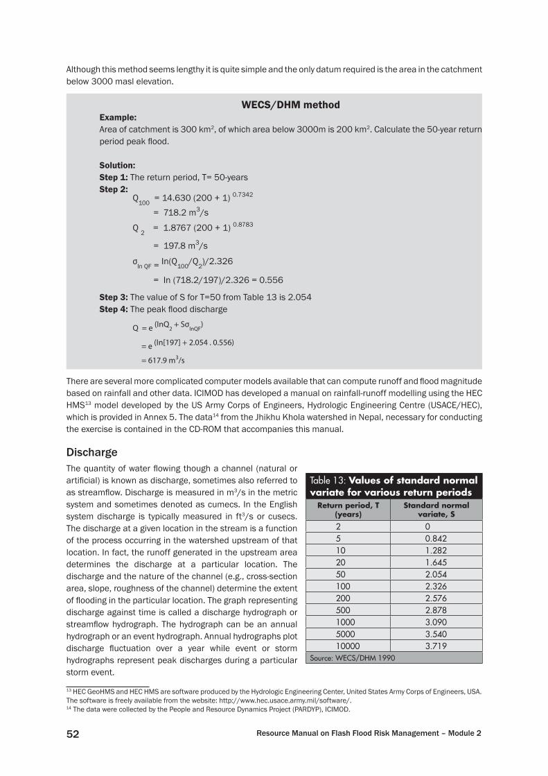
Resource Manual on Flash Flood Risk Management – Module 252
Although this method seems lengthy it is quite simple and the only datum required is the area in the catchment below 3000 masl elevation.
WECS/DHM methodExample:Area of catchment is 300 km2, of which area below 3000m is 200 km2. Calculate the 50-year return period peak fl ood.
Solution:Step 1: The return period, T= 50-yearsStep 2:
Q100
= 14.630 (200 + 1) 0.7342
= 718.2 m3/s
Q 2
= 1.8767 (200 + 1) 0.8783
= 197.8 m3/s
σIn QF = In(Q
100/Q
2)/2.326
= In (718.2/197)/2.326 = 0.556
Step 3: The value of S for T=50 from Table 13 is 2.054Step 4: The peak fl ood discharge
Q = e (InQ2 + Sσ
InQF)
= e (In[197] + 2.054 . 0.556)
= 617.9 m3/s
There are several more complicated computer models available that can compute runoff and fl ood magnitude based on rainfall and other data. ICIMOD has developed a manual on rainfall-runoff modelling using the HEC HMS13 model developed by the US Army Corps of Engineers, Hydrologic Engineering Centre (USACE/HEC), which is provided in Annex 5. The data14 from the Jhikhu Khola watershed in Nepal, necessary for conducting the exercise is contained in the CD-ROM that accompanies this manual.
DischargeThe quantity of water fl owing though a channel (natural or artifi cial) is known as discharge, sometimes also referred to as streamfl ow. Discharge is measured in m3/s in the metric system and sometimes denoted as cumecs. In the English system discharge is typically measured in ft3/s or cusecs. The discharge at a given location in the stream is a function of the process occurring in the watershed upstream of that location. In fact, the runoff generated in the upstream area determines the discharge at a particular location. The discharge and the nature of the channel (e.g., cross-section area, slope, roughness of the channel) determine the extent of fl ooding in the particular location. The graph representing discharge against time is called a discharge hydrograph or streamfl ow hydrograph. The hydrograph can be an annual hydrograph or an event hydrograph. Annual hydrographs plot discharge fl uctuation over a year while event or storm hydrographs represent peak discharges during a particular storm event.
13 HEC GeoHMS and HEC HMS are software produced by the Hydrologic Engineering Center, United States Army Corps of Engineers, USA. The software is freely available from the website: http://www.hec.usace.army.mil/software/.14 The data were collected by the People and Resource Dynamics Project (PARDYP), ICIMOD.
Table 13: Values of standard normal variate for various return periods
Return period, T (years)
Standard normal variate, S
2 05 0.84210 1.28220 1.64550 2.054100 2.326200 2.576500 2.8781000 3.0905000 3.54010000 3.719
Source: WECS/DHM 1990

53Chapter 6: Hazard-specifi c Flash Flood Management Measures
Rating curveAlthough a hydrograph gives continuous discharge values, continuous measurement of discharge in the river is rarely carried out. Generally, the water level at the gauging site is recorded on a continuous basis using an automatic recorder or manual gauge reading. The water-level data are converted to discharge using a discharge: water level relationship known as a rating curve. A rating curve is developed for each gauging site using a set of discharge measurements (Figure 40).
Measurement of discharge There are many different methods for measuring discharge.
Velocity area methodThe velocity area method is the most common method used. The cross-section of the river is divided into several vertical sections and the velocity of the water fl ow is measured at fi xed depths in each section. A current meter is used to measure velocity. Generally, the velocity is measured at 0.2 and 0.8 of the river’s depth. The velocity can be measured from a cable car, or if the depth is low, a wading technique can be used (Figure 41). The average of the two velocity measurements gives the average velocity of that section. The velocity of each section is multiplied by the area of the section, and the products for each section are summed to derive the discharge of the whole cross-section.
nQ = ∑ A
i • V
i
i=1
Where Q = discharge A = area of section i V = velocity of section i
Float methodThe velocity can also be calculated by a simpler method if the depth is shallow and high accuracy is not required. Two markers are fi xed on the stream bank at the same distance upstream and downstream from the cross-section where discharge measurement is being conducted. The distance between the markers is measured and the cross-section area of the stream at the point of interest is measured. A fl oating object such as a cork or wooden block is released at the centre of the stream. The time when the fl oat crosses the fi rst and the second marker is noted.
Measured data
Rating curve
Wat
er le
vel (
m)
Discharge (m3/s)
Figure 40: Rating curve
a. b.
c.
Figure 41: a. Current meter; b. velocity measurement from a cable car; and c. velocity measurement using the wading technique
Sou
rce:
htt
p://
wat
erkn
owle
dge.
colo
stat
e.ed
u/q.
htm
(Acc
esse
d M
ay 2
007
)

Resource Manual on Flash Flood Risk Management – Module 254
The velocity of the river is given by:
dv = T2
– T1
Where T1 and T2 are the times recorded at markers 1 and 2, respectively, and d is the distance between the two markers.
Such fl oat measurements are conducted several times and the mean velocity, Vm is calculated.
The discharge at the cross-section of interest is given by:
Q = A . Vm
Where A is the cross-section area.
Dilution methodThis method is particularly appropriate for mountainous streams where due to high gradient the turbulence is high and current-meter measurements are not possible. A tracer of known concentration is put in the upstream end of the specifi ed reach and its concentration is monitored in the downstream reach. The distance should be adequate to ensure thorough mixing of the tracer in the water and there should not be an inlet, outfl ow, or stagnant water zone within the reach. The tracer can be common salt or a fl uorescent dye, which is not readily adsorbed by the bed materials of the stream and the suspended sediment. The tracer can be injected into the stream instantaneously or in a continuous manner at a constant rate. For continuous injection a special apparatus called a Mariotte bottle is used (Figure 42a). The concentration at the downstream end is determined by collecting a water sample (Figure 42b) and analysing it using appropriate techniques. If a salt tracer is used, a conductivity meter is used to derive the concentration, while for a dye tracer, a fl uorimeter is used (Figure 42c). The discharge Q can be calculated using following equation:
C1 – C
2Q = q •
C
2 – C
0
Where q is the injection rate of the tracer and C1, C2 and C0 are the concentration of the tracer during injection, at the downstream end (sampling point), and in the background concentration of the stream water respectively. The method is described in detail in Merz (2007).
Slope area methodThis method is particularly suitable for post-fl ood investigations to estimate the peak discharge of a fl ash fl ood after the fl ood has passed. This is an indirect method of obtaining discharge in streams, in which velocity is not measured but instead calculated using the Manning uniform fl ow equation. To compute velocity, the area, the wetted perimeter, the channel slope, and the roughness of the reach where the discharge is going to be determined must be known (Figure 43). The area, the perimeter, and the slope are measured and the roughness coeffi cient is estimated as accurately as possible. The Manning equation15 is:
21
32
1SRnV ••=
Where, n is the Manning coeffi cient, R is the hydraulic radius, and S is the longitudinal slope (see Figure 43).
15 This form of the Manning equation is only valid for metric units.

55Chapter 6: Hazard-specifi c Flash Flood Management Measures
a.
b.
c.
Figure 42: Discharge measurement using the dilution method: a. dye tracer injection using a Mariotte bottle; b. sample collection; and c. laboratory analysis of tracer concentration

Resource Manual on Flash Flood Risk Management – Module 256
The steps for estimating discharge using the slope area method are as follows:Step 1: A straight river with as uniform a slope, cross-section, and roughness as possible is selected.Step 2: A detailed survey of the river reach is conducted and the Manning roughness coeffi cient, n, for the
river reach estimated. The Manning coeffi cient can be taken from Table 14. The highest fl ood mark should also be recorded.
Step 3: The survey data are used to calculate the fl ow area A and determine the wetted perimeter P. The longitudinal slope also needs to be taken into account. The hydraulic radius, R, is calculated using:
PA
R =
The values thus obtained are used to calculate the fl ow velocity during the fl ash fl ood using the Manning equation. Then the discharge, Q, is calculated from Q = A x V.
Flood routingFlood routing is a procedure to determine the time and magnitude of fl ow at a point on a water course from a known or assumed fl ood at one or more points upstream. Methods to determine runoff from a catchment due to a rainfall event are described above. The runoff will produce a certain level of fl ooding at the outlet of the catchment. It is also necessary to understand the impact of such a fl ood at the locations of different communities and settlements downstream of the catchment outlet. Flood routing can provide such information; it is a highly technical procedure and several computer software programs are available to conduct complicated fl ood routing. Here we describe a simple method with examples.
The basic principle of fl ood routing is the continuity of fl ow expressed by the continuity equation. There are several methods of fl ood routing including modifi ed plus, kinematic wave, Muskingum, Muskingum-Cunge, and dynamic (Chow et al. 1988). Here we limit our discussion to the Muskingum method, a commonly used hydrological fl ood routing method that models the storage volume of fl ooding in a stream channel by a combination of wedge and prism storage (Figure 44).
Flood level
Wetted perimeter = P
Nature of the bed = n
Slope = S
Flow area = A
Figure 43: Slope area method

57Chapter 6: Hazard-specifi c Flash Flood Management Measures
Source: USGS (http://wwwrcamnl.wr.usgs.gov/sws/fi eldmethods/indirects/nvalues/ Accessed May 2007)
Table 14: Table for estimation of Manning’s coeffi cient, n

Resource Manual on Flash Flood Risk Management – Module 258
During the advance of a fl ood wave, infl ow exceeds outfl ow, producing a wedge of storage. During the recession of a fl ood, outfl ow exceeds infl ow, producing a negative wedge shape. In addition, there is a prism of storage which is formed by a volume of constant cross-section along the length of a prismatic channel.
The prism storage Sp = K Q
Where K is the proportionality coeffi cient and Q is the constant discharge equal to the outfl ow at the beginning.
The wedge storage Sw= K (I - Q) X
Where I is the total infl ow due to fl ood and X is a weighting factor with a range of 0 ≤ X ≤ 0.5.The total storage S = Sp + Sw = KQ + K (I –Q) X = K[X I + (1-X) Q].
The storage at times j and j +1 can be written as: Sj = K [X Ij + (1 - X) Qj] and
Sj+1 = K [X Ij+1 + (1 - X) Qj+1]
The difference in storage between these times is Sj+1 – Sj = K{[X Ij+1 + (1 - X) Qj+1] – [X Ij + (1 – X) Qj]}.
The change in storage is also given by the following equation:
S
j+1 – S
j =
(Ij + I
j+1) (Q
j + Q
j+1)
2 2∆t – ∆t
Wedge Storage= K X (I - Q)
Prism Storage= K Q
i - Q
Q
Q
Figure 44: Prism and wedge storage in a channel reach

59Chapter 6: Hazard-specifi c Flash Flood Management Measures
Combining the two equations we get the routing equation of the Muskingum method:
Q
j+1 = C
1Ij+1
+ C2Ij + C
3Q
j
Where
tXK
KXtC
∆+−
−∆=
)1(2
21
tXK
KXtC
∆+−
+∆=
)1(2
22
tXK
tXKC
∆+−
∆−−=
)1(2
)1(23
Note that C1+C2+C3 = 1.
In the Muskingum method, K and X are determined graphically from the hydrograph, while in the Musking-Cunge method they can be determined using the following equations:
kcx
K∆
= )1(21
0
max
xcBS
QX
k ∆−=and
Where Ck is celerity, and B is the width of the water surface.
The method becomes much clearer from the following exercise:
Exercise on fl ood routing
Example:The hydrograph at the upstream end of a river is given in the following table. The reach of interest is 18 km long. Using a subreach length Δx of 6km, determine the hydrograph at the end of the reach using the Muskingum-Cunge method. Assume ck = 2m/s, B = 25.3m, S0 = 0.001m, and no lateral fl ow.
Time (hour) 0 1 2 3 4 5 6 7 8 9 10 11 12
Flow (m3/s) 10 12 18 28.5 50 78 107 134.5 147 150 146 129 105
Time (hr) 13 14 15 16 17 18 19 20 21 22 23 24
Flow (m3/s) 78 59 45 33 24 17 12 10 10 10 10 10
Solution:Step 1: Determine K
sec3000
26000 ==∆=
kcxK
Step 2: Determine X
253.0)
)6000) (2) (001.0) (3.25(150
1(21)1(
21
0
max =−=∆
−=xcBS
QX
k
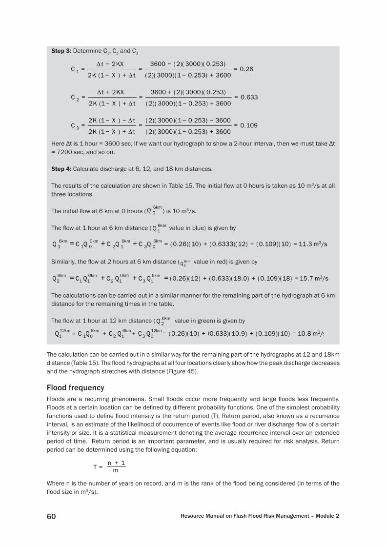
Resource Manual on Flash Flood Risk Management – Module 260
Step 3: Determine C1, C2 and C3
26.03600)253.01)(3000)(2(
)253.0)(3000)(2(3600
)1(2
21 =
+−
−=
∆+−
−∆=
tXK
KXtC
633.03600)253.01)(3000)(2(
)253.0)(3000)(2(3600
)1(2
22 =
+−
+=
∆+−
+∆=
tXK
KXtC
109.03600)253.01)(3000)(2(
3600)253.01)(3000)(2(
)1(2
)1(23 =
+−
−−=
∆+−
∆−−=
tXK
tXKC
Here Δt is 1 hour = 3600 sec. If we want our hydrograph to show a 2-hour interval, then we must take Δt = 7200 sec, and so on.
Step 4: Calculate discharge at 6, 12, and 18 km distances.
The results of the calculation are shown in Table 15. The initial fl ow at 0 hours is taken as 10 m3/s at all three locations.
The initial fl ow at 6 km at 0 hours (kmQ 6
0 ) is 10 m3/s.
The fl ow at 1 hour at 6 km distance ( kmQ 61 value in blue) is given by
3 m3/s.11)10)(109.0()12)(6333.0()10)(26.0(603
012
001
61 =++=++= kmkmkmkm QCQCQCQ
Similarly, the fl ow at 2 hours at 6 km distance ( kmQ 62
value in red) is given by
7 m3/s.15)18)(109.0()0.18)(633.0()12)(26.0(613
012
011
62 =++=++= kmkmkmkm QCQCQCQ
The calculations can be carried out in a similar manner for the remaining part of the hydrograph at 6 km distance for the remaining times in the table.
The fl ow at 1 hour at 12 km distance ( kmQ 62 value in green) is given by
8 m3/s.10)10)(109.0()9.10)(633.0)10)(26.0( (1203
612
601
121 =++=++=
kmkmkmkm QCQCQCQ
The calculation can be carried out in a similar way for the remaining part of the hydrographs at 12 and 18km distance (Table 15). The fl ood hydrographs at all four locations clearly show how the peak discharge decreases and the hydrograph stretches with distance (Figure 45).
Flood frequencyFloods are a recurring phenomena. Small fl oods occur more frequently and large fl oods less frequently. Floods at a certain location can be defi ned by different probability functions. One of the simplest probability functions used to defi ne fl ood intensity is the return period (T). Return period, also known as a recurrence interval, is an estimate of the likelihood of occurrence of events like fl ood or river discharge fl ow of a certain intensity or size. It is a statistical measurement denoting the average recurrence interval over an extended period of time. Return period is an important parameter, and is usually required for risk analysis. Return period can be determined using the following equation:
m
nT
1+=
Where n is the number of years on record, and m is the rank of the fl ood being considered (in terms of the fl ood size in m³/s).

61Chapter 6: Hazard-specifi c Flash Flood Management Measures
Table 15: Calculation of fl ow values at different times and locations
Flow (m3/s)
Time (hr) 0 km 6 km 12 km 18 km
0 10.0 10.0 10.0 10.0
1 12.0 11.3 10.8 10.5
2 18.0 15.7 14.1 12.9
3 28.5 24.4 21.1 18.4
4 50.0 41.7 35.1 29.7
5 78.0 66.9 57.0 48.5
6 107.0 95.3 83.9 73.2
7 134.5 123.3 112.0 100.7
8 147.0 141.5 133.8 124.8
9 150.0 148.6 145.4 140.5
10 146.0 147.6 147.9 146.8
11 129.0 135.7 140.4 143.3
12 105.0 114.8 123.3 130.1
13 78.0 89.2 99.7 109.4
14 59.0 67.3 76.7 86.4
15 45.0 51.2 58.3 66.2
16 33.0 38.2 43.8 50.1
17 24.0 27.9 32.4 37.3
18 17.0 20.0 23.5 27.4
19 12.0 14.2 16.8 19.7
20 10.0 11.0 12.5 14.4
21 10.0 10.1 10.6 11.5
22 10.0 10.0 10.1 10.4
23 10.0 10.0 10.1 10.1
24 10.0 10.0 10.0 10.1
Figure 45: Hydrographs at different locations

Resource Manual on Flash Flood Risk Management – Module 262
Calculation of return period is explained by the following example based on the data given in Table 16.
Step 1: The discharge data is arranged in ascending order as in column 2 of Table 17.Step 2: Rank the discharge data as in column 3 of Table 17.Step 3: Determine the return periods from the equation given above.
Table 17: Calculation of return period
YearAnnual maximum 1-day fl ood
(x1000 m3/s)Rank of the fl ood Return Period
Q m T
1952 3.68 1 31.00
1965 4.39 2 15.50
1943 4.82 3 10.33
1957 5.81 4 7.75
1964 6.09 5 6.20
1948 6.23 6 5.17
1951 6.48 7 4.43
1960 7.22 8 3.88
1947 7.28 9 3.44
1963 7.65 10 3.10
1940 8.44 11 2.82
1955 8.50 12 2.58
1950 9.68 13 2.38
1956 9.72 14 2.21
1966 10.34 15 2.07
1953 11.43 16 1.94
1946 12.45 17 1.82
1967 12.88 18 1.72
1941 14.00 19 1.63
1939 14.57 20 1.55
1949 18.30 21 1.48
1962 18.70 22 1.41
1958 19.65 23 1.35
1961 20.86 24 1.29
1954 21.24 25 1.24
1942 22.62 26 1.19
1945 24.20 27 1.15
1944 29.30 28 1.11
1959 37.30 29 1.07
1968 42.50 30 1.03
30n27.426Q ==Σ
Table16: Annual maximum one-day fl ood dataYear 1939 1940 1941 1942 1943 1944 1945 1946 1947 1948 1949 1950 1951 1952 1953
Discharge (m3/s) 14.57 8.44 14.00 22.62 4.82 29.30 24.20 12.45 7.28 6.23 18.30 9.68 6.48 3.68 11.43
Year 1954 1955 1956 1957 1958 1959 1960 1961 1962 1963 1964 1965 1966 1967 1968
discharge (m3/s) 21.24 8.50 9.72 5.81 19.65 37.30 7.22 20.86 18.70 7.65 6.09 4.39 10.34 12.88 42.50

63Chapter 6: Hazard-specifi c Flash Flood Management Measures
The return period is important in relating extreme discharge to average discharge. The return period has an inverse relationship with the probability (P) that the event will be exceeded in any one year. For example, a 10-year fl ood has a 0.1 or 10% chance of being exceeded in any one year and a 50-year fl ood has a 0.02 (2%) chance of being exceeded in any one year.
It is commonly assumed that a 10-year fl ood will occur, on average, once every 10 years and that a 100-year fl ood is so large that we expect it to occur only once every 100 years. While this may be statistically true over thousands of years, it is incorrect to think of the return period in this way. The term ‘return period’ is actually a misnomer. It does not necessarily mean that the design storm of a 10-year return period will return every 10 years. It could, in fact, never occur, or occur twice in a single year. It is still considered a 10-year storm.
Return period is useful for risk analysis (such as natural, inherent, or hydrological risk of failure). When dealing with structural design expectations, the return period is useful in calculating the risk to the structure with respect to a given storm return period given the expected design life. The equation for assessing this risk can be expressed as
nT
n xXPT
R ))(1(1)11(1_
≥−−=−−=
Where )(
1TxXP
T≥=
expresses the probability of the occurrence for the hydrological event in question, and n is the expected life of the structure.
6.2 Landslide Dam Outburst FloodUnderstanding the processLandslides usually occur as secondary effects of heavy storms, earthquakes, and volcanic eruptions. Bedrock or soil (earth and organic matter debris) are the two classes of materials that compose landslides. A landslide may be classifi ed by its type of movement, as shown in Figure 46.
Falls: A fall is a mass of rock or other material that moves downward by falling or bouncing through the air. These are most common along steep road or railroad embankments, steep escarpments, or undercut cliffs (especially in coastal areas). Large individual boulders can cause signifi cant damage. Depending on the type of materials involved, it may be rockfall, earthfall, debris fall, and so on.
Topple: A topple occurs due to overturning forces that cause a rotation of the rock out of its original position. The rock section may have settled at a precarious angle, balancing itself on a pivotal point from which it tilts or rotates forward. A topple may not involve much movement, and does not necessarily trigger a rockfall or rock slide.
Slides: Slides result from shear failure (slippage) along one or several surfaces; the slide material may remain intact or break up. The two major types of slides are rotational and translational slides. Rotational slides occur on slopes of homogeneous clay of shale and soil slopes, while translational slides are mass movements on a more or less plane surface.
Lateral spreads: A lateral spread occurs when large blocks of soil spread out horizontally after fracturing off the original base. Lateral spreads generally occur on gentle slopes of less than 6%, and typically spread 3m to 5m, but may move from 30m to 50m where conditions are favourable. Lateral spreads usually break up internally and form numerous fi ssures and scarps. The process can be caused by liquefaction whereby saturated, loose sand or silt assumes a liquefi ed state. This is usually triggered by ground shaking, as with an earthquake. During the 1964 Alaskan earthquake, more than 200 bridges were damaged or destroyed by lateral spreading of fl ood plain deposits near river channels.

Resource Manual on Flash Flood Risk Management – Module 264
Flows: Flows move like a viscous fl uid, sometimes very rapidly, and can cover several miles. Water is not essential for fl ows to occur, although most fl ows form after periods of heavy rainfall. A mudfl ow contains at least 50% sand, silt, and clay particles. A lahar is a mudfl ow that originates on the slope of a volcano and may be triggered by rainfall, sudden melting of snow or glaciers, or water fl owing from crater lakes. A debris fl ow is a slurry of soils, rocks, and organic matter combined with air and water. Debris fl ows usually occur on steep gullies. Very slow, almost imperceptible, fl ow of soil and bedrock is called creep. Flows can be creep, debris fl ow, debris avalanche, earth fl ows, or mud fl ows.
Where landslides can dam a riverBoth natural and anthropogenic factors can initiate dam-forming landslides. The most important natural processes in initiating dam-forming landslides are excessive precipitation (rainfall and snowmelt) and earthquakes (Figure 47).
Figure 47 shows that globally about 50% of dam-forming landslides are caused by rainstorms and snowmelt, about 40% by earthquakes, and only 10% by other factors. As volcanic eruptions are rare in the HKH region, the percentage of landslides causing dam formation due to rainfall, snowmelt, and earthquakes is higher.
Landslide dams form most frequently where narrow steep valleys are bordered by high rugged mountains (Table 18). This setting is common in geologically active areas where earthquakes and glacially steepened slopes occur, which is typical of the HKH region. These areas contain abundant landslide source materials, such as sheared and fractured bed materials, and experience triggering mechanisms which initiate landslides. Steep, narrow valleys require a relatively small volume of material to form dams; thus, even small mass movements present a potential for formation of landslide dams. Such dams are much less common in broad, open valleys. Most landslide dams are caused by falls, slides, and fl ows. Large landslide dams are often caused by complex landslides that start as slumps of slides and transform into rock or debris avalanches.
Modes of failure of landslide damsA landslide dam in its natural state differs from a constructed dam in that it is made up of a heterogeneous mass of unconsolidated or poorly consolidated material and has no proper drainage system to prevent piping
Talus
a. Fall b. Topple c. Slide
d. Spread
Original Position
Moving Mass
e. Flow
Figure 46: Types of landslides
Sou
rce:
Deo
ja e
t al
. 19
91

65Chapter 6: Hazard-specifi c Flash Flood Management Measures
and control pore pressures. It also has no channelised spillway or other protected outlets; as a result, landslide dams commonly fail by overtopping, followed by breaching following erosion by the overfl ow water. In most documented cases, the breach has resulted from fl uvial erosion of the landslide material, with headcutting originating at the toe of the dam and progressively moving upstream to the lake. When the headcut reaches the lake, breaching occurs. The breach commonly does not erode down to the original river level as many landslide dams contain some coarse material that armours the streambed locally. Smaller lakes can thus remain after dam failure.
Because landslide dams do not undergo systematic compaction, signifi cant porosity and seepage through the dam can cause piping, which can lead to internal structural failure, although failure due to piping and seepage are quite rare compared to failure due to overtopping (Figure 48). In some cases piping and undermining of the dam can cause partial collapse of the dam, followed by overtopping and breaching.
A landslide dam with steep upstream and downstream faces and with high pore-water pressure is susceptible to slope failure. If the dam has a narrow cross-section or the slope failure is progressive, the crest may fail, leading to overtopping and breaching. Nearly all faces of landslide dams are at the angle of repose of the
0
10
20
30
40
50
60
Rains to rm and s no wm elt
E arthq uakes V o lc anic erup t io ns O ther
% o
f all
events
Sou
rce:
Bas
ed o
n C
osta
and
Sch
uste
r 1
98
8
Figure 47: Causes of landslides that have formed dams
Table 18: Factors causing dam forming landslidesNatural Anthropogenic
High relief Deforestation
Undercutting of river banks Improper landuse
Weak geology - agriculture on steep slopes
High weathering - irrigation of steep slopes
Intensive rainfall - overgrazing
High snowmelt - quarrying
Poor sub-surface drainage Construction activities
Seismic activities

Resource Manual on Flash Flood Risk Management – Module 266
material or less; however, because they are formed dynamically, slope failures are rare. A special type of slope failure involves lateral erosion of the dam by a stream or river.
0
10
20
30
40
50
60
70
80
O v erto p p ing P ip ing S lo p e f ailure P hy s ic ally c o ntro lled
(d id not f a il)
% o
f all e
vent
s
Figure 48: Modes of failure of landslide dams
Sou
rce:
Bas
ed o
n C
osta
and
Sch
uste
r 1
98
8
Main triggers of landslides
Rainfall-induced landslidesRainfall is an important landslide trigger. There is a direct correlation between the amount of rainfall and the incidence of landslides.
Cumulative rainfall between 50-100 mm in one day and daily rainfall exceeding 50 mm can cause small-scale and shallow debris landslides.
Cumulative two-day rainfall of about 150 mm, and daily rainfall of about 100 mm, have a tendency to increase the number of landslides.
Cumulative two-day rainfall exceeding 250 mm, or an average intensity of more than 8 mm per hour in one day, rapidly increases the number of large landslides.
Earthquake-induced landslidesEarthquakes can cause many large-scale, dam-forming landslides. Seismic accelerations, duration of shock, focal depth, and angle and approach of seismic waves all play a role in inducing landslides, but environmental factors such as geology and landforms play the most important role. This is why small earthquakes can sometimes induce more landslides than large earthquakes.
The type of slope and the slope angle have a great infl uence upon landslides. Landslides rarely occur on slopes less than 25°. The large majority of landslides occur on slopes with angles ranging from 30° to 50°.

67Chapter 6: Hazard-specifi c Flash Flood Management Measures
Longevity of landslide damsLandslide-dammed lakes may last for several minutes or several thousands of years, depending on many factors, including volume, size, shape, sorting of blockage material, rates of seepage, and so on. External factors can also determine the longevity of landslide dams. For example, high stream infl ow, intensive rainfall, or rockfall into the lake can cause rapid collapse of the dam.
There is very little time for action in the case of landslide dam formation. About 40% of landslide dams fail within a week of formation, and 80% fail within 6 months (Figure 49). It is clear that in the majority of cases there is not much time to mitigate the effects of dam failure unless a good local disaster management plan is in place.
Three factors govern the longevity of landslide dams: 1) rate of infl ow to the impoundment; 2) size and shape of the dam; and 3) geophysical characteristics of the dam. The life of a dam can be shortened signifi cantly due to the external factors mentioned above. The infl ow rate is generally proportional to the upstream catchment area and is signifi cantly greater during monsoon seasons. Landslide dams of predominantly soft, low-density, fi ne-grained, or easily liquifi ed sediment lack resistance to erosion and are more susceptible to failure. Landslide dams comprised of larger and cohesive material are more resistant to failure. Poorly sorted materials with d15/d85 ratios greater than 5 are susceptible to internal erosion by piping (Sherard 1979).
Measures to minimise the risk of LDOFControl measures, such as the construction of spillways to drain the ponded water, have been attempted in various places around the world. Sometimes these measures have been successful in preventing an LDOF, in others overtopping has occurred before satisfactory control measures could be constructed. In some cases, the attempts themselves triggered fl oods that caused large-scale casualities. Here we focus on non-structural measures to mitigate LDOFs.
Landslide hazard assessmentThe fi rst approach in LDOF mitigation is to identify places where the hazard can occur. This can be accomplished by preparing a landslide hazard map. If a landslide can occur in a narrow valley close to a stream, it could potentially cause a lake-forming dam. Additional analysis may provide an estimate of the volume of the dam, which together with the stream infl ow rate can give an indication of the rate of lake level rise.
Hazard and risk mapping is done using 1) a simple qualitative method, which is based on experience and uses an applied geomorphic approach to determine parameters and their weightings, and scores and overlays of parameter maps for pre-feasibility level; 2) a statistical method score for the different parameters determined based on bi-variate and multivariate statistical analysis; 3) a deterministic method based on the properties of materials; and 4) social mapping using information derived from discussions with local people based on their experiences and feelings.
0
20
40
60
80
100
0 100 200 300 400
Age of dam at failure (days)
% o
f dam
s fa
ilin
g b
elo
w
the
ind
icat
ed a
ge
27% failures < 1 day
41% failures < 1 week
50 % failures < 10 days
56 % failures < 1 month
80 % failures < 6 months86 % failures < 1 years
Figure 49: Length of time before failure of landslide dams (based on 73 case studies)
Sou
rce:
Bas
ed o
n C
osta
and
Sch
uste
r 1
98
8

Resource Manual on Flash Flood Risk Management – Module 268
The hazard may be classifi ed as relative (assigning ratings to different factors contributing to hazard), absolute (deterministically derived, e.g., factor of safety), or monitored (actual measurement of effects, e.g., deformation along roads, rocks, and so on).
Relative hazard assessment generally follows these stepsdetermination of different factors contributing to slope instability ●
development of a rating scheme and scores for hazard probability ●
identifi cation of elements at risk and their quantifi cation ●
development of a rating scheme and scores for damage potential ●
construction of a hazard and risk matrix ●
mapping of hazard and risk ●
Estimation of downstream fl oodingInformed estimates about the magnitude of a potential fl ood are necessary in order to implement mitigation measures in areas downstream of the landslide-dammed lake. This can be done through techniques involving varying degrees of complexity. As, in most cases, the time between the dam formation and outburst is so short, a detailed analysis may not be possible and estimates will have to rely on simple techniques. Costa and Schuster (1988) suggested the following regression equation to estimate peak discharge of a LDOF:
Q = 0.0158Pe0.41
Where Q is peak discharge in cubic metres per second, and Pe is the potential energy in joules.
Pe is the potential energy of the lake water behind the dam prior to failure and can be calculated using the following equation:
Pe = Hd x V x γ
Where Hd is the height of the dam in metres, V is the volume of the stored water, and γ is the specifi c weight of water (9810 Newton/m3).
Mizuyama et al. (2006) suggest the following equation for calculating peak discharge:
( )
6
33
1010
tan
542.0Bq
q
ghQ
in
in
⋅⋅
⎪⎭
⎪⎬⎫
⎪⎩
⎪⎨⎧
⋅⋅
=
θ
0.5
0.565
Where Q is the peak discharge in m3/s; qin the infl ow into the lake in cm3/s; g the gravitation acceleration (about 9.8 m/s2); h the dam height in metres; and θ the stream-bed gradient.
Figure 50 shows a schematic diagram of the input parameters and an example of calculating peak outfl ow is given below. The two methods give entirely different results as they include different parameters, the second method including more parameters than the fi rst.
Sophisticated computer models are available to estimate the peak outfl ow of the LDOF and to route the fl ood along the river reach downstream of the lake. This will give the area and level of fl ooding, and can help in making decisions regarding relocating people or implementing structural mitigation measures.

69Chapter 6: Hazard-specifi c Flash Flood Management Measures
Estimation of past fl oodsEstimation of past fl oods provides an idea of the magnitude of fl oods that are likely to affect a location. The slope-area method for estimating the magnitude of past fl oods is described above. Paleohydraulic reconstruction techniques can also provide estimates of past fl oods. These techniques reconstruct the velocity of the fl ow, depth, and width of the channel during the fl ood based on the size of boulders deposited by the fl ood. Details are given in Costa (1983). These estimates provide a basis for identifying the magnitude of a past fl ood and for assessing potential future hazard and risk.
h
qin
a.
b.
B
q in
Θ
Figure 50: A schematic diagram showing the parameters used in calculating peak outfl ow discharge: a. isometric view; and b. cross-section.

Resource Manual on Flash Flood Risk Management – Module 270
The following steps are used to reconstruct the fl ood magnitude:
Step 1: Velocity calculationSeveral equations have been developed for calculating the velocity of a past fl ood based on the size of boulders deposited. Here we present some of the common ones.
(i) Mavis and Laushey (1949)
( ) 2
194
15.0 −= gb SdV
Where Vb is the bed velocity of fl ow in ft/s, d is the boulder diameter in mm, and Sg is the specifi c gravity of the boulder.
The mean velocity is calculated as
VV b3
1_=
Example of LDOF peak outfl ow calculation
Let us assume the following input parametersH = 50m; B = 200m; θ = 5°
First we derive the volume of the lake:V = ½ h x B x L
Where l = h/tan 5° = 50/0.087 = 574m
V = 0.5 x 50m x 200m x 574m = 2,870,000 m3
Pe = Hd x V x γ, Pe = 50 x 2,870,000 x 9810 = 14 x 1011
Substituting into equation Q = 0.0158 pe0.41
Q = 0.0158 x (14 x 1011) 0.41 = 1511.9 m3/s
Now let us apply equation by Mizuyama to calculate the peak discharge.
Let us assume the infl ow qin is 50 m3/s or 50 x 106 cm3/s
( )6
6565.0
36
5.03
10
200)1050(10
)1050(tan5
5081.9542.0
⋅⋅⋅
⎪⎭
⎪⎬⎫
⎪⎩
⎪⎨⎧
⋅⋅⋅
⋅=Q
100001017.4374433
36.1107542.0
565.0
3 ⋅⎭⎬⎫
⎩⎨⎧ ⋅=
= 0.542 x 0.46 x 10000
= 2494 m3/s

71Chapter 6: Hazard-specifi c Flash Flood Management Measures
(ii) Strand (1977)
21
51.0 dVb=
Where Vb is velocity of fl ow in ft/s and d is the boulder diameter in mm. The mean velocity of fl ow is derived in the same way as for Mavis and Laushey (1949).
(iii) Williams (1983)
5.0
_065.0 dV =
Where V_
is the mean velocity of fl ow (m/s) and d is the diameter of the boulder in mm.
Step 2: Depth CalculationThe next step is to calculate the mean depth of the fl ow. Again several methods are available for calculating the mean depth.
(i) Manning’s equation
5.1__)(
SnVD =
√
Where D_
is mean depth, n is the roughness
coeffi cient, and S the slope.
(ii) Costa (1983)
In this method, a nomogram developed by Costa (1983; Figure 51) is used to derive the mean depth.
(iii) Sheild (1936)
SD fd S /)(.
_γγθ −=
Where θ is dimensionless shear stress (use 0.02), γf
= 1070 kg/m3, and γs= 2700
kg/m3.
(iv) Williams (1983)
SfD γτ/
_=
d 0.117.0=τ
Where τ is shear stress (N/m2), d is diameter of boulder (mm), and γ is the specifi c weight of water.
Step 3: Width calculationThe width is determined using an iterative method. A straight reach for cross-section (neither expanding nor contracting) is selected. The site should not be abnormally wide, narrow, steep, or fl at. At least one, and preferably both, valley walls should be bedrock. The site should be close to the depositional site. Select at least two cross-sections spaced about one valley-width apart. No major tributaries should enter the main channel between the cross-sections.
10
5
1.0
0.5
0.150 100 500 1000 5,000 10,000
0.005
0.01
0.02
0.05
0.10
d (mm)
D (m
)
Figure 51: Graph to predict average depth (D_
) of past fl ood from boulder size (d) and channel slope. The numbers beside the lines indicate the channel slopes.
Sou
rce:
Fro
m C
osta
19
83

Resource Manual on Flash Flood Risk Management – Module 272
Once the cross-sections have been plotted, draw a line to represent the estimated top width of the cross-section (Figure 52). Using a planimeter or a digitiser, calculate the area of the cross-section and divide it by the top width of the cross-section. If the value deviates from the estimated depth from Step 2, draw a new top-width line and repeat the process until the two values agree. Now, calculate the cross-sectional area ‘A’ for the fi nal top-width.
Step 4: Calculation of dischargeKnowing the average velocity from Step 1 and the cross-sectional area from Steps 2 and 3, a single discrete estimate of fl ood discharge (Q) can be made using the following equation:
AVQ .
_=
Land use regulationThe increasing hazard and risk of LDOFs are a result of unregulated use of land and investment in fl ood-prone areas for infrastructure development such as buildings and roads. Public buildings such as schools are being constructed even on small islands between river distributaries, and houses are encroaching on natural river channels. Figures 53 and 54 provide evidence of such practices. In this context, the most effective way to mitigate LDOFs is to avoid activities that can cause landslides, particularly in narrow valleys where landslides can result in lake-forming dams. In such areas, development activities should be located on stable ground and landslide-susceptible areas should be used for open space or for low-intensity activities such as parkland or grazing. Land use controls can prevent hazardous areas from being used for settlements or as sites for important structures. The controls may also involve relocation away from the hazardous area, particularly if alternative sites exist. Restrictions may be placed on the type and amount of building that may take place in high-risk areas. Activities that might activate a landslide should be restricted. Where the need for land is critical, expensive engineering solutions for stabilisation may be justifi ed. Building codes and design standards are also necessary.
Financial measuresGovernments may assume responsibility for the cost of repairing damage from LDOFs as well as efforts to prevent them. Insurance programmes may reduce losses from LDOF by spreading the expenses over a larger base and including standards for site selection and construction techniques. Financial measures may be used to relocate people/activities from a landslide-prone area.
A
W
0
1
2
3
4
0 5 1 0 1 5 2 0 2 5 3 0 3 5 4 0
De
pth
(m
)
D istance (m)Figure 52: Top-width (W) and cross-section area (A) for calculation of depth by the iterative method

73
N.R
. Kha
nal,
TU, N
epal
Figure 53: Damage resulting from the 1998 LDOF in Syangja, central Nepal

74
Early warning systemsEarly warning systems (EWSs) can be an effective measure to mitigate the impacts of LDOFs, particularly in saving life and property. Depending on the situation, a variety of early warning systems can be implemented. As the lifetime of landslide dams is often quite short, a sophisticated system may not be possible. In many cases the best option is to implement a community-based EWS. This may consist of placing people at strategic locations starting from the dam site to the distance downstream up to which the LDOF can have an impact. Each location should have visual contact with the person just upstream and downstream. EWSs as part of a monitoring, warning, and response system (MWRS) have been described in Chapter 5.
6.3 Glacial Lake Outburst FloodUnderstanding the processGlaciers A glacier is a large fl owing ice mass. The fl ow is an essential property in defi ning a glacier. Usually a glacier develops under conditions of low temperature caused by cold climate, although this in itself is not suffi cient to create a glacier. An area in which the total depositing mass of snow exceeds the total mass of snow melting during a year is defi ned as an accumulation area. Thus, snow layers are piled up year after year because the annual net mass balance is positive. As a result of the overburden pressure due to weight, compression occurs in the deeper snow layers, and the density of the snow layers increases. Snow becomes impermeable to air a critical density of approximately 0.83 g/cm3. The impermeable snow is called ice. Ice has a density ranging from 0.83 to a pure ice density of 0.917 g/cm3. Snow has a density range from 0.01 g/cm3 for fresh layers just after snowfall to ice at a density of 0.83 g/cm3. Perennial snow with high density is called ‘fi rn’. In the glacier, the snow changes to ice below a certain depth. When the thickness of ice exceeds a certain critical depth, the ice mass starts to fl ow down along the slope by plastic deformation and slides along the ground driven by its own weight. The lower the altitude, the warmer the climate. Below a critical altitude, the annual mass of deposited snow melts completely, the ‘end’ of the glacier. Here, snow disappears during the hot season and may not accumulate year after year. This area with a negative annual mass balance is
Figure 54: A school located on a small island between distributaries of the Bagmati River in Kavre District, Nepal
N.R
. Kha
nal,
TU, N
epal

75Chapter 6: Hazard-specifi c Flash Flood Management Measures
defi ned as the ablation area. A glacier is divided into two such areas, the accumulation area in the upper apart of the glacier and the ablation area in the lower part. The boundary line between them is defi ned as the equilibrium line, where the deposited snow mass is equal to the melting mass in a year. Ice mass in the accumulation area fl ows down into the ablation area and melts away. Such a dynamic mass circulation system is defi ned as a glacier. There are different types of glaciers, such as ice sheet, ice fi eld, ice cap, outlet glacier, valley glacier, mountain glacier, glacieret and snowfi eld, ice shelf, and rock glacier.
A glacier can change in size and shape due to the infl uence of climate change, advancing when the climate changes to a cool summer and heavy snowfall in winter and the monsoon season. As the glacier advances, it expands and the terminus shifts to a lower altitude. A glacier retreats when the climate changes to a warm summer and less snowfall. As the glacier retreats, it shrinks and the terminus climbs up to a higher altitude. Thus, climatic change results in a glacier shifting to another equilibrium size and shape.
Formation of glacial lakesThe formation and growth of glacial lakes is closely related to deglaciation. Shrinkage of glaciers is a widespread phenomenon in the HKH region at present, closely associated with climate change. The world has experienced many episodes of glacial and inter-glacial periods, during which glaciers advanced and retreated dramatically. A globally synchronous re-advance of glaciers occurred during the so-called ‘Little Ice Age’ (LIA), which prevailed from the middle of the 16th Century to the middle of the 19th Century16. The climate has gradually warmed since the end of the LIA, accompanied by the retreat of glaciers. Glacial retreat has accelerated in recent decades, generally attributed to human-induced increase of greenhouse gasses in the atmosphere and resultant overall warming. Valley glaciers generally contain supra-glacial ponds, which grow bigger and merge with a warming climate. This process is accelerated by rapid retreat of glaciers. As glaciers retreat, they leave a large void behind, and meltwater is trapped in the depression previously occupied by glacial ice thus forming a lake. Figure 55 shows the rapid growth of Tsho Rolpa lake in Nepal as an example.
1957-59
1960-68
1975-77
1979
1983-84
1988-90
1994
1997
2002
0.61 km2
0.62 km2
0.78 km2
0.80 km2
1.02 km2
1.16 km2
1.27 km2
1.39 km2
1.65 km2
1.76 km2
0 1 2 3 km
0.23 km2
1974
1972
Figure 55: Development of Tsho Rolpa glacial lake, Nepal
16 It was initially believed that the LIA was a global phenomenon, but recent studies question this. The beginning and end of the LIA is also a matter of debate among the scientifi c community.

Resource Manual on Flash Flood Risk Management – Module 276
Moraine damsGlacial lakes are retained by the moraine dams created by the glacier during its advance stage. Debris falling on glaciers due to weathering of surrounding slopes and materials collected from the bottom of the glacier, are dumped loosely at the end of glaciers forming a terminal or end moraine (1 in Figure 56) and at the side of the glaciers forming lateral moraines (2 in Figure 56). These moraine dams are structurally weak and unstable, and undergo constant changes due to slope failure, slumping, and so on. This process can be aggravated; there is a potential for catastrophic failure, causing a glacial lake outburst fl ood (GLOF).
Causes of failure of moraine damsA moraine dam may break as the result of the action of some external trigger or by self-destruction. A huge displacement wave generated by a rockslide or snow/ice avalanche from the glacier terminus (Figure 57, bottom) or hanging glaciers (5 in Figure 56) falling into the lake, may cause the water to overtop the moraines, creating a large breach and eventually causing dam failure (Ives 1986). Earthquakes may also trigger a dam break depending upon magnitude, location, and characteristics. Self-destruction is caused by the failure of the dam slope and seepage from the natural drainage network of the dam (Figure 57, top). Richardson and Reynolds (2000) analysed 26 GLOF events in the Himalayas in the 20th Century and concluded that a majority of the moraine dam failures were triggered by overtopping by a displacement wave caused by ice avalanches into the lake from hanging or calving glaciers (Figure 58).
Impacts of GLOFsA GLOF is characterised by a sudden release of a huge amount of lake water, which in turn rushes downstream along the stream channel in the form of dangerous fl ood waves. These fl ood waves are comprised of water mixed with morainic materials and can have devastating consequences for downstream riparian communities, hydropower stations, and other infrastructure. Rushing water erodes both banks of the river and causes landslides from the steep slopes along the river channel. A moraine-dammed lake outburst results in a greater rate of water release than an ice-dammed lake burst, as in the latter case the release of water occurs
1
2
2
3
4
55
6
6
6
4
Box 1
Box 2
Figure 56: Schematic view of a typical glacial lake in the Himalayas. 1) end moraine; 2) lateral moraine; 3) glacial lake; 4) glacier terminus; 5) hanging glacier; 6) talus slope (rock fall). Details of Boxes 1 and 2 are shown in Figure 57

77Chapter 6: Hazard-specifi c Flash Flood Management Measures
Figure 57: Detailed view of frontal part of the glacial lake, Box 1 in Figure 56 (top), and terminus of the parent glacier, Box 2 in Figure 56 (bottom)

Resource Manual on Flash Flood Risk Management – Module 278
over a prolonged duration, sometimes days, whereas in the former case the outburst is almost instantaneous, occurring within minutes to hours (Figure 59; Yamada 1998). The magnitude of the GLOF and the corresponding damage depend on the surface area and volume of the lake, release rate of water, and natural features of the river channel. The discharge rates of such fl oods are typically several thousand cubic metres per second. The peak discharge during the outburst of Zhangzangbo GLOF in 1981 was estimated to be around 16,000 m3/s (Xu 1985). The peak outfl ow of the Dig Tsho GLOF was estimated to be 5,610 m3/s (Shrestha et al. 2006).
Depending on the channel topography and morphology, the peak fl ood will attenuate along the river channel. Figure 60 shows some examples of attenuation of peak fl ood discharge with distance along the river channel. While the inundation caused by the GLOF is generally not extensive, it can be quite destructive due to the high velocity of the fl ood waves. Flood velocities during a GLOF can be as high as 10m/s, which is high
0
10
20
30
40
50
60
O v erto p p ing d ue to ic e av alanc he
S eep ag e O v erto p p ing d ue to ro c k av alanc hes
M elt ing Ic e-c o re Unkno wn
% o
f to
tal events
Figure 58: Causes of recorded glacial lake outburst fl oods in the Himalayas
Very steep rising limb
Steep fallinglimb
Slow rising limb
Time (days)
Dis
char
ge(
m3 /
s)
0 1 2
1
2
Figure 59: Outburst of moraine-dammed lake (1) and ice-dammed lake (2) (Yamada 1998)
Sou
rce:
Bas
ed o
n R
icha
rdso
n an
d R
eyno
lds
20
00
0
2000
4000
6000
8000
10000
12000
14000
16000
18000
0 10 20 30 40 50 60
Distance from lake (km)
Peak d
isch
arg
e (
m3/s
)
Zhangzangbo
Imja (modelled)
Dig Tsho
(modelled)
China-Nepalborder
Figure 60: Examples of attenuation of peak fl ood along the river channel
Sou
rce:
Xu
19
85
; Shr
esth
a et
al.
20
06

79Chapter 6: Hazard-specifi c Flash Flood Management Measures
enough to destroy bridges and settlements and wash away highways and agricultural lands. GLOFs typically contain a large amount of debris mixed with water, which increases the destructive power of the fl ood. During the recession of the fl ood, the debris settles on the valley fl oor, making it useless for agriculture and other uses for a long time (Figure 61).
Which glacial lakes can burst out?ICIMOD has identifi ed more than 8,800 glacial lakes in the HKH region (Table 19; ICIMOD 2007). Most of these lakes do not pose any danger of outburst, but a small number do. These are called ‘potentially dangerous lakes’. From the study of past GLOFs in the region, it is clear that GLOF events are clustered around the eastern Himalayas in Nepal, Bhutan, and Tibet. For GLOF risk management it is important to know which lakes pose a danger of outburst. Some 20 potentially dangerous lakes were identifi ed in Nepal and 24 in Bhutan.
Methods to determine whether a lake is potentially dangerous can range from simple desk-based to complicated methods, involving many highly specialised fi eld investigations. A potentially dangerous lake can be identifi ed based on the following factors.
a. b. c.
d.
Figure 61: Impacts of GLOF on the river channel of the Madi River in central Nepal: a. before; and b. after a small GLOF on 15 August 2003; c. deposition of debris in the river channel due to Dig Tsho GLOF of 1985; and d. eroded banks of Tamur River after the Nagma GLOF
Sou
rce:
a. &
b. A
ster
imag
es; c
. Aru
n B
. Shr
esth
a; a
nd d
. Moo
l et
al. 2
001
Table 19: Glacial lakes in the Hindu Kush-Himalayan region
River basinsGlacial lakes
Total number
Area (km2)
Pakistan
Indus Basin 2420 126.35
India
Himachal Pradesh 156 385.22
Uttaranchal 127 2.49
Tista River 266 20.2Tibet Autonomous Region of the Peoples’ Republic of China (sub-basins of Ganges) 824 85.19
Nepal Himalaya 2323 75.7
Bhutan Himalaya 2674 106.87
Total within the study area 8790 799.49Source: ICIMOD 2007

Resource Manual on Flash Flood Risk Management – Module 280
Volume and rise in lake water levelAn outburst of a relatively small lake may not have a signifi cant impact. Lakes smaller than 0.01 km3 in volume are not considered potentially dangerous. The dynamics of the water level are also important, as increase in water level increases the hydrostatic pressure on the moraine dam and may result in the collapse of the dam.
Activity of glacial lakeThe activity of the lake is very important for analysing the potential danger. Rapidly increasing lake size indicates a high possibility of a GLOF. Similarly, a lake boundary and outlet position that is dynamic in nature also indicates a high risk.
Position of lakePotentially dangerous lakes are generally at the lower part of the ablation area of the glacier near the end moraine. The parent glacier must be suffi ciently large to create a dangerous lake environment. Regular monitoring needs to be carried out for such lakes with the help of multi-temporal satellite images and fi eld investigations.
Moraine dam conditionThe condition of the moraine damming the lake determines the lake stability. The possibility of outburst due to collapse of the moraine dam increases if:
the dam has a narrow crest area ●the dam has steep slopes ●the dam is ice cored ●the height above the valley fl oor is high ●there are instabilities on the slopes of the dam ●there is seepage through the moraine dam ●
Condition of parent glacier and glaciers on the peripheryThe terminus of the parent glacier in contact with the lake experiences calving due to development of thermo-karsts on the lower part of the terminus and exploitation of crevasses on the glacier. A large drop of glacial ice can cause a displacement wave suffi cient to travel across the lake and cause overtopping of the moraine dam. A steep parent glacier or glacier on a side valley can cause ice avalanches into the lake. Such ice avalanches also cause displacement waves capable of overtopping moraine dams.
Physical condition of surroundingsUnstable mountain slopes with the possibility of mass movements around the lake, and snow avalanches, can cause displacement waves and overtopping of moraine dams. Smaller lakes located at higher altitudes sometimes pose a danger to a glacial lake of concern. Outbursts of such high-altitude lakes might drain into the glacial lake, causing overtopping and consequent failure of the moraine dam.
Measures to minimise the impacts of GLOFsEarly recognition of risk
The most effective way to minimise the risk of a GLOF is to understand the risk early so that appropriate measures can be taken in a timely and cost-effective manner. This involves investigation of the factors listed above. Many of these can be investigated without fi eld studies by using remote sensing and GIS technologies. The fi rst step is to inventory the glaciers and glacial lakes in the region. While preparing the inventory of glacial lakes, parameters that can be derived remotely can be entered as attributes. Then a logical command in the GIS software can identify potentially dangerous lakes in the area of interest.
Annex 6 describes a methodology17 for preparing an inventory of glaciers and glacial lakes and automatically identifying those that are potentially dangerous. Annex 6 is based on image processing and the GIS software 17 The annex is part of an unpublished manual developed by P.K. Mool and S.R. Bajracharya of ICIMOD.

81Chapter 6: Hazard-specifi c Flash Flood Management Measures
ILWIS18 3.2 developed by the International Institute for Geo-Information Science and Earth Observation (ITC), Netherlands. Example data for conducting the exercise accompanies the Annex. Following desk-based identifi cation of the potentially dangerous lakes, fi eld investigations can be conducted on the short-listed lakes.
RGSL (2003) has suggested criteria for defi ning the GLOF hazard of glacial lakes (Table 20), and a hazard rating based on the score (Table 21). A glacial lake scoring higher than 100 is potentially dangerous and an outburst can occur at any time. Glacial lakes should be monitored regularly to establish the status of the criteria listed in Table 20. Here we present some guidelines for determining each of the criteria.
Volume of lake: The volume of the lake can be established by bathymetric survey; there are two common methods. The fi rst is to directly measure the depth when the lake is frozen. A grid of measurement points is pre-determined and holes are bored through the ice layer, through which depth sounding is done. The measurement points are interpolated to get the total volume of the lake. Another method gaining more popularity is measurement using echo-sounders. Echo-sounders are mounted on a small boat, which travels along pre-established transects on the lake. The positions along the transects are given by an online GPS connected to the echo-sounder (e.g., Shrestha et al. 2004; Figure 62). This method can give a relatively dense measurement in a short time. The volume thus derived can be related to the surface area of the lake and after a number of measurements a volume:area relationship can be established. The surface area can be measured more frequently either by fi eld survey or by remote sensing analysis, and the volume derived from the volume:area relationship.
Calving risk from ice cliff: The status of the parent glacier terminus has to be routinely monitored in the fi eld. The geometry and size of the terminus can give useful information regarding the possibility of large displacement waves. A high and overhanging ice-cliff can be conducive to ice calving, potentially causing large displacement waves. A debris/ice apron in front of the ice-cliff (Figure 57, bottom) reduces the chance of generating a large displacement, even when ice calving occurs. Often ice termini have a series of crevasses (Figure 63). These crevasses are exploited during ice calving, thus monitoring crevasses and the structure of the ice cliff can be useful in predicting the size of future ice calving. The terminus and crevasses can be
Table 20: Empirical scoring system for moraine-dammed glacial lake outburst hazard (RGSL 2003)
Criteria affecting hazard/score 0 2 10 50
Volume of lake N/A Low Moderate Large
Calving risk from ice cliff N/A Low Moderate Large
Ice/rock avalanche risk N/A Low Moderate Large
Lake level relative to freeboard N/A Low Moderate Full
Seepage evident through dam None Minimal Moderate Large
Ice-cored moraine dam with/without thermokarst features None Minimal Partial >Moderate
Compound risk present None Slight Moderate Large
Supra/englacial drainage None Low Moderate Large
Table 21: Hazard rating on the basis of the empirical scoring system (RGSL 2003)
0 50 100 125 150+
Zero Minimal Moderate High Very High
An outburst can occur any time
18 An open source version, ILWIS 3.4 Open, can also be used. It is freely downloadable from <http://52north.org/index.php?option=com_projects&task=showProject&id=30&Itemid=127>
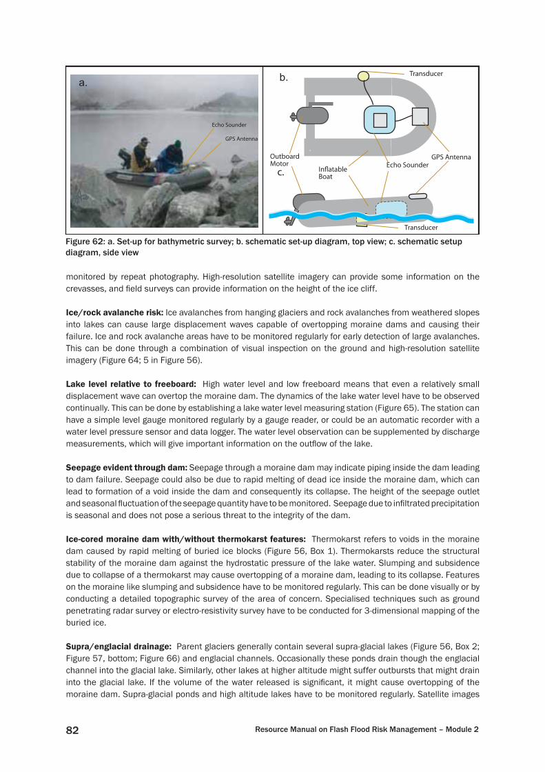
Resource Manual on Flash Flood Risk Management – Module 282
monitored by repeat photography. High-resolution satellite imagery can provide some information on the crevasses, and fi eld surveys can provide information on the height of the ice cliff.
Ice/rock avalanche risk: Ice avalanches from hanging glaciers and rock avalanches from weathered slopes into lakes can cause large displacement waves capable of overtopping moraine dams and causing their failure. Ice and rock avalanche areas have to be monitored regularly for early detection of large avalanches. This can be done through a combination of visual inspection on the ground and high-resolution satellite imagery (Figure 64; 5 in Figure 56).
Lake level relative to freeboard: High water level and low freeboard means that even a relatively small displacement wave can overtop the moraine dam. The dynamics of the lake water level have to be observed continually. This can be done by establishing a lake water level measuring station (Figure 65). The station can have a simple level gauge monitored regularly by a gauge reader, or could be an automatic recorder with a water level pressure sensor and data logger. The water level observation can be supplemented by discharge measurements, which will give important information on the outfl ow of the lake.
Seepage evident through dam: Seepage through a moraine dam may indicate piping inside the dam leading to dam failure. Seepage could also be due to rapid melting of dead ice inside the moraine dam, which can lead to formation of a void inside the dam and consequently its collapse. The height of the seepage outlet and seasonal fl uctuation of the seepage quantity have to be monitored. Seepage due to infi ltrated precipitation is seasonal and does not pose a serious threat to the integrity of the dam.
Ice-cored moraine dam with/without thermokarst features: Thermokarst refers to voids in the moraine dam caused by rapid melting of buried ice blocks (Figure 56, Box 1). Thermokarsts reduce the structural stability of the moraine dam against the hydrostatic pressure of the lake water. Slumping and subsidence due to collapse of a thermokarst may cause overtopping of a moraine dam, leading to its collapse. Features on the moraine like slumping and subsidence have to be monitored regularly. This can be done visually or by conducting a detailed topographic survey of the area of concern. Specialised techniques such as ground penetrating radar survey or electro-resistivity survey have to be conducted for 3-dimensional mapping of the buried ice.
Supra/englacial drainage: Parent glaciers generally contain several supra-glacial lakes (Figure 56, Box 2; Figure 57, bottom; Figure 66) and englacial channels. Occasionally these ponds drain though the englacial channel into the glacial lake. Similarly, other lakes at higher altitude might suffer outbursts that might drain into the glacial lake. If the volume of the water released is signifi cant, it might cause overtopping of the moraine dam. Supra-glacial ponds and high altitude lakes have to be monitored regularly. Satellite images
Transducer
Transducer
Echo SounderGPS AntennaOutboard
MotorInflatableBoat
GPS Antenna
Echo Sounder
a.b.
c.
Figure 62: a. Set-up for bathymetric survey; b. schematic set-up diagram, top view; c. schematic setup diagram, side view

83Chapter 6: Hazard-specifi c Flash Flood Management Measures
Glacial lake
Crevasses
Glacial lake
Ice cliff
Crevasses
Figure 63: Terminus of the Trakarding glacier, the parent glacier of Tsho Rolpa glacial lake, Nepal, showing a series of crevasses in plan view and frontal view
Sou
rce:
Goo
gle
Eart
h (t
op);
Aru
n B
. Shr
esth
a (b
otto
m)
can provide multi-temporal information on the development of supra-glacial ponds and high altitude lakes in the surrounding areas.
Estimation of peak outfl ow discharge: Sophisticated computer models are available to estimate the peak discharge of a GLOF. Due to limited resources and expertise, it is not always possible to do a detailed modelling exercise. A simple method can also provide a reasonably good estimate of the outburst magnitude.
Costa and Schuster (1988) suggested the following equation for predicting peak outfl ow discharge from a GLOF: Q = 0.00013(Pe)
0.60
Where Q is peak discharge in m3/s, and Pe is potential energy in joules.
Pe is the energy of the lake water behind the dam prior to failure and can be calculated using the equation:
Pe = Hd x V x γ
Popov (1991) suggested the following equation for predicting fl ash fl ood peak discharge due to glacier outburst:
Q = 0.0048V 0.896

Resource Manual on Flash Flood Risk Management – Module 284
Hanging glaciers
Lake
Hanging glaciers
Lake
Figure 64: Hanging glaciers near a glacial lake: frontal view (top) and plan view (bottom)
Sou
rce:
Goo
gle
Eart
h (b
otto
m);
Aru
n B
. Shr
esth
a (t
op)

85Chapter 6: Hazard-specifi c Flash Flood Management Measures
The peak discharge depends on the volume of the glacial lake (V). The lake volume is generally not available unless a detailed bathymetric survey has been conducted. The surface area of the lake, however, can be easily derived from maps of satellite imageries. The volume can then be calculated using the following formula suggested by Huggel et al. (2002):
V = 0.104A 1.42
Peak outburst depends on the nature of the outburst, i.e., the duration of the outburst, the nature of the outburst hydrograph, and the size and geometry of the dam breach. In the simple approach, a triangular breach hydrograph is assumed and the duration of the outburst is assumed as 1000s. Huggel et al. (2002) suggest that most outbursts last between 1000 and 2000 seconds, and the peak discharge is calculated by:
tVQ 2=
Figure 65: An automatic weather station equipped with a lake water-level recorder, Lirung, Nepal
Figure 66: Parent glaciers of Imja Lake, Nepal, showing supra-glacial ponds
Glacial lake Supra-glacialponds
Sou
rce:
Goo
gle
Eart
h

Resource Manual on Flash Flood Risk Management – Module 286
Estimation of area that can be impacted by a GLOFThe hazard assessment should include a rough estimate of the area potentially affected by a lake outburst. A worst-case scenario is generally followed for delineating the area that could be affected. The runout (travel) distance of an outburst is related to the amount of debris available to be mobilised. Outburst fl oods with a higher content of solid material form debris fl ows and stop abruptly, whereas GLOFs with predominantly water attenuate more gradually.
To roughly estimate the maximum affected area, the peak discharge is used to estimate the overall slope of the outburst fl ood (the average slope between the starting and the end points of an outburst event). Figure 67 shows the relationship between maximum outfl ow discharge and critical runout slope. For instance, an outfl ow discharge of 100 m3/s gives a critical slope of 2.75.
Figure 68 shows the profi le of a river channel. The critical slope of 2.75 means the fl ood will have an effect up to a distance of 20 km (point 3 in Figure 68).
GLOF risk mappingGLOF risk mapping is an important tool to understand the areas likely to be impacted by a GLOF and to understand the vulnerability of those areas, and will help in planning mitigation measures. Detailed descriptions of GLOF risk mapping can be found in Shrestha et al. (2006) and Bajracharya et al. (2007 a and b). The process involves estimating the discharge hydrograph at the outlet (breach). This can be done using dam break models or by simple calculation assuming the breach size and the lake drawdown rate. The hydrograph is routed through the river reach to fi nd the peak discharge and fl ood height at the locations of interest. An inundation map is prepared by overlaying the fl ood height over the terrain map. Overlaying a socioeconomic vulnerability map based on the information mentioned in Chapter 4 will give the risk map of the area. See Chapter 4 for details on risk assessment.
Terrain AnalysisGLOF is a complex phenomenon involving fl oods, sediment transport, debris fl ows, landslides, and others, which cannot be accurately predicted or foreseen. Terrain analysis can be a good indicator of the magnitude of what might happen during a GLOF event. Terrain analysis is a good tool to verify the results of a hazard map. Bajracharya et al. (2007b) provides a detailed description of terrain analysis.
2.75 o 100 m 3/s
2
1
3
Elev
atio
n (m
asl)
0
1000
2000
3000
4000
5000
6000
0 5000 10000 15000 20000
Lake
Distance from the lake (metres)
5.5 o 25 m 3/s
18 o 2 m 3
/s
Figure 68: Longitudinal profi le of a stream and runout distances for different peak outfow discharges
?
Cri
tica
l slo
pe
(oC
)
Max discharge (m3/s)
Debris flow
Flood wave
2,75
100
Figure 67: Relation between peak discharge and overall slope of runout distance of lake outburst based on data from the Alps
Sou
rce:
Bas
ed o
n H
ugge
l et
al. 2
00
2; H
ugge
l et
al. 2
00
4

87References
ReferencesAgeta, Y.; Kadota, T. (1992) ‘Predictions of Changes of Glacier Mass Balance in the Nepal Himalaya and
Tibetan Plateau: A Case Study of Air Temperature Increase for Three Glaciers.’ In Annals of Glaciology, 16: 89-94
Alexander, D. (1993) Natural Disasters. New York: Chapman and Hall
APFM (2004) Integrated Flood Risk Management. Geneva: Associated Program on Flood Management
Archer, D. (2001) Recent Glacial Outbursts, Debris Flows and Dam Breaks in Chizer/Gilgit Basins of Northern Pakistan. Lahore: WAPDA/GTZ/VSO
Bajracharya, B.; Shrestha, A. B.; Rajbhandari, L. (2007a) ‘Glacial Lake Outburst Floods in the Sagarmatha Region: Hazard Assessment Using GIS and Hydrodynamic Modelling’. In Mountain Research and Development, 27: 336-344
Bajracharya, S.R.; Mool, P.K.; Shrestha, B.R. (2007b) Impact of Climate Change on Himalayan Glaciers and Glacial Lakes: Case Studies of GLOF and Associated Hazards in Nepal and Bhutan. Kathmandu: ICIMOD
Blakie, P.; Cannon, T.; Davis, I.; Wisner, B. (1994) At Risk -- Natural Hazards, People’s Vulnerability and Disasters. London: Routledge
Brilly, M. (2001) ‘The Integrated Approach to Flash Flood Management’. In E. Gruntfest and J. Handmer (eds) Coping with Flash Floods, pp 103-114. Dordrecht: Kluwer Academic Publishers
Chalise, S.R.; Khanal, N.R. (2001) ‘An Introduction to Climate, Hydrology and Landslide Hazards in the Hindu Kush-Himalayan Region: Landslide Hazard Mitigation in the Hindu Kush-Himalaya’. In Tianchi, L.; Chalise, S.R.; Upreti, B.N. (eds) Landslide Hazard Mitigation in the Hindu Kush-Himalaya, pp 51-62. Kathmandu: ICIMOD
Chow, V.T. (1984) Handbook of Applied Hydrology: A Compendium of Water Resources Technology. New York: McGraw-Hill
Chow, V.T.; Maidment, D.R.; Mays, L.W. (1988) Applied Hydrology. Singapore: McGraw-Hill
Colombo, A.G.; Hevas, J.; Arllam, A.L.V. (2002) Guidelines on Flash Floods Prevention and Mitigations. Ipsra (Italy): NEIDES
Costa, J.E. (1983) ‘Paleohydraulic Reconstruction of Flash-fl ood Peaks from Boulder Deposits in the Colorado Front Range’. In Geological Society of America Bulletin, 94: 986-1004
Costa, J.E.; Schuster, R.L. (1988) ‘The Formation and Failure of Natural Dams’. In Geological Society of America Bulletin, 100: 1054-1068
Cutter, S.L. (1996) ‘Vulnerability to Natural Hazards.’ In Progress in Human Geography, 20: 529-539
Dams, Rivers and People (2004) Pareechu Lake Developments. New Delhi: Dams, Rivers & People
Deoja, B.; Dhital, M.; Thapa, B.; Wagner, A. (1991) Mountain Risk Engineering Handbook, Subject Background: Part I. Kathmandu: ICIMOD
Dhital, M.R.; Khanal, N.; Thaa, K.B. (1993) The Role of Extreme Weather Events, Mass Movements, and Land Use Changes in Increasing Natural Hazards. Kathmandu: ICIMOD
DHM/DPTC (1994) 1993 Flood Assessment of Bagmati River and East Rapti River. Kathmandu: Department of Hydrology and Meteorology and Disaster Prevention Technical Centre

Resource Manual on Flash Flood Risk Management – Module 288
DMTP (1997) Introduction to Hazards. Geneva: United Nations Disaster Management Training Programme (UN-DMTP)
Domroes, M. (1979) ’Temporal and Spatial Variations of Rainfall’. In Journal of Nepal Research Centre, 2: 49-67
Dunning, S.A.; Rosser, N.J.; Petley, D.N.; Massey, C.R. (2006) ‘Formation and Failure of the Tsatichhu Landslide Dam, Bhutan’. In Landslides, 3: 107-113
DWIDP (2005) Disaster Review 2004, Series XII. Kathmandu: Department of Water Induced Disaster Prevention, Nepal
Fujita, K.; Nakazawa, F.; Rana, B. (2001) ‘Glaciological Observation on Rika Samba Glacier in Hidden Valley, Nepal Himalayas, 1998 and 1999’. In Bulletin of Glaciological Research, 18: 31-35
Georgakakos, K. (2004) Mitigating Adverse Hydrological Impacts of Storms on a Global Scale with High Resolution Global Flash Flood Guidance System. International Conference on Storms. Storms Science to Disaster Mitigation, Brisbane, 5-9 July 2004
Gouldby, B.; Samuals, P. (2005) Language of Risk. Wallingford: FloodSite
Heyman, B.N.; Davis, C.; Krumpe, P.F. (1991) ‘An Assessment of Worldwide Disaster Vulnerability’. In Disaster Management, 4: 1-23
Huggel, C.; Haeberli, W.; Kääb, A.; Bieri, D.; Richardson, S. (2004) ‘An Assessment Procedure for Glacial Hazards in the Swiss Alps’. In Canadian Geotechnical Journal, 41: 1068-1083
Huggel, C.; Kääb, A.; Haeberli, W.; Teysseire, P.; Paul, F. (2002) ‘Remote Sensing Based Assessment of Hazards from Glacial Lake Outbursts: A Case Study in the Swiss Alps’. In Canadian Geotechnical Journal, 39: 316-330
ICIMOD (2007) Inventory of Glaciers, Glacial Lakes, and Identifi cation of Potential Glacial Lake Outburst Flood (GLOFs) Affected by Global Warming in the Mountains of Himalayan Region. Kathmandu: ICIMOD
IDNDR (1997) Guiding Principles for Effective Early Warning. Geneva: United Nations International Decade for Natural Disaster Reduction (IDNDR)
ISDR (2004) Living with Risk. A Global Review of Disaster Reduction Initiatives. Hyogo (Japan): United Nations International Strategy for Disaster Reduction (UN/ISDR)
ISDR (2005) ‘Hyogo Framework for Action 2005-20015’. Presented at World Conference on Disaster Reduction, Kobe. Hyogo (Japan): United Nations International Strategy for Disaster Reduction (UN/ISDR)
Iturrizaga, L. (1997) ‘The Valley of Shimshal - A Geogrphic Potrait of a Remote High Mountain Settlement and its Pastures with Reference to Environmental Habitat Condtitions in the North-West Karakorum (Pakistan)’. In GeoJournal, 42: 303-328
Iturrizaga, L. (2005a) ‘New Observations on Present and Prehistorical Glacier-Dammed Lakes in Shimshal Valley (Karakorum Mountains)’. In Journal of Asian Earth Sciences, 24: 545-555
Iturrizaga, L. (2005b) ‘The Historical Saklei Shuyinj and Chateboi Glacier Dams as Triggers for Lake Outburst Cascades in the Karambar Valley, Hindukush’. In The Island Arc, 14: 389-399
Ives, J.D. (1986) Glacial Lake Outburst Floods and Risk Engineering in the Himalaya. Kathmandu: ICIMOD
Jarrett, R.D.; Costa, J.E.; (2006) ‘1976 Big Thompson Flood-Thirty Years Later’. In U.S. Fact Sheet-2006-3095. Washington: U.S. Geological Survey (USGS)
Jonkman, S.N. (2005) ‘Global Perspectives on Loss of Human Life Caused by Floods’. In Natural Hazards, 34: 151-175

89References
Kadota, T.; Fujita, K.; Seko, K.; Kayastha, R.B.; Ageta, Y. (1997) ‘Monitoring and Prediction of Shrinkage of a Small Glacier in Nepal Himalaya’. In Annals of Glaciology, 24: 90-94
Kelsch, M.; Caporali, E.; lanza, L.G. (2001) ‘Hydrometeorology of Flash Floods’. In Gruntfest, E.; Handmer , J. (eds) Coping with Flash Floods, pp 19-35. Dordrecht/Boston/London: Kluwer Academic Publishers
Kulkarni, A.V.; Rathore, B.P.; Mahajan, S.; Mathur, P. (2005) ‘Alarming Retreat of Parbati Glacier, Beas Basin, Himachal Pradesh’. In Current Science, 88: 1844-1850
Kron, W. (2005) ’Floodrisk=Hazard*Values*Vulnerability’. In Water International, 30: 58-68
Li, Tianchi (1994) Landslide Hazard Assessment in Mountain Areas of China, Remote Sensing Application to the Planning and Management of Environment, Natural Resources and Physical Infrastructure. Kathmandu: UN/CDG/ESA/ICIMOD
Mavis, I.D.; Laushey, L.M. (1949) ‘Formula for Velocity of Beginning of Bedload Movement is Reappraised’. In Civil Engineering, 19: 38-39
Mei’e, R.; Renzhang, Y.; Haoshend, B. (1985) An Outline of China’s Physical Geography. Beijing: Foreign Language Press
Messner, F.; Meyer, V. (2005) Flood Damage, Vulnerability and Risk Perceptions – Challenge for Flood Damage Research. Leipzig: UFZ-Umweltforschungszentrum Leipzy-Halle
Mizuyama, T.; Satohuka, Y.; Ogawa, K.; Mori, T. (2006) Estimating the Outfl ow Discharge Rate from Landslide Dam Outbursts, Disaster Mitigation of Debris Flows, Slope Failures and Landslides. Tokyo: Universal Academy Press
Mool, P.; Bajracharya, S.R.; Joshi, S.P. (2001) Inventory of Glaciers, Glacier Lakes and Glacial Lake Outburst Floods, Monitoring and Early Warning System in the Hindu Kush-Himalayan Region. Kathmandu: ICIMOD/UNEP
Mool, P.; Che, T.; Bajracharya, S.R.; Shrestha, B.R. (2005) ‘Monitoring of Glaciers and Glacial Lakes from 1970s to 2000 in Poiqu Basin, Tibet Autonomous Region, PR China’. Paper presented at the International Workshop on Flash Floods Management and Sustainable Development, Lhasa, 23-28 October 2005
New, M.; Lister, D.; Hulme, M.; Makin, I. (2002) ‘A High-resolution Data Set of Surface Climate Over Global Land Areas’. In Climate Research, 21: 1-25
Popov, N. (1991) ‘Assessment of Glacial Debris Flow Hazard in the North Tien-Shan’. Proceedings of the Soviet-China-Japan Symposium and Field Workshop on Natural Disasters, 384–391. 2-17 September 1991, Tian-Shan
Reynolds, J. M. (1999) ‘Glacial Hazard Assessment at Tsho Rolpa, Rolwaling, Central Nepal’. Quarterly Journal of Engineering Geology, 32: 209-214
RGSL (2003) Methods of Glacier and Lake Inventory Compilation with Specifi c Reference to Hazard Assessment. Flintshire: Flintshire Reynolds Geo-sciences Limited (RGSL)
Richardson, S.D.; Reynolds, J.M. (2000) ‘An Overview of Glacial Hazards in the Himalayas’. In Quarternary International, 65/66(1): 31-47
Schuster, R.L.; Alford, D. (2004) ‘Usoi Landslide Dam and Lake Sarez, Pamir Mountains, Tajikstan’. In Environmental and Engineering Geoscience, 10: 151-168
Shamshad, K.M. (1988) The Meteorology of Pakistan. Karachi: Royal Book Company
Shang, Y.; Yang, Z.; Li, L.; Liu, D.; Liao, Q;. Wang, Y. (2003) ‘A Super-large Landslide in Tibet in 2000: Background, Occurrence, Disaster, and Origin’. Geomorphology, 54: 225-243
Sherard, J.L. (1979) ‘Sinkholes in Dams of Coarse, Broadly Grained Soils’. In International Conference on Large Dams, pp 25-35. New Delhi: Transactions

Resource Manual on Flash Flood Risk Management – Module 290
Shing, P.; Bengtsson, L. (2004) ‘Hydrology Sensitivity of a Large Himalayan Basin to Climate Change’. In Hydrological Processes, 18: 2363-2385
Shing, P.; Bengtsson, L. (2005) ‘Impact of Warmer Climate on Melt and Evaporation for the Rainfed, Snowfed and Glacierfed Basins in the Himalayan Region’. In Journal of Hydrology, 300: 140-154
Shiyin, L.; Zichu, X.; Guoping, S.; Li, M.; Ageta, Y. (1996) ‘Mass Balance of Kangwure (Flat-top) Glacier on the North Side of Mt. Xixiabangma, China’. In Bulletin of Glacier Research, 14: 37-43
Shrestha, A. (2005) Vulnerability Assessment of Weather Disasters in Syangja District, Nepal: A Case Study of Putalibazar Municipality. Washington D.C.: Advanced Institute on Vulnerability to Global Environmental Change/ Global Change System for Analysis Research and Training (START)
Shrestha, A.B.; Bajracharya, B.; Rajbhandari, L. (2006) ‘Glacier Lake Outburst Flood Hazard Mapping of Sagarmatha National Park’. In Sharma, K.P.; Jha, R. (eds) Workshop on Flood Forecasting Management in Mountainous Areas. Kathmandu: Department of Hydrology and Meteorology
Shrestha, A.B.; Budhathoki, K.P.; Shrestha, R.K.; Adhikari, R. (2004) ‘Bathymetric Survey of Tsho Rolpa Glacier Lake 2002’. In Journal of Hydrology and Meteorology, 1: 13-15
Shrestha, A.B.; Shrestha, M.L. (2006) Glacier Lake Outburst Flood and Other Flash Floods in Nepal. In Xu, Jianchu; Eriksson, M.; Ferdinand, J.; Merz, J. (eds) Managing Flash Floods and Sustainable Development in the Himalayas: International Workshop on Flash Floods. Kathmandu: ICIMOD
Strand, R.I. (1977) Sedimentation in Design of Small Dams. Washington: U.S. Bureau of Reclamation
Swaminathan, M.S. (1980) ‘Plant Breeding in India: Some Experiments and Ecological Experiences in the North Eastern Hill Region’. In Singh, T.; Kau, J. (eds) Studies in Himalayan Ecology and Development Strategies, pp 152-172. New Delhi: The English Book Store
Swanson, F.J.; Oyagi, N.; Tominaga, M. (1986) ‘Landslide Dams in Japan’. In Schuster, R.L. (ed) Landslide Dams – Processes, Risks, Mitigations, American Society of Civil Engineers Geotechnical Special Publication 3: 131-145. Reston: American Society of Civil Engineers
UNDP/BCPR (2004) Reducing Disaster Risk: A Challenge for Development. New York: United Nations Development Program, Bureau for Crisis Prevention and Recovery (UNDP/BCPR)
UNU-EHS (2006) Components of Risk: A Comparative Glossary. Bonn: United Nations University, Institute for Environment and Human Security (UNU-EHS)
Watts, M.J.; Bohle, H.G. (1993) ‘The Space of Vulnerability: The Casual Structure of Hunger and Famine’. In Progress in Human Geography, 17: 43-67
WECS/DHM (1990) Methodologies for Estimating Hydrologic Characteristics of Ungauged Locations in Nepal (Vol. 1, Main Report). Kathmandu: Water and Energy Commission Secretariat and Department of Hydrology and Meteorology (WECS/DHM)
WECS (1987) Erosion and Sedimentation in Nepal. Kathmandu: Water and Energy Commission Secreteriat (WECS)
Weichselgartner, J. (2001) Naturgefahren als soziale Konstruktion. Dissertation presented to the Faculty of Mathematics and Natural Sciences, University of Bonn, Germany
Williams, G.P. (1983) ‘Paleohydrological Methods and Some Examples from Swedish Fluvial Environments. I. Cobble and Boulder Deposits’. In Geografi ska Annaler, 65A: 227-243
WWF (2005) An Overview of Glaciers, Glacier Retreat and its Subsequent Impacts in Nepal, India and China. Kathmandu: WWF Nepal Program
Xu, D. (1985) ‘Characteristics of Debris Flows Caused by Outburst of Glacier Lakes in Boqu River in Xizang, China, 1981’. In GeoJournal, 17: 569-580

91References
Xu, Jianchu; Eriksson, M; Ferdinand, J.; Merz, J. (2006) Managing Flash Floods and Sustainable Development in the Himalayas: International Workshop on Flash Floods. Kathmandu: ICIMOD
Xu, Jianchu; Shrestha, A.; Vaidya, R.; Eriksson, M.; Hewitt, K. (2007) The Melting Himalayas: Regional Challenges and Local Impacts of Climate Change on Mountain Ecosystems and Livelihoods. Kathmandu: ICIMOD
Yamada, T. (1998) ‘Monitoring of Glacier Lake and Its Outburst Floods in Nepal Himalaya’. In Japanese Society of Snow and Ice: Monograph No. 1: 96
Zhu, P.; Li, Tianchi (2000) Flash Flooding Caused by Landslide Dam Failure. In ICIMOD Newsletter 38, pp 4-5
Zhu, P. Y.; Wang, C. H.; Wang, Y. C. (2003) ‘Formation of an Exceptionally Serious Outburst Flood from a Landslide Dam in Tibet’. In Newsletter of Japanese Landslide Society, 14/15: 23-25
Zurick, D.; Pacheco, J.; Shrestha, B.; Bajracharya, B. (2006) Atlas of the Himalaya. Kathmandu: ICIMOD

ISBN 978 92 9115 095 3International Centre for Integrated Mountain DevelopmentKhumaltar, Lalitpur, GPO Box 3226, Kathmandu, NepalTel: +977 1 5003222, Fax: +977 1 5003277 / 5003299Email: [email protected] www.icimod.org

CD-ROM with PDF fi les of
Resource Manual on Flash Flood Risk Management Module 2: Non-structural Measures
andAnnexes
List of AnnexesAnnex 1 : Hazard, Vulnerability, and Risk Analysis Annex 2 : Application of GIS to Flood Hazard MappingAnnex 3 : Guiding Principles for Effective Early WarningAnnex 4 : Runoff Curve NumbersAnnex 5 : Training Manual on Flash Flood Modelling using HEC-GEOHMS and HEC HMSAnnex 6 : Inventory of Glaciers and Glacial Lakes, and Identifi cation of Potentially Dangerous Glacial
Lakes
If the CD-ROM is missing, the Annexes can be downloaded from www.books.icimod.org. Additional CDs can be obtained from ICIMOD.