Resource Management of Highly Configurable Tasks

April 26, 2004

Jeffery P. Hansen Sourav Ghosh

Raj Rajkumar John P. Lehoczky

Carnegie Mellon University

Outline

• Radar Tracking Problem

• Introduction to Q-RAM

• Application of Q-RAM to Radar Tracking

• Slope-Based Traversal

• Fast Traversal

• Experimental Results

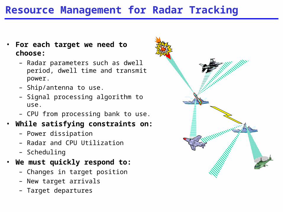
• For each target we need to choose:– Radar parameters such as dwell

period, dwell time and transmit power.

– Ship/antenna to use.

– Signal processing algorithm to use.

– CPU from processing bank to use.

• While satisfying constraints on:– Power dissipation

– Radar and CPU Utilization

– Scheduling

• We must quickly respond to:– Changes in target position

– New target arrivals

– Target departures

Resource Management for Radar Tracking

0%

50%

100%

0%

50%

100%

Radar Resource Management Approaches

• Existing solutions use operational doctrine to make resource allocation decisions.

– Resources allocated to tasks in order of importance based only on each task’s characteristics.

– Some problems with this approach are:• Important tasks can starve tasks of slightly

lower priority.• Does not make best use of resources.• Difficulty in predicting viable scenarios.

• QoS-based optimization considers resource tradeoffs and relative task importance.

– Resources allocated in proportion to importance.– Tasks can have unlimited access to resource

when demand is low.– Tasks can not starve other tasks of similar

importance.– Operator can dynamically change importance.

Priority-Based Allocation

QoS-Based Optimization

QoS Optimization with Q-RAM

Image Resolution

Fra

mes

/sec

.

• QoS modeled as an n-dimensional space – Each set-point in the space has an associated

“utility” value representing user satisfaction.– Utility values can be assigned individually or

via dimension-wise utility functions. • A single QoS set-point can be realized by multiple

“Resource Options”.– Resource trade-offs– QoS Routing

• Optimization goal is to maximize total system utility while meeting resource constraints.

• Per-user weights give higher priority to “important” users.

• Near optimal solution for search space of over a trillion QoS setpoint combinations found in under 1 sec.

QoS Model of Radar Tracking Problem

Resources• Radar bandwidth• Short-term power• Long-term power• CPUs• Memory

Operational Dimensions• Dwell Period• Dwell Time• Transmit Power• Tracking Algorithm• # of task replicas

Environment• Distance • Speed• Direction• Maneuvering• Counter Measures

ThreatAssessment

QoS Dimensions• Track Error• Target Drop Probability• Reliability

MarginalUtility

Control

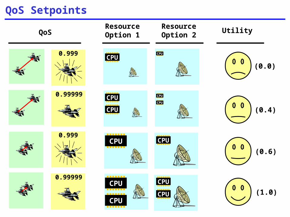
QoS Setpoints

QoSResourceOption 1

ResourceOption 2

Utility

(0.0)

(0.4)

(0.6)

(1.0)

CPU0.999

0.999

CPU

CPU

CPU

CPU

CPU

0.99999

0.99999

CPU CPU

CPU

CPU

CPU

CPU

Radar Constraint/Resource Model

Per Antenna Constraints:

Global Constraints:maxP maxC

1H

1U 2U

2H …

R1 R2Global

Computing (Cmax) –

Limit on processing capabilities for tracking targets.

Power (Pmax) – Limit on

power that can be provided to power radars.

Heat (Hi ) – Limit on heat

that can be dissipated per unit time.

Utilization(Ui ) – Limit on

fraction of time radar can be in continuous use.

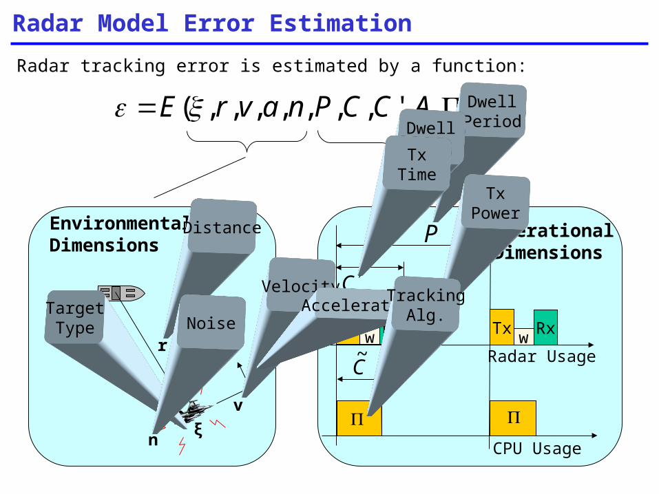
Radar Model Error Estimation

Radar tracking error is estimated by a function:

),,',,,,,,,( ACCPnavrE

EnvironmentalDimensions

r

v

a

ξn

C~

PC

C

A

CPU Usage

Radar Usage

OperationalDimensions

wTx Rx

wTx Rx

TargetType

Distance

VelocityAcceleration

Noise

DwellPeriodDwell

TimeTxTime

TxPower

TrackingAlg.

Setpoint Explosion Problem

• Concave majorant algorithm used by Q-RAM requires O(n ln n) and must examine every setpoint.

• For applications with more than a few operational dimensions, the number of setpoints can be very large – With k dimensions having m settings, there

are mk setpoints.– Even a linear algorithm may take a long time.

One Dimension

Two Dimensions

Three Dimensions Four Dimensions

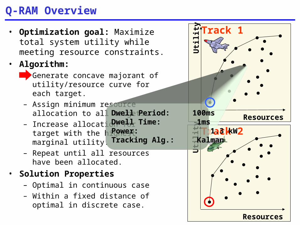
• Optimization goal: Maximize total system utility while meeting resource constraints.

• Algorithm:– Generate concave majorant of

utility/resource curve for each target.

– Assign minimum resource allocation to all targets.

– Increase allocation for target with the highest marginal utility.

– Repeat until all resources have been allocated.

• Solution Properties– Optimal in continuous case

– Within a fixed distance of optimal in discrete case.

Q-RAM Overview

Resources

Uti

lity

Resources

Uti

lity

Track 1

Track 2

Dwell Period: 100msDwell Time: 1msPower: 1.3 kWTracking Alg.: Kalman

Slope Based Traversal

• Algorithm– Determine minimum and maximum

QoS points.– Eliminate points under the line

connecting them.– Apply concave majorant to remaining

points.

• Initial scan is linear– Reduces number of points to which

we must apply the concave majorant algorithm.

– Some reduction in execution time.– But, still must examine every setpoint.

Compound Resource

Uti

lity

Fast Convex Hull Algorithms

• Resource/utility values associated with setpoints are not random.

• Utilize structure in the resource management problem to reduce this complexity.

• For most operational dimensions, an increase in quality on any dimension results in:– Non-decreasing resource consumption.– Non-decreasing utility.

• We call dimensions with the above property “monotonic” dimensions.

• All other dimensions are called “non-monotonic” dimensions. Dwell Period

Tra

nsm

it P

ow

er

R U R U

R U

<1,*>

<2,*><3,*>

<*,1>

<*,2>

<*,3>

<*,4><*,5>

Fast Traversal Methods

Observations of the points on the concave majorant have revealed that for monotonic dimensions:– Concave majorant is usually

composed of sub-sequences of points differing in only one quality index.

– Dimension that is changing may shift as the concave majorant is traversed.

– May need to treat “non-monotonic” dimensions separately.

Compound Resource

Uti

lity

<1,1>

<1,2>

<1,3>

<1,4> <2,4> <3,4> <3,5>

Fast Traversal Algorithms

• FOFT: First Order Fast Traversal Algorithm:– Make the minimum QoS point the

current point.

– Examine points adjacent in the quality index space to the current point.

– Choose next point with highest marginal utility.

– Repeat until reaching maximum QoS point.

– Apply concave majorant to resulting set of points.

• Generates nearly the same set of points as full concave majorant.

• Explicitly examines only a small subset of the possible setpoints.

• Utility values within a few percent of standard Q-RAM algorithm.

Dwell Period

Tra

nsm

it P

ow

er

Compound Resource

Uti

lity

R*

U

R*

U

R*

UR*

U

R*

U

R*

U

R*

UR*

U

R*

UR*

U

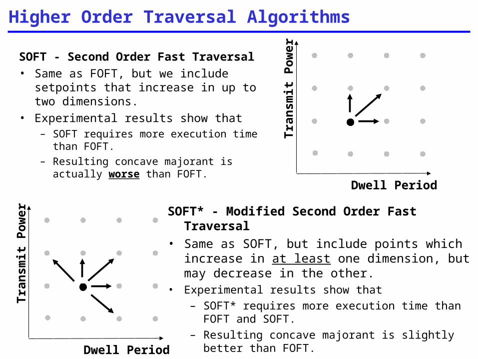
Higher Order Traversal Algorithms

SOFT* - Modified Second Order Fast Traversal• Same as SOFT, but include points which

increase in at least one dimension, but may decrease in the other.

• Experimental results show that

– SOFT* requires more execution time than FOFT and SOFT.

– Resulting concave majorant is slightly better than FOFT.

Dwell Period

Tra

nsm

it P

ow

er

SOFT - Second Order Fast Traversal• Same as FOFT, but we include setpoints

that increase in up to two dimensions.• Experimental results show that

– SOFT requires more execution time than FOFT.

– Resulting concave majorant is actually worse than FOFT.

Dwell Period

Tra

nsm

it P

ow

er

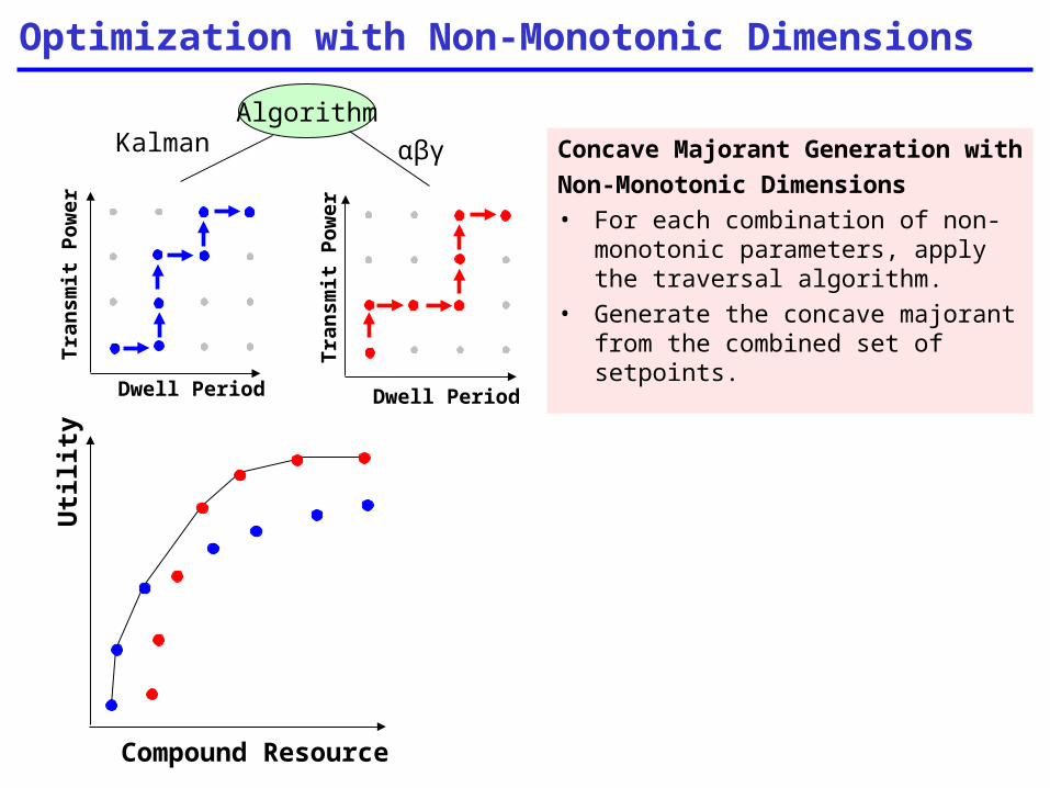
Optimization with Non-Monotonic Dimensions

Compound Resource

Uti

lity

Dwell Period

Tra

nsm

it P

ow

er

Dwell Period

Tra

nsm

it P

ow

er

AlgorithmKalman αβγ Concave Majorant Generation with

Non-Monotonic Dimensions

• For each combination of non-monotonic parameters, apply the traversal algorithm.

• Generate the concave majorant from the combined set of setpoints.

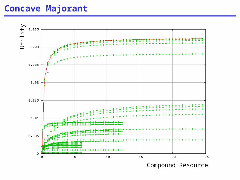
Concave Majorant

Compound Resource

Util

ity

Slope-Based Concave Majorant

FOFT Concave Majorant Approximation

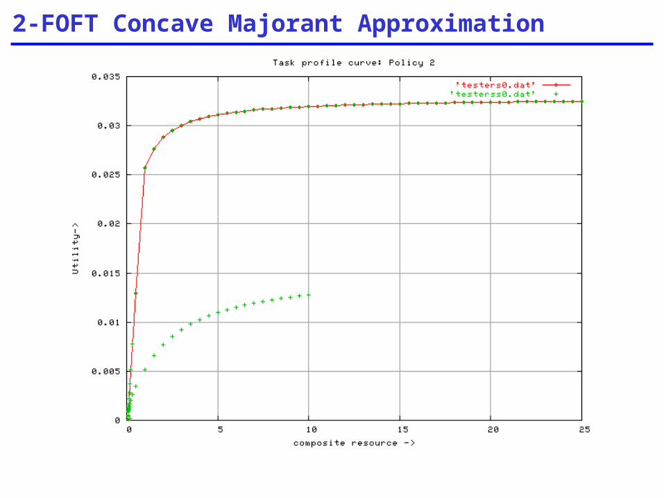
2-FOFT Concave Majorant Approximation

Global Utility

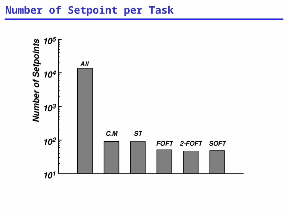
Number of Setpoint per Task

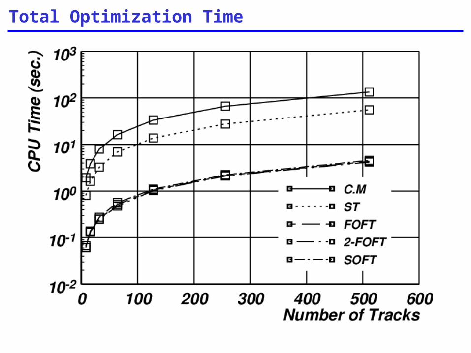
Total Optimization Time

Conclusion

• Approach Overview– Leverage structure in the setpoint space to generate concave majorant

approximation.

– Concave majorant estimated by following the adjacent point on the monotonic dimension with the highest marginal utility.

– Algorithm repeated for all combinations of non-monotonic dimensions.

• Benefits of Approach– Significantly reduces the number of setpoints that must be examined to

obtain a concave majorant estimate.

– Complexity is sub-linear in the number of setpoints.

– Works best when most operational dimensions are monotonic.

• Results– No significant reduction in solution quality.

– Order of magnitude reduction in optimization time.