Embed Size (px)
Citation preview
Resource Distribution and Productivity Analysis
within Pakistan’s Agriculture
A Case Study
Dissertation
zur Erlangung des akademischen Grades
doctor rerum agriculturarum
(Dr. rer. agr.)
eingereicht an der
Landwirtschaftlich-Gärtnerischen Fakultät
der Humboldt-Universität zu Berlin
von
M.Sc (hons) Agri. Economics, Hafiz Zahid Mahmood
geb. 17.02.1972, Ali Pur Chatta, Gujranwala, Pakistan
Präsident der Humboldt-Universität zu Berlin
Prof. Dr. Christoph Markschies
Dekan der Landwirtschaftlich Gärtnerischen Fakultät
Prof. Dr. Dr. h.c. Otto Kaufmann
Gutachter:
1. Prof. Dr. Hans E. Jahnke
2. Prof. Dr. Dr. h.c. Dieter Kirschke
Tag der mündlichen Prüfung: 24-07-2009

i
DEDICATION
Dedicated to my beloved (late) father, who strongly desired to see me as a Ph.D doctor.
Perhaps, without his prayers and inspiring motivations, it was not possible for me to accom-
plish this task.

ii
ACKNOWLEDGEMENT
In the name of Allah (God) the most merciful, compassionate and beneficent who bestowed me with
intellect and supporting people to accomplish this hard and challenging task of Ph.D. I also indebted
for granting me passionate and accommodating supervisor like Professor Dr Hans E Jahnke.
I am grateful from the core of my heart, the most important individual in supervising this research:
my advisor Professor Dr Hans E Jahnke for his excellent guidance and enthusiastic support for my
research and professional development. It was not possible for me to proceed ahead without his pre-
cious intellectual suggestions and ideas. Furthermore, his remarkable patience, continuous encou-
ragement during tedious work of my data analysis and moral and technical support in write up span
kept me enthusiastic to concentrate more and more on my research work. His critical and keen view
of different drafts of my dissertation helped me to shape my thesis in a final presentable format. I
am, also, thankful to Professor Dr Dieter Kirschke for his kind supervision as a second supervisor
for my Ph.D work. I intend to pay special homage and tribute to (late) Dr Irina Gilbert due to her
polite support and kind help in drafting my research project in the start of my Ph.D.
My bouquets of thanks go to Frau Novak for helping me in data analysis and it was a pleasant expe-
rience to learn a great deal of statistical tools in a motherly affection environment. Special thanks
also goes to Dr Marco Hartmann (my senior) for bestowing me his worthy time for valuable consul-
tations and sharing innovative ideas. I can not forget the help of Frau Meaini who was always ready
to assist me for administrative matters. I am also thankful to all of my colleagues including Hatem
Metwali for providing me vey friendly environment of work.
Moreover, I am highly grateful to Dr Intizar Hussain (International Director of International Net-
work for Participatory Irrigation Management); without his support I could not attain data to pursue
my Ph.D from International Water Management Institute. Furthermore, I also owe to Professor Dr
Muhammad Ashfaq (Chairman Department of Agriculture Economics, University of Agriculture
Pakistan), his kind support make data availability easier for me from the aforesaid organization.
I am grateful for the kind suggestions of different experts during my visit to University of Agricul-
ture Faisalabad, Agriculture Census organization, International Water Management Institute, Punjab
Economic Research Institute etc in search of secondary data. All of my friends deserve special ap-
preciation and bundle of thanks for their encouragement and support to me. My special thanks go to
Shahid Qureshi (PhD Scholar at Technical University, Berlin), Muhammad Qasim (PhD Scholar at
Kassel University, Kassel), Haji Rizwan ul Haq (PhD Scholar at Charite, Berlin), Salman Saeed(
PhD Scholar at Frei University, Berlin) and Hafiz Haroon Idrees (PhD Scholar at Humboldt Univer-

iii
sity Berlin) for their moral and intellectual support. Without disclosing name, I want to pay special
gratitude to my friend who financially bore my last year living expenses. Otherwise, PhD could have
been only a dream for me. Prayers of parents always pave the way to destination and it is not suffi-
cient just to utter thanks to them. My thanks, my heart and soul, and my self, will always be availa-
ble for them because they are solely responsible, from my childhood to current status.
iv
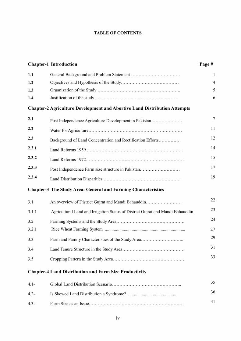
TABLE OF CONTENTS
Chapter-1 Introduction Page #
1.1 General Background and Problem Statement …………………………… 1
1.2 Objectives and Hypothesis of the Study………………………………… 4
1.3 Organization of the Study ……………………………………………….. 5
1.4 Justification of the study ……………………………………………… 6
Chapter-2 Agriculture Development and Abortive Land Distribution Attempts
2.1 Post Independence Agriculture Development in Pakistan………………… 7
2.2 Water for Agriculture……………………………………………………… 11
2.3 Background of Land Concentration and Rectification Efforts…………… 12
2.3.1 Land Reforms 1959 .………………………………………………………. 14
2.3.2 Land Reforms 1972………………………………………………………… 15
2.3.3 Post Independence Farm size structure in Pakistan……………………… 17
2.3.4 Land Distribution Disparities …………………………………………….. 19
Chapter-3 The Study Area: General and Farming Characteristics
3.1 An overview of District Gujrat and Mandi Bahauddin…………………… 22
3.1.1 Agricultural Land and Irrigation Status of District Gujrat and Mandi Bahauddin 23
3.2 Farming Systems and the Study Area………………………………………. 24
3.2.1 Rice Wheat Farming System ........................................................................ 27
3.3 Farm and Family Characteristics of the Study Area……………………….. 29
3.4 Land Tenure Structure in the Study Area…………………………………… 31
3.5 Cropping Pattern in the Study Area…………………………………………. 33
Chapter-4 Land Distribution and Farm Size Productivity
4.1- Global Land Distribution Scenario……………………………………….. 35
4.2- Is Skewed Land Distribution a Syndrome? ............................................ 36
4.3- Farm Size as an Issue………………………………………………………. 41
v
4.4- Evidence of Farm size and Productivity .………………………………… 43
4.4.1- Mis-Specification in Farm Productivity Analysis ………………………… 46
4.4.2- Labour Duality: Mode of Production………………………………….….. 47
4.4.3- Factor Market Imperfections…………………………………………...… 49
4.4.4- Farmers Attributes: Family Size, Age and Education…………………… 51
Chapter-5 Data Sources and Analytical Tools
5.1 Data Sources………………………………………….…………………. 54
5.1.1 Types…………………………………………………………………….. 54
5.1.2 Site Selection and Sampling Methods…………………………………. 55
5.1.3 Data Collection Techniques……………………………………………. 56
5.1.4 Sample Size and Data Cleaning………………………………………… 56
5.2 Analytical Tools ………………………………………………….. 57
5.2.1 Distributional Measures………………………………………………… 57
5.2.2 Total and Partial Factors Productivities………..……………………….. 59
5.2.3 Crop Diversity……………………...……………………………………. 60
5.2.4 Cropping Intensity………………………………………………………. 60
5.2.5 Kruskal Wallis Test: A Test for Research Hypothesis Verification ..…. 61
5.2.6 Econometric Model ……………………………………………….……. 61
Chapter- 6 Land Distributions and Productivity Analysis: A view of Inverse Relationship
6.1 Hypothesis Restated ………………………………………………..…….. 64
6.2 Extent of Land Inequality in the Study Area…………………………. ….. 65
6.2.1 Percentage Distribution of Owned and Operational Farm Area …….. …. 65
6.2.2 Lorenz Curves for Ownership and Operational Holdings…………. …. 67
6.2.3 Gini Coefficient of Ownership and Operational Holdings……………. 70
6.3 Cropping Intensity and Crop Diversity in Study Area.......................... 71
6.3.1 Cropping Intensity……………………………………………………….. 71
6.3.2 Crop Diversity …………………..……………………………………….. 73
6.4 Productivity Analysis in the Study Area ………………………………… 74
6.4.1 Total Factor Productivity (TFP)…………………………………………… 74
vi
6.4.2 Partial Productivity………………………………………………………….. 75
6.4.2.1 Irrigation Productivity………………………………………………………. 76
6.4.2.2 Labour Productivity………………………………………………………… 77
6.4.3 Gross Margins in the Study Area……………………………………….... 78
6.5 Wealth Distribution in the study Area…………………………………….. 79
6.5.1 Income Distribution in the Study Area……………………………………. 80
6.5.2 Farm and Off Farm Income in the Study Area .………………………….. 81
6.5.3 Credit Availability in the Study Areas…………………………………….. 82
6.6 Evidence of Inverse Relationship: Productivity and Factors of Production.. 84
Chapter-7 Discussion
7.1 Inverse Relationship Restated……………………………………………… 88
7.2 Land Distribution…………………………………………………………… 89
7.3 Land distribution, Input Levels and Yield ……………………………….. 92
7.4 Land Distribution and Factor Productivity………………………………… 93
7.5 Land Distribution, Cropping Intensity and Crop Diversity………………. 94
7.6 Small versus Large Farms…………………………………………………. 95
7.7 Inverse Relationship Concluded…………………………………………… 97
Chapter-8 Conclusions and Recommendations 101
Bibliography…………………………………………………………………..…... 107
Appendices……………………………………………………………………………….. 124
viii
LIST OF TABLES
# Titles of Tables
Page
#
2.1 Agriculture Growth Per Capita in Pakistan 1960-2004 (%)……………………………… 8
2.2 Average Yield of Major Crops Per Hectare……………………………………………….. 10
2.3 Water supplies for Irrigation of the Indus Plan……………………………………………. 11
2.4 Land Ownership in Pakistan and Major Agricultural Provinces 1950-55………………. 17
2.5 Land Tenure Structure in Pakistan………………………………………………………… 18
2.6 Number of Farms and Area in Pakistan ………………………………………………….. 19
2.7 Land Gini Ratios in Pakistan 1960-2000........................................................................ 19
3.1 Population of Gujrat and Mandi Bahauddin Districts…………………………………….. 23
3.2 Crop Production Regions in Pakistan……………………………………………………… 26
3.3 Family Characteristics of the Study Area…………………………………………………. 29
3.4 Farm Characteristics of Study Area ……………………………………………………….. 30
3.5 Land Tenure and Tenancy in the Whole Study Area……………………………………. 31
3.6 Land Tenure Structure, Overall Study Area (Percent)…………………………………... 32
3.7 Land Tenure Structure at Small, Medium and Large Farms in Study Area (Percent). 32
4.1 Small Farms as Share of Total Number of Farms and Cultivated Area...................... 42
4.2 Relationship of Farm Size and Cropping Intensity in Increasing Irrigated area......... 44
6.1 Cropping Intensity in the Study Area............................................................................. 72
6.2 Crop Diversity Index....................................................................................................... 73
6.3 Total Factor Productivity in the Study Area (Percent)…………………………………… 75
6.4 Irrigation productivity in the Study Area (Percent)……………………………………….. 76
6.5 Labour productivity in the Study Area (%)………………………………………………… 77
6.6 Gross Margins in the Study Areas (Rupees)……………………………………………… 79
6.7 Income Distribution: Gini Coefficients of various study Location ……………………… 81
6.8 Off and On farm Income Share of the Households in the Study Area (Percent)……… 82
6.9 Regression Results with Dependent Variable Yield Per Hectare (Rupees)…………… 85
ix
LIST OF FIGURES
# Titles of Figures Page #
2.1 Growth in Cultivated Area and Agriculture Labor from 1950-53 to 2000-03………….. 9
2.2 Land and Labor Productivity in Agriculture, in Pakistan………………………………… 9
2.3 Ground water exploitation since 1900 .......................................................................... 12
3.1 Administrative Structure of Pakistan.............................................................................. 21
3.2 Location Map of District Gujrat and M.B.D…………………………………………… 22
3.3 Rice-Wheat farming System in Indus Basin of Pakistan………………………………… 28
3.4 Major Crops Grown in the Study Area …………………………………………………… 34
4.1 Distribution of Agricultural Land Holdings (1990 Round of Agri. Censuses).................. 36
4.2 Equality of Land Distribution and Economic Growth, Selected Countries…………….. 37
4.3 Impact of Skewed Land Distribution on Undernourishment ……………………………... 38
4.4 Unequal Land Ownership and Public Expenditures on Education …………………….. 39
4.5 Farm Size and Output per Unit Area……………………………………………………… 43
4.6 Labour Productivity: The Relationship of Wage Rate, Imputed family labour costs and
Marginal Product………………………………………………………………………….. 48
5.1 Irrigated and Rainfed Areas of District Gujrat and Mandi Bahauddin …………………. 56
5.2 Lorenz Curves for Typical Income Distribution and Perfect Equality 58
6.1 Percentage Distribution of Farm Area of Operational and Ownership Holding in Quin-
tiles……………………………………………………………………………………… 66
6.2 Overall Area: Lorenz Curve for Ownership and Operational Land Holdings…………… 67
6.3 Irrigated Perennial Area: Lorenz Curve for Ownership and Operational Land Holdings 68
6.4 Irrigated Non Perennial Area: Lorenz Curve for Ownership and Operational Land Hold-
ings……………………………………………………………………………………… 68
6.5 Rainfed Area: Lorenz Curve for Ownership and Operational Land Holdings………….. 69
6.6 Gini Coefficient for Ownership and Operational Land Holding in Study area…………. 70
6.7 Cropping Intensity in the Study Area …………………………………………………….. 72
6.8 Lorenz Curves for Income Distribution in the study area………………………………… 80
6.9 Institutional Credit Availability to the Farmers in Study Area (percent)………………… 83
7.1 Advantages of Even and Disadvantages of Skewed Land distribution…………………. 90
7.2 Ranking of Investment and Outcomes as a Consequent Land Distribution……………. 95
8.1 Ranking of Indicators with Reference to Land distribution 103
x
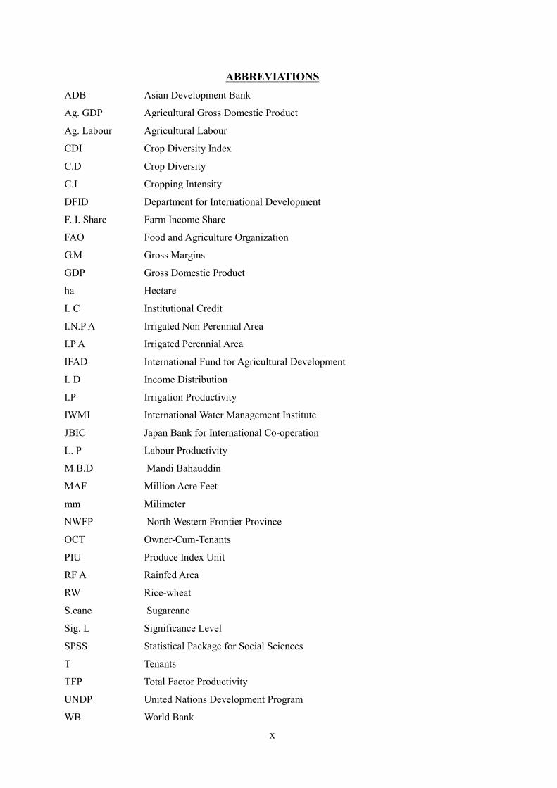
ABBREVIATIONS
ADB Asian Development Bank
Ag. GDP Agricultural Gross Domestic Product
Ag. Labour Agricultural Labour
CDI Crop Diversity Index
C.D Crop Diversity
C.I Cropping Intensity
DFID Department for International Development
F. I. Share Farm Income Share
FAO Food and Agriculture Organization
G.M Gross Margins
GDP Gross Domestic Product
ha Hectare
I. C Institutional Credit
I.N.P A Irrigated Non Perennial Area
I.P A Irrigated Perennial Area
IFAD International Fund for Agricultural Development
I. D Income Distribution
I.P Irrigation Productivity
IWMI International Water Management Institute
JBIC Japan Bank for International Co-operation
L. P Labour Productivity
M.B.D Mandi Bahauddin
MAF Million Acre Feet
mm Milimeter
NWFP North Western Frontier Province
OCT Owner-Cum-Tenants
PIU Produce Index Unit
RF A Rainfed Area
RW Rice-wheat
S.cane Sugarcane
Sig. L Significance Level
SPSS Statistical Package for Social Sciences
T Tenants
TFP Total Factor Productivity
UNDP United Nations Development Program
WB World Bank
xi
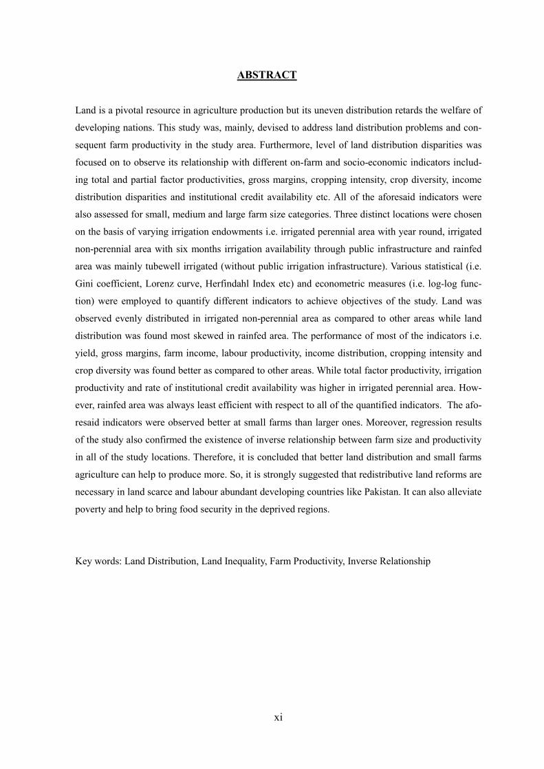
ABSTRACT
Land is a pivotal resource in agriculture production but its uneven distribution retards the welfare of
developing nations. This study was, mainly, devised to address land distribution problems and con-
sequent farm productivity in the study area. Furthermore, level of land distribution disparities was
focused on to observe its relationship with different on-farm and socio-economic indicators includ-
ing total and partial factor productivities, gross margins, cropping intensity, crop diversity, income
distribution disparities and institutional credit availability etc. All of the aforesaid indicators were
also assessed for small, medium and large farm size categories. Three distinct locations were chosen
on the basis of varying irrigation endowments i.e. irrigated perennial area with year round, irrigated
non-perennial area with six months irrigation availability through public infrastructure and rainfed
area was mainly tubewell irrigated (without public irrigation infrastructure). Various statistical (i.e.
Gini coefficient, Lorenz curve, Herfindahl Index etc) and econometric measures (i.e. log-log func-
tion) were employed to quantify different indicators to achieve objectives of the study. Land was
observed evenly distributed in irrigated non-perennial area as compared to other areas while land
distribution was found most skewed in rainfed area. The performance of most of the indicators i.e.
yield, gross margins, farm income, labour productivity, income distribution, cropping intensity and
crop diversity was found better as compared to other areas. While total factor productivity, irrigation
productivity and rate of institutional credit availability was higher in irrigated perennial area. How-
ever, rainfed area was always least efficient with respect to all of the quantified indicators. The afo-
resaid indicators were observed better at small farms than larger ones. Moreover, regression results
of the study also confirmed the existence of inverse relationship between farm size and productivity
in all of the study locations. Therefore, it is concluded that better land distribution and small farms
agriculture can help to produce more. So, it is strongly suggested that redistributive land reforms are
necessary in land scarce and labour abundant developing countries like Pakistan. It can also alleviate
poverty and help to bring food security in the deprived regions.
Key words: Land Distribution, Land Inequality, Farm Productivity, Inverse Relationship
xii
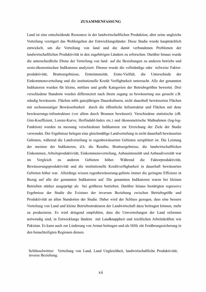
ZUSAMMENFASSUNG
Land ist eine entscheidende Ressource in der landwirtschaftlichen Produktion, aber seine ungleiche
Verteilung verzögert das Wohlergehen der Entwicklungsländer. Diese Studie wurde hauptsächlich
entwickelt, um die Verteilung von land und die damit verbundenen Problemen der
landwirtschaftlichen Produktivität in den zugehörigen Ländern zu erforschen. Darüber hinaus wurde
die unterschiedliche Ebene der Verteilung von land auf die Beziehungen zu anderen betriebs und
sozio-ökonomischen Indikatoren analysiert. Ebenso wurde die vollständige oder teilweise Faktor-
produktivität, Bruttoergebnisse, Ernteintensität, Ernte-Vielfalt, die Unterschiede der
Einkommensverteilung und die institutionelle Kredit Verfügbarkeit untersucht. Alle der genannten
Indikatoren wurden für kleine, mittlere und große Kategorien der Betriebsgrößen bewertet. Drei
verschiedene Standorte wurden differenziert nach ihrem zugang zu bewässerung aus gesucht z.B.
ständig bewässerte. Flächen m0it ganzjährigen Dauerkulturen, nicht dauerhaft bewässerten Flächen
mit sechsmonatiger Bewässerbarkeit durch die öffentliche Infrastruktur und Flächen mit dene
bewässerungs-infrastrukture (vor allem durch Brunnen bewässert). Verschiedene statistische (zB.
Gini-Koeffizient, Lorenz-Kurve, Herfindahl-Index etc.) und ökonometrische Maßnahmen (log-log-
Funktion) wurden zu messung verschiedener Indikatoren zur Erreichung der Ziele der Studie
verwendet. Der Ergebnisse belegen eine gleichmäßige Landverteilung in nicht dauerhaft bewässerten
Gebieten, während die Landverteilung in regenbewässerten Gebieten zersplittert ist. Die Leistung
der meisten der Indikatoren, d.h. die Rendite, Bruttoergebnisse, die landwirtschaftlichen
Einkommen, Arbeitsproduktivität, Einkommensverteilung, Anbauintensität und Anbaudiversität war
im Vergleich zu anderen Gebieten höher. Während die Faktorproduktivität,
Bewässerungsproduktivität und die institutionelle Kreditverfügbarkeit in dauerhaft bewässerten
Gebieten höher war. Allerdings wiesen regenbewässerung-gebiete immer die geringste Effizienz in
Bezug auf alle der genannten Indikatoren auf. Die genannten Indikatoren waren bei kleinen
Betrieben stärker ausgeprägt als bei größeren betrieben. Darüber hinaus bestätigten regressive
Ergebnisse der Studie die Existenz der inversen Beziehung zwischen Betriebsgröße und
Produktivität an allen Standorten der Studie. Daher wird der Schluss gezogen, dass eine bessere
Verteilung von Land und kleine Betriebsstrukturen der Landwirtschaft dazu beitragen können, mehr
zu produzieren. Es wird dringend empfohlen, dass die Umverteilungen der Land reformen
notwendig sind, in Entwicklungs ländern mit Landknappheit und reichlichen Arbeitskräften wie
Pakistan. Es kann auch zur Linderung von Armut beitragen und als Hilfe zür Ernährungssicherung in
den benachteiligten Regionen dienen.
Schlüsselwörter: Verteilung von Land, Land Ungleichheit, landwirtschaftliche Produktivität,
inverse Beziehung.
1
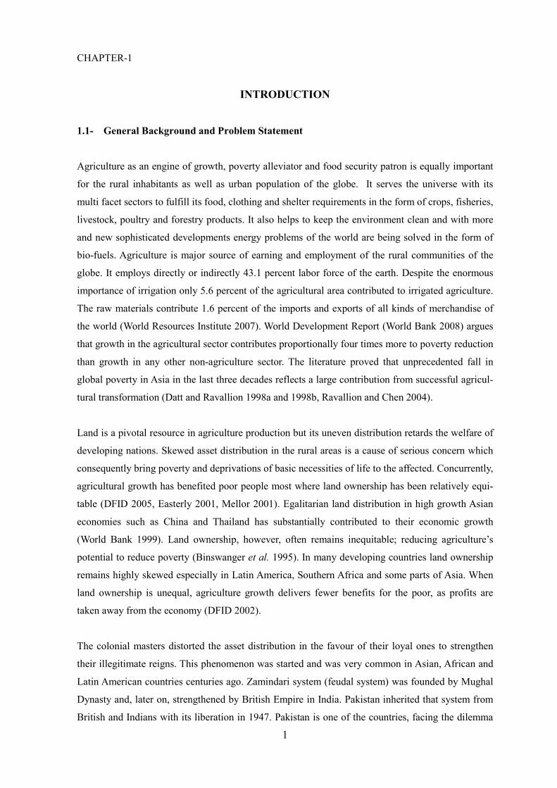
CHAPTER-1
INTRODUCTION
1.1- General Background and Problem Statement
Agriculture as an engine of growth, poverty alleviator and food security patron is equally important
for the rural inhabitants as well as urban population of the globe. It serves the universe with its
multi facet sectors to fulfill its food, clothing and shelter requirements in the form of crops, fisheries,
livestock, poultry and forestry products. It also helps to keep the environment clean and with more
and new sophisticated developments energy problems of the world are being solved in the form of
bio-fuels. Agriculture is major source of earning and employment of the rural communities of the
globe. It employs directly or indirectly 43.1 percent labor force of the earth. Despite the enormous
importance of irrigation only 5.6 percent of the agricultural area contributed to irrigated agriculture.
The raw materials contribute 1.6 percent of the imports and exports of all kinds of merchandise of
the world (World Resources Institute 2007). World Development Report (World Bank 2008) argues
that growth in the agricultural sector contributes proportionally four times more to poverty reduction
than growth in any other non-agriculture sector. The literature proved that unprecedented fall in
global poverty in Asia in the last three decades reflects a large contribution from successful agricul-
tural transformation (Datt and Ravallion 1998a and 1998b, Ravallion and Chen 2004).
Land is a pivotal resource in agriculture production but its uneven distribution retards the welfare of
developing nations. Skewed asset distribution in the rural areas is a cause of serious concern which
consequently bring poverty and deprivations of basic necessities of life to the affected. Concurrently,
agricultural growth has benefited poor people most where land ownership has been relatively equi-
table (DFID 2005, Easterly 2001, Mellor 2001). Egalitarian land distribution in high growth Asian
economies such as China and Thailand has substantially contributed to their economic growth
(World Bank 1999). Land ownership, however, often remains inequitable; reducing agriculture’s
potential to reduce poverty (Binswanger et al. 1995). In many developing countries land ownership
remains highly skewed especially in Latin America, Southern Africa and some parts of Asia. When
land ownership is unequal, agriculture growth delivers fewer benefits for the poor, as profits are
taken away from the economy (DFID 2002).
The colonial masters distorted the asset distribution in the favour of their loyal ones to strengthen
their illegitimate reigns. This phenomenon was started and was very common in Asian, African and
Latin American countries centuries ago. Zamindari system (feudal system) was founded by Mughal
Dynasty and, later on, strengthened by British Empire in India. Pakistan inherited that system from
British and Indians with its liberation in 1947. Pakistan is one of the countries, facing the dilemma
2
of skewed land distribution which could not be resolved despite the three failed land reform attempts
in Pakistan due to overwhelming strength of landlords within the parliament and outside of it. Eighty
one percent farmers own less than 5 hectares in size cover only 38.7 percent of the total farm area.
Furthermore, 6.8 percent farmers hold more than 10 hectares accounting for 39.8 percent of the farm
area (Bhutto and Bazmi 2007). Moreover, 1.4 percent largest farmers occupy 21.2 percent agricul-
tural area of the country. As the land ownership is the sign of prestige and due to the imperfect land
market structure and higher transaction costs poor farmers are unable to purchase land and can not
enhance their asset holding (Heltberg 1998). Nevertheless, neither land reforms efforts nor green
revolution changed significantly the land distribution structure of the country. There was a tempo-
rary downward change in the Gini ratio from 0.62 to 0.51 in 1960 and 1972, respectively. But this
could not persist for longer time and raised continuously from1972 to 2000 (World Bank 2002,
Khan 2006). Skewed land distribution can also be confirmed by Gini coefficient of land ownership
at province level e.g. Punjab had the highest Gini at 0.63 followed by NWFP at 0.59 and Sindh at
0.51 in 2001-02 (Anwar et al. 2004).
Land distribution scenario in Pakistan might have built up a strong conviction about the core prob-
lem. Skewed land distribution is a dilemma which causes lower proportion of land cultivation keep-
ing a vital share of it fallow for years. Though Pakistan is an agricultural economy but, unfortu-
nately, it can not fulfill its food requirements. It has to spend billions of Pakistani Rupees to import
cereals annually. Large agricultural estates cause rural labour force to be unemployed in land scarce
and labour abundant countries like Pakistan. The overall labour productivity is strongly hurt due to
uneven land distribution in agriculture sector. Sense of ownership and matter of survival compel
family workers to strive hard for higher yield per unit area, while hired labour produce less as com-
pared to family worker (Sen 1962 and 1966, Cornia 1985, Unal 2008). The ratio of permanent hired
labour to family labour is only 0.03 in Pakistan (Eastwood et al. 2004). According to some latest
studies, skewed land distribution hampers overall productivity and leads the affected nations towards
underdevelopment (Deininger 2003, FAO 2002, Galor et al. 2005, Galor et al. 2006, Vollrath and
Erickson 2007, Galor and Moav 2004, Easterly and Levine 2003, Galor et al. 2003, Bourguignon
and Verdier 2000, Engerman and Sokoloff 2002, Deininger and Olinto 2000, Sokoloff and Enger-
man 2000, Deininger and Squire 1998, Deininger and Squire 1997, Engerman and Sokoloff 1997)
A significant negative relationship between land inequalities and output per hectare has been empiri-
cally verified (Vollrath 2006). A drop in the Gini coefficient for the size of operational land holdings
of one standard deviation would increase output per hectare by 8.5%. Jeon and Kim (2000) have
documented significant productivity gains from the land reforms undertaken in Korea in 1950s
which limited the amount of land any individual could own. These inequitable land distributions
distort the structure of land size. Therefore, the countries with higher Gini ratios endow a huge area
to a small number of large farms holders and vice versa.
3
Mal-distribution of land draws a segregation line creating two different classes’ i.e. small farmers’
community and elite class with big landed estates. According to Nagayets (2005) Pakistan has large
numbers of small farmers (i.e. 58 %) occupying a little share of land area (i.e. 15 %) like several
other countries around the globe. A bulk of literature supports the hypothesis (i.e. inverse relation-
ship) that small farmers produce more per unit of land than large farmers. Because of its wide-
reaching implications, the inverse relationship between farm size and output is one of the most im-
portant and hotly discussed facts of rural development. This issue is contested one after a pyramid of
research and it is still inconclusive since many decades in agriculture sector.
Enormous evidence shows that rate of rural poverty is higher (Arif 2006,) and it is strongly corre-
lated with lack of assets in rural areas of Pakistan (Anwar et al. 2004). Landless are the absolute
poor while largest farmers are the exception from this phenomenon. Moreover, increase in the size
of land reduces the head count ratio in the poverty trap (Anwar et al. 2004). All of the four provinces
of Pakistan portrays same scenario. In addition, land is used as mortgage weapon to attain institu-
tional credit. As a result, landless farmers or small land holders are disadvantageous groups and they
have to, solely, rely on non institutional credit and their family labour force for cultivation. Above
all, landless as well as smaller farmers are low income groups and they also have to depend upon
nonfarm income to make both ends meet.
Irrigation is amongst one of the most precious resource for agricultural production and plays condu-
cive role to attain better farm output. It is accepted fact that 95 percent of water resources of Paki-
stan are used for agriculture production (Government of Pakistan 2002). Pakistan ranks fifth in the
world and third in Asia in terms of area under irrigated agriculture (Rust et al. 2001). It is com-
prised of more than 80 percent of irrigated agriculture. Irrigated lands are considered as production
friendly due to higher yields per unit area (Bhalla and Roy 1988). Large farmers attain more water
than smaller one due to prevailing rent seeking practices of the public officials and their overwhelm-
ing influence in the area (United Nations 2006). But this aspect i.e. skewed distribution of irrigation
is beyond the scope of the study. Nevertheless, the irrigation productivity gap per hectare on the
small and larger farms is blight for the food security and poverty not only in Pakistan and in other
developing countries as well. Likewise, labor productivity and prevalence of small farms yield gap
between the small and larger farms is a cause of concern.
This study has been, mainly, devised to address land distribution problems and consequent farm
productivity in the study area. Three areas i.e. irrigated perennial area with year round irrigation
from public infrastructure, irrigated non-perennial i.e. with 6 months water availability and rainfed
areas i.e. without public irrigation infrastructure were selected as study sites in district Gujrat and
Mandi Bahauddin of Punjab province of Pakistan. Impacts of land distribution were quantified on
4
farm productivity with many other indicators like irrigation and labour productivities, farm income
and credit availability in each area and overall study area. Land distribution structure, cropping pat-
tern, cropping intensities and crop diversities were also studied in each area as well as at small me-
dium and large farms. The study was found in line with the proponents of the small farms and redis-
tributive land reform promoters on the account of its results. Inequality in ownership holdings was
found skewed in each study location but it was not so profound in case of operational holdings. Land
was observed evenly distributed in irrigated non-perennial area as compared to irrigated perennial
and rainfed areas. It was very interesting to know that better land distribution fostered higher yields
and greater gross margins accompanied by highest farm income and higher cropping intensity and
crop diversity as compared to other areas. Nevertheless, a strong intuition on the strength of ac-
quired results of the study has been developed to put forth the conclusion that even land distribution
can “indeed” reduce poverty and achieve food security. A comparison of various farm sizes was also
undertaken and it was studied whether small farms were less factor investment intensive but more
productive than larger farms in every respect in each area. The study also verified the existence of
“stylized fact of inverse relationship” in each area under study.
1.2- Objectives and Hypothesis of the Study
Three different sites were selected for study with varying characteristics to carry out project with the
ambition to make a small contribution to the economic development literature. This kind of task
always needed some stipulated targets to achieve and in hand information to arrive at destination,
and satisfy curiosity. The study is comprised of two major aspects concerning land resources of agri-
culture production i.e. its distribution and farm size patterns. Moreover, various indicators were
quantified keeping in mind these both facets in various study locations. Therefore, following major
objectives were set to proceed ahead .i.e.
Objectives
1. To gauge land distribution disparities and test its impacts on various indicators of interest i.e.
total and partial factor productivities, cropping intensity, crop diversity, gross margins, in-
come distribution etc in all of the study locations.
2. To explore farm size patterns and quantify the consequent outcomes of total and partial factor
productivities, gross margins, cropping intensity, crop diversity, farm and off farm incomes
etc in each farming system under study.
3. To run regression analysis to see the existence of inverse relationship between farm size and
productivity in overall as well in the various study locations.
5
Hypothesis
1. Land distribution is skewed in overall study area as well as in the various farming systems i.e.
irrigated perennial, irrigated non-perennial and rainfed areas
2. Cropping intensity, crop diversity, total and partial factor productivities (i.e. irrigation and la-
bour productivities), gross margins income distribution etc are higher in evenly land distri-
buted study location as compared to others.
3. All of the aforementioned indicators except labour productivity yield better results at small
farms as compared to other farm size categories in each study location as well as overall
study area.
4. Inverse relationship of farm size and productivity is a valid proposition and it exists in each
study location i.e. irrigated perennial, irrigated non-perennial and rainfed areas under study.
The aforesaid objectives were achieved by employing various mathematical and econometric tools
to know the final results of the study. Land distribution disparity, being one of the major objective,
was quantified by using different tools i.e. quintile method, Lorenz curve and Gini coefficient to
avoid any kind of bias. Moreover, total and partial factor productivities and cropping intensity were
determined by applying various mathematical applications. While Herfindahl index was utilized to
quantify crop diversity in all of the study locations as well as at small, medium and large farm size
categories. In addition, inverse relationship between farm size and productivity was also determined
as an important aspect of study with the help of log-log function. Nonetheless, hypothesis of the
study were tested by using Kruskal Wallis test due to the specific nature of data.
1.3- Organization of the Study
The various components of the work have been presented in dissertation in the following sequence
i.e. i) chapter-2 contains brief introduction of agriculture development in Pakistan since its inde-
pendence (i.e. 1947). It also gives a elegant view of sources of water used in agriculture followed
by post independence land distribution structure and land distribution efforts in form of land reforms
promulgations and their implementation in the country. ii) chapter-3 is comprised of farm and family
characteristics of study area based on empirical data. It also gives an eye view of socio-economics
and agriculture structure of district Gujrat and Mandi Bahauddin because of the fact that the study
site belongs to these both districts. The empirical research area lies within rice-wheat zone of the
Punjab so characteristics of this zone have also been presented in this chapter. iii) In chapter-4, an
6
attempt has been undertaken to present some relevant literature concerning land distribution dispari-
ties and its hazardous impacts on the farming communities and on the society as a whole. This
chapter also contains facts regarding farm size productivity on the basis of previous literature. An
effort has been done to explain the factors affecting farm size productivity in detail. iv) Chapter- 5
describes types of data, study locations, methodology and various data analytical tools utilized in the
study. Furthermore, this chapter also presents hypothesis testing statistical measure as well as
econometric model to observe inverse relationship between farm size and productivity in the study
area. v) Chapter-6 is a pivotal part of this dissertation which contains empirical results of the study.
The results of the study has been arranged in a sequence of land distribution disparity, cropping in-
tensity and diversity, factor productivities, wealth distribution and existence of inverse relationship
in the study area and vi) chapter -7 discusses the results of the study while vii) chapter-8 concludes
the whole study and presents recommendations for policy makers.
1.4- Justification of the study
According to the latest figures the population of Pakistan has risen to 160 million amongst which 34
percent is urban and 66 percent is living in rural areas. A significant portion of rural and urban popu-
lation of Pakistan is suffering from absolute poverty. Agriculture is the single sector of economy
which has highest ratio of beneficiaries with reference to their employment and livelihood. The pre-
carious condition of land distribution structure is not only a great barrier for the agricultural devel-
opment and poverty alleviation but it also affects the efficiency of the rural scarce resources i.e. land
and irrigation. Feudalism and absentee landlordism greatly hampers the agriculture production and
they also distort the whole power structure of rural areas. Due to certain reasons number of small
farmers keep on increasing and crossing subsistence farming limits. Though, small farming is more
productive but subsistence or below subsistence farming can not help the poor to swim out of pov-
erty. Two redistributive land reforms efforts promulgated in 1959 and 1972 could not change the
land distribution structure in the country due to lack of political will and victimization of political
rivals. While land reforms promulgated in 1977 could not be implemented due to military coup in
the country.
This study will help to recognize actual land distribution, land distribution structure, cropping inten-
sity, crop diversity on one hand but on the other side small and larger farms productivity will also be
quantified. On the bigger holdings, absentee landlordism and fallow land practices contribute more
to the miseries of the landless and smaller holders otherwise they can self cultivate free land. In the
end suggestion and policy implication drawn from the study may attract the policy makers to follow
them. Agriculture’s friendly research and development and policies may reduce poverty and guar-
anty food security in Pakistan and in the developing world as well.
7
CHAPTER-2
AGRICULTURE DEVELOPMENT AND ABORTIVE LAND DISTRIBUTION
ATTEMPTS IN PAKISTAN
2.1- Post Independence Agriculture Development in Pakistan
Pakistan is located at 33° 40′ 0″ N, 73° 10′ 0″ E on the globe and it is positioned in arid and semi
arid regions. Its total land area is 307,376 Square miles (796,100 sq km) of which 50 percent is
mountainous terrain, narrow valleys and foothills. The Indus plain where most of irrigated agricul-
ture is located covers about 78,000 sq mile which is almost 25 percent of the total area (Government
of Pakistan 2002a). Agriculture is utilizing 95 percent of the water resources of Pakistan (Govern-
ment of Pakistan 2002) and share 80 percent agricultural outputs from irrigated agriculture
(Chaturvedi 2000, Lipton et al. 2003). Scant and intermittent rainfall plays a complementary role to
support agriculture which is only 240 mm per year (World Bank 2007a).
The population of Pakistan has increased from 33 million at the time of independence in 1947 to
153.95 million in 2005, making it the seventh most populous country in the world. The population
grew at an average rate of 3 percent per annum from 1951 until the mid-1980s. Population growth
slowed to an average rate of 2.6 percent per annum between 1985 and 2000. Since 2000–01 the
country’s population has grown at an annual average rate of almost 2.2 percent The current growth
rate is still high compared with the average population growth of developed and developing coun-
tries which is 0.9 and 1.7 percent, respectively (Government of Pakistan 2005). The human capital in
the rural areas of Pakistan is the lifeline of Pakistani economy which is either skilled or unskilled in
the farm or non-farm sectors of the rural sphere. More than 65 percent of the population of Pakistan
is still rural while a big portion of it i.e. almost 50 percent (women) are professionally inactive.
Agriculture serves as the back bone of Pakistan’s economy. It generates 20.9 percent of its national
income (GDP) and employs 43.4 percent of its labour force and accounts for nearly 9 percent of the
country’s export earnings (Government of Pakistan 2007). Moreover, this sector provides raw mate-
rial to domestic agro-based industries such as sugar, ghee (plant oil), leather and textiles. Most nota-
bly, 65.9 percent of the country’s population living in rural areas depend directly or indirectly on
agriculture for their livelihood (Government of Pakistan 2006). Agricultural growth has historically
played a major role in Pakistan’s development and continues to be crucial for overall growth and
poverty reduction. Table 2.1 shows the historical trends of the real GDP, real agricultural GDP and
population growth since 1960 to 2004. Average annual share of agricultural GDP of Pakistan was
51, 42, 36, 28 and 25 percent in 1950s, 60s, 70s, 80s, and 90s respectively, by employing 68, 64, 58,
8
53, and 50 percent of the labor force of the country (Khan 2006). It has always been source and
pillar of foreign exchange in the form of exports of Pakistan since many decades. Agricultural export
shared 53, 35, 58, 47, 37 and 25 percent of the total export earnings of the Pakistan in 1950-55,
1960-65, 1970-75, 1980-85, 1990-95 and 2000-05 respectively (ibid).
Table-2.1 Agriculture Growth per Capita in Pakistan 1960-2004 (percent)
1960-70 1970-80 1980-90 1990-00 1990-2004
Real GDP Growth 7.19 4.71 6.32 3.75 3.62
Real Ag. GDP Growth 4.89 2.33 4.04 4.42 3.54
Population Growth 2.79 3.18 2.70 2.49 2.47
Rural Population Growth 2.42 2.73 2.34 2.11 2.06
Real Ag. GDP Growth per Capita 2.04 -0.82 1.31 1.88 1.04
Source: World Bank 2007
Even though, agriculture’s share of GDP has fallen from about 40 percent in the 1960s to about 20
percent today. Agriculture remains the largest source of household income for 38 million Pakistanis,
including 13 million of the poorest 40 percent of rural households. However, Substantial scope ex-
ists for increasing productivity and overall economic efficiency in the agriculture sector of Pakistan
(World Bank 2007). Despite progress in GDP and better per hectare yield in the agriculture sector,
the level of rural poverty is quite higher than urban and national averages of the country. It reduced
from 39.1 to 34 percent from 1998-99 to 2004-05 but the figures show that it has continuous increas-
ing trends i.e. 25.2, 25.4, 33.1 and 33.8 in 1990-91, 1993-94, 1996-97 and 1998-99, respectively
(World Bank 2006a , Bhutto and Bazmi 2007). Despite the fluctuations in a tangible to and fro man-
ner of the poverty since decades in the rural areas of Pakistan, agriculture sector has helped the rural
communities to avoid from food insecurity and malnutrition.
The green revolution mechanized Pakistan’s agriculture sector by increasing use of tractors and
tubewells. While high yielding varieties of hybrid seeds and use of chemical fertilizers enhanced
farm efficiency of the country. The green revolution made susceptible to the smaller farmers for
changes that are more resistant to the innovative ideas. It played a crucial role to adopt new tech-
niques and technologies even to the laggards in Pakistan just like other developing countries of the
world. Massive investments in large-scale surface irrigation with the “Indus Basin Waters Treaty”
agreed in 1960 and subsequent major investments in the Tarbela dam (the world’s largest earth-fill
dam) and link canals provided the basis for a vibrant agricultural and the development of the coun-
try’s economy. The worthier development in irrigation sector and advent of green revolution in
1960s boosted agriculture, and capture more and more cultivated land and attracted masses of labor
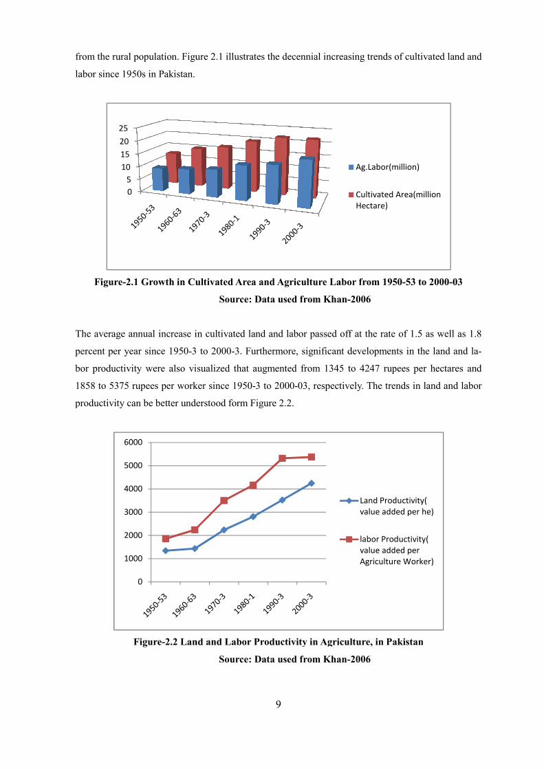
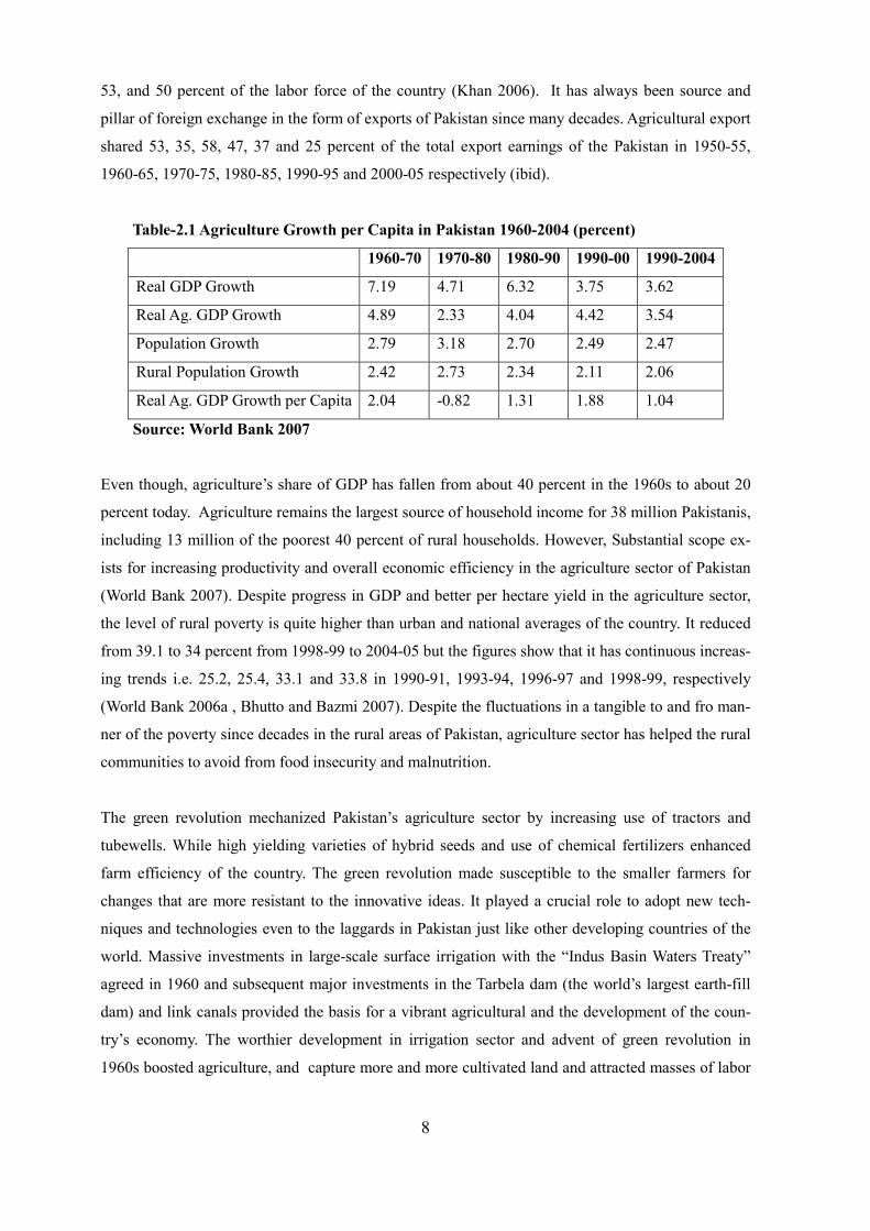
from the rural population. Figure 2.1 illustrates the decennial increasing trends of cultivated la
labor since 1950s in Pakistan.
Figure-2.1 Growth in Cultivated Area and Agriculture Labor from 1950
The average annual increase in cultivated land and labor passed off at the rate of 1.5 as well as
percent per year since 1950-3 to 2000
bor productivity were also visualized that augmented from 1345 to 4247 rupees per hectares and
1858 to 5375 rupees per worker since 1950
productivity can be better understood form Figure 2.2.
Figure-2.2 Land and Labor Productivity in Agriculture, in Pakistan
0
5
10
15
20
25
0
1000
2000
3000
4000
5000
6000
9
from the rural population. Figure 2.1 illustrates the decennial increasing trends of cultivated la
2.1 Growth in Cultivated Area and Agriculture Labor from 1950
Source: Data used from Khan-2006
The average annual increase in cultivated land and labor passed off at the rate of 1.5 as well as
3 to 2000-3. Furthermore, significant developments in the land and l
bor productivity were also visualized that augmented from 1345 to 4247 rupees per hectares and
1858 to 5375 rupees per worker since 1950-3 to 2000-03, respectively. The trends in land and labor
productivity can be better understood form Figure 2.2.
2.2 Land and Labor Productivity in Agriculture, in Pakistan
Source: Data used from Khan-2006
Ag.Labor(million)
Cultivated Area(million
Hectare)
Land Productivity(
value added per he)
labor Productivity(
value added per
Agriculture Worker)
from the rural population. Figure 2.1 illustrates the decennial increasing trends of cultivated land and
2.1 Growth in Cultivated Area and Agriculture Labor from 1950-53 to 2000-03
The average annual increase in cultivated land and labor passed off at the rate of 1.5 as well as 1.8
3. Furthermore, significant developments in the land and la-
bor productivity were also visualized that augmented from 1345 to 4247 rupees per hectares and
ectively. The trends in land and labor
2.2 Land and Labor Productivity in Agriculture, in Pakistan
Ag.Labor(million)
Cultivated Area(million
Land Productivity(
value added per he)
labor Productivity(
value added per
Agriculture Worker)

10
It is evident from the upward trajectory of the figure that both land and labor productivities took
momentum in 1960s with the introduction of green revolution and surface irrigation after Indus ba-
sin treaty with India in 1960.
There are very distinguished two annual crop seasons to grow various major crops called Rabi (win-
ter) and Kharif ( summer) season. Pakistan has been endowed with good climatic conditions to grow
different crops, with the favorable social and economic environment, high potential yield of the
crops can be achieved. Average yield of major crops have almost doubled and in some cases it has
tripled since 1950-3 to 2004-07.
Table-2.2 Average Yield of Major Crops (per hectare)
Year Cotton (Kg) S.Cane ( m-t) Rice (Kg) Wheat (Kg)
1950-3 619 29 879 759
1960-3 732 32 913 824
1970-3 1023 33 1536 1175
1980-3 1041 38 1698 1629
1990-3 1927 42 1556 1926
2000-3 1825 47 1957 2325
2004-07 NA 51 2107 2596
Source: Government of Pakistan 2007 and Khan-2006
It is obvious from table 2.2 that wheat (i.e. staple crop in Pakistan) rose 3.4 times, while rice, cotton
and sugarcane have attained 3, 1.75 and 2.5 times more yield in almost 50 years. Unfortunately, all
these achievements in yields have been dissipated due to higher rate of population growth and vague
public policies. Consequently, Pakistan is suffering from bad wheat shortage these days and is con-
strained to import bulk of it from other countries.
Education plays a pivotal role to learn, organize, integrate and excel the societies and their progress
and prosperity. Unfortunately, achievements in the education sector have been remarkably sluggish
in the rural areas of Pakistan. The backwardness in the literacy rate might be the reason for slower
economic growth and poor rural development of Pakistan. The literacy rate of the rural areas of
Pakistan was mere 17.33 percent in 1981 which rose to 33.64 percent in 1998 (Government of Paki-
stan 1998), and reached ultimately up to 40 percent in 2004-05 (World Bank 2007). Literacy rate in
the rural areas is not very impressive and its progress since last two and half decades is dismal.
11
2.2- Water for Agriculture
It is accepted fact that 95 percent of water resources of Pakistan are used for agriculture production
(Government of Pakistan 2002a). Pakistan ranks fifth in the world and third in Asia in terms of area
under irrigated agriculture (Rust et al. 2001). Pakistan is being irrigated by eminent Indus Basin
irrigation system which is one of the most contiguous systems of the world. The system was de-
signed for 80 percent of cropping intensities i.e. 50 percent during the Kharif season and 30 percent
during the Rabi season (Starkloff and Zaman 1999). The water delivery system, after Indus Basin
treaty with India and consequent construction of network of canals consists of 64,000 Km length to
irrigate over 16 million hectares of land (Rust et al. 2001). Diversion from the Indus river system
and groundwater extraction account for about 60 and 25 percent, respectively, of the annual water
supply for agricultural production. Rainfall in the gross command area accounts for 15 percent of the
total water supply (United Nations 2000). Table 2.3 shows core water resources situation in Paki-
stan.
Table-2.3 Water supplies for Irrigation of the Indus Plan
Sources of Irrigation Volume (MAF*)
Percent
Rainfall 26 14.8
Diversion Canal Irrigation Systems 105 59.6
Ground Water 45 25.6
Total 176 100
Source: United Nations 2000
MAF*= Million Acre Feet
Agriculture in Pakistan is basically irrigated with 82 percent of cultivable area equipped with irriga-
tion infrastructures. During the last 46 years, the area with irrigation facilities increased from 8.21 to
18.0 million ha, at an average annual rate of 1.7 percent. Moreover, most of the increase took place
in canal and tubewell irrigated areas (United Nations 2000). From the total irrigated area (i.e. 19.02
million ha) 7 million ha is canal irrigated, 7.78 million ha is canal plus tubewell irrigated and 3.5
million ha is tubewell irrigated while the rest is irrigated with some other sources (Government of
Pakistan 2005-06). During the era of green revolution Salinity Control Area Reclamation Project
(SCARP) was introduced to the brackish water zone with high water table areas with the help of
World Bank. The ground water is charged with river flow, canal seepage and natural precipitation.
This aquifer, with a potential of about 50 MAF, is being exploited to an extent of about 38 MAF by
over 562,000 private and about 10,000 public tubewells (Kahlow and Majeed 2004). Figure 2.3 ex-
presses the scope of ground water exploitation in Pakistan since 1900.
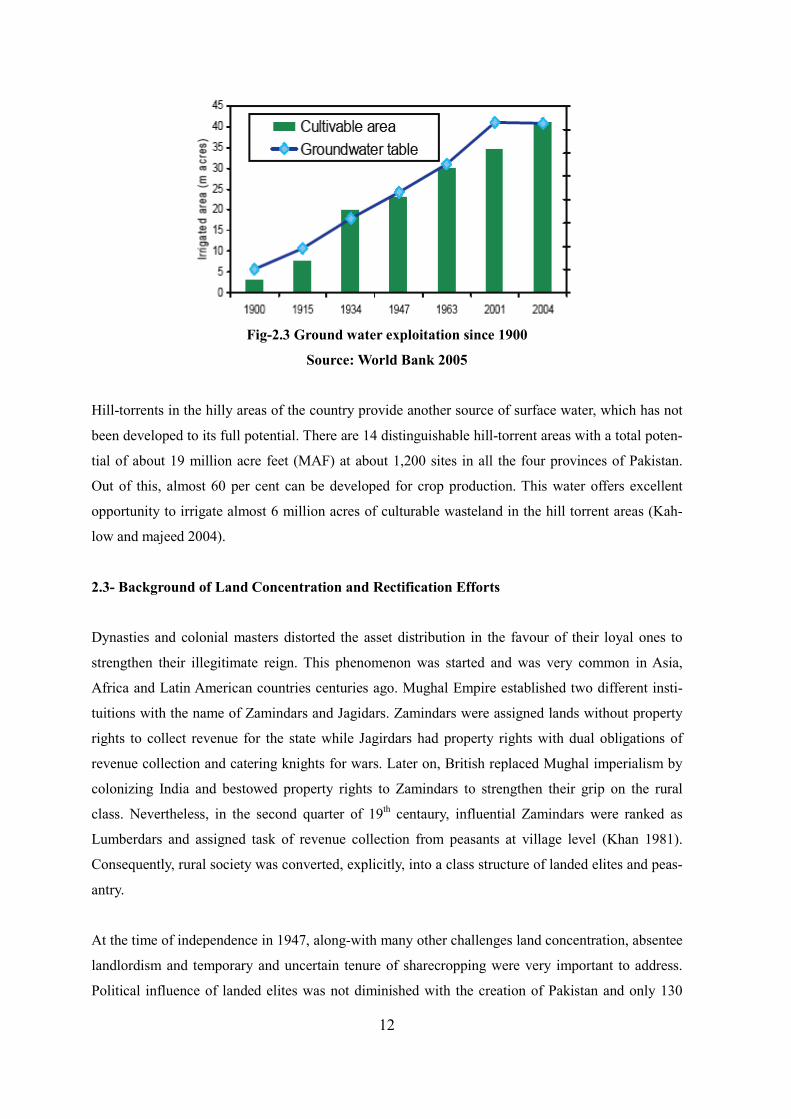
12
Fig-2.3 Ground water exploitation since 1900
Source: World Bank 2005
Hill-torrents in the hilly areas of the country provide another source of surface water, which has not
been developed to its full potential. There are 14 distinguishable hill-torrent areas with a total poten-
tial of about 19 million acre feet (MAF) at about 1,200 sites in all the four provinces of Pakistan.
Out of this, almost 60 per cent can be developed for crop production. This water offers excellent
opportunity to irrigate almost 6 million acres of culturable wasteland in the hill torrent areas (Kah-
low and majeed 2004).
2.3- Background of Land Concentration and Rectification Efforts
Dynasties and colonial masters distorted the asset distribution in the favour of their loyal ones to
strengthen their illegitimate reign. This phenomenon was started and was very common in Asia,
Africa and Latin American countries centuries ago. Mughal Empire established two different insti-
tuitions with the name of Zamindars and Jagidars. Zamindars were assigned lands without property
rights to collect revenue for the state while Jagirdars had property rights with dual obligations of
revenue collection and catering knights for wars. Later on, British replaced Mughal imperialism by
colonizing India and bestowed property rights to Zamindars to strengthen their grip on the rural
class. Nevertheless, in the second quarter of 19th centaury, influential Zamindars were ranked as
Lumberdars and assigned task of revenue collection from peasants at village level (Khan 1981).
Consequently, rural society was converted, explicitly, into a class structure of landed elites and peas-
antry.
At the time of independence in 1947, along-with many other challenges land concentration, absentee
landlordism and temporary and uncertain tenure of sharecropping were very important to address.
Political influence of landed elites was not diminished with the creation of Pakistan and only 130
13
feudals of Sind owned 1.1 million acres of land (Khan 1981). According to Nasr (1996) the Muhajirs
(i.e. migrants from India to Pakistan) first demanded land distribution in 1947 and they had to face a
strong resistance of the landed elites, especially in Sind where the Muhajirs predominated. The
landed elites reacted by appealing to Sindhi nationalism--standing united with their peasants in de-
fending Sind and the rights of sons of soil against the onslaught of migrants.
With the advent of Pakistan in 1949, government started working on the land issues due to its sever-
ity and its long-lasting impacts on the future development of the newly born nation. The “Hari (i.e.
sharecropper) Enquiry Committee” of Sind was established in 1947-48. The committee categorized
two kinds of absentee landlordism i.e. (a) who do not reside on their lands and (b) who reside but do
not take care of their lands. The committee argued that such landlords do not support their tenants
and subjected them to harassment through their intermediaries. Afterwards, the “Muslim League
Agrarian Committee” suggested devolution of Jagirs and to give greater security to tenants in 1949
(Herring 1983). This report was comprised of two parts having full lay out of agrarian reforms. Sub-
sequently land reforms of 1959 and 1972 were designed on the basis of recommendations put forth
by this committee. Consequently, “Sind Tenancy Act of 1950” and “Punjab Protection and Restora-
tion of Tenancy Rights Act of 1950” were promulgated (Khan 1981). Landlords used different tac-
tics to put pressure and avoid from redistributive land reforms as a second step from the govern-
ment. They created dummy shortage of grains in 1952-54 and government had to import from
abroad to fulfill the gap. The worse economic conditions of Pakistan provided opportunity of impos-
ing first Martial Law to a military dictator in 1958. He appointed a land reform commission in the
same month he took over the country. The commission presented their report with consolidated out-
lines which mainly include,
1- Size of individual holdings
2- Resumption of excess land and its distribution
3- Abolition of Jagirs
4- Security for tenants
5- Prevention of fragmentation and consolidation of individual holdings
On the basis these recommendations first land reforms of the country were promulgated in February
1959.
14
2.3.1- Land Reforms 1959
In this part, preconditions and land ceiling, resumption, redistribution of land and achievements of
the reforms regarding land distribution will be briefly discussed.
The regulations were set at the ceiling of 500 acres of irrigated and 1000 acres of un-irrigated lands
(Jalal 1995, Herring 1983, Khan 1981). But some certain exemptions were bestowed to landowners
to keep their land equivalent to 36,000 Produce Index Units (PIU) which was based on pre-
independence revenue settlements (Jalal 1995). The Produce Index Unit (PIU) reflected the measure
of productivity of land according to their type (Hussain 1984). Khan (1981) defined PIU as: any two
different acres of land located separately are assigned the same PIU if they are producing same gross
output in the same year.
Relaxation was also granted on orchards to keep an additional area of 150 (6,000 PIU) acres but not
less than 10 acre block. 18,000 PIU could also be transferred to heirs and 6000 could be gifted to
female family members. Moreover, landowners were allowed to retain area of their choice in com-
pact blocks not less than of an economic holding i.e. 50 acres in Punjab and 64 acres in Sind. How-
ever, the compensation was to be paid on average Rupees 8 per PIU in interest bearing bonds over
25 years which were heritable but not negotiable. The resumed land was to be sold to landless ten-
ants already cultivating and to small farmers to enhance their holding up to 12.5 acres in Punjab and
16 acres in Sind. Furthermore, a part of resumed land was to be sold to other than landless and small
farmers i.e. civil and military servants (Khan 1981).
During the implementation process numbers of declarants were 5,064 but only 15 percent of them
were affected by provision of ceiling on individual land holding. The area of affected declarants was
5.5 million acres of which 27 percent was in Sind and 66 percent in Punjab. Average holding of each
declarant in the country was 7,028 acres but it was an astonishing 11,810 acres in Punjab (Jalal
1995) and 3,765 acres in Sind (Khan 1981).
Jalal (1995) concluded that the lacunae in the land reforms legislation effectively derailed this exer-
cise rather than the process of implementation. A large proportion of the declared land was retained
by the owners which were 66 percent in the country, 71 percent in Punjab and 56 percent in Sind.
Only 1.9 million acres of land was resumed by the government (Khan 1981, Jalal 1995, Bhatia 1990,
Herring 1983), 55 percent from Punjab and 35 percent from Sindh (Khan 1981). While 57 percent of
resumed land was classified as uncultivated (Ibid). Government of Pakistan paid 89.2 million Ru-
pees to former landowners for the resumption of land until 1967 (Jalal 1995).
15
As far as the sale of land is concerned only 50 percent of total resumed was sold until 1967. How-
ever, most of the area was sold to landless and small owners while remaining area was sold to rich
farmers and civil and military officials. Bhatia (1990) said that total 196,000 tenants benefitted from
the sale of resumed land while Herring (1983) mentioned the figure of 150,000 to 2000,000 tenants
with reference to public depart but he greatly suspected it. Moreover, state benefited from the aboli-
tion of the Jagirs in the form of accretion of Rupees 3.1 million of land revenue to the treasury every
year (Bhatia 1990). Many authors criticize the reforms having political motives rather economic and
these were termed as failed land reforms.
2.3.2- Land Reforms 1972
A federal land commission was established, in 1972, to monitor and coordinate between constituted
provincial land commissions and to assist the government in implementing the regulations uniformly
through out the country. Before to promulgate land reforms, the main targets of the reforms which
were to be achieved, were announced on 1st March, 1972. Those were ideal features, if would have
been implanted honestly it might have changed the country into a progressive and prosperous nation
until now. According to Khan (1981) the objectives were as under,
1- New and lower ceiling on individual holdings
2- Resumption of land by the state without compensation
3- Free distribution of land to landless and small peasants
4- Small peasants and landless were exempted to pay for their bought lands during 1959 re-
forms.
5- Restrictions on the evictions of the tenants
6- Consolidation of land holdings
7- Beginnings of programs to create employments for agriculture labourers
While land Reform regulations were promulgated on March 11, 1972 in the reign of Zulfiqar Ali
Bhutto to place ceiling on the agricultural holdings of Pakistan’s large land lords. It was asserted that
the dissolution of Pakistan’s large agricultural holdings would foster a transformation from absentee
16
landlordism to modern agricultural entrepreneurship. Kennedy (1993) elucidated that the rationale
for 1972 land policies were threefold,
• Redistribution of land to the landless would alleviate poverty in the state and would re-
sult in greater equality in rural areas.
• Land reforms would weaken the power and dominance of Pakistan’s feudal class.
• The reforms were crafted to make Pakistan’s agricultural production more efficient.
1972 land reforms were akin to 1959 reforms with reference to individual land ownership rather to
set ceiling at households’ level. However, the ownership ceiling was lower i.e. 150 acres upon irri-
gated and 300 acres on un-irrigated lands as compared to 1959 reforms (Hussain 1984, Kennedy
1993, Nasr 1996, Herring 1983) with the exception to an additional 20 percent of land to the farmers
owning a tractor and tubewell before December 1971, in the form of additional 2000 PIU (Khan
1981, Nasr 1996). But later on, time frame of tractor and tubewell ownership to retain extra units of
land was exempted. Moreover, two main features distinguished these reforms from the previous one.
First, compensation was not given to the affected landlords and second, land was distributed free of
charge to the landless peasants. The exemption of orchards and livestock farms given in 1959 re-
forms was dishonoured. The land owners were allowed to retain area of his choice as long as it was
in compact blocks of not less than 50 acres in Punjab and 64 acres in sind similar to 1959 reforms
regulations. Moreover, due to the understatement of land productivity standard set according to 1940
PIU the actual ceiling in Punjab was 466 and 560 acres in sind for a tractor or tubewell owner (Hus-
sain 1984). The land declared by the landlords circumventing the ceiling, only 42 percent was re-
sumed in Punjab and 59 percent in Sind. The total area resumed by the government was 0.6 million
acres which was far less than the area resumed under 1959 reforms (i.e. 1.9 million acres) (Ibid).
The resumed land was to be allotted free of charge to landless and small peasants. Of the total re-
sumed area, only 308,390 acres of land were allotted to the beneficiaries until 1978 (Khan 1981). In
addition, most of 257,594 acres of resumed land was unfit for cultivation in some regions of Punjab
and sind. According to land commission of Punjab and Sind, a total of 50,548 people benefitted
from the redistribution of land during 1972-78 in these provinces. The average area allotted to each
beneficiary was 5.3 acres in Punjab and 7.9 acres in Sind (Ibid).
1972 land reforms mainly targets opposition leaders and workers in general in all of the provinces
but especially in the provinces of Balochistan and NWFP (North West Frontier Post) (Kenedy 1993).
Both of the land reforms (i.e. promulgated in 1959 and in 1972) were failed to achieve their real
targets even did not reach nearby of them.
17
2.3.3- Post Independence Farm size structure in Pakistan
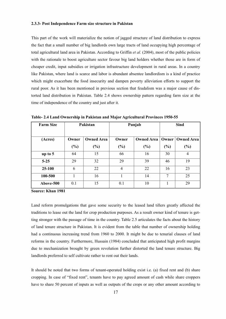
This part of the work will materialize the notion of jagged structure of land distribution to express
the fact that a small number of big landlords own large tracts of land occupying high percentage of
total agricultural land area in Pakistan. According to Griffin et al. (2004), most of the public policies
with the rationale to boost agriculture sector favour big land holders whether those are in form of
cheaper credit, input subsidies or irrigation infrastructure development in rural areas. In a country
like Pakistan, where land is scarce and labor is abundant absentee landlordism is a kind of practice
which might exacerbate the food insecurity and dampen poverty alleviation efforts to support the
rural poor. As it has been mentioned in previous section that feudalism was a major cause of dis-
torted land distribution in Pakistan. Table 2.4 shows ownership pattern regarding farm size at the
time of independence of the country and just after it.
Table- 2.4 Land Ownership in Pakistan and Major Agricultural Provinces 1950-55
Farm Size Pakistan
Punjab
Sind
(Acres) Owner
(%)
Owned Area
(%)
Owner
(%)
Owned Area
(%)
Owner
(%)
Owned Area
(%)
up to 5 64 15 66 16 30 4
5-25 29 32 29 39 46 19
25-100 6 22 4 22 16 23
100-500 1 16 1 14 7 25
Above-500 0.1 15 0.1 10 1 29
Source: Khan 1981
Land reform promulgations that gave some security to the leased land tillers greatly affected the
traditions to lease out the land for crop production purposes. As a result owner kind of tenure is get-
ting stronger with the passage of time in the country. Table 2.5 articulates the facts about the history
of land tenure structure in Pakistan. It is evident from the table that number of ownership holding
had a continuous increasing trend from 1960 to 2000. It might be due to tenurial clauses of land
reforms in the country. Furthermore, Hussain (1984) concluded that anticipated high profit margins
due to mechanization brought by green revolution further distorted the land tenure structure. Big
landlords preferred to self cultivate rather to rent out their lands.
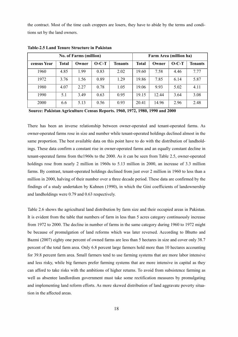
It should be noted that two forms of tenant-operated holding exist i.e. (a) fixed rent and (b) share
cropping. In case of “fixed rent”, tenants have to pay agreed amount of cash while share croppers
have to share 50 percent of inputs as well as outputs of the crops or any other amount according to
18
the contract. Most of the time cash croppers are losers, they have to abide by the terms and condi-
tions set by the land owners.
Table-2.5 Land Tenure Structure in Pakistan
No. of Farms (million) Farm Area (million ha)
census Year Total Owner O-C-T Tenants Total Owner O-C-T Tenants
1960 4.85 1.99 0.83 2.02 19.60 7.58 4.46 7.77
1972 3.76 1.56 0.89 1.29 19.86 7.85 6.14 5.87
1980 4.07 2.27 0.78 1.05 19.06 9.93 5.02 4.11
1990 5.1 3.49 0.63 0.95 19.15 12.44 3.64 3.08
2000 6.6 5.13 0.56 0.93 20.41 14.96 2.96 2.48
Source: Pakistan Agriculture Census Reports. 1960, 1972, 1980, 1990 and 2000
There has been an inverse relationship between owner-operated and tenant-operated farms. As
owner-operated farms rose in size and number while tenant-operated holdings declined almost in the
same proportion. The best available data on this point have to do with the distribution of landhold-
ings. These data confirm a constant rise in owner-operated farms and an equally constant decline in
tenant-operated farms from the1960s to the 2000. As it can be seen from Table 2.5, owner-operated
holdings rose from nearly 2 million in 1960s to 5.13 million in 2000, an increase of 3.3 million
farms. By contrast, tenant-operated holdings declined from just over 2 million in 1960 to less than a
million in 2000, halving of their number over a three decade period. These data are confirmed by the
findings of a study undertaken by Kuhnen (1990), in which the Gini coefficients of landownership
and landholdings were 0.79 and 0.63 respectively.
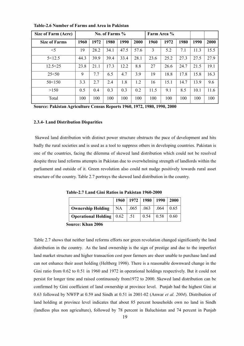
Table 2.6 shows the agricultural land distribution by farm size and their occupied areas in Pakistan.
It is evident from the table that numbers of farm in less than 5 acres category continuously increase
from 1972 to 2000. The decline in number of farms in the same category during 1960 to 1972 might
be because of promulgation of land reforms which was later reversed. According to Bhutto and
Bazmi (2007) eighty one percent of owned farms are less than 5 hectares in size and cover only 38.7
percent of the total farm area. Only 6.8 percent large farmers hold more than 10 hectares accounting
for 39.8 percent farm area. Small farmers tend to use farming systems that are more labor intensive
and less risky, while big farmers prefer farming systems that are more intensive in capital as they
can afford to take risks with the ambitions of higher returns. To avoid from subsistence farming as
well as absentee landlordism government must take some rectification measures by promulgating
and implementing land reform efforts. As more skewed distribution of land aggravate poverty situa-
tion in the affected areas.
19
Table-2.6 Number of Farms and Area in Pakistan
Size of Farm (Acre) No. of Farms % Farm Area %
Size of Farms 1960 1972 1980 1990 2000 1960 1972 1980 1990 2000
<5 19 28.2 34.1 47.5 57.6 3 5.2 7.1 11.3 15.5
5<12.5 44.3 39.9 39.4 33.4 28.1 23.6 25.2 27.3 27.5 27.9
12.5<25 23.8 21.1 17.3 12.2 8.8 27 26.6 24.7 21.5 19.1
25<50 9 7.7 6.5 4.7 3.9 19 18.8 17.8 15.8 16.3
50<150 3.3 2.7 2.4 1.8 1.2 16 15.1 14.7 13.9 9.6
>150 0.5 0.4 0.3 0.3 0.2 11.5 9.1 8.5 10.1 11.6
Total 100 100 100 100 100 100 100 100 100 100
Source: Pakistan Agriculture Census Reports 1960, 1972, 1980, 1990, 2000
2.3.4- Land Distribution Disparities
Skewed land distribution with distinct power structure obstructs the pace of development and hits
badly the rural societies and is used as a tool to suppress others in developing countries. Pakistan is
one of the countries, facing the dilemma of skewed land distribution which could not be resolved
despite three land reforms attempts in Pakistan due to overwhelming strength of landlords within the
parliament and outside of it. Green revolution also could not nudge positively towards rural asset
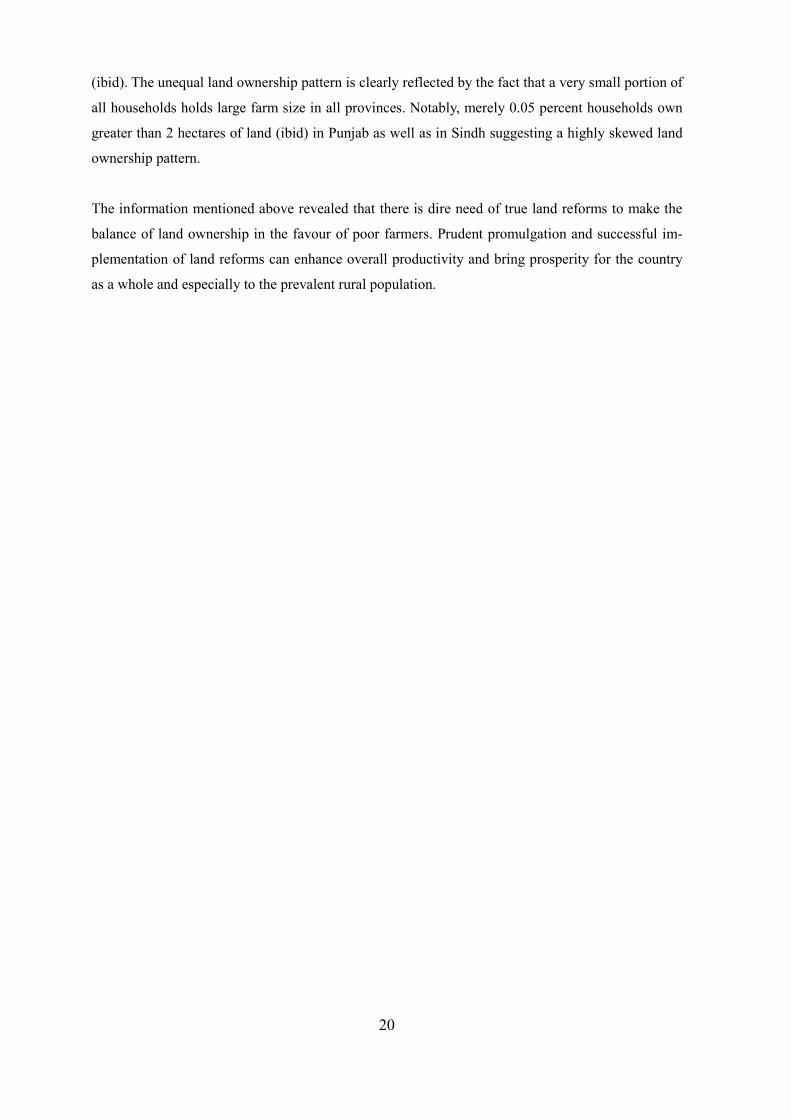
structure of the country. Table 2.7 portrays the skewed land distribution in the country.
Table-2.7 Land Gini Ratios in Pakistan 1960-2000
1960 1972 1980 1990 2000
Ownership Holding NA .065 .063 .064 0.65
Operational Holding 0.62 .51 0.54 0.58 0.60
Source: Khan 2006
Table 2.7 shows that neither land reforms efforts nor green revolution changed significantly the land
distribution in the country. As the land ownership is the sign of prestige and due to the imperfect
land market structure and higher transaction cost poor farmers are sheer unable to purchase land and
can not enhance their asset holding (Heltberg 1998). There is a reasonable downward change in the
Gini ratio from 0.62 to 0.51 in 1960 and 1972 in operational holdings respectively. But it could not
persist for longer time and raised continuously from1972 to 2000. Skewed land distribution can be
confirmed by Gini coefficient of land ownership at province level. Punjab had the highest Gini at
0.63 followed by NWFP at 0.59 and Sindh at 0.51 in 2001-02 (Anwar et al. 2004). Distribution of
land holding at province level indicates that about 85 percent households own no land in Sindh
(landless plus non agriculture), followed by 78 percent in Baluchistan and 74 percent in Punjab
20
(ibid). The unequal land ownership pattern is clearly reflected by the fact that a very small portion of
all households holds large farm size in all provinces. Notably, merely 0.05 percent households own
greater than 2 hectares of land (ibid) in Punjab as well as in Sindh suggesting a highly skewed land
ownership pattern.
The information mentioned above revealed that there is dire need of true land reforms to make the
balance of land ownership in the favour of poor farmers. Prudent promulgation and successful im-
plementation of land reforms can enhance overall productivity and bring prosperity for the country
as a whole and especially to the prevalent rural population.
21
CHAPTER-3
THE STUDY AREA: GENERAL AND FARMING CHARACTERSITICS
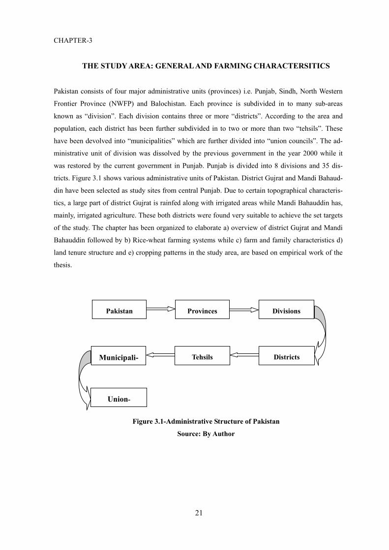
Pakistan consists of four major administrative units (provinces) i.e. Punjab, Sindh, North Western
Frontier Province (NWFP) and Balochistan. Each province is subdivided in to many sub-areas
known as “division”. Each division contains three or more “districts”. According to the area and
population, each district has been further subdivided in to two or more than two “tehsils”. These
have been devolved into “municipalities” which are further divided into “union councils”. The ad-
ministrative unit of division was dissolved by the previous government in the year 2000 while it
was restored by the current government in Punjab. Punjab is divided into 8 divisions and 35 dis-
tricts. Figure 3.1 shows various administrative units of Pakistan. District Gujrat and Mandi Bahaud-
din have been selected as study sites from central Punjab. Due to certain topographical characteris-
tics, a large part of district Gujrat is rainfed along with irrigated areas while Mandi Bahauddin has,
mainly, irrigated agriculture. These both districts were found very suitable to achieve the set targets
of the study. The chapter has been organized to elaborate a) overview of district Gujrat and Mandi
Bahauddin followed by b) Rice-wheat farming systems while c) farm and family characteristics d)
land tenure structure and e) cropping patterns in the study area, are based on empirical work of the
thesis.
Figure 3.1-Administrative Structure of Pakistan
Source: By Author
Municipali-
Pakistan Provinces Divisions
Tehsils Districts
Union-
councils
22
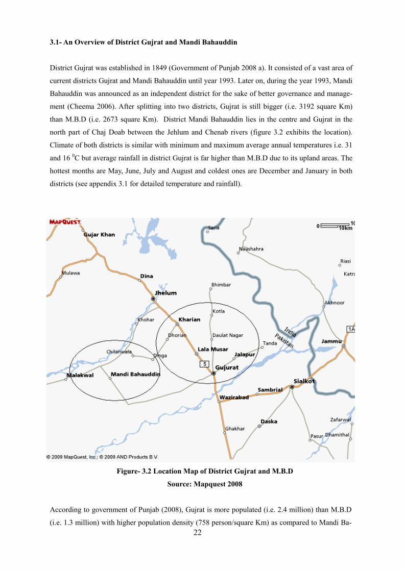
3.1- An Overview of District Gujrat and Mandi Bahauddin
District Gujrat was established in 1849 (Government of Punjab 2008 a). It consisted of a vast area of
current districts Gujrat and Mandi Bahauddin until year 1993. Later on, during the year 1993, Mandi
Bahauddin was announced as an independent district for the sake of better governance and manage-
ment (Cheema 2006). After splitting into two districts, Gujrat is still bigger (i.e. 3192 square Km)
than M.B.D (i.e. 2673 square Km). District Mandi Bahauddin lies in the centre and Gujrat in the
north part of Chaj Doab between the Jehlum and Chenab rivers (figure 3.2 exhibits the location).
Climate of both districts is similar with minimum and maximum average annual temperatures i.e. 31
and 16 0C but average rainfall in district Gujrat is far higher than M.B.D due to its upland areas. The
hottest months are May, June, July and August and coldest ones are December and January in both
districts (see appendix 3.1 for detailed temperature and rainfall).
Figure- 3.2 Location Map of District Gujrat and M.B.D
Source: Mapquest 2008
According to government of Punjab (2008), Gujrat is more populated (i.e. 2.4 million) than M.B.D
(i.e. 1.3 million) with higher population density (758 person/square Km) as compared to Mandi Ba-
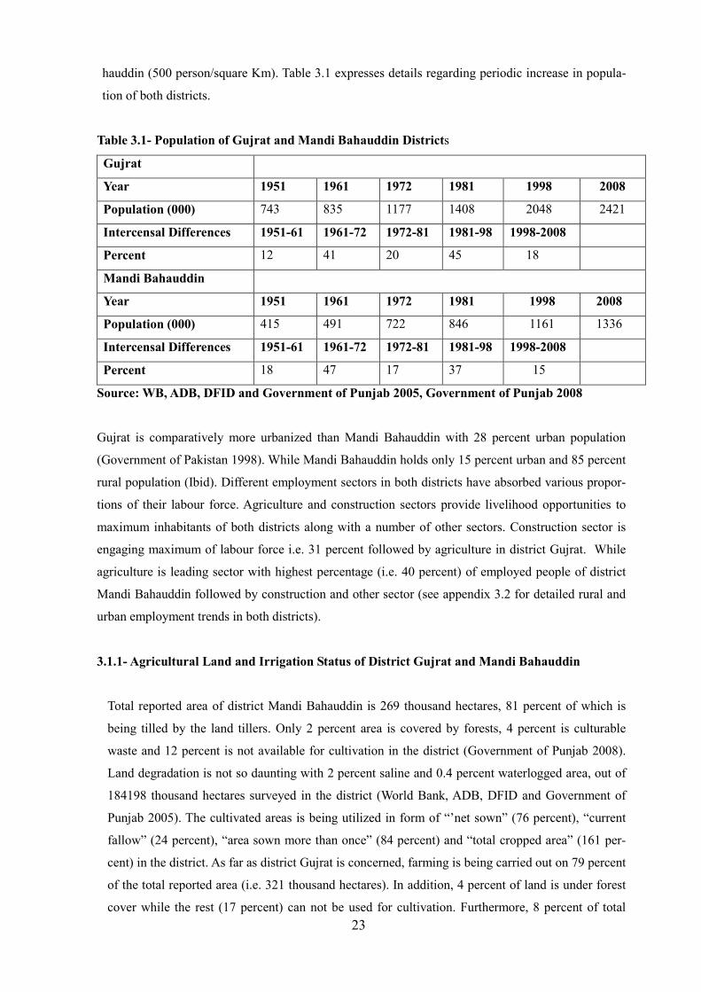
23
hauddin (500 person/square Km). Table 3.1 expresses details regarding periodic increase in popula-
tion of both districts.
Table 3.1- Population of Gujrat and Mandi Bahauddin Districts
Gujrat
Year 1951 1961 1972 1981 1998 2008
Population (000) 743 835 1177 1408 2048 2421
Intercensal Differences 1951-61 1961-72 1972-81 1981-98 1998-2008
Percent 12 41 20 45 18
Mandi Bahauddin
Year 1951 1961 1972 1981 1998 2008
Population (000) 415 491 722 846 1161 1336
Intercensal Differences 1951-61 1961-72 1972-81 1981-98 1998-2008
Percent 18 47 17 37 15
Source: WB, ADB, DFID and Government of Punjab 2005, Government of Punjab 2008
Gujrat is comparatively more urbanized than Mandi Bahauddin with 28 percent urban population
(Government of Pakistan 1998). While Mandi Bahauddin holds only 15 percent urban and 85 percent
rural population (Ibid). Different employment sectors in both districts have absorbed various propor-
tions of their labour force. Agriculture and construction sectors provide livelihood opportunities to
maximum inhabitants of both districts along with a number of other sectors. Construction sector is
engaging maximum of labour force i.e. 31 percent followed by agriculture in district Gujrat. While
agriculture is leading sector with highest percentage (i.e. 40 percent) of employed people of district
Mandi Bahauddin followed by construction and other sector (see appendix 3.2 for detailed rural and
urban employment trends in both districts).
3.1.1- Agricultural Land and Irrigation Status of District Gujrat and Mandi Bahauddin
Total reported area of district Mandi Bahauddin is 269 thousand hectares, 81 percent of which is
being tilled by the land tillers. Only 2 percent area is covered by forests, 4 percent is culturable
waste and 12 percent is not available for cultivation in the district (Government of Punjab 2008).
Land degradation is not so daunting with 2 percent saline and 0.4 percent waterlogged area, out of
184198 thousand hectares surveyed in the district (World Bank, ADB, DFID and Government of
Punjab 2005). The cultivated areas is being utilized in form of “’net sown” (76 percent), “current
fallow” (24 percent), “area sown more than once” (84 percent) and “total cropped area” (161 per-
cent) in the district. As far as district Gujrat is concerned, farming is being carried out on 79 percent
of the total reported area (i.e. 321 thousand hectares). In addition, 4 percent of land is under forest
cover while the rest (17 percent) can not be used for cultivation. Furthermore, 8 percent of total
24
land area is preyed by salinity and 0.16 percent is waterlogged (World Bank, ADB, DFID, and
Government of Punjab 2005). Land utilization statistics show “net sown area” as 91 percent and
the area left fallow was only 9 percent in the whole district. Moreover, 20 percent area was culti-
vated more than once in a year and total “cropped area was 111 percent in the district (Government
of Punjab 2008).
Total irrigated and un-irrigated area in M.B.D district is 98 and 2 percent, respectively. Due to un-
even topography a large area of district Gujrat lacks irrigation infrastructure and, consequently, 49
percent of lands are un-irrigated here (Government of Punjab 2008). Moreover, canal-tubewells and
canal-wells irrigate 75 and 6 percent of sown area while tubewells, canals and wells irrigate 14, 3
and 2 percent sown area in district Mandi Bahauddin. Whereas, major portion of land is being irri-
gated by tubewells followed by canals, canals plus tubewells, canals plus wells and wells in district
Gujrat. Furthermore, these aforementioned modes irrigate 31, 10, 8, 8 and 1 percent of total land
area in the district, respectively. Details regarding land distribution, per capita food production,
food availability and food security regarding both districts have been given at the end (i.e. appendix
3.3, 3.4 and 3.5).
3.2- Farming Systems and the Study Area
Farming System is defined as a population of individual farm systems that have broadly similar re-
source bases, enterprise patterns, household livelihoods and constraints, and for which similar de-
velopment strategies and interventions would be appropriate. Depending on the scale of the analy-
sis, a farming system can encompass a few dozen or many millions of households (Dixon et al.
2001).
Farming system research was initiated in 1970s and some certain criteria were set by the scientists
and, as a result, a number of farming systems were identified in previous decades. Latest farming
system classification was done on the basis of criteria set by Dixon et al. (2001). Seventy two farm-
ing systems has been identified with eight broad and generic categories each in the developing re-
gions. An overview of global farming systems reveals that six irrigated and rice based wetland sys-
tems contain an agricultural population of nearly 900 million. These systems consist of 170 million
hectares of cultivated land of which nearly two thirds are irrigated. There are three major categories
of smallholder rainfed farming systems in humid, highland or dry/cold areas. These different rain-
fed systems altogether comprise of an agricultural population of more than 1.4 billion with 540 mil-
lion ha of cultivated land. Dualistic systems comprise of farms of mixed size contain a further 200
million farm people, with a cultivated area of 11 million ha. Finally, two further minor categories
of smallholder systems i.e. four coastal artisanal fishing-mixed and six urban-based systems con-
tain a combined total of about 100 million people (Dixon and Gulliver 2003).
25
Pakistan has two main cropping seasons i.e. Kharif (winter) and Rabi (summer). Cotton, rice, maize,
sorghum and sugarcane are Kharif crops, while wheat, oilseeds, grams and barley are Rabi crops.
Pickney’s (1989) classification of rural areas into agro-climatic zones is based primarily on the Kharif
crops, because wheat is the predominant crop in the Rabi season virtually in all areas of the country.
He distributed agro ecological zones into 9, with 5 in Punjab, 2 in Sindh, 1 in North-Western Frontier
Post (NWFP) and 1 in Balochistan. While Food and Agriculture Organisation (2004) divided Paki-
stan into 15 tiers with respect to its crop production zones. The irrigated plains of Pakistan constitute
the largest irrigation system in the world, extending from Peshawer valley through the valley of Pun-
jab and Sindh provinces. A number of major cropping systems dominate farming in the irrigated
plains. Almost, every where wheat is the major Rabi crop while major Kharif crops varies depending
on climate, soil and access to market (Byerlee and Hussain-1992). Table 3.2 delineates crop produc-
tion zones in Pakistan explained by FAO (2004) and Khan (2006). Balochistan province with least
agricultural production area of all of the provinces has four agro-climatic zones whereas Sindh and
NWFP, each of them, has 3 while Punjab has 5 zones.
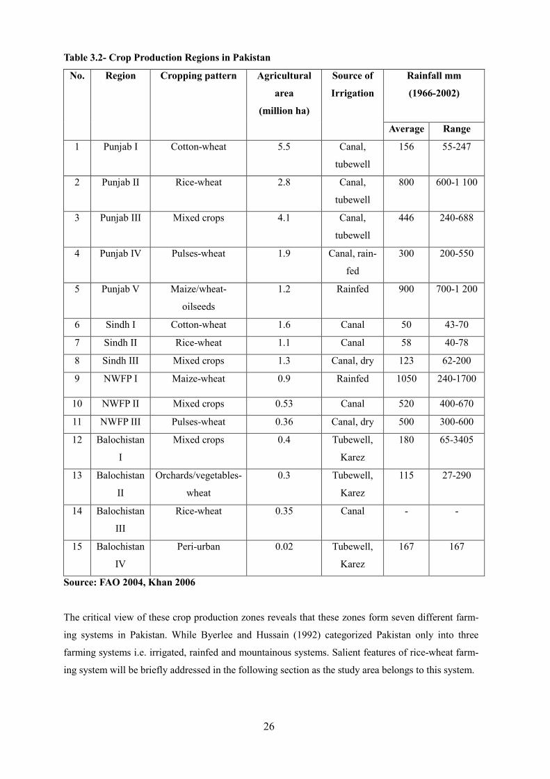
26
Table 3.2- Crop Production Regions in Pakistan
No.
Region
Cropping pattern
Agricultural
area
(million ha)
Source of
Irrigation
Rainfall mm
(1966-2002)
Average Range
1 Punjab I Cotton-wheat 5.5 Canal,
tubewell
156 55-247
2 Punjab II Rice-wheat 2.8 Canal,
tubewell
800 600-1 100
3 Punjab III Mixed crops 4.1 Canal,
tubewell
446 240-688
4 Punjab IV Pulses-wheat 1.9 Canal, rain-
fed
300 200-550
5 Punjab V Maize/wheat-
oilseeds
1.2 Rainfed 900 700-1 200
6 Sindh I Cotton-wheat 1.6 Canal 50 43-70
7 Sindh II Rice-wheat 1.1 Canal 58 40-78
8 Sindh III Mixed crops 1.3 Canal, dry 123 62-200
9 NWFP I Maize-wheat 0.9 Rainfed 1050 240-1700
10 NWFP II Mixed crops 0.53 Canal 520 400-670
11 NWFP III Pulses-wheat 0.36 Canal, dry 500 300-600
12 Balochistan
I
Mixed crops 0.4 Tubewell,
Karez
180 65-3405
13 Balochistan
II
Orchards/vegetables-
wheat
0.3 Tubewell,
Karez
115 27-290
14 Balochistan
III
Rice-wheat 0.35 Canal - -
15 Balochistan
IV
Peri-urban 0.02 Tubewell,
Karez
167 167
Source: FAO 2004, Khan 2006
The critical view of these crop production zones reveals that these zones form seven different farm-
ing systems in Pakistan. While Byerlee and Hussain (1992) categorized Pakistan only into three
farming systems i.e. irrigated, rainfed and mountainous systems. Salient features of rice-wheat farm-
ing system will be briefly addressed in the following section as the study area belongs to this system.
27
3.2.1- Rice Wheat Farming System
In Southeast Asia, the main agro-ecological zones are characterized by humid-subhumid climates,
whilst those in South Asia are arid-semiarid. Irrigated agriculture is well developed in high potential
areas but, with the exception of Pakistan, the countries still depend heavily on rain-fed production
systems (Devendra and Thomas 2002). Amongst the eleven broad farming systems, rice-wheat has
the biggest population and is the second largest land area in South Asian region. It forms a broad
swathe across northern Pakistan in the Indus basin irrigated areas of Sindh and Punjab provinces and
extends up to the northeastern Bangladesh passing through the Indo-Gangetic plains of India. More
than 60 percent land of the area is cultivated and 78 percent of which is irrigated (Dixon et al. 2001).
The study area belongs to irrigated Indus plains and rice-wheat (RW) farming System of Pakistan.
RW farming system is extremely crucial to produce wheat as a staple crop of the country. This sys-
tem occupies 14 percent of irrigated Indus plains of Pakistan and form a core base for national food
grain output (Ahmad et al. 2007). Figure 3.3 shows the location of RW systems in Punjab (2.8 mil-
lion hectares), Sindh (1.1 million hectares), Balochistan (0.35 million hectares) (Khan 2006) and
NWFP provinces of Pakistan. It comprises of six central districts (i.e. Gujrat, Mandi Bahauddin,
Narowal, Sialkot, Gujranwala and Hafizabad) of Punjab province. The climate of RW zone is semi-
arid with long and hot summers lasting from April through September with maximum temperatures
ranging from 21-49 oC and winter lasts December through February with maximum 27
oC day time
temperatures and some time falling below zero at night. The average annual rainfall is 400 mm, 75
percent of which falls during monsoon months i.e. June-September (Ahmad et al. 2007). This area is
famous for quality basmati rice production and contains biggest rice market of Asia.
The large population of RW system is attached with agriculture. Amongst the different categories of
income, share of crop income was 44.5 percent in 2001-2002 (Malik 2003). Moreover, Malik (2003)
reckoned that farm poverty in RW system of Punjab was significantly lower (25 %) than non-farm
(40 percent) households. The facts show that the percentage share of crop income of the overall in-
come rises with increase in number of acreage holding in the area i.e. crop income increase form 23
to 55, 78 and 84 percent with operational holdings up to 1 , 5, 12.5 and more than 12.5 acres per
household, respectively.
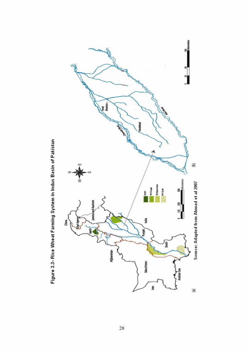
28
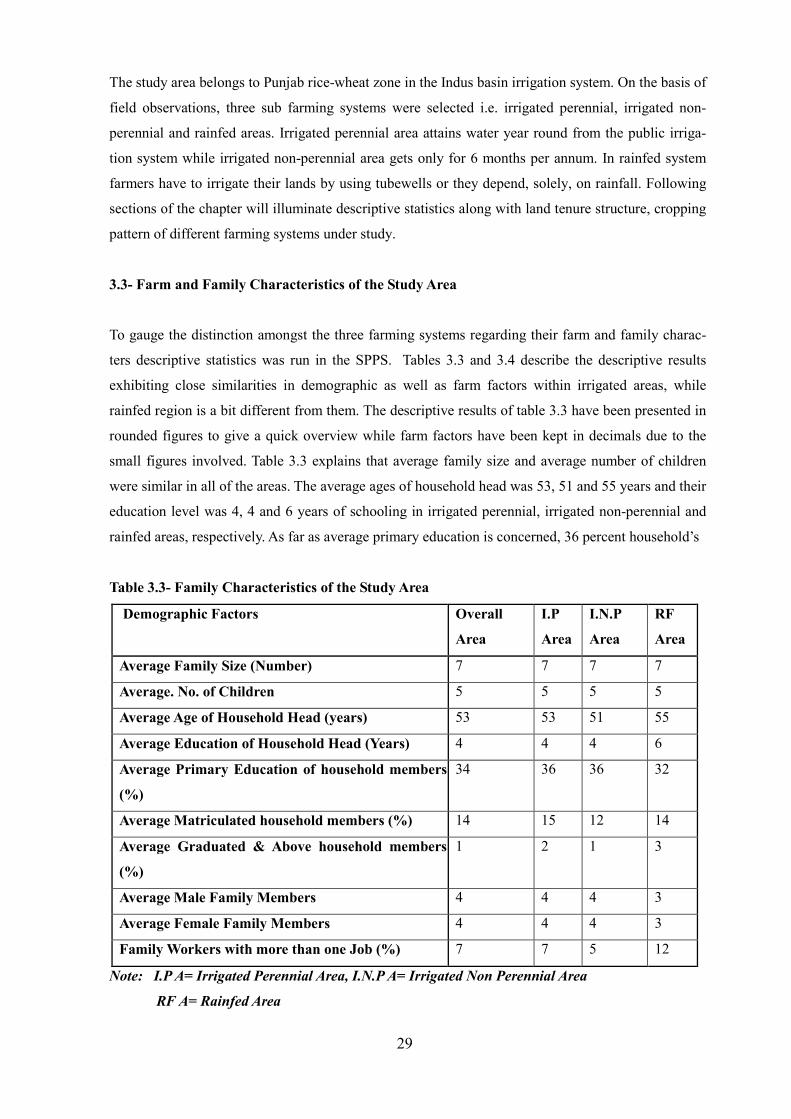
29
The study area belongs to Punjab rice-wheat zone in the Indus basin irrigation system. On the basis of
field observations, three sub farming systems were selected i.e. irrigated perennial, irrigated non-
perennial and rainfed areas. Irrigated perennial area attains water year round from the public irriga-
tion system while irrigated non-perennial area gets only for 6 months per annum. In rainfed system
farmers have to irrigate their lands by using tubewells or they depend, solely, on rainfall. Following
sections of the chapter will illuminate descriptive statistics along with land tenure structure, cropping
pattern of different farming systems under study.
3.3- Farm and Family Characteristics of the Study Area
To gauge the distinction amongst the three farming systems regarding their farm and family charac-
ters descriptive statistics was run in the SPPS. Tables 3.3 and 3.4 describe the descriptive results
exhibiting close similarities in demographic as well as farm factors within irrigated areas, while
rainfed region is a bit different from them. The descriptive results of table 3.3 have been presented in
rounded figures to give a quick overview while farm factors have been kept in decimals due to the
small figures involved. Table 3.3 explains that average family size and average number of children
were similar in all of the areas. The average ages of household head was 53, 51 and 55 years and their
education level was 4, 4 and 6 years of schooling in irrigated perennial, irrigated non-perennial and
rainfed areas, respectively. As far as average primary education is concerned, 36 percent household’s
Table 3.3- Family Characteristics of the Study Area
Demographic Factors Overall
Area
I.P
Area
I.N.P
Area
RF
Area
Average Family Size (Number) 7 7 7 7
Average. No. of Children 5 5 5 5
Average Age of Household Head (years) 53 53 51 55
Average Education of Household Head (Years) 4 4 4 6
Average Primary Education of household members
(%)
34 36 36 32
Average Matriculated household members (%) 14 15 12 14
Average Graduated & Above household members
(%)
1 2 1 3
Average Male Family Members 4 4 4 3
Average Female Family Members 4 4 4 3
Family Workers with more than one Job (%) 7 7 5 12
Note: I.P A= Irrigated Perennial Area, I.N.P A= Irrigated Non Perennial Area
RF A= Rainfed Area
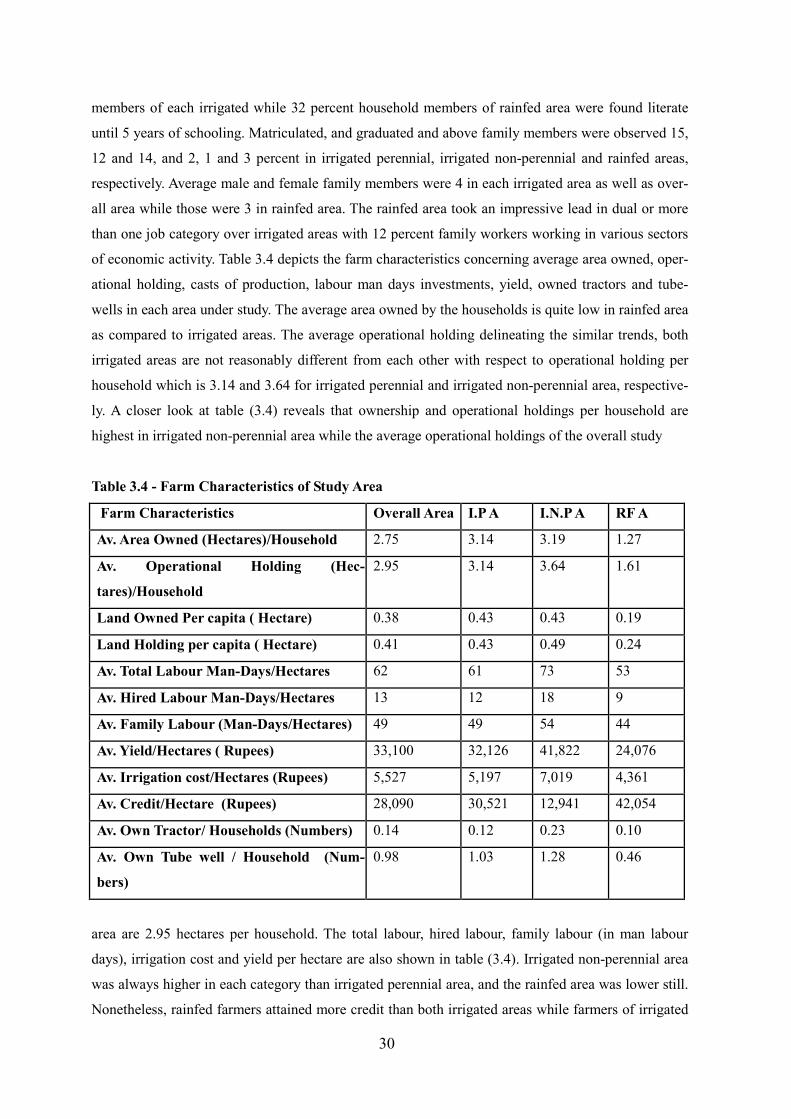
30
members of each irrigated while 32 percent household members of rainfed area were found literate
until 5 years of schooling. Matriculated, and graduated and above family members were observed 15,
12 and 14, and 2, 1 and 3 percent in irrigated perennial, irrigated non-perennial and rainfed areas,
respectively. Average male and female family members were 4 in each irrigated area as well as over-
all area while those were 3 in rainfed area. The rainfed area took an impressive lead in dual or more
than one job category over irrigated areas with 12 percent family workers working in various sectors
of economic activity. Table 3.4 depicts the farm characteristics concerning average area owned, oper-
ational holding, casts of production, labour man days investments, yield, owned tractors and tube-
wells in each area under study. The average area owned by the households is quite low in rainfed area
as compared to irrigated areas. The average operational holding delineating the similar trends, both
irrigated areas are not reasonably different from each other with respect to operational holding per
household which is 3.14 and 3.64 for irrigated perennial and irrigated non-perennial area, respective-
ly. A closer look at table (3.4) reveals that ownership and operational holdings per household are
highest in irrigated non-perennial area while the average operational holdings of the overall study
Table 3.4 - Farm Characteristics of Study Area
Farm Characteristics Overall Area I.P A I.N.P A RF A
Av. Area Owned (Hectares)/Household 2.75 3.14 3.19 1.27
Av. Operational Holding (Hec-
tares)/Household
2.95 3.14 3.64 1.61
Land Owned Per capita ( Hectare) 0.38 0.43 0.43 0.19
Land Holding per capita ( Hectare) 0.41 0.43 0.49 0.24
Av. Total Labour Man-Days/Hectares 62 61 73 53
Av. Hired Labour Man-Days/Hectares 13 12 18 9
Av. Family Labour (Man-Days/Hectares) 49 49 54 44
Av. Yield/Hectares ( Rupees) 33,100 32,126 41,822 24,076
Av. Irrigation cost/Hectares (Rupees) 5,527 5,197 7,019 4,361
Av. Credit/Hectare (Rupees) 28,090 30,521 12,941 42,054
Av. Own Tractor/ Households (Numbers) 0.14 0.12 0.23 0.10
Av. Own Tube well / Household (Num-
bers)
0.98 1.03 1.28 0.46
area are 2.95 hectares per household. The total labour, hired labour, family labour (in man labour
days), irrigation cost and yield per hectare are also shown in table (3.4). Irrigated non-perennial area
was always higher in each category than irrigated perennial area, and the rainfed area was lower still.
Nonetheless, rainfed farmers attained more credit than both irrigated areas while farmers of irrigated
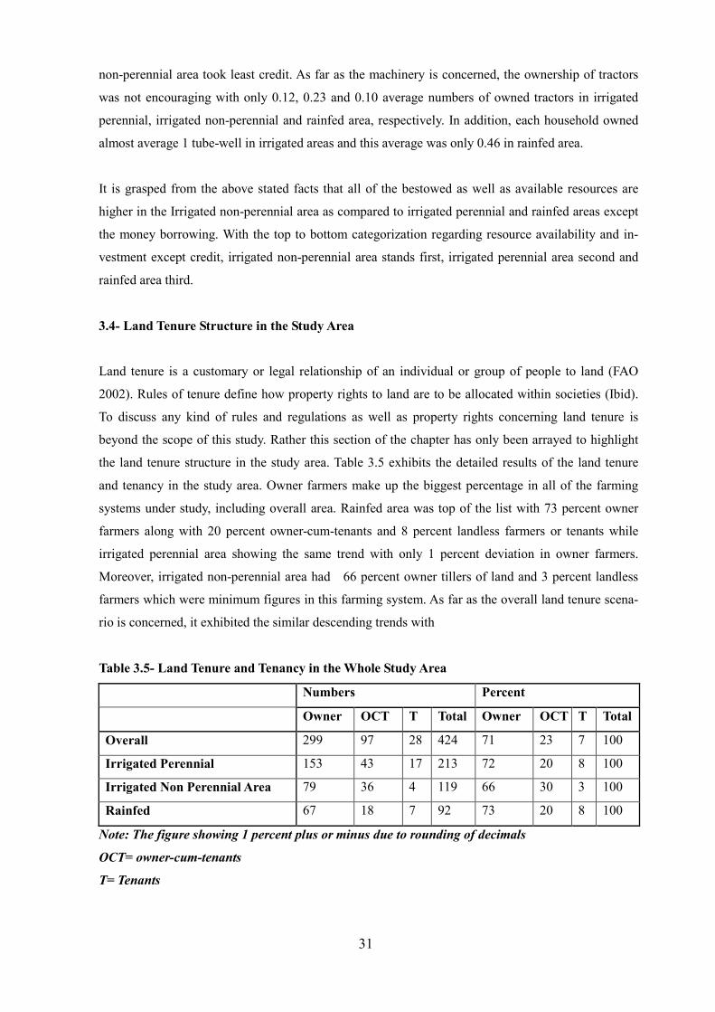
31
non-perennial area took least credit. As far as the machinery is concerned, the ownership of tractors
was not encouraging with only 0.12, 0.23 and 0.10 average numbers of owned tractors in irrigated
perennial, irrigated non-perennial and rainfed area, respectively. In addition, each household owned
almost average 1 tube-well in irrigated areas and this average was only 0.46 in rainfed area.
It is grasped from the above stated facts that all of the bestowed as well as available resources are
higher in the Irrigated non-perennial area as compared to irrigated perennial and rainfed areas except
the money borrowing. With the top to bottom categorization regarding resource availability and in-
vestment except credit, irrigated non-perennial area stands first, irrigated perennial area second and
rainfed area third.
3.4- Land Tenure Structure in the Study Area
Land tenure is a customary or legal relationship of an individual or group of people to land (FAO
2002). Rules of tenure define how property rights to land are to be allocated within societies (Ibid).
To discuss any kind of rules and regulations as well as property rights concerning land tenure is
beyond the scope of this study. Rather this section of the chapter has only been arrayed to highlight
the land tenure structure in the study area. Table 3.5 exhibits the detailed results of the land tenure
and tenancy in the study area. Owner farmers make up the biggest percentage in all of the farming
systems under study, including overall area. Rainfed area was top of the list with 73 percent owner
farmers along with 20 percent owner-cum-tenants and 8 percent landless farmers or tenants while
irrigated perennial area showing the same trend with only 1 percent deviation in owner farmers.
Moreover, irrigated non-perennial area had 66 percent owner tillers of land and 3 percent landless
farmers which were minimum figures in this farming system. As far as the overall land tenure scena-
rio is concerned, it exhibited the similar descending trends with
Table 3.5- Land Tenure and Tenancy in the Whole Study Area
Numbers Percent
Owner OCT T Total Owner OCT T Total
Overall 299 97 28 424 71 23 7 100
Irrigated Perennial 153 43 17 213 72 20 8 100
Irrigated Non Perennial Area 79 36 4 119 66 30 3 100
Rainfed 67 18 7 92 73 20 8 100
Note: The figure showing 1 percent plus or minus due to rounding of decimals
OCT= owner-cum-tenants
T= Tenants
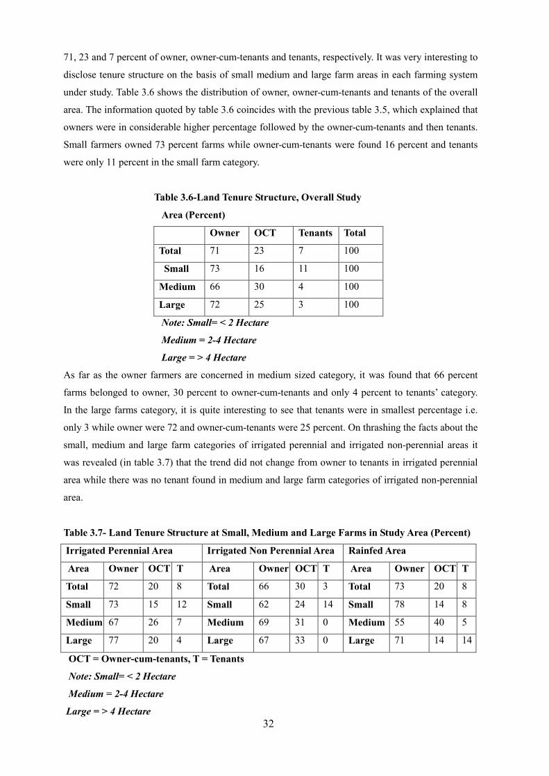
32
71, 23 and 7 percent of owner, owner-cum-tenants and tenants, respectively. It was very interesting to
disclose tenure structure on the basis of small medium and large farm areas in each farming system
under study. Table 3.6 shows the distribution of owner, owner-cum-tenants and tenants of the overall
area. The information quoted by table 3.6 coincides with the previous table 3.5, which explained that
owners were in considerable higher percentage followed by the owner-cum-tenants and then tenants.
Small farmers owned 73 percent farms while owner-cum-tenants were found 16 percent and tenants
were only 11 percent in the small farm category.
Table 3.6-Land Tenure Structure, Overall Study
Area (Percent)
Owner OCT Tenants Total
Total 71 23 7 100
Small 73 16 11 100
Medium 66 30 4 100
Large 72 25 3 100
Note: Small= < 2 Hectare
Medium = 2-4 Hectare
Large = > 4 Hectare
As far as the owner farmers are concerned in medium sized category, it was found that 66 percent
farms belonged to owner, 30 percent to owner-cum-tenants and only 4 percent to tenants’ category.
In the large farms category, it is quite interesting to see that tenants were in smallest percentage i.e.
only 3 while owner were 72 and owner-cum-tenants were 25 percent. On thrashing the facts about the
small, medium and large farm categories of irrigated perennial and irrigated non-perennial areas it
was revealed (in table 3.7) that the trend did not change from owner to tenants in irrigated perennial
area while there was no tenant found in medium and large farm categories of irrigated non-perennial
area.
Table 3.7- Land Tenure Structure at Small, Medium and Large Farms in Study Area (Percent)
Irrigated Perennial Area Irrigated Non Perennial Area Rainfed Area
Area Owner OCT T Area Owner OCT T Area Owner OCT T
Total 72 20 8 Total 66 30 3 Total 73 20 8
Small 73 15 12 Small 62 24 14 Small 78 14 8
Medium 67 26 7 Medium 69 31 0 Medium 55 40 5
Large 77 20 4 Large 67 33 0 Large 71 14 14
OCT = Owner-cum-tenants, T = Tenants
Note: Small= < 2 Hectare
Medium = 2-4 Hectare
Large = > 4 Hectare
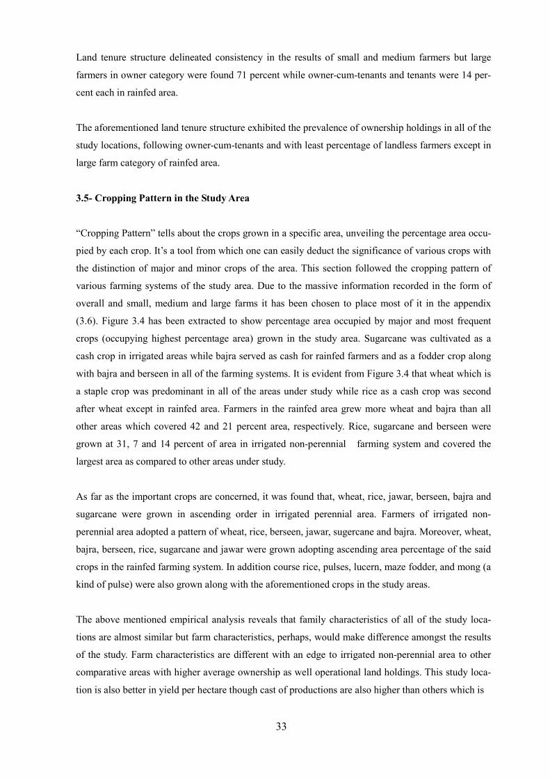
33
Land tenure structure delineated consistency in the results of small and medium farmers but large
farmers in owner category were found 71 percent while owner-cum-tenants and tenants were 14 per-
cent each in rainfed area.
The aforementioned land tenure structure exhibited the prevalence of ownership holdings in all of the
study locations, following owner-cum-tenants and with least percentage of landless farmers except in
large farm category of rainfed area.
3.5- Cropping Pattern in the Study Area
“Cropping Pattern” tells about the crops grown in a specific area, unveiling the percentage area occu-
pied by each crop. It’s a tool from which one can easily deduct the significance of various crops with
the distinction of major and minor crops of the area. This section followed the cropping pattern of
various farming systems of the study area. Due to the massive information recorded in the form of
overall and small, medium and large farms it has been chosen to place most of it in the appendix
(3.6). Figure 3.4 has been extracted to show percentage area occupied by major and most frequent
crops (occupying highest percentage area) grown in the study area. Sugarcane was cultivated as a
cash crop in irrigated areas while bajra served as cash for rainfed farmers and as a fodder crop along
with bajra and berseen in all of the farming systems. It is evident from Figure 3.4 that wheat which is
a staple crop was predominant in all of the areas under study while rice as a cash crop was second
after wheat except in rainfed area. Farmers in the rainfed area grew more wheat and bajra than all
other areas which covered 42 and 21 percent area, respectively. Rice, sugarcane and berseen were
grown at 31, 7 and 14 percent of area in irrigated non-perennial farming system and covered the
largest area as compared to other areas under study.
As far as the important crops are concerned, it was found that, wheat, rice, jawar, berseen, bajra and
sugarcane were grown in ascending order in irrigated perennial area. Farmers of irrigated non-
perennial area adopted a pattern of wheat, rice, berseen, jawar, sugercane and bajra. Moreover, wheat,
bajra, berseen, rice, sugarcane and jawar were grown adopting ascending area percentage of the said
crops in the rainfed farming system. In addition course rice, pulses, lucern, maze fodder, and mong (a
kind of pulse) were also grown along with the aforementioned crops in the study areas.
The above mentioned empirical analysis reveals that family characteristics of all of the study loca-
tions are almost similar but farm characteristics, perhaps, would make difference amongst the results
of the study. Farm characteristics are different with an edge to irrigated non-perennial area to other
comparative areas with higher average ownership as well operational land holdings. This study loca-
tion is also better in yield per hectare though cast of productions are also higher than others which is
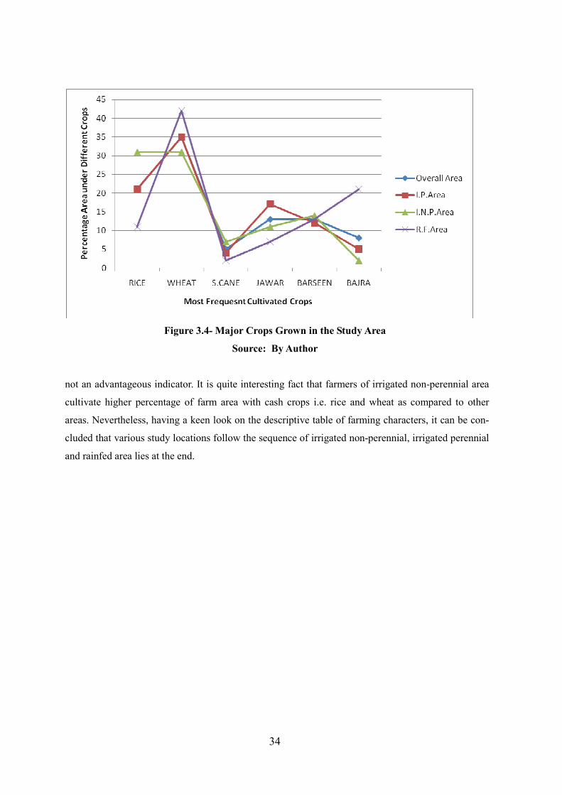
34
Figure 3.4- Major Crops Grown in the Study Area
Source: By Author
not an advantageous indicator. It is quite interesting fact that farmers of irrigated non-perennial area
cultivate higher percentage of farm area with cash crops i.e. rice and wheat as compared to other
areas. Nevertheless, having a keen look on the descriptive table of farming characters, it can be con-
cluded that various study locations follow the sequence of irrigated non-perennial, irrigated perennial
and rainfed area lies at the end.
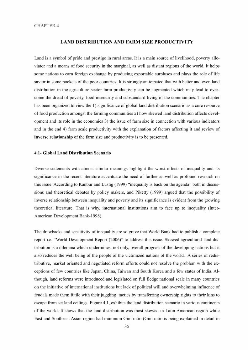
35
CHAPTER-4
LAND DISTRIBUTION AND FARM SIZE PRODUCTIVITY
Land is a symbol of pride and prestige in rural areas. It is a main source of livelihood, poverty alle-
viator and a means of food security in the marginal, as well as distant regions of the world. It helps
some nations to earn foreign exchange by producing exportable surpluses and plays the role of life
savior in some pockets of the poor countries. It is strongly anticipated that with better and even land
distribution in the agriculture sector farm productivity can be augmented which may lead to over-
come the dread of poverty, food insecurity and substandard living of the communities. The chapter
has been organized to view the 1) significance of global land distribution scenario as a core resource
of food production amongst the farming communities 2) how skewed land distribution affects devel-
opment and its role in the economies 3) the issue of farm size in connection with various indicators
and in the end 4) farm scale productivity with the explanation of factors affecting it and review of
inverse relationship of the farm size and productivity is to be presented.
4.1- Global Land Distribution Scenario
Diverse statements with almost similar meanings highlight the worst effects of inequality and its
significance in the recent literature accentuate the need of further as well as profound research on
this issue. According to Kanbur and Lustig (1999) “inequality is back on the agenda” both in discus-
sions and theoretical debates by policy makers, and Piketty (1999) argued that the possibility of
inverse relationship between inequality and poverty and its significance is evident from the growing
theoretical literature. That is why, international institutions aim to face up to inequality (Inter-
American Development Bank-1998).
The drawbacks and sensitivity of inequality are so grave that World Bank had to publish a complete
report i.e. “World Development Report (2006)” to address this issue. Skewed agricultural land dis-
tribution is a dilemma which undermines, not only, overall progress of the developing nations but it
also reduces the well being of the people of the victimized nations of the world. A series of redis-
tributive, market oriented and negotiated reform efforts could not resolve the problem with the ex-
ceptions of few countries like Japan, China, Taiwan and South Korea and a few states of India. Al-
though, land reforms were introduced and legislated on full fledge national scale in many countries
on the initiative of international institutions but lack of political will and overwhelming influence of
feudals made them futile with their juggling tactics by transferring ownership rights to their kins to
escape from set land ceilings. Figure 4.1, exhibits the land distribution scenario in various continents
of the world. It shows that the land distribution was most skewed in Latin American region while
East and Southeast Asian region had minimum Gini ratio (Gini ratio is being explained in detail in
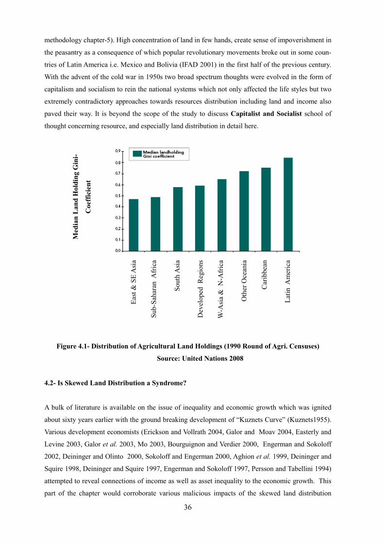
36
methodology chapter-5). High concentration of land in few hands, create sense of impoverishment in
the peasantry as a consequence of which popular revolutionary movements broke out in some coun-
tries of Latin America i.e. Mexico and Bolivia (IFAD 2001) in the first half of the previous century.
With the advent of the cold war in 1950s two broad spectrum thoughts were evolved in the form of
capitalism and socialism to rein the national systems which not only affected the life styles but two
extremely contradictory approaches towards resources distribution including land and income also
paved their way. It is beyond the scope of the study to discuss Capitalist and Socialist school of
thought concerning resource, and especially land distribution in detail here.
Median Land Holding Gini-
Coefficient
Eas
t &
SE
Asi
a
Sub
-Sah
aran
Afr
ica
South
Asi
a
Dev
eloped
R
egio
ns
W-A
sia
& N
-Afr
ica
Oth
er O
cean
ia
Car
ibbea
n
Lat
in A
mer
ica
Figure 4.1- Distribution of Agricultural Land Holdings (1990 Round of Agri. Censuses)
Source: United Nations 2008
4.2- Is Skewed Land Distribution a Syndrome?
A bulk of literature is available on the issue of inequality and economic growth which was ignited
about sixty years earlier with the ground breaking development of “Kuznets Curve” (Kuznets1955).
Various development economists (Erickson and Vollrath 2004, Galor and Moav 2004, Easterly and
Levine 2003, Galor et al. 2003, Mo 2003, Bourguignon and Verdier 2000, Engerman and Sokoloff
2002, Deininger and Olinto 2000, Sokoloff and Engerman 2000, Aghion et al. 1999, Deininger and
Squire 1998, Deininger and Squire 1997, Engerman and Sokoloff 1997, Persson and Tabellini 1994)
attempted to reveal connections of income as well as asset inequality to the economic growth. This
part of the chapter would corroborate various malicious impacts of the skewed land distribution
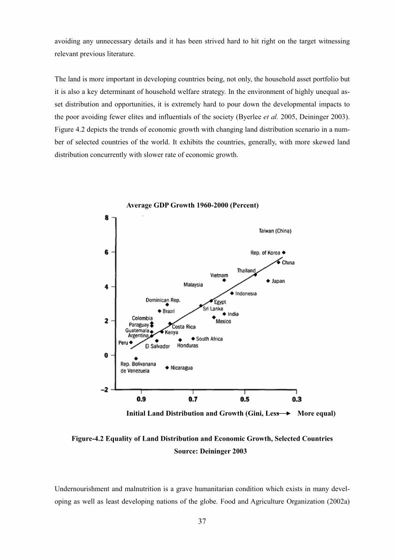
37
avoiding any unnecessary details and it has been strived hard to hit right on the target witnessing
relevant previous literature.
The land is more important in developing countries being, not only, the household asset portfolio but
it is also a key determinant of household welfare strategy. In the environment of highly unequal as-
set distribution and opportunities, it is extremely hard to pour down the developmental impacts to
the poor avoiding fewer elites and influentials of the society (Byerlee et al. 2005, Deininger 2003).
Figure 4.2 depicts the trends of economic growth with changing land distribution scenario in a num-
ber of selected countries of the world. It exhibits the countries, generally, with more skewed land
distribution concurrently with slower rate of economic growth.
Average GDP Growth 1960-2000 (Percent)
Initial Land Distribution and Growth (Gini, Less More equal)
Figure-4.2 Equality of Land Distribution and Economic Growth, Selected Countries
Source: Deininger 2003
Undernourishment and malnutrition is a grave humanitarian condition which exists in many devel-
oping as well as least developing nations of the globe. Food and Agriculture Organization (2002a)
38
considers skewed land distribution as one of the major causes of undernourishment of human popu-
lation along with some other reasons. Figure 4.3 delineates status of undernourishment in connection
with level of land distribution disparities within various developing countries.
Figure-4.3 Impact of Skewed Land Distribution on Undernourishment
Source: FAO 2002a
Land distribution pattern, either skewed or better distributed, played a crucial role in transition of
agrarian economies to industrial ones. Abundance of land was pivotal in early stages of development
while it posed serious hurdle in later phases in the accumulation of human capital and economic
growth in the countries in which the land was unequally distributed. Some of the land abundant
countries considered as rich nations like many Latin American countries in the pre-industrial era
were overtaken by the scarce land nations in which the land was, rather, comparatively better dis-
tributed. Though United States and Canada were land abundant countries like Latin American coun-
tries but those had relatively egalitarian land distribution unlike of concentrated land in a few hands
only. Even land distribution in North American countries made them capable of to invest better in
human capital as compared to Latin Americans (Galor et al. 2005). The same group of authors (Ga-
lor et al. 2006) in another publication discussed the repercussion of unequal distribution of land
ownership on human capital promoting institutions. Cross state public investment on education was
studied keeping in view the unequal land ownership in United States in the early 20th century. It was
concluded that public expenditures on education promoting institutions were inversely related as it is
evident from figure (4.4) which depicts the public expenditures and Gini of Land on Y and X axis
respectively.
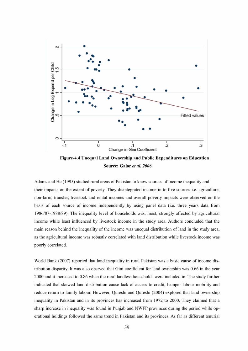
39
Figure-4.4 Unequal Land Ownership and Public Expenditures on Education
Source: Galor et al. 2006
Adams and He (1995) studied rural areas of Pakistan to know sources of income inequality and
their impacts on the extent of poverty. They disintegrated income in to five sources i.e. agriculture,
non-farm, transfer, livestock and rental incomes and overall poverty impacts were observed on the
basis of each source of income independently by using panel data (i.e. three years data from
1986/87-1988/89). The inequality level of households was, most, strongly affected by agricultural
income while least influenced by livestock income in the study area. Authors concluded that the
main reason behind the inequality of the income was unequal distribution of land in the study area,
as the agricultural income was robustly correlated with land distribution while livestock income was
poorly correlated.
World Bank (2007) reported that land inequality in rural Pakistan was a basic cause of income dis-
tribution disparity. It was also obsrved that Gini coefficient for land ownership was 0.66 in the year
2000 and it increased to 0.86 when the rural landless households were included in. The study further
indicated that skewed land distribution cause lack of access to credit, hamper labour mobility and
reduce return to family labour. However, Qureshi and Qureshi (2004) explored that land ownership
inequality in Pakistan and in its provinces has increased from 1972 to 2000. They claimed that a
sharp increase in inequality was found in Punjab and NWFP provinces during the period while op-
erational holdings followed the same trend in Pakistan and its provinces. As far as different tenurial
40
classes are concerned they said that the distribution of farm area among farms of various sizes has
been more unequal under owner operated category of farmers.
In a comparative study of five African countries (i.e. Ethiopia, Kenya, Rwanda, Mozambique, and
Zambia) Jayne et al. (2003) explored relationship between household per capita land holdings and
per capita income. They concluded that the increase from zero to 0.25 hectare of household per
capita land enhanced 40 percent per capita households’ income in Kenya. In their empirical work,
they found that similar level of increase in per capital land holdings (i.e. 0.25 hectare) raise more
than 40 percent in Rawanda, just less than 40 percent in Mozambique and about 30 percent income
per capita household in Ethiopia, respectively. They argued that improving land access to land con-
strained small holders would be an effective way to reduce poverty. Moreover, a very small addition
to the existing land stock of small farmers can increase their income very significantly.
Vollrath and Erickson (2007) studied a very different land inequality aspect using econometric mod-
eling. It was concluded by the authors that there were some certain informational asymmetries be-
tween farmers and lending institutions. As land is utilized as collateral for borrowing, consequently,
land distribution determines the credit distribution. Furthermore, highly skewed distribution of land
would make credit market grim due to the lack of capability of landless workers to borrow due to
mortgage inability while large landlords are self-sufficient. Financial depth with relation to land
inequality was also observed, in the same cross country research, including many other factors. They
found that land inequality was deeply hazardous to the financial systems and those had strong in-
verse relationship but causal channel could not be identified. Furthermore, It was also concluded that
skewed land distribution had strong positive or direct relationship with net interest margins which
shows that more unequal land distribution cause more inefficiency to financial system.
Deininger and Squire (1998) in a multi-country analysis by working on assets as a proxy of land
distribution as well as income distribution concluded that initial inequality of land has a profound
impact on future growth of the countries. However, income does have robust relationship with future
growth neither in developing countries nor in the whole sample (i.e. total 66 countries). They found
that three main results emerged as a result of their analysis a) initial inequality in the land distribu-
tion is significantly associated with the subsequent growth b) initial unequal income distribution
does not affect, robustly, to the future growth and c) there is no significant relationship between
inequality and growth in democratic societies which suggest that there might be some explanation
other than voting phenomenon.
Chirwa (2004) said that, despite, forty years of post independence agriculture-led development in
Malawi economic growth has been erratic and large population live under poverty line. Small farm-
ers face several problems including landlessness, small holdings, declining productivity and above
41
all agriculture policies favour large farmers while small farmers compose more than 80 percent of
the households. The author argues that previous policies ignored the land question amongst the small
holders, albeit, access to land means better agriculture production, higher growth and achievement in
poverty reduction. According to regression results of this study, mean large land holders had least
chances to be poor while a unit increase in land ownership reduces 1.8 percent probability of falling
in to poverty.
Witnessing the above mentioned facts, it can be concluded that skewed land distribution acts like a
syndrome which translate in to retarded economic growth, poverty, social and political instability.
However, it can also work as engine of growth and development when it is available as an equitable
resource. Moreover, its better distribution helps in future human capital development as well as in-
dustrial growth.
4.3- Farm Size as an Issue
According to United Nations Development Program (2008), 80 percent of world´s poor belong to
agriculture sector while, only, 20 percent are urban slum dwellers. Small farmers make up 50 per-
cent share of the global total poor population, 10 percent each pastoralists, forest dwellers and fish-
ers. Moreover, skewed land distribution is a colonial phenomenon (Frankema 2006, Bakewell 2004,
Williamson 1992, Fernandez 2003) but now a day some well-off nations following the colonial tac-
tics to control poor (i.e. African) countries like South Korean Daewoo has negotiated a deal with
Madagascar for 1.3 million hectares of land on a 99 years lease. Furthermore, land inequality ham-
pers economic growth, undermines poverty reduction, causes social and political instability, in-
creases conflicts and acts as an impetus for land degradation (UNDP 2008).
The concept of small farms can be viewed from different angles i.e. small farm agriculture is, often,
used interchangeably with small holders, family, subsistence, low income, low output or low tech-
nology farming (Heidhues and Bruntrup 2002, Abele and Frohberg 2003). While Lipton (2005) de-
fines family farms as “operated unit in which most of the labour comes from households of farm
family, which invest much of their working time at farm. Narayanan and Gulati (2002) viewed
smallholder as farmer performing commercial and subsistence production, where the family pro-
vides the majority of labour and they receive principal source of income from it as a reward. World
Bank (2003) identifies smallholders as those with a low asset base operating less than two hectares
of cropland.
The prevalence of small farms in the developing world can be seen from their share of total farm
households (as shown in table 4.1). But inequitable land distribution in many countries means that
the number of small farms usually does not equate with the share of total agricultural land. Accord-
ing to government of India (1995-96), 80 percent of farm households cultivate only 36 percent of
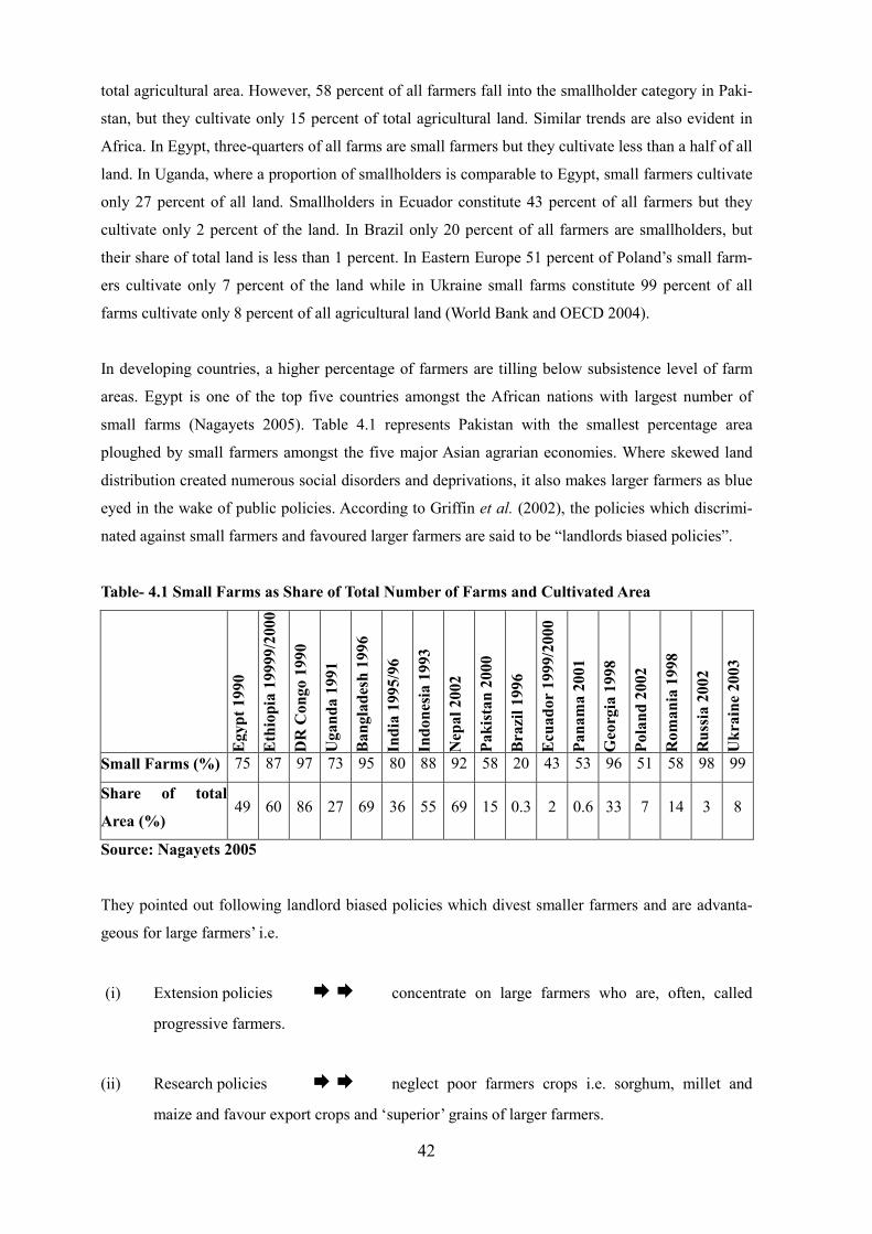
42
total agricultural area. However, 58 percent of all farmers fall into the smallholder category in Paki-
stan, but they cultivate only 15 percent of total agricultural land. Similar trends are also evident in
Africa. In Egypt, three-quarters of all farms are small farmers but they cultivate less than a half of all
land. In Uganda, where a proportion of smallholders is comparable to Egypt, small farmers cultivate
only 27 percent of all land. Smallholders in Ecuador constitute 43 percent of all farmers but they
cultivate only 2 percent of the land. In Brazil only 20 percent of all farmers are smallholders, but
their share of total land is less than 1 percent. In Eastern Europe 51 percent of Poland’s small farm-
ers cultivate only 7 percent of the land while in Ukraine small farms constitute 99 percent of all
farms cultivate only 8 percent of all agricultural land (World Bank and OECD 2004).
In developing countries, a higher percentage of farmers are tilling below subsistence level of farm
areas. Egypt is one of the top five countries amongst the African nations with largest number of
small farms (Nagayets 2005). Table 4.1 represents Pakistan with the smallest percentage area
ploughed by small farmers amongst the five major Asian agrarian economies. Where skewed land
distribution created numerous social disorders and deprivations, it also makes larger farmers as blue
eyed in the wake of public policies. According to Griffin et al. (2002), the policies which discrimi-
nated against small farmers and favoured larger farmers are said to be “landlords biased policies”.
Table- 4.1 Small Farms as Share of Total Number of Farms and Cultivated Area
Egypt 1990
Ethiopia 19999/2000
DR Congo 1990
Uganda 1991
Bangladesh 1996
India 1995/96
Indonesia 1993
Nepal 2002
Pakistan 2000
Brazil 1996
Ecuador 1999/2000
Panama 2001
Georgia 1998
Poland 2002
Romania 1998
Russia 2002
Ukraine 2003
Small Farms (%) 75 87 97 73 95 80 88 92 58 20 43 53 96 51 58 98 99
Share of total
Area (%) 49 60 86 27 69 36 55 69 15 0.3 2 0.6 33 7 14 3 8
Source: Nagayets 2005
They pointed out following landlord biased policies which divest smaller farmers and are advanta-
geous for large farmers’ i.e.
(i) Extension policies � � concentrate on large farmers who are, often, called
progressive farmers.
(ii) Research policies � � neglect poor farmers crops i.e. sorghum, millet and
maize and favour export crops and ‘superior’ grains of larger farmers.
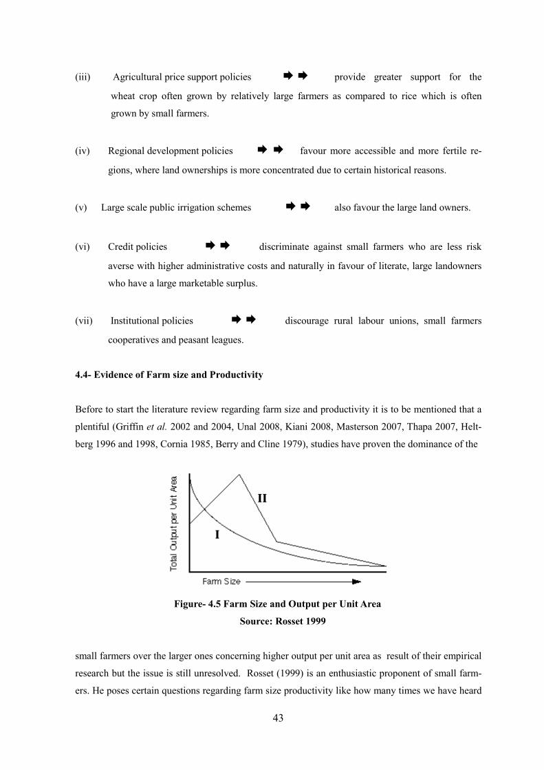
43
(iii) Agricultural price support policies � � provide greater support for the
wheat crop often grown by relatively large farmers as compared to rice which is often
grown by small farmers.
(iv) Regional development policies � � favour more accessible and more fertile re-
gions, where land ownerships is more concentrated due to certain historical reasons.
(v) Large scale public irrigation schemes � � also favour the large land owners.
(vi) Credit policies � � discriminate against small farmers who are less risk
averse with higher administrative costs and naturally in favour of literate, large landowners
who have a large marketable surplus.
(vii) Institutional policies � � discourage rural labour unions, small farmers
cooperatives and peasant leagues.
4.4- Evidence of Farm size and Productivity
Before to start the literature review regarding farm size and productivity it is to be mentioned that a
plentiful (Griffin et al. 2002 and 2004, Unal 2008, Kiani 2008, Masterson 2007, Thapa 2007, Helt-
berg 1996 and 1998, Cornia 1985, Berry and Cline 1979), studies have proven the dominance of the
Figure- 4.5 Farm Size and Output per Unit Area
Source: Rosset 1999
small farmers over the larger ones concerning higher output per unit area as result of their empirical
research but the issue is still unresolved. Rosset (1999) is an enthusiastic proponent of small farm-
ers. He poses certain questions regarding farm size productivity like how many times we have heard
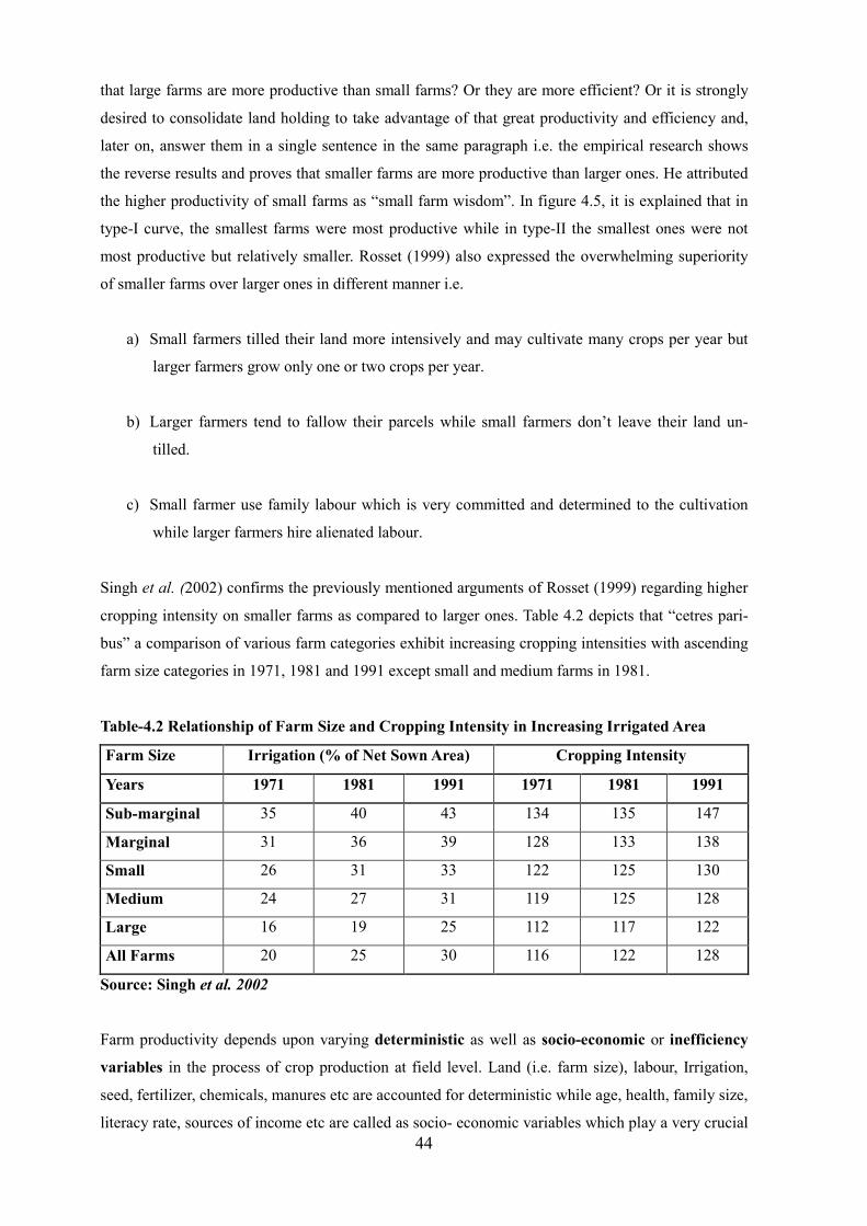
44
that large farms are more productive than small farms? Or they are more efficient? Or it is strongly
desired to consolidate land holding to take advantage of that great productivity and efficiency and,
later on, answer them in a single sentence in the same paragraph i.e. the empirical research shows
the reverse results and proves that smaller farms are more productive than larger ones. He attributed
the higher productivity of small farms as “small farm wisdom”. In figure 4.5, it is explained that in
type-I curve, the smallest farms were most productive while in type-II the smallest ones were not
most productive but relatively smaller. Rosset (1999) also expressed the overwhelming superiority
of smaller farms over larger ones in different manner i.e.
a) Small farmers tilled their land more intensively and may cultivate many crops per year but
larger farmers grow only one or two crops per year.
b) Larger farmers tend to fallow their parcels while small farmers don’t leave their land un-
tilled.
c) Small farmer use family labour which is very committed and determined to the cultivation
while larger farmers hire alienated labour.
Singh et al. (2002) confirms the previously mentioned arguments of Rosset (1999) regarding higher
cropping intensity on smaller farms as compared to larger ones. Table 4.2 depicts that “cetres pari-
bus” a comparison of various farm categories exhibit increasing cropping intensities with ascending
farm size categories in 1971, 1981 and 1991 except small and medium farms in 1981.
Table-4.2 Relationship of Farm Size and Cropping Intensity in Increasing Irrigated Area
Farm Size Irrigation (% of Net Sown Area) Cropping Intensity
Years 1971 1981 1991 1971 1981 1991
Sub-marginal 35 40 43 134 135 147
Marginal 31 36 39 128 133 138
Small 26 31 33 122 125 130
Medium 24 27 31 119 125 128
Large 16 19 25 112 117 122
All Farms 20 25 30 116 122 128
Source: Singh et al. 2002
Farm productivity depends upon varying deterministic as well as socio-economic or inefficiency
variables in the process of crop production at field level. Land (i.e. farm size), labour, Irrigation,
seed, fertilizer, chemicals, manures etc are accounted for deterministic while age, health, family size,
literacy rate, sources of income etc are called as socio- economic variables which play a very crucial
45
role in the process of crop production. Farm size is one of the most important factors of production
and it is also serving as a focal point in this study. The inverse relationship, which means “the
smaller the farm size the greater the output per unit area” has been proven as stylized fact of agricul-
ture in developing countries. The inverse relationship debate was started with the ground breaking
work of Indian author Amartya K. Sen in 1962. Later on, milestone work was done on the issue by
various renowned development economists like Berry and Cline (1979), Bhalla (1979) Cornia
(1985), Carter (1984), Feder (1985), Bhalla and Roy(1988), Benjamin (1995), Masterson (2005 and
2007), Thapa (2007), Unal (2008), etc. Though, the debate regarding farm size productivity depends
upon many factors directly or indirectly but it revolves, mainly, around farm size and labour (i.e.
family, blood sibling, and hired labour) but rest of the factors sink and drown in the seen in various
studies.
To see, whether an inverse relationship amongst factors of production exists, a classical regression
model based on Ordinary Least Square Method (OLS) was,
Classical Regression Model log (y) = α + β log (x) + µ……………………………… (1)
modified by the successors according to the nature and requirements of the research methodologies
with the addition and subtraction of desired and redundant variables, respectively. In the equation (1)
y is the value of monetary or physical output which might be total or output per unit area, x is farm
size including owned, leased in and excluding leased out land and µ is the value of the error term.
The existence of IR can be observed between farm size and productivity with two different methods
of explanations of output and β .e.g. 1) when the value of β is less than unity along with total output,
on the other hand, 2) when its sign is negative exclaiming output per unit area on the left hand side
(i.e. dependent variable) of the equation, respectively.
The studies based on farm size-productivity analysis in which the whole produce is taken as a single
unit but the prices of the various crops grown on the same farm differ significantly across the vari-
ous regions under study, which may cause bias in the final results concerning inverse relationship
research (Bardhan 2003). The forthcoming section of the chapter would unveil the facts regarding
four major factors affecting inverse relationship of farm productivity which delineates deterministic
as well as socio-economic phenomenon of agriculture production. The key controversy in the IR
studies like i) mis-specification or mis-identification hypothesis was emphasized and proved by
Bhalla and Roy (1988), ii) labour duality or bimodal or agricultural dualism iii) factor market imper-
fections and iv) farmer’s attributes displayed causal effects to give policy implications in the end of
IR studies in the form of land redistribution. Nevertheless, the turning down of IR phenomenon
cause to advocate large farms in the end of these studies. The up coming parts would explain how
aforementioned four major factors affect inverse relationship in the light of previous literature.
46
4.4.1 Mis-Specification in Farm Productivity Analysis
The mis-specification issue was arose as a heart of inverse yield relationship debate exhibiting the
fact, small farmers own more fertile lands as compared to larger farmers and it was put forth that
inter-village IR is more robust as compared to intra-village (Cornia 1985, Benjamin 1995 and Sen
1999). Furthermore, fertile lands support dense populations resulting in higher fragmentations,
whereas at the time of financial bottlenecks low quality lands is sold first and consequently smaller
farmers are more likely to have higher quality lands. It is crucial to account for land quality to ob-
serve the systematic inverse yield relationship (Unal 2008). Heltberg (1998) defined impact of land
quality on the farm productivity phenomenon by elaborating it in a way that if land quality is in-
versely proportional to the size of farm then its omission from the regression modeling would show
the spurious results. In addition, he said that the value or sign of beta would confirm inverse rela-
tionship. A systematic relationship between land quality and farm size is possible (Sen 1966, 1975),
and to avoid from unbiased results it would be, very, vital to account for land quality. The “stylized
fact” of inverse relationship was challenged by Bhallah and Roy (1988) for the first time on the ba-
sis of this hypothesis after almost two and half decades of its inception and its proven existences in
several studies including famous Cornia (1985), and Berry and Cline contributions (1979). He
worked on Indian macro level data and found presence of inverse relationship in 16 Indian States out
of 17. But the conformity of the results was severely damaged, when he run regression on disaggre-
gated data at district level and found that IR existed only in 51 districts out of 176. The authors con-
cluded that unobserved land fertility can, better, be accounted for, by disaggregating geographical
units and they also concluded, disaggregated data would distort or reverse the importance of IR. But
later on, the conclusions were rejected by Heltberg (1998) and Unal (2008) on the basis of following
methodological flaws in the study,
A) The sample size was much smaller as a result of disaggregation which would have entailed a
large loss of degree of freedom.
B) District level disaggregation avoid heterogeneity within districts while it only accounted for
inter district heterogeneity.
In Pakistani Punjab, village level study by Berry and Cline (1979), based on much more homogene-
ous but disaggregated sample than Bhalla and Roy found strong existence of IR.
47
4.4.2 Labour Duality: Mode of Production
Labour duality (Kiani 2008), agriculture dualism (Sen 1966), mode of production (Chayanov 1966,
Unal 2008) or “bimodal agriculture production” (Cornia 1985) are similar terms used in various
studies to explain the relationship between labour and land and their impact on farm productivity.
It is a well accepted fact that Sen’s (1962, 1966) theory of agricultural dualism was the first ac-
count of size-output relationship which flared up the debate of inverse relationship. He described in
his theory that peasantry is severely credit constrained but endowed with plenty of family labour
with zero or minimum opportunity cost. On the other hand, larger farmers have better access to
credit but they have to rely on expensive hired labor. Nevertheless, small farmers apply more labour
per unit area as compared to capitalists. He added that this kind of functioning reduces productivity
and augments profitability per unit area with increasing farm size when cost of family labour is
based on imputed market wages.
Cornia (1985) claimed that agricultural production is carried out under bimodal conditions; larger
farms cultivate their lands by keeping fallow a big portion of it but small farmers undergo inverse
conditions with excess labour with little opportunity of productive work on their farms. It is obvious
that small farmers are different from larger ones in many ways; they cultivate a larger portion of
their land, intensive use of labour is used in each crop activity, land terracing, canalization and land
infrastructure is managed in a better way by the small farmers which require more intensive use of
labour.
Lamb (2003) argues that according to the classical model of labour market dualism, small farmers
are unable to market their labour and they over allocate it to their own farms. Consequently, the
marginal productivity of their labour is lower than the market wage rate. Carter (1984) re-affirms by
contradicting a bit from the previous statement quoting that the cause of inverse relationship is over-
allocation of family labour as well as other variables but family labour alone does not suffice to cre-
ate inverse relationship alone.
It is suggested that dual labour markets contribute, primarily, to the existence of inverse relation-
ship. Dual labour markets mean that plenty of labour is involved in small farm production and the
labour to land ratio is much higher than on larger farms. Masterson (2007) said, the cheaper family
labour is a basic reason for higher labour to land ratios on the small farms. It is quite apparent that
due to sincere and higher efforts of family labour than hired labour make their opportunity cost
lower (Mazumdar 1965). Sen (1975) argued that workers prefer to work either for themselves or for
their family rather to work for some one else. The family workers can produce more can be ex-
plained on the basis of three proposition put forth by Feder (1985), a) family labour is more efficient
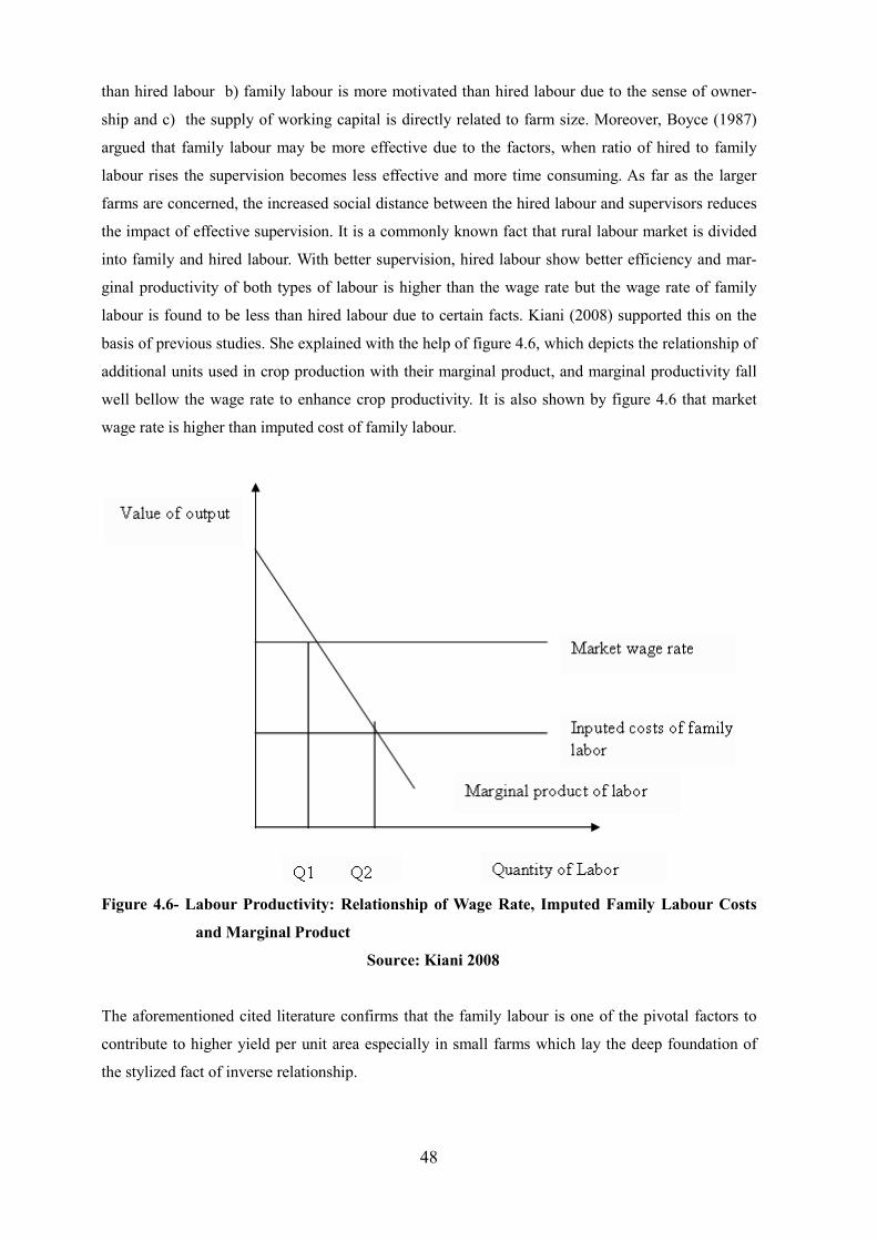
48
than hired labour b) family labour is more motivated than hired labour due to the sense of owner-
ship and c) the supply of working capital is directly related to farm size. Moreover, Boyce (1987)
argued that family labour may be more effective due to the factors, when ratio of hired to family
labour rises the supervision becomes less effective and more time consuming. As far as the larger
farms are concerned, the increased social distance between the hired labour and supervisors reduces
the impact of effective supervision. It is a commonly known fact that rural labour market is divided
into family and hired labour. With better supervision, hired labour show better efficiency and mar-
ginal productivity of both types of labour is higher than the wage rate but the wage rate of family
labour is found to be less than hired labour due to certain facts. Kiani (2008) supported this on the
basis of previous studies. She explained with the help of figure 4.6, which depicts the relationship of
additional units used in crop production with their marginal product, and marginal productivity fall
well bellow the wage rate to enhance crop productivity. It is also shown by figure 4.6 that market
wage rate is higher than imputed cost of family labour.
Figure 4.6- Labour Productivity: Relationship of Wage Rate, Imputed Family Labour Costs
and Marginal Product
Source: Kiani 2008
The aforementioned cited literature confirms that the family labour is one of the pivotal factors to
contribute to higher yield per unit area especially in small farms which lay the deep foundation of
the stylized fact of inverse relationship.
49
4.4.3 Factor Market Imperfections
The mal-functioning of agricultural factors markets due to some particular reasons are designated as
rural market imperfections. The central theme of this hypothesis in the inverse relationship debate is
that different prices of various inputs are the fundamental reason to use varying amounts of inputs on
their farms. (Mazumdar 1965, Sen 1966, Berry and Cline 1979, Sen 1981, Cornia 1985, Eswaran and
Kotwal 1986, Griffin et al. 2002, Benjamin and Brandt 2002,)
In a neoclassical world, in a perfect market scenario with same prices of factors of production it is
forecast that all factors of production can be fully utilized, and resources are allocated efficiently across
alternatives uses. Hence, no systematic yield difference will be observed (Schultz 1964, Heltberg
1998). Unal (2008) corroborated perfect market idea by ascribing it to two major factors of production
i.e. land and labour, and she assumed constant return to scale operating under the same production
function. She added that in a perfect market mechanism when the land is more productive than labour it
should be transferred to small farms while more productive labour should be shifted towards larger
farms. As a result, small and large farms should undergo similar marginal rates of technical substitu-
tion. In this way, agricultural production would be attained free of inverse relationship. In the end, the
puzzle was solved by commenting that factor markets are imperfect and so the resource allocation is
inefficient across the agricultural production process.
Cornia (1985) in a study of 15 developing countries observed IR phenomenon by using different factors
as independent variables like land use intensity, share of cultivated land, labour in man days while
irrigation, fertilizer, pesticides and fuel etc were utilized as intermediate inputs. He found that Bangla-
desh, Peru and Thailand, which were more densely populated and with very small holdings deviated
from inverse relationship, while the rest 12 countries showed stronger inverse relationship results. He
concluded from the result of the study, inverse relationship prevails due to better management of
intermediate as well as primary inputs i.e. land and labour on the small farms. Moreover, small and
larger farmers are exposed to different prices regarding labour and capital i.e. prices of labour are
higher for large farms while capital is more expensive for small farms.
Land and labour are the two fundamental factors of production in the agricultural sector. Due to the
profound importance of labour it was decided to accommodate it in a small but separate section.
Although, land is equally important, not only, in the agricultural sector and especially in the inverse
relationship studies but to avoid from unnecessary protraction, it has been decided to incorporate it with
some other factors. Land market imperfections are one of the fundamental causes of inverse relation-
ship phenomenon and it affects per unit farm productivity in two ways i.e. through imperfect land rental
markets and imperfect land sale markets (Heltberg 1998). As a result of “Marshallian inefficiency law”
many developing countries followed the vague land tenurial reforms (Skaufias 1995), especially in
50
South Asia as a so called land to the tillers adherents which seriously curtailed land rental markets
especially for long term lease (Hayami and Otsuka 1993, Shaban 1987). In the two major form of land
rents i.e. share cropping and fixed rent to some certain ex-ante and ex-poste conditions prevent lan-
downers to follow suite as it is required. Share cropping is curtailed due to the fact that tiller does not
employ optimal use of inputs and, consequently, attain lower yields per unit area and owners have to
face loss in this respect. As far as the fixed rent is concerned, the owners should be contented in this
kind of lease but tenants have to bear whole responsibility. As a matter of fact, If the rent is to be paid
in advance, the credit constrained farmers might hesitate to lease in land as described by Feder (1985),
and Eswaran and Kotwal (1986). While in case of after payment, owners are skeptical or uncertain
whether the tenants would pay the agreed amount or not? (Wiens 1977).
According to Heltberg (1998), the major reason for imperfect land sale markets is the failure of farmers
to adjust their holdings according to the size of their family workers. This trend can be explained in
following manner,
a) Government interventions whether they are, in form of inputs or outputs, are not neutral to scale.
These interventions are always in favour of landed elites to intact their economic and political power as
a result of successful lobbying by feudals (Griffin et al. 2002, Carter and Barham 1996, Binswanger et
al. 1995).
b) In some parts of the world, land markets might be thin and restricted to sell land to the outsider.
c) Small farmers are usually unable to mobilize their resources for credit and savings to finance land
purchases and heavy transaction costs do not allow them to follow suit. But, some times small farmer
sell their land for their subsistence which is an opportunity for larger holders to concentrate more
(Carter and Wiebe 1990).
d) Land is an asset of insurance, power, prestige and bondage. It also a place of ancestral home, and it is
a portfolio asset to hedge against inflation in countries with underdeveloped capital markets and it
serves as collateral for credit (Cornia 1985, Kaldjian 2001, Platteau 1992).
Hence, imperfect land markets significantly hamper the farm efficiency due to the distorted equation of
family workers endowments’ and farm size. Secondly, land accumulation due to imperfect land markets
cause supervision constraints on the hired labour at bigger farms which is a basic reason of inverse
relationship in farm production (Heltberg 1998).
As far as the capital markets imperfections are concerned, there are very strong pros and cons of it
regarding inverse relationship theory in the agricultural sector. Ceteris paribus, imperfect credit markets
51
make it difficult for the bigger landlords to plough it efficiently because they cannot, readily, borrow
money from the market when they direly need it and inverse relationship might be a reason of this fact.
Contrarily, farmers can access credit, conditionally, by pledging their lands as collaterals (Binswanger
and Rosenweig 1986) and financial institutions may also charge some fix fee or may have some certain
“minimum standard amount of loan” which can work as restraint for the small farmers to obtain credit
from the formal institutions. But larger farmers can work efficiently and enhance their output benefiting
from collateral conditions by attaining credit (Feder 1985, Feder and Onchon 1988), this fact exposes
the weakening of inverse relationship. However, when operative land holding plead for supervision
constraint of the larger holdings affecting inverse relationship, at the same time ownership holding
caters evidence concerning credit constraint (Heltberg 1998). Cornia (1985) argues that financial
institutions are not well developed in rural areas as a result of which farmers have to rely on local
informal money lenders with higher, usurious, interest rates. He added that credit available on soft
terms basis goes to the richer peasants due to their better reputation regarding returning capacity plus
they use their influence to channelize official finance to the rural areas. In the end he noted that cost and
access to credit may be inversely proportional to the farm size.
The debate concerning imperfect credit markets is quite ambiguous with its positive or negative
relevance to the inverse relationship. As far as collateral conditions for credit availability is concerned,
it seems more rational that easy access and availability of credit to the larger farmers might weaken
the inverse relationship in the agriculture by making bigger estates more productive than smaller ones
but latest studies reiterate that inverse relationship strongly exist at its full fledge scale (Unal 2008,
Kiani 2008, Thapa 2007, Matchaya 2007, Fan and kang 2005).
4.4.4 Farmers Attributes: Family Size, Age and Education
Farmer’s heterogeneity can be explained in terms of certain characteristics of households and house-
hold heads. In the farm size-output relationship, the literature, mainly, includes size of the household as
well as age and education of household head. Logically speaking, mounting family size and increasing
education of household head should influence positively while rise in age of household head should
reduce yield per acre, as age affect decision making capability and repel the adoption process of new
technology. Through a keen and detailed survey of literature it has been found that there are few output-
farm size relationship studies which incorporate socio-economic or demographic variables. On the
other hand, the literature regarding farm efficiency either on the basis of single crop or studying whole
farm integrated demographic variables in econometric models to observe their impacts.
Miller (2008) explained the positive and negative signs of linear as well as quadratic terms to divulge
relationship of age of household head and labour productivity at the farm level. He found the mean age
of operator 55.39 years and he concluded that when this value is increased by one standard deviation
52
labour productivity decreases by 6.71 percent. Furthermore, he observed the rise in farm productivity
with the decrease in average ages of the respondent. Similarly, Villatoro (2007) studied the relationship
between farm growth rate (i.e. nominal assets, real assets including farm area, and number of workers)
and operator age. He concluded that increasing age of household head obstructs or negatively affects
the growth rate of assets.
In a farm size-yield relationship study, Matchaya (2007) concluded that age of the household head in 5
districts of Malawi was found to be negatively related to farm productivity while level of education (i.e.
years of schooling as a proxy for farmers ability) was found to be positive.
In the beginning of the green revolution Schultz (1964) put forth his opinion regarding education and
farm productivity relationship by arguing that education can increase productivity and Sen (1999)
favoured his view and said, literate farmers can read the instructions on the machines and have better
capability to apply new techniques to enhance productivity. Unal (2008) did not turn down aforemen-
tioned statements but she added that, though, small farmers lack access to such machines but they are
still more productive than larger farmers.
Asadullah and Rehman (2006) studied 141 villages for farm productivity and efficiency with a special
focus on education along with other variables in Bangladesh. But they concluded that impact of land
dominated all other factors of production e.g. one percent increase in land enhances 0.65-0.71 percent
rice production. In addition, increase in one year of schooling of household head or any adult family
member affects positively the rice production i.e. 3-6 percent. They observed that by controlling
education of households head or adult family members in a regression model, make the results insigni-
ficant.
As far as the effect of family size on productivity is concerned Chayanov (1926) was the first to draft a
book on the issue of peasant and their demographic behavior on farm productivity. He argued that the
basic objective of a peasant worker is subsistence and he strives, accordingly, keeping in mind family
needs. Chayanov added that greater the family members mean higher yield to be produced and vice
versa. Thapa (2007) is one of the agriculture economists who focused special attention on farm produc-
tivity and family size relationship in his work. He concluded that, although, family size plays a crucial
role in the crop production process but in case of larger farms its share is not much stronger with the
better access to resources e.g. credit, advanced technology, irrigation and market information. Further-
more, bigger family size is pivotal for family farms because it is highly conducive to work efficiently,
conditional, with better access to resources. In addition, family size and other socio-economic characte-
ristics do help in production decisions in rural economies which, ultimately, affect farm productivity.

53
The conclusion on the basis of facts presented in the chapter would reveal that there must be an evolu-
tion of some mechanism to reduce inequality in asset holdings which will definitely diminish food
insecurity threats. It would also alleviate poverty and would help to boost up development process in
the developing countries. However, it is strongly needed to restructure the farm size to produce and
employ labour intensive technologies to decrease rural unemployment. It will also help to attain food
security and alleviate poverty of 80 percent poor of the world living in rural areas.
54
CHAPTER-5
DATA SOURCES AND ANALYTICAL TOOLS
This undergoing study has been devised to observe, mainly, land distribution disparities and produc-
tivity differentials in three different areas based on irrigation endowments and various farm sizes.
Various approaches were employed in order to examine the land distribution, tenancy structure,
cropping pattern, cropping intensity and crop diversity of the farmers by disintegrating total numbers
of farming households in three distinct size groups. Furthermore, inverse relationship between yield
per hectare and factors of production with special emphasis on operational land holding in the study
area was also examined by taking up econometric model. The chapter has been organized in to two
major portions following their sub-parts to express data types and sampling methods, data collection,
analytical tools and techniques to achieve set objectives of the study.
5.1- Data Sources
5.1.1- Types
Two types of data sources were used i.e. primary as well as secondary data. A huge amount of pri-
mary data comprising of many thousand variables was collected from the field as part of project
launched in district Gujrat and Mandi Bahauddin titled as “Impact Assessment of Irrigation Infra-
structure Development on Poverty Alleviation” by the International Water Management Institute
(IWMI) Lahore, Pakistan. The data with some relevant selected variables was, later on, attained from
IWMI with kind support of Dr Intizar Hussain (Executive Director of International Network for Par-
ticipatory Irrigation Management) for the purpose of this study. The further details about data are
being laid out in a forthcoming section of the chapter. As far as the secondary data is concerned, the
office of Agriculture Census Organization, Punjab Economic Research Institute (PERI), Interna-
tional Network for Participatory Irrigation Management and University of Agriculture Faisalabad
were visited in search of some relevant reliable secondary data. Afterwards, on the basis of consulta-
tions and discussions with professionals of the aforementioned organizations the data was extracted
from various sources like Agriculture Census Reports of Pakistan 1960, 1972, 1980, 1990 and 2000,
Agriculture Census Reports of Punjab 2000, Punjab Development Statistics 2008, various reports of
Food and Agriculture Organization, different World Bank publications. Some publications of Punjab
Economic Research Institute were also thrashed to obtain concerned secondary data as a supplement
to highlight and emphasize the scope of the study.
55
5.1.2- Site Selection and Sampling Methods
To start with, a general survey of the site, was done by the project team to get knowledge of the area
regarding local agricultural methods, climate and cropping patterns. Above all, the purpose was to
identify specific sites for the project. These visits gave a good insight of the area concerning living
standard, overall sources of income, dependence on agriculture etc inside the villages of district Gu-
jrat and Mandi Bahauddin. Tehsil Kharian of district Gujrat was abandoned as study area in the pro-
ject due to a large number of its inhabitants being employed abroad in the Middle East and Europe.
Four different sites were selected with different patterns of irrigation endowments, two amongst
them were “irrigated perennial areas” (i.e. with year round canal irrigation) with a minor difference
of crop rotation, a third one was “irrigated non-perennial area” (i.e. with 6 months canal irrigation).
While the fourth area opted for the project was without any public canal irrigation infrastructure. It
was observed that most of the farmers rear their crops through own tubewell irrigation or by purchas-
ing water from the neigbours but this area has been considered as “rainfed” due to the lack of public
irrigation facilities. The purpose of this study is entirely different from the mother project, so the
selected areas have been modified according to the scope and requisites of this study. It is worth-
mentioning here, both perennial areas were dealt as a single entity by adding them together and titled
“irrigation perennial area” in the study while the rest two areas were kept same as “irrigated non-
perennial area” and “rainfed area”. Figure 5.1 shows irrigated and rainfed territories in district Gujrat
and Mandi Bahauddin.
To avoid any kind of bias in the final results, stratified random and cluster sampling methods were
adopted to select the households for the purpose of primary data collection in the study area. Irri-
gated areas were selected along the Upper Jehlum and Gujrat Branch canals. The canals as well as
watercourses were divided into three distinct areas by taking special care to avoid mixing up the
boundaries of adjacent water channels. A strong vigilance was kept that each respondent be from its
own cluster i.e. head, middle and tail. The data was collected along the water source i.e. from head,
middle and tail following the typical style of International Water Management Institute because it
yields, definitely, better results which help to give bias free policy implications at the end of the
study. The mother project was to observe the poverty differentials on head, middle and tail of the
irrigation source and sampling and data collection was done accordingly but to describe all those
methods is beyond the scope of this study. So, it is favourable, just, to mention the tools concerning
this ongoing study.
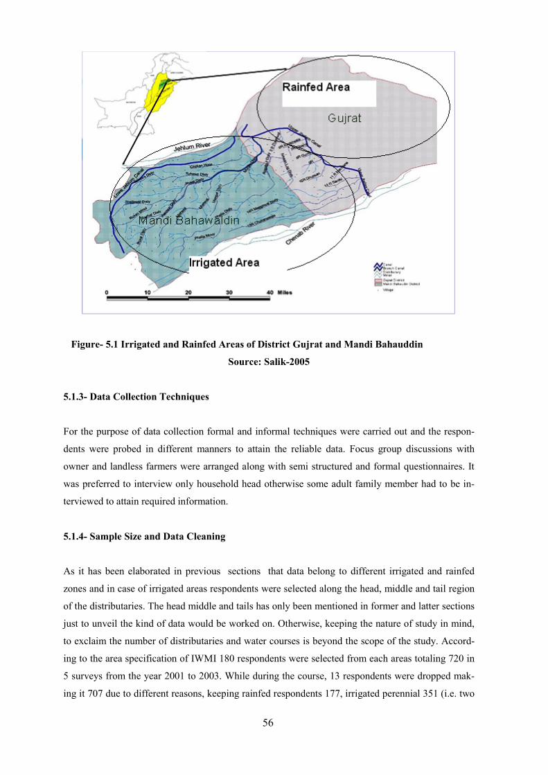
56
Figure- 5.1 Irrigated and Rainfed Areas of District Gujrat and Mandi Bahauddin
Source: Salik-2005
5.1.3- Data Collection Techniques
For the purpose of data collection formal and informal techniques were carried out and the respon-
dents were probed in different manners to attain the reliable data. Focus group discussions with
owner and landless farmers were arranged along with semi structured and formal questionnaires. It
was preferred to interview only household head otherwise some adult family member had to be in-
terviewed to attain required information.
5.1.4- Sample Size and Data Cleaning
As it has been elaborated in previous sections that data belong to different irrigated and rainfed
zones and in case of irrigated areas respondents were selected along the head, middle and tail region
of the distributaries. The head middle and tails has only been mentioned in former and latter sections
just to unveil the kind of data would be worked on. Otherwise, keeping the nature of study in mind,
to exclaim the number of distributaries and water courses is beyond the scope of the study. Accord-
ing to the area specification of IWMI 180 respondents were selected from each areas totaling 720 in
5 surveys from the year 2001 to 2003. While during the course, 13 respondents were dropped mak-
ing it 707 due to different reasons, keeping rainfed respondents 177, irrigated perennial 351 (i.e. two
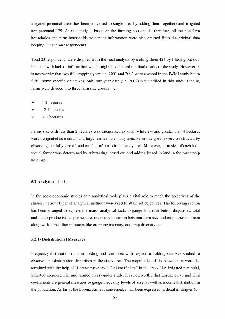
57
irrigated perennial areas has been converted to single area by adding them together) and irrigated
non-perennial 179. As this study is based on the farming households, therefore, all the non-farm
households and farm households with poor information were also omitted from the original data
keeping in hand 447 respondents.
Total 23 respondents were dropped from the final analysis by making them 424 by filtering out out-
liers and with lack of information which might have biased the final results of the study. However, it
is noteworthy that two full cropping years i.e. 2001 and 2002 were covered in the IWMI study but to
fulfill some specific objectives, only one year data (i.e. 2002) was untilled in this study. Finally,
farms were divided into three farm size groups’ i.e.
� < 2 hectares
� 2-4 hectares
� > 4 hectares
Farms size with less than 2 hectares was categorized as small while 2-4 and greater than 4 hectares
were designated as medium and large farms in the study area. Farm size groups were constructed by
observing carefully size of total number of farms in the study area. Moreover, farm size of each indi-
vidual farmer was determined by subtracting leased out and adding leased in land in the ownership
holdings.
5.2 Analytical Tools
In the socio-economic studies data analytical tools plays a vital role to reach the objectives of the
studies. Various types of analytical methods were used to attain set objectives. The following section
has been arranged to express the major analytical tools to gauge land distribution disparities, total
and factor productivities per hectare, inverse relationship between farm size and output per unit area
along with some other measures like cropping intensity, and crop diversity etc.
5.2.1- Distributional Measures
Frequency distribution of farm holding and farm area with respect to holding size was studied to
observe land distribution disparities in the study area. The magnitudes of the skewedness were de-
termined with the help of “Lorenz curve and “Gini coefficient” in the areas (.i.e. irrigated perennial,
irrigated non-perennial and rainfed areas) under study. It is noteworthy that Lorenz curve and Gini
coefficients are general measures to gauge inequality levels of asset as well as income distribution in
the population. As far as the Lorenz curve is concerned, it has been expressed in detail in chapter 6.
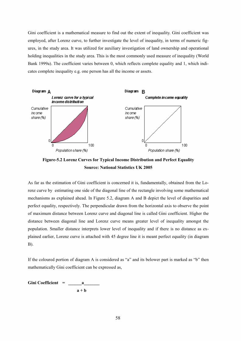
58
Gini coefficient is a mathematical measure to find out the extent of inequality. Gini coefficient was
employed, after Lorenz curve, to further investigate the level of inequality, in terms of numeric fig-
ures, in the study area. It was utilized for auxiliary investigation of land ownership and operational
holding inequalities in the study area. This is the most commonly used measure of inequality (World
Bank 1999a). The coefficient varies between 0, which reflects complete equality and 1, which indi-
cates complete inequality e.g. one person has all the income or assets.
Figure-5.2 Lorenz Curves for Typical Income Distribution and Perfect Equality
Source: National Statistics UK 2005
As far as the estimation of Gini coefficient is concerned it is, fundamentally, obtained from the Lo-
renz curve by estimating one side of the diagonal line of the rectangle involving some mathematical
mechanisms as explained ahead. In Figure 5.2, diagram A and B depict the level of disparities and
perfect equality, respectively. The perpendicular drawn from the horizontal axis to observe the point
of maximum distance between Lorenz curve and diagonal line is called Gini coefficient. Higher the
distance between diagonal line and Lorenz curve means greater level of inequality amongst the
population. Smaller distance interprets lower level of inequality and if there is no distance as ex-
plained earlier, Lorenz curve is attached with 45 degree line it is meant perfect equality (in diagram
B).
If the coloured portion of diagram A is considered as “a” and its belower part is marked as “b” then
mathematically Gini coefficient can be expressed as,
Gini Coefficient = ______a_______
a + b
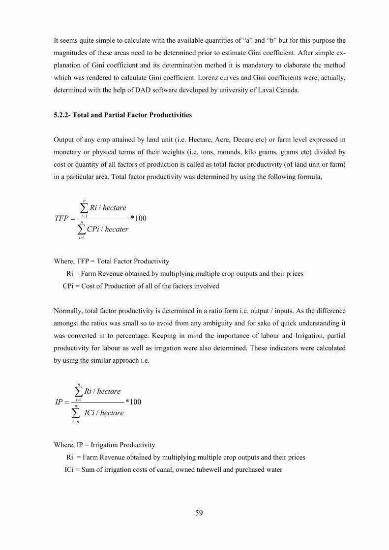
59
It seems quite simple to calculate with the available quantities of “a” and “b” but for this purpose the
magnitudes of these areas need to be determined prior to estimate Gini coefficient. After simple ex-
planation of Gini coefficient and its determination method it is mandatory to elaborate the method
which was rendered to calculate Gini coefficient. Lorenz curves and Gini coefficients were, actually,
determined with the help of DAD software developed by university of Laval Canada.
5.2.2- Total and Partial Factor Productivities
Output of any crop attained by land unit (i.e. Hectare, Acre, Decare etc) or farm level expressed in
monetary or physical terms of their weights (i.e. tons, mounds, kilo grams, grams etc) divided by
cost or quantity of all factors of production is called as total factor productivity (of land unit or farm)
in a particular area. Total factor productivity was determined by using the following formula,
1
1
/
*100
/
n
i
n
i
Ri hectare
TFP
CPi hecater
=
=
=∑
∑
Where, TFP = Total Factor Productivity
Ri = Farm Revenue obtained by multiplying multiple crop outputs and their prices
CPi = Cost of Production of all of the factors involved
Normally, total factor productivity is determined in a ratio form i.e. output / inputs. As the difference
amongst the ratios was small so to avoid from any ambiguity and for sake of quick understanding it
was converted in to percentage. Keeping in mind the importance of labour and Irrigation, partial
productivity for labour as well as irrigation were also determined. These indicators were calculated
by using the similar approach i.e.
1
/
*100
/
n
i
n
i n
Ri hectare
IP
ICi hectare
=
=
=∑
∑
Where, IP = Irrigation Productivity
Ri = Farm Revenue obtained by multiplying multiple crop outputs and their prices
ICi = Sum of irrigation costs of canal, owned tubewell and purchased water
60
To determine labour productivity family labour man days were converted in to monetary terms by
multiplying it with predetermined average per day wage (i.e. 100 Rupees) of the study area. Fur-
thermore, hired labour and family labour man days in monetary form were added together to attain
labour productivity of the study area.
1
1
/
*100
/
n
i
n
i
Ri hectare
LP
LCi hectare
=
=
=∑
∑
Where, LP = Labour Productivity
Ri = Farm Revenue obtained by multiplying multiple crop outputs and their prices
LCi = Family and hired labour costs together incurred on crop production
5.2.3- Crop Diversity
Crop diversity is derived from biodiversity concepts but in agricultural production research it can be
associated with extension of cropping pattern. On the other way, it can also be explained as number
of various kinds of crops grown in the study area based on their species and cultivars etc. Inverse of
Herfindahl Index was utilized to determine crop diversity index in the study area. Crop diversity
index was determined by using following mathematical equations i.e.
CDI 2
1
1n
i
i
S=
=
∑
Where, CDI = Crop Diversity Index
Si is share of individual crops in total cropped area
This measure was simply used to quantify the diversification level of farmers on the basis of crops in
the study area.
5.2.4- Cropping Intensity
Cropping Intensity is defined as “total cropped area or total sown area in terms of total cultivated
area multiplied by 100 or it indicates the extent to which the cultivated area was used for cropping.
This is an extremely good measure to determine the intensiveness of agriculture per annum in form
of crop production in a specified area. Following formula were utilized to determine cropping Inten-
sity in the various study locations as well as at different farm size categories,
61
1 *100
n
i
TCAi
CICA
==∑
Where, CI= Cropping Intensity
TCAi = Total cropped area and CA = Cultivated area
5.2.5- Kruskal Wallis Test: A Test for Research Hypothesis Verification
Kruskal Wallis test was utilized to test the hypothesis of the study. This is most commonly used
measure when data does not fulfill normality assumptions for analysis of variance (ANOVA) and
homogeneity of variance of the means of samples. Keeping in mind the pre- requisites of Kruskal
Wallis test data was tested for normality and homogeneity of variance by using Kolmogorov-
Smirnov as well Levene’s test, respectively. The results of normality and homogeneity of variance
fulfilled the pre-requisites of the Kruskal Wallis while deviated from ANOVA. Statistical Package
for Social Sciences (SPSS) was used to render Kruskal Wallis measure to test the hypothesis. It will
be worth mentioning here to describe the method that how Kruskal Wallis test works to test the hy-
pothesis? To observe the difference amongst various farm size productivities following null and
alternative hypothesis were used to test i.e.
Null hypothesis Ho = There is no significant difference amongst the mean productivities of small,
medium and large farms of study area.
Alternative hypothesis H1 = There is a significant difference in the mean productivities of small,
medium and large farms of study area.
Similar procedure was adopted to test all of the rest hypothesis i.e. partial productivities, gross mar-
gins, on and off farm incomes etc at maximum probability level of 10 percent. The significance level
of the results to show probability level in each table has been marked with number of stars. Results
with *, ** and *** show significance at 1, 5 and 10 percent probability levels.
5.2.6- Econometric Model
Econometric tools were employed to observe existence of kind of relationship amongst various vari-
ables utilized in the study. Output per hectare was used as dependent variable to observe the impact
of various regressors upon it. “Log-log function” was used by employing Ordinary Least Square
(OLS) method to investigate the relationships of the variables on both sides of the equation whether
62
it was positive or negative. A description of dependent and independent variables used in economet-
ric models has been presented as under,
A) Dependent variable
Abbreviations Names of Variables
• yield = yield / hectare
B) Independent variables
• Opholding = farm Size
• Irrigation = irrigation Cost / hectare
• Labour =labour man days/ hectare (family labour +hired labour)
• Int.inputs = Intermediate input costs ( i.e. seed + fertilizer + manure + chemi
cal + mechanization) / hectare
• F.size = Family size
• Credit = Credit / hectare
• Agehead = Age of household head
• eduhead = Education of household head
• %FW = Percentage of family workers working in agriculture sector
• NF income = Non-farm income of households
• Downtractor =Dummy variable of own tractor
• Downtubewells = Dummy variable of own Tubewell
Natural logs of all of the variables were taken before to start analysis. To avoid multicollinearity
problems and to reduce the number of variables different kinds of input cost were added together
under the name of “int.inputs”. The modeling was done in SPSS to achieve better and reliable results
of the study. The following model was used to see relation between dependent variables and the
independent variables for all study locations.
C) Model- to observe existence of Inverse Relation between output and factors of production
∑ ∑ ∑ ∑ ∑ ∑ ++++++= creditIninputsInirrigationInlabourInOpholdingInYieldIn 54321 .int βββββα
∑ ∑ ∑ ∑∑ +++++ SizeFInNFIncomeInFWInllDowntubeweInrDowntractoIn .% 109876 βββββ
11 12In agehead In educationhead eβ β+ +∑ ∑
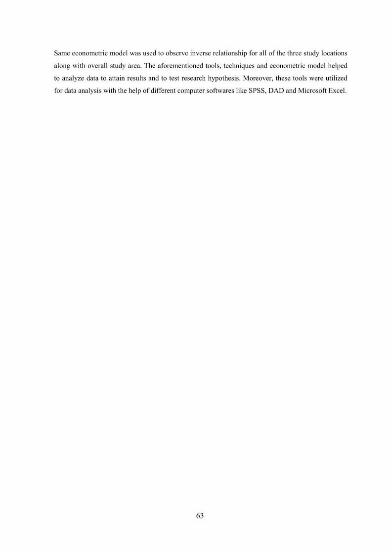
63
Same econometric model was used to observe inverse relationship for all of the three study locations
along with overall study area. The aforementioned tools, techniques and econometric model helped
to analyze data to attain results and to test research hypothesis. Moreover, these tools were utilized
for data analysis with the help of different computer softwares like SPSS, DAD and Microsoft Excel.
64
CHAPTER- 6
LAND DISTRIBUTION AND PRODUCTIVITY ANALYSIS
A VIEW OF INVERSE RELATIONSHIP
The detailed description of the study areas was elaborated regarding farm and family characteristics,
land tenure structure and cropping patterns of the farmers of the various farming systems in chapter-
3. This present chapter has been drafted to articulate the observed land distribution disparities, crop-
ping intensity and diversity, farm productivities, and the existence or absence of inverse relation-
ships between farm size and productivity along with some other indicators. All of the indicators have
been quantified on the basis of various study locations and comparison amongst different farm size
categories. The outcome of data analysis is expressed in tabular as well as in graphical format to
better understand the spirit of the results. This chapter can be recognized into three distinguished
portions: the first portion is started with description of “land distribution disparities” in form of
quintiles representing the numbers of households followed by Lorenz curve and Gini coefficient in
the study area. Subsequently, cropping intensity, crop diversity, farm productivity comprising of
total and partial factor productivities and gross margins also share this portion of the chapter. While
next portion of the chapter consists of wealth distribution corroborated on the basis of land distribu-
tion disparities following share of farm and off farm income of the farmers and institutional credit
availability in the study area. While last segment of the chapter divulges the results of the regression
model used for the sake of inverse relationship exploration in the study area. This section expresses
the relationship of the yield trends per hectare with farm size and other factors of production which
was the second major motive following land distribution disparities to undertake this study. The
validity of “stylized fact” of inverse relationship examined in this portion of the chapter would guide
towards major policy recommendations at the end of the thesis write up. Hypothesis needs to be
restated to observe compliance or defiance of the results from them in the following sections.
6.1- Hypothesis Restated
1. Land distribution is skewed in overall study area as well as in the various farming systems i.e.
irrigated perennial, irrigated non-perennial and rainfed areas
2. Cropping intensity, crop diversity, total and partial factor productivities (i.e. irrigation and la-
bour productivities), gross margins, income distribution etc are higher in evenly land distri-
buted study location as compared to others.
65
3. All of the aforementioned indicators except labour productivity yield better results at small
farms as compared to other farm size categories in each study location as well as overall
study area.
4. Inverse relationship of farm size and productivity is a valid proposition and it exists in each
study location i.e. irrigated perennial, irrigated non-perennial and rainfed areas under study.
6.2- Extent of Land Inequality in the Study Area
This section of the chapter, being the foremost significant component of the study, expresses results
concerning degree of inequality and land distribution skewedness in the various areas under study.
Various measures have been carried out to gauge land distribution disparities in the area. An attempt
has been made to delineate relationship between number of holdings and farm area. It starts with
simple graphical representation of owned and operational land holdings, explaining percentage of
owned with percentage of operational farm area distribution in different quintiles in ascending order.
Afterwards, Lorenz curve and Gini coefficient present a more comprehensible view regarding land
inequality in the area. This section would conclude the outcomes showing their relevance or contra-
dictions to the concerned research hypothesis at the end.
6.2.1- Percentage Distribution of Owned and Operational Farm Area
Figure-6.1 expresses the percentage of owned and operational farm area under cultivation in five
equal partitions of total number of households in the form of quintiles. Each quintile represents 20
percent farmers in ascending order from lowest 20 percent to highest category. It can, easily, be
grasped that percentage ownership and operational holding area rise with every subsequent quintile
and it can be observed in ascending order in figure (6.1) in every study area. Figure 6.1 also unveils
the fact that there was highly unequal distribution of owned and operational holding as a very low
percentage of farm area acquired by the lowest quintile as compared to highest quintile in each area.
Irrigated non-perennial area represents a bit better situation in first two and last quintiles as com-
pared to others but with same ascending trend like all other areas. The lowest 20 % of farmers in
irrigated perennial, irrigated non-perennial and rainfed areas owned only 2, 4 and 2 percent of the
total land area, respectively. As far as the second quintile is concerned 6, 9 and 8 percent of total
area was owned by the farming households while 12, 15 and 14 percent area was owned by farmers
belonging to the third quintile in irrigated perennial, irrigated non-perennial and rainfed areas. Fur-
thermore, the farmers belonging to 4th and fifth quintile owned jointly 80, 72 and 76 percent of farm
area in irrigated perennial, irrigated non-perennial and rainfed areas under study. According to the
quintile results operational holdings were found less skewed as compared to ownership holdings in
every study area. Farm area covered by the first 20 percent of operational holding in irrigated peren-
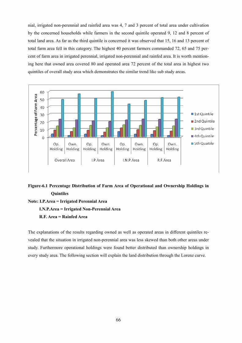
66
nial, irrigated non-perennial and rainfed area was 4, 7 and 3 percent of total area under cultivation
by the concerned households while farmers in the second quintile operated 9, 12 and 8 percent of
total land area. As far as the third quintile is concerned it was observed that 15, 16 and 13 percent of
total farm area fell in this category. The highest 40 percent farmers commanded 72, 65 and 75 per-
cent of farm area in irrigated perennial, irrigated non-perennial and rainfed area. It is worth mention-
ing here that owned area covered 80 and operated area 72 percent of the total area in highest two
quintiles of overall study area which demonstrates the similar trend like sub study areas.
Figure-6.1 Percentage Distribution of Farm Area of Operational and Ownership Holdings in
Quintiles
Note: I.P.Area = Irrigated Perennial Area
I.N.P.Area = Irrigated Non-Perennial Area
R.F. Area = Rainfed Area
The explanations of the results regarding owned as well as operated areas in different quintiles re-
vealed that the situation in irrigated non-perennial area was less skewed than both other areas under
study. Furthermore operational holdings were found better distributed than ownership holdings in
every study area. The following section will explain the land distribution through the Lorenz curve.
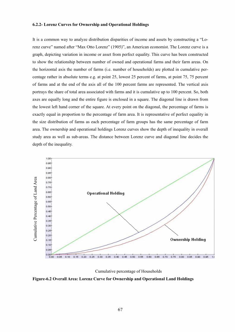
67
6.2.2- Lorenz Curves for Ownership and Operational Holdings
It is a common way to analyze distribution disparities of income and assets by constructing a “Lo-
renz curve” named after “Max Otto Lorenz” (1905)”, an American economist. The Lorenz curve is a
graph, depicting variation in income or asset from perfect equality. This curve has been constructed
to show the relationship between number of owned and operational farms and their farm areas. On
the horizontal axis the number of farms (i.e. number of households) are plotted in cumulative per-
centage rather in absolute terms e.g. at point 25, lowest 25 percent of farms, at point 75, 75 percent
of farms and at the end of the axis all of the 100 percent farms are represented. The vertical axis
portrays the share of total area associated with farms and it is cumulative up to 100 percent. So, both
axes are equally long and the entire figure is enclosed in a square. The diagonal line is drawn from
the lowest left hand corner of the square. At every point on the diagonal, the percentage of farms is
exactly equal in proportion to the percentage of farm area. It is representative of perfect equality in
the size distribution of farms as each percentage of farm groups has the same percentage of farm
area. The ownership and operational holdings Lorenz curves show the depth of inequality in overall
study area as well as sub-areas. The distance between Lorenz curve and diagonal line decides the
depth of the inequality.
Cum
ula
tive
Per
centa
ge
of
Lan
d A
rea
Cumulative percentage of Households
Figure-6.2 Overall Area: Lorenz Curve for Ownership and Operational Land Holdings
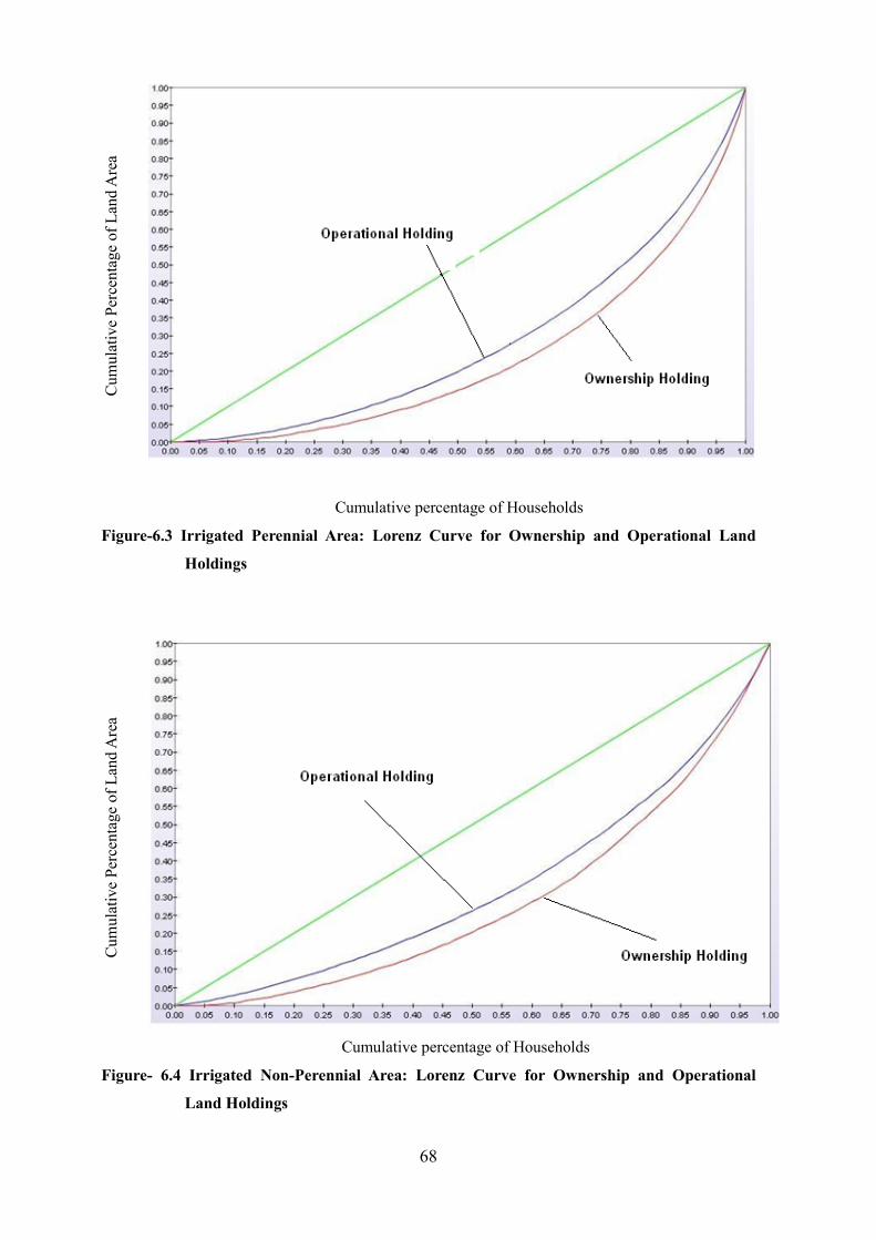
68
Cum
ula
tive
Per
centa
ge
of
Lan
d A
rea
Cumulative percentage of Households
Figure-6.3 Irrigated Perennial Area: Lorenz Curve for Ownership and Operational Land
Holdings
Cum
ula
tive
Per
centa
ge
of
Lan
d A
rea
Cumulative percentage of Households
Figure- 6.4 Irrigated Non-Perennial Area: Lorenz Curve for Ownership and Operational
Land Holdings
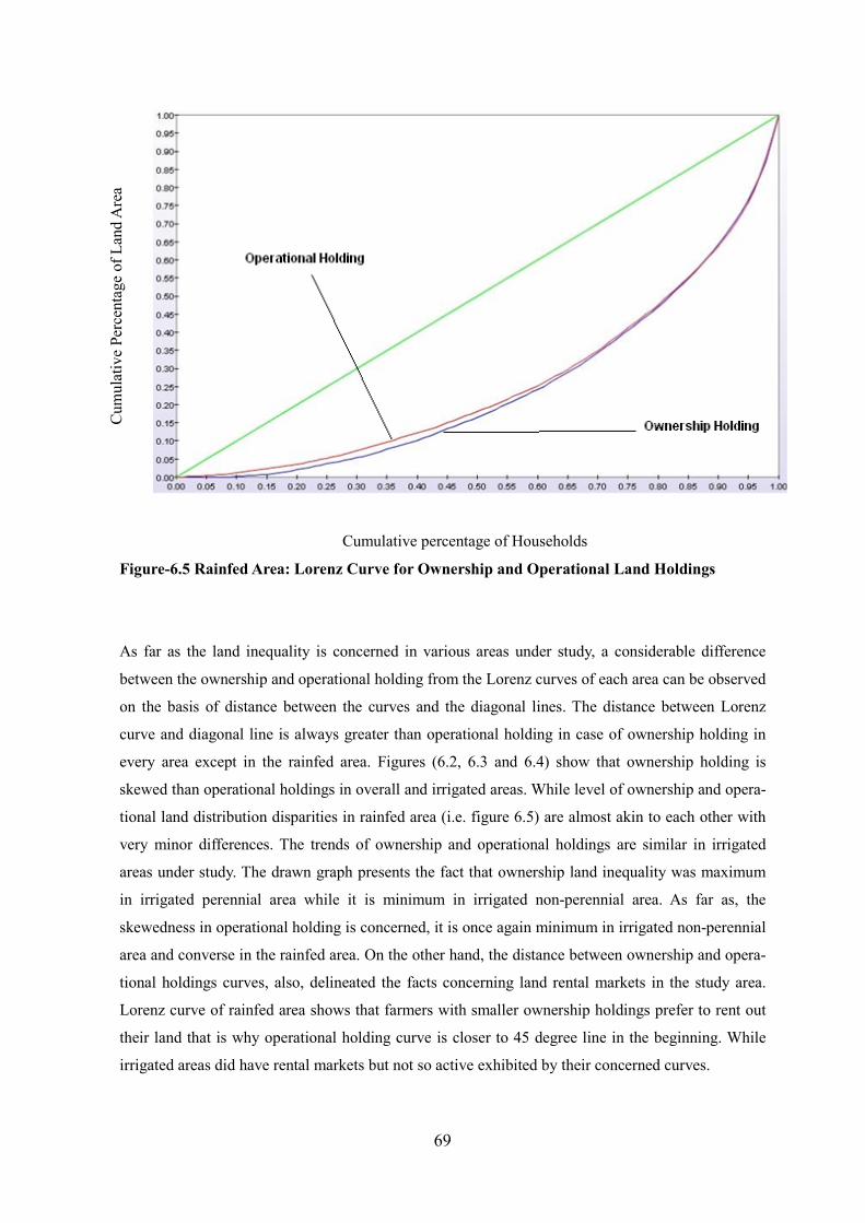
69
Cum
ula
tive
Per
centa
ge
of
Lan
d A
rea
Cumulative percentage of Households
Figure-6.5 Rainfed Area: Lorenz Curve for Ownership and Operational Land Holdings
As far as the land inequality is concerned in various areas under study, a considerable difference
between the ownership and operational holding from the Lorenz curves of each area can be observed
on the basis of distance between the curves and the diagonal lines. The distance between Lorenz
curve and diagonal line is always greater than operational holding in case of ownership holding in
every area except in the rainfed area. Figures (6.2, 6.3 and 6.4) show that ownership holding is
skewed than operational holdings in overall and irrigated areas. While level of ownership and opera-
tional land distribution disparities in rainfed area (i.e. figure 6.5) are almost akin to each other with
very minor differences. The trends of ownership and operational holdings are similar in irrigated
areas under study. The drawn graph presents the fact that ownership land inequality was maximum
in irrigated perennial area while it is minimum in irrigated non-perennial area. As far as, the
skewedness in operational holding is concerned, it is once again minimum in irrigated non-perennial
area and converse in the rainfed area. On the other hand, the distance between ownership and opera-
tional holdings curves, also, delineated the facts concerning land rental markets in the study area.
Lorenz curve of rainfed area shows that farmers with smaller ownership holdings prefer to rent out
their land that is why operational holding curve is closer to 45 degree line in the beginning. While
irrigated areas did have rental markets but not so active exhibited by their concerned curves.
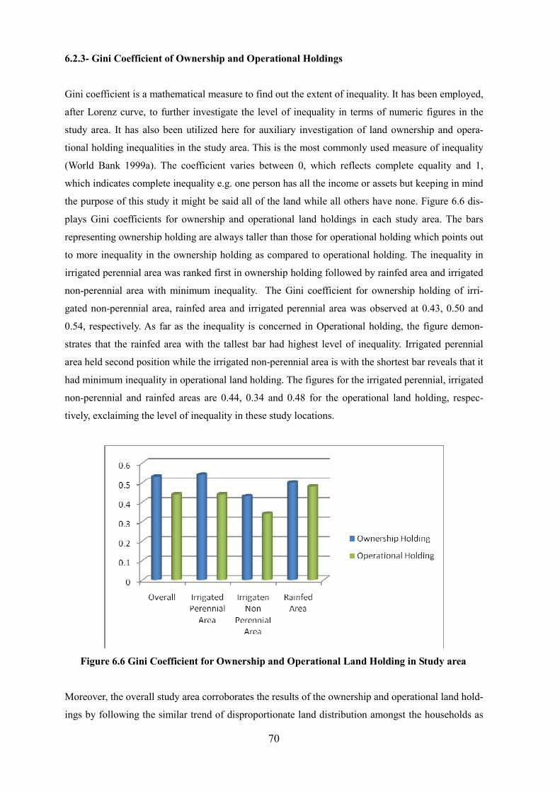
70
6.2.3- Gini Coefficient of Ownership and Operational Holdings
Gini coefficient is a mathematical measure to find out the extent of inequality. It has been employed,
after Lorenz curve, to further investigate the level of inequality in terms of numeric figures in the
study area. It has also been utilized here for auxiliary investigation of land ownership and opera-
tional holding inequalities in the study area. This is the most commonly used measure of inequality
(World Bank 1999a). The coefficient varies between 0, which reflects complete equality and 1,
which indicates complete inequality e.g. one person has all the income or assets but keeping in mind
the purpose of this study it might be said all of the land while all others have none. Figure 6.6 dis-
plays Gini coefficients for ownership and operational land holdings in each study area. The bars
representing ownership holding are always taller than those for operational holding which points out
to more inequality in the ownership holding as compared to operational holding. The inequality in
irrigated perennial area was ranked first in ownership holding followed by rainfed area and irrigated
non-perennial area with minimum inequality. The Gini coefficient for ownership holding of irri-
gated non-perennial area, rainfed area and irrigated perennial area was observed at 0.43, 0.50 and
0.54, respectively. As far as the inequality is concerned in Operational holding, the figure demon-
strates that the rainfed area with the tallest bar had highest level of inequality. Irrigated perennial
area held second position while the irrigated non-perennial area is with the shortest bar reveals that it
had minimum inequality in operational land holding. The figures for the irrigated perennial, irrigated
non-perennial and rainfed areas are 0.44, 0.34 and 0.48 for the operational land holding, respec-
tively, exclaiming the level of inequality in these study locations.
Figure 6.6 Gini Coefficient for Ownership and Operational Land Holding in Study area
Moreover, the overall study area corroborates the results of the ownership and operational land hold-
ings by following the similar trend of disproportionate land distribution amongst the households as
71
well. Figure 6.2 shows that the bar for ownership holding is taller than for operational land holding.
The Gini coefficient for ownership and operational holding is 0.53 and 0.44 for overall study area.
All of the inequality tools mentioned above found that irrigated non-perennial area had the minimum
inequality in both “ownership as well as operational land holding”. While the irrigated perennial
area stood second and the rainfed area had the maximum inequality proved by Lorenz curve and
Gini coefficient in operational holding. It is worth mentioning here that results of land ownership
distribution disparities determined by all of the tools were inline with research hypothesis of the
study. Though, operational holdings were also found skewed but skewedness was not so profound.
Furthermore, land holding was very small in all of the study locations or it can be ascribed as mar-
ginal farming which is a dilemma and to discuss it is beyond the scope of the study.
6.3- Cropping Intensity and Crop Diversity in Study Area
6.3.1- Cropping Intensity
Cropping Intensity is defined as “total cropped area in terms of total cultivated area multiplied by
100 (Government of Pakistan 2000). It indicates the extent to which the cultivated area was used for
repeated cropping in a particular year (Mahmood 2000). Figure 6.7 exposes the facts about the crop-
ping intensity of overall areas of irrigated and rainfed farming systems as well as small, medium and
large farms under study. It is noteworthy that irrigated non-perennial is at the top with highest crop-
ping intensity (i.e. 169 %), irrigated perennial area is second with 161 % and rainfed area with 153 %
lies beneath both of them. The comparison of small, medium and large farms shows that the cropping
intensity at small farms is higher than medium and large farms in every area and the large farms were
the least crop intensive in all areas, too. Furthermore, farm size categories of overall study area fol-
low the similar trend with decreasing rate of cropping intensity from small to large farms like fellow
categories of various study location. Table 6.1 delineates the detailed results regarding cropping in-
tensity in each study location along with their concerning farm size categories.
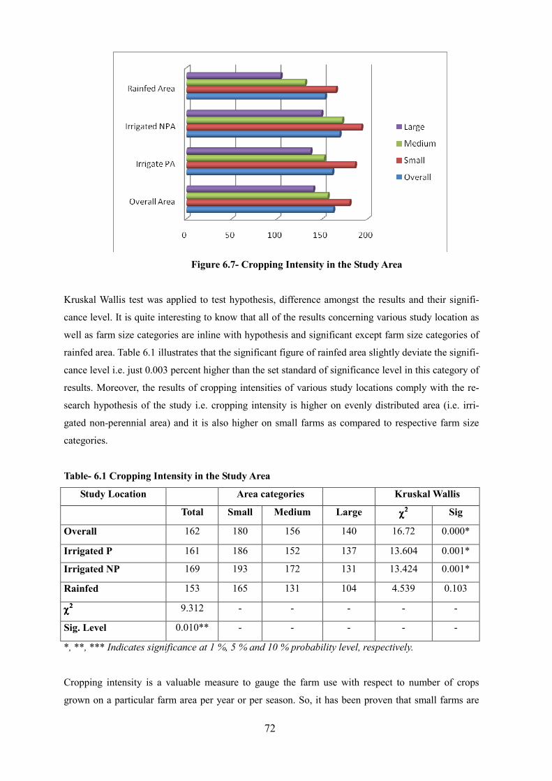
72
Figure 6.7- Cropping Intensity in the Study Area
Kruskal Wallis test was applied to test hypothesis, difference amongst the results and their signifi-
cance level. It is quite interesting to know that all of the results concerning various study location as
well as farm size categories are inline with hypothesis and significant except farm size categories of
rainfed area. Table 6.1 illustrates that the significant figure of rainfed area slightly deviate the signifi-
cance level i.e. just 0.003 percent higher than the set standard of significance level in this category of
results. Moreover, the results of cropping intensities of various study locations comply with the re-
search hypothesis of the study i.e. cropping intensity is higher on evenly distributed area (i.e. irri-
gated non-perennial area) and it is also higher on small farms as compared to respective farm size
categories.
Table- 6.1 Cropping Intensity in the Study Area
Study Location Area categories Kruskal Wallis
Total Small Medium Large χχχχ2222 Sig
Overall 162 180 156 140 16.72 0.000*
Irrigated P 161 186 152 137 13.604 0.001*
Irrigated NP 169 193 172 131 13.424 0.001*
Rainfed 153 165 131 104 4.539 0.103
χχχχ2222 9.312 - - - - -
Sig. Level 0.010** - - - - -
*, **, *** Indicates significance at 1 %, 5 % and 10 % probability level, respectively.
Cropping intensity is a valuable measure to gauge the farm use with respect to number of crops
grown on a particular farm area per year or per season. So, it has been proven that small farms are
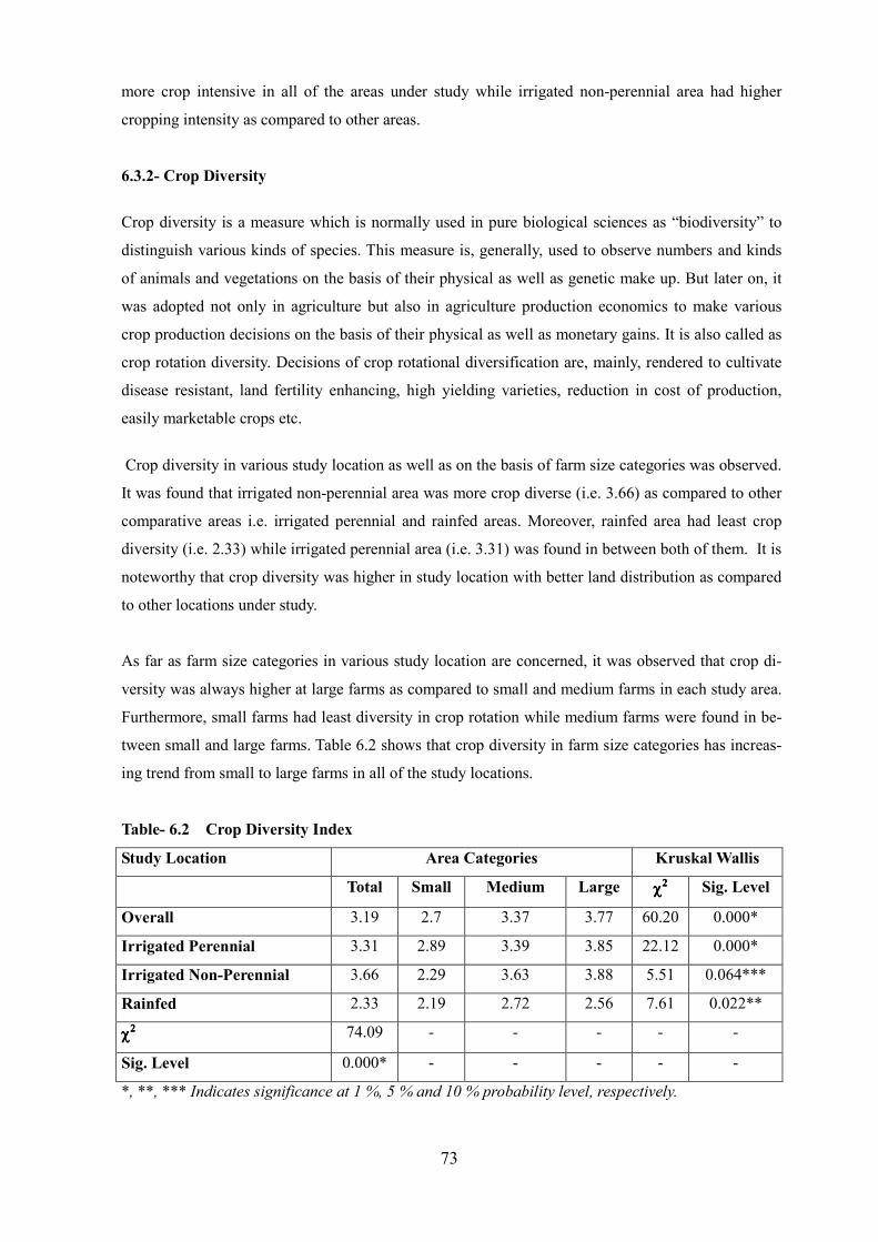
73
more crop intensive in all of the areas under study while irrigated non-perennial area had higher
cropping intensity as compared to other areas.
6.3.2- Crop Diversity
Crop diversity is a measure which is normally used in pure biological sciences as “biodiversity” to
distinguish various kinds of species. This measure is, generally, used to observe numbers and kinds
of animals and vegetations on the basis of their physical as well as genetic make up. But later on, it
was adopted not only in agriculture but also in agriculture production economics to make various
crop production decisions on the basis of their physical as well as monetary gains. It is also called as
crop rotation diversity. Decisions of crop rotational diversification are, mainly, rendered to cultivate
disease resistant, land fertility enhancing, high yielding varieties, reduction in cost of production,
easily marketable crops etc.
Crop diversity in various study location as well as on the basis of farm size categories was observed.
It was found that irrigated non-perennial area was more crop diverse (i.e. 3.66) as compared to other
comparative areas i.e. irrigated perennial and rainfed areas. Moreover, rainfed area had least crop
diversity (i.e. 2.33) while irrigated perennial area (i.e. 3.31) was found in between both of them. It is
noteworthy that crop diversity was higher in study location with better land distribution as compared
to other locations under study.
As far as farm size categories in various study location are concerned, it was observed that crop di-
versity was always higher at large farms as compared to small and medium farms in each study area.
Furthermore, small farms had least diversity in crop rotation while medium farms were found in be-
tween small and large farms. Table 6.2 shows that crop diversity in farm size categories has increas-
ing trend from small to large farms in all of the study locations.
Table- 6.2 Crop Diversity Index
Study Location Area Categories Kruskal Wallis
Total Small Medium Large χχχχ2222 Sig. Level
Overall 3.19 2.7 3.37 3.77 60.20 0.000*
Irrigated Perennial 3.31 2.89 3.39 3.85 22.12 0.000*
Irrigated Non-Perennial 3.66 2.29 3.63 3.88 5.51 0.064***
Rainfed 2.33 2.19 2.72 2.56 7.61 0.022**
χχχχ2222 74.09 - - - - -
Sig. Level 0.000* - - - - -
*, **, *** Indicates significance at 1 %, 5 % and 10 % probability level, respectively.
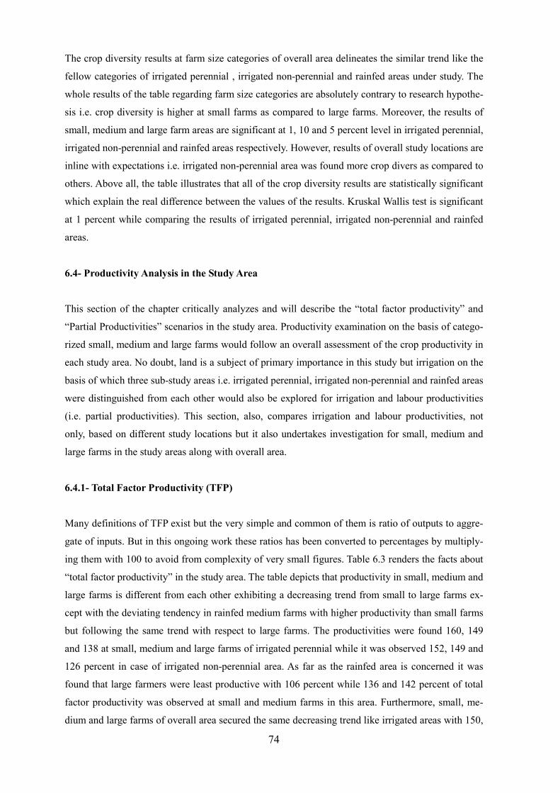
74
The crop diversity results at farm size categories of overall area delineates the similar trend like the
fellow categories of irrigated perennial , irrigated non-perennial and rainfed areas under study. The
whole results of the table regarding farm size categories are absolutely contrary to research hypothe-
sis i.e. crop diversity is higher at small farms as compared to large farms. Moreover, the results of
small, medium and large farm areas are significant at 1, 10 and 5 percent level in irrigated perennial,
irrigated non-perennial and rainfed areas respectively. However, results of overall study locations are
inline with expectations i.e. irrigated non-perennial area was found more crop divers as compared to
others. Above all, the table illustrates that all of the crop diversity results are statistically significant
which explain the real difference between the values of the results. Kruskal Wallis test is significant
at 1 percent while comparing the results of irrigated perennial, irrigated non-perennial and rainfed
areas.
6.4- Productivity Analysis in the Study Area
This section of the chapter critically analyzes and will describe the “total factor productivity” and
“Partial Productivities” scenarios in the study area. Productivity examination on the basis of catego-
rized small, medium and large farms would follow an overall assessment of the crop productivity in
each study area. No doubt, land is a subject of primary importance in this study but irrigation on the
basis of which three sub-study areas i.e. irrigated perennial, irrigated non-perennial and rainfed areas
were distinguished from each other would also be explored for irrigation and labour productivities
(i.e. partial productivities). This section, also, compares irrigation and labour productivities, not
only, based on different study locations but it also undertakes investigation for small, medium and
large farms in the study areas along with overall area.
6.4.1- Total Factor Productivity (TFP)
Many definitions of TFP exist but the very simple and common of them is ratio of outputs to aggre-
gate of inputs. But in this ongoing work these ratios has been converted to percentages by multiply-
ing them with 100 to avoid from complexity of very small figures. Table 6.3 renders the facts about
“total factor productivity” in the study area. The table depicts that productivity in small, medium and
large farms is different from each other exhibiting a decreasing trend from small to large farms ex-
cept with the deviating tendency in rainfed medium farms with higher productivity than small farms
but following the same trend with respect to large farms. The productivities were found 160, 149
and 138 at small, medium and large farms of irrigated perennial while it was observed 152, 149 and
126 percent in case of irrigated non-perennial area. As far as the rainfed area is concerned it was
found that large farmers were least productive with 106 percent while 136 and 142 percent of total
factor productivity was observed at small and medium farms in this area. Furthermore, small, me-
dium and large farms of overall area secured the same decreasing trend like irrigated areas with 150,
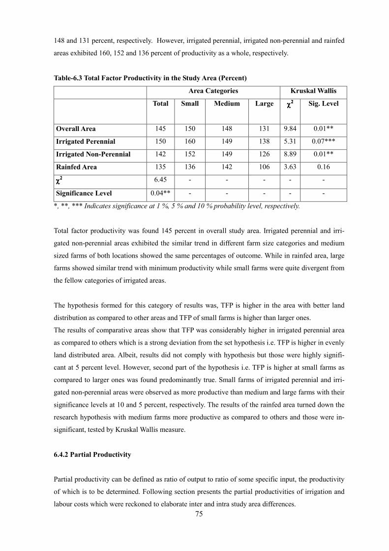
75
148 and 131 percent, respectively. However, irrigated perennial, irrigated non-perennial and rainfed
areas exhibited 160, 152 and 136 percent of productivity as a whole, respectively.
Table-6.3 Total Factor Productivity in the Study Area (Percent)
Area Categories Kruskal Wallis
Total Small Medium Large χχχχ2222 Sig. Level
Overall Area 145 150 148 131 9.84 0.01**
Irrigated Perennial 150 160 149 138 5.31 0.07***
Irrigated Non-Perennial 142 152 149 126 8.89 0.01**
Rainfed Area 135 136 142 106 3.63 0.16
χχχχ2222 6.45 - - - - -
Significance Level 0.04** - - - - -
*, **, *** Indicates significance at 1 %, 5 % and 10 % probability level, respectively.
Total factor productivity was found 145 percent in overall study area. Irrigated perennial and irri-
gated non-perennial areas exhibited the similar trend in different farm size categories and medium
sized farms of both locations showed the same percentages of outcome. While in rainfed area, large
farms showed similar trend with minimum productivity while small farms were quite divergent from
the fellow categories of irrigated areas.
The hypothesis formed for this category of results was, TFP is higher in the area with better land
distribution as compared to other areas and TFP of small farms is higher than larger ones.
The results of comparative areas show that TFP was considerably higher in irrigated perennial area
as compared to others which is a strong deviation from the set hypothesis i.e. TFP is higher in evenly
land distributed area. Albeit, results did not comply with hypothesis but those were highly signifi-
cant at 5 percent level. However, second part of the hypothesis i.e. TFP is higher at small farms as
compared to larger ones was found predominantly true. Small farms of irrigated perennial and irri-
gated non-perennial areas were observed as more productive than medium and large farms with their
significance levels at 10 and 5 percent, respectively. The results of the rainfed area turned down the
research hypothesis with medium farms more productive as compared to others and those were in-
significant, tested by Kruskal Wallis measure.
6.4.2 Partial Productivity
Partial productivity can be defined as ratio of output to ratio of some specific input, the productivity
of which is to be determined. Following section presents the partial productivities of irrigation and
labour costs which were reckoned to elaborate inter and intra study area differences.
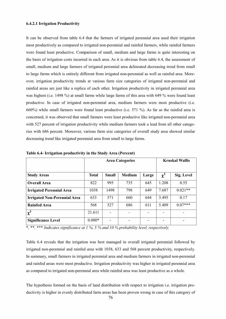
76
6.4.2.1 Irrigation Productivity
It can be observed from table 6.4 that the farmers of irrigated perennial area used their irrigation
most productively as compared to irrigated non-perennial and rainfed farmers, while rainfed farmers
were found least productive. Comparison of small, medium and large farms is quite interesting on
the basis of irrigation costs incurred in each area. As it is obvious from table 6.4, the assessment of
small, medium and large farmers of irrigated perennial area delineated decreasing trend from small
to large farms which is entirely different from irrigated non-perennial as well as rainfed area. More-
over, irrigation productivity trends at various farm size categories of irrigated non-perennial and
rainfed areas are just like a replica of each other. Irrigation productivity in irrigated perennial area
was highest (i.e. 1498 %) at small farms while large farms of this area with 649 % were found least
productive. In case of irrigated non-perennial area, medium farmers were most productive (i.e.
660%) while small farmers were found least productive (i.e. 571 %). As far as the rainfed area is
concerned, it was observed that small farmers were least productive like irrigated non-perennial area
with 527 percent of irrigation productivity while medium farmers took a lead from all other catego-
ries with 686 percent. Moreover, various farm size categories of overall study area showed similar
decreasing trend like irrigated perennial area from small to large farms.
Table 6.4- Irrigation productivity in the Study Area (Percent)
Area Categories Kruskal Wallis
Study Areas Total Small Medium Large χχχχ2222 Sig. Level
Overall Area 822 995 735 645 1.208 0.55
Irrigated Perennial Area 1038 1498 798 649 7.687 0.021**
Irrigated Non-Perennial Area 633 571 660 644 3.495 0.17
Rainfed Area 568 527 686 611 5.409 0.07***
χχχχ2222 21.611 - - - - -
Significance Level 0.000* - - - - -
*, **, *** Indicates significance at 1 %, 5 % and 10 % probability level, respectively.
Table 6.4 reveals that the irrigation was best managed in overall irrigated perennial followed by
irrigated non-perennial and rainfed area with 1038, 633 and 568 percent productivity, respectively.
In summary, small farmers in irrigated perennial area and medium farmers in irrigated non-perennial
and rainfed areas were most productive. Irrigation productivity was higher in irrigated perennial area
as compared to irrigated non-perennial area while rainfed area was least productive as a whole.
The hypothesis formed on the basis of land distribution with respect to irrigation i.e. irrigation pro-
ductivity is higher in evenly distributed farm areas has been proven wrong in case of this category of
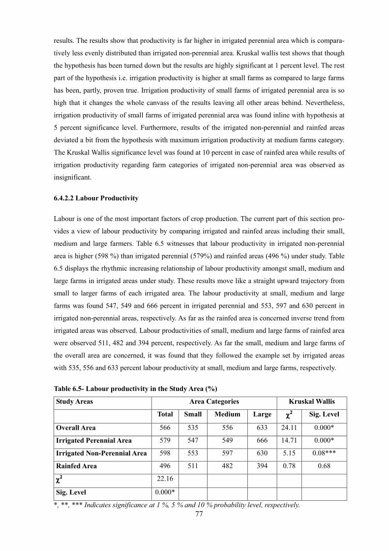
77
results. The results show that productivity is far higher in irrigated perennial area which is compara-
tively less evenly distributed than irrigated non-perennial area. Kruskal wallis test shows that though
the hypothesis has been turned down but the results are highly significant at 1 percent level. The rest
part of the hypothesis i.e. irrigation productivity is higher at small farms as compared to large farms
has been, partly, proven true. Irrigation productivity of small farms of irrigated perennial area is so
high that it changes the whole canvass of the results leaving all other areas behind. Nevertheless,
irrigation productivity of small farms of irrigated perennial area was found inline with hypothesis at
5 percent significance level. Furthermore, results of the irrigated non-perennial and rainfed areas
deviated a bit from the hypothesis with maximum irrigation productivity at medium farms category.
The Kruskal Wallis significance level was found at 10 percent in case of rainfed area while results of
irrigation productivity regarding farm categories of irrigated non-perennial area was observed as
insignificant.
6.4.2.2 Labour Productivity
Labour is one of the most important factors of crop production. The current part of this section pro-
vides a view of labour productivity by comparing irrigated and rainfed areas including their small,
medium and large farmers. Table 6.5 witnesses that labour productivity in irrigated non-perennial
area is higher (598 %) than irrigated perennial (579%) and rainfed areas (496 %) under study. Table
6.5 displays the rhythmic increasing relationship of labour productivity amongst small, medium and
large farms in irrigated areas under study. These results move like a straight upward trajectory from
small to larger farms of each irrigated area. The labour productivity at small, medium and large
farms was found 547, 549 and 666 percent in irrigated perennial and 553, 597 and 630 percent in
irrigated non-perennial areas, respectively. As far as the rainfed area is concerned inverse trend from
irrigated areas was observed. Labour productivities of small, medium and large farms of rainfed area
were observed 511, 482 and 394 percent, respectively. As far the small, medium and large farms of
the overall area are concerned, it was found that they followed the example set by irrigated areas
with 535, 556 and 633 percent labour productivity at small, medium and large farms, respectively.
Table 6.5- Labour productivity in the Study Area (%)
Study Areas Area Categories Kruskal Wallis
Total Small Medium Large χχχχ2222 Sig. Level
Overall Area 566 535 556 633 24.11 0.000*
Irrigated Perennial Area 579 547 549 666 14.71 0.000*
Irrigated Non-Perennial Area 598 553 597 630 5.15 0.08***
Rainfed Area 496 511 482 394 0.78 0.68
χχχχ2222 22.16
Sig. Level 0.000*
*, **, *** Indicates significance at 1 %, 5 % and 10 % probability level, respectively.
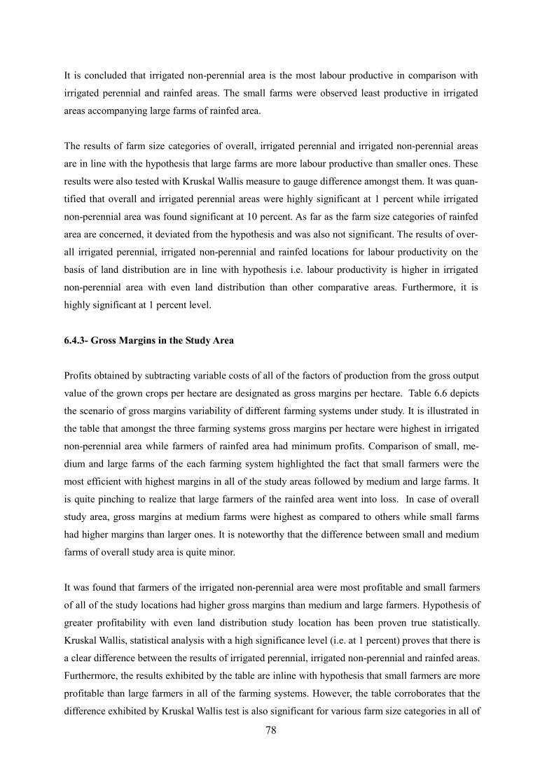
78
It is concluded that irrigated non-perennial area is the most labour productive in comparison with
irrigated perennial and rainfed areas. The small farms were observed least productive in irrigated
areas accompanying large farms of rainfed area.
The results of farm size categories of overall, irrigated perennial and irrigated non-perennial areas
are in line with the hypothesis that large farms are more labour productive than smaller ones. These
results were also tested with Kruskal Wallis measure to gauge difference amongst them. It was quan-
tified that overall and irrigated perennial areas were highly significant at 1 percent while irrigated
non-perennial area was found significant at 10 percent. As far as the farm size categories of rainfed
area are concerned, it deviated from the hypothesis and was also not significant. The results of over-
all irrigated perennial, irrigated non-perennial and rainfed locations for labour productivity on the
basis of land distribution are in line with hypothesis i.e. labour productivity is higher in irrigated
non-perennial area with even land distribution than other comparative areas. Furthermore, it is
highly significant at 1 percent level.
6.4.3- Gross Margins in the Study Area
Profits obtained by subtracting variable costs of all of the factors of production from the gross output
value of the grown crops per hectare are designated as gross margins per hectare. Table 6.6 depicts
the scenario of gross margins variability of different farming systems under study. It is illustrated in
the table that amongst the three farming systems gross margins per hectare were highest in irrigated
non-perennial area while farmers of rainfed area had minimum profits. Comparison of small, me-
dium and large farms of the each farming system highlighted the fact that small farmers were the
most efficient with highest margins in all of the study areas followed by medium and large farms. It
is quite pinching to realize that large farmers of the rainfed area went into loss. In case of overall
study area, gross margins at medium farms were highest as compared to others while small farms
had higher margins than larger ones. It is noteworthy that the difference between small and medium
farms of overall study area is quite minor.
It was found that farmers of the irrigated non-perennial area were most profitable and small farmers
of all of the study locations had higher gross margins than medium and large farmers. Hypothesis of
greater profitability with even land distribution study location has been proven true statistically.
Kruskal Wallis, statistical analysis with a high significance level (i.e. at 1 percent) proves that there is
a clear difference between the results of irrigated perennial, irrigated non-perennial and rainfed areas.
Furthermore, the results exhibited by the table are inline with hypothesis that small farmers are more
profitable than large farmers in all of the farming systems. However, the table corroborates that the
difference exhibited by Kruskal Wallis test is also significant for various farm size categories in all of
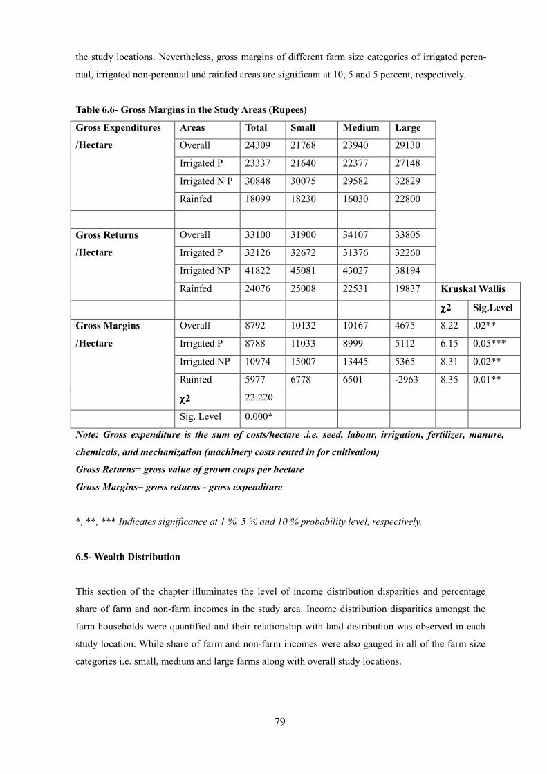
79
the study locations. Nevertheless, gross margins of different farm size categories of irrigated peren-
nial, irrigated non-perennial and rainfed areas are significant at 10, 5 and 5 percent, respectively.
Table 6.6- Gross Margins in the Study Areas (Rupees)
Gross Expenditures
/Hectare
Areas Total Small Medium Large
Overall 24309 21768 23940 29130
Irrigated P 23337 21640 22377 27148
Irrigated N P 30848 30075 29582 32829
Rainfed 18099 18230 16030 22800
Gross Returns
/Hectare
Overall 33100 31900 34107 33805
Irrigated P 32126 32672 31376 32260
Irrigated NP 41822 45081 43027 38194
Rainfed 24076 25008 22531 19837 Kruskal Wallis
χχχχ2 Sig.Level
Gross Margins
/Hectare
Overall 8792 10132 10167 4675 8.22 .02**
Irrigated P 8788 11033 8999 5112 6.15 0.05***
Irrigated NP 10974 15007 13445 5365 8.31 0.02**
Rainfed 5977 6778 6501 -2963 8.35 0.01**
χχχχ2 22.220
Sig. Level 0.000*
Note: Gross expenditure is the sum of costs/hectare .i.e. seed, labour, irrigation, fertilizer, manure,
chemicals, and mechanization (machinery costs rented in for cultivation)
Gross Returns= gross value of grown crops per hectare
Gross Margins= gross returns - gross expenditure
*, **, *** Indicates significance at 1 %, 5 % and 10 % probability level, respectively.
6.5- Wealth Distribution
This section of the chapter illuminates the level of income distribution disparities and percentage
share of farm and non-farm incomes in the study area. Income distribution disparities amongst the
farm households were quantified and their relationship with land distribution was observed in each
study location. While share of farm and non-farm incomes were also gauged in all of the farm size
categories i.e. small, medium and large farms along with overall study locations.
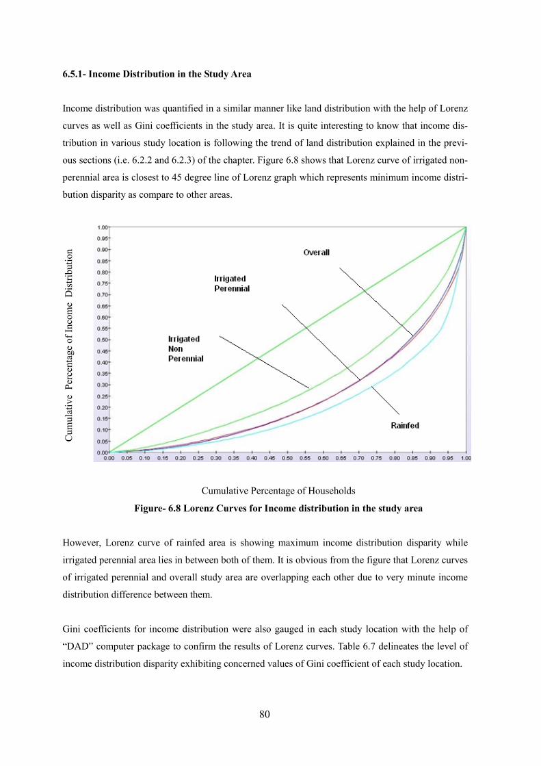
80
6.5.1- Income Distribution in the Study Area
Income distribution was quantified in a similar manner like land distribution with the help of Lorenz
curves as well as Gini coefficients in the study area. It is quite interesting to know that income dis-
tribution in various study location is following the trend of land distribution explained in the previ-
ous sections (i.e. 6.2.2 and 6.2.3) of the chapter. Figure 6.8 shows that Lorenz curve of irrigated non-
perennial area is closest to 45 degree line of Lorenz graph which represents minimum income distri-
bution disparity as compare to other areas.
Cum
ula
tive
Per
centa
ge
of
Inco
me
Dis
trib
uti
on
Cumulative Percentage of Households
Figure- 6.8 Lorenz Curves for Income distribution in the study area
However, Lorenz curve of rainfed area is showing maximum income distribution disparity while
irrigated perennial area lies in between both of them. It is obvious from the figure that Lorenz curves
of irrigated perennial and overall study area are overlapping each other due to very minute income
distribution difference between them.
Gini coefficients for income distribution were also gauged in each study location with the help of
“DAD” computer package to confirm the results of Lorenz curves. Table 6.7 delineates the level of
income distribution disparity exhibiting concerned values of Gini coefficient of each study location.
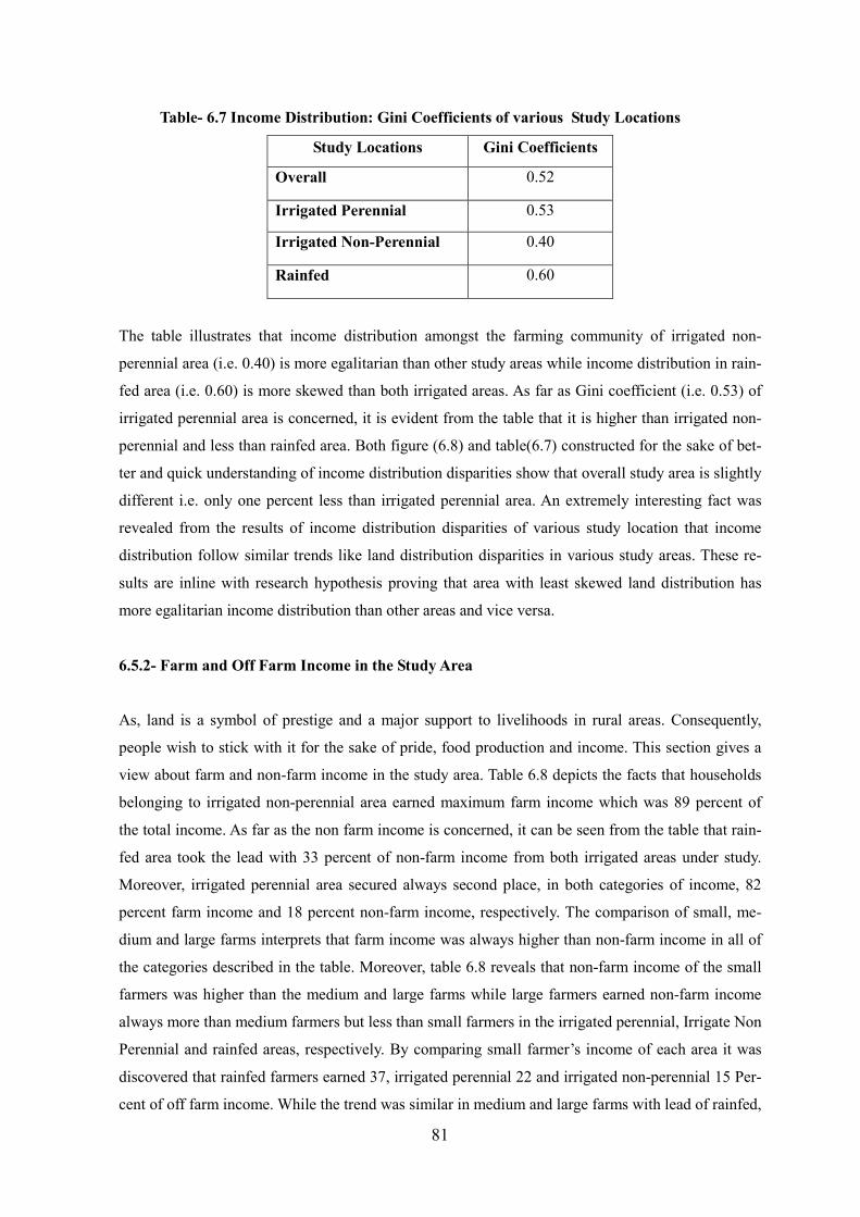
81
Table- 6.7 Income Distribution: Gini Coefficients of various Study Locations
Study Locations Gini Coefficients
Overall 0.52
Irrigated Perennial 0.53
Irrigated Non-Perennial 0.40
Rainfed 0.60
The table illustrates that income distribution amongst the farming community of irrigated non-
perennial area (i.e. 0.40) is more egalitarian than other study areas while income distribution in rain-
fed area (i.e. 0.60) is more skewed than both irrigated areas. As far as Gini coefficient (i.e. 0.53) of
irrigated perennial area is concerned, it is evident from the table that it is higher than irrigated non-
perennial and less than rainfed area. Both figure (6.8) and table(6.7) constructed for the sake of bet-
ter and quick understanding of income distribution disparities show that overall study area is slightly
different i.e. only one percent less than irrigated perennial area. An extremely interesting fact was
revealed from the results of income distribution disparities of various study location that income
distribution follow similar trends like land distribution disparities in various study areas. These re-
sults are inline with research hypothesis proving that area with least skewed land distribution has
more egalitarian income distribution than other areas and vice versa.
6.5.2- Farm and Off Farm Income in the Study Area
As, land is a symbol of prestige and a major support to livelihoods in rural areas. Consequently,
people wish to stick with it for the sake of pride, food production and income. This section gives a
view about farm and non-farm income in the study area. Table 6.8 depicts the facts that households
belonging to irrigated non-perennial area earned maximum farm income which was 89 percent of
the total income. As far as the non farm income is concerned, it can be seen from the table that rain-
fed area took the lead with 33 percent of non-farm income from both irrigated areas under study.
Moreover, irrigated perennial area secured always second place, in both categories of income, 82
percent farm income and 18 percent non-farm income, respectively. The comparison of small, me-
dium and large farms interprets that farm income was always higher than non-farm income in all of
the categories described in the table. Moreover, table 6.8 reveals that non-farm income of the small
farmers was higher than the medium and large farms while large farmers earned non-farm income
always more than medium farmers but less than small farmers in the irrigated perennial, Irrigate Non
Perennial and rainfed areas, respectively. By comparing small farmer’s income of each area it was
discovered that rainfed farmers earned 37, irrigated perennial 22 and irrigated non-perennial 15 Per-
cent of off farm income. While the trend was similar in medium and large farms with lead of rainfed,
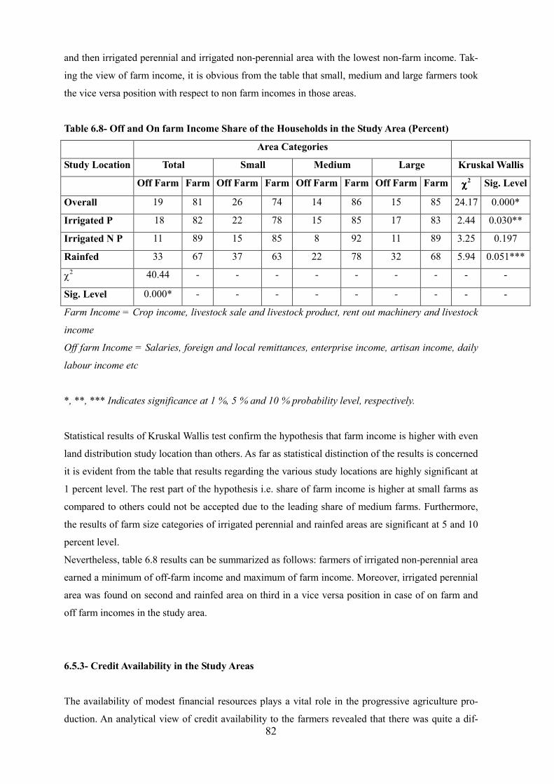
82
and then irrigated perennial and irrigated non-perennial area with the lowest non-farm income. Tak-
ing the view of farm income, it is obvious from the table that small, medium and large farmers took
the vice versa position with respect to non farm incomes in those areas.
Table 6.8- Off and On farm Income Share of the Households in the Study Area (Percent)
Area Categories
Study Location Total Small Medium Large Kruskal Wallis
Off Farm Farm Off Farm Farm Off Farm Farm Off Farm Farm χχχχ2 Sig. Level
Overall 19 81 26 74 14 86 15 85 24.17 0.000*
Irrigated P 18 82 22 78 15 85 17 83 2.44 0.030**
Irrigated N P 11 89 15 85 8 92 11 89 3.25 0.197
Rainfed 33 67 37 63 22 78 32 68 5.94 0.051***
χ2 40.44 - - - - - - - - -
Sig. Level 0.000* - - - - - - - - -
Farm Income = Crop income, livestock sale and livestock product, rent out machinery and livestock
income
Off farm Income = Salaries, foreign and local remittances, enterprise income, artisan income, daily
labour income etc
*, **, *** Indicates significance at 1 %, 5 % and 10 % probability level, respectively.
Statistical results of Kruskal Wallis test confirm the hypothesis that farm income is higher with even
land distribution study location than others. As far as statistical distinction of the results is concerned
it is evident from the table that results regarding the various study locations are highly significant at
1 percent level. The rest part of the hypothesis i.e. share of farm income is higher at small farms as
compared to others could not be accepted due to the leading share of medium farms. Furthermore,
the results of farm size categories of irrigated perennial and rainfed areas are significant at 5 and 10
percent level.
Nevertheless, table 6.8 results can be summarized as follows: farmers of irrigated non-perennial area
earned a minimum of off-farm income and maximum of farm income. Moreover, irrigated perennial
area was found on second and rainfed area on third in a vice versa position in case of on farm and
off farm incomes in the study area.
6.5.3- Credit Availability in the Study Areas
The availability of modest financial resources plays a vital role in the progressive agriculture pro-
duction. An analytical view of credit availability to the farmers revealed that there was quite a dif-
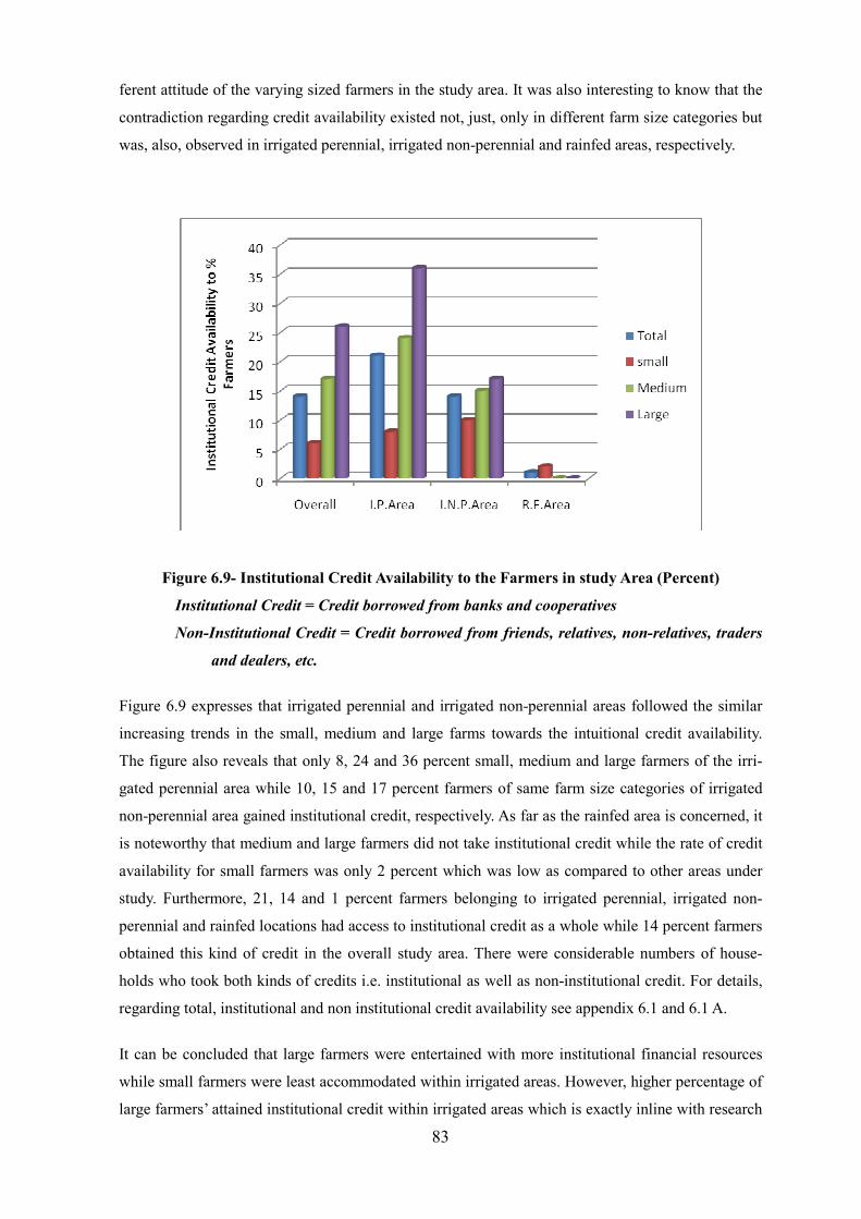
83
ferent attitude of the varying sized farmers in the study area. It was also interesting to know that the
contradiction regarding credit availability existed not, just, only in different farm size categories but
was, also, observed in irrigated perennial, irrigated non-perennial and rainfed areas, respectively.
Figure 6.9- Institutional Credit Availability to the Farmers in study Area (Percent)
Institutional Credit = Credit borrowed from banks and cooperatives
Non-Institutional Credit = Credit borrowed from friends, relatives, non-relatives, traders
and dealers, etc.
Figure 6.9 expresses that irrigated perennial and irrigated non-perennial areas followed the similar
increasing trends in the small, medium and large farms towards the intuitional credit availability.
The figure also reveals that only 8, 24 and 36 percent small, medium and large farmers of the irri-
gated perennial area while 10, 15 and 17 percent farmers of same farm size categories of irrigated
non-perennial area gained institutional credit, respectively. As far as the rainfed area is concerned, it
is noteworthy that medium and large farmers did not take institutional credit while the rate of credit
availability for small farmers was only 2 percent which was low as compared to other areas under
study. Furthermore, 21, 14 and 1 percent farmers belonging to irrigated perennial, irrigated non-
perennial and rainfed locations had access to institutional credit as a whole while 14 percent farmers
obtained this kind of credit in the overall study area. There were considerable numbers of house-
holds who took both kinds of credits i.e. institutional as well as non-institutional credit. For details,
regarding total, institutional and non institutional credit availability see appendix 6.1 and 6.1 A.
It can be concluded that large farmers were entertained with more institutional financial resources
while small farmers were least accommodated within irrigated areas. However, higher percentage of
large farmers’ attained institutional credit within irrigated areas which is exactly inline with research
84
hypothesis of the study which was formed based on the theory. While farm size categories of rainfed
area showed deviation from hypothesis. Moreover, higher percentage of irrigated perennial farmers
took more institutional credit as compared to other study areas. The results regarding institutional
credit availability for overall study locations deviated from the research hypothesis i.e. farmers of
even land distribution take more institutional credit as compare to other areas.
6.6- Evidence of Inverse Relationship: Productivity and Factors of Production
This section helps to expose the kind of relationship whether it was direct or inverse, between the
output per hectare and various factors of production used to till the land in study area. Particular
attention was given to the explanatory factors which directly affect the crop productivity per hectare
to attain the maximum rationale results and, consequently, can also foster to give workable policy
recommendations in the end of the study. Table 6.9 presents the outcome of Cobb-Douglas produc-
tion function (i.e. log-log function) which was utilized for the sake of data analysis. The results
quoted in table 6.9 verified the negative relationship between operational holdings and output per
hectare by a negative sign in all of the areas along with overall area under study. Surprisingly, credit
availability per hectare had a similar inverse relationship with output per hectare in all of the areas.
As far as the age of the households head is concerned, it is illustrated by table 6.9, productivity per
hectare was found directly proportional to the increasing years of households head life span in irri-
gated non-perennial area while it was inversely proportional in the irrigated perennial, rainfed as
well as Overall study area. It is evident from the table, contrary to the age of household head, the
family size or number of household members took on different trends towards crop productivity per
hectare. The rise in number of family members also enhanced productivity in positive direction in
irrigated perennial and rainfed area while in irrigated non-perennial area ascending family size set
the productivity towards diminishing trend. Nevertheless, crop productivity increased with increase
in the rest of the factors of production including, labour, irrigation, intermediate inputs, education of
the household head, percentage of family workers in agriculture sector and own tubewell in all of
the areas under study. It is illustrated in the table that labour (man-days) and intermediate inputs had
the strongest productivity raising impact in all of the areas while some factors of production had
mixed coincidence of strong and weaker relationship with productivity in various areas under study.
It was an astonishing revelation that non-farm income and tractor ownership made no differences in
the productivity per hectare in irrigated perennial area.
Table 6.9 says that there are only two explanatory variables (i.e. labour investment and intermediate
inputs) which are not only significant but also highly significant with maximum effect on productiv-
ity in all of the areas. Though operational holding is showing inverse relationship but this relation-
ship is significantly weaker in each study area. The elasticities were not so vibrant and can reduce
productivity at the level of 0.05, 0.07 and 0.07 percent with 1 percent increase in operational holding
in command in irrigated perennial, irrigated non-perennial and rainfed areas respectively. The credit
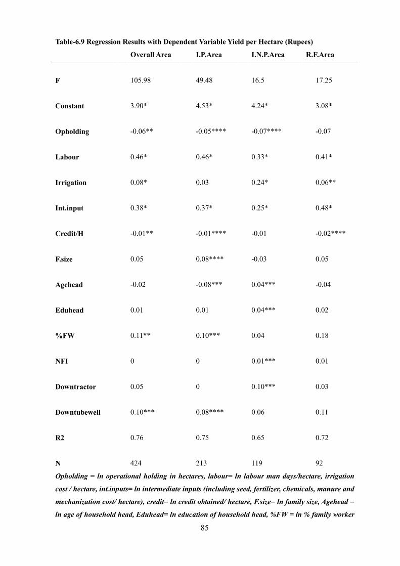
85
Table-6.9 Regression Results with Dependent Variable Yield per Hectare (Rupees)
Overall Area I.P.Area I.N.P.Area R.F.Area
F 105.98 49.48 16.5 17.25
Constant 3.90* 4.53* 4.24* 3.08*
Opholding -0.06** -0.05**** -0.07**** -0.07
Labour 0.46* 0.46* 0.33* 0.41*
Irrigation 0.08* 0.03 0.24* 0.06**
Int.input 0.38* 0.37* 0.25* 0.48*
Credit/H -0.01** -0.01**** -0.01 -0.02****
F.size 0.05 0.08**** -0.03 0.05
Agehead -0.02 -0.08*** 0.04*** -0.04
Eduhead 0.01 0.01 0.04*** 0.02
%FW 0.11** 0.10*** 0.04 0.18
NFI 0 0 0.01*** 0.01
Downtractor 0.05 0 0.10*** 0.03
Downtubewell 0.10*** 0.08**** 0.06 0.11
R2 0.76 0.75 0.65 0.72
N 424 213 119 92
Opholding = ln operational holding in hectares, labour= ln labour man days/hectare, irrigation
cost / hectare, int.inputs= ln intermediate inputs (including seed, fertilizer, chemicals, manure and
mechanization cost/ hectare), credit= ln credit obtained/ hectare, F.size= ln family size, Agehead =
ln age of household head, Eduhead= ln education of household head, %FW = ln % family worker
86
in agriculture production, NFI= ln non-farm income of households, Downtractor= ln dummay
variable own tractor, Downtubewell = ln dummay variable own tubewell.
*, **, *** Indicates significance at 1 %, 5 % and 10 % probability level, respectively.
availability per hectare also reduces productivity with the rate of 0.01, 0.01 and 0.02 percent with 1
percent increase in it in irrigated perennial, irrigated non-perennial and rainfed areas. As far as the
labour and irrigation is concerned , it was found that 1 percent addition in labour man days increase
0.46, 0.33 and 0.41 percent while 1 percent enhancement in irrigation cost per hectare augment
0.03, 0.24 and 0.06 percent in productivity per hectare in irrigated perennial, irrigated non-perennial
and rainfed area , respectively. The 1 percent addition in intermediate inputs enhance productivity
with the rate of 0.37, 0.25, and 0.48 percent, and own tubewell helped to rise 0.08, 0.06 and 0.11
percent of productivity in irrigated perennial and irrigated non-perennial and rainfed area, respec-
tively.
The results of the different farming systems showed that inverse relationship between irrigation pro-
ductivity and operational holding do exist in all of the areas which is also online with hypothesis of
the study that inverse relationship exists between farm size and productivity in all study locations.
Interestingly, IR exists in all of the study locations regardless of irrigation infrastructure, water
availability and land distribution disparities scenario of the study area. Furthermore, results of IR are
significant at 10 percent in overall study area while those are significant at 20 percent in both irri-
gated areas and insignificant in rainfed area. Irrigated perennial and irrigated non-perennial area
contained 8 variables with significant results each, while rainfed area had few variables with signifi-
cant results i.e. only 4. As far as the overall area is concerned, 7 variables were found with signifi-
cant results in it.
The significance level limit of regression results has been set at 20 percent which might be unusual
but this notion has been scrounged from a famous inverse relationship study (i.e. Cornia 1985).
The chapter briefs that the results of land distribution disparity delineated strong skewedness in
ownership holdings while operational holdings were found, comparatively, better distributed. Fur-
thermore, operational holdings were observed as least skewed in irrigated non-perennial area fol-
lowed by irrigated perennial and rainfed study locations. The results of income distribution in the
study area revealed that it followed the similar trends with minimum income distribution disparities
in irrigated non-perennial area while rainfed area was found most skewed. It is quite interesting to
know that most of the results of the study were akin to ranking of land distribution disparities in
various study locations. Various indicators of the study showed mixed results supporting small and

87
large farms but those were more inclined towards small farms. It is noteworthy that most of the re-
search hypotheses were found true whether those were formed in favour of small and large farms
depending on kind of indicators. Moreover, it was observed that inverse relation between farm size
and productivity existed in all of the study locations including overall study area. But the presence
of IR was found as weak with small coefficients of operational holdings.
88
CHAPTER-7
DISCUSSION
The results of the study presented in chapter 6 are being discussed in this chapter. The findings of the study
are supported by the previous literature. The difference to observe same or similar aspects of this subject
are also dealt with. A lot of dimensions have been thrashed, and it is hoped that some of them are new. But
also some of older ideas with innovative factors are incorporated. The discussion mainly concentrates upon
the land distribution and productivity analysis in three different farming systems i.e. irrigated perennial,
irrigated non-perennial and rainfed areas. The results would be discussed on the basis of land distribution
disparities in three study locations while the discussion will also focus on farm size categories (i.e. small
and large farms). The chapter has been organized in a format i.e. a) inverse relationship restated b) land
distribution c) land distribution, input levels and yields d) land distribution and factor productivity e) land
distribution, cropping intensity and diversity f) small versus large farms and at the end of the chapter g)
inverse relationship is concluded.
7.1- Inverse Relationship Restated
Small farms are more productive than larger ones is designated as inverse relationship. It is very famous
and perhaps most debated issue in the field of agriculture production economics since last many decades.
Though a lot of economist has proved its validity but this idea was turned down by a lot of its opponents
keeping it still unresolved leaving the potential for further investigation. In the early 20th century a Russian
economist (Chayanov 1926) was the first one who hypothesized the idea of productivity dominance of
small farms over the larger ones with the better endowments of the family labour force. Unfortunately, he
was mistreated by the Russian socialists with the fear of hurting socialism. Although his book was trans-
lated into English in 1966 but in the modern literature an Indian development economist Sen (1962, 1966)
is considered as a founder of this idea on the basis of his publication on this issue. It might be expressed as
renaissance of an ideology. It has been a hot debate for development economists and sociologists for dec-
ades with many new interventions of its research and study aspects and discoveries in analytical tools to
arrive at some common conclusion but in vain. After five decades, it is still a very significant part of devel-
opment economics research. It is worth mentioning that redistributive land reform is one of its very strong
implications which paved the way for redistribution of lands by grabbing agricultural lands from big landed
elites and bestowing it to smaller peasants in many countries of the world. The burgeoning population of
the earth and increasing food demands in the world has once again diverted the attention of the researcher
and policy makers towards this issue which results in brain storming of many reputed institutions of USA,
UK, Germany and many others. This study is also such a kind of an endeavor to observe productivity
differentials on various farm sizes and to give policy recommendation for the policy makers to act accor-
89
dingly to produce more food for humanity. In addition, various locations were studied on the basis of their
land distribution disparities employing various indicators to observe the differences. These both approaches
of study i.e. land distribution disparity and farm size patterns ultimately lead to similar kinds of policy
recommendations.
7.2- Land Distribution
Mal-distribution of land and its ill impacts has been presented regarding Pakistan in chapter 1 and in detail
in chapter 4 in the light of previous literature including local, country and cross country studies carried out
indigenously or funded by international organizations like World Bank, International Monetary Fund (IMF)
and International Food Policy Research Institute (IFPRI). Furthermore, positive impacts of even land
distribution have been referred to in the same chapter in the form of rapid economic growth as well as
human development in different countries. Figure 7.1 illustrates the ailing and healthy impacts of uneven
and even land distribution, respectively, on the basis of previous research as well as undergoing study.
Land distribution being a prime object of the study was gauged by more than one measure (i.e. quin-
tiles, Lorenz curve and Gini coefficient) to avoid any kind of bias in the study but results were quite
similar. To ignore tedious details, just two measures has been discussed here i.e. land distribution by
quintile and Gini coefficient. It is worth mentioning here that land distribution disparities were ob-
served on the basis of two core criteria i.e. ownership holding as well as operational holdings and it
would be quite favourable to demonstrate that the whole study was focused upon operational holdings
in spite of ownership holdings in the study area. It is noteworthy that the study area was comprised of
overall small holdings or it could be referred to as marginal farmers. According to the descriptive sta-
tistics average land holdings in each area either ownership or operational holding was not found more
than four hectares and it was less than 3 hectares in the overall study area. As far as per capita land
ownership is concerned, it was found to be less than 0.5 hectares per person in each area including
overall area under study. Furthermore, the trend is similar regarding per capita operational holdings.
The results of quintile show that the 20 percent farmers of lowest quintile own only 2, 4 and 2 percent
of total area in irrigated perennial, irrigated non-perennial and rainfed area, respectively. Furthermore,
20 percent farmers of second quintiles own 6, 9 and 8 percent of total area while farmers of third and
fourth quintiles own 12, 15 and 14, and 20, 24 and 24 percent of total area, respectively. While 60, 48
and 52 percent of total area was owned by top 20 percent of the farmers in irrigated perennial, irri-
gated non-perennial and rainfed area. The quintile based analysis of the land distribution exclaims that
land distribution is not evenly distributed in the study area and a wide gap between the percentage area
owned by top and lowest quintiles explores the land distribution disparities in the study area.
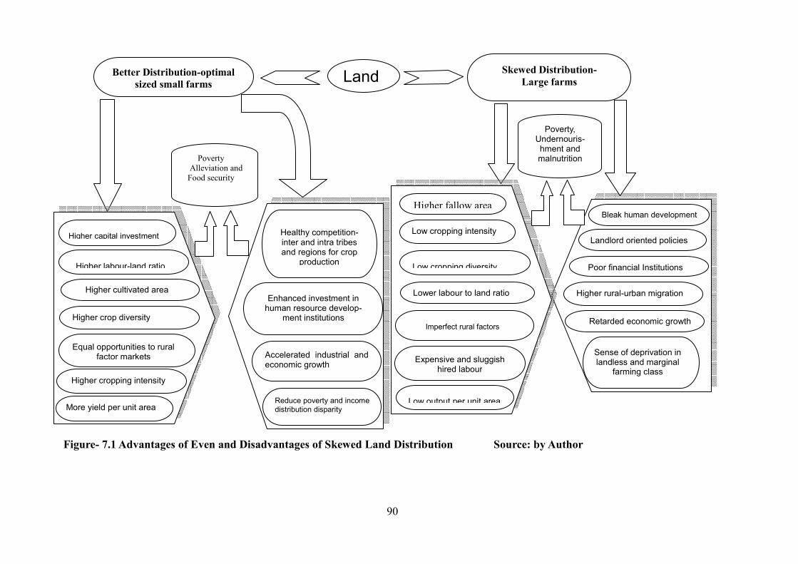
90
Better Distribution-optimal
sized small farms
Higher capital investment
Higher labour-land ratio
Higher cultivated area
Higher crop diversity
Equal opportunities to rural factor markets
Higher cropping intensity
More yield per unit area
Bleak human development
Landlord oriented policies
Poor financial Institutions
Higher rural-urban migration
Retarded economic growth
Sense of deprivation in landless and marginal
farming class
Land Skewed Distribution-
Large farms
Poverty, Undernouris-hment and malnutrition
Higher fallow area
Low cropping intensity
Low cropping diversity
Lower labour to land ratio
Imperfect rural factors
Expensive and sluggish hired labour
Low output per unit area
Poverty
Alleviation and
Food security
Healthy competition-inter and intra tribes and regions for crop
production
Enhanced investment in human resource develop-
ment institutions
Accelerated industrial and economic growth
Reduce poverty and income distribution disparity
Figure- 7.1 Advantages of Even and Disadvantages of Skewed Land Distribution Source: by Author
91
As far as the operational land holding is concerned, the results exhibited similar trends through quintile
analysis but a bit better than ownership holdings in each area under study. Nevertheless, this simple arith-
metic was needed to be confirmed with some scientific measure. So, World Bank recommended “Gini
coefficient” accompanied by some others to know the exact level of land distribution disparities in the
study area. The results obtained for ownership holdings were categorized in an ascending order of land
distribution disparities in various areas i.e. least skewed irrigated non-perennial ( 0.43), then rainfed (0.50)
and irrigated perennial area was found (0.54) with most distorted land distribution. The pattern of opera-
tional holdings considering the same order with respect to Gini coefficient were found as, irrigated non-
perennial area (0.34), irrigated perennial area (0.44) and rainfed area (0.48). The difference between the
Gini of ownership and operational holdings explains existence of land rental markets in both irrigated
areas. It is noteworthy that the area with comparatively even ownership holdings (i.e. irrigated non-
perennial area) has better land rental markets which made its operational holdings relatively equal as com-
pared to rest of the study locations. The most skewed ownership holdings in irrigated perennial area might
be a cause of land market imperfections but it is compensated perhaps with year round water availability in
this area. But it is a matter of further investigation to get acquaintance with this fact. Moreover, due to
unavailability of irrigation infrastructure and skewed land distribution severely hampers land rental markets
in rainfed area. The variations in ownership and operational holdings Gini is very small i.e. 0.02 in this
area. The differences between ownership and operational holdings can easily be understood by visualizing
Lorenz curves of each study location in chapter 6. During land distribution disparity analysis very few
cases of large holdings were omitted from the analysis to draw a real picture of the results. The chapters of
the study incorporated as preamble site that land distribution in the country is more skewed as compared to
the area under study. Neither land reform efforts nor green revolution could rectify this phenomenon in
Pakistan. A bulk of literature concerning farm size studies ignored ownership holdings and had concen-
trated upon operational holdings to examine the relationship of farm size and productivity e.g. Berry and
Cline (1979), Dyer (1997), Cornia (1985), Bhalla (1979) Thapa (2007) Unal (2008) etc.
Uneven land distribution, in Pakistan, like most of the developing countries is a direct consequence of
imperialism and colonialism. A lot has been written on the significance of land but skewed land distribution
is really a blight which not only impedes the overall agriculture productivity (Vollrath 2006) but it also
curtails the mental maturity, human resource development and, above all, tarnishes self esteem of the small
peasants. Skewed land distribution, marginal farming and landless agriculture is a cause of poverty and
food insecurity in Pakistan (Anwar et al. 2004). A number of land reforms attempts were undertaken in
1959, 1972 and 1977 but desired results could not be achieved due to lacunae in promulgations as well as
in implementation processes. The depth of the issue is so grave that many nations of the globe had to in-
itiate different kinds of land reforms in order to get rid of big estates which worked as an impetus in their
development e.g. Japan, South Korea, Taiwan, and China. Now a day, Vietnam is tracking the same path.
As the whole study has been founded on land distribution, so, it was felt mandatory to discuss foremost
92
land distributional matters in the study area. Furthermore, it is illustrated that the current land distribution
disparity is in accordance with many previous studies which include Mahmood (2000), Sain (1974), Sal-
man and Moinuddin (1980), Rehman (1986), Nazir (1999), and Eastwood et al. (2004). They all and many
others observed mal-distribution of land in their studies.
7.3- Land distribution, Input Levels and Yield
A great deal of studies followed the appraisal of investment costs linking up yields per unit area by stan-
dardizing various farm sizes but non of them (as far as I know) pursued on the basis of actual existence of
land distribution except Vollrath (2006) who worked on macro data in a cross country study. Most studies
are based on macro data while a substantial amount of them are also available on micro level data, too. But
none of the researcher recorded the differentiation of the areas like in this study except Heltberg (1998)
worked on two distinguished locations i.e. irrigated and rainfed area in Pakistan.
The results under discussion in this section of the chapter have been elucidated in chapter six. It has been
exposed that land distribution was least skewed in irrigated non-perennial area and rainfed area contained
most distorted and irrigated perennial areas was in between both of them. A certain relationship of labour
(in man days), irrigation and intermediate inputs (i.e. seed, fertilizer, chemical & manure, mechanization)
costs with yield per hectare was found in each area. It was assessed that a very strong positive relationship
existed between overall costs of production, better land distribution and outcomes which might be a great
stimulus for the farmers to invest more in an environment of pure competition. It is very interesting to
mention here, regardless of materials as well as human beings, every factor was intensively cast to achieve
higher yield per hectare. Therefore, it achieved more revenue according to the land distribution level which
has always been the objective of any entrepreneur. It can better and simply be explained by quoting that
better distribution of land would enhance the investment capacity and inspire motivation in the farmers to
grow more and produce in bulk. It helps change imperfect factors market towards pure competition. Irri-
gated non-perennial area, being evenly distributed than other areas, was most intensively ploughed with
more labour man days not only with overall but with family as well as hired persons than both other areas.
Furthermore, all of the factors of productions were found more intensively utilized in irrigated non-
perennial area while least investment had been found in rainfed area. As far as the yield per hectare is
concerned, once again irrigated non-perennial area was found more productive than any other region under
study. While irrigated perennial area was found in between both other areas according to its land distribu-
tion status. Furthermore, bigger gross margins were also achieved by the cultivators of irrigated non-
perennial area and the similar trends had been observed from rest of the areas under study i.e. irrigated
perennial area on second while rainfed area was found on lowest level with respect to gross margins of the
field crops.
93
Investment on factors of production and the consequent yield per hectare exhibit some certain implications
in the presence of land distribution level in each area which would be elaborated in conclusions and rec-
ommendation part of the study. However, the hypothesis of factors market imperfection can be better
understood and might be confirmed in the outcome of present results and discussion in this section of the
chapter. In addition, even land distribution may provide an opportunity to get rid of monopoly or oligopoly
and to create the environment of pure competition in the local factor markets. The aforementioned results
and discussions come closer to the, already, work done by Heltberg (1998, 1996), Unal (2008) Cornia
(1985) and Vollrath (2006).
7.4- Land Distribution and Factor Productivity
The results regarding crop productivity, and labour and irrigation productivities were determined as total
factor productivity and partial factor productivities in various areas, has been discussed here in the light of
land distribution levels. It could be interesting to integrate farm size categories together with productivities
but it was avoided due to the overlapping hazards of so many things together which might create ambiguity
for the reader. Nevertheless, the facts regarding various farm sizes categories will be discussed in a separate
section as it is one of the most significant aspects of this study.
The aforementioned indicators i.e. yields, gross margins etc per hectare reveal the superiority of irrigated
non-perennial area, conceivably, on the basis of better land distribution over both other areas. Productivity
facts showed little deviation from the preceding results. Though, the difference is quite petty but it can not
be ignored rather to put forth some strong rationale. The total factor productivity puts output in monetary
terms against costs of all of the factors of productions which include labour and irrigation costs as well.
Total factor productivity in irrigated non-perennial area is lower than irrigated perennial area but higher
than rainfed area. In the irrigated non-perennial area with the input of 1 rupee farmers attained 1.42 rupees
in return while with the same level of inputs in irrigated perennial area and rainfed area 1.50 and 1.35
rupees were earned. The difference is due to the decisive role of irrigation expenditures. The upcoming
section (i.e. 7.6) will reveal the very fact of this difference of total factor and irrigation productivities
between irrigated non-perennial area and irrigated perennial area. As the irrigated non-perennial farmers
had to spend for full six months on tubewell irrigation while in irrigated perennial area canal irrigation was
enjoyed for the whole year and occasional deficiencies were overcome by the conjunctive use of tubewells.
Furthermore the rainfed farmers had to either rely upon tubewells or rain. Unfortunately, 2001 and 2002
were extreme drought years and rainfed farmers had to rely more and more on pumped irrigation. Partial
productivities of irrigation and labour revealed different trends. Irrigation followed the same trend like the
total factor productivity while labour productivity was highest in irrigated non-perennial and least in
rainfed area. Albeit, there is no alternative of cheap irrigation but wise use and management of labour
helped to diminish the total factor productivity gap between irrigated perennial and non-perennial areas.
94
It is believed that the total factor and irrigation productivity differentials in the two irrigated areas were due
to the varying irrigation costs whereas those differences had been minimized due to better land distribution
in irrigated non-perennial area along with other supporting factors of production. It is concluded that ceteris
paribus, level of land distribution along with prudent labour use would play decisive role in productivity
enhancing mechanism.
7.5- Land Distribution, Cropping Intensity and Crop Diversity
The results regarding cropping intensities and cropping diversity of the farmers were elaborated in chapter-
6. These two measures discussed here keeping the distinction of each area in mind along with their land
distribution. It was found, once again like previous results, apart from total factor productivity and irriga-
tion productivity, irrigated non-perennial area asserted maximum cropping intensity as compared to other
areas under study. While irrigated perennial area stood second and rainfed area like always acquired last
position. These results (regarding cropping Intensities) were found in accordance with their level of land
distribution as the distribution gets nearer equality which means a lower Gini coefficient. Nevertheless, it
can be explained more precisely by expressing it in terms of direct (∞) relationship between land distribu-
tion and cropping intensity which implies that better land distribution connotes higher cropping Intensity,
more revenue, more food security and less poverty in the concerned areas. Crop diversity of the farmers in
different areas was observed and its results were also delineated in chapter 6. Crop diversity followed the
similar trends like many other indicators of the study i.e. cropping intensity, gross margins, input costs,
yield per hectare etc. Crop diversity was higher in irrigated non-perennial area which had better land distri-
bution as compared to other areas under study.
The results of the aforementioned three farming systems distinguished in the context of irrigation infra-
structure and seasonal as well as permanent availability of water for crop production were discussed in
detail to understand the differences. It was inferred that, though, irrigation plays a vital role in agriculture
production and crop productivity per unit area but even land distribution is also important which affects
each and every measure in the favour of land tillers. No doubt, irrigation plays a crucial role in agriculture
production but even land distribution can also help to get rid of hunger, mal-nutrition and food insecurity
from the earth. Moreover, successful land distribution efforts can augment the tilling intensity of the pea-
sants and ending absentee landlordism which will increase land use intensity, cropping intensity and better
per unit output of land area. That is why it can be implicated that land reforms must be promulgated and
implemented with full political will which could establish egalitarian rural society but those land reforms
should not be used to victimize political rivals as was done during 1970s in Pakistan (Jalal 1995).
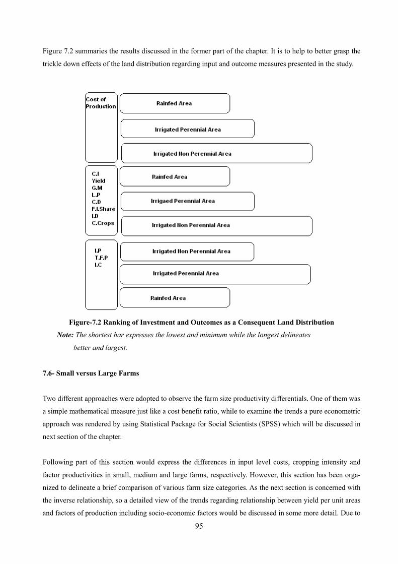
95
Figure 7.2 summaries the results discussed in the former part of the chapter. It is to help to better grasp the
trickle down effects of the land distribution regarding input and outcome measures presented in the study.
Figure-7.2 Ranking of Investment and Outcomes as a Consequent Land Distribution
Note: The shortest bar expresses the lowest and minimum while the longest delineates
better and largest.
7.6- Small versus Large Farms
Two different approaches were adopted to observe the farm size productivity differentials. One of them was
a simple mathematical measure just like a cost benefit ratio, while to examine the trends a pure econometric
approach was rendered by using Statistical Package for Social Scientists (SPSS) which will be discussed in
next section of the chapter.
Following part of this section would express the differences in input level costs, cropping intensity and
factor productivities in small, medium and large farms, respectively. However, this section has been orga-
nized to delineate a brief comparison of various farm size categories. As the next section is concerned with
the inverse relationship, so a detailed view of the trends regarding relationship between yield per unit areas
and factors of production including socio-economic factors would be discussed in some more detail. Due to
96
the smaller holdings in the area small, medium and large farms segregation was only less than 2, 2-4 and
greater than 4 hectares respectively, which might be a draw back of the study.
As far as the factors (inputs) are concerned, seed, fertilizer and manure, and mechanization costs were
always in rhythmic descending order with decreasing rate per unit area from small to large farms in each
study location. But, a very little difference of mechanization cost on large farms which was a bit higher
than medium farms in irrigated perennial category. While costs incurred on chemicals were all the times
higher in larger farms and rather low on smaller ones. The difference is so enormous that it changes the
ultimate fate of the total inputs in the end and overall input level of larger farms exceeds the smaller ones. It
unveils that fact that small farmers prefer weeding manually instead to spray expensive weedicides and
herbicides. Moreover, the labour cost intensity was found highest on smaller farms followed by medium
and large farms in irrigated perennial and irrigated non-perennial areas. The rainfed area deviated from the
trend in a reverse order i.e. higher labour was used at large farms and than other both farm size categories
while small farms utilized minimum hired labour. The descriptive part of chapter three shows that average
land ownership holdings in rainfed area was very small which might be the reason for small farmers house-
holds to find some alternative earning opportunities. This phenomenon would have reduced labour intensity
at small farms of rainfed area. Moreover, unavailability of irrigation is also a dilemma which turned their
attention to non-farm livelihood. However, labour intensity on the various farm size categories was accord-
ing to the, previously, proven theory in irrigated areas. Small farmers are more sensitive to their food re-
quirements and their lacking capacity to purchase motivates them to work more on the farm. Furthermore,
comparison of farm size categories confirmed the sequence of highest costs intensity of irrigation on small
sized farms followed by large and then medium farms in irrigated non-perennial and rainfed areas. Moreo-
ver, irrigation cost intensity was found highest at large farms and minimum at small farms in irrigated
perennial area. Water use intensity (i.e. cost of irrigation) in irrigated perennial area showed that small
farms use their irrigation more wisely. They better manage and do their best to grow maximum with mini-
mum water. Amongst the three categories of farms i.e. small, medium and large it was observed that gen-
erally small farms were most factor intensive as compared to large farms in all of the study areas except
chemicals in all and irrigation costs in irrigated perennial area. The logic to spend more on the factors of
production might lie in the price differentials due to imperfect factors markets (Heltberg 1998, Unal 2008).
Secondly, small farmers are more sensitive towards their survival and they work more, and use more inputs
per unit area. Higher mechanization costs incurred by the smaller farmers are due to the fact that they lack
machinery and they have to rent in, in the sowing seasons along with harvesting and threshing times as
well. Moreover, seed is, mostly, used from the home stored inventories. It is also used more intensively but
some times it reduces final output due to higher use than recommended by the agriculture department. The
dominance of factor intensity on small farms is inline with the theory concerning inverse relationship
debate.
97
Comparison of cropping intensity amongst small, medium and large farms shows that it is higher at small
farms in all study locations i.e. irrigated perennial, irrigated non-perennial and rainfed areas. Moreover, the
trend is same at small farm size categories of overall study area. These results are inline with previous
theory mentioned by various scientists (Kiani 2008, Bardhan 1973, Griffin et al. 2002). Small farmers are
upon the teetering brinks of poverty and food security. They grow more numbers of crops per annum leav-
ing no or minimum land fallow to escape hunger. Higher cropping intensity on small farms is one of the
most weighted arguments of the proponents in favour of inverse relationship. Small farmers are least labour
productive in both irrigated and overall study areas due to the fact that small peasants devote maximum of
their labour force by employing far more man labour days than medium and large farms. According to
some economists’ utilization of large amount of labour makes fundamental difference of yield per unit area
between small and large farms (Sen 1962, 1966, 1999, Unal 2008, Cornia 1985). It is normally done in land
scarce and labour abundant countries with skewed land distribution. As far as the labour productivity of
various farm size groups of rainfed area is concerned, it was observed that it was in reverse order of the
other study locations. Due to lack of public irrigation infrastructure people do not, overwhelmingly, depend
on agriculture production. That is why, it was found that percentage share of non-farm income was signifi-
cantly higher in this area as compared to other areas.
It is worth mentioning here that similarities were observed in various farm size categories concerning total
factor productivity i.e. it decrease with increase in farm size in irrigated perennial and irrigated non-
perennial area. As it has been discussed earlier small farmers are more conscious about their food security
due to limited buying capacity and they work hard and also strive for crop per drop to secure more food. In
addition, medium farms of rainfed has higher total factor productivity than other categories but the differ-
ence between small and medium farms is not wide in all of the study locations including irrigated and
rainfed areas. As far as irrigation productivity is concerned, it was observed that in case of overall and
irrigated perennial areas the trend is same i.e. decreasing from small to large. Furthermore, irrigated non-
perennial and rainfed area have similar trends with higher irrigation productivities at medium farms follow-
ing large and then small farms. Due to very small average land holdings, the difference between farm size
categories is not too big and it will not be surprising if for a moment medium farms are annexed with
smaller ones in rainfed and irrigated non-perennial area. Consequently, it can be said that large farms use
more irrigation and those are less productive than small farmers. Irrigation availability results comply with
the work of Haq (2007) i.e. water distribution is skewed with reference to farm size holdings.
7.7- Inverse Relationship Concluded
The productivity dominance of small farms over large farms is designated as “inverse relationship” (IR). A
detailed view was presented in chapter- 4 regarding IR and the previous section of the chapter corroborated
facts which were determined with the help of simple mathematical tools and discussed with reference to
98
this study. This section of the study has been organized to discuss the regression results concerning farm
size productivity. Log-log econometric function was utilized to observe the impacts of explanatory va-
riables on yield per hectare. This study is different from the previous studies in the sense that impact of
different deterministic as well socio-economic variables on the dependent variables was examined which
has not ever been studied earlier. Furthermore, IR was quantified on the basis of three different farming
systems with micro level data which is a kind of new effort in this sector of research.
The negative relationship between yield per unit area as dependent variable and farm size along with many
others as regressor was determined. A negative relationship, between farm size and productivity, was
proved in all of the study areas which confirm the several studies like Unal (2008), Thapa (2007), Mat-
chaya (2007), Heltberg (1996 and 1998), Benjamin (1995) and Carter (1984) but it is noteworthy that its
existence was very weak. As far as its significance level is concerned, it was found that IR in irrigated areas
was significant at 20 percent. The rationale of weak IR and lower level significance might be the high share
of very small holding in the study area which is in line with Cornia’s (1985) cross country study; he
dropped three countries ( according to him) due to marginal holdings hurting the final result of the
study.
It is evident from the regression results that labour man days and intermediate inputs which included seed,
fertilizer plus manure, chemical and mechanization costs played an important role in the farm size produc-
tivity. The positive signs, in each area, of these both factors illustrate that farm yield increase with increase
in labour man days and intermediate inputs investments. “More yields with more labour input” has been
accepted in the development economics literature and these farms are termed “family farms”. Though,
family labour could not be incorporated directly as a single entity due to multicollinearity problems but was
utilized together with hired labour in the regression analysis. However, it is confirmed from the field visits
as well as from the crude data on hand family labour played a key role in farming in the study area. It is
very interesting to know that labor man days and intermediate inputs per hectare were highly significant i.e.
at 1 percent level which confirms that these results can easily be generalized in any situation and any place.
Moreover, the regression results concerning more labour cause higher yield per unit area is inline with the
famous dualistic labour hypothesis of formers studies (Bhalla 1979, Sen 1962, 1966).
Output per hectares and irrigation cost results showed that more irrigations attains higher yield per hectare
(positive signs in every area). It is really interesting to note that irrigated perennial area where water is
available for whole year from the public infrastructure its relationship with yield is insignificant and least
strong as compared to other areas under study. Irrigation cost contributed to yield more than any other area
and highly significant in irrigated non-perennial area. The reason might be restricted availability of water
for 6 months, farmers have to spend more on irrigation and, consequently, they gained more yield with
better management. As far as impact of Irrigation cost on output is concerned in rainfed area, it was ob-
99
vious from the regression results that its contribution is higher than irrigated perennial area but lower than
irrigated non-perennial area, and interestingly, it is significant at 10 percent level. Moreover similar results
were obtained for overall study area i.e. positive relationship between yield and irrigation cost and highly
significant. Though land distribution is better in irrigated non-perennial area but, in general, overall farm
size is small in all of the study areas, so it would not be irrational to term these farms as family farms. In
irrigated perennial areas water is as cheaper just as attained for granted from the public infrastructure,
resultantly, it is poorly managed, and farmers of irrigated non-perennial area and rainfed areas have to
expend higher so they strive hard to grow crop per drop.
Credit per hectare was also tested against the yield. A negative relationship between credit and output per
hectare was found. The examination of overall study area revealed its significance at 10 percent level while
irrigated perennial and rainfed areas at 20 percent, respectively. This negative relationship may have two
kinds of explanation. First, the decreasing amount of credit stimulates output per hectare in the positive
direction and productivity is reduced with increase in borrowing level. Due to the lack of financial institu-
tions, illiteracy, small holdings, tedious documentations, fear of confiscation etc farmers borrow from local
merchants and money lenders at higher interest rates but they lack capacity to return. Consequently, they
have to sell their produce to the lenders at low rates than market prices which severely reduce their overall
revenue and they have to become a part of the vicious circle of poverty.
The relationship of the share of non-farm income with productivity had two various dimensions in different
study areas. As far as the overall and irrigated perennial areas are concerned, the regression results showed
that there is, absolutely, no relationship between non-farm income and productivity but in case of irrigated
non-perennial and rainfed areas the relationship is positive. However, the impact on productivity is meager
i.e. just 0.01 value of non-farm income which means that a 1 percent increase in off-farm income would
enhance 0.01 percent output per hectare in both study areas. Moreover, this relationship is significant in
case of irrigated perennial area at 10 percent while it is insignificant in rainfed area. By recalling, on and
off-farm income module in the results section, the economies of the concerned rural areas were not diversi-
fied, as a lion’s share of income was attributed to farm income. People rely on farm income either as self-
cultivator or farm worker. Secondly due to smaller holdings in the area, family member don’t use their off-
farm earning to the farm operations and they might prefer to keep both types of income for different pur-
poses. The employment module (i.e. appendix 3.2) of chapter-3 revealed facts and figures about the em-
ployed labour force in the concerning districts of the study area with distinguishing figures of labour force
participation in various sectors. The agricultural sector absorbs most of the labour force followed by con-
struction work. Land is a sign of prestige and farming communities considers any work other than agricul-
ture as petty job. So they get stuck up with agriculture.
100
As far as socio-economic or efficiency factors of production i.e. family size, age, and education of house-
hold head are concerned, negative relationship between increasing age of household head and productivity
was observed in overall, irrigated perennial and rainfed areas which is in accordance with the previous
studies (Unal 2008). It seems quite logical because aged people impair their decision making capability as
well as resistant to new technologies and methods of innovative agricultural practices. While in irrigated
non-perennial area, age delineated positive impact on farm productivity. The descriptive section in chapter
five gave the glimpse of average ages of the household heads, and the households’ head of the irrigated
non-perennial areas were found younger than both other areas of comparison that might be reason of posi-
tive relationship between productivity and age in this area.
A positive relationship between productivity and education of households head was observed in all of the
study areas including overall area, but this relationship was found significant only in irrigated non-
perennial area at 10 percent level. For the time being keeping significance of the results aside, it is a natural
phenomenon that education promotes and polishes the capabilities which is known as a human resource
development these days. It has been observed that the relationship is positive but it is not as strong as it
should be. However, the results are in line with previous studies (World Bank1999, Asadullah and Rehman
2006). Family size and farm productivity were directly proportional in irrigated perennial, rainfed and
overall areas while irrigated non-perennial area had negative relationship with Productivity per unit area.
The positive relationship between productivity and family size is similar to previous studies. It is insignifi-
cant in overall and rainfed area while it is significant in irrigated perennial area. Though the relationship is
positive, its impact is not strong.
It is concluded that the study proves the existence of inverse relationship i.e. small farmers are more pro-
ductive than large farmers in the whole study area. Albeit, the relationship is not very strong due to preva-
lence of perhaps marginal land holdings along with some other reasons which needs to be further investi-
gated. The empirical work done in three different areas also exposed the better agriculture production with
better land distribution location compared to others might be a proxy of inverse relationship.
101
CHAPTER-8
CONCLUSIONS AND RECOMMENDATIONS
The prepositions mentioned in chapter one regarding unequal land distribution in Pakistan and general
views concerning land distribution and farm size productivity presented in chapter four seem true
based on the results of the undergoing study. However, skewed land distribution presented in chapter
two supported by macro level data is confirmed by the study but, unfortunately, size of holdings was
observed very small in the study area. Most of the research hypotheses formed on the basis of theory
were found true while few of the results contradicted from their hypothesis. Nevertheless, matter of
land distribution disparity, its impacts on farm size productivity were addressed especially to gauge the
differences in various farming systems according to the objectives of the study. Moreover, cropping
intensity, crop diversity, yield, gross margins, total and partial factor productivities per hectare and
income distribution disparities were examined for varying environments of land distribution situation.
Furthermore, different indicators were also assessed to quantify the better gains in various farm size
categories i.e. small, medium and large farms. In the end; stylized fact of “inverse relationship” was
also studied to observe its existence in various farming systems. However, aftermaths of the study
including recommendations for the policy makers are being described in this brief chapter. Land and
water play pivotal roles in the agriculture sector. The following are the main conclusions extracted
from the study.
8.1- Conclusions
1- Land distribution was found skewed in ownership holdings but the level of inequality was not so
profound in operational holdings. Rather it pointed to the marginal or subsistence farm sizes in the
study area. The contribution of ownership holdings in the study was, only, uptil distribution disparities
while operational holdings were utilized to quantify all of the study indicators. On the basis of differ-
ences in land distribution in three areas i.e. irrigated perennial, irrigated non-perennial and rainfed
areas, the following conclusions were drawn,
a) Inequality in operational land holdings was graded as, least in irrigated non-perennial, inter-
mediate in irrigated perennial and most pronounced in rainfed area. Moreover, the average
operational holdings were higher in irrigated non-perennial area than both others. However,
ownership holdings were found highly skewed in all of the study locations. Land ownership
inequality was maximum in irrigated perennial and was minimum in irrigated non-perennial
area while rainfed area was found in between both of them. It is very interesting revelation
that the area ( i.e. irrigated non-perennial) with better land distribution had healthier land
102
markets as compared to others which means more farmers participate in leasing in and out ac-
tivities to grow more and to earn more. Furthermore, irrigated perennial area also had good
land markets perhaps due to year round water availability but it could not succeed irrigated
non-perennial area. Unfortunately, land markets were highly imperfect in rainfed area due to
lack of irrigation infrastructure and skewed ownership land holdings.
b) Although the cheaper irrigation was available in irrigated perennial area year-round but due
to better land distribution and equality in irrigated non-perennial area the competition
amongst farmers was high for greater yields and net profits. So, they applied more inputs and
achieved higher yields and gross margins per unit area than both others. While rainfed area
produced least accompanying the minimum gross margins per hectare.
c) Irrigated non-perennial area was found more labour productive than both other areas. Higher
family labour as well as hired labour man days were put in. This mean that better distribution
of land creates more work opportunities in the area and it may help to reduce rural-urban mi-
gration in search of work which results in slums in the cities. It was also observed that irri-
gated non-perennial area was leading in the share of farm income followed by irrigated pe-
rennial and rainfed areas.
d) Irrigation productivity per unit area was higher in irrigated perennial area than irrigated non-
perennial and rainfed areas which was an outcome of cheaper water availability. Moreover,
the farmers of irrigated perennial area used tubewells, too, for conjunctive water use as a sup-
plement which resulted in poor water management. Total factor productivity was also found
higher in irrigated perennial area than irrigated non-perennial and rainfed areas. Actually,
small farm irrigation and total factor productivity of irrigated perennial area makes a signifi-
cant difference in the overall productivities of this area. It is believed that this difference was
due to lower costs of water, although, there might be some other factors involved which
should be the topic of further research.
e) Cropping intensity is another very important indicator to assess the intensiveness of farming
activity on a certain farm in some particular area along with grown number of crops per an-
num. Incredibly, cropping intensity was higher in irrigated non-perennial area as compared to
other areas. Moreover, these three locations were also studied for crop diversity. It was found
that crop diversity was also higher in irrigated non-perennial area than other areas under
study. Cropping intensity and crop diversity, both, were least in rainfed area while irrigated
perennial area was found in between both other study locations regarding these measures.
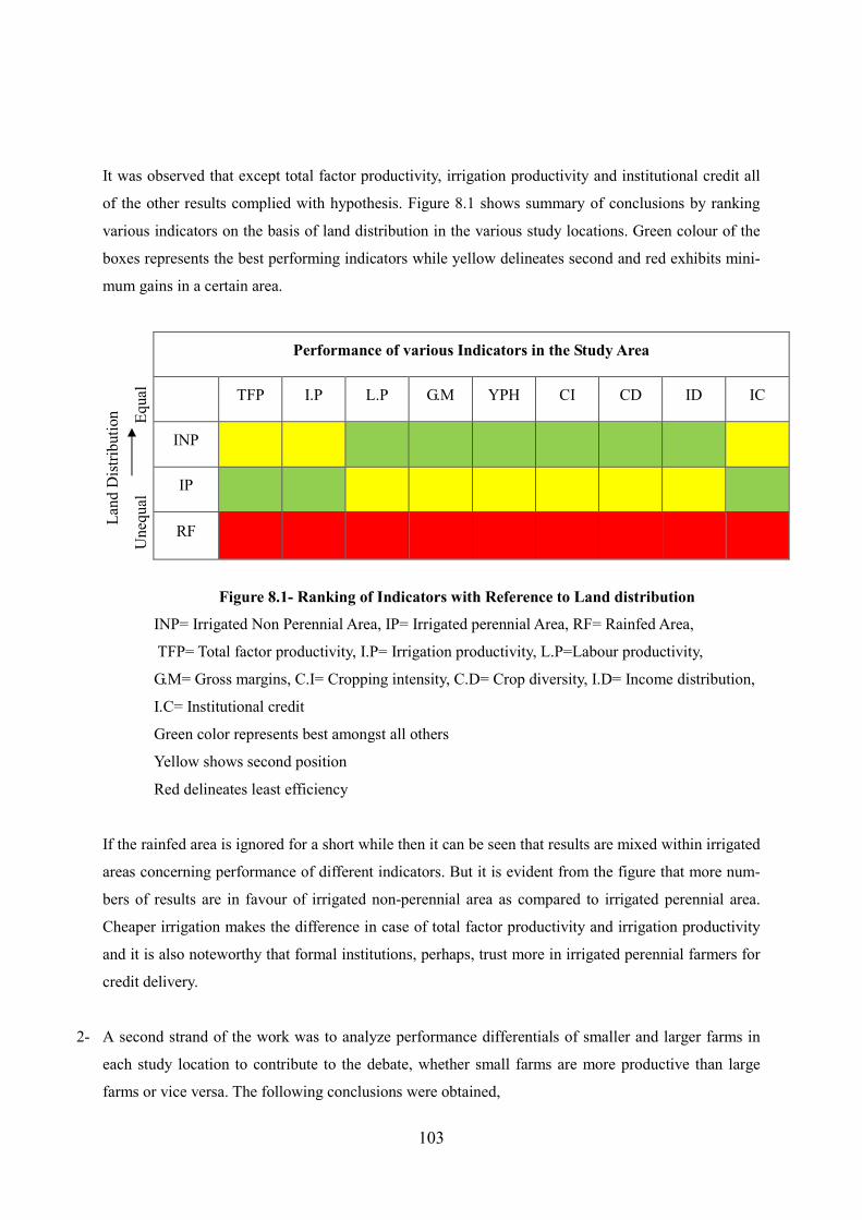
103
It was observed that except total factor productivity, irrigation productivity and institutional credit all
of the other results complied with hypothesis. Figure 8.1 shows summary of conclusions by ranking
various indicators on the basis of land distribution in the various study locations. Green colour of the
boxes represents the best performing indicators while yellow delineates second and red exhibits mini-
mum gains in a certain area.
Performance of various Indicators in the Study Area
Lan
d D
istr
ibuti
on
Uneq
ual
E
qual
TFP I.P L.P G.M YPH CI CD ID IC
INP
IP
RF
Figure 8.1- Ranking of Indicators with Reference to Land distribution
INP= Irrigated Non Perennial Area, IP= Irrigated perennial Area, RF= Rainfed Area,
TFP= Total factor productivity, I.P= Irrigation productivity, L.P=Labour productivity,
G.M= Gross margins, C.I= Cropping intensity, C.D= Crop diversity, I.D= Income distribution,
I.C= Institutional credit
Green color represents best amongst all others
Yellow shows second position
Red delineates least efficiency
If the rainfed area is ignored for a short while then it can be seen that results are mixed within irrigated
areas concerning performance of different indicators. But it is evident from the figure that more num-
bers of results are in favour of irrigated non-perennial area as compared to irrigated perennial area.
Cheaper irrigation makes the difference in case of total factor productivity and irrigation productivity
and it is also noteworthy that formal institutions, perhaps, trust more in irrigated perennial farmers for
credit delivery.
2- A second strand of the work was to analyze performance differentials of smaller and larger farms in
each study location to contribute to the debate, whether small farms are more productive than large
farms or vice versa. The following conclusions were obtained,
104
a- A comparison between farm size categories based on level of cropping intensity was underta-
ken. It was found that cropping intensity on small farms of every study location was higher
than large farms. Furthermore, small farms of overall study area also excel in cropping intensi-
ty as compared to large farms. However, crop diversity was found higher at large farms in all
of the study locations.
b- The view of overall input use proved that large farms were more input intensive than smaller
ones but gross margins displayed a different scenario. Smaller farms always had greater gross
margins per unit of land than larger farms in each area. It is concluded that family workers
make a difference in each area. As far as the rainfed area is concerned, gross margins of the
larger farms were found to be negative due to the absence of rainfall in the survey year. Nev-
ertheless, rainfed farmers irrigated their lands with tubewells but they had to rely on rainfall.
Unavailability of irrigation infrastructure diverted their attention towards non-farm income
which was found higher than in both other irrigated areas.
c- Total factor productivity was higher at smaller farms in both irrigated areas and overall study
area while it was higher at medium farms in rainfed area. Moreover, labour productivity was
lowest on smaller farms and was highest on larger ones once again the trend was similar in
both irrigated areas and overall area. This means that smaller farms put in more labour than
large and medium size farms, and produce more in the form of greater gross margins and
higher yield per unit area. But rainfed farmer deviated from the general trend with minimum
labour productivity at large farms and maximum at small farms. Moreover, irrigation produc-
tivity was higher at smaller farms in irrigated perennial area. It was higher on medium farms
of Irrigated non-perennial and rainfed farms where farmers had to rely on pumped water for
six months and one year respectively.
d- The results of credit availability showed that higher percentage of large farmers was bestowed
with institutional credit as compared to other farm size categories in irrigated areas. While
large and medium farmers of rainfed area did not obtain institutional credit.
So, results helped to arrive at a simple conclusion: Performance and outcomes of the smaller farms
are better than of larger farms but in some cases the results of rainfed area were entirely different from
both irrigated areas. It unveils that lack of irrigation infrastructure which makes water availability
more expensive and above all skewed land distribution also has its role in this area for deviating re-
sults from other areas. However, it must be kept in mind that the smaller farms must be above a certain
105
of optimum minimum size. Subsistence or below subsistence level can not produce more than family
requirement.
3- Inverse relationship between farm size and productivity was not only proved but it was confirmed with
two different analytical measures i.e. a) with simple mathematics and b) econometric models. Though,
the existence of the IR was weak, it did play a role in each study area. Prevalence of marginal land
holdings in the study area might have disturbed the strong existence of inverse relationship. Labour
based hypothesis regarding inverse relationship of previous studies have been reaffirmed that more
intensive labour produce higher yield per unit area (Unal 2008, Benjamine 1995, Sen 1981).
4- The lack of public irrigation infrastructure was considered as a great deprivation for the rainfed
farmers. Regardless of overall area as well as farm size analysis both irrigated areas were found ahead
of rainfed area whether it was matter of labour or material inputs. However, irrigation costs on the
large farms category was highest in rainfed farms.
5- It can also be concluded that rainfed farmers had the lowest productivity and earned least profits,
minimum farm income share and attained lowest institutional credit as compared to both irrigated
areas.
8.2- Recommendations
The study reveals that several factors are important for successful agricultural production but most
important of them are land and water. Any kind of disorder in these factors would hamper agriculture
productivity and consequently lead to undernourishment, food security at risk and augment poverty in
the concerned areas. So, the study helps to recommend the following points for the future scope i.e.
1- Since the superiority of the area (INPA) with better land distribution has been proven. There-
fore, it is direly needed to promulgate and implement redistributive land reforms in Pakistan.
But it must be implemented with full political will and should not be utilized to victimize po-
litical rivals like previous reforms in 1970s. It’s also a matter of serious brainstorming to ar-
rive at some possible optimal farm size which could produce more without keeping fallow or
keeping minimum portions of land for retaining fertility of lands intact. Land reforms would
help to break big estates which have distorted the balance of land distribution making it highly
skewed. According to the World Bank (2002) two percent of households own more than 40
acres of land and control 44 percent of land area of Pakistan. Collectively, large and very large
farmers control 66 percent of agricultural land which is a dilemma.
106
2- The existence of inverse relationship and virtual superiority of small farms have been proven by
the study. So, it is reiterated that like in China, Japan, Taiwan and South Korea larger estates
should be dissolved into smaller workable farms to achieve higher yields and to provide more
employment to the people in a land scarce and labour abundant countries like Pakistan. In ad-
dition, irrigated non-perennial area where land distribution was found more equitable as com-
pared to others, the farm income as well as labour man days investment was, also, observed
higher than other areas. It, strongly, implies that rational and wise distribution of land will not
only help to produce exportable surpluses but it will also reduce rural to urban migration by
employing indigenous labour force in the agriculture sector which may also boost agro-based
industries with agricultural multiplier effect.
3- Study location with better land distribution also exhibited better income distribution than other
comparative areas. It means better land distribution as a result of redistributive land reforms
can help to alleviate poverty and bring food security.
4- The importance of irrigation can not be denied due to fact that total factor productivity was
higher in IPA which was one of the most important indicators to assess performance of vari-
ous study location. It is suggested that better management of water resources would help to ca-
ter year round irrigation in agriculture sector and its combination with better land distribution
will uplift living standard of rural population.
5- The results of the whole study show that rainfed area was far behind both other irrigated areas in
every respect. Whether it concerned input expenditures or final outcomes in the form of gross
margins, farm productivity etc. it is strongly recommended to cater for water by digging new
channels where the terrain is friendly for this purpose. These new canals can easily be fed by
diverting some of the huge amounts of water falling in to the Arabian Sea from the Indus by
the construction of new dams.
107
BIBLIOGRAPHY
Abele, S and Frohberg, K (2003) “Subsistence Agriculture in Central and Eastern Europe: how to
break a vicious cycle?” Studies on the Agricultural and Food Sector in Central and Eastern Eu-
rope, Vol. 22. Halle, Germany: Institute of Agricultural Development in Central and Eastern
Europe (IAMO).
Adams, R. H. Jr and He, J. J (1995) “Sources of Income Inequality and Poverty in Rural Pakistan”.
Research Report # 102, Washington DC: International Food Policy Research Institute.
Ahmad, M., Turral, H., Masih, I., Giordano, M. and Masood, Z (2007) “Water Saving Technologies:
Myths and Realities Revealed in Pakistan’ Rice-Wheat Systems”. IWMI Research Report #
108.
Anwar, T., Qureshi, S. K and Ali, H (2004) “Landlessness and Rural Poverty in Pakistan”. The Pakis-
tan Development Review 43 : 4 Part II (Winter 2004) pp. 855–874. Pakistan Institute of De-
velopment Economics, Islamabad, Pakistan.
Arif, G. M (2006) “Poverty Economic Growth and Inequality: A Review of Pakistan’s Poverty Litera-
ture”. Background Paper Series # 37717. Poverty Group Country Policy Operations Unit.
Asian Development Bank Pakistan Resident Mission.
Asadullah, M. N and Rahman, S (2006) “Farm Productivity and Efficiency in Rural Bangladesh: The
Role of Education Revisited”. Paper presented at the International Association of Agricultural
Economists Conference, Gold Coast, Australia, August 12-18, 2006.
Bakewell, P (2004) “A History of Latin America”. 2nd edition, Blackwell Publishing: Malden MA,
Oxford, UK.
Bardhan, P. K (2003) “Poverty, Agrarian Structure and Political Economy in India”: Selected Essays.
New Delhi: Oxford University Press.
Benjamin, D (1995) “Can Unobserved Land Quality Explain the Inverse Productivity Relationship?”
Journal of Development Economics 46(1): 51–84.
108
Benjamin, D and Brandt, L (2002) “Property Rights, Labour Markets and Efficiency in a Transition
Economy: The Case of Rural China.” The Canadian Journal of Economics 35(4): 689–716.
Berry, A and Cline, W (1979) “Agrarian Structure and Productivity in Developing Countries”. Balti-
more: Johns Hopkins University.
Bhalla, S. S (1979) “Farm Size Productivity and Technical Change in Indian Agriculture”. Agrarian
Structure and Productivity in Developing Countries. A. Berry and W. Cline (eds). Baltimore:
Johns Hopkins University.
Bhalla, S. S and Roy, P (1988) “Mis-Specification in Farm Productivity Analysis: The Role of Land
Quality.” Oxford Economic Papers (New Series) 40(1): 55–73.
Bhatia, B. M (1990) “Pakistan’s Economic Development 1947-1990”. Publishers vanguard Books.
ISBN 81-220-0155-6.
Bhutto, A. W and Bazmi, A. H (2007) “Sustainable Agriculture and Eradication of Rural Poverty in
Pakistan”. Natural Resources Forum 31, Page 253–262.
Binswanger, H. P and Rosenzweig, M. R (1986) “Behavioral and Material Determinants of Production
Relations in Agriculture”. Journal of Development Studies 22(3). 503-539.
Binswanger, H. P and Rosenzweig, M. R (1986) “Behavioral and Material Determinants of Production
Relations in Agriculture”. Journal of Development Studies 22(3). 503-539.
Binswanger, H. P., Deininger, K and Feder, G (1995) “Power, Distortions, Revolt and Reform in Agri-
cultural Land Relations”. In Handbook of Development Economics, Vol. III, eds. J. Behrman
and T. N. Srinavasan. Elsevier Science Publishers, Amsterdam.
Bourguignon, F and Verdier, T (2000) “Oligarchy, Democracy, Inequality, and Growth”. Journal of
Development Studies, Vol. 62, No. 2, pp. 285-313.
Boyce, J. K (1987) “Agrarian Impasse in Bengal: Institutional Constraints to Technological Change”.
Oxford: Oxford University Press.
109
Byerlee, D and Hussian, T (1992) “Farming Systems of Pakistan”. Diagnosing Priorities for Agricul-
tural Research. Vanguard Publishers Private Limited, Lahore, Pakistan. ISBN. 969-402-063-8
Byerlee, D., Diao, X and Jackson, C (2005) “Agriculture, Rural Development, and Pro-poor Growth;
Country Experiences in the Post Reform Era”. Agriculture and Rural Development Discussion
Paper # 21 .The World Bank, Washington, DC.
Carter, M (1984) “Identification of the Inverse Relationship between Farm Size and Productivity: An
Empirical Analysis of Peasant Agricultural Production”. Oxford Economic Papers, New Se-
ries, Vol. 36, No.1, pp. 131-145.
Carter, M. R and Barham, B. L (1996) “Level Playing Fields and Laissez Faire: Post-liberal Develop-
ment Strategy in In-egalitarian Agrarian Economics. World Development 24, 1133-I 149.
Carter, M. R and Wiebe, K. D (1990) “Access to Capital and Its Impact on Agrarian Structure and
Productivity in Kenya”. American Journal of Agricultural Economics 72, 1146 I I SO.
Chaturvedi, M. C (2000) “Water for Food and Rural Development”. Developing Countries Series.
International Water Resources Association: Water International, Volume 25, Number 1, Pages
40-53.
Chayanov, A (1966) “The Theory of Peasant Economy”. Ed. by Daniel Thorner, Basile Kerblay and
R.E.F. Smith. Homewood, Ill., Published for the American Economic Association, by R.D. Ir-
win.
Cheema, N. M (2006) “District Mandi Bahauddin”: History and Present.
http://www.mbdin.net/history/ (12-12-2008)
Chirwa, E. W (2004) “Access to Land, Growth and Poverty Reduction in Malawi”. University of Ma-
lawi, Chancellor College. The paper is based on a research project titled ‘Macroeconomic Pol-
icy Choices for Growth and Poverty Reduction’ Funded by the North-South Institute (NSI),
Canada.
Cornia, G. A (1985) “Farm Size, Land Yields and the Agricultural Production Function: An Analysis
for Fifteen Developing Countries”. World Development, 13 (4): 513–34.
110
Datt, G and Ravallion, M (1998a) “Farm Productivity and Rural Poverty in India”. Journal of Devel-
opment Studies , 34(4): 62–85.
Datt, G and Ravallion, M (1998b) “Why Have Some Indian States Done Better than Others at Reduc-
ing Rural Poverty”? Economica, 65: 17–38.
Deininger, K (2003) “Land Policies for Growth and Poverty Reduction”. World Bank Policy Research
Report # 26384. Co-publication of the World Bank and Oxford University Press.
Deininger, K and Olinto, P (2000) "Asset Distribution, Inequality, and Growth". Policy Research
Working Paper # 2375. World Bank, Washington, D.C.
Deininger, K and Squire, L (1997) "Economic Growth and Income Inequality: Re-examining the
Links". Finance and Development 34(1): 38-41.
Deininger, K and Squire, L (1998), “New Ways of Looking at Old Issues: Inequality and Growth”.
Journal of Development Economics, Vol. 57, No. 2, pp. 259-870.
Department for International Development (2002) “Better Livelihoods for Poor People”: The Role of
Land Policy. Policy Division, Department for International Development 1 Palace Street, Lon-
don.
Department for International Development (2005) “Growth and Poverty Reduction: The Role of Agri-
culture”. DFID Policy Paper 2005. Department for International Development 1 Palace Street,
London.
Devendra, C and Thomas, D (2002) “Crop–animal Systems in Asia: Importance of Livestock and Cha-
racterization of Agro-ecological zones”. Agricultural Systems 71(5–15)
Dixon, J and Gulliver, A (2003) “Classifying Farming Systems: Mapping Food Security and Poverty
Reduction”. http://www.un.org/Pubs/chronicle/2003/issue3/0303p70.asp (10-10-2008)
Dixon, J., Gulliver, A and Gibbon, D (2001) “Farming Systems and Poverty Improving Farmers’ Live-
lihoods in A Changing World”. Food and Agriculture Organization of United Nations and
World Bank. ISBN 92-5-104627-1
111
Dyer, G (1997) “Class, State and Agricultural Productivity in Egypt: A Study of the Inverse Relation-
ship between Farm Size and Productivity”. Frank Cass and Co. LTD. Newbury House 900,
Easter Avenue, London. ISBN 0-7146-4245 2
Easterly, W (2001) “The Elusive Quest for Growth: Economists’ Adventures and Misadventures in the
Tropics”. MIT Press, Cambridge, MA.
Easterly, W and Levine, R (2003) “Tropics, Germs and Crops: The Role of Endowments in Economic
Development”. Journal of Monetary Economics, Vol. 50, No. 1.
Eastwood, R., Lipton, M and Newell, A (2004) “Farm Size”. Hand Book of Agriculture Economics
Volume III. University of Sussex. http://www.sussex.ac.uk/Units/PRU/farm_size.pdf (12-7-
2007)
Engerman, S. L and Sokoloff, K. L (1997) “Factor Endowments, Institutions and Differential Paths of
Growth Among New World Economies”. In How Latin America Fell Behind, ed. Stephen H.
Haber. Stanford CA: Stanford University Press pp. 260—304.
Engerman, S. L and Sokoloff, K. L (2002) “Factor Endowments, Inequality, and Paths of Development
Among New World Economies”. Working Paper 9259. National Bureau of Economic Re-
search 1050 Massachusetts Avenue Cambridge, MA 02138 October 2002.
Erickson, L and Vollrath, D (2004) “Dimensions of Land Inequality and Economic Development”.
International Monetary Fund Working Paper African Department WP/04/158.
Eswaran, M and Kotwal, A (1986) “Access to Capital and Agrarian Production Organization”. Eco-
nomic Journal Vol. 96, pp 482-498.
Feder, G (1985) “The Relation between Farm Size and Farm Productivity: The Role of Family Labor,
Supervision and Credit Constraints”. Journal of Development Economics Vol. 18. pp. 297-
313.
Feder, G and Onchon, T (1987) “Land Ownership Security and Investment in Thailand”. American
Journal of Agric. Econ. pp 311-320.
Fernandez, A. F (2003) “The Americas. A Hemispheric History”. The Modern Library: New York
112
Food and Agriculture Organisation (2002) “Land Tenure and Rural Development”. Land Tenure Stu-
dies 3. ftp://ftp.fao.org/docrep/fao/005/y4307E/y4307E00.pdf (09-05-2008)
Food and Agriculture Organization (2002a). “The State of Food Insecurity in the World 2002”. Food
Insecurity: When People Must Live With Hunger and Fear Starvation. Food and Agriculture
Organization of the United Nations Viale delle Terme di Caracalla, 00100 Rome, Italy. ISBN
92-5-104815-0
Food and Agriculture Organization (2004) “Fertilizer Use by Crops in Pakistan”. Land and Plant Nu-
trition Management Service, Land and Water Development Division. Food and Agriculture
Organization of the United Nations, Rome, Italy.
Frankema, E. H. P (2006) “The Colonial Origins of Inequality: The Causes and Consequences of Land
Distribution”. Groningen Growth and Development Centre University of Groningen.
Galor, O and Moav, O (2004) “From Physical to Human Capital Accumulation: Inequality and the
Process of Development”. Review of Economic Studies, 71: 101-1026.
Galor, O., Moav, O and Vollrath, D (2003) “Land Inequality and the Origin of Divergence and Over-
taking in the Growth Process: Theory and Evidence,” Brown Economics Working Paper.
Galor, O., Moav, O and Vollrath, D (2005) “Land Inequality and the Emergence of Human Capital
Promoting Institutions”. http://129.3.20.41/eps/dev/papers/0502/0502018.pdf (08-07-2008)
Galor, O., Moav, O and Vollrath, D (2006) Inequality in Land Ownership, the Emergence of Human
Capital Promoting Institutions, and the Great Divergence
http://papers.ssrn.com/sol3/papers.cfm?abstract_id=670883 (08-07-2008)
Government of Pakistan (1998) “Population census Report 1998”. Statistics Division, Ministry of
Economic Affairs and Statistics, Government of Pakistan.
Government of India (195-96) “Agriculture Census Report of India”. Department of Agriculture and
Cooperation, Ministry of Agriculture, India.
113
Government of Pakistan ( 2006) “Economic Survey of Pakistan”. Federal Bureau of Statistics, Statis-
tics Division. Ministry of Economic Affairs and Statistics, Islamabad, Pakistan.
Government of Pakistan (1960) “Pakistan Agriculture Census Report”. Federal Bureau of Statistics.
Statistics Division: Ministry of Economic Affairs and Statistics, Islamabad, Pakistan.
Government of Pakistan (1972) “Pakistan Agriculture Census Report”. Federal Bureau of Statistics.
Statistics Division: Ministry of Economic Affairs and Statistics, Islamabad , Pakistan.
Government of Pakistan (1980) “Pakistan Agriculture Census Report”. Federal Bureau of Statistics.
Statistics Division: Ministry of Economic Affairs and Statistics, Islamabad , Pakistan.
Government of Pakistan (1990) “Pakistan Agriculture Census Report”. Federal Bureau of Statistics.
Statistics Division: Ministry of Economic Affairs and Statistics, Islamabad , Pakistan.
Government of Pakistan (2000) “Pakistan Agriculture Census Report”. Federal Bureau of Statistics.
Statistics Division: Ministry of Economic Affairs and Statistics, Islamabad , Pakistan.
Government of Pakistan (2002) “Pakistan Water Sector Strategy” Volume-1. Ministry of Water and
Power, Office of the Chief Engineering Advisor/ Chairman Federal Flood Commission, Isla-
mabad, Pakistan.
Government of Pakistan (2002a) “Pakistan Water Sector Strategy” Volume-4. Ministry of Water and
Power, Office of the Chief Engineering Advisor/ Chairman Federal Flood Commission, Isla-
mabad, Pakistan.
Government of Pakistan (2005) “Economic Survey of Pakistan”. Federal Bureau of Statistics, Statis-
tics Division. Ministry of Economic Affaiars and Statistics, Islamabad, Pakistan.
Government of Pakistan (2005-06) “Agriculture Statistics of Pakistan”. Federal Bureau of Statistics,
Statistics Division. Ministry of Economic Affaiars and Statistics, Islamabad, Pakistan.
Government of Pakistan (2007) “Economic Survey of Pakistan”. Federal Bureau of Statistics, Statis-
tics Division. Ministry of Economic Affaiars and Statistics, Islamabad, Pakistan.
114
Government of Punjab (2008 a) “Punjab Gateway”: Government of the Punjab, Pakistan.
http://pportal.punjab.gov.pk/portal/portal/media-
type/html/group/308/page/default.psml/js_pane/P-11b91ea1e68-10027?nav=left (11-11-2008)
Government of Punjab (2008) “Punjab Development Statistics 2008”. Planning and Development
Department, Bureau of Statistics, Lahore, Punjab, Pakistan.
Government of Punjab (2000) Punjab Agriculture census Report, Statistics Division, Agriculture Cen-
sus Organization, Lahore.
Griffin, K., Khan, A. R and Ickowitz, A (2002) “Poverty and the Distribution of Land”. Journal of
Agrarian Change, Vol. 2 No. 3, July 2002, pp. 279–330.
Griffin, K., Khan, A. R., Ickowitz, A (2004) “In Defence of Neo-Classical Neo-Populism”. Journal of
Agrarian Change, Volume 4, Number 3, pp. 361-386 (26).
Haq, R (2007) “Land Inequality by Mode of Irrigation in Pakistan, 1990-2000”. Pakistan Development
Review, 46 (4) Part II pp 1011–1022. Pakistan Institute of Development Economics, Islama-
bad, Pakistan.
Hayami, Y and Otsuka, K (1993) “The Economics of Contract Choice: An Agrarian Perspective”. Cla-
rendon Press, Oxford.
Heidhues, F and Brüntrup, M (2002) “Subsistence Agriculture in Development: It’s Role in Processes
of Structural Change”. University of Hohenheim – Center for Tropical Agriculture Institute of
Agricultural Economics and Social Sciences in the Tropics and Subtropics. Discussion Paper
No. 1/2002
Heltberg, R (1996) “How Rural Market Imperfections Shape the Relation between Farm Size and
Productivity”. A General Framework and an Application to Pakistani Data. Institute of Eco-
nomics, University of Copenhagen, Development Economics Research Group DERG Working
Paper # 4. Studiestraede 6, 1455 Copenhagen K, Denmark.
Heltberg, R (1998) “Rural Market Imperfections and the Farm Size Productivity Relationship: Evi-
dence from Pakistan”. World Development Vol. 26, No. 10, pp. 1807-1826.
115
Herring, R (1983) “Land to the Tiller: The Political Economy of Agrarian Reform in South Asia”. New
Haven, Connecticut: Yale University Press.
Hussain, A (1984) “Pakistan Land Reform Reconsidered”. Journal article; Bulletin of Concerned Asian
Scholars, Vol. 16, 1984.
http://www.akmalhussain.net/Publish%20Work/SouthAsia/PakistanLandReformsReconsidere
d.pdf (01-01-2009)
Inter-American Development Bank (1998) “Facing Up to Inequality in Latin America”. Economic and
Social Progress in Latin America, 1998-99 Report, Washington DC
International Fund for Agricultural Development (2001) “Whose Land?” Civil Society Perspective on
Land Reform and Rural Poverty Reduction. Regional Experiences from Africa, Asia and Latin
America. ISBN-92-9072-012-3
Jalal, A (1995) “Democracy and Authsoritarianism in South Asia, A Comparative and Historical pers-
pective”. Cambridge University Press. ISBN 521 47 2717
Jayne, T. S., Yamano, T., Weber, M., Tschirley, D., Benfica, R., Chapoto, A and Zulu, B (2003)
“Smallholder Income and Land Distribution in Africa: Implications for Poverty Reduction
Strategies”. Food Policy 28: 253–275.
Japan Bank for International Cooperation and International Water Management Institute (2007) “Im-
pact Assessment of irrigation Infrastructure Development on Poverty Alleviation: A Case
Study from Pakistan”. JBIC Research paper # 31.
Japan Bank for International Cooperation and International Water Management Institute (2007a) “Im-
pact of Irrigation Infrastructure Development on Dynamics of Incomes and Poverty: Econo-
metric Evidence Using Panel Data from Pakistan”. JBIC Research paper # 33.
Jeon, Y and Kim, Y (2000) “Land Reform, Income Redistribution, and Agricultural Production in Ko-
rea”. Economic Development and Cultural Change, 48: 253–68.
Kahlow, M. A and Majeed, A (2004) “Pakistan Water Resources Development and Management”. PP
33-41. Pakistan Council of Research in Water Resources. Ministry of Science and Technology,
Government. of Pakistan. ISBN 9698469141
116
Kaldjian, P (2001). “The Smallholder in Turkish Agriculture: Obstacle or Opportunity?”. In Engel-
mann, K and Pavlakovic, V eds., Rural Development in Eurasia and the Middle East: Land
Reform, Demographic Change, and Environmental Constraints, University of Washington
Press.
Kanbur, R and Lustig N (1999). “Why is Inequality Back on the Agenda?” Paper Presented at the
Annual Bank Conference on Development Economics, World Bank, Washington DC.
Kennedy, C. H (1993) “Islamization of Real Estate: Pre-emption and Land Reforms in Pakistan, 1978-
1992”. Journal of Islamic Studies Volume 4 1, 71-83
Khan (1981) “Underdevelopment and Agrarian structure in Pakistan”. Publisher Vanguard Books li-
mited. 8- davis Road Lahore. ISBN: 0-86531-134-X
Khan, M. H (2006) “Agriculture in Pakistan: Change and Progress 1947-2005”. Vanguard Books Pri-
vate limited, Maktab Jadeed Press Lahore, Pakistan. ISBN 969-402-502-8.
Kiani, A. K (2008) “Farm Size and Productivity in Pakistan”. European Journal of Social Sciences –
Volume 7, pp (42-52). Department of Economics, Federal Urdu University of Arts. Science
and Technology, Islamabad, Pakistan
Kuhnen, F (1990) “Increasing Socio-Economic Differentiation in Agriculture: Evidence and Implica-
tions for Rural and Agricultural Development Policy”. In A. S. Haider, Z. Hussain, R.
McConnen, & S. Malik (Eds.), Agricultural strategies in the 1990s: Issues and Policies (pp.
115-131). Islamabad, Pakistan: Pakistan Association of Agricultural Social Scientists.
Kuznets, S (1955) “Economic Growth and Income Inequality”. American Economic Review 45:1-28
Lamb, R. L (2003) “Inverse Productivity: Land Quality, Labour Markets, and Measurement Error.”
Journal of Development Economics 71(1): 71–95.
Lipton, M (2005). “The Family Farm in Globalising World: The Role of Crop Science in Alleviating
Poverty”. 2020 Vision for Food, Agriculture and the Environment Initiative. Discussion paper
No 40. Washington DC. International Policy Research Institute.
117
Lipton, M., Litchfield, J., Blackman, R., Zoysa, D. D., Qureshy, L and Waddington, H (2003) The
Impact of Irrigation on Poverty” (draft). Poverty Research Unit at University of Sussex, UK.
Lorenz, M. O (1905) “Methods of Measuring the Concentration of Wealth”. Publications of the Amer-
ican Statistical Association. Vol. 9 (New Series, No. 70) 209-219.
Mahmood, H. Z (2000) “An Estimation of Overtime Changes in Size Distribution and Ownership
Pattern of Agricultural Holdings in the Province of Punjab”. Master Thesis, Department of
Agriculture Economics, University of Agriculture Faisalabad.
Malik, S. J (2003) “Agricultural Growth and Rural Poverty in Pakistan”. Report Prepared for Asia
Development Bank of Pakistan Country office, Islamabad, Pakistan.
Mapquest (2008) “Map of Gujrat and Mandi Bahauddin”.
http://europe.mapquest.com/maps/map.adp?formtype=address&addtohistory=&address=&city
=Gujrat&state=&zipcode=&country=PK&location=H2ss9vK446BprdmQPps6y%2bQMY64
wbMpoYqv7ay8C4O7A%2bxJ%2bN%2fnB6V1s09%2ff8JPVHYLHjG6T0OLLVV6FiHHr9h
HYIeF2279P&ambiguity=1 (23-12-2008)
Masterson, T (2005) “Productivity, Gender and Land Rental Markets in Paraguayan Rural Develop-
ment”. Doctoral Dissertation. Amherst, MA: Department of Economics, University of Massa-
chusetts.
Masterson, T (2007) “Productivity, Technical Efficiency, and Farm Size in Paraguayan Agriculture”.
Research Scholar, The Levy Economics Institute of Bard College. Working Paper No. 490
Matchaya, G (2007) “Does size of Operated area Matter? Evidence from Malawi’s Agricultural Pro-
duction”. International Journal of Agriculture and Rural Development (IJARD), 10(2), Leeds
University Business School, LS2 9JT, Leeds, UK. MPRA Paper No. 11948.
Mazumdar, D (1965) “Size and Farm Productivity: A Problem of Indian Peasant Agriculture”. Econo-
mica, New Series, Vol. 32. No. 126, pp. 161-173.
Mellor, J (2001) “Faster More Equitable Growth – Agriculture, Employment Multipliers and Poverty
Reduction”. Paper Prepared for USAID/G/EGAD, USAID,Washington DC.
118
MILLER, C (2008) “An Examination of Labor Productivity and Labor Efficiency on Kansas Farms”.
Master Thesis. Department of Agricultural Economics College of Agriculture Kansas State
University, Manhattan, Kansas. http://krex.k-
state.edu/dspace/bitstream/2097/692/1/ColeMiller2008.pdf (15-07-2008)
Mo, P. H (2003) “Land Distribution Inequality and Economic Growth: Transmission Channels and
Effects”. Hong Kong Baptist University, Hong Kong, China. Pacific Economic Review, 8: 2
pp. 171–181
Nagayets, O (2005) “Small Farms: Current Status and Key Trends”. Information Brief, Prepared for
the Future of Small farms. Research Workshop Wye College June 26-29 2005.
Narayanan, S and Gulati, A (2002). “Globalization and the Smallholders: A Review of Issues, Ap-
proaches and Implications”. Markets and Structural Studies Division Discussion Paper # 50.
Washington, D.C. International Food Policy Research Institute.
Nasr, S. V. R (1996) “Pakistan: State, Agrarian Reform and Islamization”. International Journal of
Politics, Culture and Society, Vol 10, No. 2, 1996
National Statistics UK (2005) “Measuring Inequality of Household Income: the Gini Coefficient”.
http://www.statistics.gov.uk/about/methodology_by_theme/gini/default.asp (11-01-2009)
Nazir, A (1999) “An Economic Analysis of overtime Changes in Size, Distribution and Ownership
Pattern of Agricultural Holdings in Balochistan”. Master Thesis, Department of Agriculture
Economics, University of Agriculture Faisalabad Pakistan.
Persson, T and Tabellini, G (1994) “Is Inequality Harmful for Growth? Theory and Evidence.” Ameri-
can Economic Review 84 (June): 600–21.
Pickney, T. C. (1989). “The Demand for Public Storage of Wheat in Pakistan”. Research Report # 77.
International Food Policy Research Institute, Washington, USA.
Piketty, T (1999) “Theories of Persistent Inequality and Intergenerational Mobility”. Chapter 6 of
Handbook of Income Distribution (A. Atkinson, and F. Bourguignon, Eds.)
119
Platteau, J. P (1992) “Formalization and Privatization of Land Rights in sub-Saharan Africa:” A Criti-
que of Current Orthodoxies and Structural Adjustment Programmes. London School of Eco-
nomics, DEP # 34.
Qureshi, S. K and Qureshi, M. G (2004) “Impact of Changing Profile of Rural Land Market in Pakis-
tan on Resource Allocation and Equity”. The Pakistan Development Review, Volume 43,
Number 4 Part II, 2004
Ravallion, M and Chen, S (2004) “China’s (uneven) Progress Against Poverty”. Development Re-
search Group, World Bank, Washington, DC.
Rehman, I (1986) “An Estimation of Overtime Changes in Size Distribution and Ownership Pattern of
Agricultural Holdings in the Balochistan”. Master Thesis, Department of Agriculture Econom-
ics, University of Agriculture Faisalabad Pakistan.
Rosset, P. M (1999) “The Multiple Functions and Benefits of Small Farm Agriculture”. In the Context
of Global Trade Negotiations. Food First, The Institute for Food and Development Policy 398
60th Street, Oakland, CA 94618 USA. Co-published by Transnational Institute Paulus Potter-
straat 20 1071 DA, Amsterdam, Netherlands.
Rust, H. M., Memon, Y., Talpur, M (2001) “Empowerment of Farmers Organizations”. Case Study of
Farmer Managed Irrigated Agriculture Project, Sind. Working Paper # 19. Pakistan Country
Series Number 6. International Water Management Institute, Lahore Pakistan.
Sain, K (1974) “Structure, Distribution of Land Ownership and Land Use”. A Case Study. Indian Jour-
nal of Agriculture Economics, 31(2): 55.
Salik, K (2005) “Site Characterization Gujrat Pakistan”. Presentation Delivered in GECAFS Indo-
Gangetic Plains 1st BFP Grant Workshop Kathmandu, Nepal 13-15th December 2005.
Salman, A and Moinuddin, M (1980) “Structure of Farm Holdings, Land Tenure and Fragmentation in
Pakistan”. Pakistan Economic and Social Review , 18(3/4): 112-126. Pakistan Institute of De-
velopment Economics, Islamabad, Pakistan.
120
Schultz, T (1964). “Transforming Traditional Agriculture”. New Haven and London: Yale University
Press.
Sen, A. K (1962) “An Aspect of Indian Agriculture”. Economic Weekly 14(4–6).
Sen, A. K (1966) “Peasants Dualism With or Without Surplus Labour”. Journal of Political Economy
74(5): 425–50.
Sen, A. K (1981) “Market Failure and Control of Labor Power”: Towards an Explanation of Structure
and Change in Indian Agriculture. Part 1: Cambridge Journal of Economics.Vol 5, pp. 201-28
and 327-50.
Sen, A. K (1999) “Employment, Technology, and Development”. Oxford: ILO and Clarendon Press.
Sen, A. K. (1975) “Employment, Technology and Development”. International Labour Organization
and Clarendon Press, Oxford.
Shaban, R. A (1987) “Testing between Competing Models of Sharecropping”. Journal of Political
Economy 95(5), 893-920.
Singh, R. B., Kumar, P and Woodhead, T (2002) “Smallholder Farmers In India: Food Security and
Agricultural Policy”. Food and Agriculture Organization of the United Nations Regional office
for Asia and the Pacific Bangkok, Thailand.
Sokoloff, K. L and Engerman, S. L (2000). “Institutions, Factor Endowments, and Paths of Develop-
ment in the New World”. Journal of Economic Perspectives 14:217—232.
Starkloff, R and Zaman, W (1999). “Farmer’s Participation and Empowerment in Pakistan’s Institu-
tional Reform of Irrigation Sector”: The farmers View of the process. Deutscher Tropentag
1999 in Berlin, Session: Institutions and Organizations in Rural Development.
Thapa, S (2007) “The Relationship between Farm Size and Productivity: Empirical Evidence from the
Nepalese mid-hills”. CIFREM, Faculty of Economics, University of Trento, DECOS, Univer-
sity of Tuscia.
121
Unal, F. G (2008) “Small Is Beautiful: Evidence of an Inverse Relationship between Farm Size and
Yield in Turkey”. Bard College at Simon’s Rock, Working Paper No. 551
United Nations (2000). “United Nations Statement on Food Security in Pakistan”. The United Nations
Systems in Pakistan. Publication # UN-PAK/FAO/2000/1.
United Nations (2008) “Trends in Sustainable Development: Agriculture, Rural Development, Land
Desertification and Drought”. UN Department of Economic and Social Affairs, Division for
Sustainable Development. ISBN 978-92-1-104576-5
United Nations Development Program (2008) “Secure Access to Land for Food Security”, Land Go-
vernance and Emerging Development Agendas: Legal Empowerment, Climate Change And
Food Security”. A joint venture of UNDP and Land Coalition.
http://www.undp.org/oslocentre/docs08/oslo1108/Secure%20access%20to%20land%20for%2
0food%20security.pdf (22-10-2008)
Untied Nations (2006) United Nations Human Development Report. “Beyond scarcity: Power, Pover-
ty and the Global Water Crisis”. Published for United Development Program (UNDP). ISBN
0-230-50058-7
Villatoro, M (2007) “Analysis of Factors Affecting Farm Growth in a Sample of Kansas Farms”. Mas-
ter Thesis, Department of Agricultural Economics, Kansas State University, Manhattan, Kan-
sas.
Vollrath, D (2006) “Land Distribution and International Agricultural Productivity”. American Journal
of Agricultural Economics, 89(1): 202–216.
Vollrath, D and Erickson, L (2007) “Land Distribution and Financial System Development”. Interna-
tional Monetary Fund Working Paper WP/07/83.
Wiens, T. B (1977) “Uncertainty and Factor Allocation in a Peasant Economy”. Oxford Economic
Papers 29, 48-60.
Williamson, E (1992) “The Penguin History of Latin America”. Penguin Books: London
122
World Bank (2005) “Pakistan, Country Water Resources Assistance Strategy, Water Economy: Run-
ning Dry”. Report # 34081-PK. Agriculture and Rural Development Unit South Asia Region.
World Bank (1999) “Strategic Reforms for Agricultural Growth in Pakistan”. World Bank Institute,
Learning Resources Series. Report # 21393, ISBN: 0-8213-4336-X
World Bank (1999a) “Inequality: Methods and Tools”.
http://siteresources.worldbank.org/INTPGI/Resources/Inequality/litchfie.pdf (13-01-2009)
World Bank (2002) “Pakistan Poverty Assessment, Poverty in Pakistan: Vulnerabilities, Social Gaps
and Rural Dynamics”. Poverty Reduction and Economic Management Sector Unit South Asia
Region. Report No. 24296-PAK
World Bank (2003) “Reaching the Rural Poor: A Renewed Strategy for Rural Development”. Wash-
ington DC. 20433, ISBN 0-8213-5459-0
World Bank (2006) “Equity and Development”. World Development Report 2006. The World Bank
Washington DC.
World Bank (2006a) “The Rural Investment Climate: It Differs and It Matters”. Agriculture and Rural
Development Department Report No. 36543-GLB. Washington, D.C. World Bank.
World Bank (2007) “Pakistan, Promoting Rural Growth and Poverty Reduction”. World Bank Report #
39303-PK, Sustainable and Development Unit South Asia Region.
World Bank (2007a) “Pakistan’s water Economy”.
http://www.worldbank.org.pk/WBSITE/EXTERNAL/COUNTRIES/SOUTHASIAEXT/PAKI
STANEXTN/0,,contentMDK:21102841~pagePK:141137~piPK:141127~theSitePK:293052,00
.html (21-03-2008)
World Bank (2008) “Agriculture for Development”, World Development Report 2008. The World
Bank Washington DC.
World Bank and Organisation of Economic Cooperation and Development (2004). “Achieving
Ukrain’s Agriculture Potential : Stimulating Agriculture Growth and Improving Rural Life”.
123
Environmentally and Socially Sustainable Development Unit, Europe and Central Asia Re-
gion.
World Bank, Asian Development Bank, Department for International Development and Government
of Punjab (2005) “Pakistan, Punjab Economic Report: Towards a Medium-Term Development
Strategy”. Report # 29373-PAK
World Food Program and Sustainable Development Policy Institute (2004) “Food Insecurity in Rural
Pakistan 2003”. Published by Vulnerability Analysis and Mapping (VAM) unit, World Food
Program Pakistan.
World Resources Institute (2007) “Earth Trends: The Environmental Information Portal”. Agriculture
and Food Searchable Database. http://earthtrends.wri.org/searchable_db/index.php?theme=8
(13-07-2008)
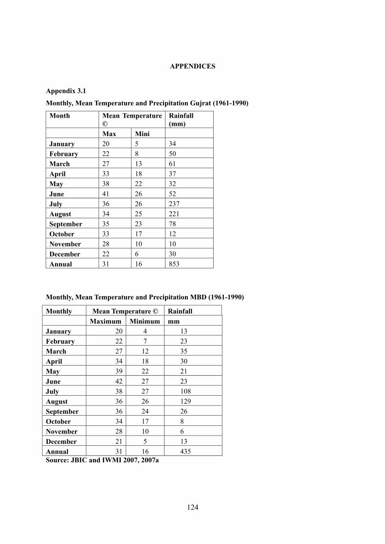
124
APPENDICES
Appendix 3.1
Monthly, Mean Temperature and Precipitation Gujrat (1961-1990)
Month Mean Temperature
©
Rainfall
(mm)
Max Mini
January 20 5 34
February 22 8 50
March 27 13 61
April 33 18 37
May 38 22 32
June 41 26 52
July 36 26 237
August 34 25 221
September 35 23 78
October 33 17 12
November 28 10 10
December 22 6 30
Annual 31 16 853
Monthly, Mean Temperature and Precipitation MBD (1961-1990)
Monthly Mean Temperature © Rainfall
Maximum Minimum mm
January 20 4 13
February 22 7 23
March 27 12 35
April 34 18 30
May 39 22 21
June 42 27 23
July 38 27 108
August 36 26 129
September 36 24 26
October 34 17 8
November 28 10 6
December 21 5 13
Annual 31 16 435
Source: JBIC and IWMI 2007, 2007a
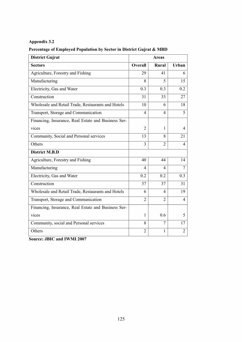
125
Appendix 3.2
Percentage of Employed Population by Sector in District Gujrat & MBD
District Gujrat Areas
Sectors Overall Rural Urban
Agriculture, Forestry and Fishing 29 41 6
Manufacturing 8 5 15
Electricity, Gas and Water 0.3 0.3 0.2
Construction 31 33 27
Wholesale and Retail Trade, Restaurants and Hotels 10 6 18
Transport, Storage and Communication 4 4 5
Financing, Insurance, Real Estate and Business Ser-
vices 2 1 4
Community, Social and Personal services 13 8 21
Others 3 2 4
District M.B.D
Agriculture, Forestry and Fishing 40 44 14
Manufacturing 4 4 7
Electricity, Gas and Water 0.2 0.2 0.3
Construction 37 37 31
Wholesale and Retail Trade, Restaurants and Hotels 6 4 19
Transport, Storage and Communication 2 2 4
Financing, Insurance, Real Estate and Business Ser-
vices 1 0.6 5
Community, social and Personal services 8 7 17
Others 2 1 2
Source: JBIC and IWMI 2007
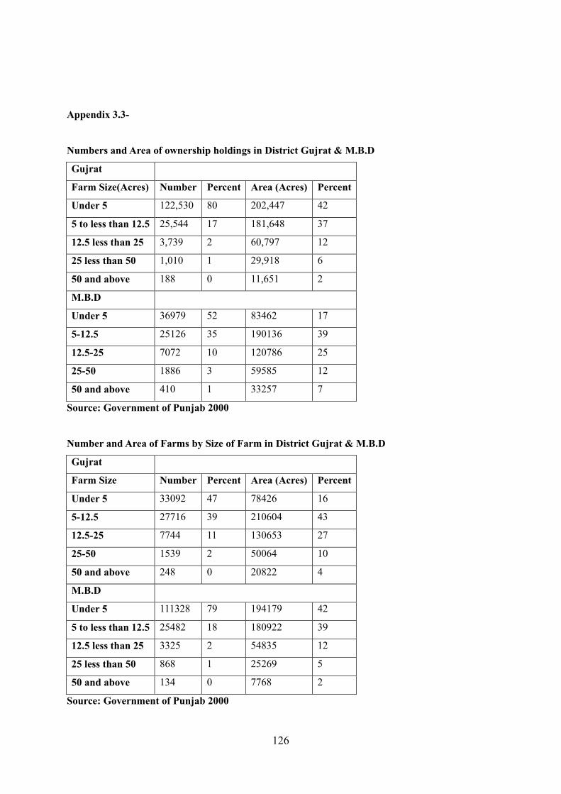
126
Appendix 3.3-
Numbers and Area of ownership holdings in District Gujrat & M.B.D
Gujrat
Farm Size(Acres) Number Percent Area (Acres) Percent
Under 5 122,530 80 202,447 42
5 to less than 12.5 25,544 17 181,648 37
12.5 less than 25 3,739 2 60,797 12
25 less than 50 1,010 1 29,918 6
50 and above 188 0 11,651 2
M.B.D
Under 5 36979 52 83462 17
5-12.5 25126 35 190136 39
12.5-25 7072 10 120786 25
25-50 1886 3 59585 12
50 and above 410 1 33257 7
Source: Government of Punjab 2000
Number and Area of Farms by Size of Farm in District Gujrat & M.B.D
Gujrat
Farm Size Number Percent Area (Acres) Percent
Under 5 33092 47 78426 16
5-12.5 27716 39 210604 43
12.5-25 7744 11 130653 27
25-50 1539 2 50064 10
50 and above 248 0 20822 4
M.B.D
Under 5 111328 79 194179 42
5 to less than 12.5 25482 18 180922 39
12.5 less than 25 3325 2 54835 12
25 less than 50 868 1 25269 5
50 and above 134 0 7768 2
Source: Government of Punjab 2000
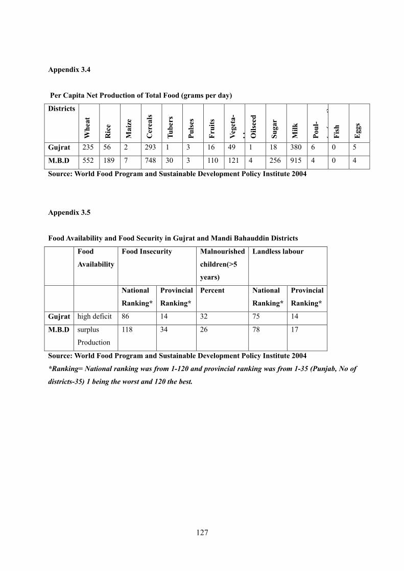
127
Appendix 3.4
Per Capita Net Production of Total Food (grams per day)
Districts
Wheat
Rice
Maize
Cereals
Tubers
Pulses
Fruits
Vegeta-
ble
Oilseed
Sugar
Milk
Poul-
try(m
eat)
Fish
Eggs
Gujrat 235 56 2 293 1 3 16 49 1 18 380 6 0 5
M.B.D 552 189 7 748 30 3 110 121 4 256 915 4 0 4
Source: World Food Program and Sustainable Development Policy Institute 2004
Appendix 3.5
Food Availability and Food Security in Gujrat and Mandi Bahauddin Districts
Food
Availability
Food Insecurity Malnourished
children(>5
years)
Landless labour
National
Ranking*
Provincial
Ranking*
Percent National
Ranking*
Provincial
Ranking*
Gujrat high deficit 86 14 32 75 14
M.B.D surplus
Production
118 34 26 78 17
Source: World Food Program and Sustainable Development Policy Institute 2004
*Ranking= National ranking was from 1-120 and provincial ranking was from 1-35 (Punjab, No of
districts-35) 1 being the worst and 120 the best.
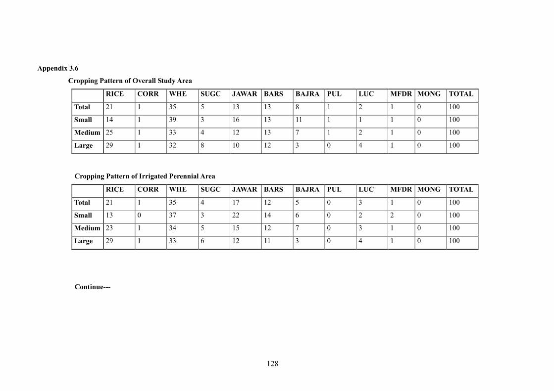
128
Appendix 3.6
Cropping Pattern of Overall Study Area
RICE CORR WHE SUGC JAWAR BARS BAJRA PUL LUC MFDR MONG TOTAL
Total 21 1 35 5 13 13 8 1 2 1 0 100
Small 14 1 39 3 16 13 11 1 1 1 0 100
Medium 25 1 33 4 12 13 7 1 2 1 0 100
Large 29 1 32 8 10 12 3 0 4 1 0 100
Cropping Pattern of Irrigated Perennial Area
RICE CORR WHE SUGC JAWAR BARS BAJRA PUL LUC MFDR MONG TOTAL
Total 21 1 35 4 17 12 5 0 3 1 0 100
Small 13 0 37 3 22 14 6 0 2 2 0 100
Medium 23 1 34 5 15 12 7 0 3 1 0 100
Large 29 1 33 6 12 11 3 0 4 1 0 100
Continue---
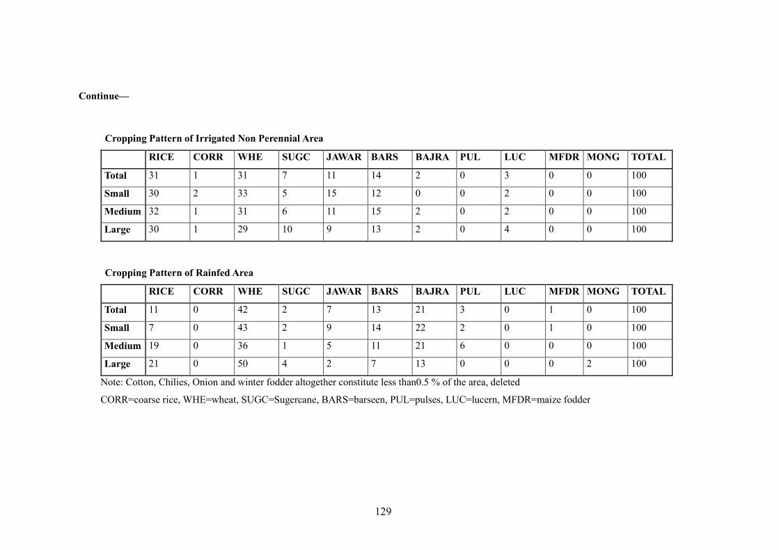
129
Continue—
Cropping Pattern of Irrigated Non Perennial Area
RICE CORR WHE SUGC JAWAR BARS BAJRA PUL LUC MFDR MONG TOTAL
Total 31 1 31 7 11 14 2 0 3 0 0 100
Small 30 2 33 5 15 12 0 0 2 0 0 100
Medium 32 1 31 6 11 15 2 0 2 0 0 100
Large 30 1 29 10 9 13 2 0 4 0 0 100
Cropping Pattern of Rainfed Area
RICE CORR WHE SUGC JAWAR BARS BAJRA PUL LUC MFDR MONG TOTAL
Total 11 0 42 2 7 13 21 3 0 1 0 100
Small 7 0 43 2 9 14 22 2 0 1 0 100
Medium 19 0 36 1 5 11 21 6 0 0 0 100
Large 21 0 50 4 2 7 13 0 0 0 2 100
Note: Cotton, Chilies, Onion and winter fodder altogether constitute less than0.5 % of the area, deleted
CORR=coarse rice, WHE=wheat, SUGC=Sugercane, BARS=barseen, PUL=pulses, LUC=lucern, MFDR=maize fodder
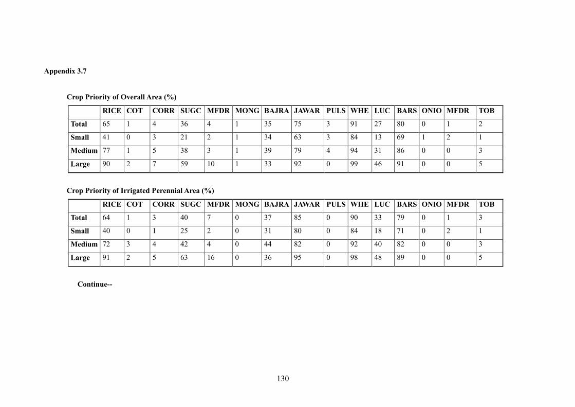
130
Appendix 3.7
Crop Priority of Overall Area (%)
RICE COT CORR SUGC MFDR MONG BAJRA JAWAR PULS WHE LUC BARS ONIO MFDR TOB
Total 65 1 4 36 4 1 35 75 3 91 27 80 0 1 2
Small 41 0 3 21 2 1 34 63 3 84 13 69 1 2 1
Medium 77 1 5 38 3 1 39 79 4 94 31 86 0 0 3
Large 90 2 7 59 10 1 33 92 0 99 46 91 0 0 5
Crop Priority of Irrigated Perennial Area (%)
RICE COT CORR SUGC MFDR MONG BAJRA JAWAR PULS WHE LUC BARS ONIO MFDR TOB
Total 64 1 3 40 7 0 37 85 0 90 33 79 0 1 3
Small 40 0 1 25 2 0 31 80 0 84 18 71 0 2 1
Medium 72 3 4 42 4 0 44 82 0 92 40 82 0 0 3
Large 91 2 5 63 16 0 36 95 0 98 48 89 0 0 5
Continue--
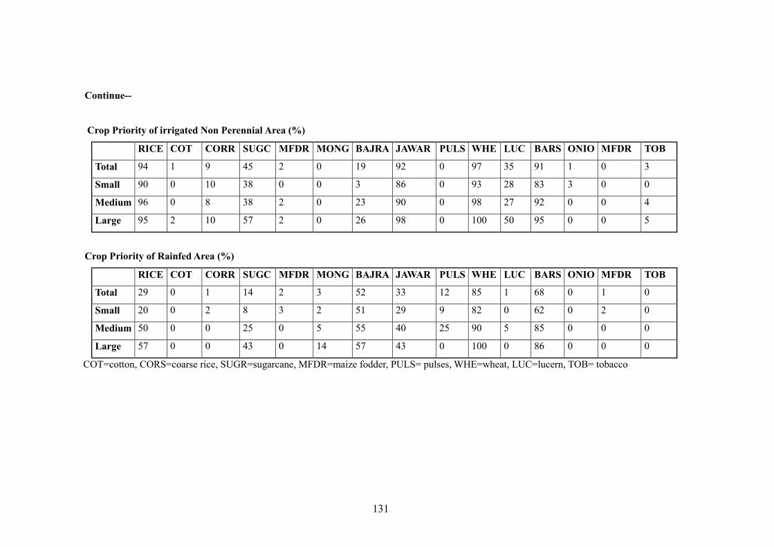
131
Continue--
Crop Priority of irrigated Non Perennial Area (%)
RICE COT CORR SUGC MFDR MONG BAJRA JAWAR PULS WHE LUC BARS ONIO MFDR TOB
Total 94 1 9 45 2 0 19 92 0 97 35 91 1 0 3
Small 90 0 10 38 0 0 3 86 0 93 28 83 3 0 0
Medium 96 0 8 38 2 0 23 90 0 98 27 92 0 0 4
Large 95 2 10 57 2 0 26 98 0 100 50 95 0 0 5
Crop Priority of Rainfed Area (%)
RICE COT CORR SUGC MFDR MONG BAJRA JAWAR PULS WHE LUC BARS ONIO MFDR TOB
Total 29 0 1 14 2 3 52 33 12 85 1 68 0 1 0
Small 20 0 2 8 3 2 51 29 9 82 0 62 0 2 0
Medium 50 0 0 25 0 5 55 40 25 90 5 85 0 0 0
Large 57 0 0 43 0 14 57 43 0 100 0 86 0 0 0
COT=cotton, CORS=coarse rice, SUGR=sugarcane, MFDR=maize fodder, PULS= pulses, WHE=wheat, LUC=lucern, TOB= tobacco
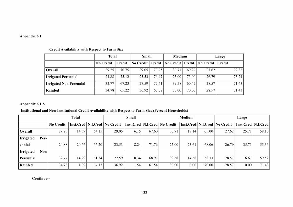
132
Appendix 6.1
Credit Availability with Respect to Farm Size
Total Small Medium Large
No Credit Credit No Credit Credit No Credit Credit No Credit Credit
Overall 29.25 70.75 29.05 70.95 30.71 69.29 27.62 72.38
Irrigated Perennial 24.88 75.12 23.53 76.47 25.00 75.00 26.79 73.21
Irrigated Non Perennial 32.77 67.23 27.59 72.41 39.58 60.42 28.57 71.43
Rainfed 34.78 65.22 36.92 63.08 30.00 70.00 28.57 71.43
Appendix 6.1 A
Institutional and Non-Institutional Credit Availability with Respect to Farm Size (Percent Households)
Total Small Medium Large
No Credit Inst.Cred N.I.Cred No Credit Inst.Cred N.I.Cred No Credit Inst.Cred N.I.Cred No Credit Inst.Cred N.I.Cred
Overall 29.25 14.39 64.15 29.05 6.15 67.60 30.71 17.14 65.00 27.62 25.71 58.10
Irrigated Per-
ennial 24.88 20.66 66.20 23.53 8.24 71.76 25.00 23.61 68.06 26.79 35.71 55.36
Irrigated Non
Perennial 32.77 14.29 61.34 27.59 10.34 68.97 39.58 14.58 58.33 28.57 16.67 59.52
Rainfed 34.78 1.09 64.13 36.92 1.54 61.54 30.00 0.00 70.00 28.57 0.00 71.43
Continue--
133
Continue--
N.I. Credit = Non-institutional credit
Inst.Credit = Institutional credit
No Credit: Neither institutional nor non-institutional credit was taken by households
Institutional Credit: Credit taken from banks and cooperatives
Non-Institutional Credit: Credit taken from friends, relatives, non-relatives, traders and dealers etc.