Embed Size (px)
Citation preview
Loyola University Chicago Loyola University Chicago
Loyola eCommons Loyola eCommons
Master's Theses Theses and Dissertations
2010
Resource Composition and Macroinvertebrate Resource Resource Composition and Macroinvertebrate Resource
Consumption in the Colorado River Below Glen Canyon Dam Consumption in the Colorado River Below Glen Canyon Dam
Holly Ann Alfreda Wellard Kelly Loyola University Chicago
Follow this and additional works at: https://ecommons.luc.edu/luc_theses
Part of the Ecology and Evolutionary Biology Commons
Recommended Citation Recommended Citation Wellard Kelly, Holly Ann Alfreda, "Resource Composition and Macroinvertebrate Resource Consumption in the Colorado River Below Glen Canyon Dam" (2010). Master's Theses. 555. https://ecommons.luc.edu/luc_theses/555
This Thesis is brought to you for free and open access by the Theses and Dissertations at Loyola eCommons. It has been accepted for inclusion in Master's Theses by an authorized administrator of Loyola eCommons. For more information, please contact [email protected].
This work is licensed under a Creative Commons Attribution-Noncommercial-No Derivative Works 3.0 License. Copyright © 2010 Holly Ann Alfreda Wellard Kelly
LOYOLA UNIVERSITY CHICAGO
RESOURCE COMPOSITION AND
MACROINVERTEBRATE RESOURCE CONSUMPTION IN THE
COLORADO RIVER BELOW GLEN CANYON DAM
A THESIS SUBMITTED TO
THE FACULTY OF THE GRADUATE SCHOOL
IN CANDIDACY FOR THE DEGREE OF
MASTER OF SCIENCE
PROGRAM IN BIOLOGY
BY
HOLLY ANN WELLARD KELLY
CHICAGO, IL
AUGUST 2010

Copyright by Holly A. Wellard Kelly, 2010 All rights reserved
iii
ACKNOWLEDGEMENTS
I have many people to thank for their help throughout graduate school. First, I
must thank my family for their endless supply of encouragement, for always believing in
me, and for instilling in me a love of the outdoors. I would like to acknowledge my
mother and Sam for their help designing and sewing sampling nets. I owe a special
thanks to my husband Sam for his love and support during the three years we spent apart.
Finally, I thank all my friends, particularly my oldest friend Lindsey Good, for providing
stress relieving activities, advice, and support throughout graduate school and life.
Thanks to everyone in the Rosi-Marshall Lab. In particular, I acknowledge
Antoine Aubeneau for helping me write macros and learn new computer programs, and
Paul Hoppe and Sarah Zahn, for their help with laboratory and field work. I owe great
thanks to everyone on the Colorado River Ecosystems Studies Team, particularly the
technicians, Amber Adams, Kate Behn, and Adam Copp, for preparing everything for
river trips and collecting my samples when I was not there. I also thank Amber Ulseth,
for her help in the field and for sharing her tent during inclement weather. Special thanks
to the many boatmen, whose whitewater rafting knowledge and expertise made sampling
possible, and whose great personalities made every river trip the time of my life.
I would like to especially thank my committee members and the principal
investigators on my project: Dr. Martin Berg, Dr. Chris Peterson, Dr. Ted Kennedy, Dr.
Colden Baxter, Dr. Bob Hall, and Dr. Wyatt Cross, for teaching me about stream
iv
ecology, aquatic entomology, algal ecology, and statistics, and helping me to think
critically about science and my project. I give my greatest thanks to my adviser, Dr.
Emma Rosi-Marshall for her endless stream of ideas and guidance through this process. I
could not have finished without her support. Thank you for teaching me and making
graduate school so much fun.
Finally, I thank C. Donato, J. Kampman, S. Khan, D. Kincaid, D. Lee, S. Lee, J.
Nunnally, K. Pfeifer, A. Salma, Y. Sayeed, J. Stanton, K. Vallis, T. White, M. Yard, for
assistance with field and laboratory work, data analysis and editing. This work was
supported by a grant from the United States Geological Survey, Grand Canyon
Monitoring and Research Center.

This work is dedicated to my mother and father, Judd and Mary Ann Wellard, my brother and sister, Scott and Ann Wellard, and my husband, Sam Kelly, for their unconditional
love and support throughout my life and the course of this thesis.
vi
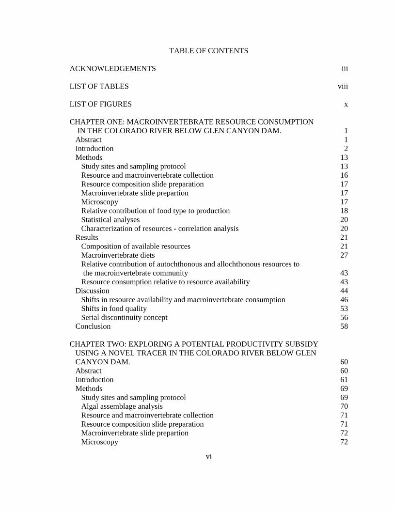
TABLE OF CONTENTS
ACKNOWLEDGEMENTS iii LIST OF TABLES viii LIST OF FIGURES x CHAPTER ONE: MACROINVERTEBRATE RESOURCE CONSUMPTION
IN THE COLORADO RIVER BELOW GLEN CANYON DAM. 1 Abstract 1 Introduction 2 Methods 13
Study sites and sampling protocol 13 Resource and macroinvertebrate collection 16 Resource composition slide preparation 17 Macroinvertebrate slide prepartion 17 Microscopy 17 Relative contribution of food type to production 18 Statistical analyses 20 Characterization of resources - correlation analysis 20
Results 21 Composition of available resources 21 Macroinvertebrate diets 27 Relative contribution of autochthonous and allochthonous resources to the macroinvertebrate community 43 Resource consumption relative to resource availability 43
Discussion 44 Shifts in resource availability and macroinvertebrate consumption 46 Shifts in food quality 53 Serial discontinuity concept 56
Conclusion 58 CHAPTER TWO: EXPLORING A POTENTIAL PRODUCTIVITY SUBSIDY
USING A NOVEL TRACER IN THE COLORADO RIVER BELOW GLEN CANYON DAM. 60 Abstract 60 Introduction 61 Methods 69
Study sites and sampling protocol 69 Algal assemblage analysis 70 Resource and macroinvertebrate collection 71 Resource composition slide preparation 71 Macroinvertebrate slide prepartion 72 Microscopy 72
vii
Algal movement and survival 73 Algal transport distance and deposition velocity 73 Algal species as indicators of tailwater production 74
Results 78 Longitudinal transport and survival of Fragilaria crotonensis 79 Algal transport distance and deposition velocity 80 Dominant taxa as indicators 81 Rare taxa 87 Final list and consumption by macroinvertebrates 88
Discussion 92 Summary of results 92 Algal downstream transport and survival 93 Macroinvertebrate consumption of indicators 98 DCA, area plots and rare taxa analysis for indicator identification 99 Indicator presence and preferences 100 Utility of the method/usefulness of algae as indicators/tracers 101
Conclusion 103 APPENDIX A: ONE-WAY ANOVA TABLES 105 APPENDIX B: ALGAL COMMUNITY COMPOSITION TABLES 134 REFERENCES 153 VITA 169
viii
LIST OF TABLES
Table 1. Site, season, and month of sample collection, and associated light condition, water condition, average monthly sediment concentration (mg/L), and prediction describing which resources (autochthonous or allochthonous) will be predominately consumed by macroinvertebrates. 12
Table 2. Mean site characteristics. 16 Table 3. Mean proportion and standard error (SE) of particle types comprising
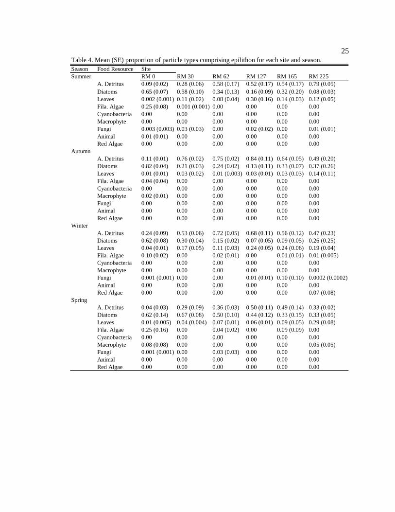
suspended organic seston for each site and season. 23 Table 4. Mean proportion and standard error (SE) of particle types comprising
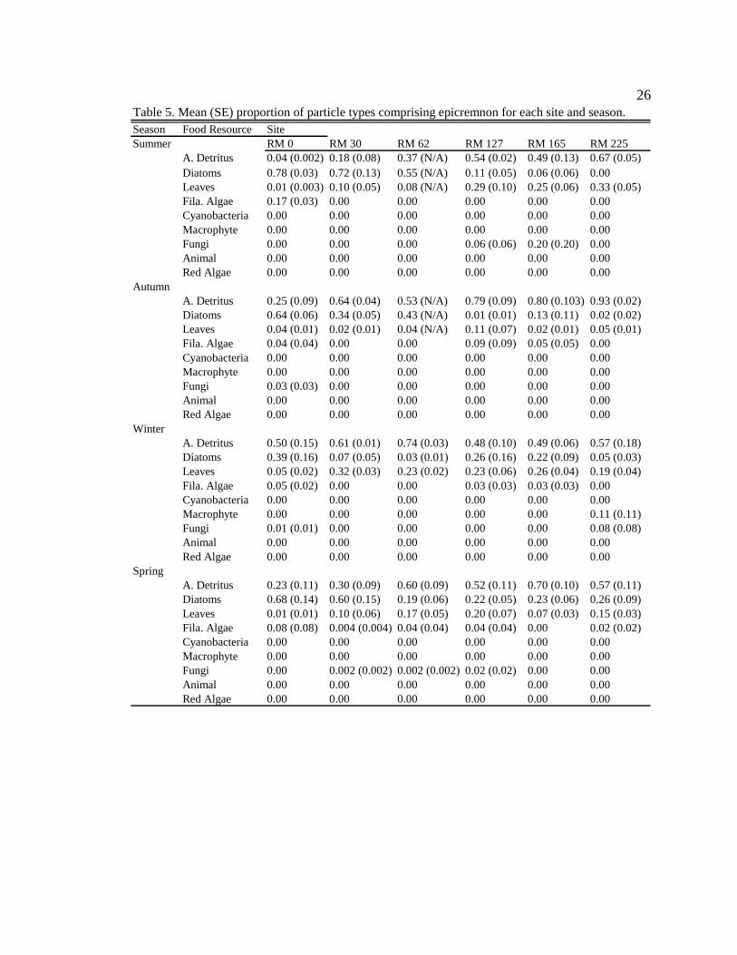
epilithon for each site and season. 25 Table 5. Mean proportion and standard error (SE) of particle types comprising
epicremnon for each site and season. 26 Table 6. Mean proportion and standard error (SE) of consumption by Simulium
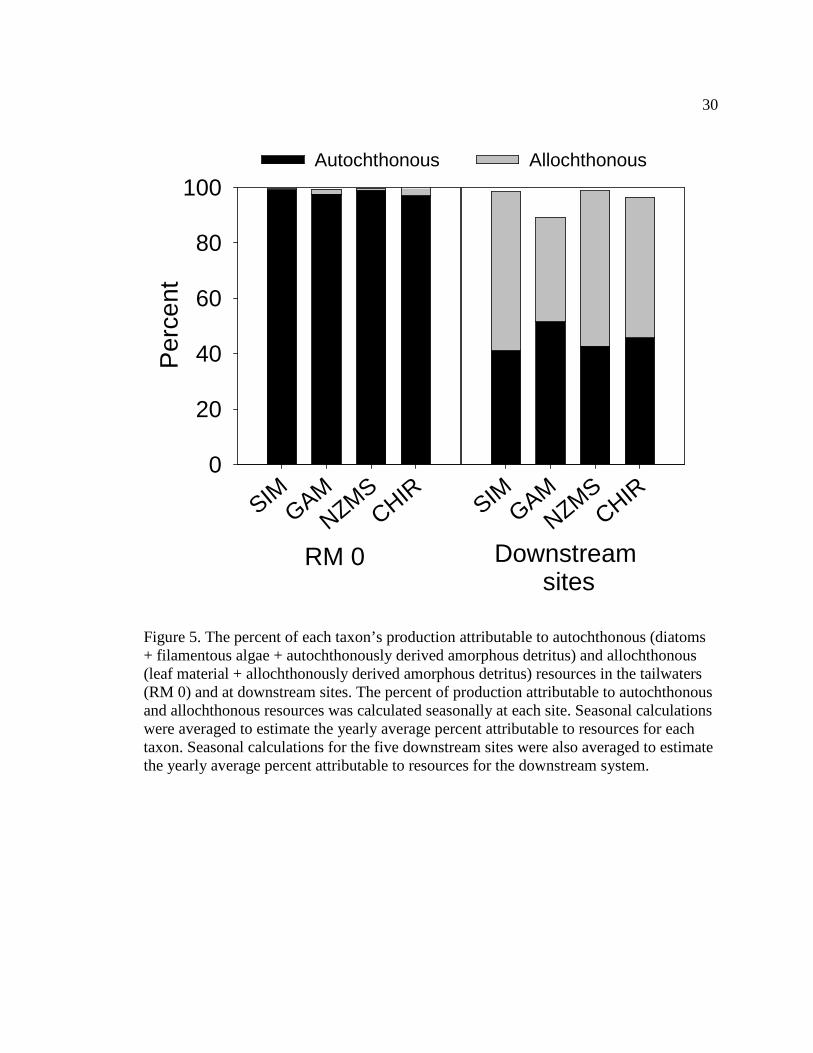
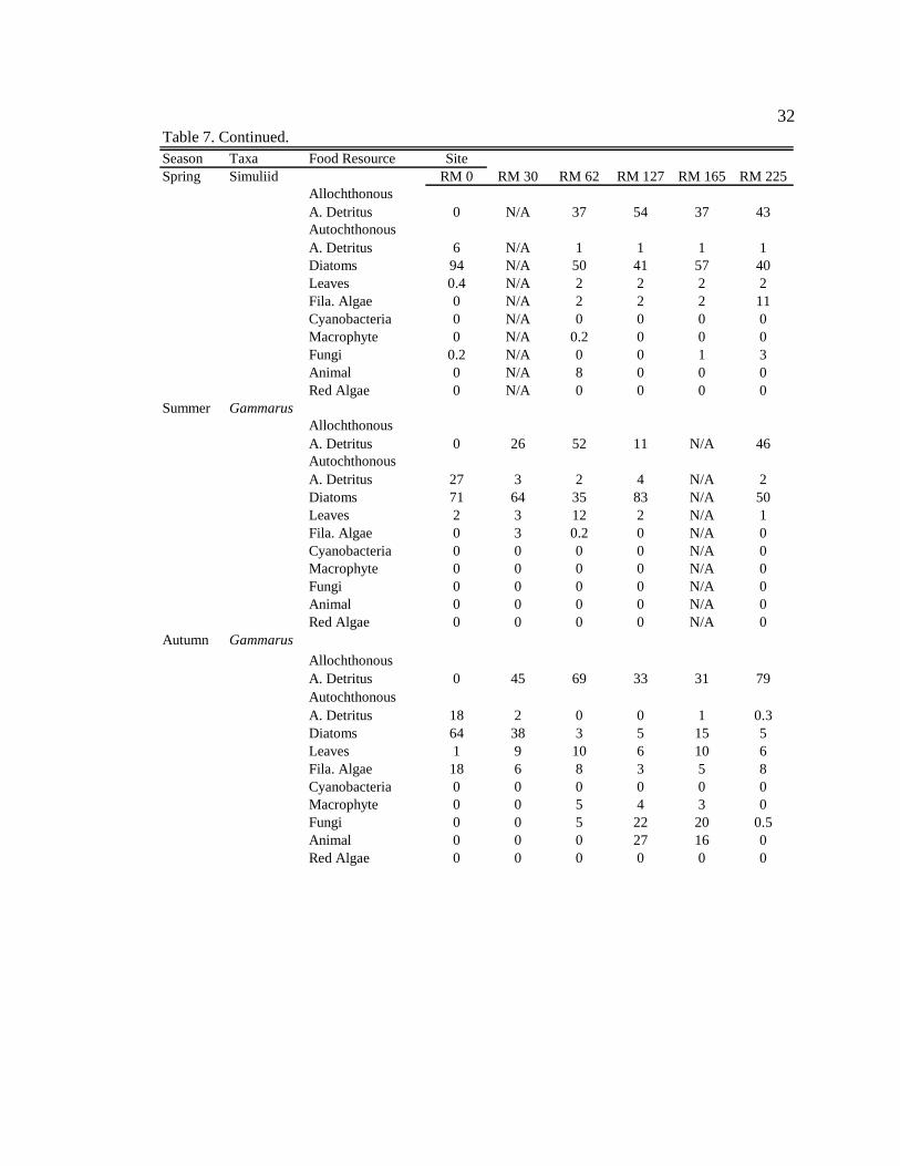
arcticum for each site and season. 29 Table 7. Production attributed to food type (%). Calculation: Food type in gut (%)
×Assimilation efficiency (AE) x Net production efficiency (NPE)/ Σ (G (a+b+c…n) × AE ×NPE). 31
Table 8. Mean proportion and standard error (SE) of consumption by Gammarus
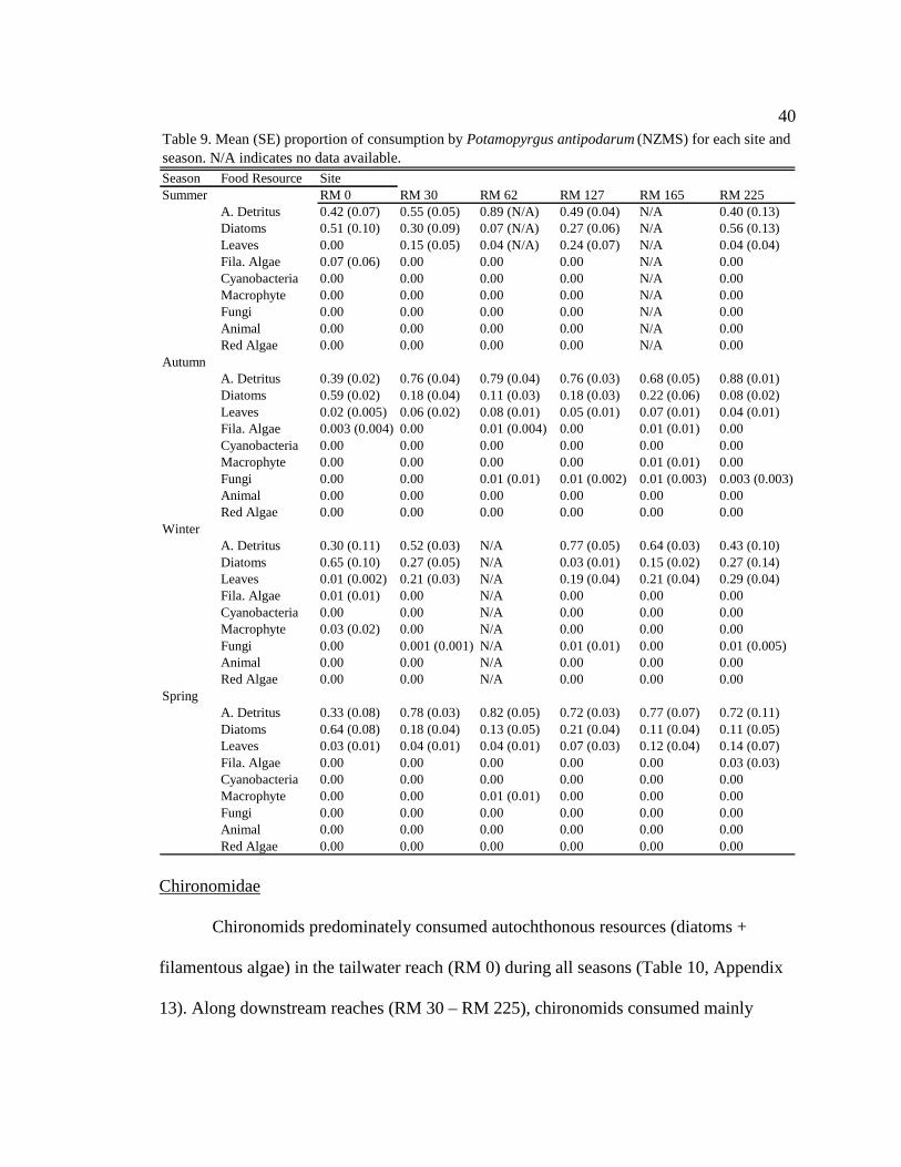
lacustris for each site and season. 38 Table 9. Mean proportion and standard error (SE) of consumption by
Potamopyrgus antipodarum (NZMS) for each site and season. 40 Table 10. Mean proportion and standard error (SE) of consumption by
Chironomidae for each site and season. 42 Table11. Correlation results examining the relationship between the percent
composition of a particle type in the seston or epilithon/rock faces and the percent consumption of the particle type by each taxon. r = Pearson product-moment correlation coefficient and associated p-value. 44

ix
Table 12. Final list of tailwater and downstream algal indicators, the habitats they are indicators of, and the sites where they are consumed by downstream macroinvertebrates. Numbers in parentheses represent the percent of the community the indicator represented in the diet. 89
x
LIST OF FIGURES Figure 1. Effects of the dam and tributary inputs on organic matter budgets and
potential influence on macroinvertebrate food web. 11 Figure 2. Map of the Colorado River in Grand Canyon showing the location of the
six sites sampled. 15 Figure 3. The proportion of particles types comprising suspended organic seston at
six sites downstream of dam during A) summer 2006; B) autumn 2006; C) winter 2007; and D) spring 2007. 22
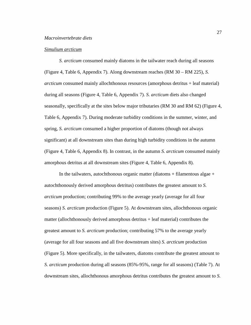
Figure 4. The proportion of particle types consumed seasonally by Simulium
arcticum at six sites downstream of dam during A) summer 2006; B) autumn 2006; C) winter 2007; and D) spring 2007. 28
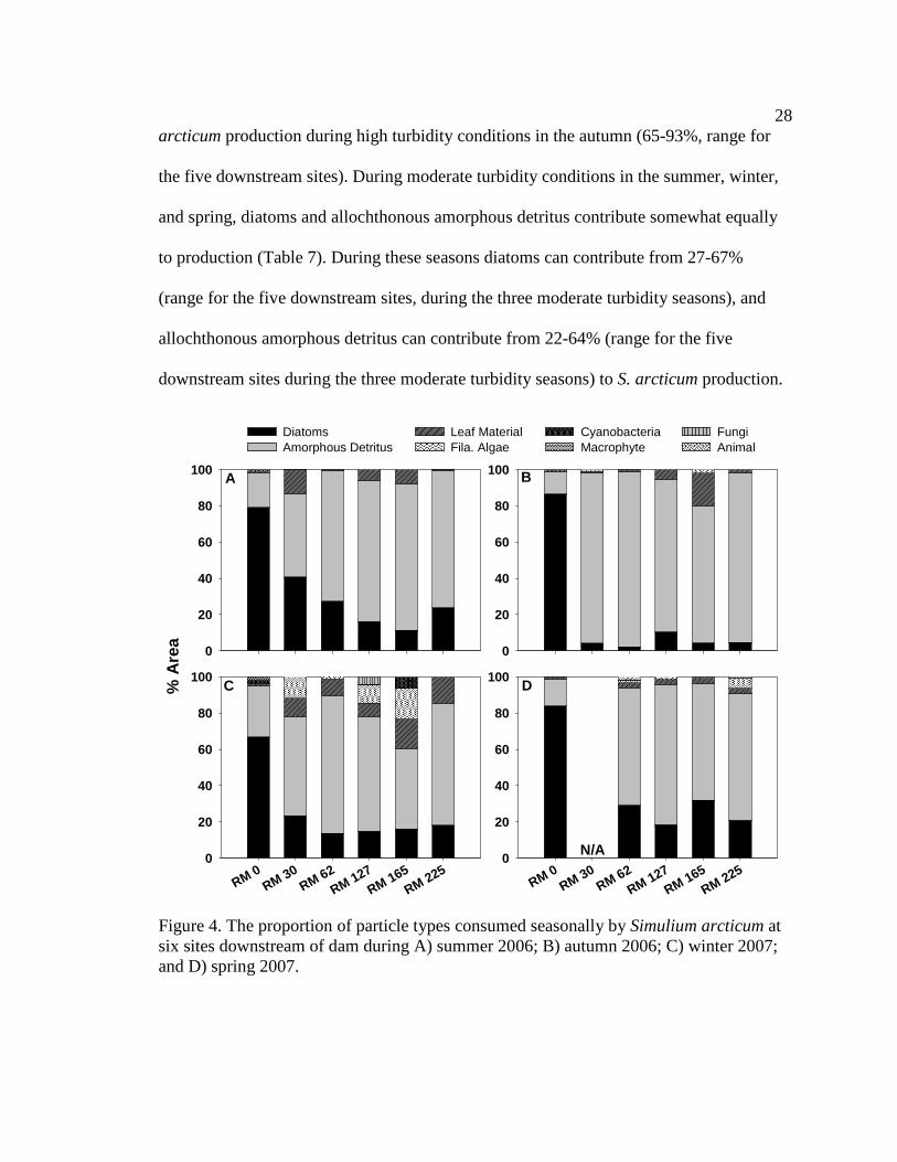
Figure 5. The percent of each taxon’s production attributable to autochthonous
(diatoms + filamentous algae + autochthonously derived amorphous detritus) and allochthonous (leaf material + allochthonously derived amorphous detritus) resources in the tailwaters (RM 0) and at downstream sites. The percent of production attributable to autochthonous and allochthonous resources was calculated seasonally at each site. Seasonal calculations were averaged to estimate the yearly average percent attributable to resources for each taxon. Seasonal calculations for the five downstream sites were also averaged to estimate the yearly average percent attributable to resources for the downstream system. 30
Figure 6. Correlation analysis of the average percent particle type (diatoms or
amorphous detritus) comprising an available food resource (seston or epilithon) versus the average percent of the diet the particle comprises, at each site, during each season. A, B) Seston vs. S. arcticum; C, D) epilithon vs. G. lacustris; E, F) epilithon vs. NZMS; G,H) epilithon vs. chironomids. Pearson product-moment correlation coefficients (r) and associated p-values are given. Line represents the line of equity (one-to-one relationship). Points above the line demonstrate that the percent of the particle type consumed by the macroinvertebrate is greater than the percent composition of the particle type in the food resource. Points below the line demonstrate that the percent of the particle type consumed
xi
by the macroinvertebrate is less than the percent composition of the particle type in the food resource. 45
Figure 7. Effects of the dam and tributary inputs on algal communities. 67 Figure 8. Potential algal sources for macroinvertebrates at downstream sites. 68 Figure 9. Flow chart used to classify tailwater and downstream indicator species. 77 Figure 10. Area plot of dominant taxa (mean is ≥ 3% of the assemblage) in seston at
six sites downstream of the dam. See Appendix B: Appendix 15 for algal species list and corresponding species code. 82
Figure 11. Area plot of dominant taxa (mean is ≥ 3% of the assemblage) in
epilithon at six sites downstream of the dam. See Appendix B: Appendix 15 for algal species list and corresponding species code. 84
Figure 12. Area plot of dominant taxa (mean is ≥ 3% of the assemblage) in
epicremnon at six sites downstream of the dam. See Appendix B: Appendix 15 for algal species list and corresponding species code. 86
Figure 13. Mean number and standard deviation (SD) of alive and dead Fragilaria
crotonensis Kitton cells per milliliter of filtered suspended organic matter (seston) at six sites downstream of the dam. Seston samples collected at each site were sampling different pulses of water released from the dam (i.e. I did not follow and sample the same water at each site in the canyon). 79
Figure 14. Mean percent and standard deviation (SD) of F. crotonensis Kitton in the
seston algal assemblage, and S. arcticum diet algal assemblage, at six sites downstream of the dam. And the mean percent F. crotonensis comprises of total particles in S. arcticum diets at six sites downstream of the dam. 80
Figure 15. A) DCA ordination of mean (SD) sample scores for seston in January
2007 at six sites downstream of dam. Eigenvalues for axis 1 = 0.362; for axis 2 = 0078. B) Corresponding species scores (see Appendix B: Appendix 15 for abbreviations). 82
Figure 16. A) DCA ordination of mean (SD) sample scores for epilithon in January
2007 at six sites downstream of dam. Eigenvalues for axis 1 = 0.632; for axis 2 = 0.170. B) Corresponding species scores (see Appendix B: Appendix 15 for abbreviations). 84
xii
Figure 17. A) DCA ordination of mean (SD) sample scores for epicremnon in January 2007 at six sites downstream of dam. Eigenvalues for axis 1 = 0.461; for axis 2 = 0.272. B) Corresponding species scores (see Appendix B: Appendix 15 for abbreviations). 86
Figure 18. Percent of S. arcticum production attributable to tailwater indicator
diatoms, and all other non-indicator diatoms, at six sites downstream of the dam. 91
Figure 19. Percent of G. lacustris production attributable to tailwater indicator
diatoms, and all other non-indicator diatoms, at six sites downstream of the dam. 92
1
CHAPTER ONE
MACROINVERTEBRATE RESOURCE CONSUMPTION IN THE
COLORADO RIVER BELOW GLEN CANYON DAM
Abstract
Physical and biological changes to rivers induced by large dams can significantly
impact downstream communities, decreasing the biotic integrity of these rivers. The
completion of Glen Canyon Dam on the Colorado River in 1963 has altered the
downstream ecosystem and contributed to the decline of native fish populations in the
river. Macroinvertebrates are an important food resource for fish and determining the
relative importance of basal resources to macroinvertebrate production will help guide
the development of a long-term lower trophic level monitoring program. Because
autochthonous production is high in the tailwater reach and tributary allochthonous
carbon inputs are substantial at downstream sites, I predict that macroinvertebrate diets
will reflect longitudinal changes in resource availability. I also predict that seasonal
changes in resource availability due to monsoon tributary flooding in the autumn and
lower light availability in the winter, will amplify the longitudinal change in resource use
by macroinvertebrates. I examined the diets of the common macroinvertebrates
(Simulium arcticum, Gammarus lacustris, Potamopyrgus antipodarum, and chironomids)
at six sites below Glen Canyon Dam during all seasons. Macroinvertebrate diet
composition was compared to the composition of the epilithon (rock faces), epicremnon
2
(cliff faces) communities, and the suspended organic seston. The relative contribution of
autochthonous and allochthonous resources to macroinvertebrate production was
calculated at all six sites. In general, macroinvertebrate diets tracked downstream changes
in resource availability in the river, and autochthonous resources were consumed in
greater proportions in the tailwaters while more allochthonous resources were consumed
downstream. Also autochthonous resources contributed more to macroinvertebrate
production in the tailwaters and allochthonous resources contributed more downstream.
The extent of diet shifts depended on consumer identity and season. Diets of S. arcticum
differed among all seasons, whereas the diets of other taxa only differed during the
autumn and winter. Allochthonous resources were most important for all consumers
during the monsoon season (July-September), when tributaries can contribute significant
amounts of organic matter to the mainstem. These data demonstrate that both
autochthonous and allochthonous resources support macroinvertebrate production in the
Grand Canyon; however, the contribution of allochthonous resources to
macroinvertebrate production increases at downstream sites.
Introduction
Large dams alter the physical habitat, temperature and flow regimes of rivers and
have contributed significantly to the degradation of freshwater ecosystems worldwide
(Baxter 1977, Ward and Stanford 1979, Petts 1984, Nilsson and Berggren 2000). The
physical changes induced by dams can significantly affect riverine biodiversity and food
webs (Power et al. 1996), often reducing biodiversity of algae, macroinvertebrate and fish
communities (Allan and Flecker 1993). Dam-induced physical and chemical changes in

3
rivers are most drastic in the tailwaters where non-native taxa often thrive (Stanford et al.
1996). Tributaries downstream of dams ameliorate the effects of dams on rivers physical
and chemical properties (Ward and Stanford 1983); therefore, communities that are
downstream of tributaries may differ from tailwater communities (Takao et al. 2008).
The Colorado River has been physically and biologically altered due to
construction of Glen Canyon Dam (Blinn and Cole 1991). Historically, the river had high
seasonal variability in temperature and discharge (Topping et al. 2003), was at times
extremely sediment-laden (Wright et al. 2005), and sustained a highly endemic native
fish community (Gloss and Coggins 2005) and diverse macroinvertebrate populations
(Musser 1959, Edmunds 1959, Haden et al. 2003, Hofnecht 1981, Oberlin et al. 1999).
Dam-associated alterations in the physical template and intentional and unintentional
introductions of non-native fishes and macroinvertebrates have significantly altered food
web structure, and four of the eight species of fish native to Grand Canyon have been
locally extirpated while one of the remaining species, humpback chub (Gila cypha), is
federally endangered (Minckley et. al 2003).
A variety of factors may limit populations of native fish in Grand Canyon
including habitat availability, competition with and predation by non-native species, and
food resource availability (Gloss and Coggins 2005). Macroinvertebrates are an
important food resource for fish throughout the lower Colorado River basin (Childs et al.
1998, Zahn et al. unpublished data) and declines in native fish populations may be due to
food limitation (i.e. low macroinvertebrate production) at the base of the food web. To
successfully manage this highly modified ecosystem to support macroinvertebrate and
4
native fish populations, it is crucial to understand the food resources (allochthonous vs.
autochthonous) supporting the base of the food web and how energy flows through the
food web. An important first step in elucidating energy flow through the entire food web
is to assess food resources consumed by macroinvertebrates.
Limited literature documents the pre-impoundment macroinvertebrate
communities of the Colorado River in Grand Canyon (Blinn and Cole 1991). Musser
(1959) surveyed macroinvertebrate species from the Colorado River in Glen Canyon and
reported 91 species from the following eight orders: Ephemeroptera, Odonata,
Hemiptera, Megaloptera, Trichoptera, Lepidoptera, Coleoptera, and Diptera. Although
collection methods are not clearly reported, the majority of species were collected from
tributaries, and only 247 of the 2,315 individuals collected were from the mainstem
(Musser 1959). Edmunds (1959) reports six families and eight genera of mayflies in the
area of Glen Canyon Dam before impoundment. The macroinvertebrate fauna of Cataract
Canyon, an unregulated reach of the Colorado River immediately upriver of Lake Powell,
is likely analogous to pre-impoundment Colorado River conditions because this reach is
geomorphically similar to Grand Canyon and has suspended sediment concentrations and
discharge regimes that closely match pre-impoundment conditions (Stanford and Ward
1986, Haden et al. 2003). Forty-nine macroinvertebrate taxa were identified in this reach,
with most taxa from the orders, Ephemeroptera, Plecoptera, Trichoptera, and Diptera
(Haden et al. 2003).
Post-impoundment studies of macroinvertebrate communities in tributaries of the
Colorado River through Grand Canyon may also provide useful indicators of the
5
mainstem pre-impoundment macroinvertebrate community (Hofnecht 1981, Oberlin et al.
1999). Between 23-52 macroinvertebrate families have been reported in tributaries
throughout the Grand Canyon (Hofnecht 1981, Oberlin et al. 1999), with representatives
of the order Trichoptera the most diverse, comprising nine families and twelve genera
(Oberlin et al. 1999). In addition, macroinvertebrates from six orders: Ephemeroptera,
Lepidoptera, Diptera, Megaloptera, Coleoptera, and Plecoptera, are present in tributaries
(Oberlin et al. 1999).
Numerous pre-impoundment studies of the Green River, Utah, approximately 180
miles upstream from Glen Canyon Dam, may provide additional insight into the pre-dam
Colorado River Grand Canyon macroinvertebrate community assemblage (Vinson 2001).
Prior to the completion of the Flaming Gorge Dam in 1962, the Green River supported a
diverse macroinvertebrate community (Pearson et al. 1968, Vinson 2001) including
species within the orders: Nematoda, Oligochaeta, Hirudinea, Amphipoda, Hydracarina,
Plecoptera, Ephemeroptera, Odonata, Hemiptera, Megaloptera, Trichoptera, Lepidoptera,
Coleoptera, Diptera, and Gastropoda. Most of the taxa reported above were extirpated
after the completion of the Flaming Gorge Dam (Vinson 2001).
Today, the Colorado River below Glen Canyon Dam has a depauperate
macroinvertebrate community dominated by non-native species (Cross et al. in review).
Plecoptera, Ephemeroptera, Odonata, Hemiptera, Trichoptera, Lepidoptera, and
Coleoptera are rare in the mainstem and restricted to areas close to the mouths of
tributaries, suggesting that tributaries are the source for these individuals (personal
observation). The invasive New Zealand mud snail, Potamopyrgus antipodarum, and the
6
introduced amphipod, Gammarus lacustris, dominate the biomass of the
macroinvertebrate community in the Glen Canyon tailwater reach (Stevens et al. 1997,
Cross et al. in press). In the downstream reaches (226 miles (363 km) starting after the
first tributary enters the mainstem ca. 16 miles (25 km) downstream of Glen Canyon
Dam), the community is dominated by a non-native, filter-feeding dipteran, Simulium
arcticum, and various collecting-gathering Chironomidae (Stevens et al. 1997, Cross et
al. unpublished data). Other macroinvertebrates present throughout the system include:
Lumbricidae, Tubificidae, Physidae, Ostracoda, Hydracarina, Planariidae, and Empididae
(Stevens et al. 1997, Cross et al. unpublished data).
Macroinvertebrates can be classified into functional feeding groups based on their
mode of food acquisition (Cummins 1973, Cummins and Klug 1979). The dominant
macroinvertebrates in the Colorado River fall into four such groups: collector-filterers
(Simulium arcticum), collector-gatherers (Chironomidae), scrapers (Potamopyrgus
antipodarum), and shredders (Gammarus lacustris). Collector-filterers generally feed on
fine particulate organic matter (FPOM, particles <1mm) suspended in the water column
(Wallace and Merritt 1980), and collector-gatherers feed on FPOM deposited on the
benthos (Cummins and Klug 1979). Scrapers are noted for grazing on periphyton or food
that is attached to a surface (Cummins and Klug 1979). Shredders feed on coarse
particulate organic matter (CPOM, particles >1mm), such as terrestrial leaves and
macrophytes. Gammarus are generally classified as shredders, but have also been
reported to feed on other macroinvertebrates and small fish, and therefore may also be
categorized in the functional feeding group, predators (Kelly et al. 2002, Macneil et al.
7
1997). Although chironomids are most commonly classified as collector-gatherers,
chironomid larvae ingest a wide variety of food items and may also be categorized as
collector-filterers, collector-miners, shredders, scrapers, and predators (Berg 1995,
Henriques-Oliveira et al. 2003, Ferrington et al. 2008). Finally, simuliids are also known
to be capable of scraping surfaces with their mandibular teeth (Wallace and Merritt 1980,
Currie and Craig 1987).
Classifying macroinvertebrates into functional feeding groups is useful as it
allows for classification based on how macroinvertebrates acquire their food resources,
rather than categorizing them exclusively based on diet (Cummins and Klug 1979,
Merritt et al.2008). Many macroinvertebrates are omnivorous and often opportunistic;
therefore, species-specific diet shifts in a given system may be attributed to seasonal
and/or spatial changes in organic matter availability. Also in altered systems where
marked changes in the physical and chemical characteristics result in altered availability
of food resources, facultative (generalist) consumers may be better suited to maintain
healthy populations than obligate (specialist) consumers (Cummins and Klug 1979).
Classifying macroinvertebrates by functional feeding groups is useful for predicting
general patterns in food resource use and community structure in stream ecosystems.
However, in systems where food resources shift quickly and drastically, diet analysis may
be a more sensitive metric indicating change.
Few studies have quantified the diets of the dominant macroinvertebrates in the
Grand-Canyon reaches of the Colorado River. Pinney (1991) reported the diets of
Gammarus lacustris in the tailwaters collected from March 1986 to January 1987. Diets
8
consisted, primarily, of diatoms (>93%), along with small amounts of Cladophora
glomerata, cyanobacteria, and red algae. Chironomid diets, examined in the tailwaters
and at multiple sites downstream, were comprised of greater than 60% algae (mostly
diatoms) in the tailwaters, and only 31% algae (mostly diatoms) and 69% detritus,
bacteria and sand at downstream sites (Stevens et al. 1997).
It has been suggested that in this system allochthonous resources contribute little
to macroinvertebrate production (Walters et al. 2000), presumably due to its low quality.
Stevens and others (1997) documented amorphous detritus likely of allochthonous origins
in the guts of macroinvertebrates, but Stevens and others (1997) did not determine the
relative contribution of allochthonous resources to macroinvertebrate production.
Allochthonous resources are a dominant food item for macroinvertebrates in many
systems (Hynes 1975, Vannote et al. 1980, Gregory et al. 1991, Polis et al. 1997, Wallace
et al. 1997, Hall et al. 2000, Hall et al. 2001, Rosi-Marshall and Wallace 2002) and
macroinvertebrate diets often shift to match changes in resource availability (Rosi-
Marshall and Wallace 2002). Allochthonous resources have the potential to be an
important, but unmeasured, resource supporting macroinvertebrate production in the
Colorado River system.
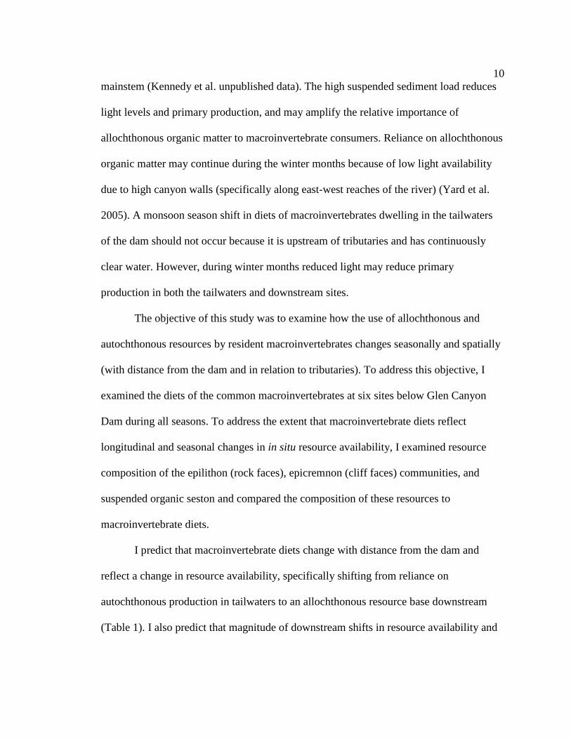
The relative importance of in situ algal production in the tailwaters or
allochthonous inputs from tributaries in supporting macroinvertebrate production, has not
been extensively studied, but hypotheses on the form of these relationships can be
formulated (Figure 1). The completion of the Glen Canyon Dam in 1963 substantially
reduced sediment loads in the river, increasing light levels and algal production in the
9
tailwaters below the dam and downstream (Stevens et al. 1997). In addition, organic
matter inputs from upstream were reduced. Downstream tributaries increase turbidity
which reduces light levels and algal production (Yard 2003, Hall et al. unpublished data).
But tributaries are also a source of allochthonous organic matter into the mainstem
Colorado River and can dominate downstream carbon budgets (Kennedy et al.
unpublished data) (Figure 1). Stable isotope food-web analysis by Angradi (1994)
indicates that aquatic secondary production in Glen Canyon (tailwaters) is fueled by
autochthonous carbon, but terrestrial riparian and upland vegetation may be important to
downstream food webs. Therefore, the organic matter budget in the river shifts
longitudinally from autochthonous to allochthonous resources (Kennedy et al.
unpublished data) and food resources consumed by macroinvertebrates may shift
accordingly. This has been demonstrated in other systems ranging from headwaters to
large rivers (Vannote et al. 1980, Tavares-Cromar and Williams 1996, Benke and
Wallace 1997, Hall et al. 2000, Hall et al. 2001, Rosi-Marshall and Wallace 2002, Cross
et al. 2007).
Seasonal changes in resource availability due to monsoon tributary flooding in the
autumn and lower light availability in the winter may amplify the longitudinal change in
resource use by macroinvertebrates. For example, in the Little Tennessee River,
macroinvertebrate diets reflected spatial and seasonal changes in resource availability
(Rosi-Marshall and Wallace 2002). In the Colorado River basin, the Arizona monsoon
season (July to September) brings high precipitation to the basin, and increases tributary
flooding and suspended sediment and allochthonous organic matter inputs to the
10
mainstem (Kennedy et al. unpublished data). The high suspended sediment load reduces
light levels and primary production, and may amplify the relative importance of
allochthonous organic matter to macroinvertebrate consumers. Reliance on allochthonous
organic matter may continue during the winter months because of low light availability
due to high canyon walls (specifically along east-west reaches of the river) (Yard et al.
2005). A monsoon season shift in diets of macroinvertebrates dwelling in the tailwaters
of the dam should not occur because it is upstream of tributaries and has continuously
clear water. However, during winter months reduced light may reduce primary
production in both the tailwaters and downstream sites.
The objective of this study was to examine how the use of allochthonous and
autochthonous resources by resident macroinvertebrates changes seasonally and spatially
(with distance from the dam and in relation to tributaries). To address this objective, I
examined the diets of the common macroinvertebrates at six sites below Glen Canyon
Dam during all seasons. To address the extent that macroinvertebrate diets reflect
longitudinal and seasonal changes in in situ resource availability, I examined resource
composition of the epilithon (rock faces), epicremnon (cliff faces) communities, and
suspended organic seston and compared the composition of these resources to
macroinvertebrate diets.
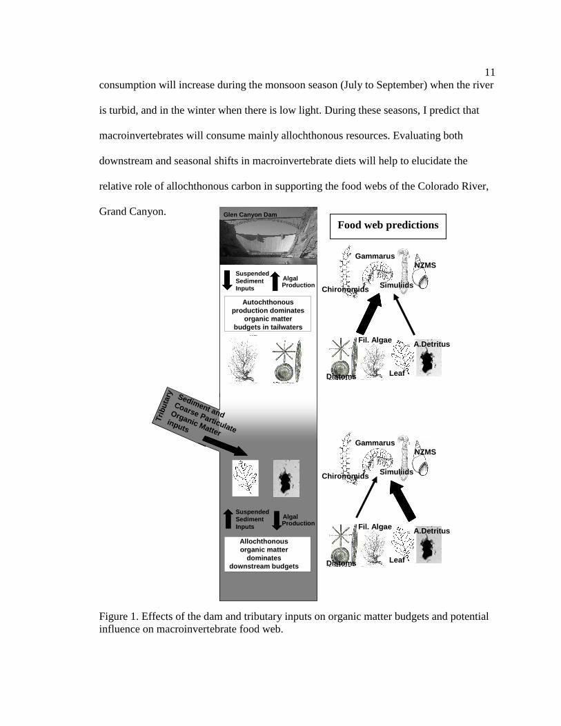
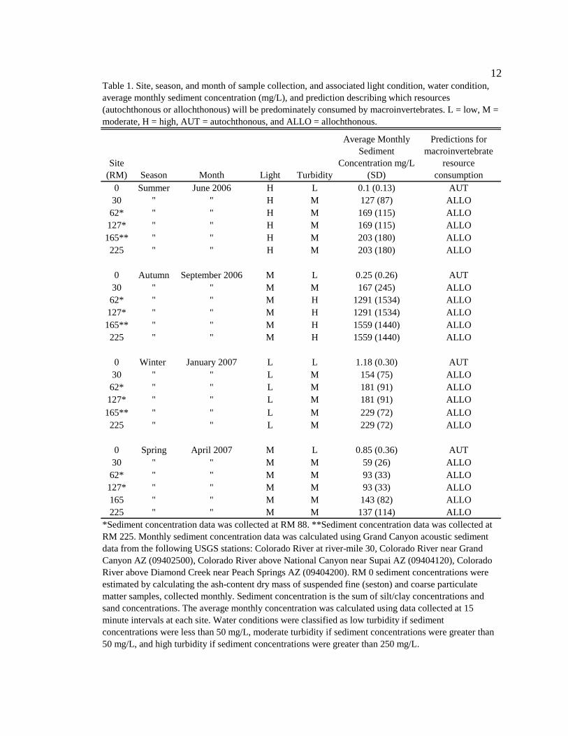
I predict that macroinvertebrate diets change with distance from the dam and
reflect a change in resource availability, specifically shifting from reliance on
autochthonous production in tailwaters to an allochthonous resource base downstream
(Table 1). I also predict that magnitude of downstream shifts in resource availability and
11
Production
Trib
utar
y
Algal
Glen Canyon Dam
SuspendedSediment Inputs
Diatoms Leaf
Gammarus
A.DetritusFil. Algae
SimuliidsChironomids
NZMS
Diatoms Leaf
Gammarus
A.DetritusFil. Algae
Simuliids
NZMS
Chironomids
ProductionAlgal
SuspendedSediment Inputs
Allochthonous organic matter
dominates downstream budgets
Sediment and Coarse Particulate
Organic Matter
inputs
Autochthonous production dominates
organic matter budgets in tailwaters
consumption will increase during the monsoon season (July to September) when the river
is turbid, and in the winter when there is low light. During these seasons, I predict that
macroinvertebrates will consume mainly allochthonous resources. Evaluating both
downstream and seasonal shifts in macroinvertebrate diets will help to elucidate the
relative role of allochthonous carbon in supporting the food webs of the Colorado River,
Grand Canyon.
Figure 1. Effects of the dam and tributary inputs on organic matter budgets and potential influence on macroinvertebrate food web.
Food web predictions
12
Site (RM) Season Month Light Turbidity
Average Monthly Sediment
Concentration mg/L (SD)
Predictions for macroinvertebrate
resource consumption
0 Summer June 2006 H L 0.1 (0.13) AUT30 " " H M 127 (87) ALLO62* " " H M 169 (115) ALLO127* " " H M 169 (115) ALLO165** " " H M 203 (180) ALLO225 " " H M 203 (180) ALLO
0 Autumn September 2006 M L 0.25 (0.26) AUT30 " " M M 167 (245) ALLO62* " " M H 1291 (1534) ALLO127* " " M H 1291 (1534) ALLO165** " " M H 1559 (1440) ALLO225 " " M H 1559 (1440) ALLO
0 Winter January 2007 L L 1.18 (0.30) AUT30 " " L M 154 (75) ALLO62* " " L M 181 (91) ALLO127* " " L M 181 (91) ALLO165** " " L M 229 (72) ALLO225 " " L M 229 (72) ALLO
0 Spring April 2007 M L 0.85 (0.36) AUT30 " " M M 59 (26) ALLO62* " " M M 93 (33) ALLO127* " " M M 93 (33) ALLO165 " " M M 143 (82) ALLO225 " " M M 137 (114) ALLO
*Sediment concentration data was collected at RM 88. **Sediment concentration data was collected at RM 225. Monthly sediment concentration data was calculated using Grand Canyon acoustic sediment data from the following USGS stations: Colorado River at river-mile 30, Colorado River near Grand Canyon AZ (09402500), Colorado River above National Canyon near Supai AZ (09404120), Colorado River above Diamond Creek near Peach Springs AZ (09404200). RM 0 sediment concentrations were estimated by calculating the ash-content dry mass of suspended fine (seston) and coarse particulate matter samples, collected monthly. Sediment concentration is the sum of silt/clay concentrations and sand concentrations. The average monthly concentration was calculated using data collected at 15 minute intervals at each site. Water conditions were classified as low turbidity if sediment concentrations were less than 50 mg/L, moderate turbidity if sediment concentrations were greater than 50 mg/L, and high turbidity if sediment concentrations were greater than 250 mg/L.
Table 1. Site, season, and month of sample collection, and associated light condition, water condition, average monthly sediment concentration (mg/L), and prediction describing which resources (autochthonous or allochthonous) will be predominately consumed by macroinvertebrates. L = low, M = moderate, H = high, AUT = autochthonous, and ALLO = allochthonous.
13
Methods
Study sites and sampling protocol
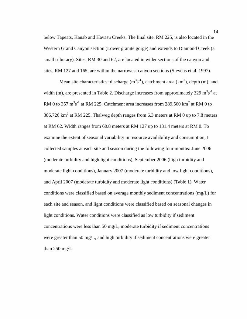
This study was conducted in the Colorado River (CR) in Grand Canyon, Arizona
(36° 03'N, 112° 09' W). Six sites were sampled over a 226 mile (363 km) reach
downstream of Glen Canyon Dam (GCD) (Figure 2). The use of river miles is the
historical precedent for describing distance along the Colorado River in Grand Canyon;
therefore, I report distances in miles, with kilometers in parentheses. Sites were selected
based on general canyon characteristics, the location of major tributary inputs, prevalence
of humpback chub populations (RM 62 and 127), and based on their long-term use as
sediment and geomorphology monitoring sites (RM 30, 62 and 127). The first site, Lee’s
Ferry (RM 0) is located in Glen Canyon and encompasses a 15.7 mile (25 km) reach
extending from the downstream end of the Glen Canyon Dam to Lee’s Ferry. This
tailwater reach is above the confluence of the Paria River, and is consistently low in
turbidity. The five downstream sites are located in the Grand Canyon, from Marble
Canyon to Diamond Creek. The second site, RM 30, is located in the Marble Canyon
section (Redwall gorge reach) of the Grand Canyon, approximately 29 miles downstream
of the Paria River, the first major tributary below the dam. The third site, RM 62, is
located in the beginning of the Central Grand Canyon section (Furnace flats reach) below
the Little Colorado River (LCR), the largest tributary. The fourth site, RM 127, is also
located in the Central Grand Canyon section (Middle granite gorge reach) below a
number of smaller tributaries including Bright Angel, Shinumo and Fossil Creeks. The
fifth site, RM 165, is located in the Western Grand Canyon section (Lower canyon reach)
14
below Tapeats, Kanab and Havasu Creeks. The final site, RM 225, is also located in the
Western Grand Canyon section (Lower granite gorge) and extends to Diamond Creek (a
small tributary). Sites, RM 30 and 62, are located in wider sections of the canyon and
sites, RM 127 and 165, are within the narrowest canyon sections (Stevens et al. 1997).
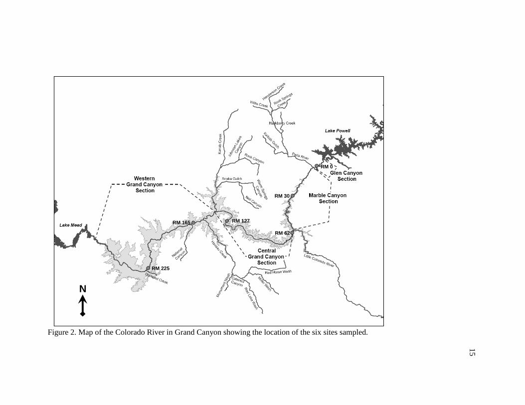
Mean site characteristics: discharge (m3s-1), catchment area (km2), depth (m), and
width (m), are presented in Table 2. Discharge increases from approximately 329 m3s-1 at
RM 0 to 357 m3s-1 at RM 225. Catchment area increases from 289,560 km2 at RM 0 to
386,726 km2 at RM 225. Thalweg depth ranges from 6.3 meters at RM 0 up to 7.8 meters
at RM 62. Width ranges from 60.8 meters at RM 127 up to 131.4 meters at RM 0. To
examine the extent of seasonal variability in resource availability and consumption, I
collected samples at each site and season during the following four months: June 2006
(moderate turbidity and high light conditions), September 2006 (high turbidity and
moderate light conditions), January 2007 (moderate turbidity and low light conditions),
and April 2007 (moderate turbidity and moderate light conditions) (Table 1). Water
conditions were classified based on average monthly sediment concentrations (mg/L) for
each site and season, and light conditions were classified based on seasonal changes in
light conditions. Water conditions were classified as low turbidity if sediment
concentrations were less than 50 mg/L, moderate turbidity if sediment concentrations
were greater than 50 mg/L, and high turbidity if sediment concentrations were greater
than 250 mg/L.
15
RM 0
RM 62
RM 30
RM 127RM 165
RM 225
N
Figure 2. Map of the Colorado River in Grand Canyon showing the location of the six sites sampled.
16
Table 2. Mean site characteristics.
Site
Annual Discharge
m3/s (SD)
Catchment area
(km2)Depth (m)
Width (m)
RM 0 329.89(53.61) 289,560 6.3 131.4
RM 30 N/A N/A 6.3 77.1
RM 60 7.8 110.3
RM 125 5.1 60.8
RM 165 NA 383,139 6.2 74.4
RM 225 357.66 (48.90) 386,726 6.8 82.5
* Site is located at RM 88. Annual discharge and catchment area were calculated using USGS Real-Time Water Data for Arizona. Annual discharge is calculated from the monthly mean discharges taken from June 2006 to May 2007. Catchment area is taken from the USGS station closest to the sites listed above. Average width and thalweg
depth were estimated at a discharge of 226 m3/s.
> 346.68 (51.45)* > 366,742*
Resource and macroinvertebrate collection
Suspended fine particulate organic matter (seston) composition samples (two to
three per site and date) were collected from the thalweg at each site by sieving river water
through a 250-µm sieve and filtering ca. 40-300 ml onto 0.45-µm gridded Metricel®
membrane filters (Pall Corp., Ann Arbor, MI). Epilithic biofilms were scraped from two
to three rocks collected from the river bed and from two to three cliff faces, using a
scraping sucking device. A 30-40 ml subsample of biofilm slurry from individual rocks
and cliffs was preserved in the field with Lugol’s solution (Prescott 1978).
Macroinvertebrates were haphazardly collected throughout the reaches of the six sites,
preserved in Kahle’s solution (Stehr 1987) in the field, and returned to the lab for gut-
content analysis.
17
Resource composition slide preparation
For epilithic and epicremnic biofilms, I filtered 0.1-5.0 ml subsamples from
preserved field collections onto gridded Metricel® membrane filters (25 mm, 0.45 µm)
(Pall Corp., Ann Arbor, MI). Seston, epilithic and epicremnic filters were mounted on
slides for preservation using Type B immersion oil.
Macroinvertebrate slide preparation
Macroinvertebrate resource consumption was measured using gut-content
analysis (Benke and Wallace 1980, Rosi-Marshall and Wallace 2002, Hall et al. 2000). I
examined diets from each of the dominant taxa [Simulium arcticum (Insecta: Diptera:
Simuliidae), Gammarus lacustris (Crustacea: Amphipoda: Gammaridae), chironomids
(Insecta: Diptera: Chironomidae), and Potamopyrgus antipodarum (New Zealand mud
snails; Gastropoda: Neotaenioglossa: Hydrobiidae)]. Dissected gut contents were drawn
onto gridded Metricel® membrane filters (25mm, 0.45µm) (Pall Corp., Ann Arbor, MI)
and mounted on slides for preservation using Type B immersion oil. Macroinvertebrates
varied in size and gut fullness; therefore, to ensure that a sufficient number of particles
were present on each prepared slide, the gut contents of one to four macroinvertebrates
were filtered onto each slide. Two to four slides were analyzed for each taxon at each site
and season.
Microscopy
A minimum of 50 individual particles on each slide were identified and their area
was measured along random transects using image analysis software, ImagePro Plus®
(Media Cybernetics Inc., Bethesda, MD), attached to a compound microscope at 100x
18
magnification (Rosi-Marshall and Wallace 2002). Particles were identified and
categorized as: diatoms, filamentous algae, leaf material, fungi, macrophyte, animal
material, cyanobacteria, red algae, and amorphous detritus (i.e. aggregations of organic
subcellular-sized particles with no recognizable cellular structure [Bowen 1984, Mann
1988, Hall et al. 2000]). The area of each particle was measured and the proportion of
each food resource in the seston, biofilms and diets was calculated.
Relative contribution of food types to production
Because food resources vary in quality, food-specific assimilation efficiencies
(percentage of a food type that a macroinvertebrate is able to assimilate) and net
production efficiencies (an estimate of the ratio of tissue production to energy
assimilation) were used to estimate the relative contribution of food types to production.
The assimilation efficiencies (AE) used were as follows: 30% for diatoms and
filamentous algae; 50% for fungi; 10% for amorphous detritus, macrophytes, leaf
material and cyanobacteria; and 70% for animal (Benke and Wallace 1980). Because I
did not measure production efficiencies for the species in this study, I assumed a net
production efficiency (NPE) of 0.5, based on the available literature (Benke and Wallace
1980). For each food resource the relative contribution (RC) of the food type (Gfood type
a….n) to production was calculated as follows:
RC = (Ga) × AE × NPE/ Σ (G(a+b+c…n) × AE ×NPE).
Estimating the origin of amorphous detritus
A common food resource for macroinvertebrates in many large river systems,
including the Colorado River, is amorphous detritus (Benke and Wallace 1997, Stevens et
19
al. 1997, Rosi-Marshall and Wallace 2002). Amorphous detritus can be autochthonously
and/or allochthonously derived because it is often formed via flocculation of dissolved
organic matter (DOM) and may be composed of: bacteria, microbes, exopolymeric
secretions from bacteria, algae and fungi, sediment particles, and small detrital fragments
(Mann 1988, Decho and Moriarty1990, Carlough 1994, Hall et al. 2000, Hart and
Lovvorn 2003). In the Colorado River, autochthonous production is high in the tailwater
reach and inputs of tributary allochthonous carbon increase downstream. Therefore,
amorphous detritus may shift from being autochthonously derived in the tailwater to
allochthonously derived downstream. Based on this observation, I assumed that all
amorphous detritus in the tailwaters is derived from algae, and I used the ratio of
amorphous detritus to diatoms in tailwater epilithic biofilms to calculate the
autochthonous fraction (AF) of amorphous detritus in downstream macroinvertebrate
diets. I calculated AF for each season, and used season-specific ratios developed from the
tailwaters to estimate the fraction of amorphous detritus that was autochthonous at the
downstream sites. For each macroinvertebrate diet, I calculated the AF of amorphous
detritus based on the percent diatoms in the diet.
I applied adjusted amorphous detritus proportions to estimate the relative
contribution of autochthonous (diatoms + filamentous algae + autochthonously derived
amorphous detritus) versus allochthonous (leaf material + allochthonously derived
amorphous detritus) resources to the production of each macroinvertebrate taxon.
Seasonal estimates for each taxon were averaged to estimate the relative contribution of
autochthonous and allochthonous resources to production over the course of the year. To

20
compare the downstream system to the tailwaters, I averaged the allochthonous and
autochthonous resource consumption by each taxon at downstream sites.
Statistical analyses
Statistical analyses were performed using the software package Systat® (v. 10.0)
(SSI San Jose, California). I compared proportions of dominant food resources consumed
by macroinvertebrates (diatoms, filamentous algae, amorphous detritus and leaf material),
among sites and seasons, using two-way analysis of variance (ANOVA). Differences in
proportions of particle types comprising seston, rock faces, and cliff faces were also
analyzed using two-way ANOVA. All proportions were arcsine-square-root transformed
before analysis to meet the normality assumption for ANOVA. When two-way ANOVA
analyses resulted in a significant site × season interaction, I analyzed each factor
independently by site or season using one-way ANOVA and Tukey’s HSD test. For
consistent reporting and analysis of the results, statistical analyses that did not result in a
significant interaction were also analyzed using one-way ANOVA and Tukey’s HSD test.
For one-way ANOVA analyses, a Bonferroni-adjusted p-value of 0.05/4 = 0.0125 was
used to compare proportions for dominant particle types among sites for each season (n =
4), and a p-value of 0.05/6 = 0.0083 was used to compare proportions among seasons for
each site (n = 6).
Characterization of resources – correlation analysis
I used correlation analysis to assess the degree of correspondence between
macroinvertebrate diets and the availability of food resources in the river. For each of the
dominant particle types (diatoms, filamentous algae, amorphous detritus and leaf
21
material), I examined the relationship between percent composition of the particle type in
a particular feeding habitat (seston, rock and cliff face biofilms) and percent consumption
of the particle type by each taxon, at each site and season. For example, the percent
diatoms in the seston at each site during each season were compared to the percent
diatoms in the gut contents of S. arcticum collected concurrently. Pearson product-
moment correlation coefficient (r) was used to assess the strength of the association
between the two variables (or the strength of the linear dependence).
Results
For clarity, the dominant patterns observed are discussed in each section of the
results and significant differences (p-values, F, and degrees of freedom) are reported in
appendices. I calculated the fraction of autochthonously derived amorphous detritus (AF)
at downstream sites, to be less than 37 percent during all seasons. Therefore, when I refer
to amorphous detritus in the results, I consider it an allochthonous resource. However, the
calculated autochthonous and allochthonous fractions of amorphous detritus were applied
to the production attributable results.
Composition of available resources
Suspended organic seston
Suspended organic seston composition was dominated by autochthonous
resources (diatoms + filamentous algae) in the clear tailwater reach (RM 0) during all
seasons (Figure 3, Table 3, Appendix 1 and 2). Along downstream reaches (RM 30 – RM
225), suspended organic seston was dominated by allochthonous resources (amorphous
detritus + leaf material) in all seasons expect during moderate turbidity conditions in
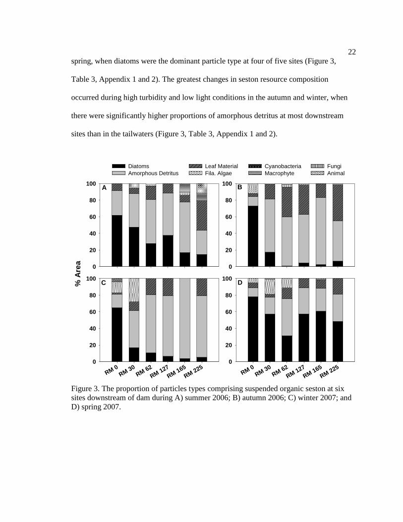
22
spring, when diatoms were the dominant particle type at four of five sites (Figure 3,
Table 3, Appendix 1 and 2). The greatest changes in seston resource composition
occurred during high turbidity and low light conditions in the autumn and winter, when
there were significantly higher proportions of amorphous detritus at most downstream
sites than in the tailwaters (Figure 3, Table 3, Appendix 1 and 2).
Figure 3. The proportion of particles types comprising suspended organic seston at six sites downstream of dam during A) summer 2006; B) autumn 2006; C) winter 2007; and D) spring 2007.
RM 0RM 30
RM 62RM 127
RM 165RM 225
0
20
40
60
80
100
RM 0RM 30
RM 62RM 127
RM 165RM 225
0
20
40
60
80
100
0
20
40
60
80
100
0
20
40
60
80
100A B
C D% A
rea
Cyanobacteria Macrophyte
DiatomsAmorphous Detritus
Leaf Material Fila. Algae
Fungi Animal

23
Season Food Resource SiteSummer RM 0 RM 30 RM 62 RM 127 RM 165 RM 225
A. Detritus 0.28 (0.01) 0.40 (N/A) 0.53 (N/A) 0.48 (0.08) 0.63 (0.05) 0.49 (0.10)Diatoms 0.62 (0.01) 0.48 (N/A) 0.28 (N/A) 0.22 (0.07) 0.15 (0.02) 0.21 (0.05)Leaves 0.10 (0.01) 0.07 (N/A) 0.16 (N/A) 0.08 (0.03) 0.11 (0.01) 0.24 (0.06)Fila. Algae 0.00 0.00 0.03 (N/A) 0.17 (0.17) 0.01 (0.01)0.00Cyanobacteria 0.00 0.00 0.00 0.00 0.00 0.00Macrophyte 0.00 0.00 0.00 0.00 0.04 (0.03) 0.03 (0.03)Fungi 0.00 0.00 0.00 0.00 0.00 0.00Animal 0.00 0.05 (N/A) 0.00 0.05 (0.05) 0.06 (0.06) 0.03 (0.04)Red Algae 0.00 0.00 0.00 0.00 0.00 0.00
Autumn A. Detritus 0.11 (0.04) 0.64 (0.02) 0.59 (0.05) 0.58 (0.03) 0.81 (0.03) 0.48 (0.03)Diatoms 0.73 (0.10) 0.17 (0.05) 0.01 (0.003) 0.05 (0.02) 0.02 (0.01) 0.07 (0.01)Leaves 0.04 (0.03) 0.18 (0.07) 0.36 (0.07) 0.35 (0.03) 0.17 (0.02) 0.44 (0.03)Fila. Algae 0.12 (0.07) 0.00 0.00 0.01 (0.01) 0.00 0.00Cyanobacteria 0.00 0.00 0.00 0.00 0.00 0.00Macrophyte 0.00 0.00 0.00 0.00 0.00 0.00Fungi 0.00 0.01 (0.005) 0.04 (0.04) 0.01 (0.005) 0.00 0.01 (0.01)Animal 0.00 0.00 0.00 0.00 0.00 0.00Red Algae 0.00 0.00 0.00 0.00 0.00 0.00
Winter A. Detritus 0.21 (0.02) 0.45 (0.05) 0.58 (0.10) 0.72 (0.02) 0.77 (0.09) 0.72 (0.03)Diatoms 0.67 (0.01) 0.21 (0.02) 0.10 (0.01) 0.07 (0.04)0.03 (0.01) 0.08 (0.01)Leaves 0.07 (0.03) 0.18 (0.04) 0.32 (0.10) 0.21 (0.02) 0.20 (0.10) 0.20 (0.03)Fila. Algae 0.05 (0.05) 0.16 (0.08) 0.00 0.00 0.00 0.00Cyanobacteria 0.00 0.00 0.00 0.00 0.00 0.00Macrophyte 0.00 0.00 0.00 0.00 0.00 0.00Fungi 0.00 0.00 0.00 0.00 0.00 0.00Animal 0.00 0.00 0.00 0.00 0.00 0.00Red Algae 0.00 0.00 0.00 0.00 0.00 0.00
Spring A. Detritus 0.13 (0.03) 0.18 (0.01) 0.42 (0.02) 0.24 (0.04) 0.40 (0.09) 0.36 (0.03)Diatoms 0.81 (0.03) 0.70 (0.06) 0.38 (0.07) 0.60 (0.04)0.54 (0.08) 0.46 (0.03)Leaves 0.04 (0.01) 0.03 (0.01) 0.10 (0.01) 0.16 (0.04) 0.06 (0.02) 0.18 (0.002)Fila. Algae 0.02 (0.01) 0.08 (0.04) 0.07 (0.03) 0.00 0.00 0.00Cyanobacteria 0.00 0.00 0.00 0.00 0.00 0.00Macrophyte 0.00 0.01 (0.003) 0.00 0.00 0.00 0.00Fungi 0.00 0.00 0.00 0.00 0.00 0.00Animal 0.00 0.00 0.03 (0.03) 0.00 0.00 0.00Red Algae 0.00 0.00 0.00 0.00 0.00 0.00
Table 3. Mean (SE) proportion of particle types comprising suspended organic seston for each site and season.
Epilithon (rock faces)
Epilithic biofilms in the tailwater reach (RM 0) were dominated by autochthonous
resources (diatoms + filamentous algae) during all seasons (Table 4, Appendix 3 and 4).
24
Along downstream reaches, epilithic biofilms were dominated by allochthonous
resources (amorphous detritus + leaf material) during all seasons except during moderate
turbidity conditions in summer and spring, when diatoms comprised the greatest
proportion of the biofilm for the upper most reach (RM 30) in summer, and the two upper
reaches (RM 30 and RM 62) in spring (Table 4, Appendix 3 and 4). Consistent
significant differences in the proportion of particle types comprising epilithic biofilms
were only present for filamentous algae, with higher proportions of filamentous algae in
the tailwaters than downstream sites, during moderate turbidity conditions in the summer
and winter (Table 4, Appendix 3 and 4).
Epicremnon (cliff faces)
Epicremnic biofilms in the tailwater reach (RM 0) were dominated by
autochthonous resources (diatoms + filamentous algae) during all seasons except during
moderate turbidity/low light conditions in winter, when amorphous detritus was the
dominant particle type (Table 5, Appendix 5 and 6). Along downstream reaches (RM 30
– RM 225), epicremnic biofilms were dominated by allochthonous resources except
during moderate turbidity conditions in summer and spring, when diatoms were the
dominant particle type for the upper most reach (RM 30) in the spring, and the two upper
reaches (RM 30 and 62) in the summer (Table 5, Appendix 5 and 6).
25
Season Food Resource SiteSummer RM 0 RM 30 RM 62 RM 127 RM 165 RM 225
A. Detritus 0.09 (0.02) 0.28 (0.06) 0.58 (0.17) 0.52 (0.17) 0.54 (0.17) 0.79 (0.05)Diatoms 0.65 (0.07) 0.58 (0.10) 0.34 (0.13) 0.16 (0.09)0.32 (0.20) 0.08 (0.03)Leaves 0.002 (0.001) 0.11 (0.02) 0.08 (0.04) 0.30 (0.16) 0.14 (0.03) 0.12 (0.05)Fila. Algae 0.25 (0.08) 0.001 (0.001) 0.00 0.00 0.00 0.00Cyanobacteria 0.00 0.00 0.00 0.00 0.00 0.00Macrophyte 0.00 0.00 0.00 0.00 0.00 0.00Fungi 0.003 (0.003) 0.03 (0.03) 0.00 0.02 (0.02) 0.00 0.01 (0.01)Animal 0.01 (0.01) 0.00 0.00 0.00 0.00 0.00Red Algae 0.00 0.00 0.00 0.00 0.00 0.00
Autumn A. Detritus 0.11 (0.01) 0.76 (0.02) 0.75 (0.02) 0.84 (0.11) 0.64 (0.05) 0.49 (0.20)Diatoms 0.82 (0.04) 0.21 (0.03) 0.24 (0.02) 0.13 (0.11)0.33 (0.07) 0.37 (0.26)Leaves 0.01 (0.01) 0.03 (0.02) 0.01 (0.003) 0.03 (0.01)0.03 (0.03) 0.14 (0.11)Fila. Algae 0.04 (0.04) 0.00 0.00 0.00 0.00 0.00Cyanobacteria 0.00 0.00 0.00 0.00 0.00 0.00Macrophyte 0.02 (0.01) 0.00 0.00 0.00 0.00 0.00Fungi 0.00 0.00 0.00 0.00 0.00 0.00Animal 0.00 0.00 0.00 0.00 0.00 0.00Red Algae 0.00 0.00 0.00 0.00 0.00 0.00
Winter A. Detritus 0.24 (0.09) 0.53 (0.06) 0.72 (0.05) 0.68 (0.11) 0.56 (0.12) 0.47 (0.23)Diatoms 0.62 (0.08) 0.30 (0.04) 0.15 (0.02) 0.07 (0.05)0.09 (0.05) 0.26 (0.25)Leaves 0.04 (0.01) 0.17 (0.05) 0.11 (0.03) 0.24 (0.05) 0.24 (0.06) 0.19 (0.04)Fila. Algae 0.10 (0.02) 0.00 0.02 (0.01) 0.00 0.01 (0.01) 0.01 (0.005)Cyanobacteria 0.00 0.00 0.00 0.00 0.00 0.00Macrophyte 0.00 0.00 0.00 0.00 0.00 0.00Fungi 0.001 (0.001) 0.00 0.00 0.01 (0.01) 0.10 (0.10) 0.0002 (0.0002)Animal 0.00 0.00 0.00 0.00 0.00 0.00Red Algae 0.00 0.00 0.00 0.00 0.00 0.07 (0.08)
Spring A. Detritus 0.04 (0.03) 0.29 (0.09) 0.36 (0.03) 0.50 (0.11) 0.49 (0.14) 0.33 (0.02)Diatoms 0.62 (0.14) 0.67 (0.08) 0.50 (0.10) 0.44 (0.12)0.33 (0.15) 0.33 (0.05)Leaves 0.01 (0.005) 0.04 (0.004) 0.07 (0.01) 0.06 (0.01) 0.09 (0.05) 0.29 (0.08)Fila. Algae 0.25 (0.16) 0.00 0.04 (0.02) 0.00 0.09 (0.09) 0.00Cyanobacteria 0.00 0.00 0.00 0.00 0.00 0.00Macrophyte 0.08 (0.08) 0.00 0.00 0.00 0.00 0.05 (0.05)Fungi 0.001 (0.001) 0.00 0.03 (0.03) 0.00 0.00 0.00Animal 0.00 0.00 0.00 0.00 0.00 0.00Red Algae 0.00 0.00 0.00 0.00 0.00 0.00
Table 4. Mean (SE) proportion of particle types comprising epilithon for each site and season.
26
Season Food Resource SiteSummer RM 0 RM 30 RM 62 RM 127 RM 165 RM 225
A. Detritus 0.04 (0.002) 0.18 (0.08) 0.37 (N/A) 0.54 (0.02) 0.49 (0.13) 0.67 (0.05)Diatoms 0.78 (0.03) 0.72 (0.13) 0.55 (N/A) 0.11 (0.05) 0.06 (0.06) 0.00Leaves 0.01 (0.003) 0.10 (0.05) 0.08 (N/A) 0.29 (0.10) 0.25 (0.06) 0.33 (0.05)Fila. Algae 0.17 (0.03) 0.00 0.00 0.00 0.00 0.00Cyanobacteria 0.00 0.00 0.00 0.00 0.00 0.00Macrophyte 0.00 0.00 0.00 0.00 0.00 0.00Fungi 0.00 0.00 0.00 0.06 (0.06) 0.20 (0.20) 0.00Animal 0.00 0.00 0.00 0.00 0.00 0.00Red Algae 0.00 0.00 0.00 0.00 0.00 0.00
Autumn A. Detritus 0.25 (0.09) 0.64 (0.04) 0.53 (N/A) 0.79 (0.09) 0.80 (0.103) 0.93 (0.02)Diatoms 0.64 (0.06) 0.34 (0.05) 0.43 (N/A) 0.01 (0.01) 0.13 (0.11) 0.02 (0.02)Leaves 0.04 (0.01) 0.02 (0.01) 0.04 (N/A) 0.11 (0.07) 0.02 (0.01) 0.05 (0.01)Fila. Algae 0.04 (0.04) 0.00 0.00 0.09 (0.09) 0.05 (0.05) 0.00Cyanobacteria 0.00 0.00 0.00 0.00 0.00 0.00Macrophyte 0.00 0.00 0.00 0.00 0.00 0.00Fungi 0.03 (0.03) 0.00 0.00 0.00 0.00 0.00Animal 0.00 0.00 0.00 0.00 0.00 0.00Red Algae 0.00 0.00 0.00 0.00 0.00 0.00
Winter A. Detritus 0.50 (0.15) 0.61 (0.01) 0.74 (0.03) 0.48 (0.10) 0.49 (0.06) 0.57 (0.18)Diatoms 0.39 (0.16) 0.07 (0.05) 0.03 (0.01) 0.26 (0.16)0.22 (0.09) 0.05 (0.03)Leaves 0.05 (0.02) 0.32 (0.03) 0.23 (0.02) 0.23 (0.06) 0.26 (0.04) 0.19 (0.04)Fila. Algae 0.05 (0.02) 0.00 0.00 0.03 (0.03) 0.03 (0.03) 0.00Cyanobacteria 0.00 0.00 0.00 0.00 0.00 0.00Macrophyte 0.00 0.00 0.00 0.00 0.00 0.11 (0.11)Fungi 0.01 (0.01) 0.00 0.00 0.00 0.00 0.08 (0.08)Animal 0.00 0.00 0.00 0.00 0.00 0.00Red Algae 0.00 0.00 0.00 0.00 0.00 0.00
Spring A. Detritus 0.23 (0.11) 0.30 (0.09) 0.60 (0.09) 0.52 (0.11) 0.70 (0.10) 0.57 (0.11)Diatoms 0.68 (0.14) 0.60 (0.15) 0.19 (0.06) 0.22 (0.05)0.23 (0.06) 0.26 (0.09)Leaves 0.01 (0.01) 0.10 (0.06) 0.17 (0.05) 0.20 (0.07) 0.07 (0.03) 0.15 (0.03)Fila. Algae 0.08 (0.08) 0.004 (0.004) 0.04 (0.04) 0.04 (0.04) 0.00 0.02 (0.02)Cyanobacteria 0.00 0.00 0.00 0.00 0.00 0.00Macrophyte 0.00 0.00 0.00 0.00 0.00 0.00Fungi 0.00 0.002 (0.002) 0.002 (0.002) 0.02 (0.02) 0.00 0.00Animal 0.00 0.00 0.00 0.00 0.00 0.00Red Algae 0.00 0.00 0.00 0.00 0.00 0.00
Table 5. Mean (SE) proportion of particle types comprising epicremnon for each site and season.
27
Macroinvertebrate diets
Simulium arcticum
S. arcticum consumed mainly diatoms in the tailwater reach during all seasons
(Figure 4, Table 6, Appendix 7). Along downstream reaches (RM 30 – RM 225), S.
arcticum consumed mainly allochthonous resources (amorphous detritus + leaf material)
during all seasons (Figure 4, Table 6, Appendix 7). S. arcticum diets also changed
seasonally, specifically at the sites below major tributaries (RM 30 and RM 62) (Figure 4,
Table 6, Appendix 7). During moderate turbidity conditions in the summer, winter, and
spring, S. arcticum consumed a higher proportion of diatoms (though not always
significant) at all downstream sites than during high turbidity conditions in the autumn
(Figure 4, Table 6, Appendix 8). In contrast, in the autumn S. arcticum consumed mainly
amorphous detritus at all downstream sites (Figure 4, Table 6, Appendix 8).
In the tailwaters, autochthonous organic matter (diatoms + filamentous algae +
autochthonously derived amorphous detritus) contributes the greatest amount to S.
arcticum production; contributing 99% to the average yearly (average for all four
seasons) S. arcticum production (Figure 5). At downstream sites, allochthonous organic
matter (allochthonously derived amorphous detritus + leaf material) contributes the
greatest amount to S. arcticum production; contributing 57% to the average yearly
(average for all four seasons and all five downstream sites) S. arcticum production
(Figure 5). More specifically, in the tailwaters, diatoms contribute the greatest amount to
S. arcticum production during all seasons (85%-95%, range for all seasons) (Table 7). At
downstream sites, allochthonous amorphous detritus contributes the greatest amount to S.
28
RM 0RM 30
RM 62RM 127
RM 165RM 225
0
20
40
60
80
100
RM 0RM 30
RM 62RM 127
RM 165RM 225
0
20
40
60
80
100
0
20
40
60
80
100
0
20
40
60
80
100A B
C D
N/A
% A
rea
Cyanobacteria Macrophyte
DiatomsAmorphous Detritus
Leaf Material Fila. Algae
Fungi Animal
arcticum production during high turbidity conditions in the autumn (65-93%, range for
the five downstream sites). During moderate turbidity conditions in the summer, winter,
and spring, diatoms and allochthonous amorphous detritus contribute somewhat equally
to production (Table 7). During these seasons diatoms can contribute from 27-67%
(range for the five downstream sites, during the three moderate turbidity seasons), and
allochthonous amorphous detritus can contribute from 22-64% (range for the five
downstream sites during the three moderate turbidity seasons) to S. arcticum production.
Figure 4. The proportion of particle types consumed seasonally by Simulium arcticum at six sites downstream of dam during A) summer 2006; B) autumn 2006; C) winter 2007; and D) spring 2007.

29
Season Food Resource SiteSummer RM 0 RM 30 RM 62 RM 127 RM 165 RM 225
A. Detritus 0.19 (0.03) 0.46 (0.04) 0.72 (0.03) 0.78 (0.02) 0.81 (0.03) 0.76 (0.04)Diatoms 0.79 (0.03) 0.41 (0.05) 0.27 (0.03) 0.16 (0.03)0.12 (0.01) 0.24 (0.04)Leaves 0.01 (0.01) 0.13 (0.08) 0.01 (0.004) 0.06 (0.01)0.07 (0.03) 0.002 (0.002)Fila. Algae 0.01 (0.01) 0.00 0.001 (0.001) 0.00 0.00 0.00Cyanobacteria 0.001(0.0004) 0.003 (0.001) 0.00 0.00 0.00 0.002 (0.002)Macrophyte 0.00 0.00 0.00 0.00 0.00 0.00Fungi 0.00 0.00 0.00 0.00 0.00 0.00Animal 0.00 0.00 0.00 0.00 0.00 0.00Red Algae 0.00 0.00 0.00 0.00 0.00 0.00
Autumn A. Detritus 0.12 (0.03) 0.94 (0.02) 0.97 (0.02) 0.87 (0.04) 0.75 (0.8) 0.94 (0.004)Diatoms 0.87 (0.03) 0.04 (0.01) 0.02 (0.02) 0.09 (0.05)0.05 (0.02) 0.05 (0.01)Leaves 0.001 (0.004) 0.01 (0.005) 0.01 (0.004) 0.04 (0.02) 0.18 (0.10) 0.01 (0.01)Fila. Algae 0.01 (0.004) 0.01 (0.01) 0.00 0.00 0.02 (0.02) 0.00Cyanobacteria 0.00 0.00 0.00 0.00 0.00 0.00Macrophyte 0.00 0.00 0.00 0.00 0.00 0.00Fungi 0.00 0.00 0.00 0.00 0.00 0.00Animal 0.00 0.00 0.00 0.00 0.00 0.00Red Algae 0.00 0.00 0.00 0.00 0.00 0.00
Winter A. Detritus 0.28 (0.06) 0.55 (0.14) 0.76 (0.04) 0.63 (0.13) 0.44 (0.04) 0.67 (0.05)Diatoms 0.67 (0.06) 0.23 (0.11) 0.14 (0.02) 0.15 (0.06)0.16 (0.04) 0.18 (0.04)Leaves 0.01 (0.01) 0.10 (0.03) 0.09 (0.03) 0.08 (0.02) 0.15 (0.06) 0.15 (0.02)Fila. Algae 0.004 (0.003) 0.12 (0.12) 0.01 (0.01) 0.10 (0.10) 0.17 (0.07) 0.00Cyanobacteria 0.01 (0.01) 0.00 0.00 0.00 0.07 (0.07) 0.00Macrophyte 0.02 (0.01) 0.00 0.00 0.001 (0.002) 0.00 0.00Fungi 0.003 (0.003) 0.00 0.00 0.04 (0.02) 0.01 (0.005) 0.00Animal 0.00 0.00 0.00 0.00 0.00 0.00Red Algae 0.00 0.00 0.00 0.00 0.00 0.00
Spring A. Detritus 0.15 (0.03) N/A 0.65 (0.02) 0.77 (N/A) 0.64 (0.06) 0.69 (0.07)Diatoms 0.84 (0.03) N/A 0.29 (0.03) 0.19 (N/A) 0.32 (0.06) 0.21 (0.03)Leaves 0.01 (0.002) N/A 0.03 (0.01) 0.03 (N/A) 0.03 (0.01) 0.03 (0.01)Fila. Algae 0.00 N/A 0.01 (0.01) 0.01 (N/A) 0.01 (0.01) 0.06 (0.06)Cyanobacteria 0.00 N/A 0.00 0.00 0.00 0.00Macrophyte 0.00 N/A 0.003 (0.003) 0.00 0.00 0.00Fungi 0.001 (0.001) N/A 0.00 0.00 0.002 (0.001) 0.01 (0.002)Animal 0.00 N/A 0.02 (0.01) 0.00 0.00 0.00Red Algae 0.00 N/A 0.00 0.00 0.00 0.00
Table 6. Mean (SE) proportion of consumption by Simulium arcticumfor each site and season. N/A indicates no data available.
30
RM 0
SIMGAM
NZMSCHIR
Per
cent
0
20
40
60
80
100
Downstream sites
SIMGAM
NZMSCHIR
Allochthonous Autochthonous
Figure 5. The percent of each taxon’s production attributable to autochthonous (diatoms + filamentous algae + autochthonously derived amorphous detritus) and allochthonous (leaf material + allochthonously derived amorphous detritus) resources in the tailwaters (RM 0) and at downstream sites. The percent of production attributable to autochthonous and allochthonous resources was calculated seasonally at each site. Seasonal calculations were averaged to estimate the yearly average percent attributable to resources for each taxon. Seasonal calculations for the five downstream sites were also averaged to estimate the yearly average percent attributable to resources for the downstream system.
31
Season Taxa Food Resource SiteSummer Simuliid RM 0 RM 30 RM 62 RM 127 RM 165 RM 225
Allochthonous A. Detritus 0 22 44 57 63 49Autochthonous A. Detritus 7 3 2 2 1 2Diatoms 91 67 52 36 29 49Leaves 0 7 1 5 6 0.1Fila. Algae 1 0 0.2 0 0 0Cyanobacteria 0.04 0.2 0 0 0 0.1Macrophyte 0 0 0 0 0 0Fungi 0 0 0 0 0 0Animal 0 0 0 0 0 0Red Algae 0 0 0 0 0 0
Autumn SimuliidAllochthonous A. Detritus 0 85 93 73 65 84Autochthonous A. Detritus 4 1 0.3 1 1 1Diatoms 95 10 6 23 13 14Leaves 0.04 1 1 3 16 2Fila. Algae 1 3 0 0 5 0Cyanobacteria 0 0 0 0 0 0Macrophyte 0 0 0 0 0 0Fungi 0 0 0 0 0 0Animal 0 0 0 0 0 0Red Algae 0 0 0 0 0 0
Winter SimuliidAllochthonous A. Detritus 0 27 54 34 22 44Autochthonous A. Detritus 12 5 4 3 4 5Diatoms 85 41 32 27 28 40Leaves 0.4 6 7 5 9 11Fila. Algae 0.4 21 2 18 30 0Cyanobacteria 0.4 0 0 0 4 0Macrophyte 1 0 0 0.1 0 0Fungi 1 0 0 12 3 0Animal 0 0 0 0 0 0Red Algae 0 0 0 0 0 0
Table 7. Production attributed to food type (%). Calculation: Food type in gut (%) x Assimilation efficiency (AE) x Net production efficiency (NPE)/ Σ (G(a+b+c…n) × AE ×NPE). N/A indicates no data available.
32
Season Taxa Food Resource SiteSpring Simuliid RM 0 RM 30 RM 62 RM 127 RM 165 RM 225
Allochthonous A. Detritus 0 N/A 37 54 37 43Autochthonous A. Detritus 6 N/A 1 1 1 1Diatoms 94 N/A 50 41 57 40Leaves 0.4 N/A 2 2 2 2Fila. Algae 0 N/A 2 2 2 11Cyanobacteria 0 N/A 0 0 0 0Macrophyte 0 N/A 0.2 0 0 0Fungi 0.2 N/A 0 0 1 3Animal 0 N/A 8 0 0 0Red Algae 0 N/A 0 0 0 0
Summer GammarusAllochthonous A. Detritus 0 26 52 11 N/A 46Autochthonous A. Detritus 27 3 2 4 N/A 2Diatoms 71 64 35 83 N/A 50Leaves 2 3 12 2 N/A 1Fila. Algae 0 3 0.2 0 N/A 0Cyanobacteria 0 0 0 0 N/A 0Macrophyte 0 0 0 0 N/A 0Fungi 0 0 0 0 N/A 0Animal 0 0 0 0 N/A 0Red Algae 0 0 0 0 N/A 0
Autumn Gammarus
Allochthonous A. Detritus 0 45 69 33 31 79Autochthonous A. Detritus 18 2 0 0 1 0.3Diatoms 64 38 3 5 15 5Leaves 1 9 10 6 10 6Fila. Algae 18 6 8 3 5 8Cyanobacteria 0 0 0 0 0 0Macrophyte 0 0 5 4 3 0Fungi 0 0 5 22 20 0.5Animal 0 0 0 27 16 0Red Algae 0 0 0 0 0 0
Table 7. Continued.
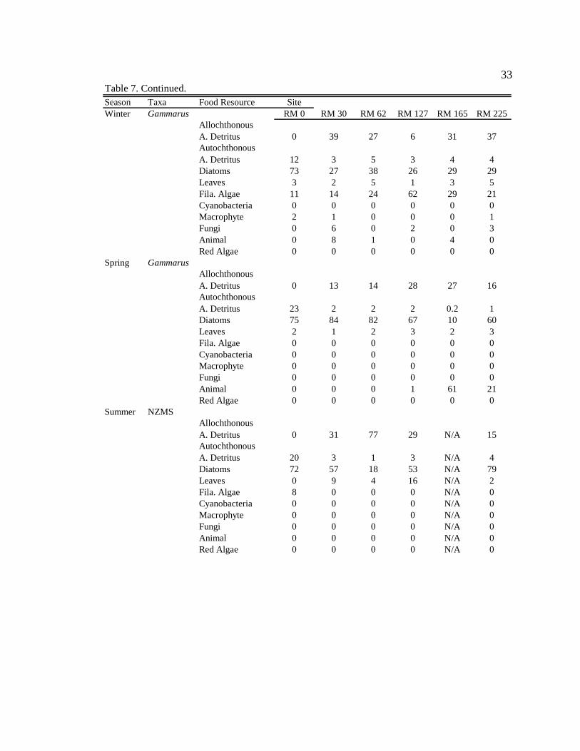
33
Season Taxa Food Resource SiteWinter Gammarus RM 0 RM 30 RM 62 RM 127 RM 165 RM 225
Allochthonous A. Detritus 0 39 27 6 31 37Autochthonous A. Detritus 12 3 5 3 4 4Diatoms 73 27 38 26 29 29Leaves 3 2 5 1 3 5Fila. Algae 11 14 24 62 29 21Cyanobacteria 0 0 0 0 0 0Macrophyte 2 1 0 0 0 1Fungi 0 6 0 2 0 3Animal 0 8 1 0 4 0Red Algae 0 0 0 0 0 0
Spring GammarusAllochthonous A. Detritus 0 13 14 28 27 16Autochthonous A. Detritus 23 2 2 2 0.2 1Diatoms 75 84 82 67 10 60Leaves 2 1 2 3 2 3Fila. Algae 0 0 0 0 0 0Cyanobacteria 0 0 0 0 0 0Macrophyte 0 0 0 0 0 0Fungi 0 0 0 0 0 0Animal 0 0 0 1 61 21Red Algae 0 0 0 0 0 0
Summer NZMSAllochthonous A. Detritus 0 31 77 29 N/A 15Autochthonous A. Detritus 20 3 1 3 N/A 4Diatoms 72 57 18 53 N/A 79Leaves 0 9 4 16 N/A 2Fila. Algae 8 0 0 0 N/A 0Cyanobacteria 0 0 0 0 N/A 0Macrophyte 0 0 0 0 N/A 0Fungi 0 0 0 0 N/A 0Animal 0 0 0 0 N/A 0Red Algae 0 0 0 0 N/A 0
Table 7. Continued.
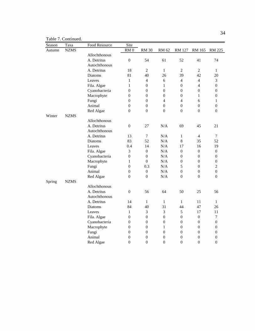
34
Season Taxa Food Resource SiteAutumn NZMS RM 0 RM 30 RM 62 RM 127 RM 165 RM 225
Allochthonous A. Detritus 0 54 61 52 41 74Autochthonous A. Detritus 18 2 1 2 2 1Diatoms 81 40 26 39 42 20Leaves 1 4 6 4 4 3Fila. Algae 1 0 1 0 4 0Cyanobacteria 0 0 0 0 0 0Macrophyte 0 0 0 0 1 0Fungi 0 0 4 4 6 1Animal 0 0 0 0 0 0Red Algae 0 0 0 0 0 0
Winter NZMSAllochthonous A. Detritus 0 27 N/A 69 45 21Autochthonous A. Detritus 13 7 N/A 1 4 7Diatoms 83 52 N/A 8 35 52Leaves 0.4 14 N/A 17 16 19Fila. Algae 3 0 N/A 0 0 0Cyanobacteria 0 0 N/A 0 0 0Macrophyte 1 0 N/A 0 0 0Fungi 0 0.3 N/A 5 0 2Animal 0 0 N/A 0 0 0Red Algae 0 0 N/A 0 0 0
Spring NZMSAllochthonous A. Detritus 0 56 64 50 25 56Autochthonous A. Detritus 14 1 1 1 11 1Diatoms 84 40 31 44 47 26Leaves 1 3 3 5 17 11Fila. Algae 0 0 0 0 0 7Cyanobacteria 0 0 0 0 0 0Macrophyte 0 0 1 0 0 0Fungi 0 0 0 0 0 0Animal 0 0 0 0 0 0Red Algae 0 0 0 0 0 0
Table 7. Continued.
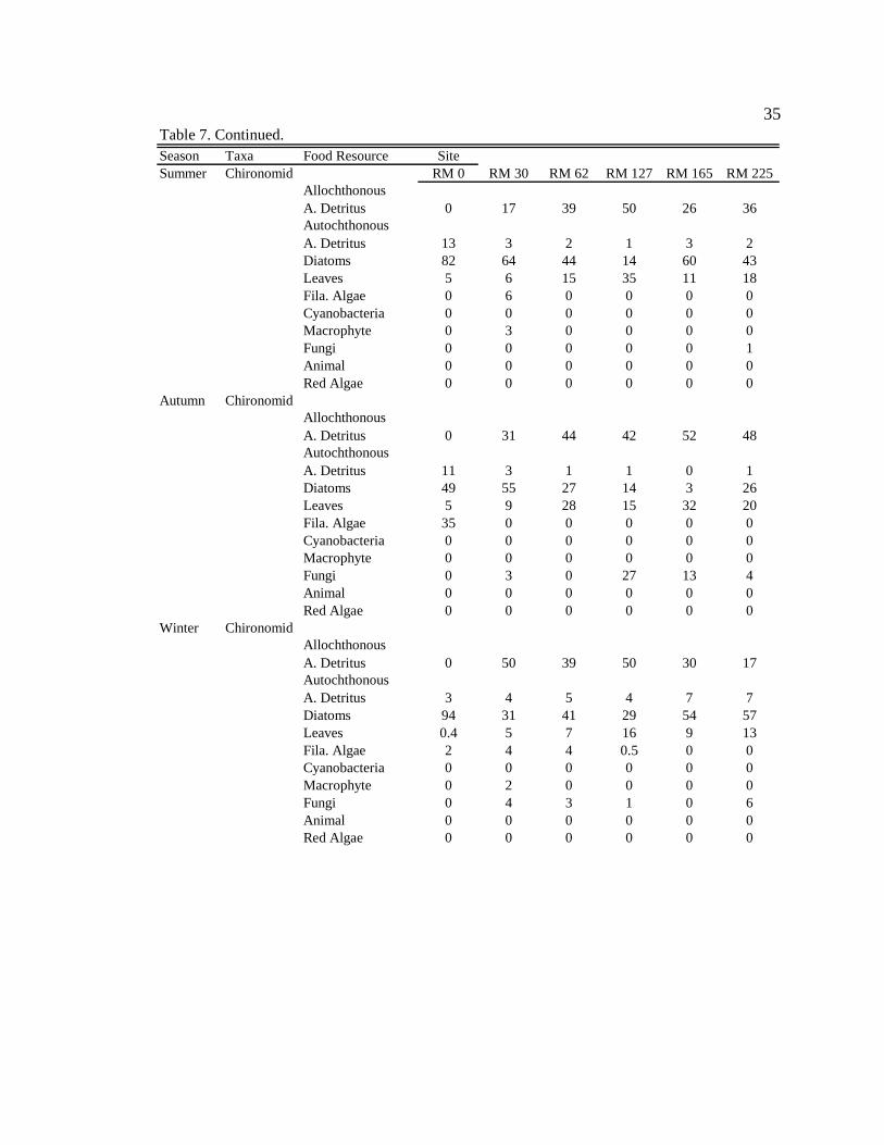
35
Season Taxa Food Resource SiteSummer Chironomid RM 0 RM 30 RM 62 RM 127 RM 165 RM 225
Allochthonous A. Detritus 0 17 39 50 26 36Autochthonous A. Detritus 13 3 2 1 3 2Diatoms 82 64 44 14 60 43Leaves 5 6 15 35 11 18Fila. Algae 0 6 0 0 0 0Cyanobacteria 0 0 0 0 0 0Macrophyte 0 3 0 0 0 0Fungi 0 0 0 0 0 1Animal 0 0 0 0 0 0Red Algae 0 0 0 0 0 0
Autumn ChironomidAllochthonous A. Detritus 0 31 44 42 52 48Autochthonous A. Detritus 11 3 1 1 0 1Diatoms 49 55 27 14 3 26Leaves 5 9 28 15 32 20Fila. Algae 35 0 0 0 0 0Cyanobacteria 0 0 0 0 0 0Macrophyte 0 0 0 0 0 0Fungi 0 3 0 27 13 4Animal 0 0 0 0 0 0Red Algae 0 0 0 0 0 0
Winter ChironomidAllochthonous A. Detritus 0 50 39 50 30 17Autochthonous A. Detritus 3 4 5 4 7 7Diatoms 94 31 41 29 54 57Leaves 0.4 5 7 16 9 13Fila. Algae 2 4 4 0.5 0 0Cyanobacteria 0 0 0 0 0 0Macrophyte 0 2 0 0 0 0Fungi 0 4 3 1 0 6Animal 0 0 0 0 0 0Red Algae 0 0 0 0 0 0
Table 7. Continued.
36
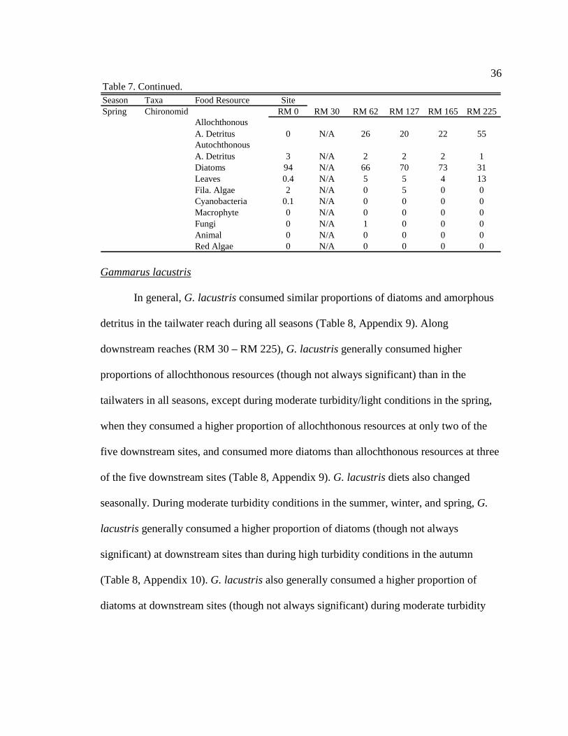
Season Taxa Food Resource SiteSpring Chironomid RM 0 RM 30 RM 62 RM 127 RM 165 RM 225
Allochthonous A. Detritus 0 N/A 26 20 22 55Autochthonous A. Detritus 3 N/A 2 2 2 1Diatoms 94 N/A 66 70 73 31Leaves 0.4 N/A 5 5 4 13Fila. Algae 2 N/A 0 5 0 0Cyanobacteria 0.1 N/A 0 0 0 0Macrophyte 0 N/A 0 0 0 0Fungi 0 N/A 1 0 0 0Animal 0 N/A 0 0 0 0Red Algae 0 N/A 0 0 0 0
Table 7. Continued.
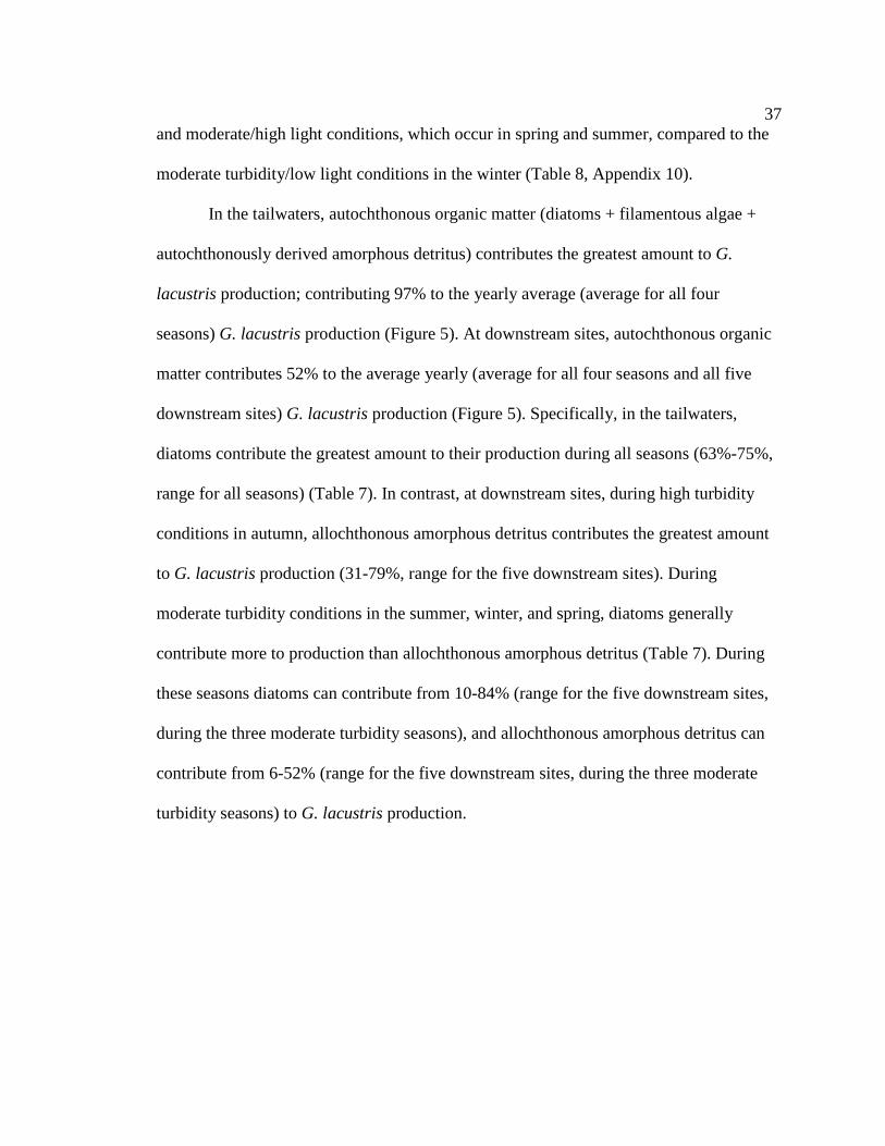
Gammarus lacustris
In general, G. lacustris consumed similar proportions of diatoms and amorphous
detritus in the tailwater reach during all seasons (Table 8, Appendix 9). Along
downstream reaches (RM 30 – RM 225), G. lacustris generally consumed higher
proportions of allochthonous resources (though not always significant) than in the
tailwaters in all seasons, except during moderate turbidity/light conditions in the spring,
when they consumed a higher proportion of allochthonous resources at only two of the
five downstream sites, and consumed more diatoms than allochthonous resources at three
of the five downstream sites (Table 8, Appendix 9). G. lacustris diets also changed
seasonally. During moderate turbidity conditions in the summer, winter, and spring, G.
lacustris generally consumed a higher proportion of diatoms (though not always
significant) at downstream sites than during high turbidity conditions in the autumn
(Table 8, Appendix 10). G. lacustris also generally consumed a higher proportion of
diatoms at downstream sites (though not always significant) during moderate turbidity
37
and moderate/high light conditions, which occur in spring and summer, compared to the
moderate turbidity/low light conditions in the winter (Table 8, Appendix 10).
In the tailwaters, autochthonous organic matter (diatoms + filamentous algae +
autochthonously derived amorphous detritus) contributes the greatest amount to G.
lacustris production; contributing 97% to the yearly average (average for all four
seasons) G. lacustris production (Figure 5). At downstream sites, autochthonous organic
matter contributes 52% to the average yearly (average for all four seasons and all five
downstream sites) G. lacustris production (Figure 5). Specifically, in the tailwaters,
diatoms contribute the greatest amount to their production during all seasons (63%-75%,
range for all seasons) (Table 7). In contrast, at downstream sites, during high turbidity
conditions in autumn, allochthonous amorphous detritus contributes the greatest amount
to G. lacustris production (31-79%, range for the five downstream sites). During
moderate turbidity conditions in the summer, winter, and spring, diatoms generally
contribute more to production than allochthonous amorphous detritus (Table 7). During
these seasons diatoms can contribute from 10-84% (range for the five downstream sites,
during the three moderate turbidity seasons), and allochthonous amorphous detritus can
contribute from 6-52% (range for the five downstream sites, during the three moderate
turbidity seasons) to G. lacustris production.
38
Season Food Resource SiteSummer RM 0 RM 30 RM 62 RM 127 RM 165 RM 225
A. Detritus 0.52 (0.05) 0.53 (0.18) 0.70 (0.17) 0.34 (N/A) N/A 0.73 (0.13)Diatoms 0.45 (0.04) 0.39 (0.19) 0.15 (0.03) 0.62 (N/A) N/A 0.25 (0.15)Leaves 0.03 (0.02) 0.06 (0.05) 0.15 (0.15) 0.04 (N/A) N/A 0.02 (0.02)Fila. Algae 0.00 0.02 (0.02) 0.001 (0.001) 0.00 N/A 0.00Cyanobacteria 0.00 0.00 0.00 0.00 N/A 0.00Macrophyte 0.00 0.00 0.00 0.00 N/A 0.00Fungi 0.00 0.00 0.00 0.00 N/A 0.00Animal 0.00 0.00 0.00 0.00 N/A 0.00Red Algae 0.00 0.00 0.00 0.00 N/A 0.00
Autumn A. Detritus 0.38 (0.10) 0.66 (0.03) 0.77 (0.08) 0.61 (0.10) 0.56 (0.05) 0.88 (0.03)Diatoms 0.46 (0.06) 0.18 (0.02) 0.01 (0.01) 0.03 (0.01)0.09 (0.03) 0.02 (0.01)Leaves 0.02 (0.01) 0.13 (0.02) 0.11 (0.04) 0.11 (0.01) 0.17 (0.01) 0.07 (0.02)Fila. Algae 0.14 (0.05) 0.03 (0.03) 0.03 (0.02) 0.03 (0.01) 0.03 (0.02) 0.03 (0.03)Cyanobacteria 0.00 0.00 0.00 0.00 0.00 0.00Macrophyte 0.00 0.00 0.06 (0.06) 0.07 (0.06) 0.05 (0.03)0.00Fungi 0.00 0.00 0.02 (0.01) 0.08 (0.04) 0.07 (0.02) 0.001 (0.001)Animal 0.00 0.00 0.00 0.07 (0.07) 0.03 (0.03) 0.00Red Algae 0.00 0.00 0.00 0.00 0.00 0.00
Winter A. Detritus 0.27 (0.10) 0.70 (0.09) 0.55 (0.16) 0.23 (0.06) 0.60 (0.11) 0.63 (0.08)Diatoms 0.55 (0.10) 0.15 (0.05) 0.22 (0.05) 0.21 (0.12)0.17 (0.04) 0.15 (0.04)Leaves 0.06 (0.01) 0.02 (0.01) 0.09 (0.03) 0.02 (0.01) 0.05 (0.04) 0.07 (0.02)Fila. Algae 0.08 (0.05) 0.08 (0.08) 0.14 (0.13) 0.53 (0.06) 0.17 (0.13) 0.11 (0.05)Cyanobacteria 0.00 0.00 0.00 0.00 0.00 0.00Macrophyte 0.04 (0.02) 0.01 (0.01) 0.00 0.00 0.00 0.02 (0.01)Fungi 0.00 0.02 (0.02) 0.00 0.01 (0.01) 0.00 0.01 (0.01)Animal 0.00 0.02 (0.02) 0.003 (0.003) 0.00 0.01 (0.01) 0.01 (0.01)Red Algae 0.00 0.00 0.00 0.00 0.00 0.00
Spring A. Detritus 0.47 (0.11) 0.34 (0.08) 0.36 (0.06) 0.54 (0.14) 0.67 (0.19) 0.40 (0.01)Diatoms 0.50 (0.13) 0.63 (0.08) 0.60 (0.06) 0.41 (0.13)0.08 (0.02) 0.47 (0.05)Leaves 0.03 (0.02) 0.03 (0.01) 0.04 (0.01) 0.05 (0.02) 0.04 (0.004) 0.06 (0.04)Fila. Algae 0.00 0.00 0.00 0.00 0.00 0.00Cyanobacteria 0.00 0.00 0.00 0.00 0.00 0.00Macrophyte 0.00 0.00 0.00 0.00 0.00 0.00Fungi 0.00 0.00 0.00 0.00 0.00 0.00Animal 0.00 0.00 0.00 0.003 (0.003) 0.21 (0.21) 0.07 (0.07)Red Algae 0.00 0.00 0.00 0.00 0.00 0.00
Table 8. Mean (SE) proportion of consumption by Gammarus lacustrisfor each site and season. N/A indicates no data available.
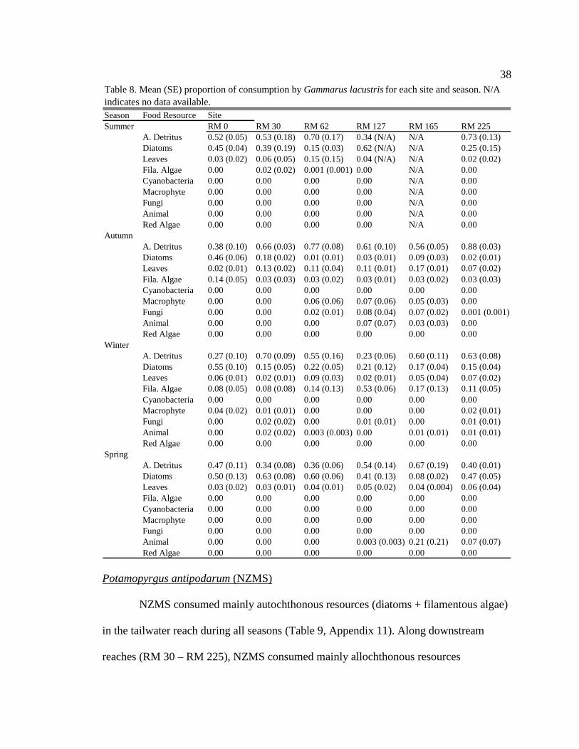
Potamopyrgus antipodarum (NZMS)
NZMS consumed mainly autochthonous resources (diatoms + filamentous algae)
in the tailwater reach during all seasons (Table 9, Appendix 11). Along downstream
reaches (RM 30 – RM 225), NZMS consumed mainly allochthonous resources
39
(amorphous detritus + leaf material) during all seasons (Table 9, Appendix 11). Within
sites there were no consistent seasonal changes in NZMS diets among seasons (Table 9,
Appendix 12), except during moderate turbidity/high light conditions in summer, when
NZMS generally consumed higher proportions of diatoms (though not significant) at
downstream sites.
In the tailwaters, autochthonous organic matter (diatoms + filamentous algae +
autochthonously derived amorphous detritus) contributes the greatest amount to NZMS
production; contributing 98% to the average yearly (average for all four seasons) NZMS
production (Figure 5). At downstream sites, allochthonous organic matter
(allochthonously derived amorphous detritus + leaf material) contributes 55% to the
average yearly (average for all four seasons and all five downstream sites) NZMS
production (Figure 5). Specifically, in the tailwaters, diatoms contribute the greatest
amount to NZMS production during all seasons (72%-84%, range for all seasons) (Table
7). In contrast, at downstream sites, during high turbidity conditions in autumn,
allochthonous amorphous detritus contributes the greatest amount to NZMS production
(41-74%, range for the five downstream sites). During moderate turbidity conditions in
the summer, winter, and spring, diatoms and allochthonous amorphous detritus contribute
somewhat equally to production (Table 7). During these seasons diatoms can contribute
from 18-79% (range for the five downstream sites, during the three moderate turbidity
seasons), and allochthonous amorphous detritus can contribute from 15-77% (range for
the five downstream sites, during the three moderate turbidity seasons) to NZMS
production.
40
Season Food Resource SiteSummer RM 0 RM 30 RM 62 RM 127 RM 165 RM 225
A. Detritus 0.42 (0.07) 0.55 (0.05) 0.89 (N/A) 0.49 (0.04) N/A 0.40 (0.13)Diatoms 0.51 (0.10) 0.30 (0.09) 0.07 (N/A) 0.27 (0.06) N/A 0.56 (0.13)Leaves 0.00 0.15 (0.05) 0.04 (N/A) 0.24 (0.07) N/A 0.04 (0.04)Fila. Algae 0.07 (0.06) 0.00 0.00 0.00 N/A 0.00Cyanobacteria 0.00 0.00 0.00 0.00 N/A 0.00Macrophyte 0.00 0.00 0.00 0.00 N/A 0.00Fungi 0.00 0.00 0.00 0.00 N/A 0.00Animal 0.00 0.00 0.00 0.00 N/A 0.00Red Algae 0.00 0.00 0.00 0.00 N/A 0.00
Autumn A. Detritus 0.39 (0.02) 0.76 (0.04) 0.79 (0.04) 0.76 (0.03) 0.68 (0.05) 0.88 (0.01)Diatoms 0.59 (0.02) 0.18 (0.04) 0.11 (0.03) 0.18 (0.03)0.22 (0.06) 0.08 (0.02)Leaves 0.02 (0.005) 0.06 (0.02) 0.08 (0.01) 0.05 (0.01)0.07 (0.01) 0.04 (0.01)Fila. Algae 0.003 (0.004) 0.00 0.01 (0.004) 0.00 0.01 (0.01) 0.00Cyanobacteria 0.00 0.00 0.00 0.00 0.00 0.00Macrophyte 0.00 0.00 0.00 0.00 0.01 (0.01) 0.00Fungi 0.00 0.00 0.01 (0.01) 0.01 (0.002) 0.01 (0.003) 0.003 (0.003)Animal 0.00 0.00 0.00 0.00 0.00 0.00Red Algae 0.00 0.00 0.00 0.00 0.00 0.00
Winter A. Detritus 0.30 (0.11) 0.52 (0.03) N/A 0.77 (0.05) 0.64 (0.03) 0.43 (0.10)Diatoms 0.65 (0.10) 0.27 (0.05) N/A 0.03 (0.01) 0.15 (0.02) 0.27 (0.14)Leaves 0.01 (0.002) 0.21 (0.03) N/A 0.19 (0.04) 0.21 (0.04) 0.29 (0.04)Fila. Algae 0.01 (0.01) 0.00 N/A 0.00 0.00 0.00Cyanobacteria 0.00 0.00 N/A 0.00 0.00 0.00Macrophyte 0.03 (0.02) 0.00 N/A 0.00 0.00 0.00Fungi 0.00 0.001 (0.001) N/A 0.01 (0.01) 0.00 0.01 (0.005)Animal 0.00 0.00 N/A 0.00 0.00 0.00Red Algae 0.00 0.00 N/A 0.00 0.00 0.00
Spring A. Detritus 0.33 (0.08) 0.78 (0.03) 0.82 (0.05) 0.72 (0.03) 0.77 (0.07) 0.72 (0.11)Diatoms 0.64 (0.08) 0.18 (0.04) 0.13 (0.05) 0.21 (0.04)0.11 (0.04) 0.11 (0.05)Leaves 0.03 (0.01) 0.04 (0.01) 0.04 (0.01) 0.07 (0.03) 0.12 (0.04) 0.14 (0.07)Fila. Algae 0.00 0.00 0.00 0.00 0.00 0.03 (0.03)Cyanobacteria 0.00 0.00 0.00 0.00 0.00 0.00Macrophyte 0.00 0.00 0.01 (0.01) 0.00 0.00 0.00Fungi 0.00 0.00 0.00 0.00 0.00 0.00Animal 0.00 0.00 0.00 0.00 0.00 0.00Red Algae 0.00 0.00 0.00 0.00 0.00 0.00
Table 9. Mean (SE) proportion of consumption by Potamopyrgus antipodarum(NZMS) for each site and season. N/A indicates no data available.
Chironomidae
Chironomids predominately consumed autochthonous resources (diatoms +
filamentous algae) in the tailwater reach (RM 0) during all seasons (Table 10, Appendix
13). Along downstream reaches (RM 30 – RM 225), chironomids consumed mainly
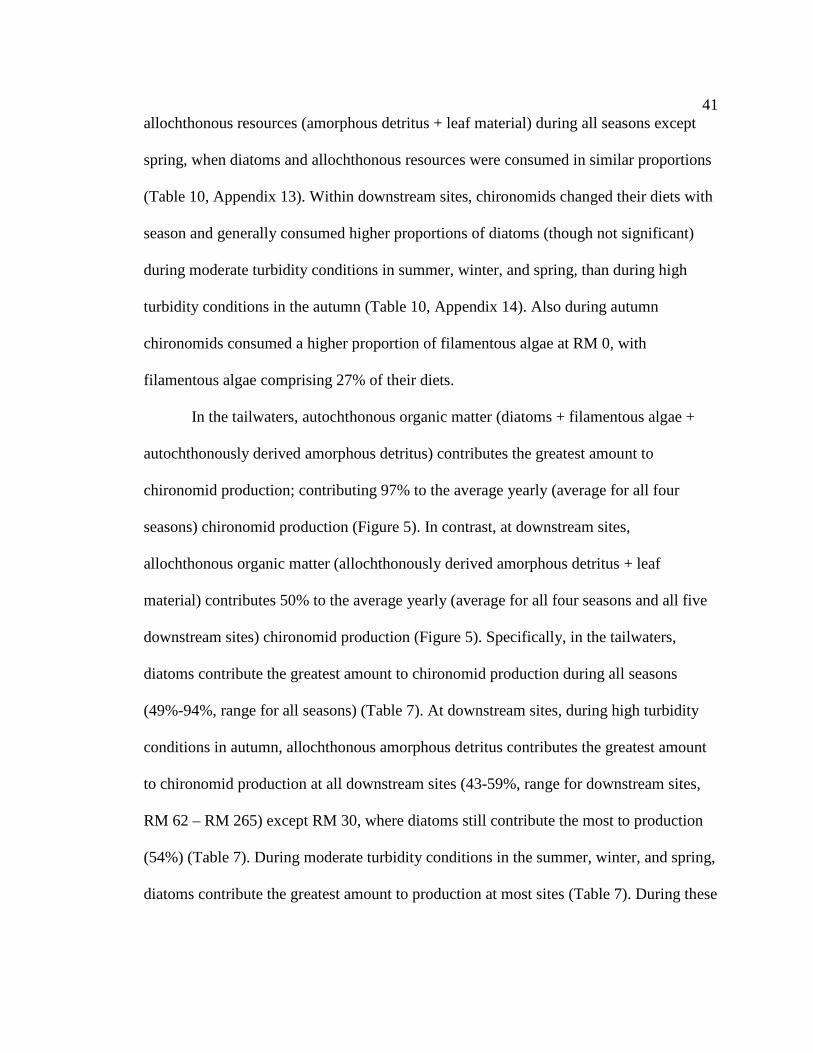
41
allochthonous resources (amorphous detritus + leaf material) during all seasons except
spring, when diatoms and allochthonous resources were consumed in similar proportions
(Table 10, Appendix 13). Within downstream sites, chironomids changed their diets with
season and generally consumed higher proportions of diatoms (though not significant)
during moderate turbidity conditions in summer, winter, and spring, than during high
turbidity conditions in the autumn (Table 10, Appendix 14). Also during autumn
chironomids consumed a higher proportion of filamentous algae at RM 0, with
filamentous algae comprising 27% of their diets.
In the tailwaters, autochthonous organic matter (diatoms + filamentous algae +
autochthonously derived amorphous detritus) contributes the greatest amount to
chironomid production; contributing 97% to the average yearly (average for all four
seasons) chironomid production (Figure 5). In contrast, at downstream sites,
allochthonous organic matter (allochthonously derived amorphous detritus + leaf
material) contributes 50% to the average yearly (average for all four seasons and all five
downstream sites) chironomid production (Figure 5). Specifically, in the tailwaters,
diatoms contribute the greatest amount to chironomid production during all seasons
(49%-94%, range for all seasons) (Table 7). At downstream sites, during high turbidity
conditions in autumn, allochthonous amorphous detritus contributes the greatest amount
to chironomid production at all downstream sites (43-59%, range for downstream sites,
RM 62 – RM 265) except RM 30, where diatoms still contribute the most to production
(54%) (Table 7). During moderate turbidity conditions in the summer, winter, and spring,
diatoms contribute the greatest amount to production at most sites (Table 7). During these
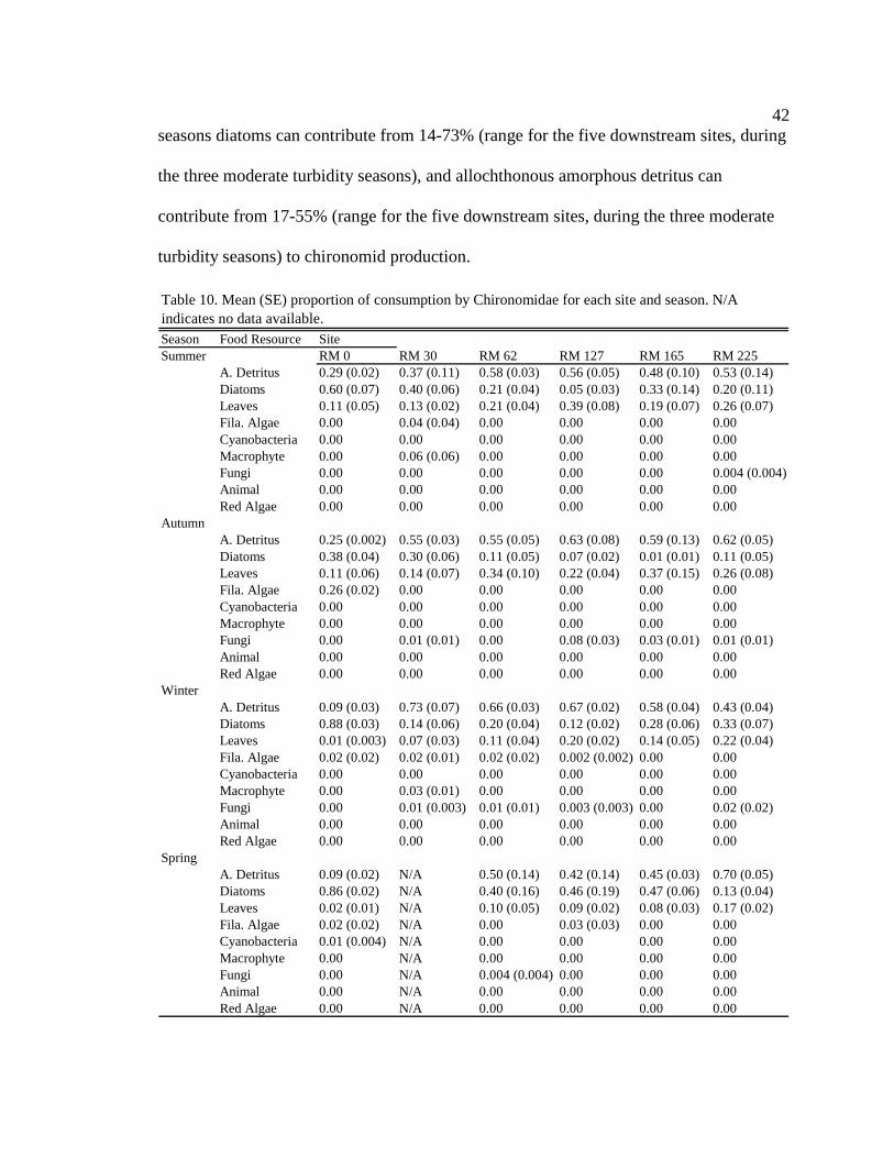
42
seasons diatoms can contribute from 14-73% (range for the five downstream sites, during
the three moderate turbidity seasons), and allochthonous amorphous detritus can
contribute from 17-55% (range for the five downstream sites, during the three moderate
turbidity seasons) to chironomid production.
Season Food Resource SiteSummer RM 0 RM 30 RM 62 RM 127 RM 165 RM 225
A. Detritus 0.29 (0.02) 0.37 (0.11) 0.58 (0.03)0.56 (0.05) 0.48 (0.10) 0.53 (0.14)Diatoms 0.60 (0.07) 0.40 (0.06) 0.21 (0.04) 0.05 (0.03)0.33 (0.14) 0.20 (0.11)Leaves 0.11 (0.05) 0.13 (0.02) 0.21 (0.04) 0.39 (0.08) 0.19 (0.07) 0.26 (0.07)Fila. Algae 0.00 0.04 (0.04) 0.00 0.00 0.00 0.00Cyanobacteria 0.00 0.00 0.00 0.00 0.00 0.00Macrophyte 0.00 0.06 (0.06) 0.00 0.00 0.00 0.00Fungi 0.00 0.00 0.00 0.00 0.00 0.004 (0.004)Animal 0.00 0.00 0.00 0.00 0.00 0.00Red Algae 0.00 0.00 0.00 0.00 0.00 0.00
Autumn A. Detritus 0.25 (0.002) 0.55 (0.03) 0.55 (0.05) 0.63 (0.08) 0.59 (0.13) 0.62 (0.05)Diatoms 0.38 (0.04) 0.30 (0.06) 0.11 (0.05) 0.07 (0.02)0.01 (0.01) 0.11 (0.05)Leaves 0.11 (0.06) 0.14 (0.07) 0.34 (0.10) 0.22 (0.04) 0.37 (0.15) 0.26 (0.08)Fila. Algae 0.26 (0.02) 0.00 0.00 0.00 0.00 0.00Cyanobacteria 0.00 0.00 0.00 0.00 0.00 0.00Macrophyte 0.00 0.00 0.00 0.00 0.00 0.00Fungi 0.00 0.01 (0.01) 0.00 0.08 (0.03) 0.03 (0.01) 0.01 (0.01)Animal 0.00 0.00 0.00 0.00 0.00 0.00Red Algae 0.00 0.00 0.00 0.00 0.00 0.00
Winter A. Detritus 0.09 (0.03) 0.73 (0.07) 0.66 (0.03) 0.67 (0.02) 0.58 (0.04) 0.43 (0.04)Diatoms 0.88 (0.03) 0.14 (0.06) 0.20 (0.04) 0.12 (0.02)0.28 (0.06) 0.33 (0.07)Leaves 0.01 (0.003) 0.07 (0.03) 0.11 (0.04) 0.20 (0.02)0.14 (0.05) 0.22 (0.04)Fila. Algae 0.02 (0.02) 0.02 (0.01) 0.02 (0.02) 0.002 (0.002) 0.00 0.00Cyanobacteria 0.00 0.00 0.00 0.00 0.00 0.00Macrophyte 0.00 0.03 (0.01) 0.00 0.00 0.00 0.00Fungi 0.00 0.01 (0.003) 0.01 (0.01) 0.003 (0.003) 0.00 0.02 (0.02)Animal 0.00 0.00 0.00 0.00 0.00 0.00Red Algae 0.00 0.00 0.00 0.00 0.00 0.00
Spring A. Detritus 0.09 (0.02) N/A 0.50 (0.14) 0.42 (0.14) 0.45 (0.03) 0.70 (0.05)Diatoms 0.86 (0.02) N/A 0.40 (0.16) 0.46 (0.19) 0.47 (0.06) 0.13 (0.04)Leaves 0.02 (0.01) N/A 0.10 (0.05) 0.09 (0.02) 0.08 (0.03) 0.17 (0.02)Fila. Algae 0.02 (0.02) N/A 0.00 0.03 (0.03) 0.00 0.00Cyanobacteria 0.01 (0.004) N/A 0.00 0.00 0.00 0.00Macrophyte 0.00 N/A 0.00 0.00 0.00 0.00Fungi 0.00 N/A 0.004 (0.004) 0.00 0.00 0.00Animal 0.00 N/A 0.00 0.00 0.00 0.00Red Algae 0.00 N/A 0.00 0.00 0.00 0.00
Table 10. Mean (SE) proportion of consumption by Chironomidae for each site and season. N/A indicates no data available.
43
Relative contribution of autochthonous and allochthonous resources to the
macroinvertebrate community
Macroinvertebrate production in the Grand Canyon is supported by
autochthonous resources in the tailwaters (Figure 5, Table 7). In contrast, at downstream
sites, macroinvertebrate production is generally supported by a combination of
autochthonous and allochthonous resources during moderate turbidity conditions (Table
7), and mainly allochthonous resources during high turbidity conditions. Specifically,
during high turbidity conditions allochthonous amorphous detritus contributes the
greatest amount to production at downstream sites, and during moderate turbidity
conditions diatoms and allochthonous amorphous detritus contribute somewhat equally to
production.
Resource consumption relative to resource availability
Resources consumed were generally related to their availability. Composition of
the seston, especially the percentage of diatoms and amorphous detritus, was positively
related to the diets of S. arcticum (r = 0.866, p < 0.001; r =0.610, p = 0.002, respectively,
Figure 6); however, other components of the seston were not related to S. arcticum diets
(Table 11). Epilithic and epicremnic biofilm composition were positively related to each
other (r = 0.853, p < 0.001), so only epilithic biofilms were compared to gut-contents of
G. lacustris, NZMS and chironomids (Figure 6). Consumption of diatoms and amorphous
detritus by these three taxa was positively related to the relative proportion of these
resources in the epilithon (Figure 6). In addition, NZMS consumption of leaf material and
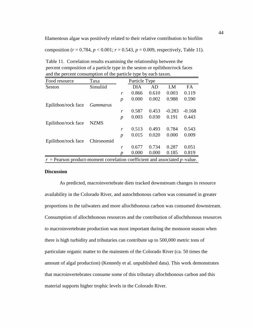
44
filamentous algae was positively related to their relative contribution to biofilm
composition (r = 0.784, p < 0.001; r = 0.543, p = 0.009, respectively, Table 11).
Food resource Taxa Particle TypeSeston Simuliid DIA AD LM FA
r 0.866 0.610 0.003 0.119p 0.000 0.002 0.988 0.590
Epilithon/rock face Gammarusr 0.587 0.453 -0.283 -0.168p 0.003 0.030 0.191 0.443
Epilithon/rock face NZMSr 0.513 0.493 0.784 0.543p 0.015 0.020 0.000 0.009
Epilithon/rock face Chironomidr 0.677 0.734 0.287 0.051p 0.000 0.000 0.185 0.819
Table 11. Correlation results examining the relationship between the percent composition of a particle type in the seston or epilithon/rock faces and the percent consumption of the particle type by each taxon.
r = Pearson product-moment correlation coefficient and associated p -value.
Discussion
As predicted, macroinvertebrate diets tracked downstream changes in resource
availability in the Colorado River, and autochthonous carbon was consumed in greater
proportions in the tailwaters and more allochthonous carbon was consumed downstream.
Consumption of allochthonous resources and the contribution of allochthonous resources
to macroinvertebrate production was most important during the monsoon season when
there is high turbidity and tributaries can contribute up to 500,000 metric tons of
particulate organic matter to the mainstem of the Colorado River (ca. 50 times the
amount of algal production) (Kennedy et al. unpublished data). This work demonstrates
that macroinvertebrates consume some of this tributary allochthonous carbon and this
material supports higher trophic levels in the Colorado River.
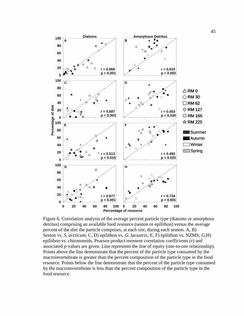
45
0 20 40 60 80 100
r = 0.734 p < 0.001
0 20 40 60 80 1000
20
40
60
80
100
r = 0.677 p < 0.001
G H
r = 0.493 p = 0.020
0
20
40
60
80
100
r = 0.513 p = 0.015
FE
r = 0.453 p = 0.030
0
20
40
60
80
100
r = 0.587 p = 0.003
C D
Diatoms
0
20
40
60
80
100
r = 0.866 p < 0.001
Amorphous Detritus
r = 0.610 p = 0.002
A B
Percentage of resource
Per
cen
tag
e o
f d
iet
Figure 6. Correlation analysis of the average percent particle type (diatoms or amorphous detritus) comprising an available food resource (seston or epilithon) versus the average percent of the diet the particle comprises, at each site, during each season. A, B) Seston vs. S. arcticum; C, D) epilithon vs. G. lacustris; E, F) epilithon vs. NZMS; G,H) epilithon vs. chironomids. Pearson product-moment correlation coefficients (r) and associated p-values are given. Line represents the line of equity (one-to-one relationship). Points above the line demonstrate that the percent of the particle type consumed by the macroinvertebrate is greater than the percent composition of the particle type in the food resource. Points below the line demonstrate that the percent of the particle type consumed by the macroinvertebrate is less than the percent composition of the particle type in the food resource.
RM 0
RM 62
RM 127
RM 165
RM 225
RM 30
RM 0RM 0
RM 62RM 62
RM 127RM 127
RM 165RM 165
RM 225RM 225
RM 30RM 30
Summer
Autumn
Winter
Spring
Summer
Autumn
Winter
Spring
46
Shifts in resource availability and macroinvertebrate consumption
Seston
Composition of the seston displayed the strongest patterns among resources in
spatial and seasonal shifts in composition and shifted most drastically between the
tailwaters (RM 0) and downstream sites (RM 30 – RM 225) during high turbidity and
low light conditions. The flooding of two major tributaries, the Paria River (RM 1.0) and
the Little Colorado River (RM 61) contribute the largest amounts of suspended sediment
and organic matter to the mainstem and consequently amorphous detritus and leaf
material dominate seston community composition downstream of these tributaries.
Previous analyses of seston from the Paria River using stable isotopes indicate derivation
from upland and riparian vegetation, and the isotopic signature was distinct from seston
in the mainstem Colorado River tailwaters (Angradi 1994). During seasons when there
are significant tributary inputs, amorphous detritus in the seston is most likely
allochthonous in origin. During moderate turbidity and high light seasons when there is
higher primary production in the tailwaters and downstream, the downstream shift from
diatoms to amorphous detritus and leaf material is less drastic. In addition, during these
seasons amorphous detritus may be a combination of autochthonously-derived material
exported from the tailwaters, and autochthonously- and allochthonously-derived material
from tributaries. The Paria River is generally turbid, but many smaller tributaries are
clear and may contribute both autochthonous and allochthonous material to the mainstem.
47
Epilithic biofilms
Although, autochthonous resources dominated the composition of epilithic
biofilms in the tailwaters, and allochthonous resources dominated the composition
downstream, there were few significant differences in the proportion of particle types in
the tailwaters versus downstream sites. Filamentous algae significantly declined at
downstream sites during the summer and winter; however, due to high variability among
replicates, no significant patterns in the spatial distribution of diatom composition were
discerned during any season. Monsoon flooding increases the concentration of suspended
sediments and turbidity in the river and reduces water clarity, light levels and gross
primary production (Yard et al. 2003), but does not typically scour or disturb the benthos.
The reduction of peak discharges due to the Glen Canyon Dam has led to increased
substrate stability (Webb et al. 1999, 2005), which allows for significant periphyton
development. Diatom communities, particularly late-successional species typical of well-
developed periphyton communities, are often adapted to survive in low light conditions
(McCormick and Stevenson 1991, Tuji 2000, Sigee 2005) and community composition
may not change considerably at downstream sites, even when light levels are reduced. In
contrast, the dominant filamentous algae in this system, Cladophora glomerata grows
best at high light intensities (McMillan and Verduin 1953, Whitton 1967), and the sharp
decline in its distribution downstream may be attributed to low light levels. Furthermore,
canyon orientation and topographic complexity leads to temporal and spatial solar
insolation and may contribute to high variability in epilithic community composition
(Yard et al. 2005). Finally, there was often more amorphous detritus and leaf material on
48
rocks from downstream sites, which may be attributed to settling and deposition of
tributary and riparian allochthonous material.
Epicremnic biofilms
Epicremnic biofilms were generally similar to epilithic biofilms. Tailwater
epicremnic biofilms were dominated by autochthonous resources during all seasons
except winter, and downstream sites were dominated by allochthonous resources at all
sites, except during high light and moderate turbidity conditions in the spring and
summer, when autochthonous resources were higher. Unlike epilithic biofilms,
significant differences in the proportion of particle types in the tailwaters versus
downstream sites were more prevalent, particularly during high light conditions in the
summer and high turbidity conditions in the autumn. Differences between epilithic and
epicremnic biofilms may be due to differences in sampling methods (rocks were grabbed
out of rivers and scrubbed in a bucket, cliffs were scrubbed in the river with a
scrubbing/sucking device), or different current velocities and depths. Rocks were
typically grabbed from high velocity cobble bars and may not retain allochthonous
material. Cliff faces are adjacent to deep low-velocity areas, which promotes
development of thicker biofilms that may retain more allochthonous material.
Macroinvertebrate diets
Differences among taxa in extent of longitudinal and seasonal diet shifts may be
attributed to differences in food acquisition and availability of resources. As expected,
resource consumption by S. arcticum was highly correlated with seston composition. S.
arcticum is generally classified as a collector-filterer (Cummins 1973), and comparison
49
of their diets to seston community composition, confirms the importance of this food
resource for these filter-feeding organisms (Wallace and Merritt 1980, Wotton 1984,
Parkes et al. 2004). For example, S. arcticum consumption generally matched the
seasonal and longitudinal shifts occurring in the seston and displayed the greatest shift in
diet amongst taxa, shifting diets during all seasons. Site-specific seasonal shifts in S.
arcticum diets were most prevalent at RM 30 and RM 62 (the sites below the two major
tributaries) between the autumn and all other seasons, confirming the effect of tributary
floods on resource availability and consumption. Tributary inputs, particularly during the
autumn, also contributed significantly more leaf material to the seston than was
consumed by S. arcticum. Although, simuliids can ingest particles up to 350 µm (Wotton
1976, Wallace and Merritt 1980, Currie and Craig 1987), the majority of studies report
ingestion of particles less than 100 µm (Wallace and Merritt 1980). The mismatch
between leaf material in the seston and gut contents may be attributed to their inability to
filter larger leaf particles from the seston. In addition, larval ingestion rates (Hart and
Latta 1986, Hart 1987) and densities (Erman and Chouteau 1979, Hart 1987) have been
shown to be positively correlated with food availability. As such, filtering organisms may
benefit from increased seston concentrations leading to higher ingestion rates. The
success of S. arcticum in the Colorado River ecosystem may be due to its ability to
effectively access and exploit changing resources.
G. lacustris diets track available resources and their resource consumption was
significantly correlated with epilithic resource composition. In contrast to S. arcticum, G.
lacustris only shifted diets to consume more allochthonous resources at downstream sites
50
during three of the four seasons, and during spring consumed a higher proportion of
autochthonous resources at most of the downstream sites. Also at downstream sites
during moderate turbidity and moderate/high light conditions in the spring and summer,
G. lacustris consumed higher proportions of diatoms than in the autumn and winter. G.
lacustris are classified as facultative shredders (Cummins and Klug 1979) and because of
their ability to move upstream by swimming and crawling along substrates (Hughes
1970); they are not constrained to feeding in one habitat. The epilithon of the tailwaters
of Glen Canyon Dam is dominated by Cladophora glomerata and this is the preferred
habitat of G. lacustris (Shannon et al. 1994) and epiphytic diatoms are their preferred
food resource (Pinney 1991). G. lacustris are also common on cliff faces, especially
when Cladophora glomerata cover is low in winter and spring (personal observation).
Downstream, G. lacustris is found on cliff faces; root wads associated with undercut
banks; macrophytes and bryophytes; reeds and sedges such as Phragmites australis and
Carex aquatilis; and rarely on cobble bars (personal observation). G. lacustris may be
able to utilize a variety of habitats to selectively feed on preferred resources (Bärlocher
1985, Arsuffi and Suberkropp 1989, Friberg and Jacobsen 1994), which may explain
their higher consumption of autochthonous resources at downstream sites during some
seasons. Specifically, in this system G. lacustris selectively feeds on epiphytic diatoms
(Pinney 1991).
My results show G. lacustris feeds on more amorphous detritus than previously
reported. In the tailwaters, this amorphous detritus is most likely autochthonously derived
because of the lack of upstream allochthonous inputs. In addition, amorphous detritus
51
may be derived from algal exudates (or algal exopolymer secretions) (Hart and Lovvorn
2003) and may be ingested while feeding on epiphytes. Therefore, G. lacustris higher
consumption of autochthonous resources downstream during moderate turbidity and
moderate/high light seasons may be attributed to G. lacustris preference for epiphytic
diatoms and associated detritus. During high turbidity and low light conditions (autumn
and winter), G. lacustris consume more amorphous detritus and leaf material than
diatoms. During these seasons, G. lacustris had a more varied diet and also consumed
macrophytes, fungi, and animal material at downstream sites (although in low
proportions) and this may be because of the lower availability of autochthonous resources
on cliff faces. Furthermore, Gammarus prefer conditioned (high microbial biomass) to
unconditioned leaves (Bärlocher 1985) and, in this system, allochthonous inputs from
tributaries may be a higher quality conditioned resource, due to higher water
temperatures in tributaries. Similar to black flies, G. lacustris is an omnivorous and
opportunistic feeder that is capable of shifting diets.
New Zealand mud snail diets also track changes in epilithon resource availability
and NZMS consumed more autochthonous resources in the tailwaters than downstream
during all seasons. New Zealand mud snails are classified as facultative scraper/grazers
that feed on the periphyton/mucopolysaccharide matrix (an assemblage of diatoms,
filamentous algae, algal exudates/mucilage, amorphous detritus, fungi, bacteria and other
leaf, plant and animal material); therefore, they consume a variety of resources including
diatoms, green algae, and plant and animal detritus (Haynes and Taylor 1984). New
Zealand mud snail resource consumption was correlated with the epilithic resource
52
composition and NZMS were the only taxa correlated with all four of the dominant
particles (diatoms, amorphous detritus, leaf material, and filamentous algae), confirming
the importance of the periphyton matrix as a food resource. New Zealand mud snails
thrive in autochthonously driven systems (Hall et al. 2006), and during summer when
there is the highest availability of autochthonous resources, NZMS generally consumed
more algae at all downstream sites than other seasons. In contrast, when the availability
of autochthonous resources is lower during autumn, winter, and spring, NZMS generally
consumed more amorphous detritus and leaf material at downstream sites. In addition, at
downstream sites NZMS are most common in cobble bars with slow current velocities
(personal observation). New Zealand mud snail preference for habitats with slower water
velocities (Vinson 2004), which facilitate organic matter deposition, may explain the
increase in consumption of allochthonous resources downstream during these seasons.
Although NZMS consume allochthonous resources downstream, secondary production of
NZMS is typically highest in autochthonously driven systems (Hall et al. 2006), and
algae may be a better food resource. The low availability of autochthonous material
downstream, particularly during high turbidity conditions, may explain their low
abundance at downstream sites (Cross et al. unpublished data).
Chironomid diets tracked the availability of epilithic resources. Amongst taxa
feeding on the epilithon, chironomids were the most highly correlated with epilithic
resource composition of the dominant particles, diatoms and amorphous detritus,
demonstrating the importance of epilithic resources for these taxa (Figure 5).
Chironomids generally consumed more allochthonous than autochthonous resources at
53
downstream sites during all seasons, expect in the spring when similar proportions were
consumed. The equal consumption of resources during the spring may be attributed to a
number of factors. Although chironomids are most commonly classified as collector-
gatherers, like other aquatic insects they are opportunistic and omnivorous and use
multiple feeding modes (Berg 1995, Ferrington et al. 2008, Henriques-Oliveira et al.
2003); therefore, chironomids typically rely on a variety of resources. It has been
previously demonstrated that factors such as larval size, sediment composition and food
quality can influence chironomid feeding behavior (McLachlan et al. 1978, Hodkinson
and Williams 1980, Berg 1995). Furthermore, unlike other taxa in this study, there are
multiple species of chironomids present in this system, which may use different feeding
modes, habitats, and food resources. Twenty-four species of chironomids have been
reported in this system (Stevens et al.1998) and four genera (Cricotopus, Orthocladius,
Eukiefferiella, and Tvetenia: subfamily Orthocladiinae), were consistently collected for
gut-content analysis in this study. These chironomids are typically found in a variety of
habitats including rock and cliff faces, depositional zones, and associated with
filamentous algae and other aquatic plants. Diet data of chironomids of all four genera,
found in multiple habitats, were averaged at each site for each season, and therefore may
mask spatial and seasonal diet trends that might exist for individual species. Further
analysis of chironomid diets by size and genus may help elucidate diet shifts.
Shifts in food quality
Food resources in rivers vary in quality (i.e. algae is typically higher quality food
than leaf material); therefore, changes in food resources consumed by macroinvertebrates
54
may influence their growth and production (Benke and Wallace 1980, Bird and Kaushik
1984, Rosi-Marshall and Meyer 2004). Autochthonous carbon (i.e. diatoms and
filamentous algae) is more easily assimilated than allochthonous carbon (i.e. leaf
material) (Benke and Wallace 1997), so in a system with seasonal or spatial changes in
resource availability there may be shifts in macroinvertebrate production due to resource
quality. The quality of allochthonous resources may also vary seasonally and
longitudinally. In particular, higher temperatures in tributaries (seasonally relative to the
mainstem) may increase microbial colonization of allochthonous resources, increasing
the quality of the resource (by adding microbes as a food resource), or decreasing the
quality as microbes consume it and the residual material becomes more recalcitrant
(Short and Smith 1989, Abelho 2001, Graça and Canhoto 2006). Finally, a common food
resource for macroinvertebrates in many large river systems, including the Colorado
River, is amorphous detritus (Benke and Wallace 1997, Rosi-Marshall and Wallace
2002). The source (i.e. autochthonous versus allochthonous) of amorphous detritus may
affect its quality and assimilation efficiency (Rosi-Marshall and Meyer 2004). In the
tailwaters of Glen Canyon Dam, amorphous detritus may be primarily derived from
autochthonous organic matter. In contrast, when primary production is low due to
increased tributary-induced turbidity, amorphous detritus may be primarily derived from
allochthonous organic matter from upland vegetation.
Because of varying assimilability, examining macroinvertebrate diets can cause
misinterpretation of which food resources are actually supporting macroinvertebrate
secondary production. Because autochthonous resources are assimilated more efficiently
55
than amorphous detritus and leaf material, they may contribute substantially to
macroinvertebrate production, even in rivers where algal production and consumption is
lower than allochthonous organic matter inputs and consumption (Thorp and Delong
2002). In the tailwaters of this system, autochthonous resources (predominantly diatoms)
are consumed in higher proportions than allochthonous resources and contribute the
greatest amount to macroinvertebrate production during all seasons. At downstream sites,
amorphous detritus is generally consumed in higher proportions than diatoms; however,
because of diatoms high assimilation efficiency, autochthonous resources still contribute
substantially to macroinvertebrate production (Figure 5), particularly during moderate
turbidity conditions (Table 7). Allochthonous resources (predominantly allochthonous
amorphous detritus) also contribute substantially to downstream macroinvertebrate
production (Table 7), particularly during high turbidity conditions when it dominates the
diets of macroinvertebrates and supports a high percentage (31-93%) of their production,
despite its low assimilability. I calculated the percent of allochthonously and
autochthonously derived amorphous detritus (see methods), and the same assimilation
efficiency, 0.1, was applied to both types of amorphous detritus for production
attributable estimates. As discussed earlier, autochthonously derived amorphous detritus
may be highly assimilable (Hart and Lovvorn 2003), and my calculation of production
attributable to autochthonous resources may be underestimated. In contrast, during high
turbidity conditions, when amorphous detritus is most likely from tributary flooding and
allochthonously derived, the production attributable to allochthonous resources may be
an underestimate. In conclusion, macroinvertebrate production in the tailwaters is
56
supported by autochthonous carbon, and downstream macroinvertebrate production is
supported by a combination of autochthonous and allochthonous resources, during
moderate turbidity conditions, and allochthonous resources during high turbidity
conditions induced by monsoon tributary floods.
Serial discontinuity concept
Dams alter the natural state of rivers, influencing their physical and chemical
properties, and ultimately changing the structure and function of downstream ecosystems
(Baxter 1977, Power et al. 1996, Poff and Hart 2002). Restoration of river systems below
dams can be assessed by examining the recovery of biophysical properties such as
temperature, flow, and species distributions (Ward and Stanford 1983). The river
continuum concept (RCC) predicts that longitudinal changes in physical characteristics of
rivers from the headwaters to the mouth will be accompanied by a corresponding shift in
energy inputs and the structure and function of biological communities (Vannote et al.
1980). The concept predicts that large rivers will be heterotrophic, with a
macroinvertebrate community dominated by collectors because they are efficient
processors of fine particulate organic matter (Vannote et al. 1980). The serial
discontinuity concept (SDC) suggests that dams lead to discontinuities in the longitudinal
characteristics predicted by the RCC, essentially resetting river conditions to that of a
more upstream site. The SDC predicts that ecosystems will recover toward pre-dam
conditions (or conditions predicted by the RCC) with increased distance from the dam
and unregulated tributary inputs (Ward and Stanford 1983, 1995, Stanford and Ward
2001). System recovery has been evaluated by examining variables such as temperature,
57
flow regime, substratum composition, species abundance and diversity, and ratios of
photosynthesis to respiration (Ward and Stanford 1983, Stanford and Ward 2001). The
ability of a system to recover may be influenced by the size and operational mode of the
dam, the longitudinal placement of the dam along the river continuum, the distance
between dams, the size, number and discharge of unregulated tributary inputs, the extent
of longitudinal, lateral and vertical connectivity between the river channel and
floodplains, and biome type (Ward and Stanford 1995, Stanford and Ward 2001).
Some systems downstream of dams may never recover (Stanford and Ward 2001,
Stevens et al. 1997). For example, in Grand Canyon, temperature, discharge and species
diversity do not recover before the river encounters another reservoir (Stanford and Ward
2001, Stevens et al. 1997). Stevens et al. (1997) estimates that recovery of the thermal
regime to pre-dam conditions would require 930 km of river. Hoover dam is only 400 km
downstream of Glen Canyon Dam. The lack of recovery of the thermal regime in this
system may strongly influence the recovery of macroinvertebrate biodiversity.
The Colorado River in Grand Canyon does not recover its thermal regime (i.e.
there is little downstream warming (Wright et al. 2009)). However, my data demonstrate
that macroinvertebrates consume tributary allochthonous carbon delivered to the
mainstem, which may be similar to pre-dam conditions. The “recovery” of this pre-dam
condition of reliance on tributary carbon is a novel metric for ecosystem recovery
downstream of a dam not previously considered in the SDC. This finding suggests that
there may be the potential for recovery of the food web dynamics (and possible
58
concomitant increases in diversity), if other aspects of the river were restored (i.e. thermal
or flow regime).
Conclusion
The aim of this study was to examine how macroinvertebrates diets vary spatially
and temporally in the Colorado River downstream of Glen Canyon Dam. My data
demonstrate that tributary-derived allochthonous carbon and locally produced
autochthonous carbon are important food resources for downstream macroinvertebrates.
The macroinvertebrates in this system are generally opportunistic, facultative feeders, and
their diets reflect changes in organic matter availability. S. arcticum is the most common
macroinvertebrate taxon in sites downstream of the tailwaters, perhaps due to their ability
to consume allochthonous tributary carbon. Macroinvertebrate groups such as filter-
feeders may recover to pre-dam conditions if thermal and flow regimes were restored,
even if organic matter inputs from upstream were not restored, because they may be able
to effectively utilize tributary allochthonous inputs as a food resource.
Currently, more than 42,000 large dams obstruct rivers throughout the world
(ICOLD 1998). The United States contains over 5,000 large dams and ranks second only
to China in terms of the number of large dams (Benke 1990, ICOLD 1998). While these
dams provide a source of water and energy, they also alter the physical habitat,
temperature and flow regime of rivers and contribute significantly to the degradation of
our freshwater ecosystems (Baxter 1977, Ward and Stanford 1979, Petts 1984, Nilsson
and Berggren 2000). The decrease in the biotic integrity of rivers associated with large
dams has led to the extinction and endangerment of over two-fifths of freshwater fishes in
59
the U.S. (McCully 1996). Given that removal of large dams is not usually an option
(Whitelaw and MacMullan 2002, Hart et al. 2002), effective management of dams is
essential to protect biotic integrity. Understanding which resources support food webs
may help to better manage dam operations to increase macroinvertebrate production and
even diversity and may ultimately aid in fish conservation. This research provides
evidence that macroinvertebrates in dammed systems are capable of shifting diets to
access changing resources. However, although the availability of food resources in
dammed systems may recover toward pre-dam conditions due to tributaries, the
macroinvertebrate diversity and production may not recover without the restoration of
physical characteristics (i.e. water temperature and flow regime).
60
CHAPTER TWO
EXPLORING A POTENTIAL PRODUCTIVITY SUBSIDY USING A NOVEL
TRACER IN THE COLORADO RIVER BELOW GLEN CANYON DAM
Abstract
In this study I examined algal taxonomic content of epilithon, epicremnon, seston,
and macroinvertebrate diet at six sites in the Colorado River downstream of Glen Canyon
Dam to address whether primary production in the tailwaters may serve as a resource
subsidy to macroinvertebrates downstream. To address this I attempted to identify algal
species to use as novel tracers, to examine if algal cells produced in tailwaters were used
as a resource by macroinvertebrates downstream. In addition, one indicator species
(Fragilaria crotonensis Kitton) was used to assess algal transport and survival, helping to
further address the potential for tailwater production to support downstream
macroinvertebrates. Tailwater algal assemblages consistently differed from downstream
assemblages, allowing a list of species that could serve as potential indicators for the
tailwater and downstream sites to be identified. Although many of the species were not
common in the system, their specificity to tailwater or downstream sites made them
useful indicators, and helped to identify the origin of macroinvertebrate food resources. I
concluded that macroinvertebrates residing in reaches of the Colorado River well
downstream of Glen Canyon Dam consume a combination of tailwater and downstream
61
(site-specific or tributary species) algae, but tailwater primary production does not solely
fuel downstream macroinvertebrates, and may not serve as an important resource
subsidy. Algal indicators were useful subsidy tracers in this system, and this method may
be useful for addressing food web subsidy questions in other systems.
Introduction
In aquatic ecosystems the importance of resource subsidies from adjacent habitats
and ecosystems has been well documented (Ward 1989, Bilby et al. 1996, Polis et al.
1997, Nakano et al. 1999). A basic tenet in stream ecology is that upstream and
downstream ecosystems are linked via the transport of nutrients and organic matter
(Vannote et al. 1980); therefore, upstream habitats can provide resource subsidies to
downstream food webs. Although the transport of resources from upstream reaches to
downstream ecosystems has been well documented (Fisher and Likens 1973, Angradi
1991, Cushing et al. 1993, Webster et al. 1999, Wipfli et al. 2007), the extent to which
these resources are exploited or subsidize downstream food webs is less understood and
still requires further research (Wipfli et al. 2007).
Recently, food web studies in stream ecosystems have focused on examining the
potential importance of the exchange of resources between the stream and riparian zone
(Nakano and Murakami 2001, Power 2001, Baxter et al. 2005). In large rivers,
particularly in dammed systems, downstream food webs can also be subsidized by
resources from lakes and reservoirs (Petts 1984, Doi et al. 2008, Mercado-Silva et al.
2008); however, the importance of the subsidy may decline as distance from the reservoir
increases (Ward 1975, Doi et al. 2008, Mercado-Silva et al. 2008). Similar to reservoir
62
subsidies, the productive tailwaters downstream of dams may also provide a resource
subsidy to downstream ecosystems. For example, in the Colorado River, the completion
of Glen Canyon Dam in 1963 substantially reduced sediment loads in the river,
increasing light levels and algal production in the tailwaters below the dam (Stevens et al.
1997). Food web analyses in this system have focused on the importance of tailwater-
produced autochthonous resources for macroinvertebrates (Pinney 1991, Shannon et al.
1994) and it has been suggested that the highly productive tailwater below Glen Canyon
Dam may be a resource subsidy to downstream food webs (Blinn et al. 1994, Walters et
al. 2000). However, downstream food webs may also be fueled by local primary
production and inputs of organic matter from tributaries. Tributary flooding contributes
approximately 500,000 metric tons of particulate organic matter to the mainstem of the
Colorado River annually (ca. 50 times the amount of algal production) (Kennedy et al.
unpublished data) and evidence indicates that this organic matter is exploited by
macroinvertebrates and fish downstream of tributary confluences (Angradi 1994, Blinn et
al. 1998, Wellard Kelly (Chapter 1), Zahn et al. unpublished data). Furthermore,
epiphytic diatoms on Cladophora glomerata (L.) Kütz., the dominant filamentous alga in
the tailwaters, have been shown to be heavily exploited by macroinvertebrates in the
tailwaters (Pinney 1991, Stevens et al. 1997). Downstream of the tailwaters, C. glomerata
densities decline significantly (Carothers and Brown 1991). The extent to which
autochthonous production in the tailwaters of Glen Canyon Dam subsidizes food webs
downstream is not currently known. Data presented in Chapter 1 suggest that, during
63
monsoons especially, downstream macroinvertebrates consume allochthonous resources.
However, during seasons with lower turbidity, it is not clear if the algae present in
macroinvertebrate diets is a resource subsidy from the tailwater or if these autochthonous
resources are produced in situ at downstream sites.
To resolve this issue, I used algal taxa with distributions limited to specific river
reaches as tracers, to examine if food resources from one area were exploited by primary
consumers in another. Tracers have proven useful for addressing a number of important
ecological questions. For example, otolith microchemistry has been used to track
migration patterns and habitat use of fishes (Ingram and Weber 1999, Secor et al. 1995,
Clarke et al. 2007). Trace elements can help to identify the source, distribution and
accumulation of pollutants in a variety of ecosystems (Rizzutto et al. 2006, Barber et al.
2006). Detection and dispersion of larvae of invasive invertebrate larvae in aquatic
systems has been accomplished using molecular-genetic markers (Harvey et al. 2009),
Transport length and uptake of particles in streams has been documented using radio-
labeled and fluorescently labeled particles (Cushing et al. 1993, Hall et al. 1996, Thomas
et al. 2001, Newbold et al. 2005), and stable isotopes allow resource use and energy flow
through food webs to be tracked (Hamilton et al. 1992, Peterson 1999). Stable-carbon
isotopes (13C/12C) are the typical tracers used in food web studies to distinguish which
basal resources are utilized by consumers (Rounick et al. 1982, Hamilton et al. 1992,
Rosenfeld and Roff 1992, Bastow et al. 2002), because terrestrial and aquatic plants often
differ in their δ 13C signature (Rounick and Winterbourn 1986). In addition, natural
variation in algal δ 13C, attributed to differences in current velocity or algal productivity
64
(Peterson et al. 1993, Finlay et al. 1999), can also help to spatially differentiate between
utilization of algae produced in different habitats (Finlay et al. 1999).
Although, stable isotopes can be useful for elucidating spatial patterns in algal
resource use in some systems (Finlay et al. 1999), algal δ 13C may be less useful in
systems where δ 13C signatures do not significantly differ among sites (France 1996) or if
there is great variability in algal δ 13C signatures (France 1995a). In particular,
identification of the basal resources used by consumers can be difficult when there is not
sufficient separation or characterization of dietary end-members (Hamilton and Lewis
1992). For example, many aquatic consumers feed on fine particulate organic matter
(FPOM), a mixture of live algae, and detritus derived from algae, consumer feces, or
terrestrial and aquatic plants (Hamilton and Lewis 1992). Therefore, without isotopic
separation of algal and detrital material it may be difficult to determine the importance of
the different basal resources (Hamilton and Lewis 1992). These difficulties demonstrate
that other tracers may be useful to address more specific questions in trophic subsidy
studies.
A novel tracer may be particularly useful to examine if primary production in the
tailwaters is being exploited downstream, because the tailwater and downstream
ecosystems may support algal communities that differ in taxonomic content (Czarnecki
and Blinn, 1978). In particular, community assemblages in the tailwaters may differ from
downstream communities due to physical and chemical changes induced by tributary
inputs. The serial discontinuity concept (SDC) predicts that tributaries downstream of
dams may ameliorate some of the physicochemical condition changes induced by dams
65
(Ward and Stanford 1983, Stevens et al. 1997), inducing differences between tailwater
and downstream communities (Takao et al. 2008). Tributary inputs to the Colorado River
contribute high amounts of suspended sediment and organic matter, resulting in reduced
light levels and concomitant reductions in algal production (Yard 2003, Hall et al.
unpublished data). Furthermore, water temperature in the Colorado River increases with
distance from Glen Canyon Dam (2-10 ◦C) (Wright et al. 2009), a change that has been
shown to influence the species composition, growth, production and distribution of
aquatic communities (Vannote and Sweeney 1980, Blinn et al. 1989, Vinson and
Hawkins 1998, Arscott et al. 2001, Dallas 2008).
Changes in the physical and chemical characteristics of the Colorado River
induced by tributary inputs may lead to changes in the algal community assemblage in
the river (Czarnecki and Blinn, 1978). Algal communities, specifically diatoms, are
important indicators of change in aquatic ecosystems (Dixit et al. 1992, McCormick and
Cairns 1994, Pan et al. 1996), and are useful for water-quality biomonitoring (Reavie and
Smol 1998, Rott et al. 1998, Stevenson and Pan 1999). The structure of benthic algal
communities can be affected by suspended sediment levels, light conditions, temperature,
water chemistry, herbivory, flow conditions and disturbance (Peterson 1987, Blinn et al.
1989, McCormick and Stevenson 1989, Hardwick et al. 1992, Pan and Lowe 1994, Pan et
al. 1996). Because algal communities reflect environmental conditions and respond
quickly to physical, chemical and biological changes, both communities and individual
species may be used as taxonomic indicators of environmental and habitat conditions in
rivers (Dixit et al. 1992, McCormick and Cairns 1994). Rare taxa or specialists (species
66
that have narrow optima and tolerances to certain environmental variables (Dixit et al.
1992, Enache and Prairie 2002, Pither and Aarssen 2005)) may be useful indicators
because they may reflect specific environmental habitat or site conditions.
In the Colorado River, if longitudinal variation in algal species composition
occurs, it may allow for certain species to be used as tracers. Algae are an important food
resource for macroinvertebrates throughout the system (Wellard Kelly (Chapter 1) and
algal tracers may elucidate whether macroinvertebrates along the length of the river rely
on algal production generated locally or on algae produced in the tailwaters of Glen
Canyon Dam and transported downstream (Figures 7 & 8). Similarly, if algal
assemblages in tributaries differ in taxonomic structure from those in the mainstem
(Czarnecki et al. 1976), tributary species representation in macroinvertebrate diets would
also demonstrate the role of tributary inputs of autochthonous production to
macroinvertebrates in the Colorado River food web.
The objective of this study was to determine if species-level identification of
algae can be used to elucidate whether macroinvertebrates rely on upstream food
resources versus site-specific/downstream food resources. Examination and comparison
of the algal communities comprising the epilithon (rock/cobble), epicremnon (cliff/talus),
seston, and macroinvertebrate diets, at six sites over the 226 mile stretch of the river was
used to assess the extent to which tailwaters provide a trophic subsidy to
macroinvertebrate communities downriver.
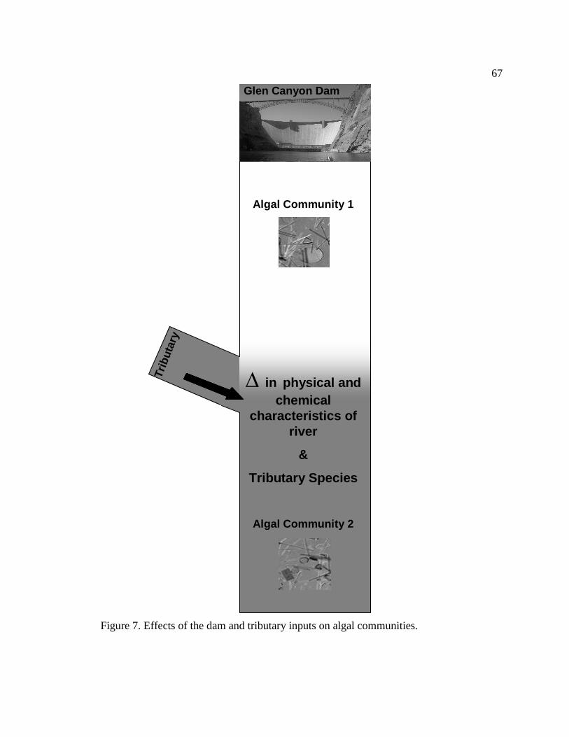
67
Trib
utar
y
Glen Canyon Dam
∆ in physical and chemical
characteristics of river
&
Tributary Species
Algal Community 1
Algal Community 2
Figure 7. Effects of the dam and tributary inputs on algal communities.
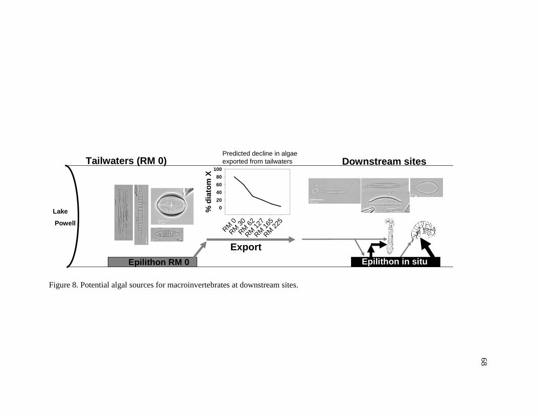
68
Figure 8. Potential algal sources for macroinvertebrates at downstream sites.
RM 0
RM 3
0RM
62
RM 1
27RM
165
RM 2
25
% d
iato
m X
0
20
40
60
80
100Tailwaters (RM 0)
Export
Epilithon RM 0 Epilithon in situ
Downstream sites
Lake
Powell
Predicted decline in algae exported from tailwaters
69
The research question addressed in this study was: Can species-level
identification of algae elucidate highly site-specific feeding versus reliance on tailwater
food resources, and more specifically: 1) Does algae from the tailwaters move/survive
downstream?; 2) Are there species which may be useful indicators for the tailwaters
versus downstream sites?; 3) Do macroinvertebrates downstream of the tailwaters
consume indicator species that originate from the tailwaters?; 4) Do macroinvertebrates
downstream of the tailwaters consume indicator species that originate from downstream
sites?
I predict the identity of algal species consumed by macroinvertebrates will shift in
conjunction with longitudinal changes in the taxonomic content of algal assemblages in
the river (Hardwick et al. 1992). In addition, I predict that algal species will be useful
indicators and will help to examine the importance of upstream and site-specific
resources for macroinvertebrates. I also predict that tailwater algae will be able to
move/survive downstream, although in low numbers, and that downstream
macroinvertebrates will eat mostly downstream diatoms with limited amounts of tailwater
diatoms.
Methods
Study sites and sampling protocol
This study was conducted in the Colorado River (CR) in Grand Canyon, Arizona
(36° 03'N, 112° 09' W). Six sites were sampled over a 226 mile (363 km) reach
downstream of Glen Canyon Dam (GCD) (Figure 2). Sites were selected based on
general canyon characteristics, the location of major tributary inputs, prevalence of
70
humpback chub populations (RM 62 and 127), and based on their long-term use as
sediment and geomorphology monitoring sites (RM 30, 62 and 127). The first site, Lee’s
Ferry (RM 0) is located in Glen Canyon and encompasses a 15.7 mile (25 km) reach
extending from the downstream end of the Glen Canyon Dam to Lee’s Ferry. This
tailwater reach is above the confluence of the Paria River, and is consistently low in
turbidity. The five downstream sites are located in the Grand Canyon, from Marble
Canyon to Diamond Creek. The second site, RM 30, is located in the Marble Canyon
section (Redwall gorge reach) of the Grand Canyon, approximately 29 miles downstream
of the Paria River, the first major tributary below the dam. The third site, RM 62, is
located in the beginning of the Central Grand Canyon section (Furnace flats reach) below
the Little Colorado River (LCR), the largest tributary. The fourth site, RM 127, is also
located in the Central Grand Canyon section (Middle granite gorge reach) below a
number of smaller tributaries including Bright Angel, Shinumo and Fossil Creeks. The
fifth site, RM 165, is located in the Western Grand Canyon section (Lower canyon reach)
below Tapeats, Kanab and Havasu Creeks. The final site, RM 225, is also located in the
Western Grand Canyon section (Lower granite gorge) and extends to Diamond Creek (a
small tributary). Sites, RM 30 and 62, are located in wider sections of the canyon and
sites, RM 127 and 165, are within the narrowest canyon sections (Stevens et al. 1997).
Algal assemblage analysis
The taxonomic structure of algal assemblages were quantified from seston,
epilithic (rock/cobble faces), and epicremnic (cliff faces) samples at each of the six
collection sites during January 2007. These results were compared to algae within the
71
guts of Simulium arcticum and Gammarus lacustris collected from the same sites, during
January 2007, to assess whether macroinvertebrates rely on upstream resources
(produced in the tailwater reach below Glen Canyon) or site specific downstream
resources. In addition, separating out algal communities from seston, epilithic and
epicremnic habitats allowed for assessment of specific locations of macroinvertebrate
feeding activity.
Resource and macroinvertebrate collection
Suspended fine particulate organic matter (seston) composition samples (two to
three per site and date) were collected from the thalweg at each site by sieving river water
through a 250-µm sieve and filtering ca. 40-300 ml onto 0.45-µm grided Metricel®
membrane filters (Pall Corp., Ann Arbor, MI). Epilithic biofilms were scraped from two
to three rocks collected from the river bed and from two to three cliff faces, using a
scraping sucking device. A 30-40 ml subsample of biofilm slurry from individual rocks
and cliffs was preserved in the field with Lugol’s solution (Prescott 1978).
Macroinvertebrates were haphazardly collected throughout the reaches of the six sites,
preserved in Kahle’s solution (Stehr 1987) in the field, and returned to the lab for gut-
content analysis.
Resource composition slide preparation
To examine the taxonomic structure of algal assemblages available for
macroinvertebrate consumption, I quantified the relative abundances of algal species
collected from the seston and epilithic and epicremnic biofilms. For epilithic and
epicremnic biofilms, I filtered 0.1-5.0 ml subsamples from preserved field collections
72
onto 0.45 µm gridded Metricel® membrane filters (Pall Corp., Ann Arbor, MI). Seston,
epilithic and epicremnic filters were mounted on slides for preservation using Type B
immersion oil for subsequent enumeration. Two to three slides were analyzed as
replicates for each habitat at each site.
Macroinvertebrate slide prepartion
Gut-content analysis (Rosi-Marshall and Wallace 2002) was used to examine the
taxonomic structure of algal assemblages in the diets of Simulium arcticum (Insecta:
Diptera: Simuliidae) and Gammarus lacustris (Crustacea: Amphipoda: Gammaridae.
Simulium arcticum was selected for algal assemblage analysis because they are filter-
feeders and their diets may reflect algae that are transported in the water column. G.
lacustris was selected because they are shredders that feed on the benthos and prefer
epiphytic diatoms in this system (Pinney 1991); therefore, their diets may indicate the
transport and deposition of algae from upstream sites. Dissected gut contents were drawn
onto (25mm, 0.45µm) gridded Metricel® membrane filters (Pall Corp., Ann Arbor, MI)
and mounted on slides for preservation using Type B immersion oil. I used guts from one
to four individual macroinvertebrates for each slide. Two to three slides were analyzed
for each taxon at each site.
Microscopy
Algal species were identified at 1000x magnification using an Olympus BX50 or
BH2 microscope equipped with a camera for image analysis. The following taxonomic
references were used for identifications: Czarnecki and Blinn (1977), Czarnecki and
Blinn (1978), Patrick and Reimer (1966), Patrick and Reimer (1975). At least 300 valves
73
were identified from each slide or ten full transects were scanned, which ever occurred
first. During identification each valve was recorded as live or dead by examining intact
chloroplasts. All calculations included both live and dead cells unless otherwise noted.
One to three slides were analyzed for each habitat (seston, epilithon and epicremnon) at
each site, and gut contents were quantified from two to three slides for each
macroinvertebrate taxon at each site. The relative abundance of individual algal species
was calculated for each sample and used to calculate the mean relative abundance of each
algal species at each site, for each habitat and macroinvertebrate taxa.
Algal movement and survival
To address whether algae from the tailwaters are transported and survive
downstream, Fragilaria crotonensis Kitton, a dominant planktonic diatom in Lake
Powell and its tailwaters, was selected from seston samples to serve as a tracer for
autochthonous tailwater production. The total number of live versus dead F. crotonensis
cells per milliliter of filtered seston was compared across all sites, to assess the potential
for tailwater algae to move and survive downstream and be consumed by
macroinvertebrates. The relative contribution of F. crotonensis to the total number of
cells in a seston sample was calculated to compare to the proportions measured in
macroinvertebrate diets.
Algal transport distance and deposition velocity
To estimate longitudinal displacement of algal cells downstream and determine
how quickly it may be deposited on the benthos or destroyed, I used methods described in
Thomas et al. (2001). I calculated the expected transport distance (Sp) of the tailwater-
74
indicator species, F. crotonensis, using the formula, Sp = 1/ Kp, where Kp represents the
longitudinal loss rate of a particle and is the slope of the linear regression of the natural
logarithm of the average number of F. crotonensis cells with distance downstream from
RM 0 to RM 62. I only used the first three sites (RM 0, RM 30, and RM 62) for the linear
regression, to minimize the sampling of different pulses (days) of water (i.e. water
released from the dam on Monday, was collected at RM 30, but water released from the
dam on Tuesday was collected at RM 62). Deposition velocity (Vdep) was also calculated
for F. crotonensis, to examine how quickly it may be deposited on the benthos or
destroyed. Vdep was calculated using the formula, Vdep = Vwatd/ Sp, where Vwat and d
are mean water velocity and depth, respectively (Thomas et al. 2001). The mean water
velocity during January 2007 was calculated for the RM 0, 30 and 62 reaches, and the
average velocity of the reaches, 0.9 ms-1, was used for the depositional velocity
calculation. The mean depth, 6.8 meters, used in this calculation, was calculated as the
average depth of the RM 0, 30 and 62 reaches.
Algal species as indicators of tailwater production
Seston, epilithon, epicremnon and macroinvertebrate algal community comparisons
A variety of techniques were used to assess whether species-level identification of
algae can elucidate highly site-specific feeding versus reliance on upstream resources. I
examined the algal community to find algal indicators of: 1) specific sites (only found at
that site), 2) specific habitats, 3) tailwater exclusively, and 4) downstream exclusively.
75
Multivariate analyses
The taxonomic structure of algal assemblages at six sites for each habitat (seston,
epilithon, epicremnon) was compared using detrended correspondence analysis (DCA,
Hill and Gauch 1980) with the program DECORANA (Hill 1979). DCA analyses were
conducted comparing assemblages at all six sites in the seston, epilithon and epicremnon.
Mean DCA axis scores generated from replicate site samples for each habitat were
plotted in ordination space based on the relative abundance of common taxa. Algal
species were included in the analysis if they comprised an average of ≥ three percent of
the assemblage or ≥ three percent of the assemblage in one replicate, but were also
present in all three replicates. Ordination biplots of species scores were plotted
concurrently to examine which species contributed to assemblage differences. Species
that contributed to differences among sites were considered potential indicator species for
tailwater and downstream sites. The presence/absence of these species in
macroinvertebrate diets may indicate where macroinvertebrates are acquiring their
resources.
Area plots/dominant taxa
Area plots of relative abundances of common taxa in the assemblages (the same
taxa used for DCA) at the six sites were used to examine community patterns and to
compare the longitudinal trends for individual algal species and assemblages, among
habitats. Area plots revealed which common taxa may be useful tailwater and
downstream site indicators, based on their changing abundance throughout the system.
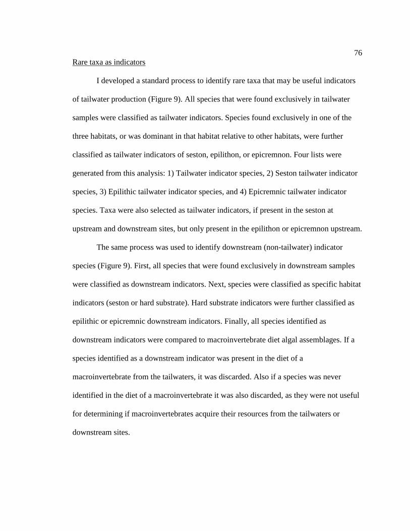
76
Rare taxa as indicators
I developed a standard process to identify rare taxa that may be useful indicators
of tailwater production (Figure 9). All species that were found exclusively in tailwater
samples were classified as tailwater indicators. Species found exclusively in one of the
three habitats, or was dominant in that habitat relative to other habitats, were further
classified as tailwater indicators of seston, epilithon, or epicremnon. Four lists were
generated from this analysis: 1) Tailwater indicator species, 2) Seston tailwater indicator
species, 3) Epilithic tailwater indicator species, and 4) Epicremnic tailwater indicator
species. Taxa were also selected as tailwater indicators, if present in the seston at
upstream and downstream sites, but only present in the epilithon or epicremnon upstream.
The same process was used to identify downstream (non-tailwater) indicator
species (Figure 9). First, all species that were found exclusively in downstream samples
were classified as downstream indicators. Next, species were classified as specific habitat
indicators (seston or hard substrate). Hard substrate indicators were further classified as
epilithic or epicremnic downstream indicators. Finally, all species identified as
downstream indicators were compared to macroinvertebrate diet algal assemblages. If a
species identified as a downstream indicator was present in the diet of a
macroinvertebrate from the tailwaters, it was discarded. Also if a species was never
identified in the diet of a macroinvertebrate it was also discarded, as they were not useful
for determining if macroinvertebrates acquire their resources from the tailwaters or
downstream sites.
77
Tailwater
indicator
Tailwater
indicator
Seston
indicator
Epilithon
indicator
Epicremnon
indicator
List of seston
indicator species
List of epilithon
indicator species
List of epicremnon
indicator species
Downstream
indicator
Downstream
indicator
Seston
indicator
Hard substrates
indicator
Hard substrates
indicator
List of epilithon
indicator species
List of epicremnon
indicator species
List of seston
indicator species
Figure 9. Flow chart used to classify tailwater and downstream indicator species.
Relative contribution of tailwater indicator species to macroinvertebrate production
Surface areas for each algal species were estimated from length and width
measurements of greater than ten cells for common species and from one to five cells for
rare species (note: geometric formulae approximating cell shapes were only applied for
circular and elliptical shaped cells, all other cell surface areas were estimated as the
product of the length and width). The relative surface area of each algal species was
calculated for each macroinvertebrate diet.
78
The proportion each tailwater indicator species comprised of the total surface area
in each macroinvertebrate’s diet algal assemblage was used to calculate the percent area
each tailwater indicator species comprised relative to the area of other particle types (ie
amorphous detritus, leaf material, other diatoms) consumed by each taxa (see Chapter 1).
Food-specific assimilation efficiencies (percentage of a food type that a
macroinvertebrate is able to assimilate) and net production efficiencies (an estimate of the
ratio of tissue production to energy assimilation) were used to estimate the relative
contribution of food types and tailwater indicator diatoms to production (see Chapter 1).
The relative contribution of each tailwater indicator diatom to macroinvertebrate
production was calculated for both the tailwaters and downstream sites, to estimate the
amount that tailwater diatoms may subsidize downstream macroinvertebrates.
Results
In this study, 159 algal species were identified from the sestonic, epilithic, and
epicremnic algal assemblages, and in the diets of S. arcticum and G. lacustris. Of these,
155 species were diatoms and four species were filamentous green algae. Despite the
relatively high species richness, fewer than 26 species comprised over 70 percent of most
communities (Figures 10, 11, and 12). Ultimately, five taxa were identified as tailwater
indicators and of these five, only two were present solely in the tailwaters. One seston
tailwater indicator, F. crotonensis, was chosen to assess the transport and survival of
algae downstream, because of its planktonic nature and dominance in the tailwater seston
community. Nine taxa were identified as downstream indicators, seven of which were
identified to species level.
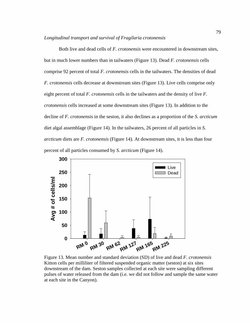
79
RM 0RM 30
RM 62RM 127
RM 165RM 225
Avg
# o
f ce
lls/m
l
0
50
100
150
200
250
300
Live Dead
Longitudinal transport and survival of Fragilaria crotonensis
Both live and dead cells of F. crotonensis were encountered in downstream sites,
but in much lower numbers than in tailwaters (Figure 13). Dead F. crotonensis cells
comprise 92 percent of total F. crotonensis cells in the tailwaters. The densities of dead
F. crotonensis cells decrease at downstream sites (Figure 13). Live cells comprise only
eight percent of total F. crotonensis cells in the tailwaters and the density of live F.
crotonensis cells increased at some downstream sites (Figure 13). In addition to the
decline of F. crotonensis in the seston, it also declines as a proportion of the S. arcticum
diet algal assemblage (Figure 14). In the tailwaters, 26 percent of all particles in S.
arcticum diets are F. crotonensis (Figure 14). At downstream sites, it is less than four
percent of all particles consumed by S. arcticum (Figure 14).
Figure 13. Mean number and standard deviation (SD) of live and dead F. crotonensis Kitton cells per milliliter of filtered suspended organic matter (seston) at six sites downstream of the dam. Seston samples collected at each site were sampling different pulses of water released from the dam (i.e. we did not follow and sample the same water at each site in the Canyon).
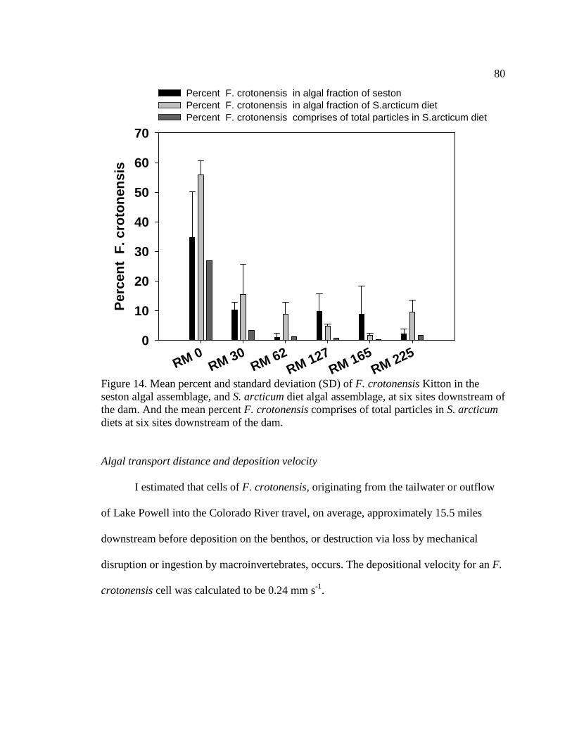
80
RM 0RM 30
RM 62RM 127
RM 165RM 225
Per
cen
t F
. cro
ton
ensi
s
0
10
20
30
40
50
60
70
Percent F. crotonensis in algal fraction of seston Percent F. crotonensis in algal fraction of S.arcticum diet Percent F. crotonensis comprises of total particles in S.arcticum diet
Figure 14. Mean percent and standard deviation (SD) of F. crotonensis Kitton in the seston algal assemblage, and S. arcticum diet algal assemblage, at six sites downstream of the dam. And the mean percent F. crotonensis comprises of total particles in S. arcticum diets at six sites downstream of the dam.
Algal transport distance and deposition velocity
I estimated that cells of F. crotonensis, originating from the tailwater or outflow
of Lake Powell into the Colorado River travel, on average, approximately 15.5 miles
downstream before deposition on the benthos, or destruction via loss by mechanical
disruption or ingestion by macroinvertebrates, occurs. The depositional velocity for an F.
crotonensis cell was calculated to be 0.24 mm s-1.
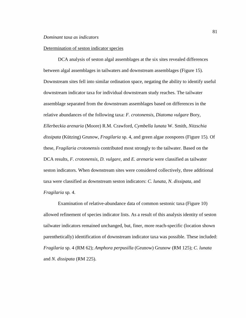
81
Dominant taxa as indicators
Determination of seston indicator species
DCA analysis of seston algal assemblages at the six sites revealed differences
between algal assemblages in tailwaters and downstream assemblages (Figure 15).
Downstream sites fell into similar ordination space, negating the ability to identify useful
downstream indicator taxa for individual downstream study reaches. The tailwater
assemblage separated from the downstream assemblages based on differences in the
relative abundances of the following taxa: F. crotonensis, Diatoma vulgare Bory,
Ellerbeckia arenaria (Moore) R.M. Crawford, Cymbella lunata W. Smith, Nitzschia
dissipata (Kützing) Grunow, Fragilaria sp. 4, and green algae zoospores (Figure 15). Of
these, Fragilaria crotonensis contributed most strongly to the tailwater. Based on the
DCA results, F. crotonensis, D. vulgare, and E. arenaria were classified as tailwater
seston indicators. When downstream sites were considered collectively, three additional
taxa were classified as downstream seston indicators: C. lunata, N. dissipata, and
Fragilaria sp. 4.
Examination of relative-abundance data of common sestonic taxa (Figure 10)
allowed refinement of species indicator lists. As a result of this analysis identity of seston
tailwater indicators remained unchanged, but, finer, more reach-specific (location shown
parenthetically) identification of downstream indicator taxa was possible. These included:
Fragilaria sp. 4 (RM 62); Amphora perpusilla (Grunow) Grunow (RM 125); C. lunata
and N. dissipata (RM 225).
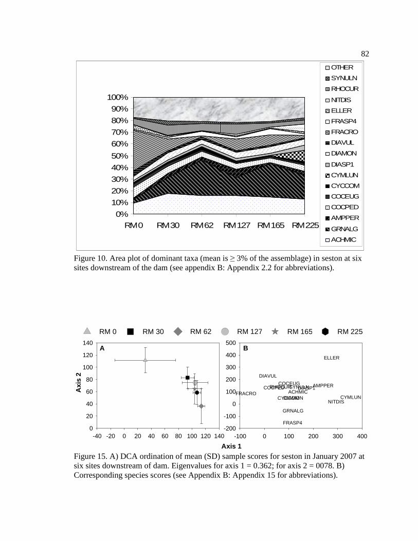
82
-40 -20 0 20 40 60 80 100 120 1400
20
40
60
80
100
120
140
-100 0 100 200 300 400-200
-100
0
100
200
300
400
500
ACHMIC
GRNALG
AMPPERCOCPEDCOCEUG
CYCCOM CYMLUN
DIASP1
DIAMON
DIAVUL
FRACRO
FRASP4
ELLER
NITDIS
RHOCURSYNULNAxi
s 2
Axis 1
A B
RM 0 RM 30 RM 62 RM 127 RM 165 RM 225RM 0 RM 30 RM 62 RM 127 RM 165 RM 225
0%
10%
20%
30%
40%
50%
60%
70%
80%
90%
100%
RM 0 RM 30 RM 62 RM 127 RM 165 RM 225
OTHER
SYNULN
RHOCUR
NITDIS
ELLER
FRASP4
FRACRO
DIAVUL
DIAMON
DIASP1
CYMLUN
CYCCOM
COCEUG
COCPED
AMPPER
GRNALG
ACHMIC
Figure 10. Area plot of dominant taxa (mean is ≥ 3% of the assemblage) in seston at six sites downstream of the dam (see appendix B: Appendix 2.2 for abbreviations). Figure 15. A) DCA ordination of mean (SD) sample scores for seston in January 2007 at six sites downstream of dam. Eigenvalues for axis 1 = 0.362; for axis 2 = 0078. B) Corresponding species scores (see Appendix B: Appendix 15 for abbreviations).
83
Determination of epilithon indicators
DCA analysis of epilithic algal assemblages at the six sites clearly separated algal
assemblages in the tailwaters from those downstream, with the greatest separations
between the tailwaters and RM 30 and 62 (the sites below the two largest tributaries)
(Figure 16). Differences were driven by the following taxa: Fragilaria sp. 4, Nitzschia
denticula Grunow/Denticula elegans Kützing, Synedra ulna (Nitzsch) Ehrenberg, D.
vulgare, A. perpusilla, Reimeria sinuata (Gregory) Kociolek & Stoermer, Encyonema
prostratrum (Berkeley) Kützing, E. arenaria, Nitzschia fonticola (Grunow) Grunow, and
Gyrosigma spencerii et varieties. Fragilaria sp. 4, N. denticula/D. elegans Kützing, S.
ulna, and D. vulgare were classified as tailwater indicators; and A. perpusilla, R. sinuata,
E. prostratrum, E. arenaria, N. fonticola, and G. spencerii et varieties, were classified as
downstream indicators.
Examination of relative-abundance data of common epilithic taxa (Figure 11)
allowed refinement of species indicator lists and more reach-specific (location shown
parenthetically) downstream indicator taxa were identified. Four additional downstream
indicator taxa were also identified. These included: A. perpusilla, E. prostratrum (RM 30
and 62); N. dissipata, N. fonticola, and G. spencerii et varieties (RM 127 and 165); R.
sinuata, Navicula cryptotenella Lange-Bertalot, Cymbella affinis Kützing, and Navicula
tripunctata (O.F. Müller) Bory (general downstream indicators).
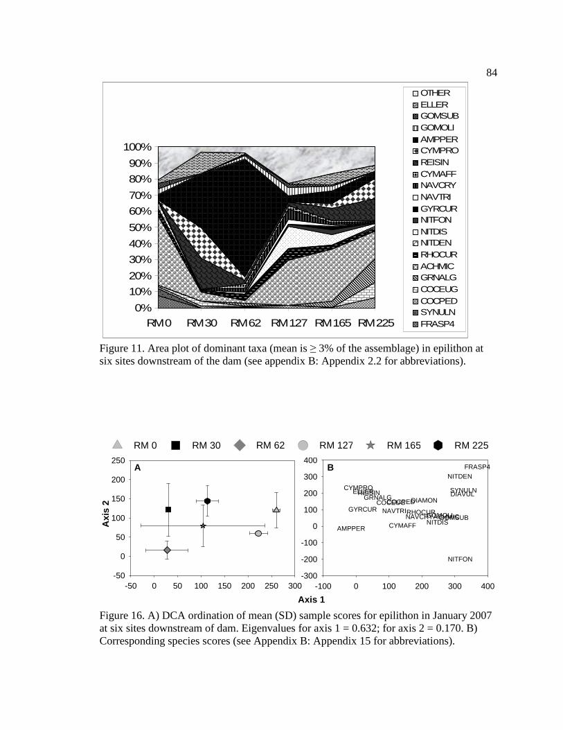
84
-50 0 50 100 150 200 250 300-50
0
50
100
150
200
250
-100 0 100 200 300 400-300
-200
-100
0
100
200
300
400
DIAVULDIAMON
FRASP4
SYNULN
COCPEDCOCEUGGRNALG
ACHMICRHOCUR
NITDEN
NITDIS
NITFON
GYRCUR NAVTRINAVCRY
CYMAFF
REISINCYMPRO
AMPPER
GOMOLIGOMSUB
ELLER
BA
Axis 1
Axi
s 2
RM 0 RM 30 RM 62 RM 127 RM 165 RM 225RM 0 RM 30 RM 62 RM 127 RM 165 RM 225
0%
10%
20%
30%
40%
50%
60%
70%
80%
90%
100%
RM 0 RM 30 RM 62 RM 127 RM 165 RM 225
OTHERELLERGOMSUBGOMOLIAMPPERCYMPROREISINCYMAFFNAVCRYNAVTRIGYRCURNITFONNITDISNITDENRHOCURACHMICGRNALGCOCEUGCOCPEDSYNULNFRASP4
Figure 11. Area plot of dominant taxa (mean is ≥ 3% of the assemblage) in epilithon at six sites downstream of the dam (see appendix B: Appendix 2.2 for abbreviations).
Figure 16. A) DCA ordination of mean (SD) sample scores for epilithon in January 2007 at six sites downstream of dam. Eigenvalues for axis 1 = 0.632; for axis 2 = 0.170. B) Corresponding species scores (see Appendix B: Appendix 15 for abbreviations).
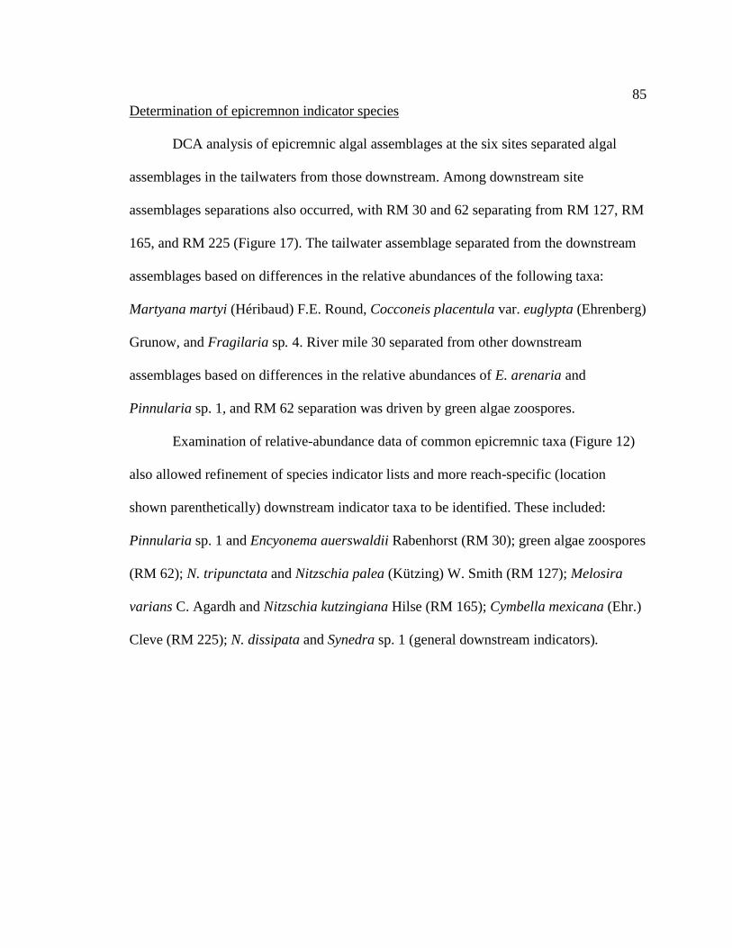
85
Determination of epicremnon indicator species
DCA analysis of epicremnic algal assemblages at the six sites separated algal
assemblages in the tailwaters from those downstream. Among downstream site
assemblages separations also occurred, with RM 30 and 62 separating from RM 127, RM
165, and RM 225 (Figure 17). The tailwater assemblage separated from the downstream
assemblages based on differences in the relative abundances of the following taxa:
Martyana martyi (Héribaud) F.E. Round, Cocconeis placentula var. euglypta (Ehrenberg)
Grunow, and Fragilaria sp. 4. River mile 30 separated from other downstream
assemblages based on differences in the relative abundances of E. arenaria and
Pinnularia sp. 1, and RM 62 separation was driven by green algae zoospores.
Examination of relative-abundance data of common epicremnic taxa (Figure 12)
also allowed refinement of species indicator lists and more reach-specific (location
shown parenthetically) downstream indicator taxa to be identified. These included:
Pinnularia sp. 1 and Encyonema auerswaldii Rabenhorst (RM 30); green algae zoospores
(RM 62); N. tripunctata and Nitzschia palea (Kützing) W. Smith (RM 127); Melosira
varians C. Agardh and Nitzschia kutzingiana Hilse (RM 165); Cymbella mexicana (Ehr.)
Cleve (RM 225); N. dissipata and Synedra sp. 1 (general downstream indicators).
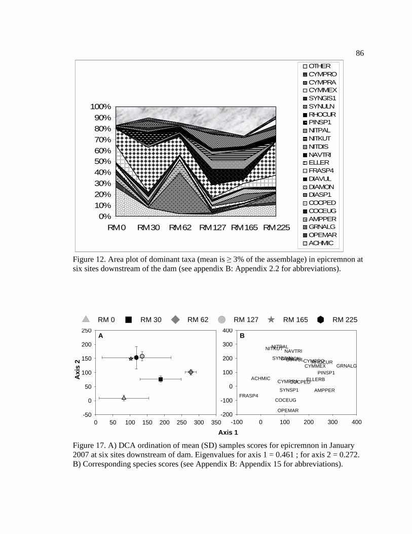
86
0%10%20%30%40%50%60%70%80%90%
100%
RM 0 RM 30 RM 62 RM 127 RM 165 RM 225
OTHERCYMPROCYMPRACYMMEXSYNGIS1SYNULNRHOCURPINSP1NITPALNITKUTNITDISNAVTRIELLERFRASP4DIAVULDIAMONDIASP1COCPEDCOCEUGAMPPERGRNALGOPEMARACHMIC
0 50 100 150 200 250 300 350-50
0
50
100
150
200
250
-100 0 100 200 300 400-200
-100
0
100
200
300
400
ACHMIC
AMPPER
COCEUG
COCPED
CYMMEX
CYMPRA
CYMPRODIAMONDIAVUL
ELLERB
FRASP4
GRNALG
NAVTRINITKUTNITPAL
OPEMAR
PINSP1
RHOCUR
SYNSP1
SYNULN
A B
Axi
s 2
Axis 1
RM 0 RM 30 RM 62 RM 127 RM 165 RM 225RM 0 RM 30 RM 62 RM 127 RM 165 RM 225
Figure 12. Area plot of dominant taxa (mean is ≥ 3% of the assemblage) in epicremnon at six sites downstream of the dam (see appendix B: Appendix 2.2 for abbreviations).
Figure 17. A) DCA ordination of mean (SD) samples scores for epicremnon in January 2007 at six sites downstream of dam. Eigenvalues for axis 1 = 0.461 ; for axis 2 = 0.272. B) Corresponding species scores (see Appendix B: Appendix 15 for abbreviations).
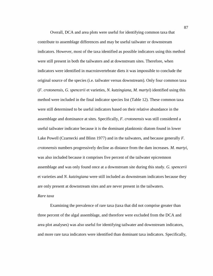
87
Overall, DCA and area plots were useful for identifying common taxa that
contribute to assemblage differences and may be useful tailwater or downstream
indicators. However, most of the taxa identified as possible indicators using this method
were still present in both the tailwaters and at downstream sites. Therefore, when
indicators were identified in macroinvertebrate diets it was impossible to conclude the
original source of the species (i.e. tailwater versus downstream). Only four common taxa
(F. crotonensis, G. spencerii et varieties, N. kutzingiana, M. martyi) identified using this
method were included in the final indicator species list (Table 12). These common taxa
were still determined to be useful indicators based on their relative abundance in the
assemblage and dominance at sites. Specifically, F. crotonensis was still considered a
useful tailwater indicator because it is the dominant planktonic diatom found in lower
Lake Powell (Czarnecki and Blinn 1977) and in the tailwaters, and because generally F.
crotonensis numbers progressively decline as distance from the dam increases. M. martyi,
was also included because it comprises five percent of the tailwater epicremnon
assemblage and was only found once at a downstream site during this study. G. spencerii
et varieties and N. kutzingiana were still included as downstream indicators because they
are only present at downstream sites and are never present in the tailwaters.
Rare taxa
Examining the prevalence of rare taxa (taxa that did not comprise greater than
three percent of the algal assemblage, and therefore were excluded from the DCA and
area plot analyses) was also useful for identifying tailwater and downstream indicators,
and more rare taxa indicators were identified than dominant taxa indicators. Specifically,
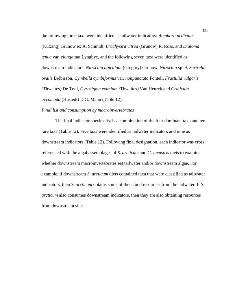
88
the following three taxa were identified as tailwater indicators: Amphora pediculus
(Kützing) Grunow ex A. Schmidt, Brachysira vitrea (Grunow) R. Ross, and Diatoma
tenue var. elongatum Lyngbye, and the following seven taxa were identified as
downstream indicators: Nitzschia apiculata (Gregory) Grunow, Nitzschia sp. 9, Surirella
ovalis Brébisson, Cymbella cymbiformis var. nonpunctata Fontell, Frustulia vulgaris
(Thwaites) De Toni, Gyrosigma eximium (Thwaites) Van Heurck,and Craticula
accomoda (Hustedt) D.G. Mann (Table 12).
Final list and consumption by macroinvertebrates
The final indicator species list is a combination of the four dominant taxa and ten
rare taxa (Table 12). Five taxa were identified as tailwater indicators and nine as
downstream indicators (Table 12). Following final designation, each indicator was cross
referenced with the algal assemblages of S. arcticum and G. lacustris diets to examine
whether downstream macroinvertebrates eat tailwater and/or downstream algae. For
example, if downstream S. arcticum diets contained taxa that were classified as tailwater
indicators, then S. arcticum obtains some of their food resources from the tailwater. If S.
arcticum also consumes downstream indicators, then they are also obtaining resources
from downstream sites.
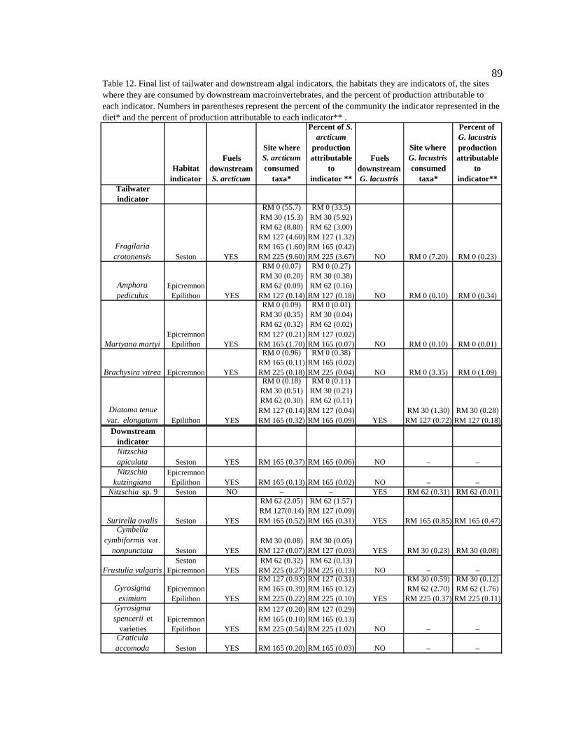
89
Habitat indicator
Fuels downstream S. arcticum
Site where S. arcticum consumed
taxa*
Percent of S. arcticum
production attributable
to indicator **
Fuels downstream G. lacustris
Site where G. lacustris consumed
taxa*
Percent of G. lacustris production attributable
to indicator**
Tailwater indicator
Fragilaria crotonensis Seston YES
RM 0 (55.7) RM 30 (15.3) RM 62 (8.80) RM 127 (4.60) RM 165 (1.60) RM 225 (9.60)
RM 0 (33.5) RM 30 (5.92) RM 62 (3.00) RM 127 (1.32) RM 165 (0.42) RM 225 (3.67) NO RM 0 (7.20) RM 0 (0.23)
Amphora pediculus
EpicremnonEpilithon YES
RM 0 (0.07) RM 30 (0.20) RM 62 (0.09) RM 127 (0.14)
RM 0 (0.27) RM 30 (0.38) RM 62 (0.16) RM 127 (0.18) NO RM 0 (0.10) RM 0 (0.34)
Martyana martyi Epicremnon
Epilithon YES
RM 0 (0.09) RM 30 (0.35) RM 62 (0.32) RM 127 (0.21) RM 165 (1.70)
RM 0 (0.01) RM 30 (0.04) RM 62 (0.02) RM 127 (0.02) RM 165 (0.07) NO RM 0 (0.10) RM 0 (0.01)
Brachysira vitrea Epicremnon YES
RM 0 (0.96) RM 165 (0.11) RM 225 (0.18)
RM 0 (0.38) RM 165 (0.02) RM 225 (0.04) NO RM 0 (3.35) RM 0 (1.09)
Diatoma tenue var. elongatum Epilithon YES
RM 0 (0.18) RM 30 (0.51) RM 62 (0.30) RM 127 (0.14) RM 165 (0.32)
RM 0 (0.11) RM 30 (0.21) RM 62 (0.11) RM 127 (0.04) RM 165 (0.09) YES
RM 30 (1.30) RM 127 (0.72)
RM 30 (0.28) RM 127 (0.18)
Downstream indicatorNitzschia apiculata Seston YES RM 165 (0.37) RM 165 (0.06) NO – –Nitzschia
kutzingiana Epicremnon
Epilithon YES RM 165 (0.13) RM 165 (0.02) NO – –Nitzschia sp. 9 Seston NO – – YES RM 62 (0.31) RM 62 (0.01)
Surirella ovalis Seston YES
RM 62 (2.05) RM 127(0.14) RM 165 (0.52)
RM 62 (1.57) RM 127 (0.09) RM 165 (0.31) YES RM 165 (0.85) RM 165 (0.47)
Cymbella cymbiformis var.
nonpunctata Seston YESRM 30 (0.08) RM 127 (0.07)
RM 30 (0.05) RM 127 (0.03) YES RM 30 (0.23) RM 30 (0.08)
Frustulia vulgaris Seston
Epicremnon YESRM 62 (0.32) RM 225 (0.27)
RM 62 (0.13) RM 225 (0.13) NO – –
Gyrosigma eximium
EpicremnonEpilithon YES
RM 127 (0.93) RM 165 (0.39) RM 225 (0.22)
RM 127 (0.31) RM 165 (0.12) RM 225 (0.10) YES
RM 30 (0.59) RM 62 (2.70) RM 225 (0.37)
RM 30 (0.12) RM 62 (1.76) RM 225 (0.11)
Gyrosigma spencerii et
varietiesEpicremnon
Epilithon YES
RM 127 (0.20) RM 165 (0.10) RM 225 (0.54)
RM 127 (0.29) RM 165 (0.13) RM 225 (1.02) NO – –
Craticula accomoda Seston YES RM 165 (0.20) RM 165 (0.03) NO – –
Table 12. Final list of tailwater and downstream algal indicators, the habitats they are indicators of, the sites where they are consumed by downstream macroinvertebrates, and the percent of production attributable to each indicator. Numbers in parentheses represent the percent of the community the indicator represented in the diet* and the percent of production attributable to each indicator** .
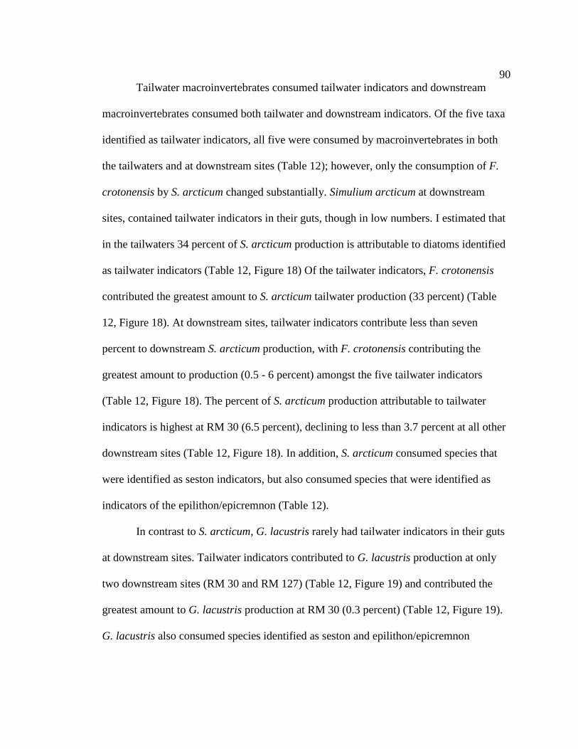
90
Tailwater macroinvertebrates consumed tailwater indicators and downstream
macroinvertebrates consumed both tailwater and downstream indicators. Of the five taxa
identified as tailwater indicators, all five were consumed by macroinvertebrates in both
the tailwaters and at downstream sites (Table 12); however, only the consumption of F.
crotonensis by S. arcticum changed substantially. Simulium arcticum at downstream
sites, contained tailwater indicators in their guts, though in low numbers. I estimated that
in the tailwaters 34 percent of S. arcticum production is attributable to diatoms identified
as tailwater indicators (Table 12, Figure 18) Of the tailwater indicators, F. crotonensis
contributed the greatest amount to S. arcticum tailwater production (33 percent) (Table
12, Figure 18). At downstream sites, tailwater indicators contribute less than seven
percent to downstream S. arcticum production, with F. crotonensis contributing the
greatest amount to production (0.5 - 6 percent) amongst the five tailwater indicators
(Table 12, Figure 18). The percent of S. arcticum production attributable to tailwater
indicators is highest at RM 30 (6.5 percent), declining to less than 3.7 percent at all other
downstream sites (Table 12, Figure 18). In addition, S. arcticum consumed species that
were identified as seston indicators, but also consumed species that were identified as
indicators of the epilithon/epicremnon (Table 12).
In contrast to S. arcticum, G. lacustris rarely had tailwater indicators in their guts
at downstream sites. Tailwater indicators contributed to G. lacustris production at only
two downstream sites (RM 30 and RM 127) (Table 12, Figure 19) and contributed the
greatest amount to G. lacustris production at RM 30 (0.3 percent) (Table 12, Figure 19).
G. lacustris also consumed species identified as seston and epilithon/epicremnon
91
RM 0RM 30
RM 62
RM 127
RM 165
RM 225
Per
cen
t
0
10
20
30
40
50
60
70
80
90
indicators, and in general consumed more epilithic/epicremnic indicator species than
seston indicator species.
Figure 18. Percent of S. arcticum production attributable to tailwater indicator diatoms, and all other non-indicator diatoms, at six sites downstream of the dam.
S. arcticum consumed all five tailwater indicators at downstream sites; however,
G. lacustris only consumed one tailwater indicator at a downstream site, D. tenue var.
elongatum. S. arcticum consumed more of the downstream indicators at more sites than
G. lacustris. S. arcticum consumed eight of the nine downstream indicators at
downstream sites and G. lacustris consumed four.
D. tenue var. elongatum F. crotonensis
Other Diatoms
M. martyi
B. vitrea A. pediculus
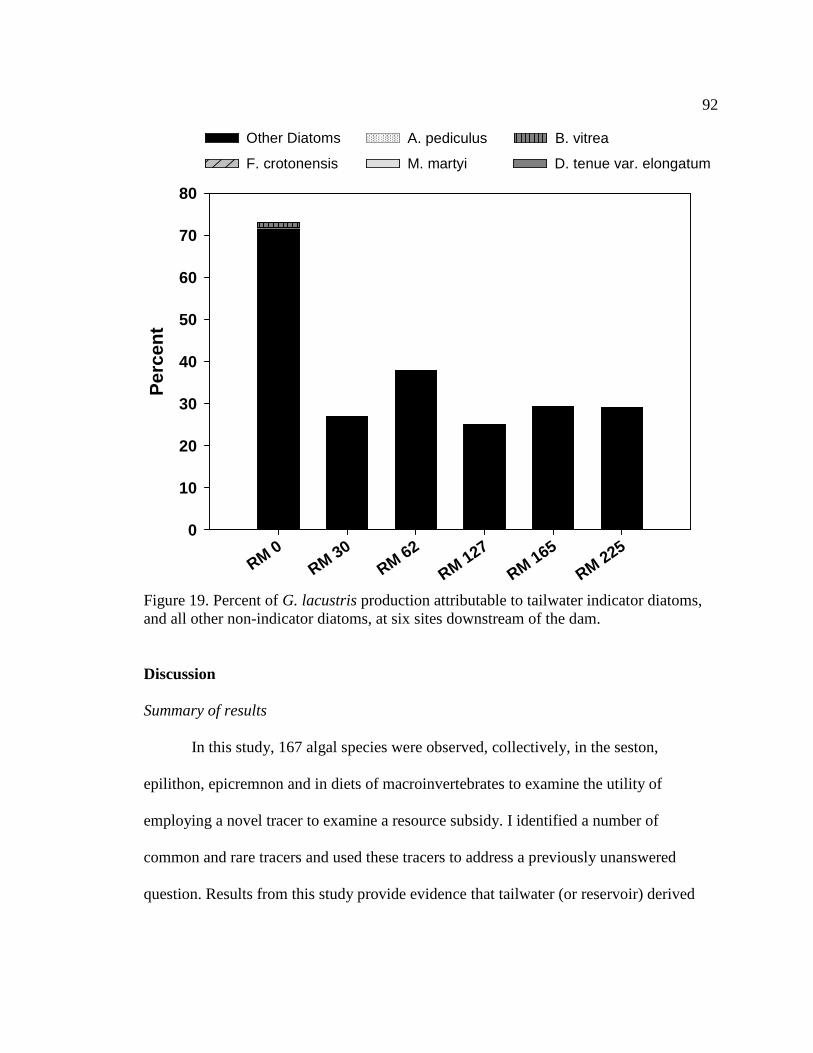
92
RM 0RM 30
RM 62
RM 127
RM 165
RM 225
Per
cen
t
0
10
20
30
40
50
60
70
80
Figure 19. Percent of G. lacustris production attributable to tailwater indicator diatoms, and all other non-indicator diatoms, at six sites downstream of the dam.
Discussion
Summary of results
In this study, 167 algal species were observed, collectively, in the seston,
epilithon, epicremnon and in diets of macroinvertebrates to examine the utility of
employing a novel tracer to examine a resource subsidy. I identified a number of
common and rare tracers and used these tracers to address a previously unanswered
question. Results from this study provide evidence that tailwater (or reservoir) derived
D. tenue var. elongatum F. crotonensis
Other Diatoms
M. martyi
B. vitrea A. pediculus
93
algae are consumed by downstream macroinvertebrates, although tailwater indicators
comprised less than 16 percent of diets and contributed less than 7 percent to
macroinvertebrate production at downstream sites. Filter-feeding macroinvertebrates like
S. arcticum are better suited to utilize upstream tailwater resources than scrapers such as
G. lacustris, which feed more locally. This technique may have general applicability to
other systems as well.
Algal downstream transport and survival
A euplanktonic species, F. crotonensis, was a useful indicator for this calculation,
because the source is most likely from Lake Powell inputs, it is most common in the
upper reaches, and its population is low throughout the canyon (Crayton and Sommerfeld
1979, Czarnecki and Blinn 1978). During downstream transport, mechanical destruction
of plankton in the water column can occur via the grinding action of riffles and rapids
laden with silt (Chandler 1937, Hartman and Himes 1961, Cushing 1964) and the decline
in the average number of F. crotonensis dead cells may be due to degradation and
destruction by rapids. In addition, because plankton can adhere to leaves and other
suspended particles and debris; inputs of organic matter from tributaries may accelerate
the settling and deposition of plankton onto the benthos (Chandler 1937). However, it is
unlikely that deposition is responsible for observed patterns of longitudinal decline of F.
crotonensis, as this taxon was rarely found in epilithic or epicremnic samples. In fact, the
average number of live cells of F. crotonensis increases at RM 127. Despite the increase
in live F. crotonensis cells at RM 127 and 165, this taxon comprised a small percentage
of both seston and S. arcticum diets at downstream sites. The decline in sestonic
94
representation may have been due to: 1) degradation or deposition of F. crotonensis or, 2)
dilution due to an increase in other diatoms from downstream sites or from epiphytes
detaching from drifting C. glomerata.
The increase in live cells at RM 127 and RM 165 may be due to a number of
factors: 1) there is a source population of F. crotonensis from a tributary above RM 127;
2) the live cells which survive through the rapids are reproducing downstream; 3)
because we are sampling different pulses of water at each site (i.e. we are not tracking the
same pulse of water) there may have been more live F. crotonensis cells transported from
the tailwaters in the pulse of water we sampled at those sites. In addition, because daily
discharge fluctuates in this system, increased discharge on some days may increase the
transport distance of plankton from lake outlets (Ward 1975, Armitage and Capper 1976,
Vadeboncoeur 1994). The increase in live cells suggests F. crotonensis is capable of
reproducing downstream or there are tributary source populations of F. crotonensis;
however, there is little evidence to support these hypotheses. F. crotonensis is a
euplanktonic diatom that is present in Lake Powell (Czarnecki and Blinn 1978) and
dominates the seston community in the tailwaters but not downstream. The
phytoplankton population in the river is dominated by tychoplankters (periphytic
organisms that become entrained in the water column due to turbulence, sloughing of the
filamentous algae to which they are attached, etc.) and few euplanktonic (organisms that
spend most or all of their lives as plankton) species, besides F. crotonensis, are present in
the river (Crayton and Sommerfeld 1979). Therefore, the likelihood of a source
population from one of the low discharge tributaries seems low especially because F.
95
crotonensis is typically planktonic, and there are not significant lakes and dams in
tributaries. The lakes and dams that are in tributaries are high in the watershed and are
connected to the mainstem only during times of extreme flooding. Furthermore, no
source population from tributaries has been reported. Extensive sampling of tributary
seston algal assemblages would help to clarify the source of live cells at downstream
sites. Turbidity, low water temperatures, high current velocity, and high variability in
water levels may also inhibit the production of euplanktonic diatoms at downstream sites
(Crayton and Sommerfeld 1979). Crayton and Sommerfield (1979) concluded there is
insufficient time for reproduction of plankton in the Colorado River due to the high flow
and short travel time of water through the canyon (ca. 3-4 days from Lake Powell to Lake
Mead); therefore, reproduction of F. crotonensis downstream seems unlikely. The
sampling of different pulses of water, with potentially different starting concentrations of
live F. crotonensis cells, at each site, may be the most plausible explanation for the
increase.
The decline in F. crotonensis provides evidence that the transport of
phytoplankton progressively declines as distance downstream increases, and
tailwater/lake resource use by macroinvertebrates also declines (Figure 6). A number of
studies document the decline of zooplankton (Ward 1975, Armitage and Capper 1976,
Sandlund 1982, Palmer and O’Keeffe 1990, Walks and Cyr 2004) and phytoplankton
(Maciolek and Tunzi 1968, Walks and Cyr 2004, Sabater et al. 2008) as distance
downstream from lakes or reservoirs increases. Likewise, recent food web studies using
stable isotopes, document that the importance of reservoir plankton subsidies to
96
downstream food webs declines with downstream distance from reservoirs (Doi et al.
2008, Mercado-Silva et al. 2008). Doi et al. 2008, estimated that zooplankton released
from Kanogawa Dam contributed significantly (from 20 -100 percent) to the diets of
collector-filterer macroinvertebrate diets 0.2 km below the dam, but within 10 km
contribution to macroinvertebrate diets decreased substantially (from 0 - 40 percent).
A number of factors can influence the downstream transport of particles and
plankton including mechanical degradation, destruction and sedimentation (Chandler
1937, Hartman and Himes 1961, Cushing 1964, Ward 1975), and removal by filter-
feeding organisms (Richardson and Mackay 1991, Monaghan et al. 2001) and aquatic
plants such as macrophytes (Chandler 1937, Horvath 2004). Hydrologic variables such as
discharge, turbulence, water depth and velocity (Wollheim et al. 2001, Hall et al. 1996,
Thomas et al. 2001) can also influence seston particle transport and deposition and lake-
outlet studies document that reservoir plankton are transported and persist further
downstream as discharge increases (Ward 1975, Armitage and Capper 1976,
Vadeboncoeur 1994).
In this study I estimated the expected transport distance before deposition (Sp) of
a tailwater diatom in the Colorado River to be 15.5 miles. Deposition velocity (Vdep) was
also calculated because it eliminates the scaling effect of depth and velocity on transport
distance (Thomas et al. 2001) and allows for comparison among streams with varying
water depths and velocities (i.e. discharge). F. crotonensis ranges in size from 40-170
µm. In comparison to studies with similar particle size ranges (15-1000 µm) the Vdep
(0.24 mm s-1) of F. crotonensis was similar to those reported elsewhere. Specifically, in a
97
first-order Idaho creek the diatom Asterionella (>52 µm) had a Vdep of 0.99 mm s-
1(Thomas et al. 2001), fine particulate organic matter (<1 mm) Vdep was 0.07-0.16 mm s-1
in second and third-order Idaho streams (Cushing et al. 1993), and settling velocity
(comparable to Vdep) of corn pollen (43-105 µm) was 0.263-0.311 16 mm s-1 in a
second-order stream in New York (Miller and Georgian 1992). Because the Vdep of F.
crotonensis is similar to the measured depositional velocities of other similar sized
particles, the estimated transport distance (Sp) of 15.5 miles seems accurate for this
system. Furthermore the Vdep estimate corresponds with the trends displayed in Figures 5
and 6, showing the greatest decline in F. crotonensis occurring in the first 30 miles, in
both the seston and S. arcticum diets.
The short transport distance of F. crotonensis, also provides evidence that
tailwater primary production may not effectively fuel the downstream food web. The
decline in F. crotonensis may be indicative of the declines that may be expected for other
tailwater diatoms. The low proportion of F. crotonensis in S. arcticum diets, demonstrates
the importance of diatoms produced at downstream sites, rather than those transported
from upstream, as a resource for filter-feeders. In addition, G. lacustris consumed species
identified as seston and epilithon/epicremnon indicators, demonstrating that diatoms in
the seston can be deposited on the benthos and consumed by macroinvertebrates.
However, F. crotonensis was only consumed by G. lacustris in the tailwaters; therefore,
the potential for other tailwater diatoms to be transported downstream, deposited, and
frequently consumed by macroinvertebrates seems unlikely.
98
Macroinvertebrate consumption of indicators
Tailwaters as a subsidy
Addressing the extent that tailwater primary production supports downstream
macroinvertebrate production requires the use of a tracer. Using tailwater and
downstream indicator species and measuring the extent to which macroinvertebrates
consume these species, I conclude that downstream macroinvertebrates rely on a
combination of tailwater and downstream food resources, including diatoms produced
within tributaries. Seston from reservoirs can be an important food resource for
consumers, particularly for collector-filterers, downstream of dams (Elliott and Corlett
1972, Petts 1984, Richardson 1984, Richardson and Mackay 1991, Voelz and Ward
1996, Doi et al. 2008). Of note, I found that S. arcticum consumed more tailwater
indicators at downstream sites than G. lacustris, suggesting that the extent that tailwater
resources can subsidize downstream macroinvertebrates depends on the functional
feeding groups present in the system (Doi et al 2008). S. arcticum is a collector-filterer
and can trap very small particles (Wotton 1976, Wotton 1977, Wallace and Merritt 1980),
planktonic species and tychoplankters that are sloughed from the epilithon or epicremnon
are accessible to these macroinvertebrates. In contrast, G. lacustris, a shredder, can only
consume species that are deposited on the benthos, and planktonic and tailwater algae
sloughed from the benthos and transported downstream may not be accessible. S.
arcticum consumed eight of the nine downstream indicators at downstream sites and G.
lacustris consumed four. Six of the downstream indicators were identified as seston
indicators and five were identified as epilithic/epicremnic indicators (Table 12) (note
99
total number of downstream habitat indicators does not equal nine because some species
were identified as indicators of both the seston and epilithon/epicremnon), again
indicating that tailwater and tributary resources may be a more important subsidy for
filter-feeding macroinvertebrates than shredders.
Consumption of downstream indicator taxa confirms the importance of
downstream resources in the diets of macroinvertebrates. It seems unlikely that
downstream macroinvertebrates are obtaining most of their resources from tailwater
primary production because tailwater indicator species are rarely consumed or are
consumed in extremely low proportions, and rare taxa that only grow downstream are
also consumed, even though they are not the dominant taxa present downstream. I
estimated that less than seven and 0.3 percent of S. arcticum and G. lacustris production,
respectively, may be attributable to tailwater indicators at downstream sites. This
estimate suggests that the tailwaters may not provide a significant resource subsidy to
downstream macroinvertebrate communities. Some macroinvertebrate production may be
derived from algal exudates or amorphous detritus derived from algae (Hart and Lovvorn
2003), but I estimated that autochthonously derived amorphous detritus contributed less
than eleven percent to macroinvertebrate production at downstream sites (Chapter 1).
DCA, area plots and rare taxa analysis for indicator identification
DCA, area plots, and analysis of the occurrence of rare taxa were useful for
identifying species that could be used as tailwater and downstream indicators. More rare
taxa were ultimately identified as indicators than dominant taxa, because dominant taxa
were often prevalent in both the tailwaters and downstream sites. In addition, more rare
100
taxa indicators were initially identified, but were ultimately discarded because their
presence was so infrequent or low that they were never consumed by macroinvertebrates.
Additional analyses of macroinvertebrate and habitat samples may allow for more rare
taxa to be utilized as indicators in the future.
Indicator presence and preferences
Five species were identified as tailwater indicators and, of these five, only two, B.
vitrea and D. tenue var. elongatum, were found solely in the tailwaters. The other three
taxa, F. crotonensis, A. pediculus, and M. martyi were also present at downstream sites;
however, A. pediculus and M. martyi were only present at one site in extremely low
proportions, and therefore were still considered tailwater indicators. B. vitrea and A.
pediculus have also previously been reported at downstream sites (Czarnecki and Blinn
1978). B. vitrea has been reported in Clear and Diamond Creeks, but is also found in
lower Lake Powell. A. pediculus has been reported in epiphytic collections throughout the
canyon (in low numbers), but is known to prefer filamentous algae or large diatoms as a
substrate, which may explain their preference for the tailwaters in these samples (Patrick
and Reimer 1966, Czarnecki and Blinn 1978). F. crotonensis and D. tenue var. elongatum
appear to be the best tailwater indicators; however, analyzing more samples from other
seasons may help to identify additional tailwater indicators.
Nine taxa were identified as downstream indicators. Eight of these nine were
identified to species level and their ecological preferences reflected the change from clear
(tailwaters) to turbid (downstream) water conditions. C. accomoda thrives in the presence
of high organics (Patrick and Reimer 1966) and has been previously collected from
101
epipelic and psammon collections (which tend to be higher in organics than the epilithon)
in Kanab and Bright Angel Creek (Czarnecki and Blinn 1978). C. cymbiformis var.
nonpunctata has only been previously collected in epilithic samples (these collections
were associated with fine particulate material) of Elves Chasm (RM 116.5) (Czarnecki
and Blinn 1978). S. ovalis is an epipelic species found in the Little Colorado River
(although it also has been reported from the Lake Powell area) (Czarnecki and Blinn
1978, Kelly et al. 2005). In my samples, S. ovalis was not collected until downstream of
the confluence with the Little Colorado River. Because this taxon is consumed by
macroinvertebrates in the mainstem, it confirms that tributary resources are used by
downstream macroinvertebrates; however, this taxon contributes less than two percent to
macroinvertebrate production at downstream sites (Table 12). Gyrosigma spp. are also
typically epipelic (Kelly et al 2005) and therefore do well at downstream sites. N.
kutzingiana and N. apiculata have been reported to be common in lower Lake Powell and
throughout the Colorado River system of the Grand Canyon and may not be appropriate
to use as downstream indicators (Czarnecki and Blinn 1978). F. vulgaris is also reported
to be common throughout the system (Czarnecki and Blinn 1978), but it has never been
observed in Lake Powell and has only been collected downstream in our samples. In
conclusion, C. accomoda, C. cymbiformis var. nonpunctata, S. ovalis, F. vulgaris and
Gyrosigma spp. may serve as the best downstream indicators in this system.
Utility of the method/usefulness of algae as indicators/tracers
This method was useful for examining the consumption of tailwater algal taxa by
downstream macroinvertebrates and helped to address whether downstream food webs
102
are fueled by autochthonous resources produced in the tailwaters (Carothers and Brown
1991). Assessing differences using the dominant taxa in the system established that algal
assemblages at each site were not sufficiently different to distinguish among the
downstream sites, but were useful for distinguishing between the tailwaters and
downstream. Downstream assemblages did differ from the tailwater assemblages;
however, because the taxa that drove the differences were common throughout the
system, few were determined to be useful indicators (tracers). Rare taxa were better
indicators because of their ecological preferences and specificity to tailwater or
downstream sites.
Although this method helped to address an important question relating to an
ecological subsidy, the required algal community analyses to the species level in a system
with high algal species diversity, resulted in an extremely time-consuming process. In
addition, this method can only be used in systems where there are community differences
among sites and therefore species can be classified as site-specific indicators. The
physical and chemical conditions in the Colorado River differ among the tailwaters and
downstream sites and I was able to identify useful indicators. In more uniform systems, it
may be difficult to identify indicators; therefore, using algae as tracers may only be
useful in some systems. Other tracer techniques may be employed to further examine the
extent to which the tailwaters provide an ecological subsidy to downstream food webs.
For example, diatoms labeled with 14C sodium bicarbonate were used to examine seston
transport and deposition in Idaho streams (Thomas et al. 2001), and fluorescently labeled
bacteria (FLB) were used to examine bacterial transport and consumption by
103
macroinvertebrates in a second-order stream in North Carolina (Hall et al. 1996).
Although both of these methods were used in streams much smaller than the Colorado
River, exploring the potential use of labeled particles to address the importance of
tailwater and reservoir subsidies to downstream systems may be valuable.
Conclusion
In conclusion, primary production in tailwaters (or upstream reservoirs) of rivers
may subsidize downstream macroinvertebrates; however, the importance of the subsidy
may decline with distance downstream from the dam. The suggestion that the highly
productive tailwaters below Glen Canyon Dam serve as a resource subsidy to
downstream food webs is partially correct, because downstream macroinvertebrates
consume algae produced in the tailwaters. However, macroinvertebrates also consume
algae produced at downstream sites and tailwaters indicators were estimated to contribute
less than seven percent to downstream macroinvertebrate production. Furthermore, algae
produced in the tailwaters of the dam or lake are capable of being transported
downstream, but their numbers and dominance in the community decline as distance
from the tailwater increases.
I also estimated the transport distance of planktonic diatoms or diatoms sloughed
into the seston is 15.5 miles (25 km); therefore, most of the production exported from
tailwaters may not be transported far enough and in a form that can fuel
macroinvertebrate production throughout the 226 mile (363 km) stretch of river through
the Grand Canyon. Macroinvertebrates are an important food resource for fish (Childs et
al. 1998, Zahn et al. unpublished data), and an important goal of scientists and managers
104
in this system is to better manage dam operations to increase and support native fish
production, particularly the endangered humpback chub. The largest and only
successfully reproducing population of humpback chub in the Canyon is located near the
confluence of the Colorado and Little Colorado Rivers, 61 miles downstream from the
dam (Gloss and Coggins 2005). Because tailwater primary production may only serve as
an important subsidy up to 15.5 miles downstream of the dam, macroinvertebrates and
native fish at downstream sites may be supported by other food resources, and managing
the system to maximize access to these resources may be an important task.

105
APPENDIX A
ONE-WAY ANOVA TABLES
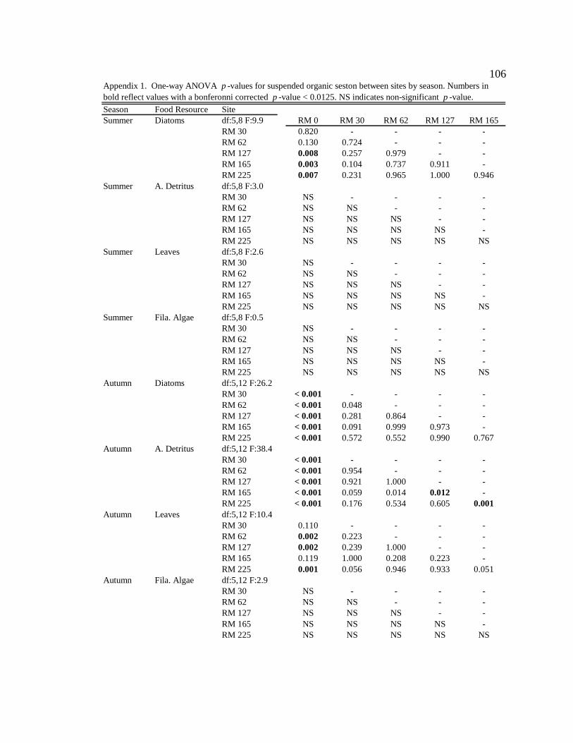
106
Season Food Resource SiteSummer Diatoms df:5,8 F:9.9 RM 0 RM 30 RM 62 RM 127 RM 165
RM 30 0.820 - - - -RM 62 0.130 0.724 - - -RM 127 0.008 0.257 0.979 - -RM 165 0.003 0.104 0.737 0.911 -RM 225 0.007 0.231 0.965 1.000 0.946
Summer A. Detritus df:5,8 F:3.0RM 30 NS - - - -RM 62 NS NS - - -RM 127 NS NS NS - -RM 165 NS NS NS NS -RM 225 NS NS NS NS NS
Summer Leaves df:5,8 F:2.6RM 30 NS - - - -RM 62 NS NS - - -RM 127 NS NS NS - -RM 165 NS NS NS NS -RM 225 NS NS NS NS NS
Summer Fila. Algae df:5,8 F:0.5RM 30 NS - - - -RM 62 NS NS - - -RM 127 NS NS NS - -RM 165 NS NS NS NS -RM 225 NS NS NS NS NS
Autumn Diatoms df:5,12 F:26.2RM 30 < 0.001 - - - -RM 62 < 0.001 0.048 - - -RM 127 < 0.001 0.281 0.864 - -RM 165 < 0.001 0.091 0.999 0.973 -RM 225 < 0.001 0.572 0.552 0.990 0.767
Autumn A. Detritus df:5,12 F:38.4RM 30 < 0.001 - - - -RM 62 < 0.001 0.954 - - -RM 127 < 0.001 0.921 1.000 - -RM 165 < 0.001 0.059 0.014 0.012 -RM 225 < 0.001 0.176 0.534 0.605 0.001
Autumn Leaves df:5,12 F:10.4RM 30 0.110 - - - -RM 62 0.002 0.223 - - -RM 127 0.002 0.239 1.000 - -RM 165 0.119 1.000 0.208 0.223 -RM 225 0.001 0.056 0.946 0.933 0.051
Autumn Fila. Algae df:5,12 F:2.9RM 30 NS - - - -RM 62 NS NS - - -RM 127 NS NS NS - -RM 165 NS NS NS NS -RM 225 NS NS NS NS NS
Appendix 1. One-way ANOVA p -values for suspended organic seston between sites by season. Numbers in bold reflect values with a bonferonni corrected p -value < 0.0125. NS indicates non-significant p -value.
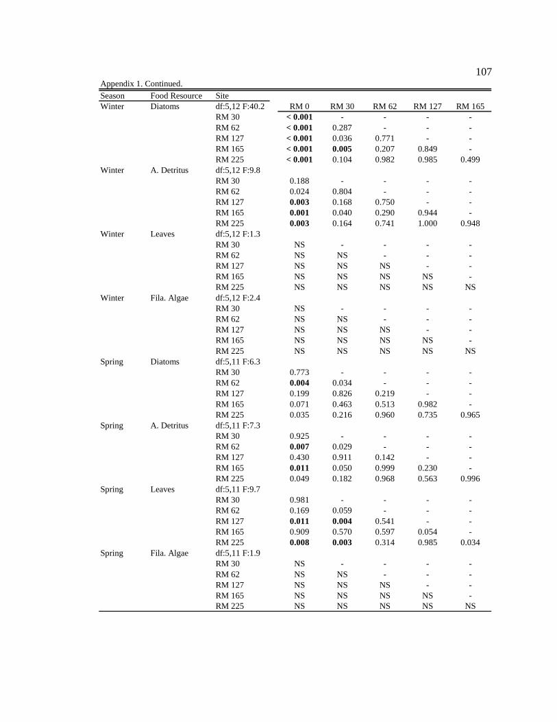
107
Appendix 1. Continued.
Season Food Resource SiteWinter Diatoms df:5,12 F:40.2 RM 0 RM 30 RM 62 RM 127 RM 165
RM 30 < 0.001 - - - -RM 62 < 0.001 0.287 - - -RM 127 < 0.001 0.036 0.771 - -RM 165 < 0.001 0.005 0.207 0.849 -RM 225 < 0.001 0.104 0.982 0.985 0.499
Winter A. Detritus df:5,12 F:9.8RM 30 0.188 - - - -RM 62 0.024 0.804 - - -RM 127 0.003 0.168 0.750 - -RM 165 0.001 0.040 0.290 0.944 -RM 225 0.003 0.164 0.741 1.000 0.948
Winter Leaves df:5,12 F:1.3RM 30 NS - - - -RM 62 NS NS - - -RM 127 NS NS NS - -RM 165 NS NS NS NS -RM 225 NS NS NS NS NS
Winter Fila. Algae df:5,12 F:2.4RM 30 NS - - - -RM 62 NS NS - - -RM 127 NS NS NS - -RM 165 NS NS NS NS -RM 225 NS NS NS NS NS
Spring Diatoms df:5,11 F:6.3RM 30 0.773 - - - -RM 62 0.004 0.034 - - -RM 127 0.199 0.826 0.219 - -RM 165 0.071 0.463 0.513 0.982 -RM 225 0.035 0.216 0.960 0.735 0.965
Spring A. Detritus df:5,11 F:7.3RM 30 0.925 - - - -RM 62 0.007 0.029 - - -RM 127 0.430 0.911 0.142 - -RM 165 0.011 0.050 0.999 0.230 -RM 225 0.049 0.182 0.968 0.563 0.996
Spring Leaves df:5,11 F:9.7RM 30 0.981 - - - -RM 62 0.169 0.059 - - -RM 127 0.011 0.004 0.541 - -RM 165 0.909 0.570 0.597 0.054 -RM 225 0.008 0.003 0.314 0.985 0.034
Spring Fila. Algae df:5,11 F:1.9RM 30 NS - - - -RM 62 NS NS - - -RM 127 NS NS NS - -RM 165 NS NS NS NS -RM 225 NS NS NS NS NS
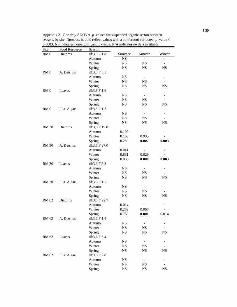
108
Site Food Resource SeasonRM 0 Diatoms df:3,8 F:1.8 Summer Autumn Winter
Autumn NS - -Winter NS NS -Spring NS NS NS
RM 0 A. Detritus df:3,8 F:6.5Autumn NS - -Winter NS NS -Spring NS NS NS
RM 0 Leaves df:3,8 F:1.6Autumn NS - -Winter NS NS -Spring NS NS NS
RM 0 Fila. Algae df:3,8 F:1.2Autumn NS - -Winter NS NS -Spring NS NS NS
RM 30 Diatoms df:3,6 F:19.8Autumn 0.100 - -Winter 0.165 0.935 -Spring 0.289 0.002 0.003
RM 30 A. Detritus df:3,6 F:37.0Autumn 0.041 - -Winter 0.831 0.029 -Spring 0.036 0.000 0.003
RM 30 Leaves df:3,6 F:3.3Autumn NS - -Winter NS NS -Spring NS NS NS
RM 30 Fila. Algae df:3,6 F:1.5Autumn NS - -Winter NS NS -Spring NS NS NS
RM 62 Diatoms df:3,6 F:22.7Autumn 0.014 - -Winter 0.202 0.060 -Spring 0.763 0.001 0.014
RM 62 A. Detritus df:3,6 F:1.4Autumn NS - -Winter NS NS -Spring NS NS NS
RM 62 Leaves df:3,6 F:3.4Autumn NS - -Winter NS NS -Spring NS NS NS
RM 62 Fila. Algae df:3,6 F:2.8Autumn NS - -Winter NS NS -Spring NS NS NS
Appendix 2. One-way ANOVA p-values for suspended organic seston between seasons by site. Numbers in bold reflect values with a bonferonni corrected p -value < 0.0083. NS indicates non-significant p -value. N/A indicates no data available.
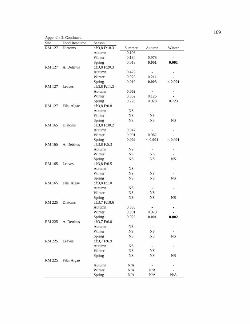
109
Appendix 2. Continued.
Site Food Resource SeasonRM 127 Diatoms df:3,8 F:18.3 Summer Autumn Winter
Autumn 0.106 - -Winter 0.184 0.978 -Spring 0.018 0.001 0.001
RM 127 A. Detritus df:3,8 F:20.3Autumn 0.476 - -Winter 0.026 0.211 -Spring 0.019 0.003 < 0.001
RM 127 Leaves df:3,8 F:11.3Autumn 0.002 - -Winter 0.052 0.125 -Spring 0.228 0.028 0.723
RM 127 Fila. Algae df:3,8 F:0.8Autumn NS - -Winter NS NS -Spring NS NS NS
RM 165 Diatoms df:3,8 F:30.2Autumn 0.047 - -Winter 0.091 0.962 -Spring 0.004 < 0.001 < 0.001
RM 165 A. Detritus df:3,8 F:5.3Autumn NS - -Winter NS NS -Spring NS NS NS
RM 165 Leaves df:3,8 F:0.5Autumn NS - -Winter NS NS -Spring NS NS NS
RM 165 Fila. Algae df:3,8 F:1.0Autumn NS - -Winter NS NS -Spring NS NS NS
RM 225 Diatoms df:3,7 F:18.6Autumn 0.055 - -Winter 0.091 0.979 -Spring 0.026 0.001 0.002
RM 225 A. Detritus df:3,7 F:6.0Autumn NS - -Winter NS NS -Spring NS NS NS
RM 225 Leaves df:3,7 F:6.9Autumn NS - -Winter NS NS -Spring NS NS NS
RM 225 Fila. AlgaeAutumn N/A - -Winter N/A N/A -Spring N/A N/A N/A

110
Season Food Resource SiteSummer Diatoms df:5,12 F:3.4 RM 0 RM 30 RM 62 RM 127 RM 165
RM 30 NS - - - -RM 62 NS NS - - -RM 127 NS NS NS - -RM 165 NS NS NS NS -RM 225 NS NS NS NS NS
Summer A. Detritus df:5,12 F:5.7RM 30 0.693 - - - -RM 62 0.089 0.594 - - -RM 127 0.081 0.668 1.000 - -RM 165 0.069 0.616 1.000 1.000 -RM 225 0.004 0.068 0.825 0.571 0.623
Summer Leaves df:5,12 F:4.5RM 30 0.155 - - - -RM 62 0.457 0.997 - - -RM 127 0.007 0.509 0.376 - -RM 165 0.080 0.999 0.964 0.728 -RM 225 0.133 1.000 0.994 0.561 1.000
Summer Fila. Algae df:5,12 F:16.5RM 30 < 0.001 - - - -RM 62 0.001 1.000 - - -RM 127 < 0.001 1.000 1.000 - -RM 165 < 0.001 1.000 1.000 1.000 -RM 225 < 0.001 1.000 1.000 1.000 1.000
Autumn Diatoms df:5,11 F:2.8RM 30 NS - - - -RM 62 NS NS - - -RM 127 NS NS NS - -RM 165 NS NS NS NS -RM 225 NS NS NS NS NS
Autumn A. Detritus df:5,11 F:6.7RM 30 0.011 - - - -RM 62 0.026 1.000 - - -RM 127 0.003 0.961 0.961 - -RM 165 0.040 0.959 0.985 0.604 -RM 225 0.214 0.452 0.609 0.152 0.879
Autumn Leaves df:5,11 F:1.1RM 30 NS - - - -RM 62 NS NS - - -RM 127 NS NS NS - -RM 165 NS NS NS NS -RM 225 NS NS NS NS NS
Autumn Fila. Algae df:5,11 F:1.4RM 30 NS - - - -RM 62 NS NS - - -RM 127 NS NS NS - -RM 165 NS NS NS NS -RM 225 NS NS NS NS NS
Appendix 3. One-way ANOVA p -values for epilithon between sites by season. Numbers in bold reflect values with a bonferonni corrected p-value < 0.0125. NS indicates non-significant p -value.
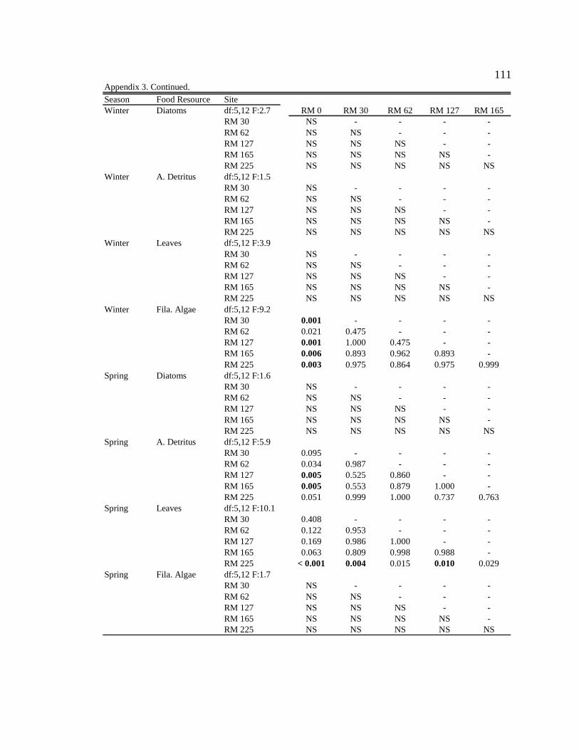
111
Appendix 3. Continued.
Season Food Resource SiteWinter Diatoms df:5,12 F:2.7 RM 0 RM 30 RM 62 RM 127 RM 165
RM 30 NS - - - -RM 62 NS NS - - -RM 127 NS NS NS - -RM 165 NS NS NS NS -RM 225 NS NS NS NS NS
Winter A. Detritus df:5,12 F:1.5RM 30 NS - - - -RM 62 NS NS - - -RM 127 NS NS NS - -RM 165 NS NS NS NS -RM 225 NS NS NS NS NS
Winter Leaves df:5,12 F:3.9RM 30 NS - - - -RM 62 NS NS - - -RM 127 NS NS NS - -RM 165 NS NS NS NS -RM 225 NS NS NS NS NS
Winter Fila. Algae df:5,12 F:9.2RM 30 0.001 - - - -RM 62 0.021 0.475 - - -RM 127 0.001 1.000 0.475 - -RM 165 0.006 0.893 0.962 0.893 -RM 225 0.003 0.975 0.864 0.975 0.999
Spring Diatoms df:5,12 F:1.6RM 30 NS - - - -RM 62 NS NS - - -RM 127 NS NS NS - -RM 165 NS NS NS NS -RM 225 NS NS NS NS NS
Spring A. Detritus df:5,12 F:5.9RM 30 0.095 - - - -RM 62 0.034 0.987 - - -RM 127 0.005 0.525 0.860 - -RM 165 0.005 0.553 0.879 1.000 -RM 225 0.051 0.999 1.000 0.737 0.763
Spring Leaves df:5,12 F:10.1RM 30 0.408 - - - -RM 62 0.122 0.953 - - -RM 127 0.169 0.986 1.000 - -RM 165 0.063 0.809 0.998 0.988 -RM 225 < 0.001 0.004 0.015 0.010 0.029
Spring Fila. Algae df:5,12 F:1.7RM 30 NS - - - -RM 62 NS NS - - -RM 127 NS NS NS - -RM 165 NS NS NS NS -RM 225 NS NS NS NS NS

112
Site Food Resource SeasonRM 0 Diatoms df:3,9 F:1.1 Summer Autumn Winter
Autumn NS - -Winter NS NS -Spring NS NS NS
RM 0 A. Detritus df:3,9 F:4.2Autumn NS - -Winter NS NS -Spring NS NS NS
RM 0 Leaves df:3,9 F:6.8Autumn NS - -Winter NS NS -Spring NS NS NS
RM 0 Fila. Algae df:3,9 F:1.3Autumn NS - -Winter NS NS -Spring NS NS NS
RM 30 Diatoms df:3,8 F:9.5Autumn 0.024 - -Winter 0.092 0.768 -Spring 0.833 0.008 0.028
RM 30 A. Detritus df:3,8 F:12.8Autumn 0.003 - -Winter 0.089 0.120 -Spring 0.998 0.004 0.114
RM 30 Leaves df:3,8 F:7.6Autumn NS - -Winter NS NS -Spring NS NS NS
RM 30 Fila. Algae df:3,8 F:1.0Autumn NS - -Winter NS NS -Spring NS NS NS
RM 62 Diatoms df:3,6 F:4.1Autumn NS - -Winter NS NS -Spring NS NS NS
RM 62 A. Detritus df:3,6 F:5.9Autumn NS - -Winter NS NS -Spring NS NS NS
RM 62 Leaves df:3,6 F:3.6Autumn NS - -Winter NS NS -Spring NS NS NS
RM 62 Fila. Algae df:3,6 F:1.5Autumn NS - -Winter NS NS -Spring NS NS NS
Appendix 4. One-way ANOVA p-values for epilithon between seasons by site. Numbers in bold reflect values with a bonferonni corrected p -value < 0.0083. NS indicates non-significant p -value. N/A indicates no data available.
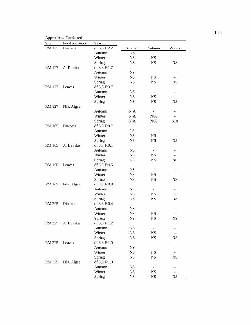
113
Appendix 4. Continued.
Site Food Resource SeasonRM 127 Diatoms df:3,8 F:2.2 Summer Autumn Winter
Autumn NS - -Winter NS NS -Spring NS NS NS
RM 127 A. Detritus df:3,8 F:1.7Autumn NS - -Winter NS NS -Spring NS NS NS
RM 127 Leaves df:3,8 F:3.7Autumn NS - -Winter NS NS -Spring NS NS NS
RM 127 Fila. AlgaeAutumn N/A - -Winter N/A N/A -Spring N/A N/A N/A
RM 165 Diatoms df:3,8 F:0.7Autumn NS - -Winter NS NS -Spring NS NS NS
RM 165 A. Detritus df:3,8 F:0.1Autumn NS - -Winter NS NS -Spring NS NS NS
RM 165 Leaves df:3,8 F:4.5Autumn NS - -Winter NS NS -Spring NS NS NS
RM 165 Fila. Algae df:3,8 F:0.8Autumn NS - -Winter NS NS -Spring NS NS NS
RM 225 Diatoms df:3,8 F:0.4Autumn NS - -Winter NS NS -Spring NS NS NS
RM 225 A. Detritus df:3,8 F:1.2Autumn NS - -Winter NS NS -Spring NS NS NS
RM 225 Leaves df:3,8 F:1.0Autumn NS - -Winter NS NS -Spring NS NS NS
RM 225 Fila. Algae df:3,8 F:1.0Autumn NS - -Winter NS NS -Spring NS NS NS
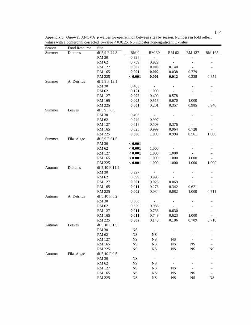
114
Season Food Resource SiteSummer Diatoms df:5,9 F:22.8 RM 0 RM 30 RM 62 RM 127 RM 165
RM 30 0.998 - - - -RM 62 0.759 0.922 - - -RM 127 0.002 0.008 0.140 - -RM 165 0.001 0.002 0.038 0.779 -RM 225 < 0.001 0.001 0.012 0.238 0.854
Summer A. Detritus df:5,9 F:13.1RM 30 0.463 - - - -RM 62 0.121 1.000 - - -RM 127 0.002 0.409 0.578 - -RM 165 0.005 0.515 0.670 1.000 -RM 225 0.001 0.201 0.357 0.985 0.946
Summer Leaves df:5,9 F:6.5RM 30 0.493 - - - -RM 62 0.749 0.997 - - -RM 127 0.018 0.509 0.376 - -RM 165 0.025 0.999 0.964 0.728 -RM 225 0.008 1.000 0.994 0.561 1.000
Summer Fila. Algae df:5,9 F:61.5RM 30 < 0.001 - - - -RM 62 < 0.001 1.000 - - -RM 127 < 0.001 1.000 1.000 - -RM 165 < 0.001 1.000 1.000 1.000 -RM 225 < 0.001 1.000 1.000 1.000 1.000
Autumn Diatoms df:5,10 F:11.4RM 30 0.327 - - - -RM 62 0.899 0.995 - - -RM 127 0.001 0.026 0.069 - -RM 165 0.011 0.276 0.342 0.621 -RM 225 0.002 0.034 0.082 1.000 0.711
Autumn A. Detritus df:5,10 F:8.2RM 30 0.086 - - - -RM 62 0.629 0.986 - - -RM 127 0.011 0.758 0.630 - -RM 165 0.011 0.749 0.623 1.000 -RM 225 0.002 0.143 0.186 0.709 0.718
Autumn Leaves df:5,10 F:1.5RM 30 NS - - - -RM 62 NS NS - - -RM 127 NS NS NS - -RM 165 NS NS NS NS -RM 225 NS NS NS NS NS
Autumn Fila. Algae df:5,10 F:0.5RM 30 NS - - - -RM 62 NS NS - - -RM 127 NS NS NS - -RM 165 NS NS NS NS -RM 225 NS NS NS NS NS
Appendix 5. One-way ANOVA p -values for epicremnon between sites by season. Numbers in bold reflect values with a bonferonni corrected p-value < 0.0125. NS indicates non-significant p-value.
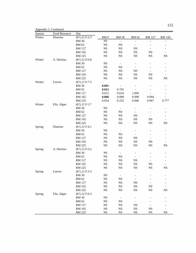
115
Appendix 5. Continued.
Season Food Resource SiteWinter Diatoms df:5,12 F:2.3 RM 0 RM 30 RM 62 RM 127 RM 165
RM 30 NS - - - -RM 62 NS NS - - -RM 127 NS NS NS - -RM 165 NS NS NS NS -RM 225 NS NS NS NS NS
Winter A. Detritus df:5,12 F:0.8RM 30 NS - - - -RM 62 NS NS - - -RM 127 NS NS NS - -RM 165 NS NS NS NS -RM 225 NS NS NS NS NS
Winter Leaves df:5,12 F:7.5RM 30 0.001 - - - -RM 62 0.012 0.705 - - -RM 127 0.015 0.634 1.000 - -RM 165 0.006 0.898 0.998 0.994 -RM 225 0.054 0.252 0.940 0.967 0.777
Winter Fila. Algae df:5,12 F:1.7RM 30 NS - - - -RM 62 NS NS - - -RM 127 NS NS NS - -RM 165 NS NS NS NS -RM 225 NS NS NS NS NS
Spring Diatoms df:5,12 F:4.1RM 30 NS - - - -RM 62 NS NS - - -RM 127 NS NS NS - -RM 165 NS NS NS NS -RM 225 NS NS NS NS NS
Spring A. Detritus df:5,12 F:3.2RM 30 NS - - - -RM 62 NS NS - - -RM 127 NS NS NS - -RM 165 NS NS NS NS -RM 225 NS NS NS NS NS
Spring Leaves df:5,12 F:3.3RM 30 NS - - - -RM 62 NS NS - - -RM 127 NS NS NS - -RM 165 NS NS NS NS -RM 225 NS NS NS NS NS
Spring Fila. Algae df:5,12 F:0.3RM 30 NS - - - -RM 62 NS NS - - -RM 127 NS NS NS - -RM 165 NS NS NS NS -RM 225 NS NS NS NS NS

116
Site Food Resource SeasonRM 0 Diatoms df:3,8 F:1.9 Summer Autumn Winter
Autumn NS - -Winter NS NS -Spring NS NS NS
RM 0 A. Detritus df:3,8 F:3.9Autumn NS - -Winter NS NS -Spring NS NS NS
RM 0 Leaves df:3,8 F:3.2Autumn NS - -Winter NS NS -Spring NS NS NS
RM 0 Fila. Algae df:3,8 F:1.2Autumn NS - -Winter NS NS -Spring NS NS NS
RM 30 Diatoms df:3,7 F:8.5Autumn NS - -Winter NS NS -Spring NS NS NS
RM 30 A. Detritus df:3,7 F:11.4Autumn NS - -Winter NS NS -Spring NS NS NS
RM 30 Leaves df:3,7 F:7.1Autumn NS - -Winter NS NS -Spring NS NS NS
RM 30 Fila. Algae df:3,7 F:0.8Autumn NS - -Winter NS NS -Spring NS NS NS
RM 62 Diatoms df:3,4 F:14.5Autumn NS - -Winter NS NS -Spring NS NS NS
RM 62 A. Detritus df:3,4 F:2.8Autumn NS - -Winter NS NS -Spring NS NS NS
RM 62 Leaves df:3,4 F:4.6Autumn NS - -Winter NS NS -Spring NS NS NS
RM 62 Fila. Algae df:3,4 F:0.4Autumn NS - -Winter NS NS -Spring NS NS NS
Appendix 6. One-way ANOVA p -values for epicremnon between seasons by site. Numbers in bold reflect values with a bonferonni corrected p -value < 0.0083. NS indicates non-significant p -value.
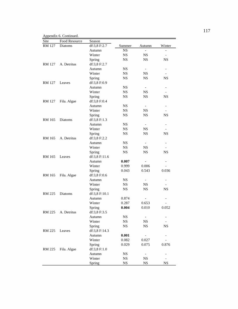
117
Appendix 6. Continued.
Site Food Resource SeasonRM 127 Diatoms df:3,8 F:2.7 Summer Autumn Winter
Autumn NS - -Winter NS NS -Spring NS NS NS
RM 127 A. Detritus df:3,8 F:2.7Autumn NS - -Winter NS NS -Spring NS NS NS
RM 127 Leaves df:3,8 F:0.9Autumn NS - -Winter NS NS -Spring NS NS NS
RM 127 Fila. Algae df:3,8 F:0.4Autumn NS - -Winter NS NS -Spring NS NS NS
RM 165 Diatoms df:3,8 F:1.3Autumn NS - -Winter NS NS -Spring NS NS NS
RM 165 A. Detritus df:3,8 F:2.2Autumn NS - -Winter NS NS -Spring NS NS NS
RM 165 Leaves df:3,8 F:11.6Autumn 0.007 - -Winter 0.999 0.006 -Spring 0.043 0.543 0.036
RM 165 Fila. Algae df:3,8 F:0.6Autumn NS - -Winter NS NS -Spring NS NS NS
RM 225 Diatoms df:3,8 F:10.1Autumn 0.874 - -Winter 0.287 0.653 -Spring 0.004 0.010 0.052
RM 225 A. Detritus df:3,8 F:3.5Autumn NS - -Winter NS NS -Spring NS NS NS
RM 225 Leaves df:3,8 F:14.3Autumn 0.001 - -Winter 0.082 0.027 -Spring 0.029 0.075 0.876
RM 225 Fila. Algae df:3,8 F:1.0Autumn NS - -Winter NS NS -Spring NS NS NS
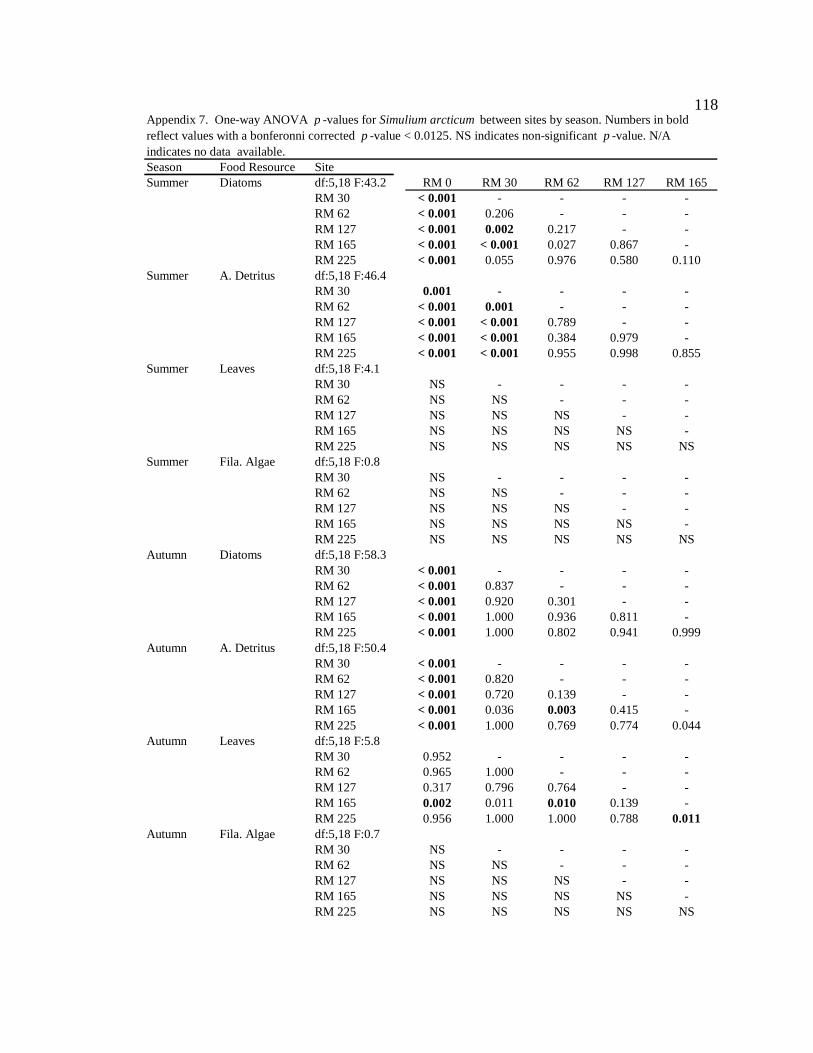
118
Season Food Resource SiteSummer Diatoms df:5,18 F:43.2 RM 0 RM 30 RM 62 RM 127 RM 165
RM 30 < 0.001 - - - -RM 62 < 0.001 0.206 - - -RM 127 < 0.001 0.002 0.217 - -RM 165 < 0.001 < 0.001 0.027 0.867 -RM 225 < 0.001 0.055 0.976 0.580 0.110
Summer A. Detritus df:5,18 F:46.4RM 30 0.001 - - - -RM 62 < 0.001 0.001 - - -RM 127 < 0.001 < 0.001 0.789 - -RM 165 < 0.001 < 0.001 0.384 0.979 -RM 225 < 0.001 < 0.001 0.955 0.998 0.855
Summer Leaves df:5,18 F:4.1RM 30 NS - - - -RM 62 NS NS - - -RM 127 NS NS NS - -RM 165 NS NS NS NS -RM 225 NS NS NS NS NS
Summer Fila. Algae df:5,18 F:0.8RM 30 NS - - - -RM 62 NS NS - - -RM 127 NS NS NS - -RM 165 NS NS NS NS -RM 225 NS NS NS NS NS
Autumn Diatoms df:5,18 F:58.3RM 30 < 0.001 - - - -RM 62 < 0.001 0.837 - - -RM 127 < 0.001 0.920 0.301 - -RM 165 < 0.001 1.000 0.936 0.811 -RM 225 < 0.001 1.000 0.802 0.941 0.999
Autumn A. Detritus df:5,18 F:50.4RM 30 < 0.001 - - - -RM 62 < 0.001 0.820 - - -RM 127 < 0.001 0.720 0.139 - -RM 165 < 0.001 0.036 0.003 0.415 -RM 225 < 0.001 1.000 0.769 0.774 0.044
Autumn Leaves df:5,18 F:5.8RM 30 0.952 - - - -RM 62 0.965 1.000 - - -RM 127 0.317 0.796 0.764 - -RM 165 0.002 0.011 0.010 0.139 -RM 225 0.956 1.000 1.000 0.788 0.011
Autumn Fila. Algae df:5,18 F:0.7RM 30 NS - - - -RM 62 NS NS - - -RM 127 NS NS NS - -RM 165 NS NS NS NS -RM 225 NS NS NS NS NS
Appendix 7. One-way ANOVA p -values for Simulium arcticum between sites by season. Numbers in bold reflect values with a bonferonni corrected p -value < 0.0125. NS indicates non-significant p -value. N/A indicates no data available.
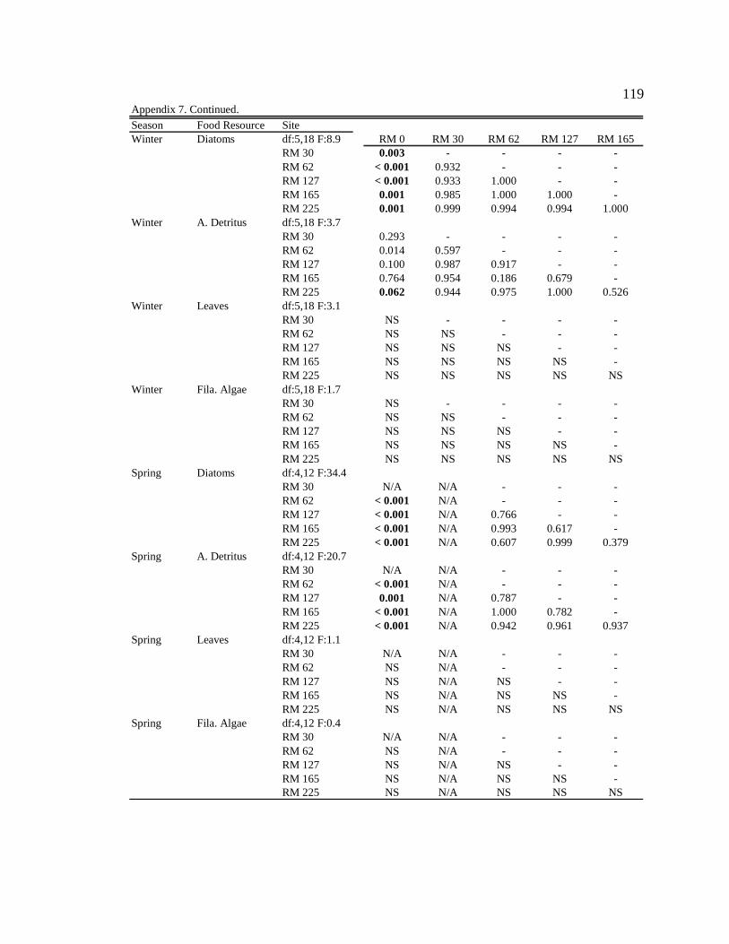
119
Appendix 7. Continued.
Season Food Resource SiteWinter Diatoms df:5,18 F:8.9 RM 0 RM 30 RM 62 RM 127 RM 165
RM 30 0.003 - - - -RM 62 < 0.001 0.932 - - -RM 127 < 0.001 0.933 1.000 - -RM 165 0.001 0.985 1.000 1.000 -RM 225 0.001 0.999 0.994 0.994 1.000
Winter A. Detritus df:5,18 F:3.7RM 30 0.293 - - - -RM 62 0.014 0.597 - - -RM 127 0.100 0.987 0.917 - -RM 165 0.764 0.954 0.186 0.679 -RM 225 0.062 0.944 0.975 1.000 0.526
Winter Leaves df:5,18 F:3.1RM 30 NS - - - -RM 62 NS NS - - -RM 127 NS NS NS - -RM 165 NS NS NS NS -RM 225 NS NS NS NS NS
Winter Fila. Algae df:5,18 F:1.7RM 30 NS - - - -RM 62 NS NS - - -RM 127 NS NS NS - -RM 165 NS NS NS NS -RM 225 NS NS NS NS NS
Spring Diatoms df:4,12 F:34.4RM 30 N/A N/A - - -RM 62 < 0.001 N/A - - -RM 127 < 0.001 N/A 0.766 - -RM 165 < 0.001 N/A 0.993 0.617 -RM 225 < 0.001 N/A 0.607 0.999 0.379
Spring A. Detritus df:4,12 F:20.7RM 30 N/A N/A - - -RM 62 < 0.001 N/A - - -RM 127 0.001 N/A 0.787 - -RM 165 < 0.001 N/A 1.000 0.782 -RM 225 < 0.001 N/A 0.942 0.961 0.937
Spring Leaves df:4,12 F:1.1RM 30 N/A N/A - - -RM 62 NS N/A - - -RM 127 NS N/A NS - -RM 165 NS N/A NS NS -RM 225 NS N/A NS NS NS
Spring Fila. Algae df:4,12 F:0.4RM 30 N/A N/A - - -RM 62 NS N/A - - -RM 127 NS N/A NS - -RM 165 NS N/A NS NS -RM 225 NS N/A NS NS NS
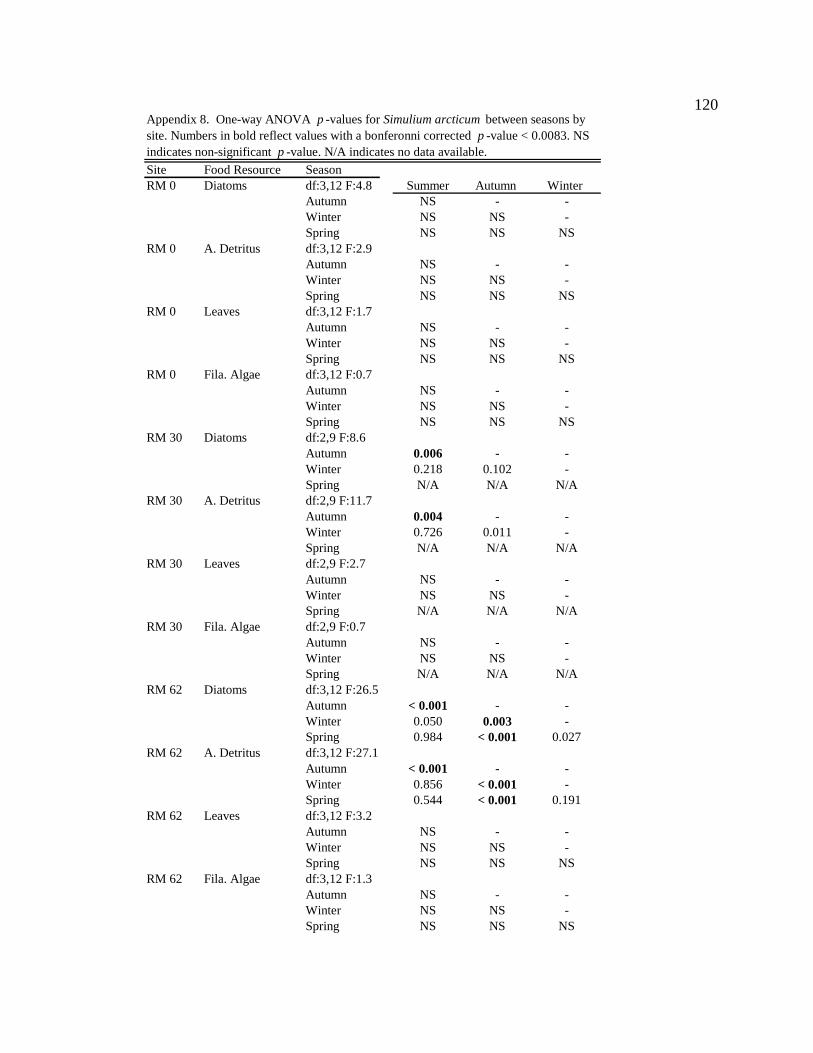
120
Site Food Resource SeasonRM 0 Diatoms df:3,12 F:4.8 Summer Autumn Winter
Autumn NS - -Winter NS NS -Spring NS NS NS
RM 0 A. Detritus df:3,12 F:2.9Autumn NS - -Winter NS NS -Spring NS NS NS
RM 0 Leaves df:3,12 F:1.7Autumn NS - -Winter NS NS -Spring NS NS NS
RM 0 Fila. Algae df:3,12 F:0.7Autumn NS - -Winter NS NS -Spring NS NS NS
RM 30 Diatoms df:2,9 F:8.6Autumn 0.006 - -Winter 0.218 0.102 -Spring N/A N/A N/A
RM 30 A. Detritus df:2,9 F:11.7Autumn 0.004 - -Winter 0.726 0.011 -Spring N/A N/A N/A
RM 30 Leaves df:2,9 F:2.7Autumn NS - -Winter NS NS -Spring N/A N/A N/A
RM 30 Fila. Algae df:2,9 F:0.7Autumn NS - -Winter NS NS -Spring N/A N/A N/A
RM 62 Diatoms df:3,12 F:26.5Autumn < 0.001 - -Winter 0.050 0.003 -Spring 0.984 < 0.001 0.027
RM 62 A. Detritus df:3,12 F:27.1Autumn < 0.001 - -Winter 0.856 < 0.001 -Spring 0.544 < 0.001 0.191
RM 62 Leaves df:3,12 F:3.2Autumn NS - -Winter NS NS -Spring NS NS NS
RM 62 Fila. Algae df:3,12 F:1.3Autumn NS - -Winter NS NS -Spring NS NS NS
Appendix 8. One-way ANOVA p -values for Simulium arcticum between seasons by site. Numbers in bold reflect values with a bonferonni corrected p -value < 0.0083. NS indicates non-significant p-value. N/A indicates no data available.
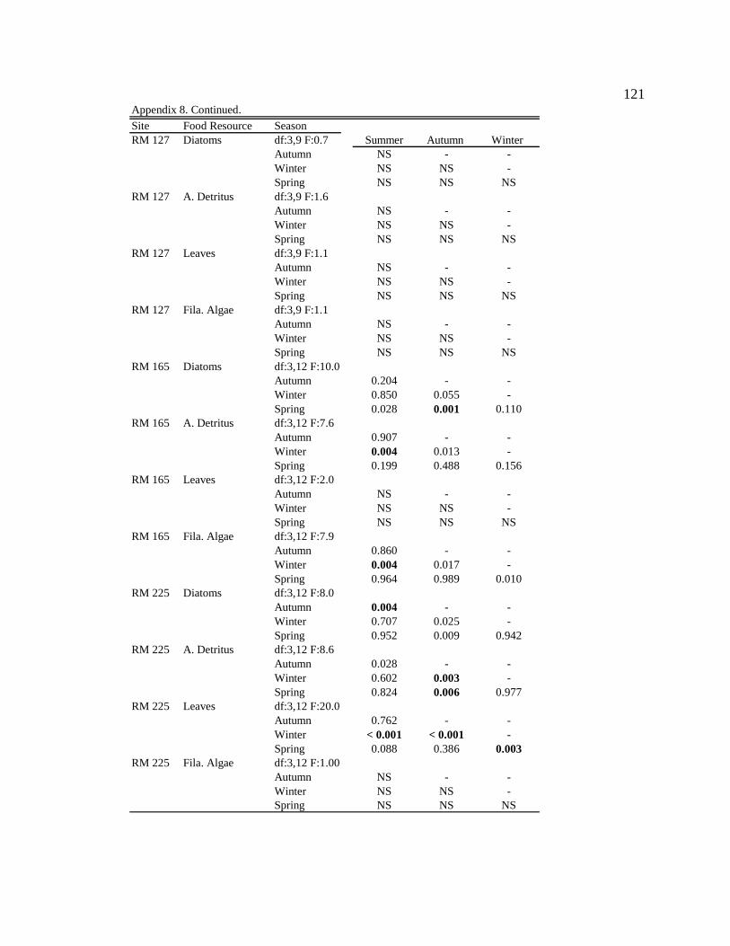
121
Appendix 8. Continued.
Site Food Resource SeasonRM 127 Diatoms df:3,9 F:0.7 Summer Autumn Winter
Autumn NS - -Winter NS NS -Spring NS NS NS
RM 127 A. Detritus df:3,9 F:1.6Autumn NS - -Winter NS NS -Spring NS NS NS
RM 127 Leaves df:3,9 F:1.1Autumn NS - -Winter NS NS -Spring NS NS NS
RM 127 Fila. Algae df:3,9 F:1.1Autumn NS - -Winter NS NS -Spring NS NS NS
RM 165 Diatoms df:3,12 F:10.0Autumn 0.204 - -Winter 0.850 0.055 -Spring 0.028 0.001 0.110
RM 165 A. Detritus df:3,12 F:7.6Autumn 0.907 - -Winter 0.004 0.013 -Spring 0.199 0.488 0.156
RM 165 Leaves df:3,12 F:2.0Autumn NS - -Winter NS NS -Spring NS NS NS
RM 165 Fila. Algae df:3,12 F:7.9Autumn 0.860 - -Winter 0.004 0.017 -Spring 0.964 0.989 0.010
RM 225 Diatoms df:3,12 F:8.0Autumn 0.004 - -Winter 0.707 0.025 -Spring 0.952 0.009 0.942
RM 225 A. Detritus df:3,12 F:8.6Autumn 0.028 - -Winter 0.602 0.003 -Spring 0.824 0.006 0.977
RM 225 Leaves df:3,12 F:20.0Autumn 0.762 - -Winter < 0.001 < 0.001 -Spring 0.088 0.386 0.003
RM 225 Fila. Algae df:3,12 F:1.00Autumn NS - -Winter NS NS -Spring NS NS NS

122
Season Food Resource SiteSummer Diatoms df:4,10 F:2.4 RM 0 RM 30 RM 62 RM 127 RM 165
RM 30 NS - - - -RM 62 NS NS - - -RM 127 NS NS NS - -RM 165 N/A N/A N/A N/A -RM 225 NS NS NS NS N/A
Summer A. Detritus df:4,10 F:0.7RM 30 NS - - - -RM 62 NS NS - - -RM 127 NS NS NS - -RM 165 N/A N/A N/A N/A -RM 225 NS NS NS NS N/A
Summer Leaves df:4,10 F:0.1RM 30 NS - - - -RM 62 NS NS - - -RM 127 NS NS NS - -RM 165 N/A N/A N/A N/A -RM 225 NS NS NS NS N/A
Summer Fila. Algae df:4,10 F:0.8RM 30 NS - - - -RM 62 NS NS - - -RM 127 NS NS NS - -RM 165 N/A N/A N/A N/A -RM 225 NS NS NS NS N/A
Autumn Diatoms df:5,18 F:30.5RM 30 0.002 - - - -RM 62 < 0.001 < 0.001 - - -RM 127 < 0.001 0.005 0.650 - -RM 165 < 0.001 0.253 0.023 0.359 -RM 225 < 0.001 0.002 0.871 0.998 0.188
Autumn A. Detritus df:5,18 F:6.5RM 30 0.166 - - - -RM 62 0.010 0.714 - - -RM 127 0.277 1.000 0.526 - -RM 165 0.542 0.959 0.266 0.995 -RM 225 0.001 0.126 0.797 0.07 0.025
Autumn Leaves df:5,18 F:6.2RM 30 0.009 - - - -RM 62 0.025 0.997 - - -RM 127 0.015 1.000 1.000 - -RM 165 0.001 0.877 0.636 0.780 -RM 225 0.273 0.513 0.781 0.637 0.093
Autumn Fila. Algae df:5,18 F:1.6RM 30 NS - - - -RM 62 NS NS - - -RM 127 NS NS NS - -RM 165 NS NS NS NS -RM 225 NS NS NS NS NS
Appendix 9. One-way ANOVA p -values for Gammarus lacustrisbetween sites by season. Numbers in bold reflect values with a bonferonni corrected p -value < 0.0125. NS indicates non-significant p -value. N/A indicates no data available.
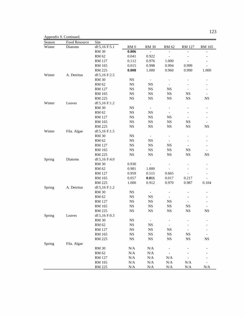
123
Appendix 9. Continued.
Season Food Resource SiteWinter Diatoms df:5,16 F:5.1 RM 0 RM 30 RM 62 RM 127 RM 165
RM 30 0.006 - - - -RM 62 0.041 0.922 - - -RM 127 0.112 0.976 1.000 - -RM 165 0.015 0.998 0.994 0.999 -RM 225 0.008 1.000 0.960 0.990 1.000
Winter A. Detritus df:5,16 F:2.5RM 30 NS - - - -RM 62 NS NS - - -RM 127 NS NS NS - -RM 165 NS NS NS NS -RM 225 NS NS NS NS NS
Winter Leaves df:5,16 F:1.2RM 30 NS - - - -RM 62 NS NS - - -RM 127 NS NS NS - -RM 165 NS NS NS NS -RM 225 NS NS NS NS NS
Winter Fila. Algae df:5,16 F:1.5RM 30 NS - - - -RM 62 NS NS - - -RM 127 NS NS NS - -RM 165 NS NS NS NS -RM 225 NS NS NS NS NS
Spring Diatoms df:5,16 F:4.0RM 30 0.930 - - - -RM 62 0.981 1.000 - - -RM 127 0.959 0.515 0.665 - -RM 165 0.057 0.011 0.017 0.217 -RM 225 1.000 0.912 0.970 0.987 0.104
Spring A. Detritus df:5,16 F:1.2RM 30 NS - - - -RM 62 NS NS - - -RM 127 NS NS NS - -RM 165 NS NS NS NS -RM 225 NS NS NS NS NS
Spring Leaves df:5,16 F:0.3RM 30 NS - - - -RM 62 NS NS - - -RM 127 NS NS NS - -RM 165 NS NS NS NS -RM 225 NS NS NS NS NS
Spring Fila. AlgaeRM 30 N/A N/A - - -RM 62 N/A N/A - - -RM 127 N/A N/A N/A - -RM 165 N/A N/A N/A N/A -RM 225 N/A N/A N/A N/A N/A
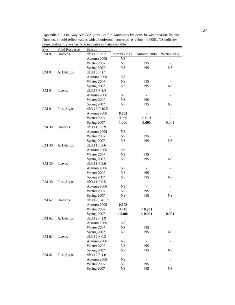
124
Site Food Resource SeasonRM 0 Diatoms df:3,13 F:0.2 Summer 2006 Autumn 2006 Winter 2007
Autumn 2006 NS - -Winter 2007 NS NS -Spring 2007 NS NS NS
RM 0 A. Detritus df:3,13 F:1.7Autumn 2006 NS - -Winter 2007 NS NS -Spring 2007 NS NS NS
RM 0 Leaves df:3,13 F:1.4Autumn 2006 NS - -Winter 2007 NS NS -Spring 2007 NS NS NS
RM 0 Fila. Algae df:3,13 F:10.5Autumn 2006 0.002 - -Winter 2007 0.030 0.519 -Spring 2007 1.000 0.003 0.041
RM 30 Diatoms df:3,11 F:5.9Autumn 2006 NS - -Winter 2007 NS NS -Spring 2007 NS NS NS
RM 30 A. Detritus df:3,11 F:2.6Autumn 2006 NS - -Winter 2007 NS NS -Spring 2007 NS NS NS
RM 30 Leaves df:3,11 F:2.6Autumn 2006 NS - -Winter 2007 NS NS -Spring 2007 NS NS NS
RM 30 Fila. Algae df:3,11 F:0.5Autumn 2006 NS - -Winter 2007 NS NS -Spring 2007 NS NS NS
RM 62 Diatoms df:3,12 F:41.7Autumn 2006 0.003 - -Winter 2007 0.718 < 0.001 -Spring 2007 < 0.001 < 0.001 0.001
RM 62 A. Detritus df:3,12 F:1.9Autumn 2006 NS - -Winter 2007 NS NS -Spring 2007 NS NS NS
RM 62 Leaves df:3,12 F:0.2Autumn 2006 NS - -Winter 2007 NS NS -Spring 2007 NS NS NS
RM 62 Fila. Algae df:3,12 F:1.0Autumn 2006 NS - -Winter 2007 NS NS -Spring 2007 NS NS NS
Appendix 10. One-way ANOVA p-values for Gammarus lacustris between seasons by site. Numbers in bold reflect values with a bonferonni corrected p -value < 0.0083. NS indicates non-significant p -value. N/A indicates no data available.

125
Appendix 10. Continued.
Site Food Resource SeasonRM 127 Diatoms df:3,7 F:4.4 Summer Autumn Winter
Autumn NS - -Winter NS NS -Spring NS NS NS
RM 127 A. Detritus df:3,7 F:1.3Autumn NS - -Winter NS NS -Spring NS NS NS
RM 127 Leaves df:3,7 F:7.2Autumn NS - -Winter NS NS -Spring NS NS NS
RM 127 Fila. Algae df:3,7 F:63.2Autumn 0.466 - -Winter < 0.001 < 0.001 -Spring 1.000 0.158 < 0.001
RM 165 Diatoms df:2,8 F:2.6Autumn N/A - -Winter N/A NS -Spring N/A NS NS
RM 165 A. Detritus df:2,8 F:0.3Autumn N/A - -Winter N/A NS -Spring N/A NS NS
RM 165 Leaves df:2,8 F:7.2Autumn N/A - -Winter N/A NS -Spring N/A NS NS
RM 165 Fila. Algae df:2,8 F:1.6Autumn N/A - -Winter N/A NS -Spring N/A NS NS
RM 225 Diatoms df:3,9 F:13.4Autumn 0.037 - -Winter 0.729 0.081 -Spring 0.233 0.001 0.022
RM 225 A. Detritus df:3,9 F:9.4Autumn 0.422 - -Winter 0.752 0.045 -Spring 0.078 0.003 0.184
RM 225 Leaves df:3,9 F:1.1Autumn NS - -Winter NS NS -Spring NS NS NS
RM 225 Fila. Algae df:3,9 F:3.2Autumn NS - -Winter NS NS -Spring NS NS NS
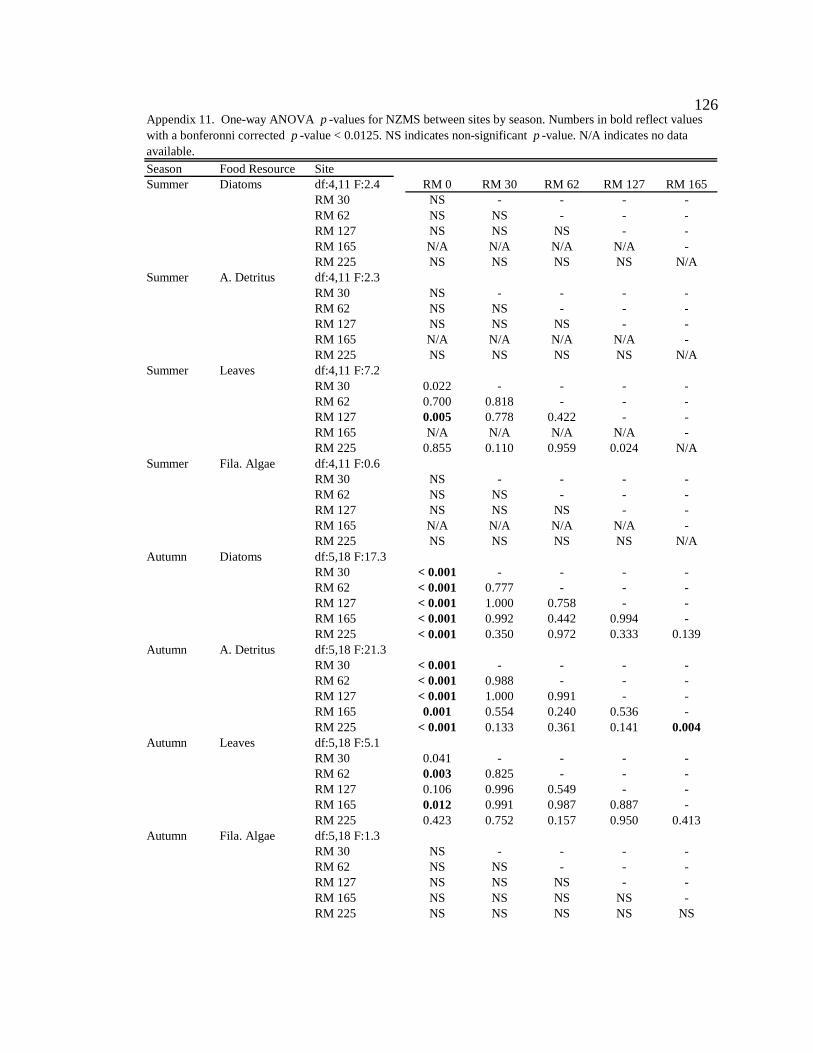
126
Season Food Resource SiteSummer Diatoms df:4,11 F:2.4 RM 0 RM 30 RM 62 RM 127 RM 165
RM 30 NS - - - -RM 62 NS NS - - -RM 127 NS NS NS - -RM 165 N/A N/A N/A N/A -RM 225 NS NS NS NS N/A
Summer A. Detritus df:4,11 F:2.3RM 30 NS - - - -RM 62 NS NS - - -RM 127 NS NS NS - -RM 165 N/A N/A N/A N/A -RM 225 NS NS NS NS N/A
Summer Leaves df:4,11 F:7.2RM 30 0.022 - - - -RM 62 0.700 0.818 - - -RM 127 0.005 0.778 0.422 - -RM 165 N/A N/A N/A N/A -RM 225 0.855 0.110 0.959 0.024 N/A
Summer Fila. Algae df:4,11 F:0.6RM 30 NS - - - -RM 62 NS NS - - -RM 127 NS NS NS - -RM 165 N/A N/A N/A N/A -RM 225 NS NS NS NS N/A
Autumn Diatoms df:5,18 F:17.3RM 30 < 0.001 - - - -RM 62 < 0.001 0.777 - - -RM 127 < 0.001 1.000 0.758 - -RM 165 < 0.001 0.992 0.442 0.994 -RM 225 < 0.001 0.350 0.972 0.333 0.139
Autumn A. Detritus df:5,18 F:21.3RM 30 < 0.001 - - - -RM 62 < 0.001 0.988 - - -RM 127 < 0.001 1.000 0.991 - -RM 165 0.001 0.554 0.240 0.536 -RM 225 < 0.001 0.133 0.361 0.141 0.004
Autumn Leaves df:5,18 F:5.1RM 30 0.041 - - - -RM 62 0.003 0.825 - - -RM 127 0.106 0.996 0.549 - -RM 165 0.012 0.991 0.987 0.887 -RM 225 0.423 0.752 0.157 0.950 0.413
Autumn Fila. Algae df:5,18 F:1.3RM 30 NS - - - -RM 62 NS NS - - -RM 127 NS NS NS - -RM 165 NS NS NS NS -RM 225 NS NS NS NS NS
Appendix 11. One-way ANOVA p -values for NZMS between sites by season. Numbers in bold reflect values with a bonferonni corrected p-value < 0.0125. NS indicates non-significant p-value. N/A indicates no data available.
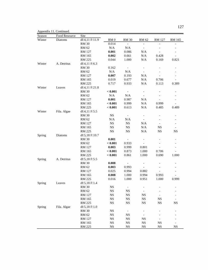
127
Appendix 11. Continued.
Season Food Resource SiteWinter Diatoms df:4,11 F:11.9 RM 0 RM 30 RM 62 RM 127 RM 165
RM 30 0.014 - - - -RM 62 N/A N/A - - -RM 127 0.001 0.086 N/A - -RM 165 0.002 0.661 N/A 0.428 -RM 225 0.044 1.000 N/A 0.169 0.821
Winter A. Detritus df:4,11 F:6.3RM 30 0.162 - - - -RM 62 N/A N/A - - -RM 127 0.007 0.193 N/A - -RM 165 0.019 0.677 N/A 0.706 -RM 225 0.717 0.933 N/A 0.113 0.389
Winter Leaves df:4,11 F:21.8RM 30 < 0.001 - - - -RM 62 N/A N/A - - -RM 127 0.001 0.987 N/A - -RM 165 < 0.001 0.999 N/A 0.999 -RM 225 < 0.001 0.613 N/A 0.485 0.489
Winter Fila. Algae df:4,11 F:5.5RM 30 NS - - - -RM 62 N/A N/A - - -RM 127 NS NS N/A - -RM 165 NS NS N/A NS -RM 225 NS NS N/A NS NS
Spring Diatoms df:5,18 F:10.7RM 30 0.001 - - - -RM 62 < 0.001 0.933 - - -RM 127 0.003 0.999 0.801 - -RM 165 < 0.001 0.873 1.000 0.706 -RM 225 < 0.001 0.861 1.000 0.690 1.000
Spring A. Detritus df:5,18 F:5.5RM 30 0.008 - - - -RM 62 0.003 0.993 - - -RM 127 0.025 0.994 0.882 - -RM 165 0.008 1.000 0.994 0.993 -RM 225 0.016 1.000 0.951 1.000 0.999
Spring Leaves df:5,18 F:1.4RM 30 NS - - - -RM 62 NS NS - - -RM 127 NS NS NS - -RM 165 NS NS NS NS -RM 225 NS NS NS NS NS
Spring Fila. Algae df:5,18 F:1.0RM 30 NS - - - -RM 62 NS NS - - -RM 127 NS NS NS - -RM 165 NS NS NS NS -RM 225 NS NS NS NS NS

128
Site Food Resource SeasonRM 0 Diatoms df:3,12 F:0.6 Summer Autumn Winter
Autumn NS - -Winter NS NS -Spring NS NS NS
RM 0 A. Detritus df:3,12 F:0.6Autumn NS - -Winter NS NS -Spring NS NS NS
RM 0 Leaves df:3,12 F:12.2Autumn 0.005 - -Winter 0.106 0.320 -Spring < 0.001 0.517 0.033
RM 0 Fila. Algae df:3,12 F:0.7Autumn NS - -Winter NS NS -Spring NS NS NS
RM 30 Diatoms df:3,12 F:1.1Autumn NS - -Winter NS NS -Spring NS NS NS
RM 30 A. Detritus df:3,12 F:10.9Autumn 0.015 - -Winter 0.964 0.007 -Spring 0.009 0.989 0.004
RM 30 Leaves df:3,12 F:7.7Autumn 0.196 - -Winter 0.461 0.015 -Spring 0.072 0.925 0.005
RM 30 Fila. AlgaeAutumn N/A - -Winter N/A N/A -Spring N/A N/A N/A
RM 62 Diatoms df:2,6 F:0.1Autumn NS - -Winter N/A N/A -Spring NS NS N/A
RM 62 A. Detritus df:2,6 F:0.5Autumn NS - -Winter N/A N/A -Spring NS NS N/A
RM 62 Leaves df:2,6 F:3.1Autumn NS - -Winter N/A N/A -Spring NS NS N/A
RM 62 Fila. Algae df:2,6 F:0.5Autumn NS - -Winter N/A N/A -Spring NS NS N/A
Appendix 12. One-way ANOVA p -values for NZMS between seasons by site. Numbers in bold reflect values with a bonferonni corrected p-value < 0.0083. NS indicates non-significant p-value. N/A indicates no data available.
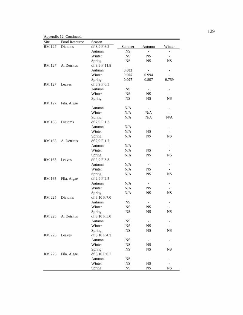
129
Appendix 12. Continued.
Site Food Resource SeasonRM 127 Diatoms df:3,9 F:6.2 Summer Autumn Winter
Autumn NS - -Winter NS NS -Spring NS NS NS
RM 127 A. Detritus df:3,9 F:11.8Autumn 0.002 - -Winter 0.005 0.994 -Spring 0.007 0.807 0.759
RM 127 Leaves df:3,9 F:6.3Autumn NS - -Winter NS NS -Spring NS NS NS
RM 127 Fila. AlgaeAutumn N/A - -Winter N/A N/A -Spring N/A N/A N/A
RM 165 Diatoms df:2,9 F:1.3Autumn N/A - -Winter N/A NS -Spring N/A NS NS
RM 165 A. Detritus df:2,9 F:1.7Autumn N/A - -Winter N/A NS -Spring N/A NS NS
RM 165 Leaves df:2,9 F:3.8Autumn N/A - -Winter N/A NS -Spring N/A NS NS
RM 165 Fila. Algae df:2,9 F:2.5Autumn N/A - -Winter N/A NS -Spring N/A NS NS
RM 225 Diatoms df:3,10 F:7.0Autumn NS - -Winter NS NS -Spring NS NS NS
RM 225 A. Detritus df:3,10 F:5.0Autumn NS - -Winter NS NS -Spring NS NS NS
RM 225 Leaves df:3,10 F:4.2Autumn NS - -Winter NS NS -Spring NS NS NS
RM 225 Fila. Algae df:3,10 F:0.7Autumn NS - -Winter NS NS -Spring NS NS NS
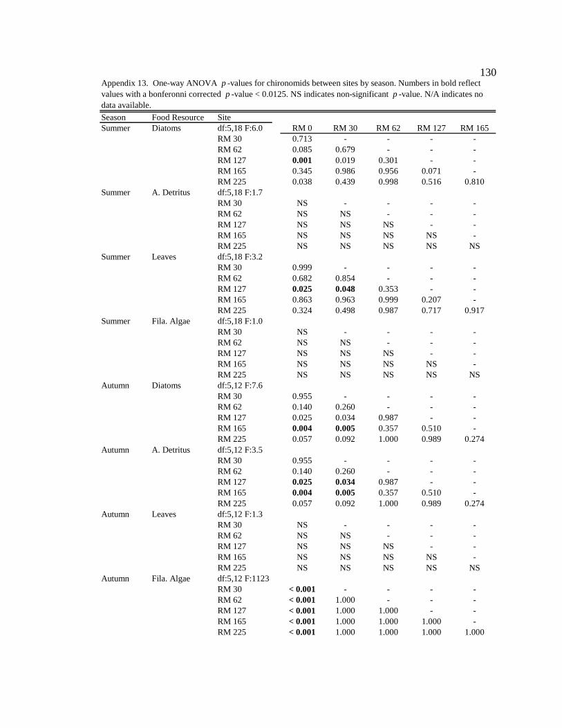
130
Season Food Resource SiteSummer Diatoms df:5,18 F:6.0 RM 0 RM 30 RM 62 RM 127 RM 165
RM 30 0.713 - - - -RM 62 0.085 0.679 - - -RM 127 0.001 0.019 0.301 - -RM 165 0.345 0.986 0.956 0.071 -RM 225 0.038 0.439 0.998 0.516 0.810
Summer A. Detritus df:5,18 F:1.7RM 30 NS - - - -RM 62 NS NS - - -RM 127 NS NS NS - -RM 165 NS NS NS NS -RM 225 NS NS NS NS NS
Summer Leaves df:5,18 F:3.2RM 30 0.999 - - - -RM 62 0.682 0.854 - - -RM 127 0.025 0.048 0.353 - -RM 165 0.863 0.963 0.999 0.207 -RM 225 0.324 0.498 0.987 0.717 0.917
Summer Fila. Algae df:5,18 F:1.0RM 30 NS - - - -RM 62 NS NS - - -RM 127 NS NS NS - -RM 165 NS NS NS NS -RM 225 NS NS NS NS NS
Autumn Diatoms df:5,12 F:7.6RM 30 0.955 - - - -RM 62 0.140 0.260 - - -RM 127 0.025 0.034 0.987 - -RM 165 0.004 0.005 0.357 0.510 -RM 225 0.057 0.092 1.000 0.989 0.274
Autumn A. Detritus df:5,12 F:3.5RM 30 0.955 - - - -RM 62 0.140 0.260 - - -RM 127 0.025 0.034 0.987 - -RM 165 0.004 0.005 0.357 0.510 -RM 225 0.057 0.092 1.000 0.989 0.274
Autumn Leaves df:5,12 F:1.3RM 30 NS - - - -RM 62 NS NS - - -RM 127 NS NS NS - -RM 165 NS NS NS NS -RM 225 NS NS NS NS NS
Autumn Fila. Algae df:5,12 F:1123RM 30 < 0.001 - - - -RM 62 < 0.001 1.000 - - -RM 127 < 0.001 1.000 1.000 - -RM 165 < 0.001 1.000 1.000 1.000 -RM 225 < 0.001 1.000 1.000 1.000 1.000
Appendix 13. One-way ANOVA p -values for chironomids between sites by season. Numbers in bold reflect values with a bonferonni corrected p -value < 0.0125. NS indicates non-significant p -value. N/A indicates no data available.
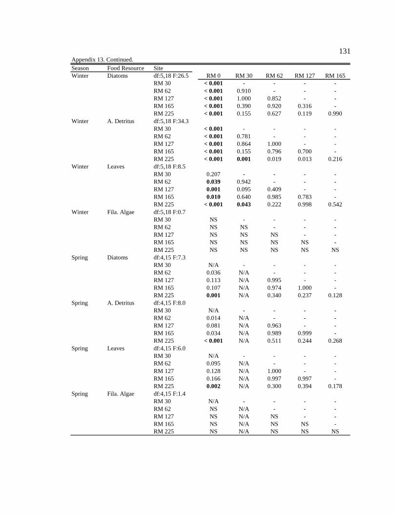
131
Appendix 13. Continued.
Season Food Resource SiteWinter Diatoms df:5,18 F:26.5 RM 0 RM 30 RM 62 RM 127 RM 165
RM 30 < 0.001 - - - -RM 62 < 0.001 0.910 - - -RM 127 < 0.001 1.000 0.852 - -RM 165 < 0.001 0.390 0.920 0.316 -RM 225 < 0.001 0.155 0.627 0.119 0.990
Winter A. Detritus df:5,18 F:34.3RM 30 < 0.001 - - - -RM 62 < 0.001 0.781 - - -RM 127 < 0.001 0.864 1.000 - -RM 165 < 0.001 0.155 0.796 0.700 -RM 225 < 0.001 0.001 0.019 0.013 0.216
Winter Leaves df:5,18 F:8.5RM 30 0.207 - - - -RM 62 0.039 0.942 - - -RM 127 0.001 0.095 0.409 - -RM 165 0.010 0.640 0.985 0.783 -RM 225 < 0.001 0.043 0.222 0.998 0.542
Winter Fila. Algae df:5,18 F:0.7RM 30 NS - - - -RM 62 NS NS - - -RM 127 NS NS NS - -RM 165 NS NS NS NS -RM 225 NS NS NS NS NS
Spring Diatoms df:4,15 F:7.3RM 30 N/A - - - -RM 62 0.036 N/A - - -RM 127 0.113 N/A 0.995 - -RM 165 0.107 N/A 0.974 1.000 -RM 225 0.001 N/A 0.340 0.237 0.128
Spring A. Detritus df:4,15 F:8.0RM 30 N/A - - - -RM 62 0.014 N/A - - -RM 127 0.081 N/A 0.963 - -RM 165 0.034 N/A 0.989 0.999 -RM 225 < 0.001 N/A 0.511 0.244 0.268
Spring Leaves df:4,15 F:6.0RM 30 N/A - - - -RM 62 0.095 N/A - - -RM 127 0.128 N/A 1.000 - -RM 165 0.166 N/A 0.997 0.997 -RM 225 0.002 N/A 0.300 0.394 0.178
Spring Fila. Algae df:4,15 F:1.4RM 30 N/A - - - -RM 62 NS N/A - - -RM 127 NS N/A NS - -RM 165 NS N/A NS NS -RM 225 NS N/A NS NS NS
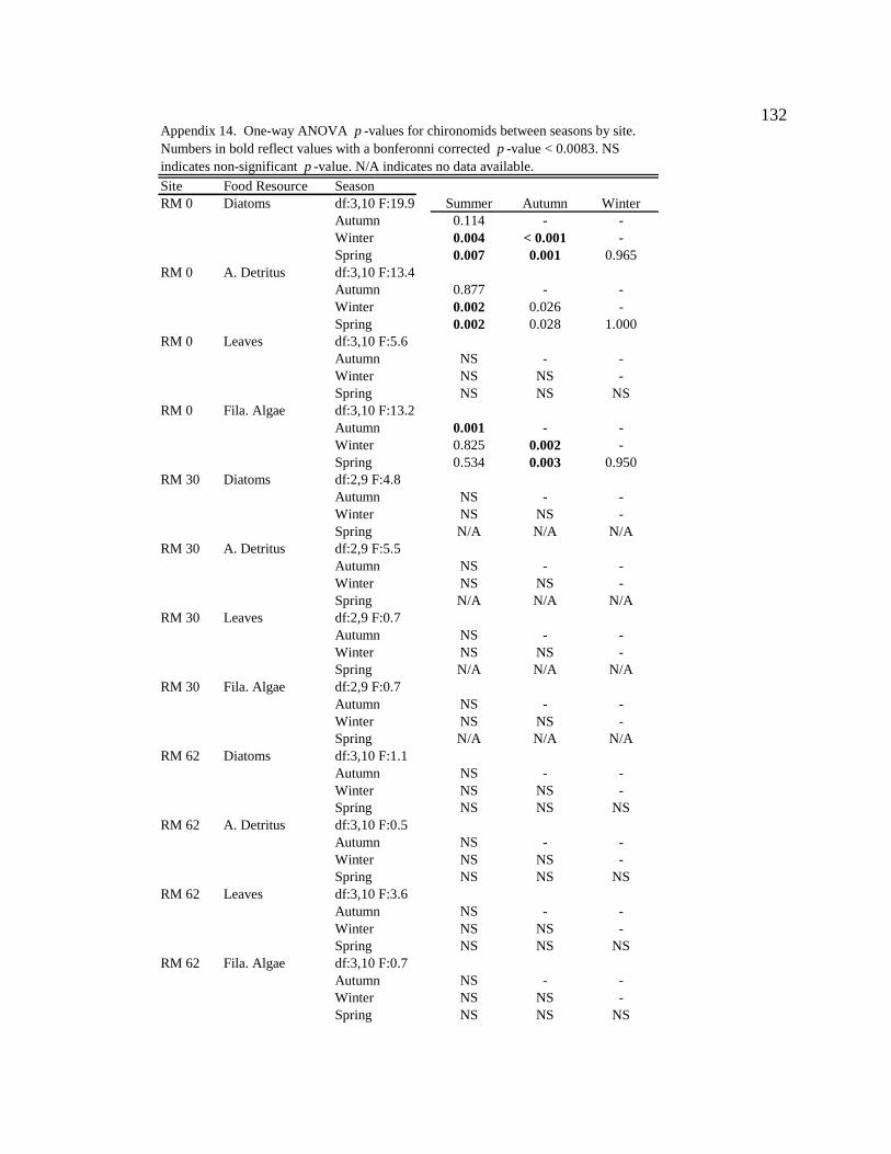
132
Site Food Resource SeasonRM 0 Diatoms df:3,10 F:19.9 Summer Autumn Winter
Autumn 0.114 - -Winter 0.004 < 0.001 -Spring 0.007 0.001 0.965
RM 0 A. Detritus df:3,10 F:13.4Autumn 0.877 - -Winter 0.002 0.026 -Spring 0.002 0.028 1.000
RM 0 Leaves df:3,10 F:5.6Autumn NS - -Winter NS NS -Spring NS NS NS
RM 0 Fila. Algae df:3,10 F:13.2Autumn 0.001 - -Winter 0.825 0.002 -Spring 0.534 0.003 0.950
RM 30 Diatoms df:2,9 F:4.8Autumn NS - -Winter NS NS -Spring N/A N/A N/A
RM 30 A. Detritus df:2,9 F:5.5Autumn NS - -Winter NS NS -Spring N/A N/A N/A
RM 30 Leaves df:2,9 F:0.7Autumn NS - -Winter NS NS -Spring N/A N/A N/A
RM 30 Fila. Algae df:2,9 F:0.7Autumn NS - -Winter NS NS -Spring N/A N/A N/A
RM 62 Diatoms df:3,10 F:1.1Autumn NS - -Winter NS NS -Spring NS NS NS
RM 62 A. Detritus df:3,10 F:0.5Autumn NS - -Winter NS NS -Spring NS NS NS
RM 62 Leaves df:3,10 F:3.6Autumn NS - -Winter NS NS -Spring NS NS NS
RM 62 Fila. Algae df:3,10 F:0.7Autumn NS - -Winter NS NS -Spring NS NS NS
Appendix 14. One-way ANOVA p -values for chironomids between seasons by site. Numbers in bold reflect values with a bonferonni corrected p -value < 0.0083. NS indicates non-significant p-value. N/A indicates no data available.
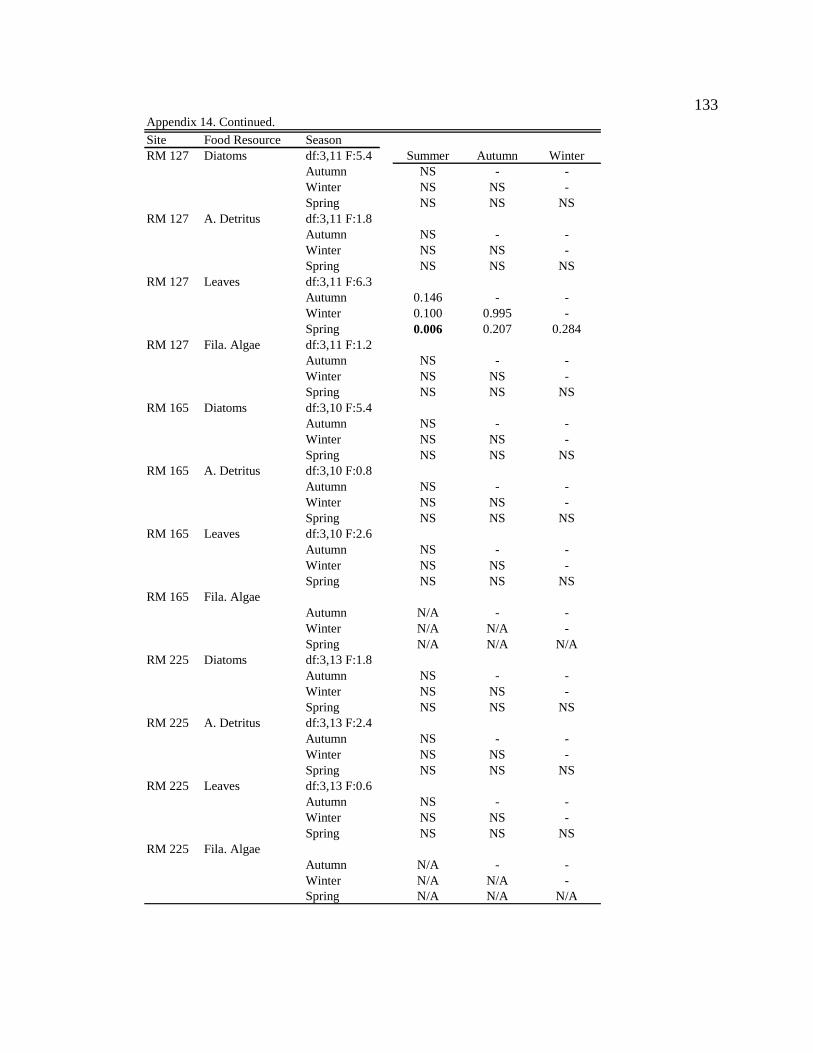
133
Appendix 14. Continued.
Site Food Resource SeasonRM 127 Diatoms df:3,11 F:5.4 Summer Autumn Winter
Autumn NS - -Winter NS NS -Spring NS NS NS
RM 127 A. Detritus df:3,11 F:1.8Autumn NS - -Winter NS NS -Spring NS NS NS
RM 127 Leaves df:3,11 F:6.3Autumn 0.146 - -Winter 0.100 0.995 -Spring 0.006 0.207 0.284
RM 127 Fila. Algae df:3,11 F:1.2Autumn NS - -Winter NS NS -Spring NS NS NS
RM 165 Diatoms df:3,10 F:5.4Autumn NS - -Winter NS NS -Spring NS NS NS
RM 165 A. Detritus df:3,10 F:0.8Autumn NS - -Winter NS NS -Spring NS NS NS
RM 165 Leaves df:3,10 F:2.6Autumn NS - -Winter NS NS -Spring NS NS NS
RM 165 Fila. AlgaeAutumn N/A - -Winter N/A N/A -Spring N/A N/A N/A
RM 225 Diatoms df:3,13 F:1.8Autumn NS - -Winter NS NS -Spring NS NS NS
RM 225 A. Detritus df:3,13 F:2.4Autumn NS - -Winter NS NS -Spring NS NS NS
RM 225 Leaves df:3,13 F:0.6Autumn NS - -Winter NS NS -Spring NS NS NS
RM 225 Fila. AlgaeAutumn N/A - -Winter N/A N/A -Spring N/A N/A N/A

134
APPENDIX B
ALGAL COMMUNITY COMPOSITION TABLES
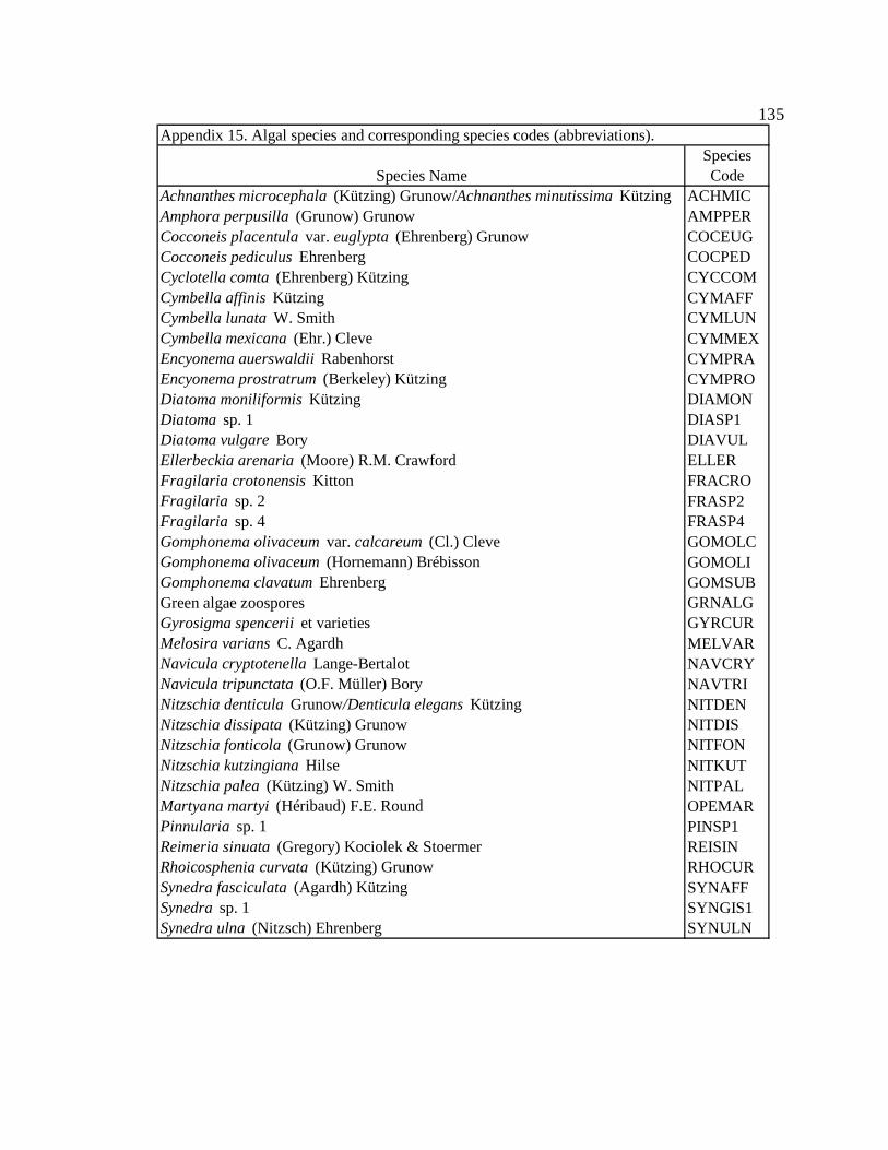
135Appendix 15. Algal species and corresponding species codes (abbreviations).
Species NameSpecies Code
Achnanthes microcephala (Kützing) Grunow/Achnanthes minutissima Kützing ACHMICAmphora perpusilla (Grunow) Grunow AMPPERCocconeis placentula var. euglypta (Ehrenberg) Grunow COCEUGCocconeis pediculus Ehrenberg COCPEDCyclotella comta (Ehrenberg) Kützing CYCCOMCymbella affinis Kützing CYMAFFCymbella lunata W. Smith CYMLUNCymbella mexicana (Ehr.) Cleve CYMMEXEncyonema auerswaldii Rabenhorst CYMPRAEncyonema prostratrum (Berkeley) Kützing CYMPRODiatoma moniliformis Kützing DIAMONDiatoma sp. 1 DIASP1Diatoma vulgare Bory DIAVULEllerbeckia arenaria (Moore) R.M. Crawford ELLERFragilaria crotonensis Kitton FRACROFragilaria sp. 2 FRASP2Fragilaria sp. 4 FRASP4Gomphonema olivaceum var. calcareum (Cl.) Cleve GOMOLCGomphonema olivaceum (Hornemann) Brébisson GOMOLIGomphonema clavatum Ehrenberg GOMSUBGreen algae zoospores GRNALGGyrosigma spencerii et varieties GYRCURMelosira varians C. Agardh MELVARNavicula cryptotenella Lange-Bertalot NAVCRYNavicula tripunctata (O.F. Müller) Bory NAVTRINitzschia denticula Grunow/Denticula elegans Kützing NITDENNitzschia dissipata (Kützing) Grunow NITDISNitzschia fonticola (Grunow) Grunow NITFONNitzschia kutzingiana Hilse NITKUTNitzschia palea (Kützing) W. Smith NITPALMartyana martyi (Héribaud) F.E. Round OPEMARPinnularia sp. 1 PINSP1Reimeria sinuata (Gregory) Kociolek & Stoermer REISINRhoicosphenia curvata (Kützing) Grunow RHOCURSynedra fasciculata (Agardh) Kützing SYNAFFSynedra sp. 1 SYNGIS1Synedra ulna (Nitzsch) Ehrenberg SYNULN
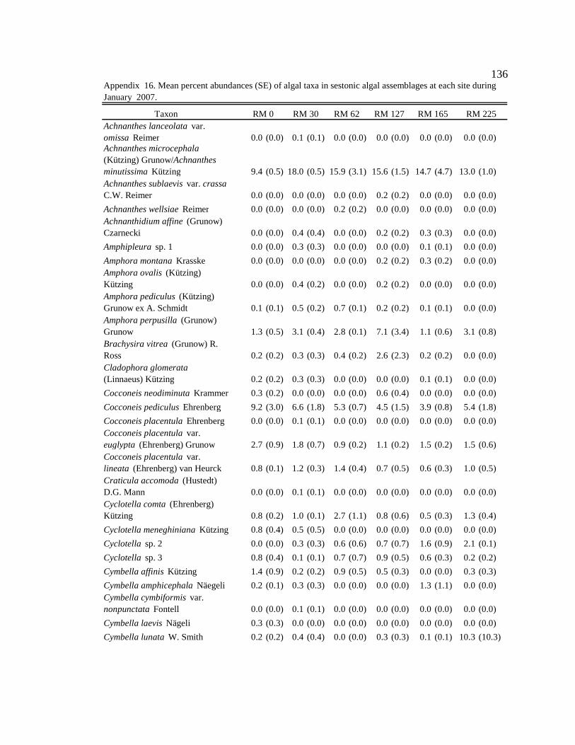
136
TaxonAchnanthes lanceolata var. omissa Reimer 0.0 (0.0) 0.1 (0.1) 0.0 (0.0) 0.0 (0.0) 0.0 (0.0) 0.0 (0.0)Achnanthes microcephala (Kützing) Grunow/Achnanthes minutissima Kützing 9.4 (0.5) 18.0 (0.5) 15.9 (3.1) 15.6 (1.5) 14.7 (4.7) 13.0 (1.0)Achnanthes sublaevis var. crassa C.W. Reimer 0.0 (0.0) 0.0 (0.0) 0.0 (0.0) 0.2 (0.2) 0.0 (0.0) 0.0 (0.0)
Achnanthes wellsiae Reimer 0.0 (0.0) 0.0 (0.0) 0.2 (0.2) 0.0 (0.0) 0.0 (0.0) 0.0 (0.0)Achnanthidium affine (Grunow) Czarnecki 0.0 (0.0) 0.4 (0.4) 0.0 (0.0) 0.2 (0.2) 0.3 (0.3) 0.0 (0.0)
Amphipleura sp. 1 0.0 (0.0) 0.3 (0.3) 0.0 (0.0) 0.0 (0.0) 0.1 (0.1) 0.0 (0.0)
Amphora montana Krasske 0.0 (0.0) 0.0 (0.0) 0.0 (0.0) 0.2 (0.2) 0.3 (0.2) 0.0 (0.0)Amphora ovalis (Kützing) Kützing 0.0 (0.0) 0.4 (0.2) 0.0 (0.0) 0.2 (0.2) 0.0 (0.0) 0.0(0.0)Amphora pediculus (Kützing) Grunow ex A. Schmidt 0.1 (0.1) 0.5 (0.2) 0.7 (0.1) 0.2 (0.2) 0.1 (0.1) 0.0 (0.0)Amphora perpusilla (Grunow) Grunow 1.3 (0.5) 3.1 (0.4) 2.8 (0.1) 7.1 (3.4) 1.1 (0.6) 3.1 (0.8)Brachysira vitrea (Grunow) R. Ross 0.2 (0.2) 0.3 (0.3) 0.4 (0.2) 2.6 (2.3) 0.2 (0.2) 0.0 (0.0)Cladophora glomerata (Linnaeus) Kützing 0.2 (0.2) 0.3 (0.3) 0.0 (0.0) 0.0 (0.0) 0.1 (0.1) 0.0 (0.0)
Cocconeis neodiminuta Krammer 0.3 (0.2) 0.0 (0.0) 0.0 (0.0) 0.6 (0.4) 0.0 (0.0) 0.0 (0.0)
Cocconeis pediculus Ehrenberg 9.2 (3.0) 6.6 (1.8) 5.3 (0.7) 4.5 (1.5) 3.9 (0.8) 5.4 (1.8)
Cocconeis placentula Ehrenberg 0.0 (0.0) 0.1 (0.1) 0.0 (0.0) 0.0 (0.0) 0.0 (0.0) 0.0 (0.0)Cocconeis placentula var. euglypta (Ehrenberg) Grunow 2.7 (0.9) 1.8 (0.7) 0.9 (0.2) 1.1 (0.2) 1.5 (0.2) 1.5 (0.6)Cocconeis placentula var. lineata (Ehrenberg) van Heurck 0.8 (0.1) 1.2 (0.3) 1.4 (0.4) 0.7 (0.5) 0.6 (0.3) 1.0 (0.5)Craticula accomoda (Hustedt) D.G. Mann 0.0 (0.0) 0.1 (0.1) 0.0 (0.0) 0.0 (0.0) 0.0 (0.0) 0.0 (0.0)Cyclotella comta (Ehrenberg) Kützing 0.8 (0.2) 1.0 (0.1) 2.7 (1.1) 0.8 (0.6) 0.5 (0.3) 1.3 (0.4)
Cyclotella meneghiniana Kützing 0.8 (0.4) 0.5 (0.5) 0.0 (0.0) 0.0 (0.0) 0.0 (0.0) 0.0 (0.0)
Cyclotella sp. 2 0.0 (0.0) 0.3 (0.3) 0.6 (0.6) 0.7 (0.7) 1.6 (0.9) 2.1 (0.1)
Cyclotella sp. 3 0.8 (0.4) 0.1 (0.1) 0.7 (0.7) 0.9 (0.5) 0.6 (0.3) 0.2 (0.2)
Cymbella affinis Kützing 1.4 (0.9) 0.2 (0.2) 0.9 (0.5) 0.5 (0.3) 0.0 (0.0) 0.3 (0.3)
Cymbella amphicephala Näegeli 0.2 (0.1) 0.3 (0.3) 0.0 (0.0) 0.0 (0.0) 1.3 (1.1) 0.0 (0.0)Cymbella cymbiformis var. nonpunctata Fontell 0.0 (0.0) 0.1 (0.1) 0.0 (0.0) 0.0 (0.0) 0.0 (0.0) 0.0 (0.0)
Cymbella laevis Nägeli 0.3 (0.3) 0.0 (0.0) 0.0 (0.0) 0.0 (0.0) 0.0 (0.0) 0.0 (0.0)
Cymbella lunata W. Smith 0.2 (0.2) 0.4 (0.4) 0.0 (0.0) 0.3 (0.3) 0.1 (0.1) 10.3 (10.3)
Appendix 16. Mean percent abundances (SE) of algal taxa in sestonic algal assemblages at each site during January 2007.
RM 0 RM 30 RM 62 RM 127 RM 165 RM 225
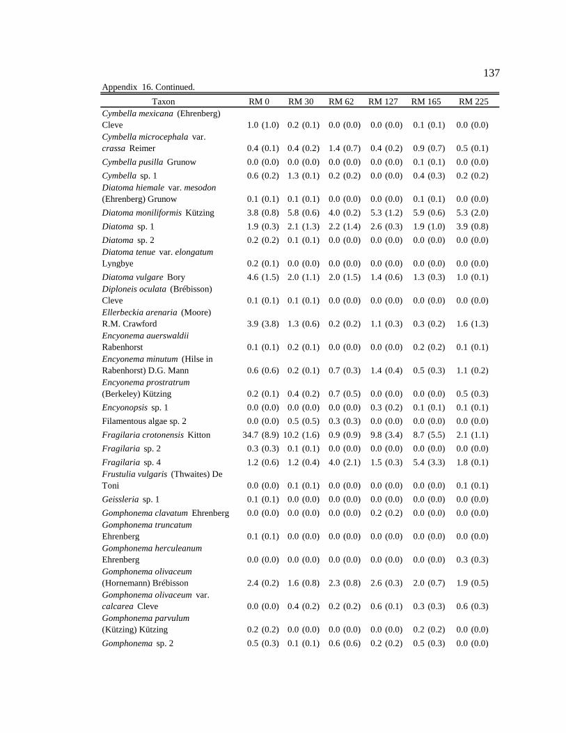
137
TaxonCymbella mexicana (Ehrenberg) Cleve 1.0 (1.0) 0.2 (0.1) 0.0 (0.0) 0.0 (0.0) 0.1 (0.1) 0.0 (0.0)Cymbella microcephala var. crassa Reimer 0.4 (0.1) 0.4 (0.2) 1.4 (0.7) 0.4 (0.2) 0.9 (0.7) 0.5 (0.1)
Cymbella pusilla Grunow 0.0 (0.0) 0.0 (0.0) 0.0 (0.0) 0.0 (0.0) 0.1 (0.1) 0.0 (0.0)
Cymbella sp. 1 0.6 (0.2) 1.3 (0.1) 0.2 (0.2) 0.0 (0.0) 0.4 (0.3) 0.2 (0.2)Diatoma hiemale var. mesodon (Ehrenberg) Grunow 0.1 (0.1) 0.1 (0.1) 0.0 (0.0) 0.0 (0.0) 0.1 (0.1) 0.0 (0.0)
Diatoma moniliformis Kützing 3.8 (0.8) 5.8 (0.6) 4.0 (0.2) 5.3 (1.2) 5.9 (0.6) 5.3 (2.0)
Diatoma sp. 1 1.9 (0.3) 2.1 (1.3) 2.2 (1.4) 2.6 (0.3) 1.9 (1.0) 3.9 (0.8)
Diatoma sp. 2 0.2 (0.2) 0.1 (0.1) 0.0 (0.0) 0.0 (0.0) 0.0 (0.0) 0.0 (0.0)Diatoma tenue var. elongatum Lyngbye 0.2 (0.1) 0.0 (0.0) 0.0 (0.0) 0.0 (0.0) 0.0 (0.0) 0.0 (0.0)
Diatoma vulgare Bory 4.6 (1.5) 2.0 (1.1) 2.0 (1.5) 1.4 (0.6) 1.3 (0.3) 1.0 (0.1)Diploneis oculata (Brébisson) Cleve 0.1 (0.1) 0.1 (0.1) 0.0 (0.0) 0.0 (0.0) 0.0 (0.0) 0.0 (0.0)Ellerbeckia arenaria (Moore) R.M. Crawford 3.9 (3.8) 1.3 (0.6) 0.2 (0.2) 1.1 (0.3) 0.3 (0.2) 1.6 (1.3)Encyonema auerswaldii Rabenhorst 0.1 (0.1) 0.2 (0.1) 0.0 (0.0) 0.0 (0.0) 0.2 (0.2) 0.1 (0.1)Encyonema minutum (Hilse in Rabenhorst) D.G. Mann 0.6 (0.6) 0.2 (0.1) 0.7 (0.3) 1.4 (0.4) 0.5 (0.3) 1.1 (0.2)Encyonema prostratrum (Berkeley) Kützing 0.2 (0.1) 0.4 (0.2) 0.7 (0.5) 0.0 (0.0) 0.0 (0.0) 0.5 (0.3)
Encyonopsis sp. 1 0.0 (0.0) 0.0 (0.0) 0.0 (0.0) 0.3 (0.2) 0.1 (0.1) 0.1 (0.1)
Filamentous algae sp. 2 0.0 (0.0) 0.5 (0.5) 0.3 (0.3) 0.0 (0.0) 0.0 (0.0) 0.0 (0.0)
Fragilaria crotonensis Kitton 34.7 (8.9) 10.2 (1.6) 0.9 (0.9) 9.8 (3.4) 8.7 (5.5) 2.1 (1.1)
Fragilaria sp. 2 0.3 (0.3) 0.1 (0.1) 0.0 (0.0) 0.0 (0.0) 0.0 (0.0) 0.0 (0.0)
Fragilaria sp. 4 1.2 (0.6) 1.2 (0.4) 4.0 (2.1) 1.5 (0.3) 5.4 (3.3) 1.8 (0.1)Frustulia vulgaris (Thwaites) De Toni 0.0 (0.0) 0.1 (0.1) 0.0 (0.0) 0.0 (0.0) 0.0 (0.0) 0.1 (0.1)
Geissleria sp. 1 0.1 (0.1) 0.0 (0.0) 0.0 (0.0) 0.0 (0.0) 0.0 (0.0) 0.0 (0.0)
Gomphonema clavatum Ehrenberg 0.0 (0.0) 0.0 (0.0) 0.0 (0.0) 0.2 (0.2) 0.0 (0.0) 0.0 (0.0)Gomphonema truncatum Ehrenberg 0.1 (0.1) 0.0 (0.0) 0.0 (0.0) 0.0 (0.0) 0.0 (0.0) 0.0 (0.0)Gomphonema herculeanum Ehrenberg 0.0 (0.0) 0.0 (0.0) 0.0 (0.0) 0.0 (0.0) 0.0 (0.0) 0.3 (0.3)Gomphonema olivaceum (Hornemann) Brébisson 2.4 (0.2) 1.6 (0.8) 2.3 (0.8) 2.6 (0.3) 2.0 (0.7) 1.9 (0.5)Gomphonema olivaceum var. calcarea Cleve 0.0 (0.0) 0.4 (0.2) 0.2 (0.2) 0.6 (0.1) 0.3 (0.3) 0.6 (0.3)Gomphonema parvulum (Kützing) Kützing 0.2 (0.2) 0.0 (0.0) 0.0 (0.0) 0.0 (0.0) 0.2 (0.2) 0.0 (0.0)
Gomphonema sp. 2 0.5 (0.3) 0.1 (0.1) 0.6 (0.6) 0.2 (0.2) 0.5 (0.3) 0.0 (0.0)
Appendix 16. Continued.
RM 0 RM 30 RM 62 RM 127 RM 165 RM 225
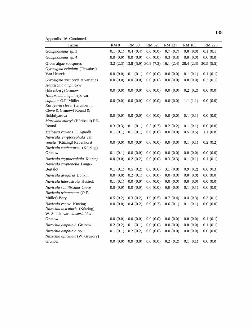
138
Taxon
Gomphonema sp. 3 0.1 (0.1) 0.4 (0.4) 0.0 (0.0) 0.7 (0.7) 0.0 (0.0) 0.1 (0.1)
Gomphonema sp. 4 0.0 (0.0) 0.0 (0.0) 0.0 (0.0) 0.3 (0.3) 0.0 (0.0) 0.0 (0.0)
Green algae zoospores 3.2 (2.3) 13.8 (5.9) 30.9 (7.3) 16.1 (2.4) 28.4 (2.3) 20.5 (5.5)Gyrosigma eximium (Thwaites) Van Heurck 0.0 (0.0) 0.1 (0.1) 0.0 (0.0) 0.0 (0.0) 0.1 (0.1)0.1 (0.1)
Gyrosigma spencerii et varieties 0.0 (0.0) 0.0 (0.0) 0.0 (0.0) 0.0 (0.0) 0.0 (0.0) 0.2 (0.1)Hantzschia amphioxys (Ehrenberg) Grunow 0.0 (0.0) 0.0 (0.0) 0.0 (0.0) 0.0 (0.0) 0.2 (0.2) 0.0 (0.0)Hantzschia amphioxys var. capitata O.F. Müller 0.0 (0.0) 0.0 (0.0) 0.0 (0.0) 0.0 (0.0) 1.1 (1.1) 0.0 (0.0)Karayevia clevei (Grunow in Cleve & Grunow) Round & Bukhtiyarova 0.0 (0.0) 0.0 (0.0) 0.0 (0.0) 0.0 (0.0) 0.1 (0.1) 0.0 (0.0)Martyana martyi (Héribaud) F.E. Round 0.3 (0.3) 0.1 (0.1) 0.3 (0.3) 0.2 (0.2) 0.1 (0.1) 0.0 (0.0)
Melosira varians C. Agardh 0.1 (0.1) 0.1 (0.1) 0.6 (0.6) 0.0 (0.0) 0.5 (0.5) 1.1 (0.8)Navicula cryptocephala var. veneta (Kützing) Rabenhorst 0.0 (0.0) 0.0 (0.0) 0.0 (0.0) 0.0 (0.0) 0.1 (0.1) 0.2 (0.2)Navicula confervacea (Kützing) Grunow 0.1 (0.1) 0.0 (0.0) 0.0 (0.0) 0.0 (0.0) 0.0 (0.0) 0.0 (0.0)
Navicula cryptocephala Kützing 0.0 (0.0) 0.2 (0.2) 0.0 (0.0) 0.3 (0.3) 0.1 (0.1) 0.1 (0.1)Navicula cryptonella Lange-Bertalot 0.1 (0.1) 0.5 (0.2) 0.6 (0.6) 3.1 (0.8) 0.9 (0.2) 0.6 (0.3)
Navicula gregaria Donkin 0.0 (0.0) 0.2 (0.1) 0.0 (0.0) 0.0 (0.0) 0.0 (0.0) 0.0 (0.0)
Navicula laterostrata Hustedt 0.1 (0.1) 0.0 (0.0) 0.0 (0.0) 0.0 (0.0) 0.0 (0.0) 0.0 (0.0)
Navicula subtilissima Cleve 0.0 (0.0) 0.0 (0.0) 0.0 (0.0) 0.0 (0.0) 0.1 (0.1) 0.0 (0.0)Navicula tripunctata (O.F. Müller) Bory 0.5 (0.2) 0.3 (0.2) 1.0 (0.5) 0.7 (0.4) 0.4 (0.3) 0.3 (0.1)
Navicula veneta Kützing 0.0 (0.0) 0.4 (0.2) 0.9 (0.2) 0.6 (0.1) 0.1 (0.1) 0.0 (0.0)Nitzschia acicularis (Kützing) W. Smith var. closterioides Grunow 0.0 (0.0) 0.0 (0.0) 0.0 (0.0) 0.0 (0.0) 0.0 (0.0) 0.1 (0.1)
Nitzschia amphibia Grunow 0.2 (0.2) 0.1 (0.1) 0.0 (0.0) 0.0 (0.0) 0.0 (0.0) 0.1 (0.1)
Nitzschia amphibia sp. 1 0.1 (0.1) 0.2 (0.2) 0.0 (0.0) 0.0 (0.0) 0.0 (0.0) 0.0 (0.0)Nitzschia apiculata(W. Gregory) Grunow 0.0 (0.0) 0.0 (0.0) 0.0 (0.0) 0.2 (0.2) 0.1 (0.1) 0.0 (0.0)
Appendix 16. Continued.
RM 0 RM 30 RM 62 RM 127 RM 165 RM 225
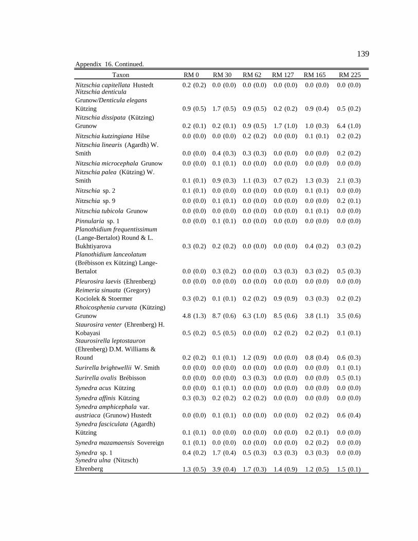
139
Taxon
Nitzschia capitellata Hustedt 0.2 (0.2) 0.0 (0.0) 0.0 (0.0) 0.0 (0.0) 0.0 (0.0) 0.0 (0.0)Nitzschia denticula Grunow/Denticula elegans Kützing 0.9 (0.5) 1.7 (0.5) 0.9 (0.5) 0.2 (0.2) 0.9 (0.4) 0.5 (0.2)Nitzschia dissipata (Kützing) Grunow 0.2 (0.1) 0.2 (0.1) 0.9 (0.5) 1.7 (1.0) 1.0 (0.3) 6.4 (1.0)
Nitzschia kutzingiana Hilse 0.0 (0.0) 0.0 (0.0) 0.2 (0.2) 0.0 (0.0) 0.1 (0.1) 0.2 (0.2)Nitzschia linearis (Agardh) W. Smith 0.0 (0.0) 0.4 (0.3) 0.3 (0.3) 0.0 (0.0) 0.0 (0.0) 0.2 (0.2)
Nitzschia microcephala Grunow 0.0 (0.0) 0.1 (0.1) 0.0 (0.0) 0.0 (0.0) 0.0 (0.0) 0.0 (0.0)Nitzschia palea (Kützing) W. Smith 0.1 (0.1) 0.9 (0.3) 1.1 (0.3) 0.7 (0.2) 1.3 (0.3) 2.1 (0.3)
Nitzschia sp. 2 0.1 (0.1) 0.0 (0.0) 0.0 (0.0) 0.0 (0.0) 0.1 (0.1) 0.0 (0.0)
Nitzschia sp. 9 0.0 (0.0) 0.1 (0.1) 0.0 (0.0) 0.0 (0.0) 0.0 (0.0) 0.2 (0.1)
Nitzschia tubicola Grunow 0.0 (0.0) 0.0 (0.0) 0.0 (0.0) 0.0 (0.0) 0.1 (0.1) 0.0 (0.0)
Pinnularia sp. 1 0.0 (0.0) 0.1 (0.1) 0.0 (0.0) 0.0 (0.0) 0.0 (0.0) 0.0 (0.0)Planothidium frequentissimum (Lange-Bertalot) Round & L. Bukhtiyarova 0.3 (0.2) 0.2 (0.2) 0.0 (0.0) 0.0 (0.0) 0.4 (0.2) 0.3 (0.2)Planothidium lanceolatum (Brébisson ex Kützing) Lange-Bertalot 0.0 (0.0) 0.3 (0.2) 0.0 (0.0) 0.3 (0.3) 0.3 (0.2) 0.5 (0.3)
Pleurosira laevis (Ehrenberg) 0.0 (0.0) 0.0 (0.0) 0.0 (0.0) 0.0 (0.0) 0.0 (0.0) 0.0 (0.0)Reimeria sinuata (Gregory) Kociolek & Stoermer 0.3 (0.2) 0.1 (0.1) 0.2 (0.2) 0.9 (0.9) 0.3 (0.3) 0.2 (0.2)Rhoicosphenia curvata (Kützing) Grunow 4.8 (1.3) 8.7 (0.6) 6.3 (1.0) 8.5 (0.6) 3.8 (1.1) 3.5 (0.6)Staurosira venter (Ehrenberg) H. Kobayasi 0.5 (0.2) 0.5 (0.5) 0.0 (0.0) 0.2 (0.2) 0.2 (0.2) 0.1 (0.1)Staurosirella leptostauron (Ehrenberg) D.M. Williams & Round 0.2 (0.2) 0.1 (0.1) 1.2 (0.9) 0.0 (0.0) 0.8 (0.4) 0.6 (0.3)
Surirella brightwellii W. Smith 0.0 (0.0) 0.0 (0.0) 0.0 (0.0) 0.0 (0.0) 0.0 (0.0) 0.1 (0.1)
Surirella ovalis Brébisson 0.0 (0.0) 0.0 (0.0) 0.3 (0.3) 0.0 (0.0) 0.0 (0.0) 0.5 (0.1)
Synedra acus Kützing 0.0 (0.0) 0.1 (0.1) 0.0 (0.0) 0.0 (0.0) 0.0 (0.0) 0.0 (0.0)
Synedra affinis Kützing 0.3 (0.3) 0.2 (0.2) 0.2 (0.2) 0.0 (0.0) 0.0 (0.0) 0.0 (0.0)Synedra amphicephala var. austriaca (Grunow) Hustedt 0.0 (0.0) 0.1 (0.1) 0.0 (0.0) 0.0 (0.0) 0.2(0.2) 0.6 (0.4)Synedra fasciculata (Agardh) Kützing 0.1 (0.1) 0.0 (0.0) 0.0 (0.0) 0.0 (0.0) 0.2 (0.1) 0.0 (0.0)
Synedra mazamaensis Sovereign 0.1 (0.1) 0.0 (0.0) 0.0 (0.0) 0.0 (0.0) 0.2 (0.2) 0.0 (0.0)
Synedra sp. 1 0.4 (0.2) 1.7 (0.4) 0.5 (0.3) 0.3 (0.3) 0.3 (0.3) 0.0 (0.0)Synedra ulna (Nitzsch) Ehrenberg 1.3 (0.5) 3.9 (0.4) 1.7 (0.3) 1.4 (0.9) 1.2 (0.5) 1.5 (0.1)
Appendix 16. Continued.
RM 0 RM 30 RM 62 RM 127 RM 165 RM 225
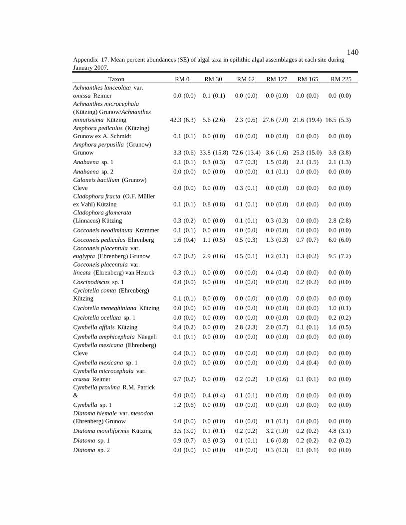
140
TaxonAchnanthes lanceolata var. omissa Reimer 0.0 (0.0) 0.1 (0.1) 0.0 (0.0) 0.0 (0.0) 0.0 (0.0) 0.0 (0.0)Achnanthes microcephala (Kützing) Grunow/Achnanthes minutissima Kützing 42.3 (6.3) 5.6 (2.6) 2.3 (0.6) 27.6 (7.0) 21.6 (19.4)16.5 (5.3)Amphora pediculus (Kützing) Grunow ex A. Schmidt 0.1 (0.1) 0.0 (0.0) 0.0 (0.0) 0.0 (0.0) 0.0 (0.0) 0.0 (0.0)Amphora perpusilla (Grunow) Grunow 3.3 (0.6) 33.8 (15.8) 72.6 (13.4) 3.6 (1.6) 25.3 (15.0) 3.8 (3.8)
Anabaena sp. 1 0.1 (0.1) 0.3 (0.3) 0.7 (0.3) 1.5 (0.8) 2.1 (1.5) 2.1 (1.3)
Anabaena sp. 2 0.0 (0.0) 0.0 (0.0) 0.0 (0.0) 0.1 (0.1) 0.0 (0.0) 0.0 (0.0)Caloneis bacillum (Grunow) Cleve 0.0 (0.0) 0.0 (0.0) 0.3 (0.1) 0.0 (0.0) 0.0 (0.0) 0.0 (0.0)Cladophora fracta (O.F. Müller ex Vahl) Kützing 0.1 (0.1) 0.8 (0.8) 0.1 (0.1) 0.0 (0.0) 0.0 (0.0) 0.0 (0.0)Cladophora glomerata (Linnaeus) Kützing 0.3 (0.2) 0.0 (0.0) 0.1 (0.1) 0.3 (0.3) 0.0 (0.0) 2.8 (2.8)
Cocconeis neodiminuta Krammer 0.1 (0.1) 0.0 (0.0) 0.0 (0.0) 0.0 (0.0) 0.0 (0.0) 0.0 (0.0)
Cocconeis pediculus Ehrenberg 1.6 (0.4) 1.1 (0.5) 0.5 (0.3) 1.3 (0.3) 0.7 (0.7) 6.0 (6.0)Cocconeis placentula var. euglypta (Ehrenberg) Grunow 0.7 (0.2) 2.9 (0.6) 0.5 (0.1) 0.2 (0.1)0.3 (0.2) 9.5 (7.2)Cocconeis placentula var. lineata (Ehrenberg) van Heurck 0.3 (0.1) 0.0 (0.0) 0.0 (0.0) 0.4 (0.4) 0.0 (0.0) 0.0 (0.0)
Coscinodiscus sp. 1 0.0 (0.0) 0.0 (0.0) 0.0 (0.0) 0.0 (0.0) 0.2 (0.2) 0.0 (0.0)Cyclotella comta (Ehrenberg) Kützing 0.1 (0.1) 0.0 (0.0) 0.0 (0.0) 0.0 (0.0) 0.0 (0.0) 0.0 (0.0)
Cyclotella meneghiniana Kützing 0.0 (0.0) 0.0 (0.0) 0.0 (0.0) 0.0 (0.0) 0.0 (0.0) 1.0 (0.1)
Cyclotella ocellata sp. 1 0.0 (0.0) 0.0 (0.0) 0.0 (0.0) 0.0 (0.0) 0.0 (0.0) 0.2 (0.2)
Cymbella affinis Kützing 0.4 (0.2) 0.0 (0.0) 2.8 (2.3) 2.0 (0.7) 0.1 (0.1) 1.6 (0.5)
Cymbella amphicephala Näegeli 0.1 (0.1) 0.0 (0.0) 0.0 (0.0) 0.0 (0.0) 0.0 (0.0) 0.0 (0.0)Cymbella mexicana (Ehrenberg) Cleve 0.4 (0.1) 0.0 (0.0) 0.0 (0.0) 0.0 (0.0) 0.0 (0.0) 0.0 (0.0)
Cymbella mexicana sp. 1 0.0 (0.0) 0.0 (0.0) 0.0 (0.0) 0.0 (0.0) 0.4 (0.4) 0.0 (0.0)Cymbella microcephala var. crassa Reimer 0.7 (0.2) 0.0 (0.0) 0.2 (0.2) 1.0 (0.6) 0.1 (0.1) 0.0 (0.0)Cymbella proxima R.M. Patrick & 0.0 (0.0) 0.4 (0.4) 0.1 (0.1) 0.0 (0.0) 0.0 (0.0) 0.0 (0.0)
Cymbella sp. 1 1.2 (0.6) 0.0 (0.0) 0.0 (0.0) 0.0 (0.0) 0.0 (0.0) 0.0 (0.0)Diatoma hiemale var. mesodon (Ehrenberg) Grunow 0.0 (0.0) 0.0 (0.0) 0.0 (0.0) 0.1 (0.1) 0.0 (0.0) 0.0 (0.0)
Diatoma moniliformis Kützing 3.5 (3.0) 0.1 (0.1) 0.2 (0.2) 3.2 (1.0) 0.2 (0.2) 4.8 (3.1)
Diatoma sp. 1 0.9 (0.7) 0.3 (0.3) 0.1 (0.1) 1.6 (0.8) 0.2 (0.2) 0.2 (0.2)
Diatoma sp. 2 0.0 (0.0) 0.0 (0.0) 0.0 (0.0) 0.3 (0.3) 0.1 (0.1) 0.0 (0.0)
Appendix 17. Mean percent abundances (SE) of algal taxa in epilithic algal assemblages at each site during January 2007.
RM 0 RM 30 RM 62 RM 127 RM 165 RM 225
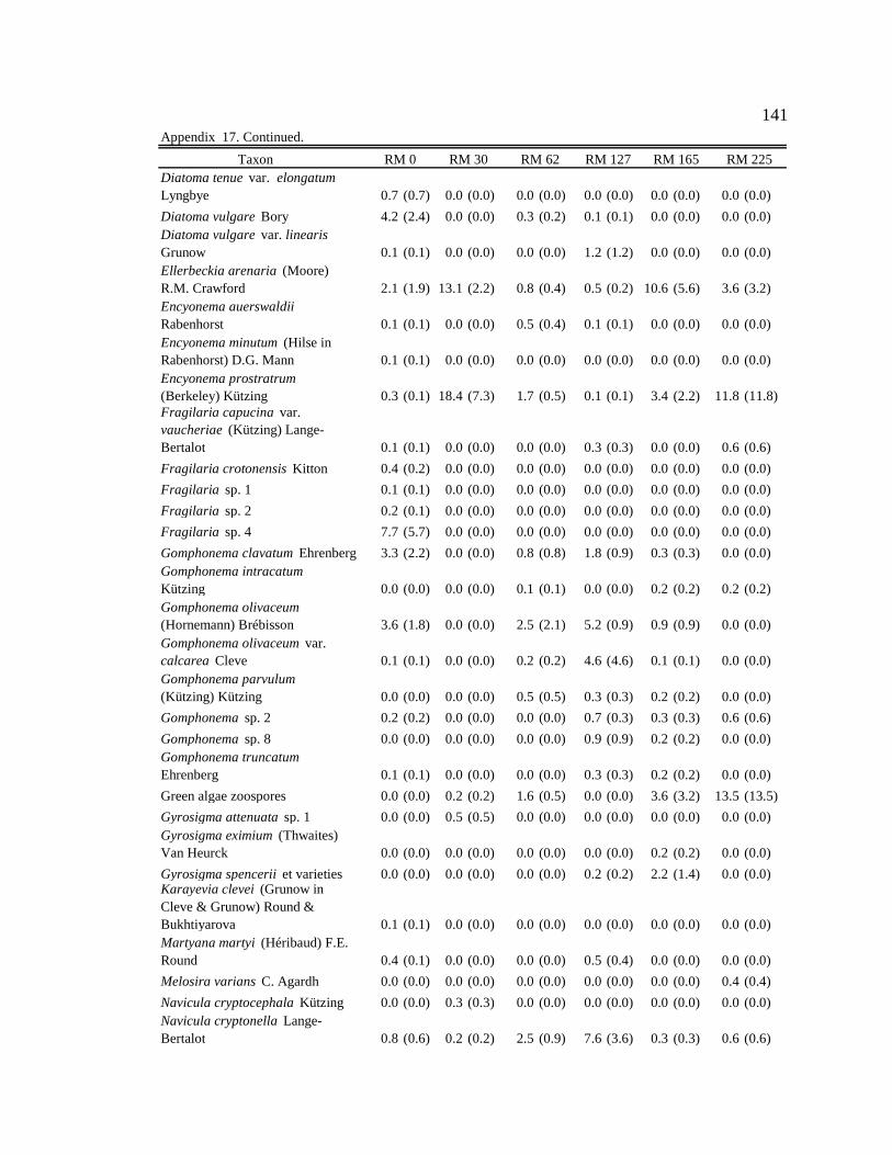
141
TaxonDiatoma tenue var. elongatum Lyngbye 0.7 (0.7) 0.0 (0.0) 0.0 (0.0) 0.0 (0.0) 0.0 (0.0) 0.0 (0.0)
Diatoma vulgare Bory 4.2 (2.4) 0.0 (0.0) 0.3 (0.2) 0.1 (0.1) 0.0 (0.0) 0.0 (0.0)Diatoma vulgare var. linearis Grunow 0.1 (0.1) 0.0 (0.0) 0.0 (0.0) 1.2 (1.2) 0.0 (0.0) 0.0 (0.0)Ellerbeckia arenaria (Moore) R.M. Crawford 2.1 (1.9) 13.1 (2.2) 0.8 (0.4) 0.5 (0.2) 10.6 (5.6) 3.6 (3.2)Encyonema auerswaldii Rabenhorst 0.1 (0.1) 0.0 (0.0) 0.5 (0.4) 0.1 (0.1) 0.0 (0.0) 0.0 (0.0)Encyonema minutum (Hilse in Rabenhorst) D.G. Mann 0.1 (0.1) 0.0 (0.0) 0.0 (0.0) 0.0(0.0) 0.0 (0.0) 0.0 (0.0)Encyonema prostratrum (Berkeley) Kützing 0.3 (0.1) 18.4 (7.3) 1.7 (0.5) 0.1 (0.1) 3.4 (2.2) 11.8 (11.8)Fragilaria capucina var. vaucheriae (Kützing) Lange-Bertalot 0.1 (0.1) 0.0 (0.0) 0.0 (0.0) 0.3 (0.3) 0.0 (0.0) 0.6 (0.6)
Fragilaria crotonensis Kitton 0.4 (0.2) 0.0 (0.0) 0.0 (0.0) 0.0 (0.0) 0.0 (0.0) 0.0 (0.0)
Fragilaria sp. 1 0.1 (0.1) 0.0 (0.0) 0.0 (0.0) 0.0 (0.0) 0.0 (0.0) 0.0 (0.0)
Fragilaria sp. 2 0.2 (0.1) 0.0 (0.0) 0.0 (0.0) 0.0 (0.0) 0.0 (0.0) 0.0 (0.0)
Fragilaria sp. 4 7.7 (5.7) 0.0 (0.0) 0.0 (0.0) 0.0 (0.0) 0.0 (0.0) 0.0 (0.0)
Gomphonema clavatum Ehrenberg 3.3 (2.2) 0.0 (0.0) 0.8 (0.8) 1.8 (0.9) 0.3 (0.3) 0.0 (0.0)Gomphonema intracatum Kützing 0.0 (0.0) 0.0 (0.0) 0.1 (0.1) 0.0 (0.0) 0.2 (0.2) 0.2 (0.2)Gomphonema olivaceum (Hornemann) Brébisson 3.6 (1.8) 0.0 (0.0) 2.5 (2.1) 5.2 (0.9) 0.9 (0.9) 0.0 (0.0)Gomphonema olivaceum var. calcarea Cleve 0.1 (0.1) 0.0 (0.0) 0.2 (0.2) 4.6 (4.6) 0.1 (0.1) 0.0 (0.0)Gomphonema parvulum (Kützing) Kützing 0.0 (0.0) 0.0 (0.0) 0.5 (0.5) 0.3 (0.3) 0.2 (0.2) 0.0 (0.0)
Gomphonema sp. 2 0.2 (0.2) 0.0 (0.0) 0.0 (0.0) 0.7 (0.3) 0.3 (0.3) 0.6 (0.6)
Gomphonema sp. 8 0.0 (0.0) 0.0 (0.0) 0.0 (0.0) 0.9 (0.9) 0.2 (0.2) 0.0 (0.0)Gomphonema truncatum Ehrenberg 0.1 (0.1) 0.0 (0.0) 0.0 (0.0) 0.3 (0.3) 0.2 (0.2) 0.0 (0.0)
Green algae zoospores 0.0 (0.0) 0.2 (0.2) 1.6 (0.5) 0.0 (0.0) 3.6 (3.2) 13.5 (13.5)
Gyrosigma attenuata sp. 1 0.0 (0.0) 0.5 (0.5) 0.0 (0.0) 0.0 (0.0) 0.0 (0.0) 0.0 (0.0)Gyrosigma eximium (Thwaites) Van Heurck 0.0 (0.0) 0.0 (0.0) 0.0 (0.0) 0.0 (0.0) 0.2 (0.2)0.0 (0.0)
Gyrosigma spencerii et varieties 0.0 (0.0) 0.0 (0.0) 0.0 (0.0) 0.2 (0.2) 2.2 (1.4) 0.0 (0.0)Karayevia clevei (Grunow in Cleve & Grunow) Round & Bukhtiyarova 0.1 (0.1) 0.0 (0.0) 0.0 (0.0) 0.0 (0.0) 0.0 (0.0) 0.0 (0.0)Martyana martyi (Héribaud) F.E. Round 0.4 (0.1) 0.0 (0.0) 0.0 (0.0) 0.5 (0.4) 0.0 (0.0) 0.0 (0.0)
Melosira varians C. Agardh 0.0 (0.0) 0.0 (0.0) 0.0 (0.0) 0.0 (0.0) 0.0 (0.0) 0.4 (0.4)
Navicula cryptocephala Kützing 0.0 (0.0) 0.3 (0.3) 0.0 (0.0) 0.0 (0.0) 0.0 (0.0) 0.0 (0.0)Navicula cryptonella Lange-Bertalot 0.8 (0.6) 0.2 (0.2) 2.5 (0.9) 7.6 (3.6) 0.3 (0.3) 0.6 (0.6)
Appendix 17. Continued.
RM 0 RM 30 RM 62 RM 127 RM 165 RM 225
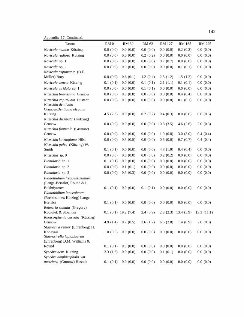
142
Taxon
Navicula mutica Kützing 0.0 (0.0) 0.0 (0.0) 0.0 (0.0) 0.0 (0.0) 0.2 (0.2) 0.0 (0.0)
Navicula radiosa Kützing 0.0 (0.0) 0.0 (0.0) 0.2 (0.2) 0.0 (0.0) 0.0 (0.0) 0.0 (0.0)
Navicula sp. 1 0.0 (0.0) 0.0 (0.0) 0.0 (0.0) 0.7 (0.7) 0.0 (0.0) 0.0 (0.0)
Navicula sp. 2 0.0 (0.0) 0.0 (0.0) 0.0 (0.0) 0.0 (0.0) 0.1 (0.1) 0.0 (0.0)Navicula tripunctata (O.F. Müller) Bory 0.0 (0.0) 0.6 (0.1) 1.2 (0.4) 2.5 (1.2) 1.5 (1.2) 0.0 (0.0)
Navicula veneta Kützing 0.1 (0.1) 0.0 (0.0) 0.1 (0.1) 2.1 (1.1) 0.1 (0.1) 0.0 (0.0)
Navicula viridula sp. 1 0.0 (0.0) 0.0 (0.0) 0.1 (0.1) 0.0 (0.0) 0.0 (0.0) 0.0 (0.0)
Nitzschia brevissima Grunow 0.0 (0.0) 0.0 (0.0) 0.0 (0.0) 0.0 (0.0) 0.4 (0.4) 0.0 (0.0)
Nitzschia capitellata Hustedt 0.0 (0.0) 0.0 (0.0) 0.0 (0.0) 0.0 (0.0) 0.1 (0.1) 0.0 (0.0)Nitzschia denticula Grunow/Denticula elegans Kützing 4.5 (2.3) 0.0 (0.0) 0.2 (0.2) 0.4 (0.3) 0.0 (0.0) 0.6 (0.6)Nitzschia dissipata (Kützing) Grunow 0.0 (0.0) 0.0 (0.0) 0.0 (0.0) 10.8 (3.5) 4.6 (2.6) 2.0 (0.3)Nitzschia fonticola (Grunow) Grunow 0.0 (0.0) 0.0 (0.0) 0.0 (0.0) 1.0 (0.8) 3.0 (3.0) 0.4 (0.4)
Nitzschia kutzingiana Hilse 0.0 (0.0) 0.5 (0.5) 0.0 (0.0) 0.5 (0.0) 0.7 (0.7) 0.4 (0.4)Nitzschia palea (Kützing) W. Smith 0.1 (0.1) 0.0 (0.0) 0.0 (0.0) 4.8 (1.9) 0.4 (0.4) 0.0 (0.0)
Nitzschia sp. 9 0.0 (0.0) 0.0 (0.0) 0.0 (0.0) 0.2 (0.2) 0.0 (0.0) 0.0 (0.0)
Pinnularia sp. 1 0.1 (0.1) 0.0 (0.0) 0.0 (0.0) 0.0 (0.0) 0.0 (0.0) 0.0 (0.0)
Pinnularia sp. 2 0.0 (0.0) 0.1 (0.1) 0.0 (0.0) 0.0 (0.0) 0.0 (0.0) 0.0 (0.0)
Pinnularia sp. 3 0.0 (0.0) 0.3 (0.3) 0.0 (0.0) 0.0 (0.0) 0.0 (0.0) 0.0 (0.0)
Planothidium frequentissimum (Lange-Bertalot) Round & L. Bukhtiyarova 0.1 (0.1) 0.0 (0.0) 0.1 (0.1) 0.0 (0.0) 0.0 (0.0) 0.0 (0.0)Planothidium lanceolatum (Brébisson ex Kützing) Lange-Bertalot 0.1 (0.1) 0.0 (0.0) 0.0 (0.0) 0.0 (0.0) 0.0 (0.0) 0.0 (0.0)Reimeria sinuata (Gregory) Kociolek & Stoermer 0.1 (0.1) 19.2 (7.4) 2.4 (0.9) 2.3 (2.3) 13.4 (5.9) 13.3 (11.1)Rhoicosphenia curvata (Kützing) Grunow 4.9 (1.4) 0.7 (0.5) 3.6 (1.7) 6.6 (2.8) 1.4 (0.9) 2.0 (0.3)Staurosira venter (Ehrenberg) H. Kobayasi 1.0 (0.5) 0.0 (0.0) 0.0 (0.0) 0.0 (0.0) 0.0 (0.0) 0.0 (0.0)Staurosirella leptostauron (Ehrenberg) D.M. Williams & Round 0.1 (0.1) 0.0 (0.0) 0.0 (0.0) 0.0 (0.0) 0.0 (0.0) 0.0 (0.0)
Synedra acus Kützing 2.3 (1.3) 0.0 (0.0) 0.0 (0.0) 0.1 (0.1) 0.0 (0.0) 0.0 (0.0)Synedra amphicephala var. austriaca (Grunow) Hustedt 0.1 (0.1) 0.0 (0.0) 0.0 (0.0) 0.0 (0.0) 0.0 (0.0) 0.0 (0.0)
Appendix 17. Continued.
RM 0 RM 30 RM 62 RM 127 RM 165 RM 225
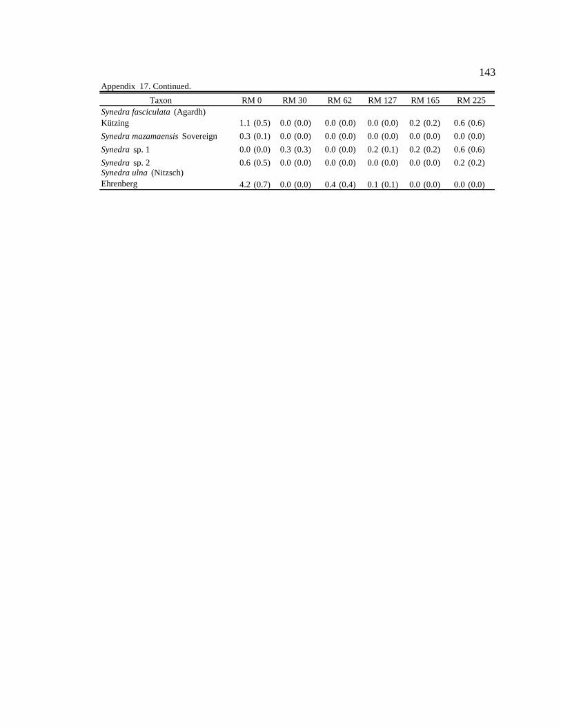
143
TaxonSynedra fasciculata (Agardh) Kützing 1.1 (0.5) 0.0 (0.0) 0.0 (0.0) 0.0 (0.0) 0.2 (0.2) 0.6 (0.6)
Synedra mazamaensis Sovereign 0.3 (0.1) 0.0 (0.0) 0.0 (0.0) 0.0 (0.0) 0.0 (0.0) 0.0 (0.0)
Synedra sp. 1 0.0 (0.0) 0.3 (0.3) 0.0 (0.0) 0.2 (0.1) 0.2 (0.2) 0.6 (0.6)
Synedra sp. 2 0.6 (0.5) 0.0 (0.0) 0.0 (0.0) 0.0 (0.0) 0.0 (0.0) 0.2 (0.2)Synedra ulna (Nitzsch) Ehrenberg 4.2 (0.7) 0.0 (0.0) 0.4 (0.4) 0.1 (0.1) 0.0 (0.0) 0.0 (0.0)
Appendix 17. Continued.
RM 0 RM 30 RM 62 RM 127 RM 165 RM 225
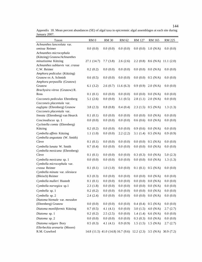
144
TaxonAchnanthes lanceolata var. omissa Reimer 0.0 (0.0) 0.0 (0.0) 0.0 (0.0) 0.0 (0.0) 1.0 (N/A) 0.0 (0.0)Achnanthes microcephala (Kützing) Grunow/Achnanthes minutissima Kützing 27.1 (14.7) 7.7 (3.8) 2.6 (2.6) 2.2 (0.8) 8.6 (N/A) 11.1 (2.0)Achnanthes sublaevis var. crassa C.W. Reimer 0.2 (0.2) 0.0 (0.0) 0.0 (0.0) 0.0 (0.0) 0.0 (N/A)0.0 (0.0)Amphora pediculus (Kützing) Grunow ex A. Schmidt 0.6 (0.5) 0.0 (0.0) 0.0 (0.0) 0.0 (0.0) 0.5 (N/A) 0.0 (0.0)Amphora perpusilla (Grunow) Grunow 6.1 (3.2) 2.6 (0.7) 11.6 (6.3) 0.9 (0.9) 2.0 (N/A) 0.0(0.0)Brachysira vitrea (Grunow) R. Ross 0.1 (0.1) 0.0 (0.0) 0.0 (0.0) 0.0 (0.0) 0.0 (N/A) 0.0 (0.0)
Cocconeis pediculus Ehrenberg 5.1 (2.6) 0.0 (0.0) 3.1 (0.5) 2.8 (1.1) 2.0 (N/A) 0.0 (0.0)Cocconeis placentula var. euglypta (Ehrenberg) Grunow 3.8 (2.3) 0.8 (0.8) 0.4 (0.4) 2.3 (1.5)0.5 (N/A) 1.3 (1.3)Cocconeis placentula var. lineata (Ehrenberg) van Heurck 0.1 (0.1) 0.0 (0.0) 0.0 (0.0) 0.0 (0.0) 0.0 (N/A) 0.0 (0.0)
Coscinodiscus sp. 1 0.0 (0.0) 0.0 (0.0) 0.0 (0.0) 0.6 (0.6) 0.0 (N/A) 0.0 (0.0)Cyclotella comta (Ehrenberg) Kützing 0.2 (0.2) 0.0 (0.0) 0.0 (0.0) 0.9 (0.6) 0.0 (N/A) 0.0 (0.0)
Cymbella affinis Kützing 1.1 (1.0) 0.0 (0.0) 2.2 (2.2) 3.1 (1.4) 0.5 (N/A) 0.9 (0.9)Cymbella angustata (W. Smith) Cleve 0.1 (0.1) 0.0 (0.0) 0.0 (0.0) 0.0 (0.0) 0.5 (N/A) 0.0 (0.0)
Cymbella lunata W. Smith 0.7 (0.4) 0.0 (0.0) 0.0 (0.0) 0.0 (0.0) 0.0 (N/A) 0.0 (0.0)Cymbella mexicana (Ehrenberg) Cleve 0.1 (0.1) 0.0 (0.0) 0.0 (0.0) 0.3 (0.3) 0.0 (N/A) 5.0 (2.3)
Cymbella mexicana sp. 1 0.0 (0.0) 0.0 (0.0) 0.0 (0.0) 0.0 (0.0) 0.0 (N/A) 1.3 (1.3)Cymbella microcephala var. crassa Reimer 0.1 (0.1) 1.0 (1.0) 0.0 (0.0) 0.1 (0.1) 0.5 (N/A) 0.0 (0.0)Cymbella minuta var. silesiaca (Bleisch) Reimer 0.3 (0.3) 0.0 (0.0) 0.0 (0.0) 0.0 (0.0) 0.0(N/A) 0.0 (0.0)
Cymbella mulleri Hustedt 0.1 (0.1) 0.0 (0.0) 0.0 (0.0) 0.0 (0.0) 0.0 (N/A) 0.0(0.0)
Cymbella norvegica sp.1 2.3 (1.8) 0.0 (0.0) 0.0 (0.0) 0.0 (0.0) 0.0 (N/A) 0.0 (0.0)
Cymbella sp. 1 0.2 (0.2) 0.0 (0.0) 0.0 (0.0) 0.0 (0.0) 0.0 (N/A) 0.0 (0.0)
Cymbella sp. 2 2.4 (2.4) 0.0 (0.0) 0.0 (0.0) 0.0 (0.0) 0.0 (N/A) 0.0 (0.0)Diatoma hiemale var. mesodon (Ehrenberg) Grunow 0.0 (0.0) 0.0 (0.0) 0.0 (0.0) 0.4 (0.4) 0.5 (N/A) 0.0 (0.0)
Diatoma moniliformis Kützing 0.7 (0.5) 4.1 (4.1) 0.0 (0.0) 3.0 (1.5) 4.0 (N/A) 2.7(2.7)
Diatoma sp. 1 0.2 (0.2) 2.5 (2.5) 0.0 (0.0) 1.4 (1.4) 6.6 (N/A) 0.0 (0.0)
Diatoma sp. 2 0.0 (0.0) 0.0 (0.0) 0.0 (0.0) 0.3 (0.3) 0.0 (N/A) 0.0 (0.0)
Diatoma vulgare Bory 0.5 (0.3) 4.1 (4.1) 0.9 (0.9) 1.5 (1.5) 1.5 (N/A) 2.7 (2.7)Ellerbeckia arenaria (Moore) R.M. Crawford 14.8 (11.5) 41.0 (14.8) 16.7 (9.6) 12.2 (2.3) 3.5 (N/A) 30.9 (7.2)
Appendix 18. Mean percent abundances (SE) of algal taxa in epicremnic algal assemblages at each site during January 2007.
RM 0 RM 30 RM 62 RM 127 RM 165 RM 225
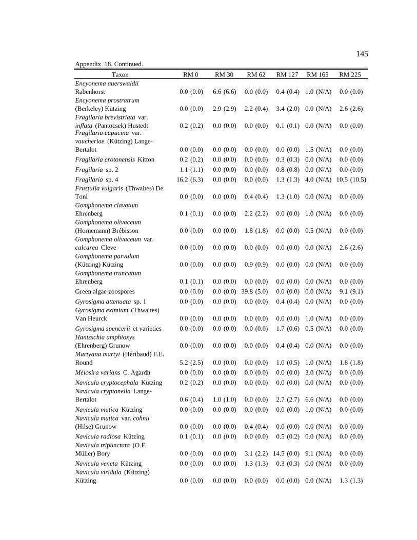
145
TaxonEncyonema auerswaldii Rabenhorst 0.0 (0.0) 6.6 (6.6) 0.0 (0.0) 0.4 (0.4) 1.0 (N/A) 0.0 (0.0)Encyonema prostratrum (Berkeley) Kützing 0.0 (0.0) 2.9 (2.9) 2.2 (0.4) 3.4 (2.0) 0.0 (N/A) 2.6 (2.6)Fragilaria brevistriata var. inflata (Pantocsek) Hustedt 0.2 (0.2) 0.0 (0.0) 0.0 (0.0) 0.1 (0.1) 0.0 (N/A) 0.0 (0.0)Fragilaria capucina var. vaucheriae (Kützing) Lange-Bertalot 0.0 (0.0) 0.0 (0.0) 0.0 (0.0) 0.0 (0.0) 1.5 (N/A) 0.0(0.0)
Fragilaria crotonensis Kitton 0.2 (0.2) 0.0 (0.0) 0.0 (0.0) 0.3 (0.3) 0.0 (N/A) 0.0 (0.0)
Fragilaria sp. 2 1.1 (1.1) 0.0 (0.0) 0.0 (0.0) 0.8 (0.8) 0.0 (N/A) 0.0 (0.0)
Fragilaria sp. 4 16.2 (6.3) 0.0 (0.0) 0.0 (0.0) 1.3 (1.3) 4.0 (N/A) 10.5 (10.5)Frustulia vulgaris (Thwaites) De Toni 0.0 (0.0) 0.0 (0.0) 0.4 (0.4) 1.3 (1.0) 0.0 (N/A) 0.0 (0.0)Gomphonema clavatum Ehrenberg 0.1 (0.1) 0.0 (0.0) 2.2 (2.2) 0.0 (0.0) 1.0 (N/A) 0.0 (0.0)Gomphonema olivaceum (Hornemann) Brébisson 0.0 (0.0) 0.0 (0.0) 1.8 (1.8) 0.0 (0.0) 0.5 (N/A) 0.0 (0.0)Gomphonema olivaceum var. calcarea Cleve 0.0 (0.0) 0.0 (0.0) 0.0 (0.0) 0.0 (0.0) 0.0 (N/A) 2.6 (2.6)Gomphonema parvulum (Kützing) Kützing 0.0 (0.0) 0.0 (0.0) 0.9 (0.9) 0.0 (0.0) 0.0 (N/A) 0.0 (0.0)Gomphonema truncatum Ehrenberg 0.1 (0.1) 0.0 (0.0) 0.0 (0.0) 0.0 (0.0) 0.0 (N/A) 0.0 (0.0)
Green algae zoospores 0.0 (0.0) 0.0 (0.0) 39.8 (5.0) 0.0 (0.0) 0.0 (N/A) 9.1 (9.1)
Gyrosigma attenuata sp. 1 0.0 (0.0) 0.0 (0.0) 0.0 (0.0) 0.4 (0.4) 0.0 (N/A) 0.0 (0.0)Gyrosigma eximium (Thwaites) Van Heurck 0.0 (0.0) 0.0 (0.0) 0.0 (0.0) 0.0 (0.0) 1.0 (N/A)0.0 (0.0)
Gyrosigma spencerii et varieties 0.0 (0.0) 0.0 (0.0) 0.0 (0.0) 1.7 (0.6) 0.5 (N/A) 0.0 (0.0)Hantzschia amphioxys (Ehrenberg) Grunow 0.0 (0.0) 0.0 (0.0) 0.0 (0.0) 0.4 (0.4)0.0 (N/A) 0.0 (0.0)Martyana martyi (Héribaud) F.E. Round 5.2 (2.5) 0.0 (0.0) 0.0 (0.0) 1.0 (0.5) 1.0 (N/A) 1.8 (1.8)
Melosira varians C. Agardh 0.0 (0.0) 0.0 (0.0) 0.0 (0.0) 0.0 (0.0) 3.0 (N/A) 0.0 (0.0)
Navicula cryptocephala Kützing 0.2 (0.2) 0.0 (0.0) 0.0 (0.0) 0.0 (0.0) 0.0 (N/A) 0.0 (0.0)Navicula cryptonella Lange-Bertalot 0.6 (0.4) 1.0 (1.0) 0.0 (0.0) 2.7 (2.7) 6.6 (N/A) 0.0(0.0)
Navicula mutica Kützing 0.0 (0.0) 0.0 (0.0) 0.0 (0.0) 0.0 (0.0) 1.0 (N/A) 0.0 (0.0)Navicula mutica var. cohnii (Hilse) Grunow 0.0 (0.0) 0.0 (0.0) 0.4 (0.4) 0.0 (0.0) 0.0 (N/A) 0.0 (0.0)
Navicula radiosa Kützing 0.1 (0.1) 0.0 (0.0) 0.0 (0.0) 0.5 (0.2) 0.0 (N/A) 0.0 (0.0)Navicula tripunctata (O.F. Müller) Bory 0.0 (0.0) 0.0 (0.0) 3.1 (2.2) 14.5 (0.0) 9.1 (N/A) 0.0 (0.0)
Navicula veneta Kützing 0.0 (0.0) 0.0 (0.0) 1.3 (1.3) 0.3 (0.3) 0.0 (N/A) 0.0 (0.0)Navicula viridula (Kützing) Kützing 0.0 (0.0) 0.0 (0.0) 0.0 (0.0) 0.0 (0.0) 0.0 (N/A) 1.3 (1.3)
Appendix 18. Continued.
RM 0 RM 30 RM 62 RM 127 RM 165 RM 225
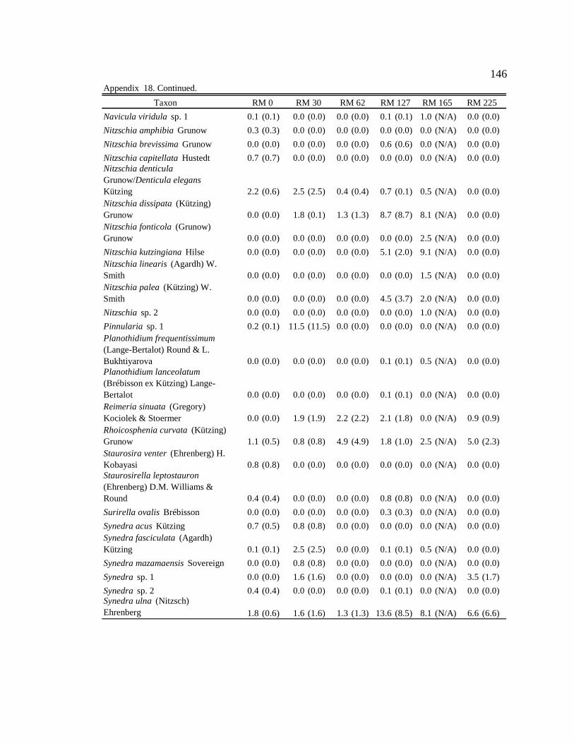
146
Taxon
Navicula viridula sp. 1 0.1 (0.1) 0.0 (0.0) 0.0 (0.0) 0.1 (0.1) 1.0 (N/A) 0.0 (0.0)
Nitzschia amphibia Grunow 0.3 (0.3) 0.0 (0.0) 0.0 (0.0) 0.0 (0.0) 0.0 (N/A) 0.0 (0.0)
Nitzschia brevissima Grunow 0.0 (0.0) 0.0 (0.0) 0.0 (0.0) 0.6 (0.6) 0.0 (N/A) 0.0 (0.0)
Nitzschia capitellata Hustedt 0.7 (0.7) 0.0 (0.0) 0.0 (0.0) 0.0 (0.0) 0.0 (N/A) 0.0 (0.0)Nitzschia denticula Grunow/Denticula elegans Kützing 2.2 (0.6) 2.5 (2.5) 0.4 (0.4) 0.7 (0.1) 0.5 (N/A) 0.0 (0.0)Nitzschia dissipata (Kützing) Grunow 0.0 (0.0) 1.8 (0.1) 1.3 (1.3) 8.7 (8.7) 8.1 (N/A) 0.0 (0.0)Nitzschia fonticola (Grunow) Grunow 0.0 (0.0) 0.0 (0.0) 0.0 (0.0) 0.0 (0.0) 2.5 (N/A) 0.0 (0.0)
Nitzschia kutzingiana Hilse 0.0 (0.0) 0.0 (0.0) 0.0 (0.0) 5.1 (2.0) 9.1 (N/A) 0.0 (0.0)Nitzschia linearis (Agardh) W. Smith 0.0 (0.0) 0.0 (0.0) 0.0 (0.0) 0.0 (0.0) 1.5 (N/A) 0.0 (0.0)Nitzschia palea (Kützing) W. Smith 0.0 (0.0) 0.0 (0.0) 0.0 (0.0) 4.5 (3.7) 2.0 (N/A) 0.0 (0.0)
Nitzschia sp. 2 0.0 (0.0) 0.0 (0.0) 0.0 (0.0) 0.0 (0.0) 1.0 (N/A) 0.0 (0.0)
Pinnularia sp. 1 0.2 (0.1) 11.5 (11.5) 0.0 (0.0) 0.0 (0.0) 0.0 (N/A) 0.0 (0.0)Planothidium frequentissimum (Lange-Bertalot) Round & L. Bukhtiyarova 0.0 (0.0) 0.0 (0.0) 0.0 (0.0) 0.1 (0.1) 0.5 (N/A) 0.0 (0.0)Planothidium lanceolatum (Brébisson ex Kützing) Lange-Bertalot 0.0 (0.0) 0.0 (0.0) 0.0 (0.0) 0.1 (0.1) 0.0 (N/A) 0.0(0.0)Reimeria sinuata (Gregory) Kociolek & Stoermer 0.0 (0.0) 1.9 (1.9) 2.2 (2.2) 2.1 (1.8) 0.0 (N/A) 0.9 (0.9)Rhoicosphenia curvata (Kützing) Grunow 1.1 (0.5) 0.8 (0.8) 4.9 (4.9) 1.8 (1.0) 2.5 (N/A) 5.0 (2.3)Staurosira venter (Ehrenberg) H. Kobayasi 0.8 (0.8) 0.0 (0.0) 0.0 (0.0) 0.0 (0.0) 0.0 (N/A) 0.0(0.0)Staurosirella leptostauron (Ehrenberg) D.M. Williams & Round 0.4 (0.4) 0.0 (0.0) 0.0 (0.0) 0.8 (0.8) 0.0 (N/A) 0.0 (0.0)
Surirella ovalis Brébisson 0.0 (0.0) 0.0 (0.0) 0.0 (0.0) 0.3 (0.3) 0.0 (N/A) 0.0 (0.0)
Synedra acus Kützing 0.7 (0.5) 0.8 (0.8) 0.0 (0.0) 0.0 (0.0) 0.0 (N/A) 0.0(0.0)Synedra fasciculata (Agardh) Kützing 0.1 (0.1) 2.5 (2.5) 0.0 (0.0) 0.1 (0.1) 0.5 (N/A) 0.0 (0.0)
Synedra mazamaensis Sovereign 0.0 (0.0) 0.8 (0.8) 0.0 (0.0) 0.0 (0.0) 0.0 (N/A) 0.0 (0.0)
Synedra sp. 1 0.0 (0.0) 1.6 (1.6) 0.0 (0.0) 0.0 (0.0) 0.0 (N/A) 3.5 (1.7)
Synedra sp. 2 0.4 (0.4) 0.0 (0.0) 0.0 (0.0) 0.1 (0.1) 0.0 (N/A) 0.0 (0.0)Synedra ulna (Nitzsch) Ehrenberg 1.8 (0.6) 1.6 (1.6) 1.3 (1.3) 13.6 (8.5) 8.1 (N/A) 6.6 (6.6)
Appendix 18. Continued.
RM 0 RM 30 RM 62 RM 127 RM 165 RM 225
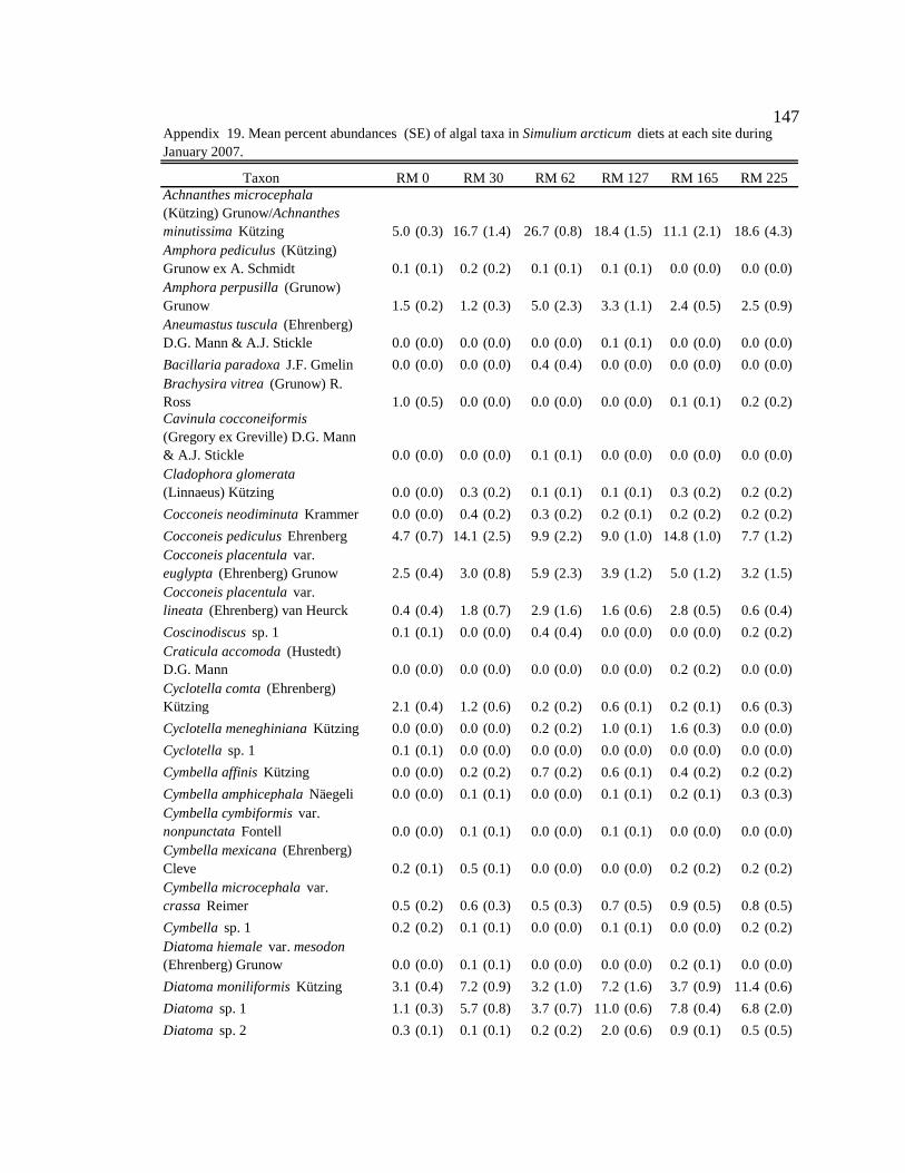
147
TaxonAchnanthes microcephala (Kützing) Grunow/Achnanthes minutissima Kützing 5.0 (0.3) 16.7 (1.4) 26.7 (0.8) 18.4 (1.5) 11.1 (2.1)18.6 (4.3)Amphora pediculus (Kützing) Grunow ex A. Schmidt 0.1 (0.1) 0.2 (0.2) 0.1 (0.1) 0.1 (0.1) 0.0 (0.0) 0.0 (0.0)Amphora perpusilla (Grunow) Grunow 1.5 (0.2) 1.2 (0.3) 5.0 (2.3) 3.3 (1.1) 2.4 (0.5) 2.5 (0.9)Aneumastus tuscula (Ehrenberg) D.G. Mann & A.J. Stickle 0.0 (0.0) 0.0 (0.0) 0.0 (0.0) 0.1(0.1) 0.0 (0.0) 0.0 (0.0)
Bacillaria paradoxa J.F. Gmelin 0.0 (0.0) 0.0 (0.0) 0.4 (0.4) 0.0 (0.0) 0.0 (0.0) 0.0 (0.0)Brachysira vitrea (Grunow) R. Ross 1.0 (0.5) 0.0 (0.0) 0.0 (0.0) 0.0 (0.0) 0.1 (0.1) 0.2 (0.2)Cavinula cocconeiformis (Gregory ex Greville) D.G. Mann & A.J. Stickle 0.0 (0.0) 0.0 (0.0) 0.1 (0.1) 0.0 (0.0) 0.0 (0.0) 0.0 (0.0)Cladophora glomerata (Linnaeus) Kützing 0.0 (0.0) 0.3 (0.2) 0.1 (0.1) 0.1 (0.1) 0.3 (0.2) 0.2 (0.2)
Cocconeis neodiminuta Krammer 0.0 (0.0) 0.4 (0.2) 0.3 (0.2) 0.2 (0.1) 0.2 (0.2) 0.2(0.2)
Cocconeis pediculus Ehrenberg 4.7 (0.7) 14.1 (2.5) 9.9 (2.2) 9.0 (1.0) 14.8 (1.0)7.7 (1.2)Cocconeis placentula var. euglypta (Ehrenberg) Grunow 2.5 (0.4) 3.0 (0.8) 5.9 (2.3) 3.9 (1.2)5.0 (1.2) 3.2 (1.5)Cocconeis placentula var. lineata (Ehrenberg) van Heurck 0.4 (0.4) 1.8 (0.7) 2.9 (1.6) 1.6 (0.6) 2.8 (0.5) 0.6 (0.4)
Coscinodiscus sp. 1 0.1 (0.1) 0.0 (0.0) 0.4 (0.4) 0.0 (0.0) 0.0 (0.0) 0.2 (0.2)Craticula accomoda (Hustedt) D.G. Mann 0.0 (0.0) 0.0 (0.0) 0.0 (0.0) 0.0 (0.0) 0.2 (0.2) 0.0 (0.0)Cyclotella comta (Ehrenberg) Kützing 2.1 (0.4) 1.2 (0.6) 0.2 (0.2) 0.6 (0.1) 0.2 (0.1) 0.6 (0.3)
Cyclotella meneghiniana Kützing 0.0 (0.0) 0.0 (0.0) 0.2 (0.2) 1.0 (0.1) 1.6 (0.3) 0.0 (0.0)
Cyclotella sp. 1 0.1 (0.1) 0.0 (0.0) 0.0 (0.0) 0.0 (0.0) 0.0 (0.0) 0.0 (0.0)
Cymbella affinis Kützing 0.0 (0.0) 0.2 (0.2) 0.7 (0.2) 0.6 (0.1) 0.4 (0.2) 0.2 (0.2)
Cymbella amphicephala Näegeli 0.0 (0.0) 0.1 (0.1) 0.0 (0.0) 0.1 (0.1) 0.2 (0.1) 0.3 (0.3)Cymbella cymbiformis var. nonpunctata Fontell 0.0 (0.0) 0.1 (0.1) 0.0 (0.0) 0.1 (0.1) 0.0 (0.0) 0.0(0.0)Cymbella mexicana (Ehrenberg) Cleve 0.2 (0.1) 0.5 (0.1) 0.0 (0.0) 0.0 (0.0) 0.2 (0.2) 0.2 (0.2)Cymbella microcephala var. crassa Reimer 0.5 (0.2) 0.6 (0.3) 0.5 (0.3) 0.7 (0.5) 0.9 (0.5) 0.8 (0.5)
Cymbella sp. 1 0.2 (0.2) 0.1 (0.1) 0.0 (0.0) 0.1 (0.1) 0.0 (0.0) 0.2 (0.2)Diatoma hiemale var. mesodon (Ehrenberg) Grunow 0.0 (0.0) 0.1 (0.1) 0.0 (0.0) 0.0 (0.0) 0.2 (0.1) 0.0 (0.0)
Diatoma moniliformis Kützing 3.1 (0.4) 7.2 (0.9) 3.2 (1.0) 7.2 (1.6) 3.7 (0.9) 11.4(0.6)
Diatoma sp. 1 1.1 (0.3) 5.7 (0.8) 3.7 (0.7) 11.0 (0.6) 7.8 (0.4) 6.8 (2.0)
Diatoma sp. 2 0.3 (0.1) 0.1 (0.1) 0.2 (0.2) 2.0 (0.6) 0.9 (0.1) 0.5 (0.5)
Appendix 19. Mean percent abundances (SE) of algal taxa in Simulium arcticum diets at each site during January 2007.
RM 0 RM 30 RM 62 RM 127 RM 165 RM 225
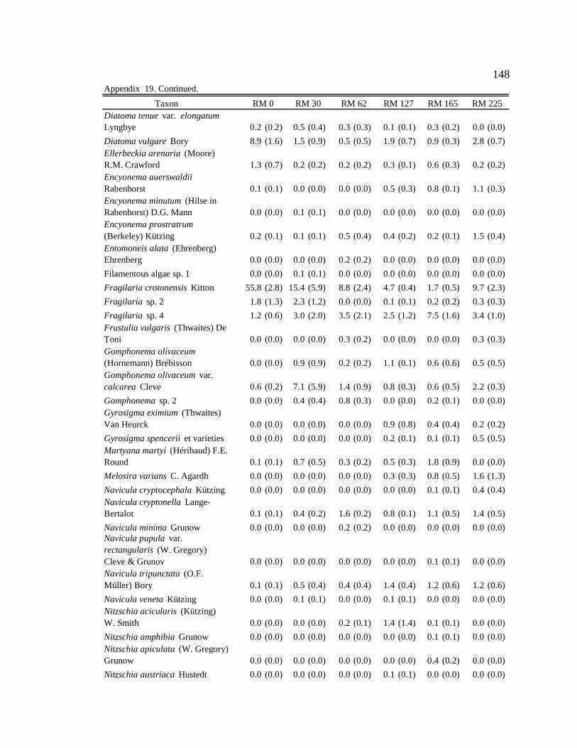
148
TaxonDiatoma tenue var. elongatum Lyngbye 0.2 (0.2) 0.5 (0.4) 0.3 (0.3) 0.1 (0.1) 0.3 (0.2) 0.0 (0.0)
Diatoma vulgare Bory 8.9 (1.6) 1.5 (0.9) 0.5 (0.5) 1.9 (0.7) 0.9 (0.3) 2.8 (0.7)Ellerbeckia arenaria (Moore) R.M. Crawford 1.3 (0.7) 0.2 (0.2) 0.2 (0.2) 0.3 (0.1) 0.6 (0.3) 0.2 (0.2)Encyonema auerswaldii Rabenhorst 0.1 (0.1) 0.0 (0.0) 0.0 (0.0) 0.5 (0.3) 0.8 (0.1) 1.1 (0.3)Encyonema minutum (Hilse in Rabenhorst) D.G. Mann 0.0 (0.0) 0.1 (0.1) 0.0 (0.0) 0.0(0.0) 0.0 (0.0) 0.0 (0.0)Encyonema prostratrum (Berkeley) Kützing 0.2 (0.1) 0.1 (0.1) 0.5 (0.4) 0.4 (0.2) 0.2 (0.1) 1.5 (0.4)Entomoneis alata (Ehrenberg) Ehrenberg 0.0 (0.0) 0.0 (0.0) 0.2 (0.2) 0.0 (0.0) 0.0 (0.0) 0.0 (0.0)
Filamentous algae sp. 1 0.0 (0.0) 0.1 (0.1) 0.0 (0.0) 0.0 (0.0) 0.0 (0.0) 0.0 (0.0)
Fragilaria crotonensis Kitton 55.8 (2.8) 15.4 (5.9) 8.8 (2.4) 4.7 (0.4) 1.7 (0.5) 9.7(2.3)
Fragilaria sp. 2 1.8 (1.3) 2.3 (1.2) 0.0 (0.0) 0.1 (0.1) 0.2 (0.2) 0.3 (0.3)
Fragilaria sp. 4 1.2 (0.6) 3.0 (2.0) 3.5 (2.1) 2.5 (1.2) 7.5 (1.6) 3.4 (1.0)Frustulia vulgaris (Thwaites) De Toni 0.0 (0.0) 0.0 (0.0) 0.3 (0.2) 0.0 (0.0) 0.0 (0.0) 0.3 (0.3)Gomphonema olivaceum (Hornemann) Brébisson 0.0 (0.0) 0.9 (0.9) 0.2 (0.2) 1.1 (0.1) 0.6 (0.6) 0.5 (0.5)Gomphonema olivaceum var. calcarea Cleve 0.6 (0.2) 7.1 (5.9) 1.4 (0.9) 0.8 (0.3) 0.6 (0.5) 2.2 (0.3)
Gomphonema sp. 2 0.0 (0.0) 0.4 (0.4) 0.8 (0.3) 0.0 (0.0) 0.2 (0.1) 0.0 (0.0)Gyrosigma eximium (Thwaites) Van Heurck 0.0 (0.0) 0.0 (0.0) 0.0 (0.0) 0.9 (0.8) 0.4 (0.4)0.2 (0.2)
Gyrosigma spencerii et varieties 0.0 (0.0) 0.0 (0.0) 0.0 (0.0) 0.2 (0.1) 0.1 (0.1) 0.5 (0.5)Martyana martyi (Héribaud) F.E. Round 0.1 (0.1) 0.7 (0.5) 0.3 (0.2) 0.5 (0.3) 1.8 (0.9) 0.0 (0.0)
Melosira varians C. Agardh 0.0 (0.0) 0.0 (0.0) 0.0 (0.0) 0.3 (0.3) 0.8 (0.5) 1.6 (1.3)
Navicula cryptocephala Kützing 0.0 (0.0) 0.0 (0.0) 0.0 (0.0) 0.0 (0.0) 0.1 (0.1) 0.4(0.4)Navicula cryptonella Lange-Bertalot 0.1 (0.1) 0.4 (0.2) 1.6 (0.2) 0.8 (0.1) 1.1 (0.5) 1.4(0.5)
Navicula minima Grunow 0.0 (0.0) 0.0 (0.0) 0.2 (0.2) 0.0 (0.0) 0.0 (0.0) 0.0 (0.0)Navicula pupula var. rectangularis (W. Gregory) Cleve & Grunov 0.0 (0.0) 0.0 (0.0) 0.0 (0.0) 0.0 (0.0) 0.1 (0.1) 0.0 (0.0)Navicula tripunctata (O.F. Müller) Bory 0.1 (0.1) 0.5 (0.4) 0.4 (0.4) 1.4 (0.4) 1.2 (0.6) 1.2 (0.6)
Navicula veneta Kützing 0.0 (0.0) 0.1 (0.1) 0.0 (0.0) 0.1 (0.1) 0.0 (0.0) 0.0 (0.0)Nitzschia acicularis (Kützing) W. Smith 0.0 (0.0) 0.0 (0.0) 0.2 (0.1) 1.4 (1.4) 0.1 (0.1) 0.0 (0.0)
Nitzschia amphibia Grunow 0.0 (0.0) 0.0 (0.0) 0.0 (0.0) 0.0 (0.0) 0.1 (0.1) 0.0 (0.0)Nitzschia apiculata (W. Gregory) Grunow 0.0 (0.0) 0.0 (0.0) 0.0 (0.0) 0.0 (0.0) 0.4 (0.2) 0.0 (0.0)
Nitzschia austriaca Hustedt 0.0 (0.0) 0.0 (0.0) 0.0 (0.0) 0.1 (0.1) 0.0 (0.0) 0.0 (0.0)
Appendix 19. Continued.
RM 0 RM 30 RM 62 RM 127 RM 165 RM 225
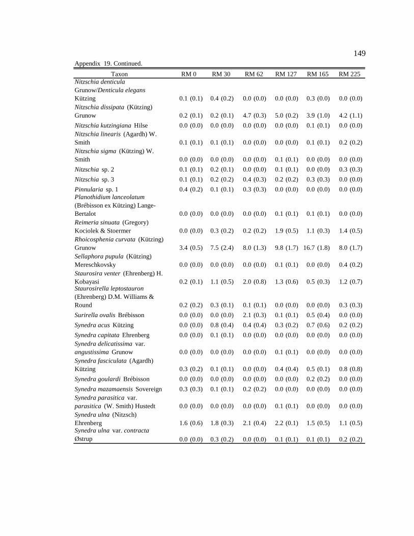
149
TaxonNitzschia denticula Grunow/Denticula elegans Kützing 0.1 (0.1) 0.4 (0.2) 0.0 (0.0) 0.0 (0.0) 0.3 (0.0) 0.0(0.0)Nitzschia dissipata (Kützing) Grunow 0.2 (0.1) 0.2 (0.1) 4.7 (0.3) 5.0 (0.2) 3.9 (1.0) 4.2 (1.1)
Nitzschia kutzingiana Hilse 0.0 (0.0) 0.0 (0.0) 0.0 (0.0) 0.0 (0.0) 0.1 (0.1) 0.0 (0.0)Nitzschia linearis (Agardh) W. Smith 0.1 (0.1) 0.1 (0.1) 0.0 (0.0) 0.0 (0.0) 0.1 (0.1) 0.2 (0.2)Nitzschia sigma (Kützing) W. Smith 0.0 (0.0) 0.0 (0.0) 0.0 (0.0) 0.1 (0.1) 0.0 (0.0) 0.0 (0.0)
Nitzschia sp. 2 0.1 (0.1) 0.2 (0.1) 0.0 (0.0) 0.1 (0.1) 0.0 (0.0) 0.3 (0.3)
Nitzschia sp. 3 0.1 (0.1) 0.2 (0.2) 0.4 (0.3) 0.2 (0.2) 0.3 (0.3) 0.0 (0.0)
Pinnularia sp. 1 0.4 (0.2) 0.1 (0.1) 0.3 (0.3) 0.0 (0.0) 0.0 (0.0) 0.0 (0.0)Planothidium lanceolatum (Brébisson ex Kützing) Lange-Bertalot 0.0 (0.0) 0.0 (0.0) 0.0 (0.0) 0.1 (0.1) 0.1 (0.1) 0.0(0.0)Reimeria sinuata (Gregory) Kociolek & Stoermer 0.0 (0.0) 0.3 (0.2) 0.2 (0.2) 1.9 (0.5) 1.1 (0.3) 1.4 (0.5)Rhoicosphenia curvata (Kützing) Grunow 3.4 (0.5) 7.5 (2.4) 8.0 (1.3) 9.8 (1.7) 16.7 (1.8) 8.0 (1.7)Sellaphora pupula (Kützing) Mereschkovsky 0.0 (0.0) 0.0 (0.0) 0.0 (0.0) 0.1 (0.1) 0.0 (0.0) 0.4 (0.2)Staurosira venter (Ehrenberg) H. Kobayasi 0.2 (0.1) 1.1 (0.5) 2.0 (0.8) 1.3 (0.6) 0.5 (0.3) 1.2(0.7)Staurosirella leptostauron (Ehrenberg) D.M. Williams & Round 0.2 (0.2) 0.3 (0.1) 0.1 (0.1) 0.0 (0.0) 0.0 (0.0) 0.3 (0.3)
Surirella ovalis Brébisson 0.0 (0.0) 0.0 (0.0) 2.1 (0.3) 0.1 (0.1) 0.5 (0.4)0.0 (0.0)
Synedra acus Kützing 0.0 (0.0) 0.8 (0.4) 0.4 (0.4) 0.3 (0.2) 0.7 (0.6) 0.2(0.2)
Synedra capitata Ehrenberg 0.0 (0.0) 0.1 (0.1) 0.0 (0.0) 0.0 (0.0) 0.0 (0.0) 0.0 (0.0)Synedra delicatissima var. angustissima Grunow 0.0 (0.0) 0.0 (0.0) 0.0 (0.0) 0.1 (0.1) 0.0 (0.0) 0.0 (0.0)Synedra fasciculata (Agardh) Kützing 0.3 (0.2) 0.1 (0.1) 0.0 (0.0) 0.4 (0.4) 0.5 (0.1) 0.8 (0.8)
Synedra goulardi Brébisson 0.0 (0.0) 0.0 (0.0) 0.0 (0.0) 0.0 (0.0) 0.2 (0.2)0.0 (0.0)
Synedra mazamaensis Sovereign 0.3 (0.3) 0.1 (0.1) 0.2 (0.2) 0.0 (0.0) 0.0 (0.0) 0.0 (0.0)Synedra parasitica var. parasitica (W. Smith) Hustedt 0.0 (0.0) 0.0 (0.0) 0.0 (0.0) 0.1 (0.1)0.0 (0.0) 0.0 (0.0)Synedra ulna (Nitzsch) Ehrenberg 1.6 (0.6) 1.8 (0.3) 2.1 (0.4) 2.2 (0.1) 1.5 (0.5) 1.1 (0.5)Synedra ulna var. contracta Østrup 0.0 (0.0) 0.3 (0.2) 0.0 (0.0) 0.1 (0.1) 0.1 (0.1) 0.2 (0.2)
Appendix 19. Continued.
RM 0 RM 30 RM 62 RM 127 RM 165 RM 225
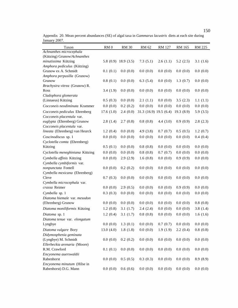
150
TaxonAchnanthes microcephala (Kützing) Grunow/Achnanthes minutissima Kützing 5.8 (0.9) 18.9 (3.5) 7.3 (5.1) 2.6 (1.1) 5.2 (2.5) 3.1(1.6)Amphora pediculus (Kützing) Grunow ex A. Schmidt 0.1 (0.1) 0.0 (0.0) 0.0 (0.0) 0.0 (0.0) 0.0 (0.0) 0.0 (0.0)Amphora perpusilla (Grunow) Grunow 0.8 (0.1) 0.0 (0.0) 6.3 (5.4) 0.0 (0.0) 1.3 (0.7) 0.0 (0.0)Brachysira vitrea (Grunow) R. Ross 3.4 (1.9) 0.0 (0.0) 0.0 (0.0) 0.0 (0.0) 0.0 (0.0) 0.0 (0.0)Cladophora glomerata (Linnaeus) Kützing 0.5 (0.3) 0.0 (0.0) 2.1 (1.1) 0.0 (0.0) 3.5 (2.3) 1.1 (1.1)
Cocconeis neodiminuta Krammer 0.0 (0.0) 0.2 (0.2) 0.0 (0.0) 0.0 (0.0) 0.0 (0.0) 0.0(0.0)
Cocconeis pediculus Ehrenberg 17.6 (1.0) 2.4 (0.0) 31.3 (16.9) 19.5 (6.4) 19.3 (8.9) 5.9 (3.5)Cocconeis placentula var. euglypta (Ehrenberg) Grunow 2.8 (1.4) 2.7 (0.8) 0.8 (0.8) 4.4 (3.0)0.9 (0.9) 2.8 (2.3)Cocconeis placentula var. lineata (Ehrenberg) van Heurck 1.2 (0.4) 0.0 (0.0) 4.9 (3.8) 0.7 (0.7) 0.5 (0.5) 1.2 (0.7)
Coscinodiscus sp. 1 0.0 (0.0) 0.0 (0.0) 0.0 (0.0) 0.0 (0.0) 0.0 (0.0) 0.4 (0.4)Cyclotella comta (Ehrenberg) Kützing 0.5 (0.1) 0.0 (0.0) 0.8 (0.8) 0.0 (0.0) 0.0 (0.0) 0.0 (0.0)
Cyclotella meneghiniana Kützing 0.0 (0.0) 0.0 (0.0) 0.8 (0.8) 0.7 (0.7) 0.0 (0.0) 0.0 (0.0)
Cymbella affinis Kützing 0.0 (0.0) 2.9 (2.9) 1.6 (0.8) 0.0 (0.0) 0.9 (0.9) 0.0 (0.0)Cymbella cymbiformis var. nonpunctata Fontell 0.0 (0.0) 0.2 (0.2) 0.0 (0.0) 0.0 (0.0) 0.0 (0.0) 0.0(0.0)Cymbella mexicana (Ehrenberg) Cleve 0.7 (0.3) 0.0 (0.0) 0.0 (0.0) 0.0 (0.0) 0.0 (0.0) 0.0 (0.0)Cymbella microcephala var. crassa Reimer 0.0 (0.0) 2.9 (0.5) 0.0 (0.0) 0.0 (0.0) 0.9 (0.9) 0.0 (0.0)
Cymbella sp. 1 0.3 (0.3) 0.0 (0.0) 0.0 (0.0) 0.0 (0.0) 0.0 (0.0) 0.0 (0.0)Diatoma hiemale var. mesodon (Ehrenberg) Grunow 0.0 (0.0) 0.0 (0.0) 0.0 (0.0) 0.0 (0.0) 0.0 (0.0) 0.8 (0.8)
Diatoma moniliformis Kützing 1.2 (0.8) 3.1 (1.7) 2.4 (2.4) 0.0 (0.0) 0.0 (0.0) 3.8 (1.4)
Diatoma sp. 1 1.2 (0.4) 3.1 (1.7) 0.8 (0.8) 0.0 (0.0) 0.0 (0.0) 1.6 (1.6)Diatoma tenue var. elongatum Lyngbye 0.0 (0.0) 1.3 (0.1) 0.0 (0.0) 0.7 (0.7) 0.0 (0.0) 0.0 (0.0)
Diatoma vulgare Bory 13.0 (4.0) 1.8 (1.8) 0.0 (0.0) 1.9 (1.9) 2.2 (0.4) 0.8 (0.8)Didymosphenia geminata (Lyngbye) M. Schmidt 0.0 (0.0) 0.2 (0.2) 0.0 (0.0) 0.0 (0.0) 0.0 (0.0) 0.0 (0.0)Ellerbeckia arenaria (Moore) R.M. Crawford 0.1 (0.1) 0.0 (0.0) 0.0 (0.0) 0.0 (0.0) 0.0 (0.0) 0.0 (0.0)Encyonema auerswaldii Rabenhorst 0.0 (0.0) 0.5 (0.5) 0.3 (0.3) 0.0 (0.0) 0.0 (0.0) 8.9 (8.9)Encyonema minutum (Hilse in Rabenhorst) D.G. Mann 0.0 (0.0) 0.6 (0.6) 0.0 (0.0) 0.0(0.0) 0.0 (0.0) 0.0 (0.0)
Appendix 20. Mean percent abundances (SE) of algal taxa in Gammarus lacustris diets at each site during January 2007.
RM 0 RM 30 RM 62 RM 127 RM 165 RM 225
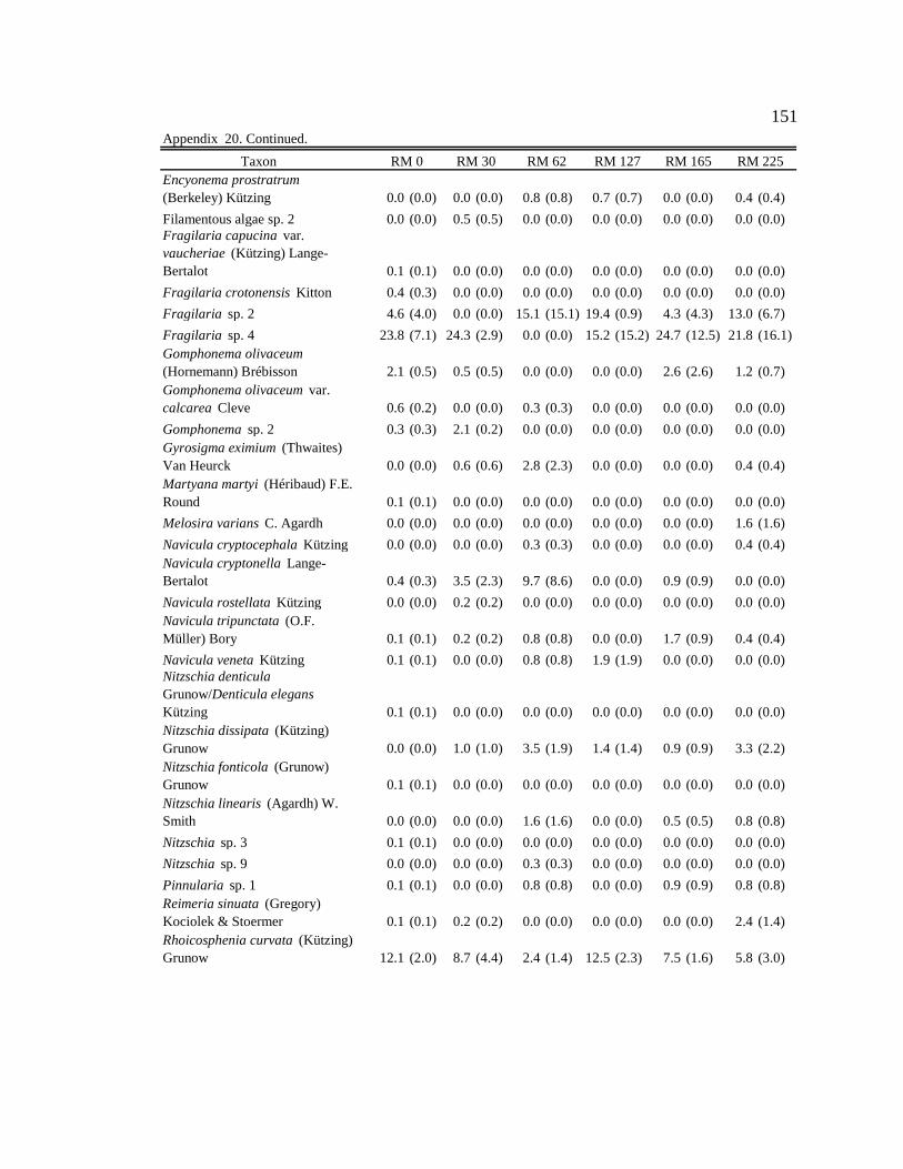
151
TaxonEncyonema prostratrum (Berkeley) Kützing 0.0 (0.0) 0.0 (0.0) 0.8 (0.8) 0.7 (0.7) 0.0 (0.0) 0.4 (0.4)
Filamentous algae sp. 2 0.0 (0.0) 0.5 (0.5) 0.0 (0.0) 0.0 (0.0) 0.0 (0.0) 0.0 (0.0)Fragilaria capucina var. vaucheriae (Kützing) Lange-Bertalot 0.1 (0.1) 0.0 (0.0) 0.0 (0.0) 0.0 (0.0) 0.0 (0.0) 0.0 (0.0)
Fragilaria crotonensis Kitton 0.4 (0.3) 0.0 (0.0) 0.0 (0.0) 0.0 (0.0) 0.0 (0.0) 0.0 (0.0)
Fragilaria sp. 2 4.6 (4.0) 0.0 (0.0) 15.1 (15.1) 19.4 (0.9) 4.3 (4.3) 13.0 (6.7)
Fragilaria sp. 4 23.8 (7.1) 24.3 (2.9) 0.0 (0.0) 15.2 (15.2) 24.7 (12.5) 21.8 (16.1)Gomphonema olivaceum (Hornemann) Brébisson 2.1 (0.5) 0.5 (0.5) 0.0 (0.0) 0.0 (0.0) 2.6 (2.6) 1.2 (0.7)Gomphonema olivaceum var. calcarea Cleve 0.6 (0.2) 0.0 (0.0) 0.3 (0.3) 0.0 (0.0) 0.0 (0.0) 0.0 (0.0)
Gomphonema sp. 2 0.3 (0.3) 2.1 (0.2) 0.0 (0.0) 0.0 (0.0) 0.0 (0.0) 0.0 (0.0)Gyrosigma eximium (Thwaites) Van Heurck 0.0 (0.0) 0.6 (0.6) 2.8 (2.3) 0.0 (0.0) 0.0 (0.0) 0.4 (0.4)Martyana martyi (Héribaud) F.E. Round 0.1 (0.1) 0.0 (0.0) 0.0 (0.0) 0.0 (0.0) 0.0 (0.0) 0.0 (0.0)
Melosira varians C. Agardh 0.0 (0.0) 0.0 (0.0) 0.0 (0.0) 0.0 (0.0) 0.0 (0.0) 1.6 (1.6)
Navicula cryptocephala Kützing 0.0 (0.0) 0.0 (0.0) 0.3 (0.3) 0.0 (0.0) 0.0 (0.0) 0.4 (0.4)Navicula cryptonella Lange-Bertalot 0.4 (0.3) 3.5 (2.3) 9.7 (8.6) 0.0 (0.0) 0.9 (0.9) 0.0 (0.0)
Navicula rostellata Kützing 0.0 (0.0) 0.2 (0.2) 0.0 (0.0) 0.0 (0.0) 0.0 (0.0) 0.0 (0.0)Navicula tripunctata (O.F. Müller) Bory 0.1 (0.1) 0.2 (0.2) 0.8 (0.8) 0.0 (0.0) 1.7 (0.9) 0.4 (0.4)
Navicula veneta Kützing 0.1 (0.1) 0.0 (0.0) 0.8 (0.8) 1.9 (1.9) 0.0 (0.0) 0.0 (0.0)Nitzschia denticula Grunow/Denticula elegans Kützing 0.1 (0.1) 0.0 (0.0) 0.0 (0.0) 0.0 (0.0) 0.0 (0.0) 0.0 (0.0)Nitzschia dissipata (Kützing) Grunow 0.0 (0.0) 1.0 (1.0) 3.5 (1.9) 1.4 (1.4) 0.9 (0.9) 3.3 (2.2)Nitzschia fonticola (Grunow) Grunow 0.1 (0.1) 0.0 (0.0) 0.0 (0.0) 0.0 (0.0) 0.0 (0.0) 0.0 (0.0)Nitzschia linearis (Agardh) W. Smith 0.0 (0.0) 0.0 (0.0) 1.6 (1.6) 0.0 (0.0) 0.5 (0.5) 0.8 (0.8)
Nitzschia sp. 3 0.1 (0.1) 0.0 (0.0) 0.0 (0.0) 0.0 (0.0) 0.0 (0.0) 0.0 (0.0)
Nitzschia sp. 9 0.0 (0.0) 0.0 (0.0) 0.3 (0.3) 0.0 (0.0) 0.0 (0.0) 0.0 (0.0)
Pinnularia sp. 1 0.1 (0.1) 0.0 (0.0) 0.8 (0.8) 0.0 (0.0) 0.9 (0.9) 0.8 (0.8)Reimeria sinuata (Gregory) Kociolek & Stoermer 0.1 (0.1) 0.2 (0.2) 0.0 (0.0) 0.0 (0.0) 0.0 (0.0) 2.4 (1.4)Rhoicosphenia curvata (Kützing) Grunow 12.1 (2.0) 8.7 (4.4) 2.4 (1.4) 12.5 (2.3) 7.5 (1.6) 5.8 (3.0)
Appendix 20. Continued.
RM 0 RM 30 RM 62 RM 127 RM 165 RM 225
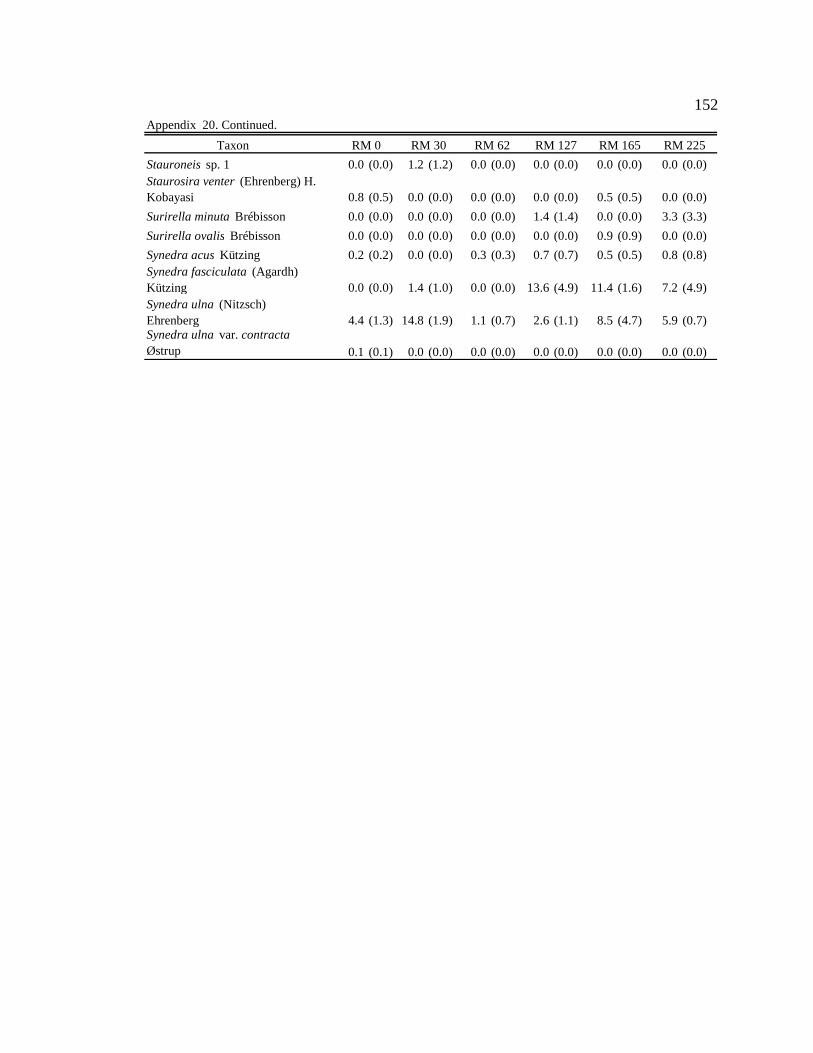
152
Taxon
Stauroneis sp. 1 0.0 (0.0) 1.2 (1.2) 0.0 (0.0) 0.0 (0.0) 0.0 (0.0) 0.0 (0.0)Staurosira venter (Ehrenberg) H. Kobayasi 0.8 (0.5) 0.0 (0.0) 0.0 (0.0) 0.0 (0.0) 0.5 (0.5) 0.0(0.0)
Surirella minuta Brébisson 0.0 (0.0) 0.0 (0.0) 0.0 (0.0) 1.4 (1.4) 0.0 (0.0) 3.3 (3.3)
Surirella ovalis Brébisson 0.0 (0.0) 0.0 (0.0) 0.0 (0.0) 0.0 (0.0) 0.9 (0.9) 0.0 (0.0)
Synedra acus Kützing 0.2 (0.2) 0.0 (0.0) 0.3 (0.3) 0.7 (0.7) 0.5 (0.5) 0.8 (0.8)Synedra fasciculata (Agardh) Kützing 0.0 (0.0) 1.4 (1.0) 0.0 (0.0) 13.6 (4.9) 11.4 (1.6) 7.2 (4.9)Synedra ulna (Nitzsch) Ehrenberg 4.4 (1.3) 14.8 (1.9) 1.1 (0.7) 2.6 (1.1) 8.5 (4.7) 5.9 (0.7)Synedra ulna var. contracta Østrup 0.1 (0.1) 0.0 (0.0) 0.0 (0.0) 0.0 (0.0) 0.0 (0.0) 0.0 (0.0)
Appendix 20. Continued.
RM 0 RM 30 RM 62 RM 127 RM 165 RM 225

153
REFERENCES
Abelho, M. 2001. From litterfall to breakdown in streams: a review. The Scientific World 1: 656-680.
Allan, J. D., and A. S. Flecker. 1993. Biodiversity conservation in running waters.
Bioscience 43: 32-43. Angradi, T. 1991. Transport of coarse particulate organic matter in an Idaho river, USA.
Hydrobiologia 211:171-183. Angradi, T. R. 1994. Trophic linkages in the lower Colorado River: multiple stable
isotope evidence. Journal of North American Benthological Society 13:479-495. Armitage, P. D., and M. H. Capper. 1976. The numbers, biomass and transport
downstream of micro-crustaceans and Hydra from Cow Green Reservoir (Upper Teesdale). Freshwater biology 6:425–432.
Arscott, D., K. Tockner, and J. Ward. 2001. Thermal heterogeneity along a braided
floodplain river (Tagliamento River, northeastern Italy). Canadian Journal of Fisheries and Aquatic Sciences 58:2359-2373.
Arsuffi, T. L., and K. Suberkropp. 1989. Selective feeding by shredders on leaf-
colonizing stream fungi: comparison of macroinvertebrate taxa. Oecologia 79:30-37.
Barber, L. B., S. H. Keefe, R. C. Antweiler, H. E. Taylor, and R. D. Wass. 2006.
Accumulation of contaminants in fish from wastewater treatment wetlands. Environmental Science & Technology 40:603-611.
Bärlocher, F. 1985. The role of fungi in the nutrition of stream invertebrates. Botanical
Journal of the Linnean Society 91:83-94. Bastow, J., J. Sabo, J. Finlay, and M. Power. 2002. A basal aquatic-terrestrial trophic link
in rivers: algal subsidies via shore-dwelling grasshoppers. Oecologia 131:261-268.
154
Baxter, R. M. 1977. Environmental effects of dams and impoundments. Annual Review of Ecology and Systematics 8:255-283.
Baxter, C. V., K. D. Fausch, and W. Carl Saunders. 2005. Tangled webs: reciprocal flows
of invertebrate prey link streams and riparian zones. Freshwater biology 50:201-220.
Benke, A.C. 1990. A perspective on America’s vanishing streams. Journal of the North
American Benthological Society 9:77-88. Benke, A. C., and B. J. Wallace. 1980. Trophic basis of production among net-spinning
caddisflies in a southern Appalachian stream. Ecology 61:108-118. Benke, A. C., and J. B. Wallace. 1997. Trophic basis of production among riverine
caddisflies: implications for food Web analysis. Ecology 78:1132-1145. Berg, M. B. 1995. Larval food and feeding behavior. Pages 136-168 in P. D. Armitage, P.
S. Cranston, and L. C. V. Pinder, editors. The Chironomidae: The Biology and Ecology of Non-Biting Midges. Chapman and Hall, London.
Bilby, R. E., B. R. Fransen, and P. A. Bisson. 1996. Incorporation of nitrogen and carbon
from spawning coho salmon into the trophic system of small streams: evidence from stable isotopes. Canadian Journal of Fisheries and Aquatic Sciences 53:164-173.
Bird, G. A., and N. K. Kaushik. 1984. Survival and growth of early-instar nymphs of
Ephemerella subvaria fed various diets. Hydrobiologia 119:227-233. Blinn, D. W., R. Truitt, and A. Pickart. 1989. Response of epiphytic diatom communities
from the tailwaters of Glen Canyon Dam, Arizona, to elevated water temperature. Regulated Rivers: Research and Management 4:91-96.
Blinn, D. W., and G. A. Cole. 1991. Algal and invertebrate biota in the Colorado River:
comparison of pre-and post-dam conditions. Pages 102-123 in Colorado River Ecology and Dam Management. National Academy Press, Washington, DC.
Blinn, D. W., J. P. Shannon, L.E. Stevens, and J. P. Carder. 1994. Consequences of
fluctuating discharge for lotic communities. Journal of North American Benthological Society 14:233-248.
Blinn, D. W., J. P. Shannon, P. L. Benenati, and K. P. Wilson. 1998. Algal ecology in
tailwater stream communities: the Colorado River below Glen Canyon Dam, Arizona. Journal of Phycology 34:734-740.

155
Bowen, S. H. 1984. Evidence of a detritus food chain based on consumption of organic precipitates. Bulletin of Marine Science 35:440-448.
Carlough, L. A. 1994. Origins, structure, and trophic significance of amorphous seston in
a blackwater river. Freshwater Biology 31:227–237. Carothers, S. W., and B. T. Brown. 1991. The Colorado River through Grand Canyon:
natural history and human change. The University of Arizona Press, Tucson. Chandler, D. C. 1937. Fate of typical lake plankton in streams. Ecological Monographs
7:445-479. Childs, M.R., R.W. Clakson, and A.T. Robinson. 1998. Resource use by larval and early
juvenile native fishes in the Little Colorado River, Grand Canyon, Arizona. Transactions of the American Fisheries Society 127: 620-629.
Clarke, A. D., K. H. Telmer, and J. M. Shrimpton. 2007. Using natural elemental
signatures to determine habitat use and population structure for a fluvial species, the Arctic grayling, in a watershed impacted by a large reservoir. Journal of Applied Ecology 44:1156–1165.
Crayton, W. M., and M. R. Sommerfield. 1979. Composition and abundance of
phytoplankton in tributaries of the lower Colorado River, Grand Canyon Region Hydrobiologia 66:81-94.
Cross, W.F., J.B. Wallace, and A.D. Rosemond. 2007. Nutrient enrichment reduces
constraints on material flows in a detritus-based food web. Ecology 88:2563-2575.
Cummins, K. W. 1973. Trophic relations of aquatic insects. Annual Review of
Entomology 18:183-206. Cummins, K. W., and M. J. Klug. 1979. Feeding ecology of stream invertebrates. Annual
Review of Ecology and Systematics 10:147-172. Currie, D. C., and D. A. Craig. 1987. Feeding strategies of larval black flies. Pages 155-
170 in K. C. Kim and R. W. Merritt, editors. Black Flies: Ecology, Population Management,and Annotated World List. Pennsylvania State University Press, University Park, PA.
Cushing, C. E. 1964. Plankton and water chemistry in the Montreal River lake-stream
system, Saskatchewan. Ecology 45:306-313.
156
Cushing, C. E., G. W. Minshall, and J. D. Newbold. 1993. Transport dynamics of fine particulate organic matter in two Idaho streams. Limnology and Oceanography 38:pp. 1101-1115
Czarnecki, D. B., and D. W. Blinn. 1977. Diatoms of lower Lake Powell and vicinity.
Bibliotheca Phycologica, Band 28:1-119. Czarnecki, D. B., and D. W. Blinn. 1978. Diatoms of southwestern USA 2: Diatoms of
the Colorado River in Grand Canyon National Park and vicinity. Bibliotheca Phycologica 38:182.
Czarnecki, D. B., D. W. Blinn, and T. Tompkins. 1976. A periphytic microflora analysis
of the Colorado River and major tributaries in the Grand Canyon National Park and vicinity. Colorado River Research Program. Technical Report. No.6.
Dallas, H. 2008. Water temperature and riverine ecosystems: An overview of knowledge
and approaches for assessing biotic responses, with special reference to South Africa. Water SA 34:393-403.
Decho, A. W., and D. J. W. Moriarty. 1990. Investigation of bacterial mucus-exopolymer
utilization by marine animals: methodology and results using harpacticoid copepods. Limnology and Oceanography 35:1039–1049.
Dixit, S. S., J. P. Smol, J. C. Kingston, and D. F. Charles. 1992. Diatoms: Powerful
indicators of environmental change. Environmental Science and Technology 26:22-33.
Doi, H., K.-H. Chang, T. Ando, H. Imai, S. Nakano, A. Kajimoto, and I. Katano. 2008.
Drifting plankton from a reservoir subsidize downstream food webs and alter community structure. Oecologia 156:363-371.
Edmunds, G. F., Jr. 1959. The mayflies of Glen Canyon Dam area, Colorado River, Utah.
Utah Academy Proceedings 36:79-80. Elliott, J. M., and J. Corlett. 1972. The Ecology of Morecambe Bay. IV. Invertebrate drift
into and from the River Leven. Journal of Applied Ecology 9:195-205. Enache, M., and Y. T. Prairie. 2002. WA-PLS diatom-based pH, TP and DOC inference
models from 42 lakes in the Abitibi clay belt area (Quebec, Canada). Journal of Paleolimnology 27:151-171.
Erman, D. C., and W. C. Chouteau. 1979. Fine particulate organic carbon output from
fens and its effect on benthic macroinvertebrates. Oikos 32:409-415.
157
Ferrington, L.C., Jr., M. B. Berg, and W. P. Coffman. 2008. Chironomidae. Chapter 26 in R. W. Merritt, K. W. Cummins, and M. B. Berg, editors. An Introduction to the Aquatic Insects of North America. 4th Ed. Kendall/Hunt Publishing Co., Dubuque, Iowa.
Finlay, J. C., M. E. Power, and G. Cabana. 1999. Effects of water velocity on algal
carbon isotope ratios: Implications for river food web studies. Limnology and Oceanography 44:1198-1203.
Fisher, S. G., and G. E. Likens. 1973. Energy flow in Bear Brook, New Hampshire: An
integrative approach to stream ecosystem metabolism. Ecological Monographs 43:421-439.
France, R. L. 1995a. Critical examination of stable isotope analysis as a means for tracing
carbon pathways in stream ecosystems. Canadian Journal of Fisheries and Aquatic Sciences 52:651-656.
France, R. L. 1996. Carbon-13 conundrums: limitations and cautions in the use of stable
isotope analysis in stream ecotonal research. Canadian Journal of Fisheries and Aquatic Sciences 53:1916–1919.
Friberg, N., and D. Jacobsen. 1994. Feeding plasticity of two detritivore-shredders.
Freshwater Biology 32:133-142. Gloss, S. P., and L. G. Coggins. 2005. Fishes of Grand Canyon. Pages 33-56 in S. P.
Gloss, J. E. Lovich, and T. S. Melis, editors. The state of the Colorado River ecosystem in Grand Canyon: U.S. Geological Survey Circular 1282.
Graça, M.A.S., Canhoto, C. 2006. Leaf litter processing in low order streams.Limnetica
25: 1-10. Gregory, S. V., F. J. Swanson, W. A. McKee, and K. W. Cummins. 1991. An ecosystem
perspective of riparian zones. BioScience 41:540-551. Haden, G. A., J. P. Shannon, K. P. Wilson, and D. W. Blinn. 2003. Benthic community
structure of the Green and Colorado Rivers through Canyonlands National Park, Utah, USA. Southwestern Naturalist 48:23-35.
Hall, R. O. Jr., C. L. Peredney, and J. L. Meyer. 1996. The effect of invertebrate
consumption on bacterial transport in a mountain stream. Limnology and Oceanography 41:1180-1187.
Hall, R. O., Jr., M. F. Dybdahl, and M. C. VanderLoop. 2006. Extremely high secondary
production of introduced snails in rivers. Ecological Applications 16:1121-1131.
158
Hall, R. O., Jr., G. E. Likens, and H. M. Malcom. 2001. Trophic basis of invertebrate production in 2 streams at the Hubbard Brook Experimental Forest. Journal of the North American Benthological Society 20:432-447.
Hall, R. O., Jr., J.B., Wallace, S.L. Eggert. 2000. Organic matter flow in stream food
webs with reduced detrital resource base. Ecology 8:3445-3463. Hamilton, S. K., and W. M. Lewis Jr. 1992. Stable carbon and nitrogen isotopes in algae
and detritus from the Orinoco River floodplain. Venezuela. Geochim. Cosmochim. Acta 56:4237-4246.
Hamilton, S. K., W. M. Lewis, and S. J. Sippel. 1992. Energy sources for aquatic animals
in the Orinoco River floodplain: evidence from stable isotopes. Oecologia 89:324-330.
Hardwick, G. G., D. W. Blinn, H. D. Usher, and 1992. Epiphytic diatoms on Cladophora
Glomerata in the Colorado River, Arizona: Longitudinal and vertical distribution in a regulated river. The Southwestern Naturalist 37:148-156.
Hart, D. D. 1987. Processes and patterns of competition in larval black flies. Pages 109-
128 in K. K.C. and M. R.W., editors. Black Flies: Ecology, Population Management, and Annotated World List. Pennsylvania State University Press, University Park, PA.
Hart, D. D., T. E. Johnson, K. L. Bushaw-Newton, R. J. Horwitz, A. T. Bednarek, D. F.
Charles, D. A. Kreeger, and D. J. Velinsky. 2002. Dam removal: Challenges and opportunities for ecological research and river restoration. BioScience 52:669-682.
Hart, D. D., and S. C. Latta. 1986. Determinants of ingestion rates in filter-feeding larval
black flies (Diptera: Simuliidae). Freshwater Biology 16:1-12. Hart, E. A., and J. R. Lovvorn. 2003. Algal vs. macrophyte inputs to food webs of inland
saline wetlands. Ecology 84:3317-3326. Hartman, R. T., and C. L. Himes. 1961. Phytoplankton from Pymatuning Reservoir in
downstream areas of the Shenango River. Ecology 42:180-183. Harvey, J., M. Hoy, and R. Rodriguez. 2009. Molecular detection of native and invasive
marine invertebrate larvae present in ballast and open water environmental samples collected in Puget Sound. Journal of Experimental Marine Biology and Ecology 369:93-99.
159
Haynes, A., and B. J. R. Taylor. 1984. Food finding and food preference in Potamopyrgus jenkinsi (E.A. Smith) (Gastropoda: Prosobranchia). Archiv fur Hydrobiologie 100:479-491.
Henriques-Oliveira, A. L., J. L. Nessimian, and L. F. M. Dorvillé. 2003. Feeding habits
of chironomid larvae (Insecta: Diptera) from a stream in the Floresta da Tijuca, Rio de Janeiro, Brazil. Brazilian Journal of Biology 63:269-281.
Hill, M. O., and H. G. Gauch. 1980. Detrended Correspondence Analysis: An improved
ordination technique. Vegetatio 42:47–58. Hill, M. O.1979. DECORANA — A FORTRAN program for Detrended Correspondence
Analysis and reciprocal averaging. Pages 52 in Ecology and Systematics. Cornell University, Ithaca, New York.
Hodkinson, I. D., and K. A. Williams. 1980. Tube formation and distribution of
Chironomus plumosus L. (Diptera; Chironomidae) in a eutrophic woodland pond. Pages 331-337 in D. A. Murray, editor. Chironomidae; Ecology, Systematics, Cytology, and Physiology. Pergamon Press, Oxford.
Hofnecht, G. 1981. Seasonal community dynamics of aquatic invertebrates in the
Colorado River and its tributaries within Grand Canyon, Arizona. M.S. thesis. Northern Arizona University, Flagstaff.
Hughes, D. A. 1970. Some factors affecting drift and upstream movements of Gammarus
Pulex. Ecology 51:301-305. Horvath, T. G. 2004. Retention of particulate matter by macrophytes in a first-order
stream. Aquatic Botany 78:27-36. Hynes, H. B. N. 1975. The stream and its valley. Verhandlungen der Internationalen
Vereinigung für theoretische und angewandte Limnologie 19:1-15. [ICOLD] International Commission on Large Dams. 1998. World Register of Dams. Paris: International Commission on Large Dams. Ingram, B. L., and P. K.Webber. 1999. Salmon origin in California’s Sacramento–San
Joaquin River system as determined by otolith strontium isotopic composition. Geology 27:851–854.
Kelly, D. W., J. T. A. Dick, and W. I. Montgomery. 2002. The functional role of
Gammarus (Crustacea, Amphipoda): shredders, predators, or both? Hydrobiologia 485:199-203.
160
Kelly, M. G., H. C. Bennion, E. J. Cox, B. Goldsmith, J. Jamieson, S. Juggins, D. G. Mann, and R. J. Telford. 2005. Common freshwater diatoms of Britain and Ireland: an interactive key. Environment Agency, Bristol.
Maciolek, J. A., and M. G. Tunzi. 1968. Microseston dynamics in a simple Sierra Nevada
lake-stream system.Ecology 49:60-75. Macneil, C., J. T. A. Dick, and R. W. Elwood. 1997. The trophic ecology of freshwater
Gammarus Spp. (Crustacea: Amphipoda): Problems and perspectives concerning the functional feeding group concept. Biological Reviews 72:349-364.
Mann, K. H. 1988. Production and use of detritus in various freshwater, estuarine, and
coastal marine ecosystems. Limnology and Oceanography 33:910-930. McCormick, P. V., and R. J. Stevenson. 1989. Effects of snail grazing on benthic algal
community structure in different nutrient environments. Journal of the North American Benthological Society 8:162–172.
McCormick, P. V., and R. J. Stevenson. 1991. Mechanisms of benthic algal succession in
lotic environments. Ecology 72:1835-1848. McCormick, P. V., and J. J. Cairns. 1994. Algae as indicators of environmental change.
Journal of Applied Phycology 6:509-526.
McCully, P. 1996. Silenced rivers: The ecology and politics of large dams. Zed Books Ltd.
McLachlan, A. J., A. Brennan, and R. S. Wotton. 1978. Particle size and chironomid
(Diptera) food in an upland river. Oikos 31:247-253. McMillan, G. L., and J. Verduin. 1953. Photosynthesis of natural communities dominated
by Cladophora glomerata and Ulothrix zonata. The Ohio Journal of Science 53:373-377.
Mercado-Silva, N., R. H. Matthew, and M. J. V. Zanden. 2008. The effects of
impoundment and non-native species on a river food web in Mexico's central plateau. River Research and Applications:1-19.
Merritt, R.W., K.W. Cummins, and M.B. Berg, eds. 2008. An Introduction to the Aquatic
Insects of North America. 4th Ed., Kendall/Hunt Publishing Co., Dubuque, Iowa. Miller, J., and T. Georgian. 1992. Estimation of fine particulate transport in streams using
pollen as a seston analog. Journal of the North American Benthological Society 11:172-180.
161
Minckley, W. L., P. C. Marsh, J. E. Deacon, T. E. Dowling, P. W. Hedrick, W. J. Matthews, and G. Mueller. 2003. A conservation plan for native fishes of the lower Colorado River. BioScience 53:219-232.
Monaghan, M. T., S. A. Thomas, G. W. Minshall, J. D. Newbold, and C. E. Cushing.
2001. The influence of filter-feeding benthic macroinvertebrates on the transport and deposition of particulate organic matter and diatoms in two streams. Limnology and Oceanography 46:1091-1099.
Musser, G. G. 1959. Annotated check list of aquatic insects of Glen Canyon. Appendix E.
Pages 207-211 in Ecological studies of the flora and fauna in Glen Canyon. University of Utah Anthropological Papers, Salt Lake City.
Nakano, S., H. Miyasaka, and N. Kuhara. 1999. Terrestrial-aquatic linkages: Riparian
arthropod inputs alter trophic cascades in a stream food web. Ecology 80:2435-2441.
Nakano, S., and M. Murakami. 2001. Reciprocal subsidies: Dynamic interdependence
between terrestrial and aquatic food Webs. Proceedings of the National Academy of Sciences of the United States of America 98:166-170.
Newbold, J. D., S. A. Thomas, G. W. Minshall, C. E. Cushing, and T. Georgian. 2005.
Deposition, benthic residence, and resuspension of fine organic particles in a mountain stream. Limnology and Oceanography 50:1571-1580.
Nilsson, C., and K. Berggren. 2000. Alterations of riparian ecosystems caused by river
regulation. BioScience 50:783-792. Oberlin, G. E., J. P. Shannon, and D. W. Blinn. 1999. Watershed influence on the
macroinvertebrate fauna of ten major tributaries of the Colorado River through Grand Canyon, Arizona. Southwestern Naturalist 44: 17–30.
Palmer, R. W., and J. H. O'Keeffe. 1990. Transported material in a small river with
multiple impoundments. Freshwater biology 24:563-575. Pan, Y. R., and R. L. Lowe. 1994. Independent and interactive effects of nutrients and
grazers on benthic algal community structure. Hydrobiologia 291:201-209. Pan, Y. R., J. Stevenson, B. H. Hill, A. T. Herlihy, and G. B. Collins. 1996. Using
diatoms as indicators of ecological conditions in lotic systems: A regional assessment. Journal of the North American Benthological Society 15:481-495.
162
Parkes, A. H., J. Kalff, J. Boisvert, and C. Gilbert. 2004. Feeding by black fly (Diptera:Simuliidae) larvae causes downstream losses in phytoplankton, but not bacteria. Journal of the North American Benthological Society 23: 780-792.
Patrick, R., and C. W. Reimer. 1966. The diatoms of the United States, exclusive of
Alaska and Hawaii, Volume 1-Fragilariaceae, Eunotiaceae, Achnanthaceae, Naviculaceae. Academy of Natural Sciences of Philadelphia Monograph No. 13, 688 pp.
Patrick, R., and C. W. Reimer 1975. The diatoms of the United States, exclusive of
Alaska and Hawaii, Volume 2, Part 1-Entomoneidaceae, Cymbellaceae, Gomphonemaceae, Epithemaceae. Academy of Natural Sciences of Philadelphia Monograph No. 13, 213 pp.
Pearson, W. D., R. H. Kramer, and D. R. Kramer. 1968. Macroinvertebrates in the Green
River below Flaming Gorge Dam, 1964-65 and 1967. Proceedings Utah Academy of Sciences 45:148-167.
Peterson, B., B. Fry, K. Deegan, and A. Hershey. 1993. The trophic significance of
epilithic algal production in a fertilized tundra river ecosystem. Limnology and Oceanography 38:872-878.
Peterson, B. J. 1999. Stable isotopes as tracers of organic matter input and transfer in
benthic food webs: A review. Acta Oecologica 20:479-487. Peterson, C. G. 1987. Influences of flow regime on development and desiccation
response of lotic diatom communities. Ecology 68:946-954. Petts, G. E. 1984. Impounded rivers: Perspectives for ecological management. John
Wiley and Sons, Inc., New York, NY, United States. Pinney, C. A. 1991. The response of Cladophora glomerata and associated epiphytic
diatoms to regulated flow and the diet of Gammarus lacustris, in the tailwaters of Glen Canyon Dam. M.S. thesis. Northern Arizona University, Flagstaff.
Pither, J., and L. W. Aarssen. 2005. Environmental specialists: their prevalence and their
influence on community-similarity analyses. Ecology Letters 8:261-271. Poff, N. L., and D. D. Hart. 2002. How dams vary and why it matters for the emerging
science of dam removal. BioScience 52:659-668. Polis, G. A., W. B. Anderson, and R. D. Holt. 1997. Towards an integration of landscape
and food web ecology: the dynamics of spatially subsidized food webs. Annual Review of Ecology and Systematics 28:289–316.
163
Power, M. E. 2001. Prey exchange between a stream and its forested watershed elevates predator densities in both habitats. Proceedings of the National Academy of Sciences of the United States of America 98:14-15.
Power, M. E., W.E. Dietrich, and J.C. Finlay. 1996. Dams and downstream aquatic
biodiversity: Potential food web consequences of hydrologic and geomorphic change. Environmental Management 20:887-895.
Prescott, G. W. 1978. How to know the freshwater algae, 3rd edition. W.C. Brown,
Dubuque, IA. Reavie, E. D., and J. P. Smol. 1998. Epilithic diatoms of the St. Lawrence River and their
relationship to water quality. Canadian Journal of Botany 76:251-257. Richardson, J. S. 1984. Effects of seston quality on the growth of a lake-outlet filter
feeder. Oikos 43:386-390. Richardson, J. S., and R. J. Mackay. 1991. Lake outlets and the distribution of filter
feeders:An assessment of hypotheses. Oikos 62:370-380. Rizzutto, M. A., N. Added, M. H. Tabacniks, F. R. Espinoza-Quinones, S. M. Palacio, R.
M. Galante, R. M. Galante, N. Rossi, R. A. Welter, and A. N. Módenes. 2006. Trace element concentrations from São Francisco River - PR analyzed with PIXE technique. Journal of Radioanalytical and Nuclear Chemistry 269:727-731.
Rosenfeld, J. S., and J. C. Roff. 1992. Examination of the carbon base in southern
Ontario streams using stable isotopes. Journal of the North American Benthological Society 11:1-10.
Rosi-Marshall, E. J., and J. L. Meyer. 2004. Quality of suspended fine particulate matter
in the Little Tennessee River. Hydrobiologia 519:29-37. Rosi-Marshall, E. J., and B. J. Wallace. 2002. Invertebrate food webs along a stream
resource gradient. Freshwater Biology 47:129-141. Rott, E., H. C. Duthie, and E. Pipp. 1998. Monitoring organic pollution and
eutrophication in the Grand River, Ontario, by means of diatoms. Canadian Journal of Fisheries and Aquatic Sciences 55:1443-1453.
Rounick, J. S., and M. J. Winterbourn. 1986. Stable carbon isotopes and carbon flow in
ecosystems. Bioscience 36:171-177.
164
Rounick, J. S., M. J. Winterbourn, and G. L. Lyon. 1982. Differential utilization of allochthonous and autochthonous inputs by aquatic invertebrates insome New Zealand streams: a stable carbon isotope study. Oikos 39:191-198.
Sabater, S., J. Artigas, C. Durán, M. Pardos, A. M. Romaní, E. Tornés, and I. Ylla. 2008.
Longitudinal development of chlorophyll and phytoplankton assemblages in a regulated large river (the Ebro River). Science of the Total Environment 404:196-206.
Sandlund, O. T. 1982. The drift of zooplankton and microzoobenthos in the river
Strandaelva, western Norway. Hydrobiologia 94:33–48. Secor, D. H., A. Henderson-Arzapalo, and P. M. Piccoli. 1995. Can otolith
microchemistry chart patterns of migration and habitat utilization in anadromous fishes? Journal of Experimental Marine Biology and Ecology 192:15-33.
Shannon, J. P., D. W. Blinn, and L. E. Stevens. 1994. Trophic interactions and benthic
animal community structure in the Colorado River, Arizona, U. S. A. Freshwater Biology 31:213-220.
Short, R.A., and S.L. Smith. 1989. Seasonal comparison of leaf processing in a Texas
stream. American Midland Naturalist 121:219-224. Sigee, D. C. 2005. Freshwater microbiology: Biodiversity and dynamic interactions of
microorganisms in the aquatic environment. John Wiley & Sons. Stanford, J. A., and J. V. Ward. 1986. The Colorado River system. Pages 353-374 in B.
Davies, and K. Walker, editor. Ecology of River Systems. W. Junk Publishers, Dordrecht, The Netherlands.
Stanford, J. A., J. V. Ward, W.J. Liss, C.A. Frissell, R.N. Williams, J.A. Lichatowich,
and C.C. Coutant. 1996. A general protocol for restoration of regulated rivers. Regulated Rivers: Research & Management 12: 391- 414.
Stanford, J. A., and J. V. Ward. 2001. Revisiting the serial discontinuity concept.
Regulated Rivers: Research and Management 17:303-310. Stehr, F. W., editor. 1987. Immature Insects. Vol. 1. Kendall/Hunt Publishing Company,
Dubuque, IA. Stevens, L. E., J. P. Shannon, and D. W. Blinn. 1997. Colorado River benthic ecology in
Grand Canyon, Arizona, USA: Dam, tributary and geomorphological influences. Regulated Rivers: Research and Management 13:129-149.
165
Stevens, L. E., J. E. Sublette, and J. P. Shannon. 1998. Chironomidae (Diptera) of the Colorado River, Grand Canyon, Arizona, USA, II: Factors influencing distribution. Great Basin Naturalist 58:147-155.
Stevenson, R. J., and R. Yangdong Pan. 1999. Assessing environmental conditions in
rivers and streams with diatoms. Pages 11-40 in E. F. Stoermer and J. P. Smol editors. The diatoms: applications for the environmental and earth sciences. Cambridge University Press, Cambridge, UK.
Takao, A., Y. Kawaguchi, T. Minagawa, Y. Kayaba, Y. Morimoto. 2008. The
relationships between benthic macroinvertebrates and biotic and abiotic environmental characteristics downstream of the Yahagi Dam, Central Japan, and the state change caused by inflow from a tributary. River Research and Applications 24:580-597.
Tavares-Cromar, A. F., and D. D. Williams. 1996. The importance of temporal resolution
in food web analysis: Evidence from a detritus-based stream. Ecological Monographs 66:91-113.
Thomas, S. A., J. D. Newbold, M. T. Monaghan, G. W. Minshall, T. Georgian, and C. E.
Cushing. 2001. The influence of particle size on seston deposition in streams. Limnology and Oceanography 46:1415-1424.
Thorp, J. H., and M. D. Delong. 2002. Dominance of autochthonous, autotrophic carbon
in food webs of heterotrophic rivers. Oikos 96:543-550. Topping, D.J., J.C. Schmidt, and L.E., Jr.Vierra. 2003. Computation and Analysis of the
Instantaneous-Discharge Record for the Colorado River at Lees Ferry, Arizona –May 8, 1921, through September 30, 2000. U.S. Geological Survey Professional Paper 1677. 118, pp.
Tuji, A. 2000. The effect of irradiance on the growth of different forms of freshwater
diatoms: implications for succession in attached diatom communities. Journal of Phycology 36:659 - 661.
Vadeboncoeur, Y. 1994. Longitudinal dynamics of seston concentration and composition
in a lake outlet stream. Journal of North American Benthological Society 13:181-189.
Vannote, R. L., G. W. Minshall, K. W. Cummins, J. R. Sedell, and C. E. Cushing. 1980.
The river continuum concept. Canadian Journal of Fisheries and Aquatic Sciences 37:130-137.
166
Vannote, R. L., and B. W. Sweeney. 1980. Geographic analysis of thermal equilibria: a conceptual model for evaluating the effect of natural and modified thermal regimes on aquatic insect communities. The American Naturalist 115:667-695.
Vinson, M. R. 2001. Long-term dynamics of an invertebrate assemblage downstream
from a large dam. Ecological Applications 11:711-730. Vinson, M. R. 2004. The occurrence and distribution of New Zealand mud snail in Utah.
Utah Department of Natural Resources. Salt Lake City, UT. Vinson, M. R., and C. P. Hawkins. 1998. Biodiversity of stream insects: Variation at
local, basin,and regional scales. Annual Review of Entomology 43:1–93. Voelz, N. J., and J. V. Ward. 1996. Microdistributions of filter-feeding caddis-fies
(Insecta: Trichoptera) in a regulated Rocky Mountain river. Canadian Journal of Fisheries and Aquatic Sciences 74:654–666.
Walks, D. J., and D. H. Cyr. 2004. Movement of plankton through lake-stream systems.
Freshwater biology 49:745-759. Wallace, J. B., S. L. Eggert, J. L. Meyer, and J. R. Webster. 1997. Multiple trophic levels
of a forest stream linked to terrestrial litter inputs. Science 277:102–104. Wallace, J. B., and R. W. Merritt. 1980. Filter-feeding ecology of aquatic insects. Annual
Review of Entomology 25:103-132. Walters, C., J. Korman, L. E. Stevens, and B. Gold. 2000. Ecosystem modeling for
evaluation of adaptive management policies in the Grand Canyon. Conservation Ecology 4(2): 1. [online] URL: http://www.consecol.org/vol4/iss2/art1/
Ward, J. V. 1975. Downstream fate of zooplankton from a hypolimnial release mountain
reservoir. Verhandlungen der Internationalen Vereinigung fur Limnologie 19:1798–1804.
Ward, J. V. 1989. The four-dimensional nature of lotic ecosystems. Journal of the North
American Benthological Society 8:2-8. Ward, J. V., and J. A. Stanford, editors. 1979. The ecology of regulated streams. Plenum
Press, New York. Ward, J. V., and J. A. Stanford. 1983. The serial discontinuity concept of lotic
ecosystems. Pages 29-42 in T. D. Fontaine and S. M. Bartell, editors. Dynamics of Lotic Ecosystems. Ann Arbor Science Publications, Ann Arbor, MI.
167
Ward, J. V., and J. A. Stanford. 1995. The serial discontinuity concept: extending the model to floodplain rivers. Regulated Rivers: Research and Management 10:159-168.
Webb, R. H., P. G. Griffiths, C. S. Magirl, and T. C. Hanks. 2005. Debris flows in Grand
Canyon and the rapids of the Colorado River. Pages 139-151 in S. P. Gloss, J. E. Lovich, and T. S. Melis, editors. The State of the Colorado River ecosystem in Grand Canyon: U.S. Geological Survey Circular 1282.
Webb, R. H., P. G. Griffiths, T. S. Melis, J. G. Elliott, and J. E. Pizzuto. 1999. Reworking
of debris fans by the 1996 controlled flood in Grand Canyon. Pages 37-51 in R. H. Webb, J. C. Schmidt, R. A. Valdez, and G. R. Marzolf, editors. The 1996 flood in Grand Canyon: Scientific experiment and management demonstration: Washington, D.C. American Geophysical Union, Geophysical Monograph.
Webster, J. R., E. F. Benfield, T. P. Ehrman, M. A. Schaeffer, J. L. Tank, J. J. Hutchens,
and D. J. D’Angelo. 1999. What happens to allochthonous material that falls into streams? A synthesis of new and published information from Coweeta. Freshwater biology 41:687–705.
Whitelaw, E., and E. MacMullan. 2002. A framework for estimating the costs and
benefits of dam removal. BioScience 52: 724-730. Whitton, B. A. 1967. Studies on the growth of riverine Cladophora in culture. Archives
of Microbiology 58:21-29. Wipfli, M. S., J. S. Richardson, and R. J. Naiman. 2007. Ecological linkages between
headwaters and downstream ecosystems: Transport of organic matter, invertebrates, and wood down headwater channels. JAWRA Journal of the American Water Resources Association 43:72-85.
Wollheim, W. M., B. J. Peterson, L. A. Deegan, J. E. Hobbie, B. Hooker, W. B. Bowden,
K. J. Edwardson, D. B. Arscott, and A. E. Hershey. 2001. Influence of stream size on ammonium and suspended particulate nitrogen processing. Limnology and Oceanography 46:1-13.
Wotton, R. S. 1976. Evidence that blackfly larvae can feed on particles of colloidal size.
Nature 261:697. Wotton, R. S. 1977. The size of particles ingested by moorland stream black fly larvae.
Oikos 29:332-335. Wotton, R. S. 1984. The relationship between food particle size and larval size in
Simulium noelleri Friederichs. Freshwater Biology 14:547–550.
168
Wright, S.A., T.S. Melis, D.J. Topping, and D.M. Rubin. 2005. Influence of Glen Canyon Dam operations on downstream sand resources of the Colorado River in Grand Canyon. Pages 17-31 in S. P. Gloss, J. E. Lovich, and T. S. Melis, editors. The state of the Colorado River ecosystem in Grand Canyon: U.S. Geological Survey Circular 1282.
Wright, S. A., C. R. Anderson, and N. Voichick. 2009. A simplified water temperature
model for the Colorado River below Glen Canyon Dam. River Research and Applications 25:675–686.
Yard, M. D. 2003. Light availability and aquatic primary production: Colorado River,
Glen and Grand Canyons, AZ. Ph.D. Dissertation. Northern Arizona University, Flagstaff, AZ.
Yard, M. D., G. E. Bennett, S. N. Mietz, L. G. Coggins Jr., L. E. Stevens, S. Hueftle, and
D. W. Blinn. 2005. Influence of topographic complexity on solar insolation estimates for the Colorado River, Grand Canyon, AZ. Ecological Modelling 183:157-172
169
VITA
Holly Ann Wellard Kelly graduated from Michigan State University with a Bachelor
of Science in Zoology in 2003. Her undergraduate work included a summer internship
monitoring hawksbill turtles in Hawaii Volcanoes National Park. After graduating she
worked as an intern and research technician on a number of projects. Her internship with
NOAA involved studying chinook salmon stream ecosystems in the Salmon River Basin
of Idaho. She also worked as a fisheries technician on a lake sturgeon restoration project
in Black Lake, Michigan, and for the Institute for Fisheries Research/Streams Status and
Trends Progam, where she helped to develop and refine an assessment protocol to
identify the physical habitat features most relevant to fish assemblages of Michigan’s
non-wadeable rivers. In the summer of 2006, Holly was awarded a Research
Assistantship with Dr. Emma Rosi-Marshall at Loyola University Chicago, and began her
work on the Colorado River investigating macroinvertebrate resource consumption.
While at Loyola she participated in seven river trips including a sampling trip to collect
samples during the experimental high-flow release in 2008. She also served as a research
assistant on a project investigating the effects of temperature and diel fluctuations in
water velocity on basal resources, using Loyola’s artificial stream facility. Currently,
Holly is living in Oregon with her husband Sam.
THESIS APPROVAL SHEET
The thesis submitted by Holly A. Wellard Kelly has been read and approved by the following committee: Emma Rosi-Marshall, Ph.D., Director Professor of Biology Loyola University Chicago/Cary Institute of Ecosystem Studies Martin Berg, Ph.D. Professor of Biology Loyola University Chicago Christopher Peterson, Ph.D. Professor of Natural Sciences Loyola University Chicago Ted Kennedy, Ph.D. Aquatic Biologist Grand Canyon Monitoring & Research Center United States Geological Survey
The final copies have been examined by the director of the thesis and the signature which appears below verifies the fact that any necessary changes have been incorporated and that the thesis is now given final approval by the committee with reference to content and form.
The thesis is therefore accepted in partial fulfillment of the requirements for the degree of Master of Science.