Embed Size (px)
Citation preview
1
Resource Auto-Scaling and Sparse Content Replicationfor Video Storage SystemsDI NIU1, HONG XU2 and BAOCHUN LI3, University of Alberta1, City University of Hong Kong2,University of Toronto3
Many video-on-demand (VoD) providers are relying on public cloud providers for video storage, access and streaming services.
In this paper, we investigate how a VoD provider may make optimal bandwidth reservations from a cloud service provider
to guarantee the streaming performance while paying for the bandwidth, storage and transfer cost. We propose a predictiveresource auto-scaling system that dynamically books the minimum amount of bandwidth resources from multiple servers in a
cloud storage system, in order to allow the VoD provider to match its short-term demand projections. We exploit the anti-
correlation between the demands of different videos for statistical multiplexing to hedge the risk of under-provisioning. Theoptimal load direction from video channels to cloud servers without replication constraints is derived with provable performance.
We further study the joint load direction and sparse content placement problem that aims to reduce bandwidth reservation cost
under sparse content replication requirements. We propose several algorithms, and especially an iterative L1-norm penalizedoptimization procedure to efficiently solve the problem while effectively limiting the video migration overhead. The proposed
system is backed up by a demand predictor that forecasts the expectation, volatility and correlation of the streaming traffic
associated with different videos based on statistical learning. Extensive simulations are conducted to evaluate our proposedalgorithms, driven by the real-world workload traces collected from a commercial VoD system.
Categories and Subject Descriptors: Information systems [Information storage systems]: Storage architectures—Cloud basedstorage; Networks [Network performance evaluation]: —Network performance modeling
General Terms: Performance Evaluation; Algorithms; Optimization.
Additional Key Words and Phrases: Video-on-Demand; Cloud computing; Auto-scaling; Content placement; Load direction;
Optimization; Sparse design; Prediction.
ACM Reference Format:ACM Trans. Appl. Percept. 1, 1, Article 1 (January 1111), 30 pages.DOI = 10.1145/0000000.0000000 http://doi.acm.org/10.1145/0000000.0000000
1. INTRODUCTION
Cloud computing is redefining the way many Internet services operate, including Video-on-Demand(VoD). Instead of buying racks of servers and building private datacenters, it is now common for VoDservice providers to leverage the computing, network and storage resources of cloud service providersfor video storage and streaming. As an example, Netflix places its video data stores, streaming servers,
Author’s contact information: D. Niu, email: [email protected]; H. Xu, email: [email protected]; B. Li, email:[email protected]. Part of this work has been presented at IEEE INFOCOM 2012.Permission to make digital or hard copies of part or all of this work for personal or classroom use is granted without fee providedthat copies are not made or distributed for profit or commercial advantage and that copies show this notice on the first pageor initial screen of a display along with the full citation. Copyrights for components of this work owned by others than ACMmust be honored. Abstracting with credit is permitted. To copy otherwise, to republish, to post on servers, to redistribute tolists, or to use any component of this work in other works requires prior specific permission and/or a fee. Permissions may berequested from Publications Dept., ACM, Inc., 2 Penn Plaza, Suite 701, New York, NY 10121-0701 USA, fax +1 (212) 869-0481,or [email protected]© 1111 ACM 1544-3558/1111/01-ART1 $15.00
DOI 10.1145/0000000.0000000 http://doi.acm.org/10.1145/0000000.0000000
ACM Transactions on Applied Perception, Vol. 1, No. 1, Article 1, Publication date: January 1111.
1:2 • D. Niu, H. Xu and B. Li
encoding software, and other customer-oriented APIs all in Amazon Web Services (AWS) [Netflix2010].
One of the most important economic appeals of cloud computing is its elasticity and auto-scaling inresource provisioning. Traditionally, after careful capacity planning, an enterprise makes long-terminvestments on its infrastructure to accommodate its peak workload. Over-provisioning is inevitablewhile utilization remains low during most non-peak times. In contrast, in the cloud, the number ofcomputing instances launched can be changed adaptively at a fine granularity with a lead time ofminutes. This converts the up-front infrastructure investment to operating expenses charged by cloudservice providers. As the cloud’s auto-scaling ability enhances resource utilization by closely matchingsupply with demand, the overall expense of the enterprise may be reduced.
Unlike web servers or scientific computing, VoD is a network-bound service with stringent band-width requirements. As users must download at a rate no smaller than the video playback rate tosmoothly watch video streams online, bandwidth constitutes the performance bottleneck. Thanks tothe recent advances in datacenter network virtualization [Bari et al. 2013], bandwidth reservationis likely to become a near-term value-added feature offered by cloud services to appeal to customerswith bandwidth-intensive applications like VoD. In fact, there have already been proposals from theperspective of datacenter engineering to offer bandwidth guarantees for egress traffic from a virtualmachine (VM), as well as among VM themselves [Guo et al. 2010], [Ballani et al. 2011], [Xie et al.2012].
In this paper, we analyze the benefits and address open challenges of cloud resource auto-scalingfor VoD applications. The benefit of auto-scaling for a video storage and streaming service is intuitiveand natural. As shown in Fig. 1(a), traditionally, a VoD provider acquires a monthly plan from ISPs,in which a fixed bandwidth capacity, e.g., 1 Gbps, is guaranteed to accommodate the anticipated peakdemand. As a result, resource utilization is low during non-peak times of demand troughs. Alterna-tively, a pay-as-you-go charge model may be adopted by a cloud provider as shown in Fig. 1(b), wherea VoD provider pays for the total amount of bytes transferred. However, the bandwidth capacity avail-able to the VoD provider is subject to variation due to contention from other applications, incurringunpredictable quality-of-service (QoS) issues. Fig. 1(c) illustrates bandwidth auto-scaling and reserva-tion to match demands with appropriate resources, leading to both high resource utilization and QoSguarantees. Apparently, the more frequently the rescaling happens, the more closely resource supplywill match the demand.
However, a number of important challenges need to be addressed to achieve auto-scaling in a videostorage and streaming service. First, since resource rescaling requires a delay of at least a couple ofminutes to update configuration and move objects if necessary, it is best to predict the demand with alead time greater than the update interval, and scale the capacity to meet anticipated demand. Sucha proactive, rather than reactive, strategy for resource provisioning needs to consider not only con-ditional mean demands but also demand fluctuations in order to prevent under-provisioning risks.Second, as statistical multiplexing can smooth traffic, a VoD provider may reserve less bandwidthto guard against fluctuations if it jointly reserves bandwidth for all its video accesses. However, in acloud storage system, the content is usually replicated on multiple servers to introduce reliability inthe presence of failures and to enable load balancing. The key question is—how should a VoD provideroptimally split and direct its workload across the cluster of servers (whether virtual or physical) pro-vided by the cloud service, in order to save the overall bandwidth reservation cost? Furthermore, videocontent must be replicated across different servers in a sparse way to avoid a high storage cost.
In this paper, we propose a bandwidth auto-scaling facility that dynamically reserves resources froma tightly connected server cluster for VoD providers, with several distinct characteristics. First, it ispredictive. The facility tracks the history of bandwidth demand for each video using cloud monitor-
ACM Transactions on Applied Perception, Vol. 1, No. 1, Article 1, Publication date: January 1111.

Bandwidth Auto-Scaling and Content Placement for Video-on-Demand in the Cloud • 1:3
Band
widt
h
Demand
Capacity
Days
Band
widt
h
DemandCapacity
Days
Days
Band
widt
h
Demand
Capacity
(a) Over-provisioning
(b) Pay as you go
(c) Auto Scaling
1 20
1 20
1 20
Fig. 1: Bandwidth auto-scaling with quality assurance, as compared to provisioning for the peak demand and pay-as-you-go.
ing services, and periodically estimates the expectation, volatility, and correlations of demands forall videos for the near future using statistical analysis. We propose a novel video channel interleav-ing scheme that can even predict demand for new videos that lack historical demand data. Second,it provides QoS assurance by judiciously deciding the minimum bandwidth reservation required tosatisfy the demand with high probability. Third, it optimally mixes demands based on statistical anti-correlation to save the aggregate bandwidth capacity reserved from all the servers, under the conditionthat the content must be sparsely replicated with limited content migration.
Given the predicted demand statistics as input, we formulate the bandwidth minimization problemto jointly decide load direction and sparse content placement as a combinatorial problem involving L0
norms that model content placement sparsity. We derive the theoretically optimal load direction acrossservers when full replication is permitted, and propose several approximate solutions to the joint loaddirection and sparse content placement problem, striking a balance between bandwidth and storagecosts. In particular, as a highlight, we novelly apply an iteratively reweighted L1-norm relaxationtechnique to approximately solve the L0-norm penalized optimization problem. Our technique not onlyyields sparse content placement decisions but also effectively reduces the content migration overhead.
We have performed extensive evaluation of the proposed autoscaling strategies for video storagesystems, through trace-driven simulations based on the video streaming traces of 1693 video channelscollected from UUSee [Liu et al. 2010], a production VoD system, over a 21-day period.
2. SYSTEM ARCHITECTURE
Consider a VoD service provider hosting N videos and relying on S (collocated) servers in a cloud stor-age system for service. We propose an unobtrusive auto-scaling system that makes predictions about
ACM Transactions on Applied Perception, Vol. 1, No. 1, Article 1, Publication date: January 1111.

1:4 • D. Niu, H. Xu and B. Li
Server 1
Server 2
Server
w11
w21
ws1
Demand
Predictor
Bandwidth
Usage
Monitor
Load
Optimizer
Demand History
Channel 1
Demand History
Channel
W
i
s
w1i
w2i
wsi
. . .
. . .
Load Direction
Demand
Projections
Bandwidth
Reservation
Fig. 2: The system decides the bandwidth reservation from each server and a matrix W = [wsi] every ∆t minutes, where wsi isthe proportion of video channel i’s requests directed to server s.
future demands of all videos and reserves minimal necessary resources from the server cluster to sat-isfy the demand. Our system architecture is shown in Fig. 2, which consists of three key components:bandwidth usage monitor, demand predictor, and load optimizer. Bandwidth rescaling is performedproactively every ∆t minutes, with the following three steps:
First, before time t, the system collects bandwidth demand history of all videos up to time t, whichcan easily be obtained from cloud monitoring services. As an example, Amazon CloudWatch provides afree resource monitoring service to AWS customers at a 5-minute frequency [AWS ].
Second, the bandwidth demand history of all videos is fed into the demand predictor to predict thebandwidth requirement of each video for the next ∆t minutes, i.e., for the period [t, t + ∆t). Our pre-dictor not only forecasts the expected demand, but also outputs a volatility estimate, which representsthe degree that demand will be fluctuating around its expectation, as well as the demand correlationsbetween different videos in this period. Our volatility and correlation estimation is based on multivari-ate GARCH models [Bollerslev 1986], which has gained success in stock analysis and forecast in thepast decade.
Finally, the load optimizer takes predicted statistics as the input, calculates the bandwidth capacityto be reserved from each server in the available server pool and determines how many servers shouldbe used. It also outputs a load direction matrix W = [wsi], where wsi represents the portion of video i’srequests directed to server s. Apparently, we should have
∑s wsi = 1 if the aggregate server capacity
is sufficient. It is worth noting that the matrix W also indicates the content placement decision: acopy of video i is placed on server s only if wsi > 0. In practice, the load direction W can be readilyimplemented by routing the requests for video i to server s with probability wsi.
The system finishes the above three steps before time t, so that a new bandwidth reservation canbe made at time t for the period [t, t + ∆t). The above process is then repeated for the next period[t+ ∆t, t+ 2∆t).
Apparently, the key to such a resource autoscaling framework for video storage is the load optimizer,which needs to jointly determine a load direction matrix as well as a sparse content placement strategyto limit both storage and content transfer overhead in each ∆t-minute time period. The optimizerACM Transactions on Applied Perception, Vol. 1, No. 1, Article 1, Publication date: January 1111.

Bandwidth Auto-Scaling and Content Placement for Video-on-Demand in the Cloud • 1:5
Channel 1
Ba
nd
wid
th
Reserved Capacity A1 A2
(a) (b)
Server 1 Server 2Asum Asum/2
(d) (e)(c)
Asum/2
Time10 Minutes0
Channel 2
Reserved Capacity
Time10 Minutes0
Time10 Minutes0
Time10 Minutes0
Time10 Minutes0
Fig. 3: By exploiting demand correlation between different video channels, we can save the total band-width reservation, even within each 10-minute period, while still providing quality assurance to eachvideo channel.
should also determine load direction W in a way so as to push workloads onto as few servers aspossible, which will autoscale the number of servers used.
Bandwidth Reservation vs. Load Balancing. One may be tempted to think that periodic band-width reservation is unnecessary, since requests can be flexibly directed to whichever server that hasavailable capacity by a load balancer. However, the latter will exactly fall in the range of pay-as-you-go model with no quality guarantee to VoD users, whereas bandwidth reservation ensures that theprovisioned resource can satisfy the projected demand with high probability.
Furthermore, since the content placement is pre-determined in a traditional load balancing system,it is hard to achieve resource autoscaling—it is impossible to push all demands onto as few servers aspossible when the total demand shrinks, i.e., the number of servers used is always fixed. Neither cana traditional load balancer adjust content placement dynamically to maximize the multiplexing gainbased on demand statistics, as will be discussed subsequently.
Quality-Assured Bandwidth Multiplexing. The bandwidth demand of each video channel canfluctuate drastically even at small time scales. To avoid performance risks, the bandwidth reservationmade for each channel in each period should accommodate such fluctuations, inevitably leading to lowutilization at troughs, as illustrated in Fig. 3(a) and (b). Trough filling within a short period such as 10minutes is hard with too many random shocks in demand.
However, our load optimizer strives to enhance utilization even when ∆t is as small as 10 minutes bymultiplexing demands based on their correlations. The usefulness of anti-correlation is illustrated inFig. 3(c): if we jointly book capacity for two negatively correlated channels, the total reserved capacityis Asum < A1+A2. Besides aggregation, we can also take a part of demand from each channel, mix themand reserve bandwidth for the mixed demands from multiple servers. As an example, in Fig. 3(d) and(e), the aggregate demand of two channels is split onto two servers, each serving a mixture of demands,which still leads to a total bandwidth reservation of Asum. In each ∆t period, we leverage the estimateddemand correlations to optimally direct workloads across different servers so that the total bandwidthreservation necessary to guarantee quality is minimized.
Finally, in the case that the actual demand exceeds the reserved bandwidth capacity, the additionalrequests can still be served in the traditional best-effort fashion.
3. OPTIMAL LOAD DIRECTION AND BANDWIDTH RESERVATION
In this section, we focus on the load optimizer. Suppose before time t, we have obtained the estimatesabout demands in the upcoming period [t, t + ∆t). Our objective is to decide load direction W so asto minimize the total bandwidth reservation while controlling the under-provision risk in each server.The question of how to make demand predictions will be the subject of Sec. 5.
ACM Transactions on Applied Perception, Vol. 1, No. 1, Article 1, Publication date: January 1111.

1:6 • D. Niu, H. Xu and B. Li
We first introduce a few useful notations. Since we are considering each individual time period,without loss of generality, we drop subscript t in our notations. Recall that the VoD provider runs Nvideo channels. The bandwidth demand of channel i is a random variableDi with mean µi and varianceσ2i . For convenience, let D = [D1, . . . , DN ]T, µµµ = [µ1, . . . , µN ]T and σσσ = [σ1, . . . , σN ]T.Note that the random demands D1, . . . , DN may be highly correlated due to the correlation between
video genres, viewer preferences and video release times. Denote ρij the correlation coefficient of Di
and Dj , with ρii ≡ 1. Let Σ = [σij ] be the N × N symmetric demand covariance matrix, with σii = σ2i
and σij = ρijσiσj for i 6= j.The VoD provider will book resources from S servers. Denote Cs the upper bound on the bandwidth
capacity that can be reserved from server s, for s = 1, . . . , S. Cs may be limited by the available instan-taneous outgoing bandwidth at server s, or may be intentionally set by the VoD provider to spread itsworkload across different servers and avoid booking resources from a single server. Let Csum =
∑s Cs
be the aggregate utilizable bandwidth capacity of all S servers. Throughout the paper, we assume thatCsum is sufficiently large to satisfy all the demands in the system.1
Let Φ = [φsi] be the content placement matrix, where φsi = 1 if video i is replicated on server s,and φsi = 0 otherwise. We define a load direction decision as a weight matrix W = [wsi], s = 1, . . . , S,i = 1, . . . , N , where wsi represents the portion of video i’s demand directed to and served by servers, with 0 ≤ wsi ≤ 1 and
∑s wsi = 1. Apparently, if φsi = 0, we must have wsi = 0. We observe that
ws = [ws1, . . . , wsN ]T represents the workload portfolio of server s. Given ws, the aggregate bandwidthload imposed on server s is a random variable
Ls =∑i
wsiDi = wTsD. (1)
We use As to denote the amount of bandwidth reserved from server s for this period. Clearly, wemust have As ≤ Cs. Let A =: [A1, . . . , AS ]T. To control the under-provision risk, we require the loadimposed on server s to be no more than the reserved bandwidth As with high probability, i.e.,
Pr(Ls > As) ≤ ε, ∀s, (2)
where ε > 0 is a small constant, referred to as the under-provision probability.
3.1 Load Direction under Full Replication
Suppose φsi = 1 for all s, i, i.e., each video is replicated on every server. Then, every wsi may take non-zero values. Specifically, given demand expectations µµµ and covariances Σ, and the available capacitiesC1, . . . , CS , the load optimizer can decide the optimal bandwidth reservation A∗ and load direction W∗
by solving the following optimization problem:
minimizeW,A
∑s
As (3)
subject to As ≤ Cs, ∀s, (4)Pr(Ls > As) ≤ ε, ∀s, (5)∑s
wsi = 1, ∀i. (6)
Through reasonable aggregation, we believe that Ls follows a Gaussian distribution. We will empir-ically justify this assumption in Sec. 6 using real-world traces. When Ls is Gaussian, constraint (2) is
1A rigorous condition for supply exceeding demand is given in Theorem 3.1.
ACM Transactions on Applied Perception, Vol. 1, No. 1, Article 1, Publication date: January 1111.

Bandwidth Auto-Scaling and Content Placement for Video-on-Demand in the Cloud • 1:7
equivalent to
As ≥ E[Ls] + θ√
Var[Ls], (7)
with θ := F−1(1− ε), where F (·) is the CDF of normal distribution N (0, 1). For example, when ε = 2%,we have θ = 2.05. Since {
E[Ls] = µ1ws1 + . . .+ µNwsN = µµµTws,Var[Ls] =
∑i,j ρijσiσjwsiwsj = wT
sΣws,
it follows that (2) is equivalent to
As ≥ µµµTws + θ√
wTsΣws. (8)
Therefore, the bandwidth minimization problem (3) under full replication is equivalent to
minimizeW
∑s
As (9)
subject to As = µµµTws + θ√
wTsΣws, (10)
µµµTws + θ√
wTsΣws ≤ Cs, ∀s, (11)∑
s
ws = 1, (12)
0 � ws � 1, ∀s, (13)
where 1 = [1, . . . , 1]T and 0 = [0, . . . , 0]T are N -dimensional column vectors.Under full replication, we can derive nearly closed-form solutions to problem (9) in the following
theorem:
THEOREM 3.1. If Csum ≥ µµµT1 + θ√
1TΣ1, an optimal load direction matrix [w∗si] is given by
w∗si = αs, ∀i, s = 1, . . . , S, (14)
where α1, . . . , αS can be any solution to∑s αs = 1,
0 ≤ αs ≤ min
{1, Cs
µµµT1+θ√
1TΣ1
}, ∀s. (15)
If Csum < µµµT1 + θ√
1TΣ1, there is no feasible solution that satisfies constraints (11) to (13).
Proof Sketch: First, f(ws) =√
wTsΣws is a cone and thus a convex function. Hence, we have
f
(w1 + w2
2
)≤ f(w1) + f(w2)
2,
or equivalently, √(w1 + w2)TΣ(w1 + w2) ≤
√wT
1 Σw1 +√
wT2 Σw2.
By induction, we can prove ∑s
√wTsΣws ≥
√(∑s
wTs
)Σ
(∑s
ws
). (16)
ACM Transactions on Applied Perception, Vol. 1, No. 1, Article 1, Publication date: January 1111.

1:8 • D. Niu, H. Xu and B. Li
If∑s ws = 1 is feasible, by (11) and (16) we have
∑s
Cs ≥ µµµT1 + θ
√(∑s
wTs
)Σ
(∑s
ws
)= µµµT1 + θ
√1TΣ1.
If∑s Cs ≥ µµµT1 + θ
√1TΣ1, it is easy to verify (15) is feasible. When w∗si = αs given by (14), we find
(11), (12) and (13) are all satisfied. Hence, (14) is a feasible solution and∑s ws = 1 is feasible. By (16),
the objective (9) satisfies
∑s
(µµµTws + θ
√wTsΣws
)
≥µµµT∑s
ws + θ
√(∑s
wTs
)Σ
(∑s
ws
)=µµµT1 + θ
√1TΣ1.
(17)
We find that [w∗si] given by (14) achieves the above inequality with equality, and thus is also an optimalsolution to (9).
Theorem 3.1 implies that in the optimal solution, each video channel should split and direct itsworkload to all S servers following the same weights α1, . . . , αS , which can be found by solving thelinear constraints (15). Moreover, the optimal workload portfolio of each server s has a similar structureof ws = αs1, where αs depends on its available capacity Cs through the constraints (15).
Under the optimal load direction, the aggregate bandwidth reservation reaches its minimum value:
∑s
A∗s =∑s
(µµµTw∗s + θ
√w∗Ts Σw∗s
)= µµµT1 + θ
√1TΣ1,
which does not depend on S, the number of servers. This means that having demand served by multipleservers instead of one big server does not increase bandwidth reservation cost as long as wsi = αs, ∀igiven by (14). Therefore, the load optimizer can first aggregate all the demands and then split theaggregated demand into different servers subject to their capacities.
3.2 Load Direction under Limited Replication
Although solution (14) is optimal in terms of bandwidth reservation, it encounters two major obstaclesin practice. First, as long as αs > 0, w∗si = αs > 0 for all i, which means that server s has to store allN videos. In other words, a video has to be replicated on to every server s that has αs > 0. This incurssignificant additional storage cost. Second, each video channel i splits its workload onto all S serversaccording to the weights α1, . . . , αS . When S is large and Di is small, such fine-grained splitting willnot be feasible from an engineering perspective.
Therefore, in practice, each video should only be replicated on a few servers to maintain a reasonablestorage overhead. Thus, for each video i, we should have φsi = 1 only for a subset of all s. If the contentACM Transactions on Applied Perception, Vol. 1, No. 1, Article 1, Publication date: January 1111.

Bandwidth Auto-Scaling and Content Placement for Video-on-Demand in the Cloud • 1:9
placement matrix Φ is given, the optimal load direction problem becomes
minimizeW
∑s
As (18)
subject to As = µµµTws + θ√
wTsΣws, (19)
µµµTws + θ√
wTsΣws ≤ Cs, ∀s, (20)∑
s
φsiwsi = 1, ∀i, (21)∑s
(1− φsi)wsi = 0, ∀i, (22)
0 � ws � 1, ∀s, (23)
As compared to the load direction optimization problem (9) under full replication, problem (18) hasthe new constraints (21) and (22) due to limited replication, which are clearly equivalent to{∑
s wsi = 1, ∀i,wsi = 0, , if φsi = 0
Problem (18) is a convex problem, and in particular, a second-order cone program (SOCP) that canbe solved efficiently using standard convex optimization solvers such as interior-point algorithms oractive-set methods. Apparently, the minimum achievable total bandwidth reservation
∑sA∗s is lower-
bounded by the∑sA∗s under full replication, which is µµµT1 + θ
√1TΣ1.
4. SPARSE CONTENT PLACEMENT DESIGN
In this section, we consider the joint design of content placement matrix Φ and load direction matrixW, given the workload statistics µ and Σ. As has been mentioned in Sec. 2, given a W, Φ can bedetermined in the following way:
φsi(wsi) =
{1, if wsi > 0,0, if wsi = 0,
(24)
which means that video i needs to be replicated on to server s only if wsi > 0. Therefore, to determineload direction with a limited replication overhead, we can use W as a single decision variable andconstrain the number of non-zero entries in it when minimizing bandwidth reservation, leading to thefollowing optimization problem:
minimizeW
∑s
As (25)
subject to As = µµµTws + θ√
wTsΣws, (26)
µµµTws + θ√
wTsΣws ≤ Cs, ∀s, (27)∑
s
ws = 1, (28)
0 � ws � 1, ∀s, (29)‖ws‖0 ≤ ks, ∀s, (30)
ACM Transactions on Applied Perception, Vol. 1, No. 1, Article 1, Publication date: January 1111.

1:10 • D. Niu, H. Xu and B. Li
where ‖ws‖0 is the l0 norm of ws, which represents the number of non-zero components in ws. Con-straint (30) essentially says that each server s should only store up to ks videos. Apparently, problem 25involves L0 norms and is non-convex.
4.1 Per-Server Heuristics
We propose a suboptimal solution to problem (25) that can handle the storage overhead constraint.First, we present a heuristic outlined in Algorithm 1, which outputs w∗∗1 , . . . ,w
∗∗S for each server s one
after another.
ALGORITHM 1: Per-Server Optimal.b← 1for s = 1, . . . , S do
Solve the following problem to obtain w∗∗s :
maximizews
µµµTws (31)
subject to µµµTws + θ√
wTs Σws ≤ As ≤ Cs, (32)
0 ≤ ws ≤ b (33)
b← b−w∗∗s .Exit if b ≤ 0.
end
Algorithm 1 packs the random demands into each server, one after another, by maximizing theexpected demand µµµTws each server s can accommodate subject to the probabilistic performance guar-antee in (32). As a result, the total amount of resources needed to guard against demand variability isreduced. Clearly, with Algorithm 1, the aggregate bandwidth reservation from all servers is
∑s
A∗∗s =
S∑s=1
(µµµTw∗∗s + θ√
w∗∗Ts Σw∗∗s ). (34)
Note that Algorithm 1 is also computationally efficient since (31) is a standard second-order coneprogram.
Now we handle the constraint ‖ws‖0 ≤ ks, which requires each server s to store at most ks videos.We modify Algorithm 1 to cope with this constraint, leading to Algorithm 2, which outputs w′1, . . . ,w
′S
for each server s one after another.
ALGORITHM 2: Per-Server Limited Channels.b← 1for s = 1, . . . , S do
Solve problem (31) to obtain w∗∗sChoose the top ks channels with the largest weights and solve problem (31) again only for these ks channelsto obtain w′sb← b−w′s.Exit if b ≤ 0.
end
ACM Transactions on Applied Perception, Vol. 1, No. 1, Article 1, Publication date: January 1111.

Bandwidth Auto-Scaling and Content Placement for Video-on-Demand in the Cloud • 1:11
With Algorithm 2, the aggregate bandwidth reserved is
∑s
A′s =
S∑s=1
(µµµTw′s + θ
√w′TsΣw′s). (35)
In Sec. 6, we will show through trace-driven simulations that Algorithm 2, though suboptimal, effec-tively limits the content replication degree, thus balancing the savings on storage cost and bandwidthreservation cost for VoD providers.
4.2 Relaxation through Iteratively Weighted L1 Norms
We now propose to use another algorithm based on L1-norm relaxation to solve (25) iteratively. Ouridea is to adapt a so-called Log-det heuristic in sparse recovery to our sparse design problem. The Log-det heuristic has previously been applied to cardinality minimization [Fazel et al. 2003], i.e., findinga vector x = (x1, . . . , xn) with the minimum cardinality in a convex set C , or equivalently, minimizing‖x‖0 =
∑i φ(xi) subject to x ∈ C, where φ(xi) = 0 if xi = 0 and φ(xi) = 1 if xi > 0. The basic idea is to
replace the 0-1 valued objective φ(xi) for each xi by a smooth log function log(|xi|+δ) and to minimize alinearization of log(|xi|+ δ) iteratively, which leads to iteratively reweighted L1-norm approximationsto L0 norms. In sparse recovery, it is shown that such iteratively reweighted L1 norms can yield moreaccurate recovery results than one-time L1 norm approximation [Candes et al. 2008].
To adapt the iteratively reweighted L1-norm approximation to our sparse design problem, in eachiteration, we use a carefully designed convex constraint to replace the L0-norm constraint (30) andsolve the modified problem (25). As iterations proceed, the designed convex constraint is expected toapproach the L0-norm constraint (30) eventually. The algorithm is described in Algorithm 3.
ALGORITHM 3: Iterative L1-Constrained.Initially, replace (30) by
∑i wsi ≤ ks, for all s, and solve the modified problem (25) under the new constraints to
obtain W0.for t = 1, . . . ,maximum iteration do
Given the solution Wt−1 in the previous iteration, define φtsi as
φtsi(wsi) =
wsi
wt−1si + δ
, ∀ s, i (36)
Solve the following modified problem to obtain Wt:
minimizeW
∑s
As (37)
subject to As = µµµTws + θ√
wTs Σws, (38)
µµµTws + θ√
wTs Σws ≤ Cs, ∀s, (39)∑
s
ws = 1, (40)
0 � ws � 1, ∀s, (41)∑i
φtsi(wsi) ≤ ks, ∀s. (42)
Break if Wt and Wt−1 are approximately equal.endReturn W∗ ←Wt.
ACM Transactions on Applied Perception, Vol. 1, No. 1, Article 1, Publication date: January 1111.

1:12 • D. Niu, H. Xu and B. Li
Let us explain the rationale behind Algorithm 3. Initially, we replace the constraint ‖ws‖0 ≤ ks with∑i wsi ≤ ks, which is a standard L1-norm relaxation, since ‖ws‖1 =
∑i |wsi| =
∑i wsi. It is not hard
to see that the bandwidth reservation achieved by W0 is a lower bound on the optimal value of theoriginal problem (25). The reason is that we have
φsi(wsi) ≥ wsi, if 0 ≤ wsi ≤ 1,
and thus‖ws‖0 =
∑i
φsi(wsi) ≥∑i
wsi.
Therefore,∑i wsi ≤ ks forms a larger region than ‖ws‖0 ≤ ks, and the optimal value achieved by W0
in the relaxed (convex) problem is a lower-bound of the original optimal value.Subsequently, in each iteration, the constraint ‖ws‖0 ≤ ks is replaced by an inequality involving a
weighted sum, i.e., ∑i
wsi
wt−1si + δ≤ ks,
which is a generalized version of L1-norm relaxation with a different weight for each variable. Notethat for a sufficiently small δ, upon convergence, i.e., when wt−1si = wtsi = w∗si, we have
φsi(w∗si) =
w∗siw∗si + δ
≈{
0 if w∗si = 0,1 if w∗si > 0,
which is approximately φsi(w∗si). Thus, the modified constraint∑i φ
tsi(wsi) ≤ ks eventually approaches
the L0-norm constraint ‖ws‖0 ≤ ks in the original problem, and the generated Wt will almost befeasible for the original problem (25).
4.3 Reducing Migration Overhead and Iterative L1-Penalized Optimization
A common issue faced by the above schemes is the content migration overhead. As sparse contentplacement optimization is performed every ∆t minutes under varying (predicted) demands, the place-ment solutions may change from time to time, leading to the overhead of transferring video copies. Tomitigate migration overhead, we further propose the following Iterative L1-Penalized Optimization,which not only yields a sparse placement solution, but also limits the transfer or creation of videocopies in each time period by attempting to generate a placement solution that is similar to that of thepreceding time period.
First, we add a regularizing term to the original content placement problem (25) to yield
minimizeW
∑s
As + λ∑
(s,i):wpresi=0
φsi(wsi) (43)
subject to As = µµµTws + θ√
wTsΣws, (44)
µµµTws + θ√
wTsΣws ≤ Cs, ∀s, (45)∑
s
ws = 1, (46)
0 � ws � 1, ∀s, (47)(48)
where λ > 0, and wpresi denotes the sparse solution for the previous time period. The regularizer∑
(s,i):wpresi=0 φsi(wsi) represents the number of video copies that need to be copied or transferred in
ACM Transactions on Applied Perception, Vol. 1, No. 1, Article 1, Publication date: January 1111.
Bandwidth Auto-Scaling and Content Placement for Video-on-Demand in the Cloud • 1:13
this time period; a copy of video i needs to be transferred to server s only if server s doesn’t store videoi previously, i.e., wpre
si = 0, and wsi > 0 (φsi(wsi) = 1) as a result of the current optimization. Note that inthis case, we may remove the constraint ‖ws‖0 ≤ ks, since the regularizer itself can already generatesparse solutions, as will be explained subsequently.
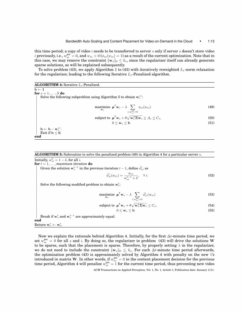
To solve problem (43), we apply Algorithm 1 to (43) with iteratively reweighted L1-norm relaxationfor the regularizer, leading to the following Iterative L1-Penalized algorithm.
ALGORITHM 4: Iterative L1-Penalized.b← 1for s = 1, . . . , S do
Solve the following subproblem using Algorithm 5 to obtain w∗∗s :
maximizews
µµµTws − λ∑
i:wpresi =0
φsi(wsi) (49)
subject to µµµTws + θ√
wTs Σws ≤ As ≤ Cs, (50)
0 ≤ ws ≤ b (51)
b← b−w∗∗s .Exit if b ≤ 0.
end
ALGORITHM 5: Subroutine to solve the penalized problem (49) in Algorithm 4 for a particular server s.Initially, w0
si = 1− δ, for all i.for t = 1, . . . ,maximum iteration do
Given the solution wt−1s in the previous iteration t− 1, define φt
si as
φtsi(wsi) =
wsi
wt−1si + δ
, ∀ i. (52)
Solve the following modified problem to obtain wts:
maximizews
µµµTws − λ∑
i:wpresi =0
φtsi(wsi) (53)
subject to µµµTws + θ√
wTs Σws ≤ Cs, (54)
0 ≤ ws ≤ b (55)
Break if wts and wt−1
s are approximately equal.endReturn w∗s ← wt
s.
Now we explain the rationale behind Algorithm 4. Initially, for the first ∆t-minute time period, weset wpre
si = 0 for all s and i. By doing so, the regularizer in problem (43) will drive the solutions Wto be sparse, such that the placement is sparse. Therefore, by properly setting λ in the regularizer,we do not need to include the constraint ‖ws‖0 ≤ ks. For each ∆t-minute time period afterwards,the optimization problem (43) is approximately solved by Algorithm 4 with penalty on the new 1’sintroduced in matrix W. In other words, if wpre
si = 0 in the content placement decision for the previoustime period, Algorithm 4 will penalize wpre
si = 1 for the current time period, thus preventing new videoACM Transactions on Applied Perception, Vol. 1, No. 1, Article 1, Publication date: January 1111.

1:14 • D. Niu, H. Xu and B. Li
copies from being created or transferred. Since the content placement for the first time period is sparseand each subsequent period penalizes the difference from the previous period, the content placementsfor subsequent periods also tend to be sparse. This fact will be demonstrated in Sec. 6 through trace-driven simulations.
5. DEMAND PREDICTION
The derivation of load direction decisions critically depends on parameters uuu and Σ, which are esti-mates of the expected demands and demand covariances for the short-term future [t, t + ∆t). In thissection, we present efficient time series forecasting methods to make such predictions based on pastobservations.
We assume that the bandwidth demand of channel i at any point in the period [t, t + ∆t) can berepresented by the same random variable Dit. This is a reasonable assumption when ∆t is small.Similarly, let µµµt = [µ1t, . . . , µNt] and Σt = [σijt] represent the demand expectation vector and demandcovariance matrix for all N channels in [t, t+∆t). We assume that before time t, the system has alreadycollected enough demand history from cloud monitoring services with a sampling interval of ∆t. Thequestion is how to use the available sampled bandwidth demand history {Diτ : τ = 0, . . . , t − 1, i =1, . . . , N} to estimate µµµt and Σt?
In this paper, we combine our previously proposed seasonal ARIMA model [Niu et al. 2011b] for con-ditional mean (expectation conditioned on the history) prediction with the GARCH model [Niu et al.2011a] for conditional variance prediction to obtain a multivariate GARCH model that can forecastthe demand covariance matrix. The model extracts the periodic evolution pattern from each channel’sdemand time series, and characterizes the remaining innovation series as autocorrelated GARCH pro-cesses. We briefly describe these statistical models here.
The difficulty in modeling the bandwidth demand of a channel i is that it exhibits diurnal periodicity,a downward trend as the video becomes less popular over time, and changing levels of fluctuationas population goes up and down. Such non-stationarity in traffic renders unbiased linear predictorsuseless. We tackle this problem by applying one-day-lagged differences (the lag is 144 if ∆t = 10minutes) onto {Diτ} to remove daily periodicity to obtain the transformed series {D′iτ := Diτ−Diτ−144},which can be modeled as a low-order autoregressive moving-average (ARMA) process:{
D′iτ − φiD′iτ−1 = Niτ + γiNiτ−1,D′iτ = Diτ −Di,τ−144,
(56)
where {Niτ} ∼WN(0, σ2) denotes the uncorrelated white noise with zero mean. Model (56) falls in thecategory of seasonal ARIMA models [Niu et al. 2011b], [Box et al. 2008].
Model parameters φi and γi in (56) can be trained based on historical data using a maximum like-lihood estimator [Box et al. 2008]. To predict the expected demand µit of channel i, we first predictµ′it := E[D′it|D′it−1, D′it−2, . . .] for the transformed series {D′iτ} to obtain the estimate µ′it, using an un-biased minimum mean square error (MMSE) predictor. We then retransform µ′it into an estimate µit ofthe conditional mean µit, with the inverse of one-day-lagged differencing.
Given the conditional means {µiτ} of channel i over all time τ , we denote the innovations in {Diτ}by {Ziτ}, where
Ziτ := Diτ − µiτ . (57)
Since the innovation term Ziτ represents the fluctuation of Diτ relative to its projected expectationµiτ , and such fluctuation may be changing over time, we model the innovations {Ziτ} using a GARCHACM Transactions on Applied Perception, Vol. 1, No. 1, Article 1, Publication date: January 1111.

Bandwidth Auto-Scaling and Content Placement for Video-on-Demand in the Cloud • 1:15
process: {Ziτ =
√hiτeτ , {eτ} ∼ IIDN (0, 1),
hiτ = αi0 + αi1Z2iτ−1 + βihiτ−1,
(58)
where {Ziτ} is modeled as a zero-mean Gaussian process yet with a time-varying conditional variancehiτ . Instead of assuming a constant variance for {Ziτ}, (58) introduces autocorrelation into volatilityevolution and forecasts the conditional variance hit of Zit as a regression of past hiτ and Z2
iτ . The modelparameters in (58) can be learned using maximum likelihood estimation (pp. 417, [Box et al. 2008])based on training data.
Furthermore, the instantaneous shocks to demands for different videos can be correlated in a large-scale system. An increase in one video’s demand may or may not affect the demand for other videosdepending on factors like video genres, release time, etc. To incorporate demand correlation, instead ofestimating volatility for each video separately, we can estimate the time-varying conditional covariancematrix Σt using multivariate GARCH [Enders 2010]. However, multivariate GARCH models are verydifficult to estimate for large-scale problems. For the 2-video case, the number of model parameters toestimate in GARCH(1, 1) is 21, and for the 3-video case, such a number escalates to 78.
To efficiently predict the covariance matrix Σt, we introduce a constant conditional correlation (CCC)model [Enders 2010], which is a popular multivariate GARCH specification that restricts the correla-tion coefficients ρij to be constant. ρij can be estimated as the correlation coefficient between series{Ziτ} and {Zjτ} in recent time periods, and ρij = 1 if i = j. The covariance σijt between video i and jat time t is thus predicted as
σijt = hijt = ρij√hithjt, (59)
with hit and hjt predicted using (58) for channels i and j individually.The full statistical model is a seasonal ARIMA conditional mean model (56) with a CCC multivariate
GARCH innovation model given by (58) and (59). The above seemingly complex model is extremelyefficient to train, as the five parameters φi, γi, αi0, αi1 and βi are learned for each video i separatelyfollowing the procedures mentioned above, and ρij is calculated straightforwardly from recent history.
5.1 Model Validation via Real Traces
We verify the effectiveness of the proposed workload prediction models based on the workload traces ofUUSee video-on-demand system over a 21-day period during 2008 Summer Olympics [Liu et al. 2010].As a commercial VoD company, UUSee streams on-demand videos to millions of Internet users acrossover 40 countries through a downloadable client software. The dataset collected contains performancesnapshots taken at a 10-minute frequency of 1693 video channels, including sports events, movies, TVepisodes and other genres. The statistics we use in this paper are the time-averaged total bandwidthdemand in each video channel in each 10-minute period. There are 144 time periods in a day.
As an example, we make 10-minute-ahead (one-step) prediction of the bandwidth demand of a pop-ular video channel i = 121 released at time period t0 = 264 (2008-08-10 10:47:39). The channel hasa maximum online population of 2664. The bandwidth consumption series of the first 1.25 days isused as the training data starting from time period 81. The initial 80 time periods are excluded whichmay not conform to later evolution patterns. The prediction is tested on the data of 3 days followingthe training period. We fit the low-order models (56) and (58) to the training data and obtain modelparameters through a maximum likelihood estimator [Box et al. 2008]. As shown in Fig. 4, such alow-order model merely trained based on the data of 1.25 days can yield conditional mean predictionsthat are close to the actual demand. The resulted prediction errors plotted in Fig. 4(b), with a mean ofzero, have a varying conditional standard deviation predicted by the GARCH model in Fig. 4(c).
ACM Transactions on Applied Perception, Vol. 1, No. 1, Article 1, Publication date: January 1111.

1:16 • D. Niu, H. Xu and B. Li
344 416 488 525 597 669 741 813 8850
100
200
300
400
500
600
700
800
900
Time (unit: 10 minutes)
Aggr
egat
e ba
ndw
idth
(Mbp
s)
Trace data1 step predictionTraining data
(a) One-step conditional mean demand prediction
525 597 669 741 813 88515010050
050
100150
Time (unit: 10 minutes)
Erro
rs (M
bps)
(b) Prediction errors
525 597 669 741 813 88535
40
45
50
55
Time (unit: 10 minutes)
Stan
dard
dev
iatio
n (M
bps)
(c) One-step prediction for conditional standard deviation
Fig. 4: 10-minute-ahead (one-step) prediction for the bandwidth demand of a popular video channel i = 121.
Then, we verify that Dit approximately follows a Gaussian distribution in each 10-minute period.Recall that for each channel i, given conditional mean prediction µit at time t, the innovation is Zit :=Dit− µit. Fig. 5(a) shows the QQ plot of Zit for a typical channel i = 121, which indicates {Zit} sampledat 10-minute intervals is a Gaussian process. Thus, it is reasonable to assume Dit follows a Gaussiandistribution within the 10 minutes following t, with mean µit. Fig. 5(b) shows the QQ plot of
∑i Zit,
which indicates that the aggregated demand∑iDit tends to Gaussian even if Djt is not for some
channel j. Since the load Ls of each server is aggregated from many videos, it is reasonable to assumeLs is Gaussian.ACM Transactions on Applied Perception, Vol. 1, No. 1, Article 1, Publication date: January 1111.

Bandwidth Auto-Scaling and Content Placement for Video-on-Demand in the Cloud • 1:17
3 2 1 0 1 2 315
10
5
0
5
10
15
Standard Normal Quantiles
Qua
ntile
s of
Inpu
t Sam
ple
(a) Zit of a typical channel
3 2 1 0 1 2 31500
1000
500
0
500
1000
1500
Standard Normal Quantiles
Qua
ntile
s of
Inpu
t Sam
ple
(b)∑
i Zit of all channels combined
Fig. 5: QQ plot of innovations for t =1562—1640 vs. normal distribution.
0
100
200
300
400
Aggr
egat
e ba
ndw
idth
(Mbp
s)
Day 12 Day 13 Day 14Day 10 Day 11 Day 12
Video959F2Video4E0B2
0
100
200
300
400
Aggr
egat
e ba
ndw
idth
(Mbp
s)
Day 16 Day 17 Day 18Day 10 Day 11 Day 12
Video9AB4AVideo4E50A
Fig. 6: Videos released on different days but at the same time of day exhibit similar initial demand patterns.
5.2 A Channel Interleaving Scheme
Although we have presented a complete framework for efficient forecasts of expected future demandµt and demand covariance matrix Σt, the parameter learning for the seasonal ARIMA model (56)requires a training data of more than 1 day (specifically 1.25 days in our predictor) to incorporatedaily periodicity into the model. As new videos do not have enough historical observations for modeltraining, their demands can hardly be forecasted from history. In this section, we propose methods topredict demands for newly released videos that lack historical observations and unpopular small videochannels. We tackle this issue by intelligently interleaving traffic of new videos to form “virtualizedvideo channels” for demand prediction. We also use a similar technique to combine small channels toimprove prediction accuracy.
Let us consider new videos that have been in the system for less than 1.25 days. Although thesevideos do not have sufficient historical observations for model training, we observe that their initialdemand patterns are quite similar to videos that were released earlier around the same time of day.For example, the left half of Fig. 6 shows the initial demands of 2 video channels 959F2 and 4E0B2
ACM Transactions on Applied Perception, Vol. 1, No. 1, Article 1, Publication date: January 1111.

1:18 • D. Niu, H. Xu and B. Li
released at 2008-08-19 21:31:56 and 2008-08-17 21:23:20, respectively. As both videos are releasedaround the same time of day, though on different days, they are aligned in Fig. 6 for comparison, withdouble lines of x-labels showing the first 3 days of each video. (2008-08-08 is deemed as Day 1 andthe first time period of each day is 14:50.) We can see the two videos exhibit a similar initial demandevolution pattern, though with different popularity. The major reason for such similarity is that mostusers watch VoD channels around several peak times in a day: both videos are released between 21:00and 22:00 and will expect the first peak demand at midnight, followed by a second peak at noon onthe next day. Similarly, the right half of Fig. 6 compares the initial demands of video 9AB4A releasedat 2008-08-23 17:11:54 and video 4E50A released at 2008-08-17 17:02:38. They also exhibit similarinitial demand patterns, with the first peak around 18:00, which is the start of off-work hours, beforethe second peak around midnight. Different videos, however, may attract different sizes of populationdepending on their popularity.
From the above analysis, we can predict the demand for a new video based on other videos releasedon an earlier date but at the same time of day. To implement this idea, we define virtual new chan-nel k as a combination of all video channels with an age less than 1.25 days and released in hourk ∈ {1, . . . , 24} on any date. Upon release, a new video joins virtual new channel k based on its re-lease hour k, and quits this virtual new channel when it has been in the system for 1.25 days andaccumulated enough observations for separate model training. As a result, each virtual new channel kcontains a dynamic set of video channels released in hour k yet possibly on different days. For example,Fig. 7 shows the aggregate bandwidth demand of virtual new channel 11 from time 433 to 1800, andFig. 9 shows the number of videos contained in virtual new channel 11 from time 1 to 1800. We cansee that although virtual new channel 11 represents a dynamic group of videos, its aggregate band-width demand exhibits repetition of a similar pattern because the videos in this virtual channel are allreleased in hour 11, possibly on different dates.
Similarly, we aggregate small video channels and set up 24 virtual small channels. When a videoreaches the age of 1.25 days, it quits its virtual new channel. If its demand never exceeded a threshold(e.g., 40 Mbps) in the first 1.25 days, it will join one of the virtual small channels in a round robinfashion. Otherwise, it becomes a mature channel.
Each mature or virtual channel is deemed as an entity to which predictions and optimizations areapplied. For example, we make 10-minutes-ahead prediction of bandwidth demand for virtual newchannel 11, and plot the conditional mean prediction in Fig. 7 and the conditional standard deviationprediction in Fig. 8 for a test period of 1.5 days. Satisfactory prediction performance is observed. Al-though conditional mean prediction is subject to errors, the GARCH model can predict the conditionalerror standard deviation, as shown in Fig. 8, which contributes to the risk factor (11) in the bandwidthreservation minimization. Furthermore, the combination of several real video channels into a virtualchannel suppresses random shocks, making prediction more accurate.
6. PERFORMANCE EVALUATION
We conduct a series of simulations to evaluate the performance of our auto-scaling reservation schemesfor video storage systems. The simulations are driven by the replay of the workload traces of UUSeevideo-on-demand system over a 21-day period during 2008 Summer Olympics [Liu et al. 2010]. Weask the question—what the performance would have been if UUSee had all its workload in this periodserved by cloud services through our auto-scaled bandwidth reservation system?
We conduct performance evaluation for 4 typical time spans which are near the beginning, middleand end of the 21-day duration. We implement statistical learning and demand prediction techniquespresented in Sec. 5 to forecast the expected demands µµµt and demand covariance matrix Σt every 10minutes. The model parameters are retrained daily, with training data being the bandwidth demandACM Transactions on Applied Perception, Vol. 1, No. 1, Article 1, Publication date: January 1111.

Bandwidth Auto-Scaling and Content Placement for Video-on-Demand in the Cloud • 1:19
433 577 721 865 1009 1153 1297 1441 1585 18000
200
400
600
Time (unit: 10 minutes)
Aggr
egat
e ba
ndw
idth
(Mbp
s)
Trace data 1 step prediction Training data
Fig. 7: The conditional mean prediction for St in virtual new channel 11, with a test period of 1.5 days from time 1585 to 1800.Only a part of the entire training data is plotted.
1585 1657 1729 1800150
100
50
0
50
100
Time (unit: 10 minutes)
Mbp
s
Prediction errorError standard deviation
Fig. 8: The prediction error and predicted error standarddeviation for St in virtual new channel 11.
1 433 865 1297 158518000
2
4
6
8
10
Time (unit: 10 minutes)
Num
ber o
f Vid
eos
Training PeriodTest Period
Fig. 9: The number of videos in virtual new channel 11during the entire training and test periods.
series {Diτ} in the recent 1.25 days of each channel i. Once trained, the models will be used for thenext 24 hours. Although video users may join or quit a channel unexpectedly, our prediction is stilleffective, since it deals with the aggregate demand in the channel which features diurnal patterns. Weassume that there is a pool of servers from which UUSee can reserve bandwidth. To spread the loadacross servers, we set Cs = 300 Mbps for each s. The QoS parameter θ := F−1(1 − ε) is set to θ = 2.05to confine the under-provision probability to ε = 2%.
6.1 Algorithms for Comparison
We compare our optimal load direction (14) under full replication, and Algorithm 1, Algorithm 2, Algo-rithm 3 and Algorithm 4 with sparse content placement, against the following baseline algorithms:
Reactive without Prediction. Initially, replicate each video to K randomly chosen servers, whichlimits the initial content replication degree to K. Each client requesting channel i is randomly directedto a server that has video i and idle bandwidth capacity. A request is dropped if there is no such server.In this case, the algorithm reacts by replicating video i to an additional server chosen randomly thathas idle capacity. Replicating content is not instant: we assume that the replication involves a delay ofone period of time.
ACM Transactions on Applied Perception, Vol. 1, No. 1, Article 1, Publication date: January 1111.

1:20 • D. Niu, H. Xu and B. Li
Table I. : The performance of different schemes averaged over each test period, in terms of QoS, resource utilization, andreplication.
Periods Time periods 702—780 (91 mature and virtual channels) Time periods 1422—1480 (161 mature and virtual channels)Peak demand 6.56 Gbps, mean demand 5.19 Gbps Peak demand 6.81 Gbps, mean demand 4.91 Gbps
Short Drop Util Rep Booked Over-prov Short Drop Util Rep Booked Over-provOptimal 0 Chs 0.66% 92.9% 91.0 6.57 Gbps 108.5% 0 Chs 0.25% 91.1% 161.0 6.38 Gbps 110.3%
Per-Server Opt 1.0 Chs 0.37% 90.0% 8.5 6.79 Gbps 112.2% 1.2 Chs 0.13% 88.6% 6.9 6.56 Gbps 113.4%Per-Server Lim 0.3 Chs 0.06% 85.7% 2.6 7.13 Gbps 117.8% 0.2 Chs 0.03% 84.6% 2.4 6.86 Gbps 118.8%
Random 5.9 Chs 0.02% 83.3% 3.8 7.33 Gbps 121.2% 7.6 Chs 0.00% 82.2% 3.0 7.08 Gbps 122.4%Reactive 7.9 Chs 0.47% 77.2% 4.3 7.91 Gbps 132.4% 7.2 Chs 0.34% 70.4% 3.6 8.20 Gbps 146.0%
Itr L1-Constr 0 Chs 0.18% 88.2% 4.8 6.92 Gbps 114.3% - - - - - -Itr L1-Penal 0.1 Chs 0.06% 85.1% 2.3 7.18 Gbps 118.7% 0.1 Chs 0% 84.7% 2.3 6.88 Gbps 118.8%
Periods Time periods 1562—1640 (176 mature and virtual channels) Time periods 2402—2500 (199 mature and virtual channels)Peak demand 7.55 Gbps, mean demand 5.62 Gbps Peak demand 9.19 Gbps, mean demand 7.62 Gbps
Short Drop Util Rep Booked Over-prov Short Drop Util Rep Booked Over-provOptimal 0 Chs 0.31% 91.1% 176.0 7.27 Gbps 110.4% 0 Chs 0.11% 85.4% 199.0 10.54 Gbps 118.1%
Per-Server Opt 0.7 Chs 0.16% 88.3% 7.3 7.51 Gbps 114.0% 1.0 Chs 0.09% 82.7% 6.3 10.87 Gbps 121.8%Per-Server Lim 1.4 Chs 0.00% 83.9% 2.4 7.89 Gbps 119.9% 20.7 Chs 0.17% 82.3% 2.5 10.95 Gbps 122.6%
Random 6.2 Chs 0.00% 80.4% 3.3 8.28 Gbps 125.4% 33.4 Chs 0.02% 77.9% 4.5 11.54 Gbps 129.3%Reactive 5.9 Chs 0.27% 72.7% 3.5 9.08 Gbps 140.4% 15.8 Chs 0.43% 74.6% 3.6 12.01 Gbps 140.3%
Itr L1-Penal 1.1 Chs 0.03% 84.5% 2.0 7.85 Gbps 119.1% 1.0 Chs 0.01% 81.1% 2.1 11.92 Gbps 124.5%
Short: Average # channels with dropped requests; Drop: average request drop rate; Util: average utilization of allo-cated resources; Rep: average replication degree; Booked: average booked bandwidth; Over-prov: average over-provisioningratio.Note: Iterative L1-Constrained is only evaluated for time periods 702-780, since it cannot efficiently complete within 10 minutesfor more than 91 channels, which is the case for other time spans.
Random with Prediction. Initially, let s = 1 and b = 1. Second, randomly generate ws in (0,b)and rescale it so that the QoS constraint (11) is achieved with equality for s. Update b to b −ws andupdate s to s+1. Go to the second step unless b = 0 or s = S+1, in which case the program terminates.
The reactive scheme represents provisioning for peak demand in Fig. 1 in some way, with limitedreplication. It does not leverage prediction or bandwidth reservation. We assume in Reactive, the totalcloud capacity allocated is always the minimum capacity needed to meet the peak demand in thesystem. The random scheme leverages prediction and makes bandwidth reservation, but randomlydirects workloads instead of using anti-correlation and optimization techniques to minimize bandwidthreservation.
We implement all of the six schemes discussed above, and summarize their performance comparisonin Table I for each of the four time spans. Iterative L1-Constrained is only evaluated for time periods702-780, as it cannot converge within 10 minutes for more than 91 channels. Note that the channelsin the table include mature channels, virtual new channels and virtual small channels. The numberof videos in each virtual channel can vary over time. As new videos are introduced, more channels arepresent in later test periods. We evaluate the algorithm performance with regard to QoS, bandwidthresource occupied, and replication cost.
6.2 The Benefit of Predictive Provisioning over Reactive Provisioning
Table I shows that Reactive generally has a more salient QoS problem than all five predictive schemesin terms of both the number of unsatisfied channels and request drop rate (percentage of unsatisfied re-quests), demonstrating the benefit of demand prediction. Fig. 10 presents a more detailed comparisonfor a typical peak period from time 702 to 780. Without surprise, Reactive has many unfulfilled re-quests at the beginning. Since the videos are randomly replicated to K = 2 servers (shown in Fig. 10(d)at t = 702) and requests are randomly directed, it is likely that a channel does not acquire enough ca-ACM Transactions on Applied Perception, Vol. 1, No. 1, Article 1, Publication date: January 1111.

Bandwidth Auto-Scaling and Content Placement for Video-on-Demand in the Cloud • 1:21
Time (unit: 10 minutes)702 712 722 732 742 752 762 772 780
Un
se
rve
d d
em
an
d (
%)
0
2
4
6
8
10
12Per-server optimizationPer-server limited channelsIterative L1-constrainedReactive without prediction
(a) Request drop rate (% unsatisfied requests)
Time (unit: 10 minutes)702 712 722 732 742 752 762 772 780
Un
sa
tisfie
d c
ha
nn
els
0
10
20
30
40
50Per-server optimizationPer-server limited channelsIterative L1-constrainedReactive without prediction
(b) Number of channels with unsatisfied requests
Time (unit: 10 minutes)702 712 722 732 742 752 762 772 780
Utiliz
atio
n (
%)
40
50
60
70
80
90
100
110
Per-server optimizationPer-server limited channelsIterative L1-constrainedReactive without prediction
(c) Utilization of reserved resource
Time (unit: 10 minutes)702 712 722 732 742 752 762 772 780
Re
plic
atio
n d
eg
ree
0
5
10
15
20
25
30
35Per-server optimizationPer-server limited channelsIterative L1-constrainedReactive without prediction
(d) Replication degree
Fig. 10: Predictive vs. reactive bandwidth provisioning for a typical peak period 702–780. There are35 servers available, each with capacity 300 Mbps, and 91 channels, including 52 popular channels,24 small channels, 15 non-zero new channels. For Reactive, K = 2. For Iterative L1-Constrained, thenumber of videos per server is ks = 5 for all s. For all other schemes, ks = 10 for all s.
pacity to meet its demand. As Reactive detects the QoS problem, videos are replicated to more serversto acquire more capacity, with a gradually increased replication degree over time, as in Fig. 10(d). Wecan see that after 140 minutes, when the replication degree exceeds 4, the QoS of Reactive becomesrelatively stable in Fig. 10(a). However, around time 763, Reactive suffers from salient QoS problemsagain, due to a sudden ramp-up of demand. In contrast, the predictive schemes foresee and get pre-pared for demand changes, resulting in much better QoS, even in the event of drastic demand increase.
The predictive schemes also achieve higher resource utilization. Utilization of a predictive scheme isthe ratio between the actual bandwidth usage and the total booked bandwidth in all servers. For Reac-tive, the utilization is the actual bandwidth demand divided by the peak demand. Although Fig. 10(c)shows that Reactive achieves a high utilization for the peak demand around time 763, its averageutilization is merely 77.19% in the test period from 702 to 780. Predictive auto-scaling enhances uti-lization to 85.7% with Per-Server Limited Channels, to 90.0% with Per-Server Optimal, to 88.2% withIterative L1-Constrained and to 92.9% with the theoretical optimal solution under full replication.
ACM Transactions on Applied Perception, Vol. 1, No. 1, Article 1, Publication date: January 1111.

1:22 • D. Niu, H. Xu and B. Li
Time (unit: 10 minutes)702 712 722 732 742 752 762 772 780
Mb
ps
-1000
0
1000
2000
3000 Per-server optimizationPer-server limited channelsIterative L1-penalizedRandom
(a) Cushion bandwidth (reserved - used)
Time (unit: 10 minutes)702 712 722 732 742 752 762 772 780
Imp
rove
me
nt
(%)
-20
0
20
40
60
80
100
120Per-server optimization vs. RandomPer-server limited channels vs. RandomIterative L1-penalized vs. Random
(b) Savings on cushion bandwidth (702—780)
Time (unit: 10 minutes)1422 1432 1442 1452 1462 1472 1480
Mb
ps
-500
0
500
1000
1500
2000
2500
3000Per-server optimizationPer-server limited channelsIterative L1-penalizedRandom
(c) Cushion bandwidth (reserved - used)
Time (unit: 10 minutes)1422 1432 1442 1452 1462 1472 1480
Imp
rove
me
nt
(%)
0
20
40
60
80
100Per-server optimization vs. RandomPer-server limited channels vs. RandomIterative L1-penalized vs. Random
(d) Savings on cushion bandwidth (1422—1480)
Time (unit: 10 minutes)1562 1572 1582 1592 1602 1612 1622 1632 1640
Mb
ps
0
1000
2000
3000Per-server optimizationPer-server limited channelsIterative L1-penalizedRandom
(e) Cushion bandwidth (reserved - used)
Time (unit: 10 minutes)1562 1572 1582 1592 1602 1612 1622 1632 1640
Imp
rove
me
nt
(%)
0
20
40
60
80
100
120Per-server optimization vs. RandomPer-server limited channels vs. RandomIterative L1-penalized vs. Random
(f) Savings on cushion bandwidth (1562—1640)
Time (unit: 10 minutes)2402 2412 2422 2432 2442 2452 2462 2472 2480
Mb
ps
-2000
0
2000
4000
6000
8000Per-server optimizationPer-server limited channelsIterative L1-penalizedRandom
(g) Cushion bandwidth (reserved - used)
Time (unit: 10 minutes)2402 2412 2422 2432 2442 2452 2462 2472 2480
Imp
rove
me
nt
(%)
-40
-20
0
20
40
60
80
Per-server optimization vs. RandomPer-server limited channels vs. RandomIterative L1-penalized vs. Random
(h) Savings on cushion bandwidth (2402—2480)
Fig. 11: Workload portfolio selection vs. random load direction for different time periods. For all theschemes, the number of videos per server is ks = 10 for all s.
6.3 Resource Autoscaling: a Comparison among Predictive Schemes
We now compare the six predictive schemes. Among them, as shown in Table I, Optimal books theminimum necessary bandwidth and achieves the highest bandwidth utilization, yet with the highestACM Transactions on Applied Perception, Vol. 1, No. 1, Article 1, Publication date: January 1111.

Bandwidth Auto-Scaling and Content Placement for Video-on-Demand in the Cloud • 1:23
Time (unit: 10 minutes)702 712 722 732 742 752 762 772 780
# S
erv
ers
Use
d
15
20
25
30
35
Per-server optimizationPer-server limited channelsIterative L1-penalizedRandom
(a) Server autoscaling for time periods 702–780
Time (unit: 10 minutes)1422 1432 1442 1452 1462 1472 1481
# S
erv
ers
Use
d
15
20
25
30
35
40Per-server optimizationPer-server limited channelsIterative L1-penalizedRandom
(b) Server autoscaling for time periods 1422–1480
Time (unit: 10 minutes)1562 1572 1582 1592 1602 1612 1622 1632 1640
# S
erv
ers
Use
d
15
20
25
30
35
40Per-server optimizationPer-server limited channelsIterative L1-penalizedRandom
(c) Server autoscaling for time periods 1562–1640
Time (unit: 10 minutes)2402 2412 2422 2432 2442 2452 2462 2472 2480
# S
erv
ers
Use
d
20
25
30
35
40
45
50
Per-server optimizationPer-server limited channelsIterative L1-penalizedRandom
(d) Server autoscaling for time periods 2402–2500
Fig. 12: Server autoscaling: the number of servers used by each predictive provisioning scheme in eachtime period for 4 different time spans.
replication overhead. In fact, with full replication, each video is replicated to every server, and thusthe optimal solution can best exploit the anti-correlations among all the channels to minimize reservedbandwidth. However, the VoD provider needs to pay a high storage cost to the cloud service provider.
Among all the five predictive schemes that replicate content sparsely, Random achieves the lowestutilization, since it is completely blind to the correlation information in workload selection and di-rection. Per-Server Optimal can reduce the replication degree while maintaining other performancemetrics. By further imposing a channel number constraint on each server, Per-Server Limited Chan-nels strikes a balance between replication overhead and bandwidth utilization. It aggressively reducesthe replication degree to a very small value of 2.4-2.6 copies per video. Iterative L1-penalized turns outto be a numerically stable method which yields the smallest replication degree among all the predictiveschemes, with an extremely low drop rate and an over-provisioning ratio that is only slightly higherthan Optimal and comparable to Per-Server Limited Channels.
Nonetheless, Iterative L1-Constrained, as shown in Fig. 10(c) and Fig. 10(d), achieves a slightlyhigher utilization of booked bandwidth than Per-Server Limited Channels at the cost of a higher repli-cation degree. The request drop rates and numbers of unsatisfied channels in both schemes are similarto each other, as shown in Fig. 10(a) and Fig. 10(b). Note that for Iterative L1-Constrained, we haveset the number of videos per server to be ks = 5, which is one half of that in other schemes. The reasonis that in Iterative L1-Constrained, the modified constraint
∑i φ
tsi(wsi) ≤ ks does not always converge
to the video number (L0-norm) constraint per server ‖ws‖0 ≤ ks. In Fig. 10(d), the spikes in the repli-cation degree corresponds to the time periods where the iterative program aborts in an iteration whenthere is no feasible solution to constraints (39)-(42). In such cases, the modified constraint (42), i.e.,∑i φ
tsi(wsi) ≤ ks never converges to ‖ws‖0 ≤ ks. Thus, there exist much higher replication degrees in
such time periods, although ks is set to a low value. In fact, it is challenging to tune the parameter δ soACM Transactions on Applied Perception, Vol. 1, No. 1, Article 1, Publication date: January 1111.
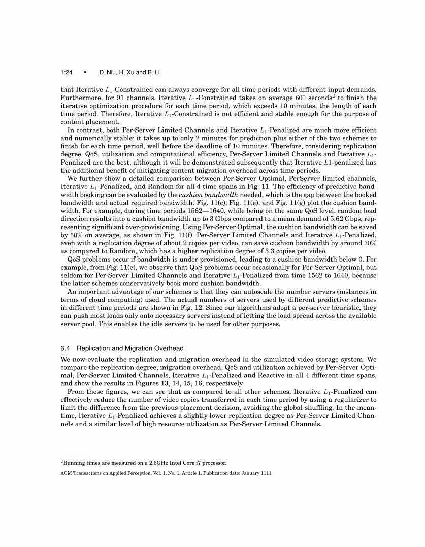
1:24 • D. Niu, H. Xu and B. Li
that Iterative L1-Constrained can always converge for all time periods with different input demands.Furthermore, for 91 channels, Iterative L1-Constrained takes on average 600 seconds2 to finish theiterative optimization procedure for each time period, which exceeds 10 minutes, the length of eachtime period. Therefore, Iterative L1-Constrained is not efficient and stable enough for the purpose ofcontent placement.
In contrast, both Per-Server Limited Channels and Iterative L1-Penalized are much more efficientand numerically stable: it takes up to only 2 minutes for prediction plus either of the two schemes tofinish for each time period, well before the deadline of 10 minutes. Therefore, considering replicationdegree, QoS, utilization and computational efficiency, Per-Server Limited Channels and Iterative L1-Penalized are the best, although it will be demonstrated subsequently that Iterative L1-penalized hasthe additional benefit of mitigating content migration overhead across time periods.
We further show a detailed comparison between Per-Server Optimal, PerServer limited channels,Iterative L1-Penalized, and Random for all 4 time spans in Fig. 11. The efficiency of predictive band-width booking can be evaluated by the cushion bandwidth needed, which is the gap between the bookedbandwidth and actual required bandwidth. Fig. 11(c), Fig. 11(e), and Fig. 11(g) plot the cushion band-width. For example, during time periods 1562—1640, while being on the same QoS level, random loaddirection results into a cushion bandwidth up to 3 Gbps compared to a mean demand of 5.62 Gbps, rep-resenting significant over-provisioning. Using Per-Server Optimal, the cushion bandwidth can be savedby 50% on average, as shown in Fig. 11(f). Per-Server Limited Channels and Iterative L1-Penalized,even with a replication degree of about 2 copies per video, can save cushion bandwidth by around 30%as compared to Random, which has a higher replication degree of 3.3 copies per video.
QoS problems occur if bandwidth is under-provisioned, leading to a cushion bandwidth below 0. Forexample, from Fig. 11(e), we observe that QoS problems occur occasionally for Per-Server Optimal, butseldom for Per-Server Limited Channels and Iterative L1-Penalized from time 1562 to 1640, becausethe latter schemes conservatively book more cushion bandwidth.
An important advantage of our schemes is that they can autoscale the number servers (instances interms of cloud computing) used. The actual numbers of servers used by different predictive schemesin different time periods are shown in Fig. 12. Since our algorithms adopt a per-server heuristic, theycan push most loads only onto necessary servers instead of letting the load spread across the availableserver pool. This enables the idle servers to be used for other purposes.
6.4 Replication and Migration Overhead
We now evaluate the replication and migration overhead in the simulated video storage system. Wecompare the replication degree, migration overhead, QoS and utilization achieved by Per-Server Opti-mal, Per-Server Limited Channels, Iterative L1-Penalized and Reactive in all 4 different time spans,and show the results in Figures 13, 14, 15, 16, respectively.
From these figures, we can see that as compared to all other schemes, Iterative L1-Penalized caneffectively reduce the number of video copies transferred in each time period by using a regularizer tolimit the difference from the previous placement decision, avoiding the global shuffling. In the mean-time, Iterative L1-Penalized achieves a slightly lower replication degree as Per-Server Limited Chan-nels and a similar level of high resource utilization as Per-Server Limited Channels.
2Running times are measured on a 2.6GHz Intel Core i7 processor.
ACM Transactions on Applied Perception, Vol. 1, No. 1, Article 1, Publication date: January 1111.

Bandwidth Auto-Scaling and Content Placement for Video-on-Demand in the Cloud • 1:25
Time (unit: 10 minutes)702 712 722 732 742 752 762 772 780
Un
se
rve
d d
em
an
d (
%)
0
2
4
6
8
10
12Per-server optimizationPer-server limited channelsIterative L1-penalizedReactive without prediction
(a) Request drop rate (% unsatisfied requests)
Time (unit: 10 minutes)702 712 722 732 742 752 762 772 780
Utiliz
atio
n (
%)
40
50
60
70
80
90
100
110
Per-server optimizationPer-server limited channelsIterative L1-penalizedReactive without prediction
(b) Utilization of reserved resource
Time (unit: 10 minutes)702 712 722 732 742 752 762 772 780
Re
plic
atio
n d
eg
ree
0
5
10
15
20
25
30
35Per-server optimizationPer-server limited channelsIterative L1-penalizedReactive without prediction
(c) Replication degree
Time (unit: 10 minutes)702 712 722 732 742 752 762 772 780
# V
ide
os M
igra
ted
0
50
100
150
200
250
300Per-server optimizationPer-server limited channelsIterative L1-penalizedReactive without prediction
(d) Number of video copies migrated
Fig. 13: Performance of different schemes for a typical peak period 702–780. There are 35 serversavailable, each with capacity 300 Mbps, and 91 mature and virtual channels. For Reactive, K = 2. ForPer-Server Limited Channels, ks = 10 for all s.
Furthermore, the execution of Iterative L1-Penalized is quite light-weight in our simulation. In thesubroutine, Algorithm 5, we set maxiteration = 5, and set λ(1) = 0 and
λ(t) =1
5· µµµTwt−1
s∑i:wpre
si=0 φtsi(w
t−1si )
, t = 2, 3, 4, 5.
With the above setting, it takes less than 1 minute to execute Iterative L1-Penalized and the solutionis already sparse enough.
7. RELATED WORK
Researches on exploiting virtualization techniques for delivering cloud-based IPTV services have beenconducted by major VoD providers like AT&T [Aggarwal et al. 2011]. The importance of VoD bandwidthdemand prediction to capacity planning has also been recognized. It is shown that demand estimatescan help with optimal content placement in AT&T’s IPTV network [Applegate et al. 2010].
ACM Transactions on Applied Perception, Vol. 1, No. 1, Article 1, Publication date: January 1111.

1:26 • D. Niu, H. Xu and B. Li
Time (unit: 10 minutes)1422 1432 1442 1452 1462 1472 1480
Un
se
rve
d d
em
an
d (
%)
0
2
4
6
8
10
12Per-server optimizationPer-server limited channelsIterative L1-penalizedReactive without prediction
(a) Request drop rate (% unsatisfied requests)
Time (unit: 10 minutes)1422 1432 1442 1452 1462 1472 1480
Utiliz
atio
n (
%)
50
60
70
80
90
100
110
Per-server optimizationPer-server limited channelsIterative L1-penalizedReactive without prediction
(b) Utilization of reserved resource
Time (unit: 10 minutes)1422 1432 1442 1452 1462 1472 1480
Re
plic
atio
n d
eg
ree
0
5
10
15
20
25
30
35Per-server optimizationPer-server limited channelsIterative L1-penalizedReactive without prediction
(c) Replication degree
Time (unit: 10 minutes)1422 1432 1442 1452 1462 1472 1480
# V
ide
os M
igra
ted
0
50
100
150
200
250
300
350
400Per-server optimizationPer-server limited channelsIterative L1-penalizedReactive without prediction
(d) Number of video copies migrated
Fig. 14: Performance of different schemes for a typical peak period 1422–1480. There are 36 serversavailable, each with capacity 300 Mbps, and 161 mature and virtual channels. For Reactive, K = 2. ForPer-Server Limited Channels, ks = 10 for all s.
The traffic characteristics of the two popular video streaming services, Netflix and YouTube, arestudied in [Rao et al. 2011], where it is observed that the bandwidth of links carrying video streamingtraffic should be provisioned to E[R(t)] + α
√Var[R(t)], where R(t) is the aggregate data rate of the
video streaming traffic at time t. α ≥ 1 is a constraint on the tolerable bandwidth violations. Furthermore, it is pointed out in [Rao et al. 2011] that the mean and variance of the aggregate data rate ofvideo streaming traffic are independent of the underlying streaming strategies used, which may rangefrom non-ack clocked ON-OFF cycles to bulk TCP transfer, depending on the type of the application(Web browser or native mobile application) and the type of container (Silverlight, Flash, or HTML5)used. Hence, the required bandwidth is also independent of these diverse factors. This implies thatvideo services can safely select a streaming strategy that can be optimized for other goals such asserver load without overwhelming the network.
Due to the predictability of aggregate video traffic, several time-series and statistical learning meth-ods have been applied to video traffic prediction, including non-stationary time series models [Niuet al. 2011b], [Niu et al. 2011a], and video access pattern extraction via principal component analysis[Gursun et al. 2011].ACM Transactions on Applied Perception, Vol. 1, No. 1, Article 1, Publication date: January 1111.

Bandwidth Auto-Scaling and Content Placement for Video-on-Demand in the Cloud • 1:27
Time (unit: 10 minutes)1562 1572 1582 1592 1602 1612 1622 1632 1640
Un
se
rve
d d
em
an
d (
%)
0
2
4
6
8
10
12Per-server optimizationPer-server limited channelsIterative L1-penalizedReactive without prediction
(a) Request drop rate (% unsatisfied requests)
Time (unit: 10 minutes)1562 1572 1582 1592 1602 1612 1622 1632 1640
Utiliz
atio
n (
%)
40
50
60
70
80
90
100
110
Per-server optimizationPer-server limited channelsIterative L1-penalizedReactive without prediction
(b) Utilization of reserved resource
Time (unit: 10 minutes)1562 1572 1582 1592 1602 1612 1622 1632 1640
Re
plic
atio
n d
eg
ree
0
5
10
15
20
25
30
35Per-server optimizationPer-server limited channelsIterative L1-penalizedReactive without prediction
(c) Replication degree
Time (unit: 10 minutes)1562 1572 1582 1592 1602 1612 1622 1632 1640
# V
ide
os M
igra
ted
0
100
200
300
400
500Per-server optimizationPer-server limited channelsIterative L1-penalizedReactive without prediction
(d) Number of video copies migrated
Fig. 15: Performance of different schemes for a typical peak period 1562–1640. There are 40 serversavailable, each with capacity 300 Mbps, and 176 mature and virtual channels. For Reactive, K = 2. ForPer-Server Limited Channels, ks = 10 for all s.
Predictive and dynamic resource provisioning has been proposed mostly for virtual machines (VM)and web applications with respect to CPU utilization [Bobroff et al. 2007], [Gong et al. 2010], [Tanget al. 2007], [Gmach et al. 2007] and power consumption [Kusic et al. 2009], [Lin et al. 2011]. VMconsolidation with dynamic bandwidth demand has also been considered in [Wang et al. 2011]. Ourwork exploits the unique characteristics of VoD bandwidth demands and distinguishes from the abovework in three aspects. First, our bandwidth workload consolidation is as simple as solving convexoptimization for a load direction matrix. We leverage the fact that unlike VM, demand of a VoD channelcan be fractionally split into video requests. Second, our system forecasts not only the expected demandbut also the demand volatility, and thus can control the risk factors more accurately. In contrast, mostprevious works [Gong et al. 2010], [Gmach et al. 2007] assume a constant demand variance. Third,we exploit the statistical correlation between bandwidth demands of different video channels to saveresource reservation while previous works such as [Wang et al. 2011] consider independent workloads.
The idea of statistical multiplexing and resource overbooking has been empirically evaluated fora shared hosting platform in [Urgaonkar et al. 2002]. Our novelty is that we formulate the quality-assured resource minimization problem using Value at Risk (VaR), a useful risk measure in financial
ACM Transactions on Applied Perception, Vol. 1, No. 1, Article 1, Publication date: January 1111.

1:28 • D. Niu, H. Xu and B. Li
Time (unit: 10 minutes)2402 2412 2422 2432 2442 2452 2462 2472 2480
Un
se
rve
d d
em
an
d (
%)
0
5
10
15
20Per-server optimizationPer-server limited channelsIterative L1-penalizedReactive without prediction
(a) Request drop rate (% unsatisfied requests)
Time (unit: 10 minutes)2402 2412 2422 2432 2442 2452 2462 2472 2480
Utiliz
atio
n (
%)
50
60
70
80
90
100
110
120
Per-server optimizationPer-server limited channelsIterative L1-penalizedReactive without prediction
(b) Utilization of reserved resource
Time (unit: 10 minutes)2402 2412 2422 2432 2442 2452 2462 2472 2480
Re
plic
atio
n d
eg
ree
0
5
10
15
20
25
30
35Per-server optimizationPer-server limited channelsIterative L1-penalizedReactive without prediction
(c) Replication degree
Time (unit: 10 minutes)2402 2412 2422 2432 2442 2452 2462 2472 2480
# V
ide
os M
igra
ted
0
200
400
600
800
1000
Per-server optimizationPer-server limited channelsIterative L1-penalizedReactive without prediction
(d) Number of video copies migrated
Fig. 16: Performance of different schemes for a typical peak period 2402–2480. There are 48 serversavailable, each with capacity 300 Mbps, and 199 mature and virtual channels. For Reactive, K = 2. ForPer-Server Limited Channels, ks = 10 for all s.
asset management [McNeil et al. 2005], with the aid of accurate demand correlation forecasts. Webelieve our theoretically grounded approach bears stronger robustness against intractable demandvolatility in practice.
There are extensive studies around the content placement problem in replication-based cloud storagesystems. In [Rochman et al. 2013], Rochman et al. propose the strategies of placing the resourcesto distributed datacenters to serve more requests locally. In [Xu and Li 2013], Xu et al. propose arequest mapping and response routing scheme to maximize the total utility of serving requests minusthe cost. Bonvin et al. [Bonvin et al. 2010] propose a distributed scheme to dynamically allocate theresources of a data storage cloud based on net benefit maximization, considering the utility offered bythe partition and its storage and maintenance cost. In [Agarwal et al. 2010], automatic data placementacross geo-distributed datacenters is presented, which iteratively moves a data item closer to bothclients and other data items that it communicates with. B. Yang et al. [Yu and Pan 2015] study thecontent placement problem for systems when multiple items are needed in each request and the itemsize is small. They try to maximize the correlation of the items collocated on the same server to reducethe I/O and CPU overhead to satisfy each request. In this paper, we consider video storage and accessACM Transactions on Applied Perception, Vol. 1, No. 1, Article 1, Publication date: January 1111.

Bandwidth Auto-Scaling and Content Placement for Video-on-Demand in the Cloud • 1:29
systems, where the most important performance metrics are bandwidth and storage. And we focus ongeographically collocated server clusters in a same datacenter.
Our prior work [Niu et al. 2012] has studied the optimal load direction and cloud bandwidth reser-vation under full content replication, this paper provides a deeper study on this problem in a widerscope. Specifically, in this paper, we further discuss load direction under a given sparse replicationscheme and study the joint optimization of load direction and sparse content placement in Sec. 4. Weintroduce a new algorithm to solve this joint load direction and placement problem involving L0 normsthrough iteratively reweighed L1-norm relaxations, and compare its performance with other proposedalgorithms. Furthermore, we elaborate our demand prediction schemes in Sec. 5, with detailed per-formance evaluations, and add detailed discussions on handling new channels and forming virtualchannels for improved demand prediction.
To the best of our knowledge, this is the first work that jointly models the load direction and sparsecontent placement as a sparsity-penalized or sparsity-constrained optimization problem. And we havenovelly adapted the iterative reweighted L1-norm approximation techniques from the sparse recoverytheory to solve our sparse design problem, yielding satisfactory performance and low computationalcomplexity.
8. CONCLUDING REMARKS
In this paper, we propose an unobtrusive, predictive, and elastic cloud resource auto-scaling frameworkfor video storage systems. Operated at a 10-minute frequency, the system automatically predicts theexpected future demand as well as demand volatility for each video through ARIMA and GARCHtime-series forecasting techniques based on history. Leveraging demand prediction, the system jointlymakes load direction to multiple cloud servers and make bandwidth reservations from them to satisfythe projected demands with high probability. The system can save resource reservation cost for VoDproviders in terms of both bandwidth and storage.
We exploit the predictable anti-correlation between video requests to enhance resource utilization,and derive the optimal load direction that minimizes bandwidth resource reservation while confiningunder-provision risks. We formulate the joint load direction and sparse content placement problem asan L0-norm regularized optimization which turns to be nonconvex. To approximately solve this prob-lem, we propose, among several heuristics, an iteratively reweighted L1-norm penalized optimizationprocess that can yield sparse placement and reduce content migration.
Based on extensive simulations driven by the demand traces of a large-scale production VoD system,we observe that the proposed Iterative L1-Penalized optimization has the best practical appeals dueto its capability of efficiently computing solutions that can balance the costs of bandwidth and storagewith limited migration overhead, while achieving satisfying quality of service.
REFERENCES
Amazon Web Services. http://aws.amazon.com/.AGARWAL, S., DUNAGAN, J., JAIN, N., SAROIU, S., WOLMAN, A., AND BHOGAN, H. 2010. Volley: Automated data placement
for geo-distributed cloud services. In NSDI. 17–32.AGGARWAL, V., CHEN, X., GOPALAKRISHNAN, V., JANA, R., RAMAKRISHNAN, K. K., AND VAISHAMPAYAN, V. A. 2011. Exploit-
ing Virtualization for Delivering Cloud-based IPTV Services. In Proc. IEEE INFOCOM Workshop on Cloud Computing.APPLEGATE, D., ARCHER, A., LEE, V. G. S., AND RAMAKRISHNAN, K. 2010. Optimal Content Placement for a Large-Scale VoD
System. In Proc. ACM International Conference on Emerging Networking Experiments and Technologies (CoNEXT).BALLANI, H., COSTA, P., KARAGIANNIS, T., AND ROWSTRON, A. 2011. Towards Predictable Datacenter Networks. In Proc. of
SIGCOMM’11. Toronto, ON, Canada.BARI, M. F., BOUTABA, R., ESTEVES, R., GRANVILLE, L. Z., PODLESNY, M., RABBANI, M. G., ZHANG, Q., AND ZHANI, M. F.
2013. Data center network virtualization: A survey. Communications Surveys & Tutorials, IEEE 15, 2, 909–928.
ACM Transactions on Applied Perception, Vol. 1, No. 1, Article 1, Publication date: January 1111.

1:30 • D. Niu, H. Xu and B. Li
BOBROFF, N., KOCHUT, A., AND BEATY, K. 2007. Dynamic Placement of Virtual Machines for Managing SLA Violations. InProc. 10th IFIP/IEEE International Symposium on Integrated Network Management.
BOLLERSLEV, T. 1986. Generalized Autoregressive Conditional Heteroskedasticity. Journal of Econometrics 31, 307–327.BONVIN, N., PAPAIOANNOU, T. G., AND ABERER, K. 2010. A self-organized, fault-tolerant and scalable replication scheme for
cloud storage. In Proceedings of the 1st ACM symposium on Cloud computing. ACM, 205–216.BOX, G. E. P., JENKINS, G. M., AND REINSEL, G. C. 2008. Time Series Analysis: Forecasting and Control. Wiley.CANDES, E. J., WAKIN, M. B., AND BOYD, S. P. 2008. Enhancing sparsity by reweighted 1 minimization. Journal of Fourier
analysis and applications 14, 5-6, 877–905.ENDERS, W. 2010. Applied Econometric Time Series Third Ed. Wiley, Hoboken, NJ.FAZEL, M., HINDI, H., AND BOYD, S. 2003. Log-det Heuristic for Matrix Rank Minimization with Applications to Hankel and
Euclidean Distance Matrices. In Proc. of American Control Conference.GMACH, D., ROLIA, J., CHERKASOVA, L., AND KEMPER, A. 2007. Workload Analysis and Demand Prediction of Enterprise
Data Center Applications. In Proc. IEEE Symp. Workload Characterization.GONG, Z., GU, X., AND WILKES, J. 2010. PRESS: PRedictive Elastic ReSource Scaling for Cloud Systems. In Proc. IEEE
International Conference on Network and Services Management (CNSM).GUO, C., LU, G., WANG, H. J., YANG, S., KONG, C., SUN, P., WU, W., AND ZHANG, Y. 2010. SecondNet: a Data Center Network
Virtualization Architecture with Bandwidth Guarantees. In Proc. ACM International Conference on Emerging NetworkingExperiments and Technologies (CoNEXT).
GURSUN, G., CROVELLA, M., AND MATTA, I. 2011. Describing and Forecasting Video Access Patterns. In Proc. IEEE INFOCOMMini-Conference.
KUSIC, D., KEPHART, J. O., HANSON, J. E., KANDASAMY, N., AND JIANG, G. 2009. Power and Performance Management ofVirtualized Computing Environments via Lookahead Control. Cluster computing 12, 1, 1–15.
LIN, M., WIERMAN, A., ANDREW, L. L. H., AND THERESKA, E. 2011. Dynamic Right-Sizing for Power-Proportional DataCenters. In Proc. IEEE INFOCOM.
LIU, Z., WU, C., LI, B., AND ZHAO, S. 2010. UUSee: Large-Scale Operational On-Demand Streaming with Random NetworkCoding. In Proc. IEEE INFOCOM.
MCNEIL, A., FREY, R., AND EMBRECHTS, P. 2005. Quantitative Risk Management: Concepts Techniques and Tools. PrincetonUniversity Press.
NETFLIX. 2010. Four Reasons We Choose Amazon’s Cloud as Our Computing Platform. The Netflix “Tech” Blog.NIU, D., LI, B., AND ZHAO, S. 2011a. Understanding Demand Volatility in Large VoD Systems. In Proc. the 21st International
workshop on Network and Operating Systems Support for Digital Audio and Video (NOSSDAV).NIU, D., LIU, Z., LI, B., AND ZHAO, S. 2011b. Demand Forecast and Performance Prediction in Peer-Assisted On-Demand
Streaming Systems. In Proc. IEEE INFOCOM Mini-Conference.NIU, D., XU, H., LI, B., AND ZHAO, S. 2012. Quality-assured cloud bandwidth auto-scaling for video-on-demand applications.
In Proc. of IEEE INFOCOM 2012. Orlando, Florida.RAO, A., LEGOUT, A., LIM, Y.-S., TOWSLEY, D., BARAKAT, C., AND DABBOUS, W. 2011. Network characteristics of video
streaming traffic. In Proceedings of the Seventh COnference on emerging Networking EXperiments and Technologies. ACM,25.
ROCHMAN, Y., LEVY, H., AND BROSH, E. 2013. Resource placement and assignment in distributed network topologies. InINFOCOM, 2013 Proceedings IEEE. IEEE, 1914–1922.
TANG, C., STEINDER, M., SPREITZER, M., AND PACIFICI, G. 2007. A Scalable Application Placement Controller for EnterpriseData Centers. In Proc. ACM WWW.
URGAONKAR, B., SHENOY, P., AND ROSCOE, T. 2002. Resource Overbooking and Application Profiling in Shared HostingPlatforms. In Proc. USENIX Symposium on Operating Systems Design and Implementation (OSDI).
WANG, M., MENG, X., AND ZHANG, L. 2011. Consolidating Virtual Machines with Dynamic Bandwidth Demand in DataCenters. In Proc. of IEEE INFOCOM 2011 Mini-Conference.
XIE, D., DING, N., HU, Y. C., AND KOMPELLA, R. 2012. The Only Constant is Change: Incorporating Time-Varying NetworkReservations in Data Centers. In Proc. of ACM SIGCOMM.
XU, H. AND LI, B. 2013. Joint request mapping and response routing for geo-distributed cloud services. In INFOCOM, 2013Proceedings IEEE. IEEE, 854–862.
YU, B. AND PAN, J. 2015. Location-aware associated data placement for geo-distributed data-intensive applications. In Proc. ofIEEE Infocom 2015.
ACM Transactions on Applied Perception, Vol. 1, No. 1, Article 1, Publication date: January 1111.