Resource Allocation and Decision Analysis (ECON 8010) – Spring 2014 “Linear Programming” Reading: “Note on Linear Programming” (ECON 8010 Coursepak, Page 7) and “Merton Truck Company” (ECON 8010 Coursepak, Page 19) Definitions and Concepts: Linear Programming – mathematical techniques used for solving constrained optimization

problems in which the objective function and each of the constraints can be stated as linear functions of the choice variables

General ingredients of a constrained optimization problem:

1. Decision Variables – levels of various activities over which the decision maker has a choice

2. Objective Function – a mathematical function describing the desirability of all the different possible outcomes that could be realized (i.e., a measure of the desirability resulting from of all the different possible choices of the decision variables)

3. Constraints – restrictions on the acceptable choices of the decision variables by the decision maker

Redundant Constraint – a constraint is redundant if the restriction imposed by the

constraint is satisfied at all combinations of the choice variables collectively satisfying all of the other constraints

Slack – a measure of the amount of each available scarce resource that remains unused at the

solution to the linear programming problem

Shadow Price – the benefit of increasing the available amount of a scarce resource, measured by the resulting increase in the value of the objective function at the solution to the linear programming problem

Lower Range – maximum decrease in the available amount of a scarce resource for which

the calculated shadow price is valid

Upper Range – maximum increase in the available amount of a scarce resource for which the calculated shadow price is valid

Simplex Method – an algorithmic procedure developed by the late mathematician George

Dantzig for solving Linear Programming problems of any size

“Cost Minimization” as a Constrained Optimization Problem: suppose a firm produces output (denoted by q ) by hiring two different inputs (denoted by 1x

and 2x ) according to the production function ),( 21 xxF

inputs are hired in competitive factor markets, at constant per unit prices of 1w and 2w

firm wants to produce some target level of output (denoted q ) as inexpensively as possible

We can frame this as a Constrained Optimization Problem with

1. Decision Variables of: 1x and 2x

2. an Objective Function of: 2211 xwxw

3. a Constraint of: qxxF ),( 21 Q: Is this a constrained optimization problem which “fits the mold of Linear Programming”? A: It depends upon the functional form of ),( 21 xxF …

recall, for Linear Programming we need the objective function to be a linear function of the choice variables (which 2211 xwxw clearly is)

we also need the constraints to be linear functions of the choice variables => whether this is the case depends upon the functional form of qxxF ),( 21

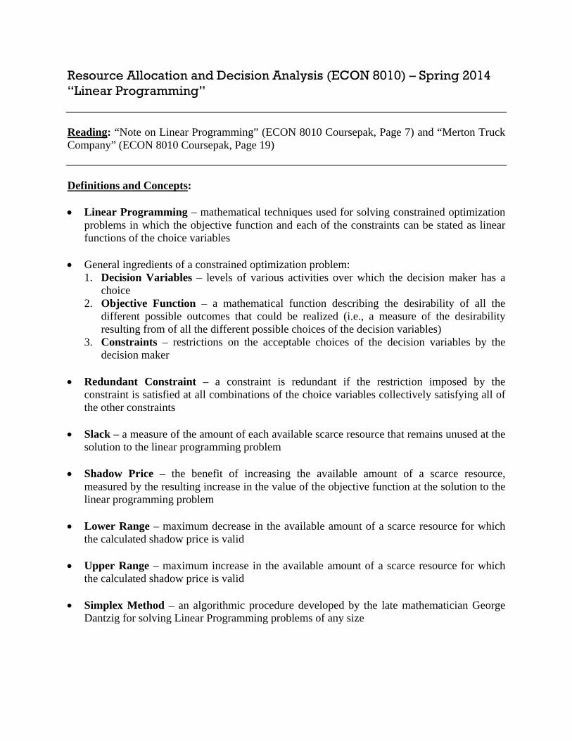
To see that our objective function is indeed linear, let’s illustrate it graphically…

helpful to draw the objective function for varying realized values of production costs

(e.g., 24c , 36c , 60c , and 84c )

note: the slope of each isocost curve is simply

2

1

w

w

so, again, the Objective Function for this problem is clearly linear the goal of the firm is to Minimize Production Costs => they want to be on the isocost

line closest to the origin, while still producing the target level of output

1x0 

0 

“ 84c isocost line” Combinations of the two inputs which cost exactly $8,400 dollars 2x  

“ 60c isocost line” Combinations of the two inputs which cost exactly $6,000 dollars

“ 24c isocost line” Combinations of the two inputs which cost exactly $2,400 dollars

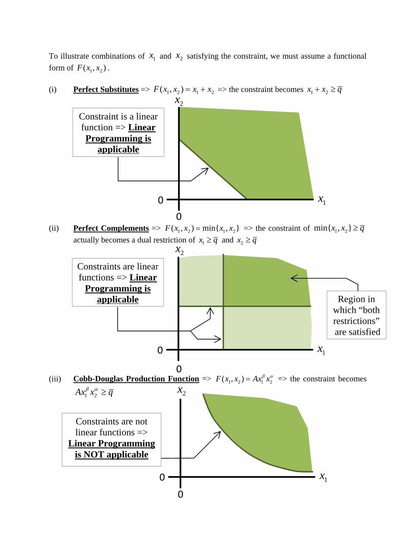
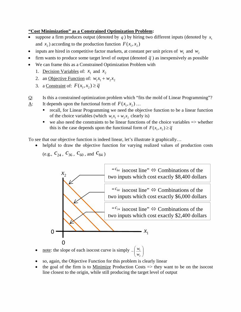
To illustrate combinations of 1x and 2x satisfying the constraint, we must assume a functional

form of ),( 21 xxF . (i) Perfect Substitutes => 2121 ),( xxxxF => the constraint becomes qxx 21

(ii) Perfect Complements => },min{),( 2121 xxxxF => the constraint of qxx },min{ 21

actually becomes a dual restriction of qx 1 and qx 2

(iii) Cobb-Douglas Production Function =>

2121 ),( xAxxxF => the constraint becomes

qxAx 21

1x  0 

0

2x

Constraint is a linear function => Linear Programming is

applicable

1x  0 

0

2x

Constraints are linear functions => Linear

Programming is applicable Region in

which “both restrictions” are satisfied

1x  0 

0

2x

Constraints are not linear functions =>

Linear Programming is NOT applicable

Example 1 – Insulation Production (Coursepak, Page 7): 1. Specify the objective function of the plant manager. 2. State equations for all of the constraints facing the plant manager. 3. Formally state the Linear Programming problem. 4. Graphically illustrate the “feasible set” of the decision variables. 5. Determine the solution to this Linear Programming problem. 1. Specify the objective function of the plant manager.

First recognize that the decision variables can be thought of as “the number of truckloads of ‘Type B’ insulation” (denoted B ) and “the number of truckloads of ‘Type R’ insulation” (denoted R ) Often, we have some flexibility in “how we specify the problem” => we could have

thought of our decision variables as “tons of ‘Type B’ insulation” and “tons of ‘Type R’ insulation”

In this case, there is no “right” or “wrong” approach => either specification will give the correct insights (so long as we are consistent throughout the analysis)

Thus, the objective is to maximize contribution, which is equal to: RB 200,1950 2. State equations for all of the constraints facing the plant manager.

The plant manager faces several restrictions on her choice (i) “…can produce any mix of output, as long as the total weight is no more than 70

tons per day…One truckload of “Type B” insulation weighs 1.4 tons; one truckload of “Type R” weighs 2.8 tons.” => 70)8.2()4.1( RB

(ii) “…loading facilities can handle up to 30 trucks per day” => 30 RB (iii) “…can obtain at most 65 canisters of the (flame retarding) agent per day. One

truckload of (finished) “Type B” insulation requires an input of three canisters of the agent, but one truckload of “Type R” insulation requires only one canister.” =>

653 RB (iv) implicit assumptions of 0B and 0R

3. Formally state the Linear Programming problem.

The plant manager faces the Linear Programming problem of: Maximize RB 200,1950 Subject to:

70)8.2()4.1( RB 30 RB 653 RB

0B and 0R

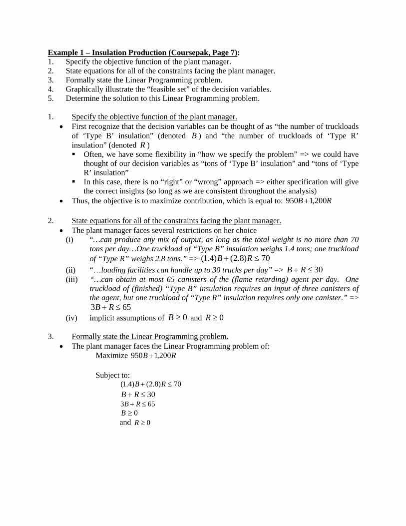
4. Graphically illustrate the “feasible set” of the decision variables.

25)5.(8.2

70

8.2

4.1

BBR

30)1( BR

65)3( BR

B0 0 

R  

Slope of line is equal to (-.5)

50

25 

B0 

0 

R  

Slope of line is equal to (-1)

30

30 

B0 

0 

R  

Slope of line is equal to (-3)

65/3=21.6666…

65 

“Machine Constraint”

“Loading Constraint”

“Flame Retarding

Agent Constraint”

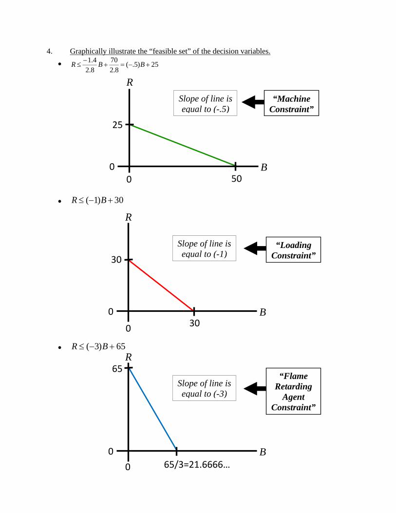
(?) What does the picture look like when we draw all three constraints in the same graph? “horizontal intercepts” can be ranked from smallest to largest as “blue < red < green”… “vertical intercepts” can be ranked from smallest to largest as “green < red < blue”…

But, which of the two following cases do we have?

or To figure this out, start by determining the intersection of “blue” and “green”…

at this intersection 25)5.( BR and 65)3( BR must both be satisfied simultaneously

25)5.(65)3( BB B)5.2(40 165.240 B

From which it follows 1765)16)(3(25)16)(5.( R And then figure out if this point is “above” or “below” “red”…

recall, the equation for “red” is 30)1( BR

thus, if 16B , then 1430)16)(1( R

since 1714 it follows that “red” passes below the point of intersection between “blue” and “green” (i.e., the correct picture is the one above on the left)

B0 

0 

R  

B0 

0 

R

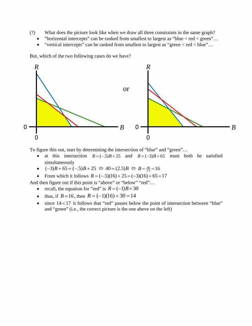
From here we can determine the point of intersection between… “red” and “green” as: 25)5.(30)1( BB 5)5(. B 10B and 20R

“red” and “blue” as: 65)3(30)1( BB 352 B 5.17B and 5.12R Thus, the feasible set is:

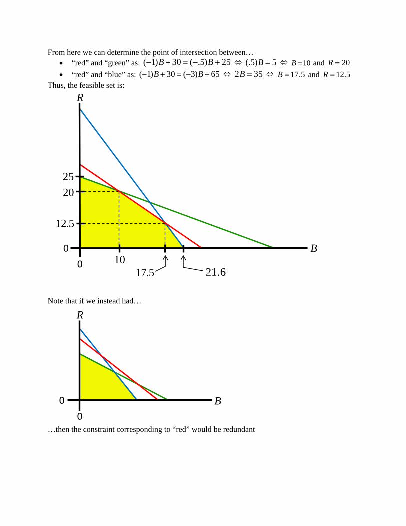
Note that if we instead had…

…then the constraint corresponding to “red” would be redundant

B  0 

0 

R  

6.2110  

5.17  

25  20  

5.12  

B0 

0 

R  

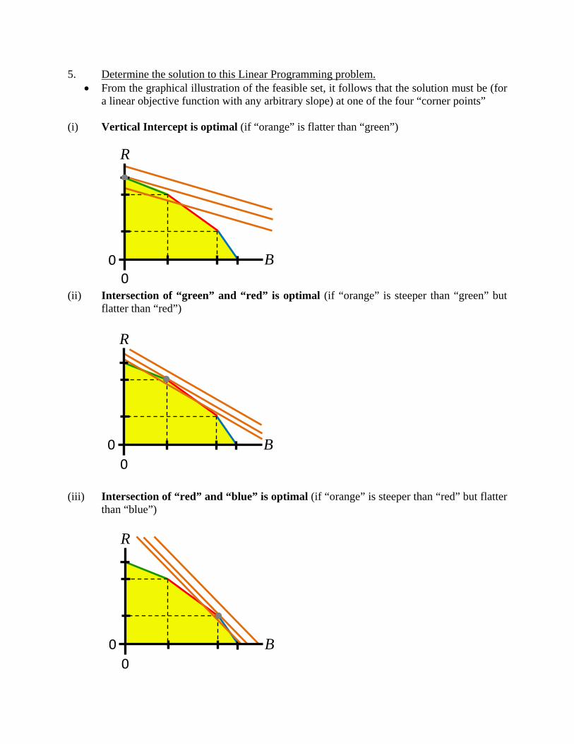
5. Determine the solution to this Linear Programming problem. From the graphical illustration of the feasible set, it follows that the solution must be (for

a linear objective function with any arbitrary slope) at one of the four “corner points” (i) Vertical Intercept is optimal (if “orange” is flatter than “green”)

(ii) Intersection of “green” and “red” is optimal (if “orange” is steeper than “green” but

flatter than “red”)

(iii) Intersection of “red” and “blue” is optimal (if “orange” is steeper than “red” but flatter

than “blue”)

B  0 0 

R  

B  0 

0 

R  

B  0 

0 

R  

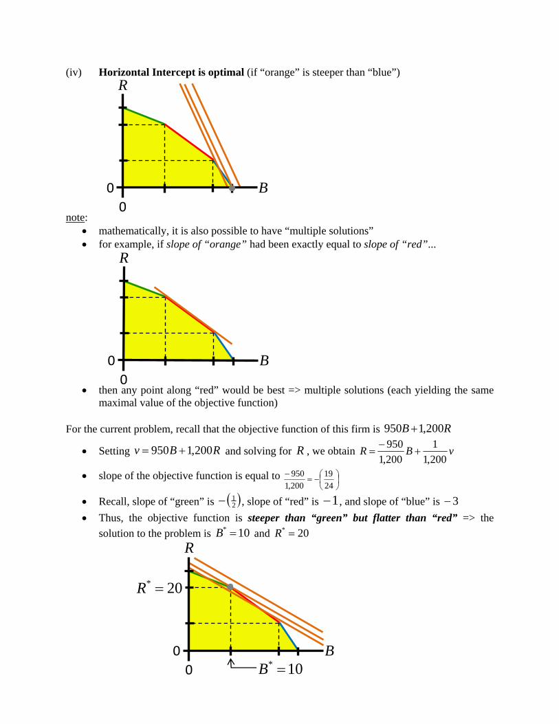
(iv) Horizontal Intercept is optimal (if “orange” is steeper than “blue”)

note:

mathematically, it is also possible to have “multiple solutions” for example, if slope of “orange” had been exactly equal to slope of “red”...

then any point along “red” would be best => multiple solutions (each yielding the same maximal value of the objective function)

For the current problem, recall that the objective function of this firm is RB 200,1950

Setting RBv 200,1950 and solving for R , we obtain vBR200,1

1

200,1

950

slope of the objective function is equal to

24

19

200,1

950

Recall, slope of “green” is 21 , slope of “red” is 1 , and slope of “blue” is 3

Thus, the objective function is steeper than “green” but flatter than “red” => the

solution to the problem is 10* B and 20* R

B  0 

0 

R  

B  0 

0 

R  

10* B

20* R  

B  0 

0 

R  

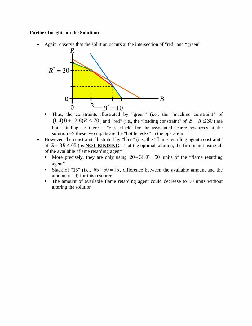
Further Insights on the Solution:

Again, observe that the solution occurs at the intersection of “red” and “green”

Thus, the constraints illustrated by “green” (i.e., the “machine constraint” of 70)8.2()4.1( RB ) and “red” (i.e., the “loading constraint” of 30 RB ) are

both binding => there is “zero slack” for the associated scarce resources at the solution => these two inputs are the “bottlenecks” in the operation

However, the constraint illustrated by “blue” (i.e., the “flame retarding agent constraint” of 653 BR ) is NOT BINDING => at the optimal solution, the firm is not using all of the available “flame retarding agent” More precisely, they are only using 50)10(320 units of the “flame retarding

agent” Slack of “15” (i.e., 155065 , difference between the available amount and the

amount used) for this resource The amount of available flame retarding agent could decrease to 50 units without

altering the solution

B  0 

0 

R  

10* B

20* R  

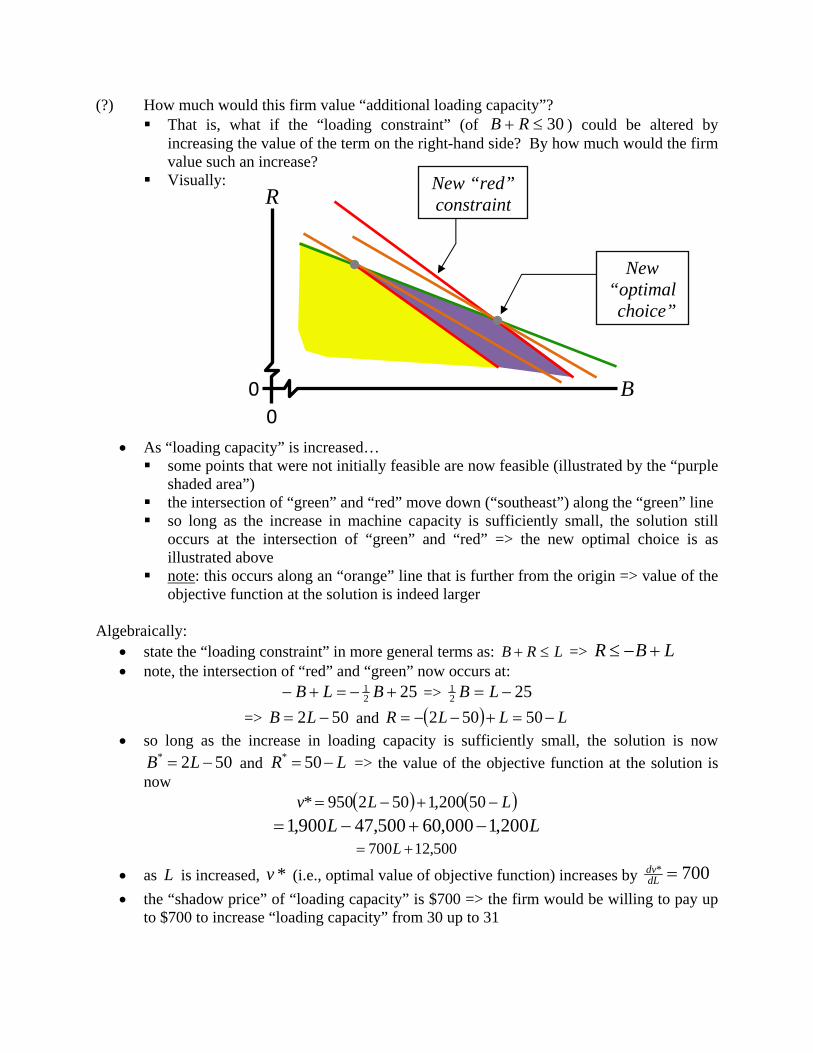
(?) How much would this firm value “additional loading capacity”? That is, what if the “loading constraint” (of 30 RB ) could be altered by

increasing the value of the term on the right-hand side? By how much would the firm value such an increase?

Visually:

As “loading capacity” is increased… some points that were not initially feasible are now feasible (illustrated by the “purple

shaded area”) the intersection of “green” and “red” move down (“southeast”) along the “green” line so long as the increase in machine capacity is sufficiently small, the solution still

occurs at the intersection of “green” and “red” => the new optimal choice is as illustrated above

note: this occurs along an “orange” line that is further from the origin => value of the objective function at the solution is indeed larger

Algebraically:

state the “loading constraint” in more general terms as: LRB => LBR note, the intersection of “red” and “green” now occurs at:

2521 BLB => 252

1 LB

=> 502 LB and LLLR 50502

so long as the increase in loading capacity is sufficiently small, the solution is now

502* LB and LR 50* => the value of the objective function at the solution is now

LLv 50200,1502950*

LL 200,1000,60500,47900,1 500,12700 L

as L is increased, *v (i.e., optimal value of objective function) increases by 700* dLdv

the “shadow price” of “loading capacity” is $700 => the firm would be willing to pay up to $700 to increase “loading capacity” from 30 up to 31

B  0 

0 

R  New “red” constraint

New “optimal choice”

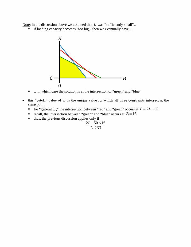
Note: in the discussion above we assumed that L was “sufficiently small”… if loading capacity becomes “too big,” then we eventually have…

…in which case the solution is at the intersection of “green” and “blue”

this “cutoff” value of L is the unique value for which all three constraints intersect at the

same point for “general L ,” the intersection between “red” and “green” occurs at 502 LB recall, the intersection between “green” and “blue” occurs at 16B thus, the previous discussion applies only if

16502 L 33L

B0 

0 

R  

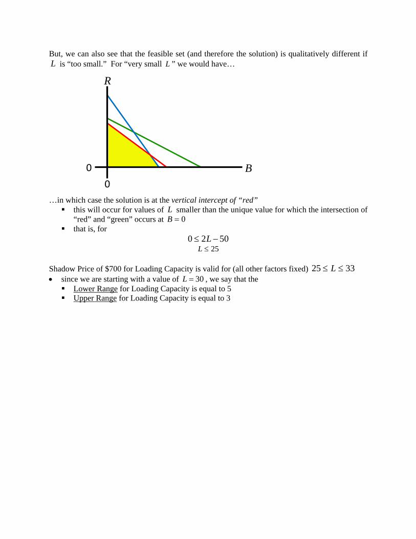
But, we can also see that the feasible set (and therefore the solution) is qualitatively different if L is “too small.” For “very small L ” we would have…

…in which case the solution is at the vertical intercept of “red” this will occur for values of L smaller than the unique value for which the intersection of

“red” and “green” occurs at 0B that is, for

5020 L 25L

Shadow Price of $700 for Loading Capacity is valid for (all other factors fixed) 3325 L since we are starting with a value of 30L , we say that the Lower Range for Loading Capacity is equal to 5 Upper Range for Loading Capacity is equal to 3

B0 

0 

R  

Similarly, for “machine capacity” Algebraically:

state “machine constraint” in more general terms as: MBR 8.21

21

note, the intersection of “red” and “green” now occurs at: MBB 8.2

12130 => MB 8.2

121 30

=> 4.160 MB and 306030 4.14.1 MMR

so long as the increase in machine capacity is sufficiently small, the solution is now

4.1* 60 MB and 304.1

* MR => value of the objective function at the solution is now

30200,160950* 4.14.1 MMv

M4.1250000,21

thus, as M is increased, *v  increases by 57.1784.1250* dM

dv

the “shadow price” of “machine capacity” is $178.57 => the firm would be willing to pay up to $178.57 to increase “machine capacity” from 70 up to 71

Further, it can be shown that

the Lower Range for Machine Capacity is 10.50 the Upper Range for Machine Capacity is 14.00

(?) What about the Shadow Price for the “flame retarding agent”? (A) Start by using “economic intuition”…

recall the definition of “Shadow Price” (benefit of increasing the available amount of a scarce resource, measured by the resulting increase in the value of the objective function at the solution to the linear programming problem)

the constraint on the “flame retarding agent” was NOT BINDING => at the solution, the firm was not using all of the available units of this input

thus, the solution would not change if the available amount of “flame retarding agent” were increased => Shadow Price is equal to zero

further, it follows that the Upper Range for this Shadow Price is infinity (i.e., the shadow price will still equal zero even as the available amount of the “flame retarding agent” is increased to infinity)

Recognize that in general:

if Slack is equal to zero, then Shadow Price will be positive if Slack is positive, then Shadow Price is equal to zero

“Merton Truck Company”: (Page 19 of Coursepak) Choose levels of production for two different types of trucks: 1x (units of Model 101) and

2x (units of Model 102)

Constraints of: Engine Assembly constraint: 000,42 21 xx

Metal Stamping constraint: 000,622 21 xx

Model 101 Assembly constraint: 000,52 1 x

Model 102 Assembly constraint: 500,43 2 x Objective: maximize contribution Per Unit Costs for Model 101 of:

(materials) + (labor) + (variable overhead) = $24,000 + $4,000 + $8,000 = $36,000 Per Unit Revenue for Model 101 of $39,000 Per Unit Costs for Model 102 of:

(materials)+(labor)+(variable overhead) = $20,000 + $4,500 + $8,500 = $33,000 Per Unit Revenue for Model 102 of $38,000

Thus, the Objective Function is: 21 000,5000,3 xxv Questions:

1a. Find the best product mix for Merton. 1b. Determine the Shadow Price of engine assembly capacity. 1d. Determine the Upper Range for the shadow price of engine assembly capacity

determined in (1b). 2. Merton’s production manager suggests purchasing Model 101 or Model 102 engines

form an outside supplier in order to relieve the capacity problem in the engine assembly department. If Merton decides to pursue this alternative, it will be effectively “renting” capacity: furnishing the necessary materials and engine components, and reimbursing the outside supplier for labor and overhead. Should the company adopt this alternative? If so, what is the maximum rent it should be willing to pay for a machine-hour of engine assembly capacity? What is the maximum number of machine hours it should rent?

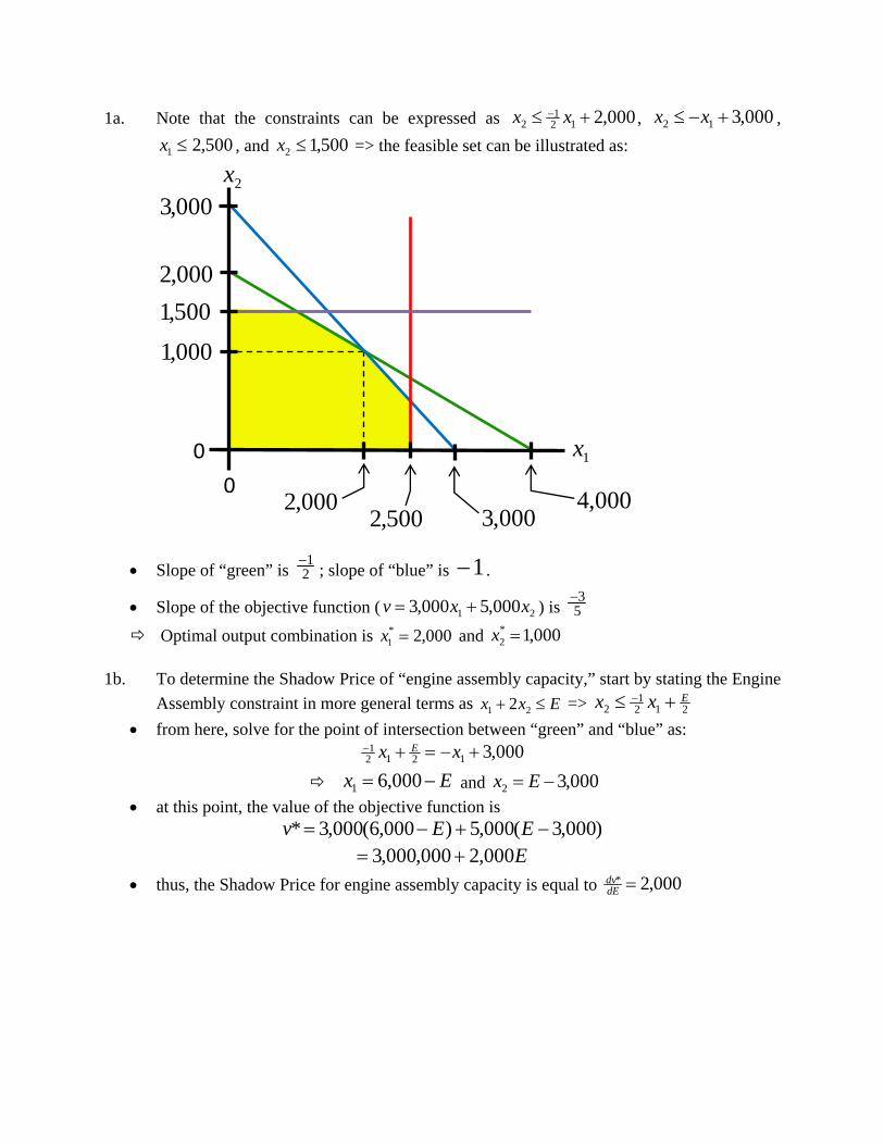
1a. Note that the constraints can be expressed as 000,2121

2 xx , 000,312 xx ,

500,21 x , and 500,12 x => the feasible set can be illustrated as:

Slope of “green” is 21

; slope of “blue” is 1 .

Slope of the objective function ( 21 000,5000,3 xxv ) is 53

Optimal output combination is 000,2*1 x and 000,1*

2 x 1b. To determine the Shadow Price of “engine assembly capacity,” start by stating the Engine

Assembly constraint in more general terms as Exx 21 2 => 2121

2Exx

from here, solve for the point of intersection between “green” and “blue” as: 000,31212

1 xx E

Ex 000,61 and 000,32 Ex

at this point, the value of the objective function is )000,3(000,5)000,6(000,3* EEv

E000,2000,000,3

thus, the Shadow Price for engine assembly capacity is equal to 000,2* dEdv

1x0 

0 000,4  

000,3000,2  

000,2  

000,3  

000,1  

2x  

500,2

500,1  

1d. As “engine assembly capacity” is increased, “green” shifts outward… the solution is still at the intersection of “green” and “blue” until “green” shifts out

beyond the intersection of “blue” and “purple” the intersection of “blue” and “purple” occurs at

000,3500,1 1 x => 500,11 x

thus, the solution is still at the intersection of “green” and “blue” so long as 500,1000,6 E 500,4E

starting at 000,4E , the value of E could increase by 500 and the Shadow Price of 2,000 still applies (i.e., the Upper Range for the Shadow Price is 500)

2. Based upon the answers to (1b) and (1d), Merton should be willing to pay up to $2,000

per unit to rent additional “engine assembly capacity,” up to a maximum of 500 units of engine assembly capacity.

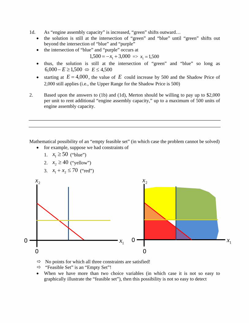
Mathematical possibility of an “empty feasible set” (in which case the problem cannot be solved)

for example, suppose we had constraints of

1. 501 x (“blue”)

2. 402 x (“yellow”)

3. 7021 xx (“red”)

No points for which all three constraints are satisfied! “Feasible Set” is an “Empty Set”! When we have more than two choice variables (in which case it is not so easy to

graphically illustrate the “feasible set”), then this possibility is not so easy to detect

2x  

0  1x

0 

2x

0 

0  1x

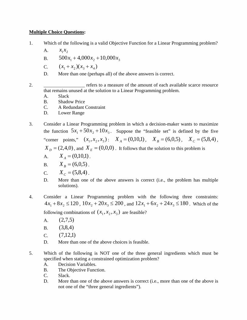
Multiple Choice Questions: 1. Which of the following is a valid Objective Function for a Linear Programming problem?

A. 21xx

B. 321 000,10000,4500 xxx

C. ))(( 4321 xxxx

D. More than one (perhaps all) of the above answers is correct. 2. _________________ refers to a measure of the amount of each available scarce resource

that remains unused at the solution to a Linear Programming problem. A. Slack B. Shadow Price C. A Redundant Constraint D. Lower Range

3. Consider a Linear Programming problem in which a decision-maker wants to maximize

the function 321 10505 xxx . Suppose the “feasible set” is defined by the five

“corner points,” ),,( 321 xxx : )1,10,0(AX , )5,0,6(BX , )4,8,5(CX ,

)0,4,2(DX , and )0,0,0(EX . It follows that the solution to this problem is

A. )1,10,0(AX .

B. )5,0,6(BX .

C. )4,8,5(CX .

D. More than one of the above answers is correct (i.e., the problem has multiple solutions).

4. Consider a Linear Programming problem with the following three constraints:

12084 21 xx , 2002010 32 xx , and 18024612 321 xxx . Which of the

following combinations of ),,( 321 xxx are feasible?

A. )5,7,2(

B. )4,8,3(

C. )1,12,7( D. More than one of the above choices is feasible. 5. Which of the following is NOT one of the three general ingredients which must be

specified when stating a constrained optimization problem? A. Decision Variables. B. The Objective Function. C. Slack.

D. More than one of the above answers is correct (i.e., more than one of the above is not one of the “three general ingredients”).

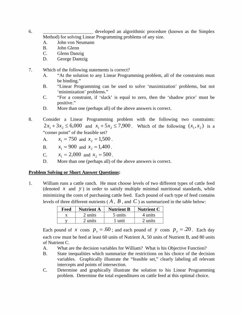
6. _____________________ developed an algorithmic procedure (known as the Simplex Method) for solving Linear Programming problems of any size.

A. John von Neumann B. John Glenn

C. Glenn Danzig D. George Dantzig 7. Which of the following statements is correct?

A. “At the solution to any Linear Programming problem, all of the constraints must be binding.”

B. “Linear Programming can be used to solve ‘maximization’ problems, but not ‘minimization’ problems.”

C. “For a constraint, if ‘slack’ is equal to zero, then the ‘shadow price’ must be positive.”

D. More than one (perhaps all) of the above answers is correct. 8. Consider a Linear Programming problem with the following two constraints:

000,632 21 xx and 900,75 21 xx . Which of the following ),( 21 xx is a “corner point” of the feasible set?

A. 7501 x and 500,12 x .

B. 9001 x and 400,12 x .

C. 000,21 x and 5002 x . D. More than one (perhaps all) of the above answers is correct. Problem Solving or Short Answer Questions: 1. William runs a cattle ranch. He must choose levels of two different types of cattle feed

(denoted x and y ) in order to satisfy multiple minimal nutritional standards, while minimizing the costs of purchasing cattle feed. Each pound of each type of feed contains levels of three different nutrients ( A , B , and C ) as summarized in the table below:

Feed Nutrient A Nutrient B Nutrient C x 2 units 5 units 4 units y 2 units 1 unit 2 units

Each pound of x costs 60.xp ; and each pound of y costs 20.yp . Each day

each cow must be feed at least 60 units of Nutrient A, 50 units of Nutrient B, and 80 units of Nutrient C. A. What are the decision variables for William? What is his Objective Function? B. State inequalities which summarize the restrictions on his choice of the decision

variables. Graphically illustrate the “feasible set,” clearly labeling all relevant intercepts and points of intersection.

C. Determine and graphically illustrate the solution to his Linear Programming problem. Determine the total expenditures on cattle feed at this optimal choice.

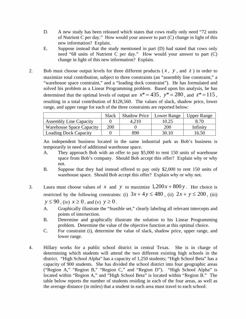
D. A new study has been released which states that cows really only need “72 units of Nutrient C per day.” How would your answer to part (C) change in light of this new information? Explain.

E. Suppose instead that the study mentioned in part (D) had stated that cows only need “68 units of Nutrient C per day.” How would your answer to part (C) change in light of this new information? Explain.

2. Bob must choose output levels for three different products ( x , y , and z ) in order to

maximize total contribution, subject to three constraints (an “assembly line constraint,” a “warehouse space constraint,” and a “loading dock constraint”). He has formulated and solved his problem as a Linear Programming problem. Based upon his analysis, he has determined that the optimal levels of output are 435* x , 280* y , and 115* z , resulting in a total contribution of $128,560. The values of slack, shadow price, lower range, and upper range for each of the three constraints are reported below:

Slack Shadow Price Lower Range Upper Range Assembly Line Capacity 0 4,210 10.25 8.70 Warehouse Space Capacity 200 0 200 Infinity Loading Dock Capacity 0 890 30.10 16.50

An independent business located in the same industrial park as Bob’s business is temporarily in need of additional warehouse space. A. They approach Bob with an offer to pay $5,000 to rent 150 units of warehouse

space from Bob’s company. Should Bob accept this offer? Explain why or why not.

B. Suppose that they had instead offered to pay only $2,000 to rent 150 units of warehouse space. Should Bob accept this offer? Explain why or why not.

3. Laura must choose values of x and y to maximize yx 800200,1 . Her choice is

restricted by the following constraints: (i) 48043 yx , (ii) 2002 yx , (iii)

90y , (iv) 0x , and (v) 0y . A. Graphically illustrate the “feasible set,” clearly labeling all relevant intercepts and

points of intersection. B. Determine and graphically illustrate the solution to his Linear Programming

problem. Determine the value of the objective function at this optimal choice. C. For constraint (i), determine the value of slack, shadow price, upper range, and

lower range. 4. Hillary works for a public school district in central Texas. She is in charge of

determining which students will attend the two different existing high schools in the district. “High School Alpha” has a capacity of 1,250 students; “High School Beta” has a capacity of 900 students. She has divided the school district into four geographic areas (“Region A,” “Region B,” “Region C,” and “Region D”). “High School Alpha” is located within “Region A,” and “High School Beta” is located within “Region B.” The table below reports the number of students residing in each of the four areas, as well as the average distance (in miles) that a student in each area must travel to each school:

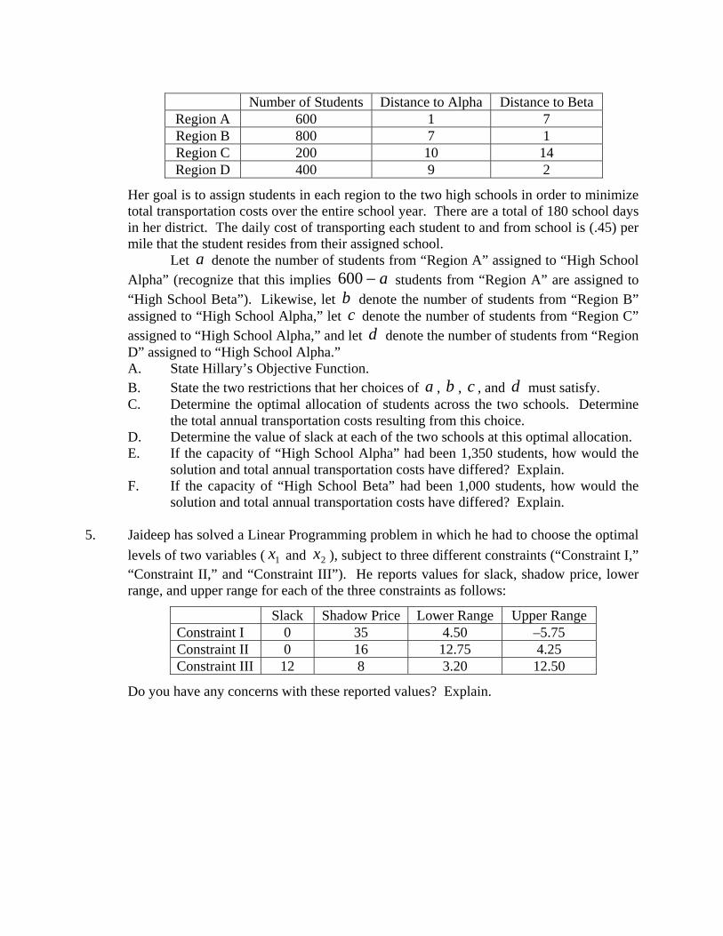
Number of Students Distance to Alpha Distance to Beta Region A 600 1 7 Region B 800 7 1 Region C 200 10 14 Region D 400 9 2

Her goal is to assign students in each region to the two high schools in order to minimize total transportation costs over the entire school year. There are a total of 180 school days in her district. The daily cost of transporting each student to and from school is (.45) per mile that the student resides from their assigned school.

Let a denote the number of students from “Region A” assigned to “High School Alpha” (recognize that this implies a600 students from “Region A” are assigned to “High School Beta”). Likewise, let b denote the number of students from “Region B” assigned to “High School Alpha,” let c denote the number of students from “Region C” assigned to “High School Alpha,” and let d denote the number of students from “Region D” assigned to “High School Alpha.” A. State Hillary’s Objective Function. B. State the two restrictions that her choices of a , b , c , and d must satisfy. C. Determine the optimal allocation of students across the two schools. Determine

the total annual transportation costs resulting from this choice. D. Determine the value of slack at each of the two schools at this optimal allocation. E. If the capacity of “High School Alpha” had been 1,350 students, how would the

solution and total annual transportation costs have differed? Explain. F. If the capacity of “High School Beta” had been 1,000 students, how would the

solution and total annual transportation costs have differed? Explain. 5. Jaideep has solved a Linear Programming problem in which he had to choose the optimal

levels of two variables ( 1x and 2x ), subject to three different constraints (“Constraint I,” “Constraint II,” and “Constraint III”). He reports values for slack, shadow price, lower range, and upper range for each of the three constraints as follows:

Slack Shadow Price Lower Range Upper Range Constraint I 0 35 4.50 –5.75 Constraint II 0 16 12.75 4.25 Constraint III 12 8 3.20 12.50

Do you have any concerns with these reported values? Explain.

Answers to Multiple Choice Questions:

1. B 2. A 3. A 4. B 5. C 6. D 7. C 8. B

Answers to Problem Solving or Short Answer Questions: 1A. His decision variables are x (pounds of “feed x”) and y (pounds of “feed y”). His

Objective Function is: yxypxp yx )2(.)6(. (the value of which he aims to

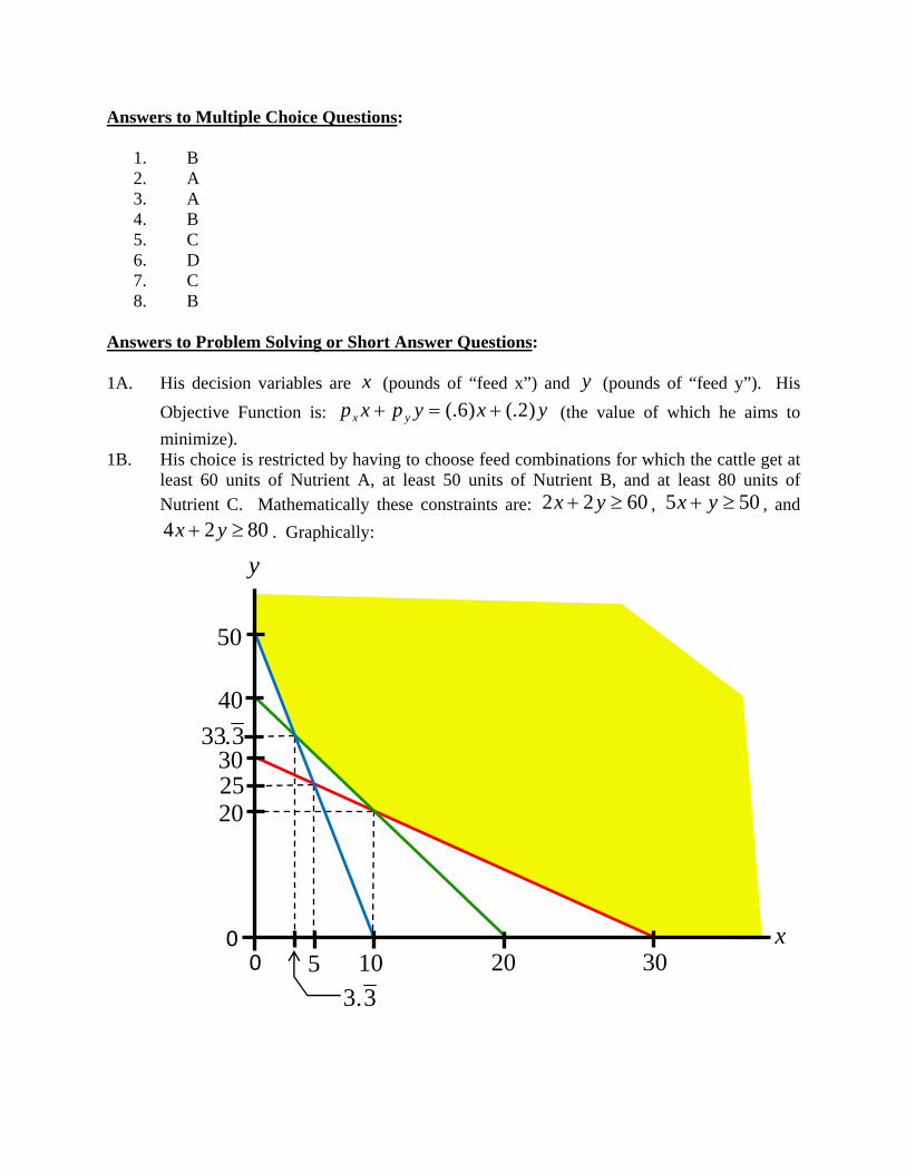
minimize). 1B. His choice is restricted by having to choose feed combinations for which the cattle get at

least 60 units of Nutrient A, at least 50 units of Nutrient B, and at least 80 units of Nutrient C. Mathematically these constraints are: 6022 yx , 505 yx , and

8024 yx . Graphically:

x0 0 

y  

30  10 20

40  

30 

50  

25  20  

5  

3.33  

3.3

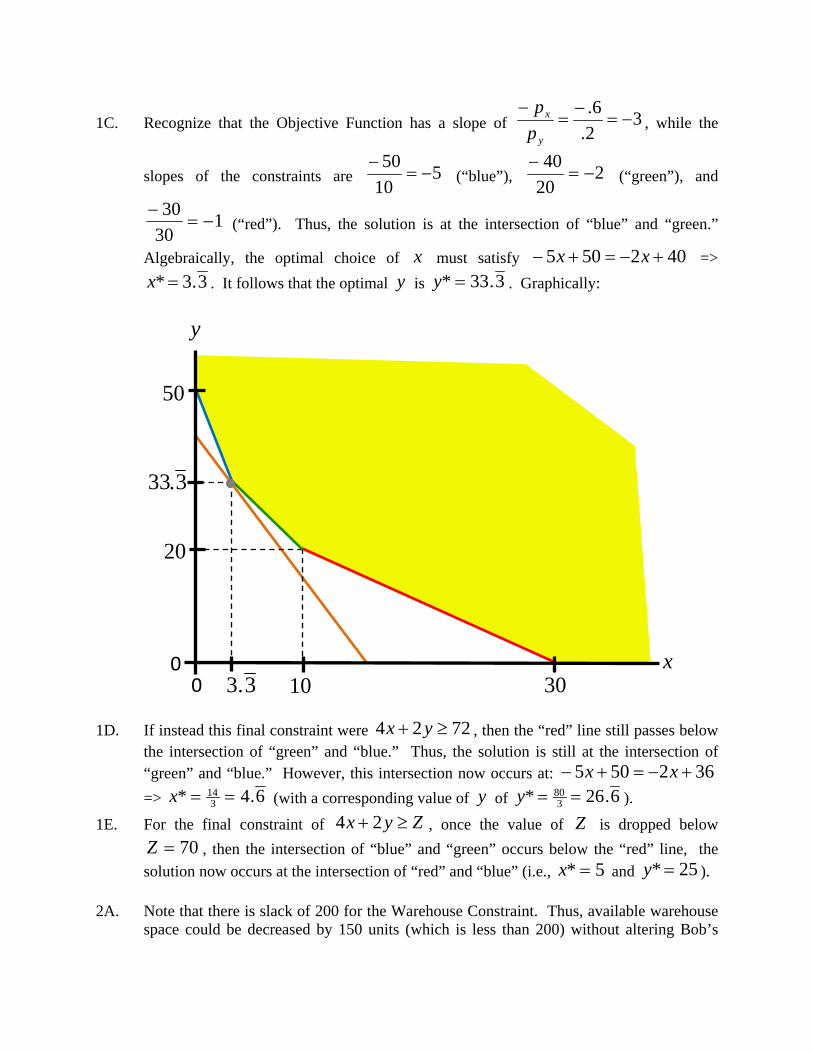
1C. Recognize that the Objective Function has a slope of 32.

6.

y

x

p

p, while the

slopes of the constraints are 510

50

(“blue”), 2

20

40

(“green”), and

130

30

(“red”). Thus, the solution is at the intersection of “blue” and “green.”

Algebraically, the optimal choice of x must satisfy 402505 xx =>

3.3* x . It follows that the optimal y is 3.33* y . Graphically: 1D. If instead this final constraint were 7224 yx , then the “red” line still passes below

the intersection of “green” and “blue.” Thus, the solution is still at the intersection of “green” and “blue.” However, this intersection now occurs at: 362505 xx

=> 6.4* 314 x (with a corresponding value of y  of 6.26* 3

80 y ).

1E. For the final constraint of Zyx 24 , once the value of Z is dropped below

70Z , then the intersection of “blue” and “green” occurs below the “red” line, the

solution now occurs at the intersection of “red” and “blue” (i.e., 5* x and 25* y ). 2A. Note that there is slack of 200 for the Warehouse Constraint. Thus, available warehouse

space could be decreased by 150 units (which is less than 200) without altering Bob’s

x0 0 

y  

3010  

50  

20  

3.33  

3.3  

optimal choice. Because of this, he should be willing to accept $5,000 for these unused 150 units of warehouse space.

2B. Based upon the logic above, if he were made a “take-it-or-leave-it” offer for any amount of warehouse space up to 200 units for any positive payment, then he should accept the offer. So, he should be willing to accept this even lower amount of only $2,000 for these 150 units of warehouse space.

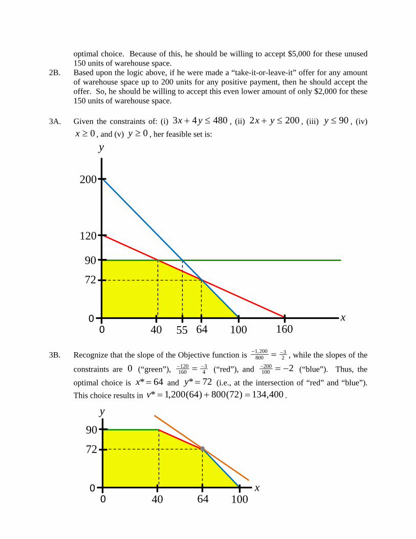
3A. Given the constraints of: (i) 48043 yx , (ii) 2002 yx , (iii) 90y , (iv)

0x , and (v) 0y , her feasible set is:

3B. Recognize that the slope of the Objective function is 23

800200,1 , while the slopes of the

constraints are 0 (“green”), 43

160120 (“red”), and 2100

200 (“blue”). Thus, the

optimal choice is 64* x and 72* y (i.e., at the intersection of “red” and “blue”).

This choice results in 400,134)72(800)64(200,1* v .

x0 0 

y  

160  40   100

72  

120 

200  

90 

55 64

x0 0 

y  

40   100

72  

90 

64

3C. Constraint (i) ( 48043 yx , illustrated by the “red” line) is binding. Thus, slack is equal to 0. The solution will still occur at the intersection of “red” and “blue” so long as “red” intersects “blue” at a point with 10055 x . Expressing this constraint in more

general terms as iZyx 43 (or equivalently as 443 iZxy ), the intersection

between “red” and “blue” occurs at 2002443 xx iZ

=> 5160 iZx . Thus,

this intersection occurs at 10055 x so long as 525300 iZ . Starting with

480iZ , it follows that the Upper Range is 45 and the Lower Range is 180. Finally,

for 525300 iZ , the solution is 5160* iZx and 120* 52 iZy , for which

000,9680120800160200,1* 52

5 iZZ Zv ii . Thus, the Shadow Price

is equal to 80* idZ

dv .

4A. Hillary’s Objective Function is

)400(29)200(1410)800(17)600(71)45)(.180( ddccbbaa ddccbbaa 2800914800,21080077200,481 dcba 7466600,881

She aims to minimize the value of this function. 4B. Her choice is restricted by the capacity of each school. For chosen values of a , b , c ,

and d , the total number of students attending “High School alpha” is simply dcba . Recall, the capacity of this school is 1,250 students. Thus, she faces a

constraint of 250,1 dcba . Similarly, the total number of students attending

“High School Beta” is )400()200()800()600( dcba , which can

be simplified to )(000,2 dcba . Since the capacity of “High School Beta” is

900 students, this implies a restriction of 900)(000,2 dcba =>

dcba 100,1 .

4C. If the only restrictions on her choice were that 6000 a , 8000 b , 2000 c , and 4000 d , then she would clearly minimize the value of the

objective function by choosing that 600a , 0b , 200c , and 0d . However,

this choice would violate the constraint of dcba 100,1 (since it would assign 1,200 students to “High School Beta,” a school with a capacity of only 900 students). From here, in order to identify the solution to the constrained optimization problem, she must reassign 300 students from “High School Beta” to “High School Alpha.” The two types of students that should could potentially reassign are either “Region B” students or “Region D” students. Reassigning one “Region D” student will increase the value of the Objective Function by ($81)(7)=$567, whereas reassigning one “Region B” student will increase the value of the Objective Function by only ($81)(6)=$486. Since she wants to minimize the value of the Objective Function the best choice is to reassign 300 “Region B” students from “High School Beta” to “High School Alpha.” Thus, her optimal choice

is 600a , 300b , 200c , and 0d , which gives rise to annual transportation

costs of 000,486)000,6(810800800,1600,3600,881 . 4D. At the optimal choice 1,100 students are assigned to “High School Alpha.” Since this

school has a capacity of 1,250 students, slack is equal to 150. At the optimal choice 900 students are assigned to “High School Beta.” Since this school has a capacity of 900 students, slack is equal to 0.

4E. Increasing the availability of a scarce resource for which slack is positive at the solution to the Linear Programming problem will in general not alter the solution. Thus, if the capacity of “High School Alpha” had been 1,350 students (instead of 1,250 students), the solution would not differ at all.

4F. At the initial solution, “High School Beta” is filled to capacity. Thus, increasing capacity of this school should alter the solution to the problem (and ultimately lead to a lower value of the objective function). If the capacity had been 1,000 instead of only 900, then the second constraint is 000,1)(000,2 dcba => dcba 000,1 . Thus (applying the same logic used in answering part (4C) above), the optimal choice is

600a , 200b , 200c , and 0d . This choice leads to annual transportation

costs of 400,437)400,5(810800200,1600,3600,881 . Thus, having this extra capacity at “High School Beta” would allow the district to realize transportation costs that are $48,600 less per year.

5. Based upon the reported values, there appear to be some mistakes in his results. First,

“Upper Range” specifies the maximum increase in the available amount of a scarce resource for which the calculated shadow price is valid. The value of “Upper Range” should always be greater than or equal to zero. Thus, the reported value of (–5.75) for “Constraint I” is not an acceptable value for “Upper Range.” Second, it must always be true that if “slack” is positive, then the corresponding shadow price is equal to zero. This is not true for the values reported above corresponding to “Constraint III” (suggesting an additional error).