Embed Size (px)
Citation preview

1
Resonant Interaction of a Rectangular Jet with a Flat-plate
K.B.M.Q. Zaman1, A. F. Fagan
2, M. M. Clem
3 and C. A. Brown
4
NASA Glenn Research Center
Cleveland, OH 44135
Abstract
A resonant interaction between a large aspect ratio rectangular jet and a flat-plate is addressed in this
experimental study. The plate is placed parallel to but away from the direct path of the jet. At high subsonic
conditions and for certain relative locations of the plate, the resonance accompanied by an audible tone is
encountered. The trends of the tone frequency variation exhibit some similarities to, but also marked
differences from, corresponding trends of the well-known edgetone phenomenon. Under the resonant
condition flow visualization indicates a periodic flapping motion of the jet column. Phase-averaged Mach
number data obtained near the plate’s trailing edge illustrate that the jet cross-section goes through large
contortions within the period of the tone. Farther downstream a clear ‘axis switching’ takes place. These
results suggest that the assumption of two-dimensionality should be viewed with caution in any analysis of
the flow.
1. Introduction
Prompted by noise reduction goals, some newer aircraft concepts involve over-the-wing engine designs which
provide a shielding effect for the jet noise propagated towards the ground. Such a configuration is also desired from
the point of view of sonic boom reduction with supersonic flight since the shock waves from the engine
components would be directed upwards rather than towards the ground. In these concepts rectangular geometries
for the jet nozzle are preferred for ease of integration with the airframe and also for possible noise benefits inherent
to the non-axisymmetric geometry [1-4]. However, in many cases the flow just downstream of the nozzle is close to
a surface before emanating as a free jet. In those cases jet-surface interaction becomes an important issue. A
research program was initiated to investigate this experimentally, computationally as well as analytically. Plans
were developed for detailed experiments in the Aeroacoustics Propulsion Laboratory (AAPL) of NASA Glenn
Research Center (GRC). In support of these plans, and in order to provide a database for an ongoing analytical
effort [5, 6] in a timely manner, it was decided that a preliminary experiment be carried out in a relatively smaller
facility during the Fall of 2012. Hot-wire surveys at low Mach numbers and Pitot-probe surveys at high Mach
numbers together with limited noise measurements for both the ‘reflected’ and ‘shielded’ sides of the plate were
conducted. The results were summarized in [7].
During the course of the latter experiments, an unexpected resonant interaction was encountered. It occurred for
certain ranges of the plate’s location relative to the nozzle and at high subsonic Mach numbers. It was accompanied
by audible tones that obviously had an impact on the radiated noise. It also impacted the flowfield in a profound
manner in that the jet cross-section went through an ‘axis switching’ which otherwise did not occur in the absence
of the tone. An understanding of the resonant interaction was important not only to guide future research under the
program but also so that it could be avoided or suppressed in possible future applications.
The resonance phenomenon studied subsequently, in the same smaller facility, is the focus of the present paper. A
parametric study was conducted by varying the jet Mach number and the plate’s streamwise as well as lateral
locations. This was done for plates of varying streamwise lengths as elaborated further in the next section. Note that
1 Inlet & Nozzle Branch, Aeropropulsion Division, AIAA Associate Fellow.
2 Optical Instrumentation Branch, Instrumentation and Controls Division, AIAA member.
3 Optical Instrumentation Branch, Instrumentation and Controls Division, AIAA member.
4 Acoustics Branch, Aeropropulsion Division, AIAA member.
https://ntrs.nasa.gov/search.jsp?R=20150006757 2020-05-11T03:58:38+00:00Z

2
with diminishing streamwise length the interacting surface was no longer a ‘plate’, however, the effect of the plate
length was deemed important in order to obtain a better understanding of the phenomenon. Note also that all data
presented herein pertain to having the plate placed on one side of the jet but avoiding a direct impact from the jet’s
core flow. In this respect, the phenomenon under study is different from the well-known edgetone phenomenon [8-
10]. The latter involves a wedge placed symmetrically in the middle of the jet. Frequency data from the present
experiment will be compared with edgetone data in the following. The experimental procedure and parameters
tested will be described first, followed by discussion of key results and concluding remarks.
2. Experimental Facility and Procedure
An open jet facility (‘CW17’) at NASA GRC is used for this study [11]. Compressed air passes through a
30” diameter plenum chamber before exhausting through the nozzle into the ambient of the test chamber.
Only cold (unheated) flow is available and flow visualization as well as detailed flow field surveys by hot-
wire anemometry and Pitot-static probes are possible. With a suitable transition section, the same nozzles
used in the AAPL can be investigated in this facility and vice versa. An 8:1 aspect ratio nozzle, referred to as
‘NA8Z’ in [12] and simply as ‘R8’ in the following, is used for the present experiments. It is one of several nozzles
that, in combination with different surface geometries, were to be studied in the AAPL experimental program. The
design considerations for a class of rectangular nozzles including the R8 have been discussed in [12]. Detailed co-
ordinates for the nozzle, suitable for adaptation in numerical simulation, can also be found in [11]. The nozzle exit
has dimensions of 5.339”x0.658” and thus an equivalent diameter, D=2.12”. Because plates of different lengths are
used in the study and since there is an ambiguity whether the equivalent diameter or the long or the short dimension
of the nozzle is the appropriate length scale, the results are presented simply in dimensional form with unit of
distance in inches.
The experiment was started with a ½”-thick 24”-wide aluminum plate that was 12” long in the streamwise
direction. The trailing edge (TE) of the plate had a 45˚ bevel while the leading edge was square. By reversing the
plate’s orientation it was determined that the two shapes for the trailing edge produced similar resonance with
practically identical noise spectra. Thus, a square trailing edge was chosen for all later experiments that made the
fabrication process easier. Figure 1(a) is a photograph of the overall setup for the experiment. Plates of varying
streamwise lengths (L, ranging from 12” to 1”; Fig. 1b) were used; all plates were ½” thick and 24” in width. An
L=16” plate was also tried but hardware constraints limited the transverse positioning relative to the nozzle. For
brevity, mostly data for the 12”, 8” and 4” long plates (denoted as ‘12L’, ‘8L’ and ‘4L’ cases) are discussed in the
following. In addition, data for a knife edge placed vertically, denoted as the ‘0L’ case, are also included in the
discussion (Fig. 1c). The schematic in Fig. 1(b) also shows the coordinate system used.
For all data, the plate is placed aligned with the nozzle’s long edge, centered in the lateral direction (y) relative to
the jet axis, and parallel to the x-y plane. The transverse (z) location of the plate could be varied manually using
a heavy duty ‘lab-jack’ (located between the breadboards marked 6 and 7 in Fig. 1a). The axial (x) location
could also be varied manually in coarse steps by sliding the assembly on breadboard 7. At the start of the
experiment, attempts were made to mount the plate assembly on a traversing mechanism so that the surveys
could be done under automated computer control. However, the idea had to be abandoned due to structural
vibration concerns, as discussed further with the results.
The test cell has acoustic linings on the ceiling and upper walls and with proper preparation limited noise
measurements are possible. A discussion of the quality of the noise data is given in [7]. Here, the precise
amplitudes of the sound pressure level spectra are of little concern since the study focuses mainly on the
parametric dependence of the resonant tone and its frequency. All noise data presented in the following
pertain to an angular location, =60˚; is referenced with respect to the jet’s downstream axis. Preliminary
surveys showed that the tone was detected most prominently around this location. Microphones (¼-inch,
B&K 4135) held fixed on an overhead arm were used for these measurements. The 60˚ microphone was
50.1” away from nozzle’s exit. Spectral analysis was done over 0-10kHz with a bandwidth of 25 Hz; the
bandwidth primarily dictated the uncertainty in the measurement of the tone frequency.

3
A projection focusing schlieren system, developed by MetroLaser, Inc., was used for flow visualization. The
system is based on a lens and grid technique where a source grid is projected onto a retro-reflective screen
and imaged onto a cut-off grid creating the schlieren effect [13]. Both the source and cut-off grids consist of
identical Ronchi rulings and reside on the same side of the flowfield. The light source illuminating the source
grid is a 5 Watt Xenon flashlamp with 1 micro-second pulse duration. A series of lenses projects an image of
the grid and another set of identical lenses re-images the projected grid onto the cut-off grid. Refractive index
gradients due to density variations in the flow cause the light rays to bend or refract. The cut-off grid, which
is analogous to the “knife-edge” in a classical schlieren system, causes these disturbances to be seen as light
or dark regions in the image of the flow that is captured on a camera sensor located somewhere behind the
cut-off grid. All optical components, as well as the scientific-grade CCD camera (Imperx model IGV-
B4020M), are securely housed in a 23”x17”x10” case (item 10 in Fig. 1a). The case is placed on one side of
the jet while the 30” x 24” retro-reflective screen is placed on the other side. The distances of the two items
from the jet’s center plane dictate the size of the field of view. The chosen distances, within the constraints of
the test chamber, provided a field of view that extended approximately 9” in the streamwise direction. The
thickness of the focused field (in y-direction) was estimated to be about 3”. The pictures shown in the
following are essentially instantaneous snapshots of the flowfield capturing the unsteady vortical structures
as well as shocks in supersonic cases.
Steady-state flowfield surveys are done with a rake of three Pitot probes. The spacing of the probes in y is
0.48” and this is the spatial resolution in that direction for those measurements. Mean Mach number data are
acquired over the cross-sectional (y-z) plane and the data are nondimensionalized by the ‘jet Mach number’,
Mj, as defined below. During the surveys, even though the plenum pressure was held by automated feedback
control, fluctuations occurred depending on other facilities using the ‘central air supply’. This contributed to
the largest uncertainty in the plenum pressure. However, the Mach number data are normalized by the
‘current’ jet Mach number (Mj) calculated from the plenum pressure (p0) read simultaneously with the Pitot
data. The rms fluctuation in Mj (in percent of average Mj), calculated over an entire run, was less than 0.5%
for all data shown. The jet Mach number is calculated from the plenum pressure (p0) and the ambient
pressure (pa) via the isentropic relation, 2/1/)1(
0 )1
2)1)/(((
aj ppM , where is the ratio of specific heats
for air. A jet Mach number range from 0.5 to over 1.0 is covered in the experiment.
The unsteady flowfield surveys are done with a miniature pressure transducer (Endevco 8507c-15). It is
mounted at the end of a 9” long support that telescoped from a root diameter of 0.25” to a sensor diameter of
0.063”. It is inserted straight into the flow, as with a Pitot probe. The probe essentially responded to unsteady
total pressure. During the process of mounting the probe with the telescoping tubes the calibration changed
somewhat from manufacturer specification, as evident upon a check with a piston phone. Estimated
calibration was used and the amplitudes of the unsteady flow data should be considered qualitative.
3. Results
At the start of this investigation structural vibrations were encountered affecting the noise spectra. Such effects were
suspected when the frequency of a spectral peak would not change upon variation of Mj, and confirmed when the
amplitude of the spectral peak changed upon addition of stiffeners to the plate assembly. It was imperative to isolate
these effects, first, in order to confirm that the resonant tones were not due to structural vibration and then for
studying their fluid dynamic characteristics. The approach taken to resolve this issue was to progressively add the
stiffeners to the plate and its mounting structure until the noise spectra did not change any more.
At first, the plate was mounted on a pair of posts placed symmetrically on its major axis. This pair, marked ‘3’ in
Fig. 1(a), can be seen underneath the plate between two other pairs, marked 4 and 5. (In each pair the nearer post is
marked and the two in a given pair are placed symmetrically about the x-z plane). Pairs 4 and 5 were added later as
described in the following. The plate was firmly bolted to the 1-1/2 inch diameter posts of pair 3 and thought to be

4
rigid enough for the experiment. However, a peak around 500Hz appeared consistently in the noise spectra. This
appeared to be the same frequency at which the plate would ‘sing’ upon tapping. It was estimated to be the first
flexural mode about the major axis. There were also other peaks in the spectra suspected to be related to structural
vibration.
At this point the pair of posts marked 4 was added and a cross-bar was attached to the underside of the plate at its
downstream end (visible in Fig. 1a). The noise spectra were checked as these structural changes were made in
steps. Supports marked 8 and 9 were then firmly attached to the vibration-isolated floor of the test chamber. This
configuration, referred to as ‘mount 2’, took out most of the suspicious spectral peaks. (These tests were done with
the 8L plate; cursory checks also showed similar results with the 12L plate.) For the final configuration (‘mount 4’)
another pair of posts (marked ‘5’ in Fig. 1a) was added together with additional stiffeners on the under sides of both
breadboards 6 and 7. Figure 2(a) demonstrates that the noise spectra changed negligibly when the configuration
was further stiffened from ‘mount 2’ to ‘mount 4’. Pairs of sound pressure level (SPL) spectra are shown for three
values of Mj for plate 8L. In this figure the ordinate scale pertains to the pair of traces at the bottom, and the other
two pairs are staggered successively by one major division. Clearly, in each pair the spectra are practically identical.
Another set of data were taken by replacing the 8L aluminum plate with a plate of same dimensions but made of a
different material (Bakelite). Figure 2(b) demonstrates that the noise spectra remained unaffected. These exercises
provided the confidence that the spectral peaks considered in the following are not due to structural modes. Thus,
for example, the tone clearly heard at 1640Hz for Mj =1.03, corresponding to a sharp spike in Figs. 2(a, b), must be
fluid dynamic in origin.
Parametric dependence of the resonance was explored. Only key results are presented in the following and similar
sets of data are not shown for all plate cases for brevity. Figure 3 shows SPL spectra for variation of the plate’s z-
location while keeping the axial location of the trailing edge constant at xTE=8.5”. The traces are staggered by one
major ordinate division with the scale pertaining to the trace at the bottom. Data are shown for plates 12L and 8L in
(a) and (b), respectively. For the 12L case (Fig. 3a), there is a sharp spike at about 1380Hz corresponding to a
clearly audible tone (audible to bare ears from the control room of the test chamber). With variation of z the
frequency of the tone did not change, however, the amplitude changed as discussed further shortly. With the 8L
case (Fig. 3b), the spectral trends are more complex. When the plate is closer to the jet there is a dominant spike at
about 1620Hz (spectral traces towards the bottom of the figure). For intermediate z-locations, a lower frequency
peak around 660Hz becomes dominant even though the audible tone at 1620Hz persists. With the plate farther
away, a tone appears at about 1160Hz.
The noise amplitudes (derived from the spectral data as in Fig. 3) are shown in Fig. 4. Here, overall sound pressure
level (OASPL) values are plotted as a function of z. Only OASPL is shown in order to avoid clutter; in later figures
the tone amplitude is also shown together with OASPL. When present the tone dominates the OASPL and thus the
latter already provides an idea about the intensity of the resonance. In Fig. 4(a) data for xTE =8.5” are shown for four
plates as indicated in the legend. For plates 12L and 8L, it is apparent that the amplitude is large within a range of z.
The tone occurs within that range and disappears when the plate is either too close or too far from the jet. For the 4L
case, there is a similar trend in the data. However, for both this and the 2L case other noise components come into
play when the plate is placed close to the jet. Apparently, for the shorter plates the flow also ‘sees’ the leading edge
producing additional noise. A similar observation can be made from Fig. 4(b) that shows the amplitude data for xTE
=12”.
Schlieren flow visualization pictures are shown in Fig. 5 for three z-locations of plate 8L, with xTE =8.5” and for Mj
=0.96. As stated before, the pictures represent ‘instantaneous’ snapshots with about 1 microsecond exposure time.
For z= -1.0” in (a) (plate closest to the jet) the resonant tone is not strong (see spectra trace at the bottom of Fig. 3b)
and the jet basically hugs the plate surface. At z= -1.35”, however, there is a sharp tone at 1620Hz and an
undulating structure of the jet column is evident (Fig. 5b). A rolled up vortical structure is apparent just past the
trailing edge. For z= -2.2”, on the other hand, the 1620Hz tone has ceased and the spectra is marked by small peaks

5
at other frequencies (Fig. 3b). The undulation in the jet column has also diminished and the path of the jet has
become relatively straight (Fig. 5c).
In Fig. 6, an example of the effect of jet Mach number variation on the resonant tone is shown. These data are for
the 12L case with xTE =8.5” and z= -1.5”. In (a), the spectral traces are shown for indicated values of Mj. It can be
seen that a tone at about 1280 Hz ensues as Mj is increased to 0.77. It becomes most pronounced in the transonic Mj
-range and abruptly stops at about Mj =1.06. (At the latter Mj a screech tone occurs as marked in the figure.)
Upon inspection, it can be seen that the frequency of the spectral peak in Fig. 6(a) increases with increasing Mj.
This is shown clearly in Fig. 6(b) with the frequency data plotted as a function of Mj (blue diamond symbols with
ordinate scale on the right). Corresponding OASPL data are shown by the red circular data points with scale on the
left. Also shown in this plot are the amplitudes of the spectral peak at the tone (green triangular data, with scale on
left). The amplitude data demonstrate that the tone is most prominent around Mj =1 for the case under
consideration. As indicated before, it is apparent that the tone, when present, dominates the OASPL.
Schlieren data are shown in Fig. 7, for three values of Mj for the same plate configuration of Fig. 6 When the tone
is strong (Mj = 0.83 and 0.99) it is evident that the jet goes through a similar flapping motion as seen in Fig 5(b). At
Mj =1.06 (Fig. 7c) the tone has ceased and the path of the jet is straight.
The effect of streamwise location of the plate is shown in Figs. 8, 9, 10 and 11 for plates 12L, 8L, 4L and 0L,
respectively. In each figure, the spectral traces are shown in (a) and the frequency and amplitudes are shown in (b),
in a manner similar as in Fig. 6. The z-location for each xTE was varied to maximize the tone amplitude. However,
referring back to Fig. 4 recall that for the plates with smaller lengths the amplitude kept rising as the edge of the jet
was approached; for those cases judgment was exercised to pick out strong amplitude tones yet staying away from
the core of the jet. It should be mentioned that if the leading edge of any of the plates was immersed into the jet’s
core often high amplitude tones at higher frequencies were found to occur. The latter phenomenon is akin to
edgetone and avoided. As stated before, the phenomenon studied here involves plate locations close to yet away
from the core of the jet. In Fig. 8(a), for plate 12L, the tone frequency variation with xTE is visually clear and
quantitative frequency variation is captured in Fig. 8(b). Note that the scale for the frequency (on right) is
logarithimic; thus, log(fp) appears to vary almost linearly with xTE. From the amplitude variation it is apparent that
the tone is most pronounced for xTE 9”, i.e., when the plate’s trailing edge is about four equivalent diameters
downstream of the nozzle exit. At this condition the leading edge of the 12L plate is located a few inches upstream
of the nozzle exit.
The spectral data for plate 8L (Fig. 9a) exhibit a complex pattern as also seen before in Fig. 3(b). Corresponding
frequency data for the dominant spectral peaks, shown in Fig. 9(b), suggest a ‘staging’ behavior. Note that an
unambiguous tone was audible for cases exhibiting a sharp spike (e.g., for xTE = 8” and 11”). Note also that the
frequency of the largest spectral peak was chosen, however, two frequencies were accepted when the peaks were of
comparable amplitudes. Furthermore, while for clarity limited numbers of spectral traces are shown in (a) the data
in (b) are based on traces taken at approximately twice as many x-locations. The amplitude data exhibit a wavy
pattern with peaks occurring approximately in the middle of a stage. A similar complex pattern also characterizes
the data for the 4L and 0L cases shown in Figs. 10 and 11. The data points on the far left of Figs. 10(b) and 11(b)
involve large amplitudes as well as frequencies and are possibly due to the leading edge (or the knife edge in the 0L
case) being too close to the core of the jet.
The resonance with the 0L case (Fig. 11) was of curiosity since there was no surface for the flow to attach to and it
involved a clearly defined sharp edge. As evident from Fig. 11, the spectra were often characterized by multiple
peaks and a consistent staging behavior was not clear. Schlieren pictures of the flow field for this case are shown in
Fig. 12(a)-(c) for three values of Mj. A picture of the configuration was shown in Fig. 1(c). The resonant
frequencies at Mj =0.67, 0.96 and 1.03 were 770, 925 and 965 Hz, respectively. The frequencies for this case are

6
somewhat lower than those noted with the longer plates having trailing edge at the same location. The pictures
show that the unsteady flowfield is very similar to that observed with the other plate cases. It is an asymmetric,
flapping motion in all cases.
3.1 Comments on possible mechanism and correlation for Frequency variation:
The data presented so far do not reveal a consistent pattern for the frequency variation. One of the original goals of
the study was to come up with at least an engineering correlation for parametric dependence of the tone frequency
but unfortunately this has remained elusive. The frustration can be appreciated once more by a set of data in Fig. 13
where spectral traces are shown for five plates – all with the trailing edge located at the same axial station of xTE
=8.5”. The spectra are quite different with no apparent consistency.
When the resonance was first encountered it was thought that a feedback from the trailing edge of the plate might
be the primary mechanism. Referring back to Fig. 5(b), for example, it seemed likely that the passage of the
vortices past the trailing edge created pressure pulses that traveled to the nozzle’s lip through an outer path, (as in
various other resonance phenomena such as edgetone [8-10], flow over a cavity [14], screech in supersonic jets
[15], etc.), to complete a feedback loop to sustain the resonance. If this were the case, different plates with same
trailing edge location should not have produced tones of such disparate frequencies (Fig. 13). It was then thought
that perhaps an unsteady attachment/detachment of the jet to the plate’s surface somehow imposed additional time
scales for the resonance. This thought prompted the experiment with the knife-edge (0L) case which does not
involve any surface parallel to the flow. As we have seen, a very similar unsteady flow occurs with this case as with
the plates and this appears to rule out the presence of a surface as a necessary condition for the resonance.
With reference to the discussion in the introduction, the longer plates, e.g., the 12L and the 8L cases would be
relevant to aircraft configurations. The engine exhaust in such configurations sees a trailing edge somewhere
downstream and the ‘plate surface’ extends upstream such that there is no leading edge to be encountered by the
flow. With plates of smaller length it is possible that the presence of the leading edge also influences the resonance
phenomenon. In any case, the data for the longer plates suggest that a resonance as noted in this study may be
possible with over-the-wing-engine configurations.
As noted in the Introduction, tests were subsequently conducted in the AAPL with various objectives and using a
series of nozzles and plate configurations [16, 17]. It is noteworthy that for comparable configurations, sharp tones
were not apparent even though the spectra were often marked by multiple peaks. A difference was that in the latter
experiments there was no open leading edge. The plate extended far upstream via attachments to the leading edge
in order to conform to the facility geometry. Thus, a direct one-to-one comparison with the current data was not
possible. Some experiments are contemplated in CW17 to further explore the role of the leading edge. Two earlier
works on trailing edge noise are also worth noting here [18, 19]. Both reported experimental results on the
interaction of a rectangular (slot) jet with a flat-plate. Reference [18] presented shadowgraph data some of which
exhibited a flapping motion similar to that noted in the present work. However, the averaged spectral data presented
in [18] did not show any sharp peak. Reference [19], on the other hand, presented narrow-band spectra some of
which exhibited spikes associated with tones. Both [18] and [19], however, involved wall-jets (i.e., plate touching
the lower edge of the nozzle), a configuration which did not seem to produce significant resonance in the present
experiment. It remains unclear if the tones reported in [19] might have been influenced by structural modes of the
large but relatively thin plate used in the experiment.
The frequency characteristics for all plates from the present experiment are compared and examined further. The
tone frequency data for various plates from Figs. 8-11 are plotted as a function of the plate’s trailing edge distance
in Fig. 14. The results are compared with frequency variation data for edgetone. Note that the edgetone studies
involve placing a wedge with sharp leading edge aligned with the center plane of a rectangular (slit) jet. The tone
occurs due to a feedback of sound waves generated by impingement of the asymmetric vortices on the leading edge
of the wedge. The frequency decreases as the stand-off distance between the nozzle and wedge is increased. The
process also involves stage jumps. In Fig. 14, correlation equations given in [8] are used to plot edgetone frequency

7
variation with the abscissa representing the distance of the wedge tip from the jet exit. The location of the stage
jumps and the associated hysteresis loops are shown arbitrarily. Note that the mechanism in the present plate cases
are expected to be different since only one side of the jet interacts with the plate. With no other guidelines available
the comparison is made nonetheless in Fig. 14 to see if at least the trends are similar. As noted before, there are a
few data points on the left for the 4L and the 0L cases that involve higher frequencies. Ignoring those, the rest are
seen to cluster between the curves for stages 1 and 2 of edgetone. It is obvious that the trends are similar insofar as
the frequency in each stage decreases with the distance of the plate’s trailing edge. The ‘inconsistent’ stage jumps
(such as in Fig. 9) and differences in the data from plate to plate, however, remain far from clearly understood.
For a correlation of the present frequency data, the best one can tell at this point is that most of them are bracketed
by stages 1 and 2 of the Brown equation [8]. The latter is given by, fph/Uj = 0.466jh/x, where h is the nozzle’s width
on the minor axis, x is the streamwise distance of edge (=xTE in the present case) and Uj is the jet velocity; the value
of j for stages 1 and 2 are 1 and 2.3, respectively. It is noteworthy here that edgetone data in the literature also vary
from report to report. For example, the correlation equations provided in [10] vary significantly from the Brown
equations. This is not pursued any further and in the following we examine the unsteady flow characteristics for a
specific case of the resonance in some detail.
3.2 Unsteady flowfield under the resonance:
In this subsection data for the 12L case with xTE =8.5” and z= -1.5” at Mj =0.96 yielding a resonance at 1375 Hz are
first discussed. Schlieren pictures of the flow field obtained at different phases within the period of the resonance
are obtained by using the microphone signal as a reference for triggering data acquisition. Such pictures at three
phases are shown in Fig. 15 as examples. The axial motion of the unsteady flow structure with advancing phase can
be seen clearly. At phase 0 in (a), chosen arbitrarily, a trough in the unsteady flow structure is just leaving the
trailing edge. One-third way within the period (φ=120˚ in (b)) a ‘trough’ in the flapping motion occurs just
downstream of the TE. Two-thirds way into the period (φ=240˚ in (c)) the trough is farther away while another
trough upstream has approached the TE. The cycle then repeats itself.
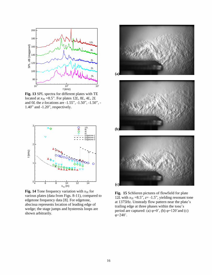
The variation of phase with streamwise distance was measured with the pressure transducer, using the microphone
signal as reference, and the data are shown in Fig. 16(a). These data are taken at the center span (y=0) for four
values of z, as indicated in the legend. For negative z locations (closer to the plate) the data are obtained starting
from the exit of the nozzle. For positive z-locations the data could not be obtained all the way to the nozzle exit
because of constraints from the probe support mechanism. It can be seen that the phase variations for either the
upper or the lower pair of traverses are similar but there is a consistent difference between the two pairs. Average
phase velocities of 0.56Uj and 0.52Uj are estimated from the upper and lower pairs of curves, respectively.
Amplitude variations corresponding to the data of Fig. 16(a) are shown in Fig. 16(b). The transducer essentially
sensed instantaneous total pressure. As stated in §2 there was some uncertainty in the calibration of the probe and
thus these amplitudes are shown simply as measured in rms millivolts. The estimated calibration is 1.1 mv(r.m.s.) =
124 dB (or 0.0046 psi). The amplitude data exhibit the characteristics of an instability wave – initially growing,
saturating to a peak and then decaying. The phase and amplitude variations in the transverse (z) direction,
measured just downstream of the TE of the plate are shown in Fig. 17. The phase variation exhibits a 180 degree
jump across the center plane of the jet. The amplitude drops at this location, grows and then decays in either
direction of z. These data are consistent with a flapping motion of the jet column as seen in the schlieren pictures.
The schlieren pictures showed the structure of the flow field on the x-z cross-sectional plane. Phase-averaged flow
field data were acquired to examine the corresponding unsteady characteristics on the transverse (y-z) plane. These
data were acquired by traversing the pressure transducer on the y-z plane just downstream of the plate’s trailing
edge (x=9”), for 19 phases within the period. Data for four phases are shown in Figs. 18(b)-(e), as examples.
Corresponding time-averaged data are shown at the top in Fig. 18(a). (The reference φ=0 for these data and the
pictures in Fig. 15 were assigned arbitrarily and there is no correspondence). Estimated values of Mach number
normalized by the jet Mach number Mj are plotted. The jet cross section is seen to go through contortions and the

8
unsteady motion is not simply an up-and-down flapping of the jet column against the plate. It is also apparent that
assumption of two-dimensionality for the flow under the resonance may be questionable.
The three-dimensional nature of the flow field is further illustrated by time-averaged Mach number contours
measured at a far downstream location. These data shown in Fig. 19 for the measurement location of x=25.4” (x/D
=12) were acquired with standard Pitot probes. The distribution in Fig. 19(a) represents the same plate
configuration of Figs. 15-18 (plate 12L with xTE=8.5”), yielding the resonant condition. It is clear that an axis switch
has taken place. The major axis of the jet was horizontal at the exit of the nozzle but by the measurement station it
has become vertical. Corresponding data with the plate drawn back are shown in Fig. 19(b). In this case there was
no resonance and the data demonstrate that there was no axis switching. The jet cross section gradually became
round in this case with increase in x. In [7] the evolution of the jet cross section during axis switching is
documented by data at several x-stations, for a different resonant condition with the 12L plate (xTE =12” and z= -
2.12”, Mj =0.99 yielding a resonance at 1100 Hz).
The data in Fig. 19(a) involves a resonance at fp 1375 Hz, corresponding to a Strouhal number (fpD/Uj) of about
0.225 – a value not too far from the ‘preferred mode’ for an equivalent axisymmetric jet. The resonance imposes a
periodic forcing of the jet. Such forcing causes the rectangular jet to go through the axis switching due to the
dynamics of the unsteady azimuthal vortical structures [20]. A periodic forcing causes the sheet of azimuthal
vorticity emanating from the nozzle to roll up into discrete vortex ‘rings’ (with initial shape determined by the
geometry of the nozzle). The non-axisymmetric vortex rings go through self-induced contortions that lead to the
axis switching. The key is the roll-up of the azimuthal vorticity into the nonaxisymmetric rings. This may
sometimes occur naturally, e.g., at low Reynolds numbers when the efflux boundary layer is laminar and
susceptible to naturally occurring disturbances. Periodic perturbations, e.g., by artificial excitation or naturally
occurring phenomena such as screech, also yield the same effect. Without such periodic perturbation the axis
switching is seldom observed at higher jet Reynolds number and Mach number, as is the case in Fig. 19(b). Thus,
the axis switching is likely to be a result rather than the cause for the resonance in the present case. All resonant
tones with jet-surface interaction are expected to result in such axis switching as long as the frequency corresponds
to a Strouhal number not too far from the value noted above.
The unsteady flowfield data presented in this subsection illustrate the enormous effect of the resonance on the
flowfield. The results illustrate that the assumption of two-dimensionality should be viewed with caution in any
analysis of the flow. Furthermore, any numerical simulation must capture the unsteady effects, for otherwise
calculation of even the mean flow field, e.g., captured in Fig. 19(a) will not be possible.
4. Conclusions
An experimental study is conducted to investigate a resonance phenomenon occurring due to the interaction
of a large aspect ratio rectangular jet with a flat plate. The plate is placed parallel to but away from the direct
path of the jet. It is determined that the resonance is not due to structural vibrations of the plate or the support
mechanisms. Effect of parametric variation on the phenomenon is studied. With increasing jet velocity the
resonance is found to ensue at a high subsonic Mach number, become most prominent around transonic
condition and then stop abruptly at low supersonic condition when screech tones begin. It occurs for a range
of transverse (z) positions of the plate relative to the jet. It disappears when the plate is either too far or too
close to the jet. With variation of the z-location of the plate the frequency of the resonance remains
essentially a constant; however, with some plates a ‘stage jump’ to a different frequency is noted. The
frequency increases with increasing jet Mach number and decreasing streamwise distance of the plate’s
trailing edge. Stage jumps are noted with variation of xTE for some plates. Most of the frequency data from
the present experiment are found to be within the bounds of stages 1 and 2 of edgetone phenomenon reported
in the literature. However, within those bounds the data for the different plates vary without any apparent
consistency and a correlation unifying all data could not be inferred. The underlying mechanism of the
resonance appears to have similarity with that of edgetone but remains unclear. Under the resonant condition
the jet cross-section goes through an ‘axis-switching’ and flow visualization indicates a periodic flapping

9
motion of the jet column. The details of the unsteady characteristics of the flowfield for a specific case of the
resonance are documented.
Acknowledgement:
Special thanks are due to Dr. James Bridges for supporting the work as one of the Project managers and also taking
an active interest throughout the study. Thanks are also due to Drs. Stewart Leib and Brenda Henderson for helpful
inputs. Support from the ‘Fixed Wing’ and ‘High Speed’ Projects of NASA’s Fundamental Aeronautics Program is
gratefully acknowledged.
References:
[1] Bridges, J.E., “Noise of embedded high-aspect ratio nozzles”, presented at the NASA Fundamental
Aeronautics Program 2011 Technical Conference, Cleveland, OH, March 15-17, 2011.
[2] Balsa, T.F., Gliebe, R.R., Kantola, R.A., Mani, R., Stringas, E.J. and Wang, J.C.F., “High velocity jet
noise source location and reduction, Task 2 – theoretical developments and basic experiments”, Report No.
FAA-RD-76-79, II, General Electric Co., Aircraft Engine Group, Cincinnatti, OH, May, 1978.
[3] Massey, K.C., Ahuja, K.K. and Gaeta, R., “Noise scaling for unheated low aspect ratio rectangular jets”,
AIAA paper 2004-2946, 10th AIAA/CEAS Aeroacoustics Conference, Manchester, UK 10-12 May 2004.
[4] Brown, C. A., “Jet-surface interaction test: far-field noise results”, Proc. ASME Turbo Expo 2012,
GT2012, Copenhagen, Denmark, June 15-19, 2011.
[5] Afsar, M., Goldstein, M.E. & Leib. S. J., “Prediction of low-frequency trailing edge noise using rapid
distortion theory”, 14th European Turbulence Conference, Lyon, France, Sept 1-4, 2013.
[6] Goldstein, M.E., Afsar, M.Z. and Leib, S.J., “Non-homogeneous rapid distortion theory on transversely
sheared mean flows”, J. Fluid Mech., 2013, (to appear).
[7] Zaman, K.B.M.Q., Brown, C.A. and Bridges, J.E., “Interaction of a rectangular jet with a flat-plate placed
parallel to the flow”, NASA/TM-2013-217879 (E-18684), 2013.
[8] Brown, G.B., “The vortex motion causing edge tones”, Proc. Phys. Soc. (London), 49, pp. 493-507, 1937.
[9] Powell, A., “On the edgetone”, J. Acoust. Soc. of America, vol. 33, pp. 395-409, 1961.
[10] Holger, D.K., Wilson, T.A. and Beavers, G.S., “Fluid mechanics of the edgetone”, J. Acoust. Soc. of America,
62, issue 5, pp. 1116-1128, 1977.
[11] Zaman, K.B.M.Q., "Flow-field surveys for rectangular nozzles”, NASA TM-2012-217410 (see also AIAA
Paper 2012-0069), 2012.
[12] Frate, F.C. and Bridges, J.E., “Extensible rectangular nozzle model system”, AIAA Paper 2011-975, 49th
Aerospace Sciences Meeting, Orlando, Fl, 4-7 January, 2011.
[13] Weinstein, L.M., “Review and update of lens and grid schlieren and motion camera schlieren”, Eur.
Phys. J. Special Topics, 182, pp. 65–95, 2010.
[14] Rockwell, D. and Naudascher, E., “Self-sustained oscillations of impinging shear layers”, Ann. Rev. of
Fluid Mech., vol. 11, pp. 67-93, 1979.
[15] Tam, C.K.W., “Supersonic jet noise”, Ann. Rev. of Fluid Mech., 27, pp. 17-43, 1995.
[16] Bridges, J.E., “Noise from aft deck exhaust nozzles – differences in experimental embodiments”, AIAA
Paper 2014-xxxx, 52nd
Aerospace Sciences Meeting, SciTech-2014, National Harbor, MD, 2014.
[17] Brown, C.A., “Developing an empirical model for jet-surface interaction noise”, AIAA Paper 2014-xxxx,
52nd
Aerospace Sciences Meeting, SciTech-2014, National Harbor, MD, 2014.
[18] Tam, C.K.W. and Yu, J.C., “Trailing edge noise”, AIAA Paper 75-489, 2nd
Aero-acoustics conference,
Hampton, VA, 1975.
[19] Olsen, W. and Boldman, D., “Trailing edge noise data with comparison to theory”, AIAA Paper 79-
1524, 12th Fluid and Plasma Dynamics Conference, Williamsburg, VA, 1979.
[20] Zaman, K.B.M.Q., "Axis switching and spreading of an asymmetric jet: the role of coherent structure
dynamics", J. Fluid Mech., 316, pp. 1-27, 1996.

10
(a)
(b)
(c)
Fig. 1 Experimental facility. (a) setup with
various components marked as follows. 1: Nozzle
(R8); 2: plate; 3-5: mounting posts; 6,7:
breadboards; 8,9: supports; 10: focused schlieren
unit. (b) schematic of setup with co-ordinates. (c)
‘0L’ plate case (vertical knife-edge)
(a)
(b)
Fig. 2 SPL spectra for plate 8L at three jet Mach
numbers (Mj). (a) Data for different rigidity of plate
mounting structure, (b) data for plates of different
material.
f (kHz)
SP
L,d
B(s
tag
gere
d)
10-1
100
101
60
80
100
120
140
160
180
200
Mj= 1.03
0.83
0.67
Red = Bakelite plateBlue = Aluminum plate
f (kHz)
SP
L,d
B(s
tag
gere
d)
10-1
100
101
60
80
100
120
140
160
180
200
Mj= 1.03
0.83
0.67
Red = plate mount 2Blue = plate mount 4

11
(a)
(b)
Fig. 3 SPL spectra for varying z-location of plate;
xTE = 8.5” and Mj =0.96. (a) Plate 12L, (b) Plate 8L.
(a)
(b)
Fig. 4 Overall sound pressure level for varying z-
location of plate; Mj =0.96. (a) xTE =8.5”, (b) xTE =
12.0”.
z (in)
OA
SP
L(d
B)
-3 -2 -1105
110
115
120
0L
2L
8L
12L
z (in)
OA
SP
L(d
B)
-3 -2 -1105
110
115
120
125
130
2L
4L
8L
12L
f (kHz)
SP
L,d
B(s
tag
gere
d)
10-1
100
101
80
100
120
140
160
180
200
-1.00
z = -2.20 in
-1.20
-1.35
-1.50
-1.65
-1.80
-2.0
f (kHz)
SP
L,d
B(s
tag
gere
d)
10-1
100
101
90
120
150
180
-1.45
-1.50
-1.55
-1.65
-1.75
z=-1.95 in

12
(a)
(b)
(c)
Fig. 5 Schlieren pictures of flowfield for varying
z-location of plate 8L; xTE =8.5”, Mj = 0.96. (a) z=
-1.0”, (b) z= -1.35” and (c) z= -2.2”.
(a)
f (kHz)
SP
L,d
B(s
tag
gere
d)
10-1
100
101
60
90
120
150
180
210M
j= 1.06
1.03
0.99
0.93
0.83
0.77
0.67
0.56
0
(b)
Fig. 6 Data for plate 12L at different Mj; xTE =8.5”,
z= -1.5”. (a) SPL spectra, (circled peak at Mj =1.06
is due to screech), (b) tone frequency with scale on
right, and OASPL and tone amplitude (SPL at fp)
with scale on left.
Mj
am
plit
ud
e(d
B)
f p(k
Hz)
0.6 0.7 0.8 0.9 1 1.190
100
110
120
130
140
<= OASPL
<= SPL at fp
tone frequency =>
1.2
1.3
1.4

13
(a)
(b)
(c)
Fig. 7 Schlieren pictures of flowfield for plate
12L at three Mj; xTE =8.5”, z= -1.5”. (a) Mj =0.83,
(b) Mj =0.99 and (c) Mj =1.06.
(a) f (kHz)
SP
L,d
B(s
tag
gere
d)
10-1
100
101
90
120
150
180
210
xTE
= 13 in
12
11
10
9
8
7
6
(b)
Fig. 8 Data for plate 12L with varying xTE at Mj=
0.96. (a) SPL spectra, (b) tone frequency (scale on
right) and amplitudes (scale on left).
xTE
(in)
am
plit
ud
e(d
B)
f p(k
Hz)
6 8 10 12 14
100
120
140
0.5
1
1.5
2
<= OASPL
Tone Frequency =>
<= SPL at fp

14
(a) f (kHz)
SP
L,d
B(s
tag
gere
d)
10-1
100
101
90
120
150
180
210
xTE
= 13 in
12
11
10
9
8
7
6
(b)
Fig. 9 Data for plate 8L with varying xTE at Mj=
0.96. (a) SPL spectra, (b) tone frequency (scale on
right) and amplitudes (scale on left).
(a) f (kHz)
SP
L,d
B(s
tag
gere
d)
10-1
100
101
90
120
150
180
210
xTE
= 13 in
12
11
10
9
8
7
6
(b)
Fig. 10 Data for plate 4L with varying xTE at Mj=
0.96. (a) SPL spectra, (b) tone frequency (scale on
right) and amplitudes (scale on left).
xTE
(in)
am
plit
ud
e(d
B)
f p(k
Hz)
6 8 10 12 14
100
120
140
1
2
3
<= OASPL
Tone Frequency =>
<= SPL at fp
xTE
(in)
am
plit
ud
e(d
B)
f p(k
Hz)
6 8 10 12 14
100
120
140
0.5
1
1.5
2
<= OASPL
Tone Frequency =>
<= SPL at fp

15
(a) f (kHz)
SP
L,d
B(s
tag
gere
d)
10-1
100
101
90
120
150
180
210
xTE
= 13 in
12
11
10
9
8
7
6
(b)x
TE(in)
am
plit
ud
e(d
B)
f p(k
Hz)
6.5 8.5 10.5 12.5 14.5
100
120
140 1
2
3
<= OASPL
Tone Frequency =>
<= SPL at fp
Fig. 11 Data for 0L case with varying xTE at Mj=
0.96. (a) SPL spectra, (b) tone frequency (scale on
right) and amplitudes (scale on left).
(a)
(b)
(c)
Fig. 12 Schlieren pictures of flowfield for the 0L
case at three different Mj; xTE =8.5”, z= -1.2”. (a)
Mj =0.67, (b) Mj =0.96 and (c) Mj =1.03.
16
Fig. 13 SPL spectra for different plates with TE
located at xTE =8.5”. For plates 12L, 8L, 4L, 2L
and 0L the z-locations are -1.55”, -1.50”, -1.50”, -
1.40” and -1.20”, respectively.
xTE
(in)
f(k
Hz)
4 6 8 10 12 140
1
2
312L8L4L0LEdgetone-1Edgetone-2Edgetone-3
>
>
>
<
Fig. 14 Tone frequency variation with xTE for
various plates (data from Figs. 8-11), compared to
edgetone frequency data [8]. For edgetone,
abscissa represents location of leading edge of
wedge; the stage jumps and hysteresis loops are
shown arbitrarily.
(a)
(b)
(c)
Fig. 15 Schlieren pictures of flowfield for plate
12L with xTE =8.5”, z= -1.5”, yielding resonant tone
at 1375Hz. Unsteady flow pattern near the plate’s
trailing edge at three phases within the tone’s
period are captured: (a) φ=0˚, (b) φ=120˚and (c)
φ=240˚.
f (kHz)
SP
L,d
B(s
tag
gere
d)
10-1
100
101
80
100
120
140
160
180
200
12L
8L
4L
2L
0L
17
(a)
(b)
Fig. 16 Streamwise variation of phase and
amplitude of the tone fundamental for the same
case of Fig. 15. Data are for four transverse (z)
locations as indicated (y=0). (a) Phase variation, (b)
amplitude (r.m.s. of pressure fluctuation) variation.
Data obtained by spectral analysis of signal from
pressure transducer relative to 60˚ microphone
signal.
Fig. 17 Phase and amplitude variation for the
resonance case of Figs. 15 and 16 in the transverse
(z) direction, downstream of plate’s trailing edge
(x=9”, y=0).
z (in)
p'(a
rbitra
ryscale
)
(d
eg
)
-2 -1 0 1 2
102
103
104
90
-180
0
-90
Platelocation
=>
<=
x (in)
p'(a
rbitra
ryscale
)
0 5 10 1510
0
101
102
z = -1.21
z = -0.5
z = +0.5
z = +1.21
x (in)
ph
ase
(deg
)
0 5 10 150
360
720
1080z = -1.21
z = -0.5
z = +0.5
z = +1.21

18
(a)
(b)
(c)
(d)
(e)
Fig. 18 Cross-sectional distribution of M/Mj for
plate 12L at x=9” for the resonant condition of Figs.
15-17. Time-averaged data shown in (a); (b), (c),
(d) and (e) show phase-averaged data at four phases
as indicated.
(a)
(b)
Fig. 19 Time-averaged M/Mj contours measured at
x=25.4” for a resonant and a non-resonant condition
with plate 12L. (a) xTE =8.5”, z= -1.5”, Mj =0.96; (b)
xTE =3”, z= -2.5”, Mj =0.96 (plate drawn back, no
resonance). Data obtained by standard Pitot probe
surveys.