Embed Size (px)
Citation preview

Available athttp://pvamu.edu/aam
Appl. Appl. Math.ISSN: 1932-9466
Applications and Applied
Mathematics:
An International Journal(AAM)
Vol. 14, Issue 1 (June 2019), pp. 416–436
Resonance in the Motion of a Geocentric Satellite Due toPoynting-Robertson Drag and Equatorial Ellipticity of the Earth
1Charanpreet Kaur, 2Binay Kumar Sharma and 3Sushil Yadav
1Department of MathematicsS.G.T.B. Khalsa College
University of DelhiDelhi, India
2Department of MathematicsS.B.S. College
University of DelhiDelhi, India
3Department of MathematicsMaharaja Agrasen College
University of DelhiDelhi, India
Received: April 20, 2018; Accepted: November 6, 2018
Abstract
In this paper, the problem of resonance in a motion of a geocentric satellite is numerically investi-gated under the consolidated gravitational forces of the Sun, the Earth including Earth’s equatorialellipticity parameter and Poynting-Robertson (P-R) drag. We are presuming that bodies lying onan ecliptic plane are the Sun and the Earth, and satellite on orbital plane. Resonance is monitoredbetween satellite’s mean motion and average angular velocity of the Earth around the Sun, and alsobetween satellite’s mean motion and equatorial ellipticity parameter of the Earth. We also performa systematic and thorough analysis in an attempt to understand the effect of Earth’s equatorial el-lipticity parameter and P-R drag on time period and amplitude of oscillations at different criticalpoints.
416

AAM: Intern. J., Vol. 14, Issue 1 (June 2019) 417
Keywords: Three-body problem; Ecliptic Plane; Resonance; Poynting-Robertson drag
MSC 2010 No.: 37M10, 37M05, 70F07, 34C60
1. Introduction
The Poynting-Robertson is a process by which, a dust grain orbiting a star loses its angular mo-mentum relative to its orbit around the star due to solar radiation. This is related to radiationpressure tangential to the grain’s motion. This causes dust that is small enough to be affected bythis drag, but too large to be blown away from the star by radiation pressure, to spiral slowly intothe star. In celestial mechanics, general three-body problem is the problem of taking initial set ofquantities (positions, masses and velocities) of the three bodies for some particular point in timeand then determining their motions, in accordance with Newton’s laws of motion and universalgravitation. It’s a special case of the general n-body problem. Three-body problem has been stud-ied by many authors. Poynting (1903) and Robertson (1937) discussed the radiation pressure, theDoppler shift of incident radiation and P-R drag. The radiating body generally radiates force onthe particle which constitutes three terms i.e. the incident radiation, the radiation pressure and theDoppler shift.The force caused by absorption and successive re-emission of radiation comprise P-R effect. The motion of an artificial satellite due to radiation pressure of the Sun has been studiedby Brouwer (1963).
Bhatnagar and Mehra (1986) examined the motion of a satellite by taking the gravitational forcesof the the moon, the Earth and the Sun (with radiation pressure). Ragos and Zafiropoulos (1995)have numerically studied the existence and stability of equilibrium points for particles moving inthe vicinity of two massive bodies which exert light radiation pressure. Resonance behaviour in thespin-orbit coupling in celestial mechanics in a conservative field has been discussed by Celletti andChierchia (2000). They have studied the periodic-orbit by using symplectic mapping. Callegari andYokoyama (2001) showed that a satellite beginning with a nearly circular orbit experienced hugeeccentricity variations relying on the initial angle of the orbit to the reference plane. Secondly, byincluding gravitational effect of the Moon, they found two regions with huge variations of eccen-tricity. Thus, in both cases they found huge regions of the phase space where stability (large-term)of imaginary Earth’s satellite is impossible. Long term evolution of more than 54 years, of objectsreleased in geostationary orbit with upto 50m2/kg area-mass ratio was examined by Pardini andAnselmo (2008), by acknowledging geopotential harmonics, eclipses with direct solar radiationpressure, lunar solar perturbations and air drag (when applicable). They also concluded that evolu-tion of eccentricity is influenced by annual oscillations with smaller large period modulations.
Non gravitational forces, dissipative forces (linear Stokes, P-R drag) play a prominent role in solarsystem. P-R effect is one of the most important mechanism of dissipation. Under different kindsof dissipative forces, Celletti and Stefanelli (2011) have discussed the dynamics of CR3BP. Theyshowed that semi major axis decrease often due to dissipation and consequently the collision takesplace between one of the primaries and minor bodies. Quarles et al. (2012) has studied the reso-nances for co-planar circular R3BP for the mass ratio between 0.10 and 0.50 and used the methodof maximum Lyaponov exponent to locate the resonances. To classify the periodicity and to de-

418 C. Kaur et al.
termine the kind of resonance Fast Fourier Transform was used. They showed that for high valuesof resonance, orbital stability is ensured where single resonance is present. Yadav and Aggarwal(2013a) have studied the resonance in a geo-centric satellite including it’s equatorial ellipticity.They graphically showed that amplitude and time-period decrease when equatorial ellipticity pa-rameter increases from 00 to 450. Detailed description of the perturbation theory to determine thelocation of resonance based on approximations to a harmonic oscillations have been discussed byRosemary (2013). Hary (2014) has discussed the prediction of satellite motion under the gravita-tional effects of the Earth and radiation pressure by Sun in terms of KS symmetrical variables.
Numerous authors have discussed the P-R effect in the three body problem on numerical exper-iments by taking any two of three (1)Three-body problem (2) Resonance (3) P-R drag. We haveattempted to solve the problem by taking all the three factors mentioned above. New parameter,Earth’s equatorial ellipticity is added to our previous work where resonance is observed in threedifferent parameters instead of two.
Thorough study of equations of motion in Section 2 of this paper shows that resonance occursat five critical points Ri’s, i = 1 − 5 in the motion of the satellite between the satellite’s meanmotion (n) and the average angular velocity of the Earth around the Sun (δ0). The focus of thispaper is to find the resonance in the motion of geo-centric satellite due to P-R drag and Earth’sequatorial ellipticity parameter (Γ) in the three-body problem if regression angle is constant. Ifregression angle is not constant then resonance between n and Γ occurs at the same four pointsR′i’s, i = 1− 4. Apart from this, resonance occurs at many points with three frequencies betweenn, δ0 and Γ. Evaluation of the corresponding amplitudes and time periods at resonance points havebeen illustrated in Section 3. Discussions and conclusions are given in Section 4, in which wehave compared the amplitude and time-period at same resonant point for different values of solarradiation parameter. We have also discussed the variation in the amplitudes and time periods atresonant points 1 : 1 and 1 : 2 with P-R drag and without P-R drag. Furthermore, amplitudes andtime-periods due to Earth’s equatorial ellipticity parameter at different resonant points have alsobeen examined.
2. Statement of the problem, Equations of motion and resonance
Let x, y, z be the co-ordinate system of satellite (S) with the center of the Earth (E) as originwith unit vectors ˆi, ˆj and ˆk along the co-ordinates axes respectively. Let x, y and z be another setof co-ordinate system in the same plane, with the center of the Earth as origin, and unit vectorsi, j and k along the co-ordinate axes. Let X , Y and Z with unit vectors I , J and K along theco-ordinate axes be geo-centric reference system, while the XY plane is the Earth’s equatorialplane. Let MS , MS and ME represent the masses of the Sun, Earth and satellite respectively. Thesatellite moves around the Earth in orbital plane. Let the satellite be revolving around the Earthwith angular velocity ~ω and the system is also revolving with the same angular velocity ~ω. It isassumed that the ecliptic plane is the reference plane and the satellite’s orbital plane is fixed. Let~rE , ~rs and ~r represent the vectors from Sun and Earth, Sun and satellite and Earth and satelliterespectively; χ be the vernal equinox, α the angle between ecliptic plane and orbital plane, β theangle between direction of satellite and the direction of the ascending node, δ the orbital angle of

AAM: Intern. J., Vol. 14, Issue 1 (June 2019) 419
the Earth around the Sun, γ be the satellite orbital regression angle, ε∗ be the angle between eclipticplane and equatorial plane (obliquity), c∗ the velocity of light and ~βE spin of the Earth.
Figure 1. Configuration of the three body problem with co-ordinate axis
(a) (b)
Figure 2. (a) Configuration of the three body problem in vector form (b) Coordinate system of the Satellite in(XG, YG, ZG) system
2.1. Equations of motion in polar form
Let ~FS be the Poynting-Robertson drag per unit mass acting on the satellite due to radiating body(Sun) as shown in the Figure 2a, given by (Ragos and Zafiropoulos (1995))
MS~FS = ~g1 + ~g2 + ~g3,
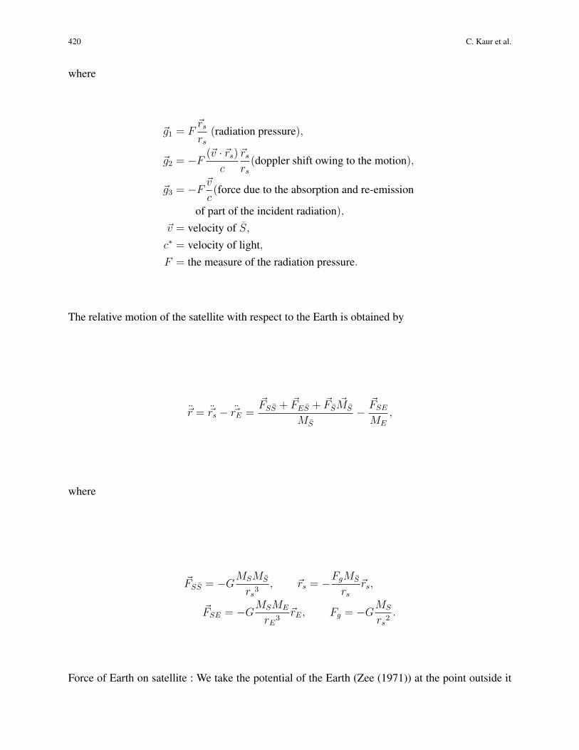
420 C. Kaur et al.
where
~g1 = F~rsrs
(radiation pressure),
~g2 = −F (~v · ~rs)c
~rsrs
(doppler shift owing to the motion),
~g3 = −F ~vc
(force due to the absorption and re-emission
of part of the incident radiation),
~v = velocity of S,c∗ = velocity of light,F = the measure of the radiation pressure.
The relative motion of the satellite with respect to the Earth is obtained by
~r = ~rs − ~rE =~FSS + ~FES + ~FS
~MS
MS
−~FSE
ME
,
where
~FSS = −GMSMS
rs3, ~rs = −FgMS
rs~rs,
~FSE = −GMSME
rE3~rE, Fg = −GMS
rs2.
Force of Earth on satellite : We take the potential of the Earth (Zee (1971)) at the point outside it

AAM: Intern. J., Vol. 14, Issue 1 (June 2019) 421
in the form
U =GMEMS
r
{1−
J2R2⊕
2r2
(3Z2
r2− 1
)}− 3
J22R
2⊕
r2cos2 δ∗ cos 2Γ + ...,
~FES =∂U
∂r~r +
∂U
∂XI +
∂U
∂YJ +
∂U
∂ZK
= −GMEMS
r3
(1−
3J2R2⊕
2r2(5Z2
r2− 1)− 15J2
2R⊕2
r4{(r · I)2
+ (r · J)2} cos 2Γ
)~r +
6J22R⊕
2
r2{(r · I)I + (r · J)J} cos 2Γ
+6J2
2R⊕2
r2{(r · J)I − (r · I)J} sin 2Γ +
3J2R2⊕
r2ZK,
G = Gravitational constant,β′ = ∠χES ′ = angle between the projection of the line ES in the
plane of the equator (ES ′) and the vernal equinox Figure 2b,βE = angle between the vernal equinox and minor axis of
the Earth’sequatorial section Figure 2b,J2 = coefficient due to the oblateness of the Earth,R⊕ = mean radius of the Earth,J2
2 = coefficient due to the Earth’s equatorial ellipticity,Γ = angle measured from the major axis of the Earth’s
equatorial ellipse to the satellite,δ∗ = declination of the satellite.
Thus,
~r = −qFg~rsrs− GME
r3
{(1−
3J2R2⊕
2r2(5Z2
r2− 1)
− 15J22R⊕
2
r4{(r · I)2 + (r · J)2} cos 2Γ
)~r
+6J2
2R⊕2
r2{(r · I)I + (r · J)J} cos 2Γ
+6J2
2R⊕2
r2{(r · J)I − (r · I)J} sin 2Γ
+3J2(R⊕)2
r2ZK
}+GMs
r3E
~rE − pFg
((~v · ~rs)~rscrs
+~v
c
),
where q = 1−F/Fg exhibit the relation between the gravitational force and the radiation pressureresulting from the Sun. Evidently 0 < q < 1 and p = 1− q. Motion of the Earth relative to the sun

422 C. Kaur et al.
is given by
δ2 =GMs
r3E
,
also
~r = rˆi, ~rE = rE rE, rE = cos δi+ sin δj,
~rE = rE cos δi+ rE sin δj.
Using these values in the equation of motion of the satellite with respect to the Earth in vector formcan be written as
~r = −qGMs~rsr3s
− GME
r3
{(1−
3J2R2⊕
2r2(5Z2
r2− 1)− 15J2
2R⊕2
r2{(i · I)2
)ri
+ (i · J)2} cos 2Γri+6J2
2R⊕2
r{(i · I)I + (i · J)J} cos 2Γ
+6J2
2R⊕2
r{(i · J)I − (i · I)J} sin 2Γ +
3J2(R⊕)2
r2ZK
}+GMs
r3E
~rE
+ δ2rE(cos δi+ sin δj)− pFg
{(~v · ~rs)~rs
crs+~v
c
}. (1)
In the rotating frame of reference with angular velocity ~ω of the satellite about the center of theEarth, we have
~r =d2r
dt2ˆi+ 2
dr
dt
(~ω × ˆi
)+ r
(d~ω
dt× ˆi
)+ r{(~ω · ˆi)~ω − (~ω · ~ω)i}, (2)
where
~ω = β ˆk + γk.
Taking dot products of Equations (1) and (2) with ˆi and ˆj respectively, and equating the respec-tive coefficients, we get the equations of motion of the satellite in the synodic coordinate system

AAM: Intern. J., Vol. 14, Issue 1 (June 2019) 423
(Bhatnagar and Mehra (1986))
d2r
dt2− rβ2 +
GME
r2
= −qGMs(~rs · ˆi)r3s
+ δ2rE{cos β cos(δ − γ) + cosα sin β sin(δ − γ)}
−3GMEJ2R
2⊕[1− 3(i.K)2]
2r4+
9GMEJ22R⊕
2
r4{(i · I)2 + (i · J)2}
× cos 2Γ− 6GMEJ22R⊕
2
r{(i · J)(I · ˆi)− (i · I)(J · ˆi)} sin 2Γ
− pGMs
r2s
{(~v · ~rs)(~rs · ˆi)
crs+
(~v · ˆi)c
}, (3)
d(r2β)
dt= −δ2rrE {sin β cos(δ − γ)− cosα cos β sin(δ − γ)}
− qGMsr(~rs · ˆj)r3s
−3GMEJ2R
2⊕ (i.K)(ˆj.K)
2r3
− 6J22R⊕
2
r{(i · I)(I · ˆj) + (i · J)(J · ˆj)} cos 2Γ
− 6J22R⊕
2
r{(i · J)(I · ˆj)− (i · I)(J · ˆj)} sin 2Γ
− pGMs
r2s
{(~v · ~rs)(~rs · ˆj)
crs+
(~v · ˆj)c
}. (4)
Table 1. Relation between coordinate system
i j k
I 1 0 0
J 0 cos ε sin ε
K 0 − sin ε cos ε
i j kˆi a1 b1 c1
ˆj a2 b2 c2
ˆk a3 b3 c3
where
a1 = cos β cos γ − cosα sin β sin γ, a2 = − sin β cos γ − cosα cos β sin γ,
a3 = sinα sin γ, b1 = cos β sin γ − cosα sin β cos γ,
b2 = − sin β sin γ + cosα cos β cos γ, b3 = cos γ sinα,
c1 = sinα sin β, c2 = sinα cos β, c3 = cosα.
Equations (3) and (4) are the required equations of motion of the satellite in polar form. Theseequations are not integrable, therefore we follow the perturbation technique and replace r, β and γby their steady state values r0, β0, γ0 and we may take β = β0t, γ = γ0t and δ = δt respectively.

424 C. Kaur et al.
Putting the steady state values in the R.H.S of Equations (3) and (4), we get
d2r
dt2− rβ2 +
GME
r2
= −qGMs(~rs · ˆi)r3s
−3GMEJ2R
2⊕{1− 3(i.K)2}2r4
0
+ δ2rE{cos β0t cos(δ − γ0)t+ cosα sin β0t sin(δ − γ0)t)}
+9GMEJ
22R⊕
2
r4{(i · I)2 + (i · J)2} cos 2Γ
− pGMs
r2s
{(~v · ~rs)(~rs · ˆi)
crs+
(~v · ˆi)c
}, (5)
d(r2β)
dt= −qGMsr0
(~rs · ˆj)r3s
−3GMEJ2R
2⊕ (i.K)(ˆj.K)
2r30
− δ2r0rE{sin β0t cos(δ − γ0)t+ cosα cos β0t sin(δ − γ0)t}
− 6J22R⊕
2
r0
{(i · I)(I · ˆj) + (i · J)(J · ˆj)} cos 2Γ
− 6J22R⊕
2
r0
{(i · J)(I · ˆj)− (i · I)(J · ˆj)} sin 2Γ
− pr0GMs
r2s
{(~v · ~rs)(~rs · ˆj)
crs+
(~v · ˆj)c
}. (6)
Now,
~v = {−rE(δ − γ0) cos β0t sin(δ − γ0)t+ rE(δ − γ0) cosα sin β0t
cos(δ − γ0)t}i+ {r0β0 + rE(δ − γ0) sin β0t sin(δ − γ0)t
+ rE(δ − γ0) cos β0t cos(δ − γ0)t cosα}ˆj
− {rE(δ − γ0) sinα cos(δ − γ0)t}ˆk,K = − sin ε∗j + cos ε∗k
= − sin ε∗ (ib1 + ˆjb2 + ˆkb3) + cos ε∗(c1ˆi+ c2
ˆj + c3ˆk)
= (−b1 sin ε∗ + c1 cos ε∗ )i+ (−b2 sin ε∗ + c2 cos ε∗)ˆj
+ (−b3 sin ε∗ + c3 cos ε∗)ˆk.
With the help of above values, transformations in Tables 1 and taking r2β = constant = h, r = 1u
,

AAM: Intern. J., Vol. 14, Issue 1 (June 2019) 425
we get
d2u
dβ2+ u =
GME
h2+ qGMs
~rs · ˆir3sh
2u2+
3GMEJ2(R0)2u2{1− 3(i.K)2}2h2
− δ2
h2u2{cos β0t cos(δ − γ0)t+ cosα sin β0t sin(δ − γ0)t}
− 9GMEJ22R⊕
2u2
h2{(i · I)2 + (i · J)2} cos 2Γ
+ pGMs
r2sh
2u2
{(~v · ~rs)(~rs · ˆi)
crs+
(~v · ˆi)c
}. (7)
The solution of unperturbed system
d2u
dβ2+ u =
GME
r40β0
2 ,
is given by
l
r= 1 + e cos(β − ω1),
where
l = a(1− e2),
u =1 + e cos(β − ω1)
a(1− e2),
e, ω1 = constants of integration.
Let us consider
β − ω1 = f = β0t = nt(say).
Since e < 1, we have
(1 + e cosnt)h1 ≈ 1 + h1e cosnt,
we are ignoring terms due to oblateness J2 of the Earth in this paper, since we are investigating the
426 C. Kaur et al.
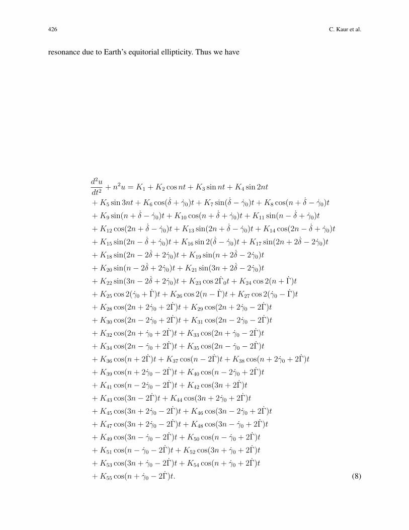
resonance due to Earth’s equitorial ellipticity. Thus we have
d2u
dt2+ n2u = K1 +K2 cosnt+K3 sinnt+K4 sin 2nt
+K5 sin 3nt+K6 cos(δ + γ0)t+K7 sin(δ − γ0)t+K8 cos(n+ δ − γ0)t
+K9 sin(n+ δ − γ0)t+K10 cos(n+ δ + γ0)t+K11 sin(n− δ + γ0)t
+K12 cos(2n+ δ − γ0)t+K13 sin(2n+ δ − γ0)t+K14 cos(2n− δ + γ0)t
+K15 sin(2n− δ + γ0)t+K16 sin 2(δ − γ0)t+K17 sin(2n+ 2δ − 2γ0)t
+K18 sin(2n− 2δ + 2γ0)t+K19 sin(n+ 2δ − 2γ0)t
+K20 sin(n− 2δ + 2γ0)t+K21 sin(3n+ 2δ − 2γ0)t
+K22 sin(3n− 2δ + 2γ0)t+K23 cos 2Γ0t+K24 cos 2(n+ Γ)t
+K25 cos 2(γ0 + Γ)t+K26 cos 2(n− Γ)t+K27 cos 2(γ0 − Γ)t
+K28 cos(2n+ 2γ0 + 2Γ)t+K29 cos(2n+ 2γ0 − 2Γ)t
+K30 cos(2n− 2γ0 + 2Γ)t+K31 cos(2n− 2γ0 − 2Γ)t
+K32 cos(2n+ γ0 + 2Γ)t+K33 cos(2n+ γ0 − 2Γ)t
+K34 cos(2n− γ0 + 2Γ)t+K35 cos(2n− γ0 − 2Γ)t
+K36 cos(n+ 2Γ)t+K37 cos(n− 2Γ)t+K38 cos(n+ 2γ0 + 2Γ)t
+K39 cos(n+ 2γ0 − 2Γ)t+K40 cos(n− 2γ0 + 2Γ)t
+K41 cos(n− 2γ0 − 2Γ)t+K42 cos(3n+ 2Γ)t
+K43 cos(3n− 2Γ)t+K44 cos(3n+ 2γ0 + 2Γ)t
+K45 cos(3n+ 2γ0 − 2Γ)t+K46 cos(3n− 2γ0 + 2Γ)t
+K47 cos(3n+ 2γ0 − 2Γ)t+K48 cos(3n− γ0 + 2Γ)t
+K49 cos(3n− γ0 − 2Γ)t+K50 cos(n− γ0 + 2Γ)t
+K51 cos(n− γ0 − 2Γ)t+K52 cos(3n+ γ0 + 2Γ)t
+K53 cos(3n+ γ0 − 2Γ)t+K54 cos(n+ γ0 + 2Γ)t
+K55 cos(n+ γ0 − 2Γ)t. (8)

AAM: Intern. J., Vol. 14, Issue 1 (June 2019) 427
The solution is given by
u = A cos(nt− ε∗1) +K1
n2− K2t sinnt
2n+K3t cosnt
2n+K4 sin 2nt
n2 − 4(n)2
+K5 sin 3nt
n2 − (3n)2+
K6(δ − γ0)t
n2 − (δ − γ0)2+K7 sin(δ − γ0)t
n2 − (δ − γ0)2
+K8 cos(n+ δ − γ0)t
n2 − (n+ δ − γ0)2+K9 sin(n+ δ − γ0)t
n2 − (n+ δ − γ0)2+K10 cos(n− δ + γ0)t
n2 − (n− δ + γ0)2
+K11 sin(n− δ + γ0)t
n2 − (n− δ + γ0)2+K12 cos(2n+ δ − γ0)t
n2 − (2n+ δ − γ0)2+K13 sin(2n+ δ − γ0)t
n2 − (2n+ δ − γ0)2
+K14 cos(2n− δ + γ0)t
n2 − (2n− δ + γ0)2+K15 sin(2n− δ + γ0)t
n2 − (2n− δ + γ0)2+K16 sin 2(δ − γ0)t
n2 − 4(δ − γ0)2
+K17 sin(2n+ 2δ − 2γ0)t
n2 − (2n+ 2δ − 2γ0)2+K18 sin(2n− 2δ + 2γ0)t
n2 − (2n− 2δ + 2γ0)2
+K19 sin(n+ 2δ − 2γ0)t
n2 − (n+ 2δ − 2γ0)2+K20 sin(n− 2δ + 2γ0)t
n2 − (n− 2δ + 2γ0)2
+K21 sin(3n+ 2δ − 2γ0)t
n2 − (3n+ 2δ − 2γ0)2+K22 sin(3n− 2δ + 2γ0)t
n2 − (3n− 2δ + 2γ0)2
+K23 cos 2Γt
n2 − 4Γ20
+K24 cos 2(n+ Γ)t
n2 − 4(n+ Γ)2+K25 cos 2(γ0 + Γ)t
n2 − 4(γ0 + Γ)2
+K26 cos 2(n− Γ)t
n2 − 4(n− Γ)2+K27 cos 2(γ0 − Γ)t
n2 − 4(γ0 − Γ)2+K28 cos(2n+ 2γ0 + 2Γ)t
n2 − (2n+ 2γ0 + 2Γ)2
+K29 cos(2n+ 2γ0 − 2Γ)t
n2 − (2n+ 2γ0 − 2Γ0)2+K30 cos(2n− 2γ0 + 2Γ)t
n2 − (2n− 2γ0 + 2Γ)2
+K31 cos(2n− 2γ0 − 2Γ)t
n2 − (2n− 2γ0 − 2Γ)2+K32 cos(2n+ γ0 + 2Γ)t
n2 − (2n+ γ0 + 2Γ)2
+K33 cos(2n+ γ0 − 2Γ)t
n2 − (2n+ γ0 − 2Γ)2+K34 cos(2n− γ0 + 2Γ)t
n2 − (2n− γ0 + 2Γ)2
+K35 cos(2n− γ0 − 2Γ)t
n2 − (2n− γ0 − 2Γ)2+K36 cos(n+ 2Γ)t
n2 − (n+ 2Γ)2+K37 cos(n− 2Γ)t
n2 − (n− 2Γ)2
+K38 cos(n+ 2γ0 + 2Γ)t
n2 − (n+ 2γ0 + 2Γ)2+K39 cos(n+ 2γ0 − 2Γ)t
n2 − (n+ 2γ0 − 2Γ)2
+K40 cos(n− 2γ0 + 2Γ)t
n2 − (n− 2γ0 + 2Γ)2+K41 cos(n− 2γ0 − 2Γ)t
n2 − (n− 2γ0 − 2Γ)2
+K42 cos(3n+ 2Γ)t
n2 − (3n+ 2Γ)2+K43 cos(3n− 2Γ)t
n2 − (3n− 2Γ)2+K44 cos(3n+ 2γ0 + 2Γ)t
n2 − (3n+ 2γ0 + 2Γ)2
+K45 cos(3n+ 2γ0 − 2Γ)t
n2 − (3n+ 2γ0 − 2Γ)2+K46 cos(3n− 2γ0 + 2Γ)t
n2 − (3n− 2γ0 + 2Γ)2

428 C. Kaur et al.
+K47 cos(3n− 2γ0 − 2Γ)t
n2 − (3n− 2γ0 − 2Γ)2+K48 cos(3n− γ0 + 2Γ)t
n2 − (3n− γ0 + 2Γ)2
+K49 cos(3n− γ0 − 2Γ)t
n2 − (3n− γ0 − 2Γ)2+K50 cos(n− γ0 + 2Γ)t
n2 − (n− γ0 + 2Γ)2
+K51 cos(n− γ0 − 2Γ)t
n2 − (n− γ0 − 2Γ)2+K52 cos(3n+ γ0 + 2Γ)t
n2 − (3n+ γ0 + 2Γ)2
+K53 cos(3n+ γ0 − 2Γ)t
n2 − (3n+ γ0 − 2Γ)2+K54 cos(n+ γ0 + 2Γ)t
n2 − (n+ γ0 + 2Γ)2
+K55 cos(n+ γ0 − 2Γ)t
n2 − (n+ γ0 − 2Γ)2, (9)
values of constant Ki’s are given in Appendix A (which can be obtained from the authors).
2.2. Resonance
It is understandable now that if any one of the denominators ceases to exit, the motion becomesindefinite in Equation (2.1), and hence the resonance occur at these points, called critical points.It is found that resonance occurs at many points with three frequencies on account of n, δ, γ0 orn, γ0, Γ and at four points (n = Γ), (n = 2Γ), (3n = 2Γ), (2n = Γ) due to equatorial ellipticityparameter of the Earth. Also it is found that resonance occurs at five points (n = δ), (n = 2δ),(3n = δ), (2n = δ), (3n = 2δ) in frequencies n and δ. If we take solar radiation pressure asperturbing force, then there are only three critical points at which resonance occurs. If we considervelocity dependent terms of P-R drag, then five points of resonance occur where two points ofresonance are same, and 1 : 2 and 3 : 2 resonances occur only due to velocity dependent terms ofP-R drag .
3. Time period and amplitude at critical points where resonance occurs
Time period and amplitude at n = 2δ
We have followed the method discussed in Brown and Shook (1933) to determine time period andamplitude at n = 2δ. It is suggested to obtain the solution of Equation.(8) when that of
d2u
dt2+ n2u = 0, (10)
is periodic and is known. The solution of Equation (10) is
u = k cos s,
where
s = nt+ ε∗,
n =k1
k= function of k; (11)

AAM: Intern. J., Vol. 14, Issue 1 (June 2019) 429
k, k1 and ε∗ are arbitrary constants. As we are probing the resonance in the motion of the satelliteat the point n = 2δ, in our case the resulting Equation (8) can be written as
d2u
dt2+ n2u = HA′ cosn′t = Hγ′,
where
H =pFgrE
2δ
4cars(1− e2)= constant, n′ = 2δ,
A′ = − sin2 α,
γ′ =∂γ
∂u= A′ cosn′t, γ = uA′ cosn′t,
γ =A′k
2{cos(n′t+ s) + cos(n′t− s)}. (12)
Then,dk
dt=H
W
∂u
∂sγ′ =
H
W
∂γ
∂s, (13)
ds
dt= n− H
W
∂u
∂kγ′ = n− H
W
∂γ
∂k, (14)
where
W =∂
∂k(n∂u
∂s)∂u
∂s− n∂
2u
∂s2
∂u
∂k= a function of k only.
Since n and W are function of k only, we can put Equations (13) and (14) into canonical form withnew variables defined by,
dk1 = Wdk, (15)dB = −ndk1 = −nWdk, (16)
Equations (15) and (16) can be put in the formdk1
dt=
∂
∂s(B +Hγ),
ds
dt= − ∂
∂s(B +Hγ).
Differentiating Equation (14) with respect to t and substituting the expression for dsdt
and dkdt
, wehave
d2s
dt2=H
W
(∂n
∂k
∂γ
∂s− n ∂2γ
∂s∂k− ∂2γ
∂k∂t
)+H2
K2
(∂2γ
∂s∂k
∂γ
∂k−W ∂
∂k
(1
W
∂γ
∂k
)∂γ
∂s
). (17)
Since the last expression of Equation (17) has the factor H2 it may, in general be neglected in afirst approximation. In Equation(12) we find s and t are present in γ′ as sum of the periodic termswith argument s′ = s− n′t, the affected term in our case is
γ =kA′ cos s′
2. (18)

430 C. Kaur et al.
Equation (17) for s′ is then,
d2s′
dt2+ (n− n′)2 H
W
∂
∂k
(1
n− n′∂γ
∂s′
)= 0 (19)
ord2s′
dt2− (n− n′)2 H
2W
∂
∂k
(kA′
n− n′
)sin s′ = 0. (20)
At first approximation, we put constants
k = k0, n = n0, W = W0.
Then, Equation (20) can be written as
d2s′
dt2− (n− n′)2 H
2W
∂
∂k
(kA′
n− n′
)sin s′ = 0. (21)
If the oscillations be small, then Equation (21) may be put in the form
d2s′
dt2− (n− n′)2 H
2W
∂
∂k
(kA′
n− n′
)s′ = 0
ord2s′
dt2+ p2
1s′ = 0, (22)
where
p1 =
√pFgr2
E δ sin2 α
8cars(1− e2)
√ √k1
W0k0
, (23)
W0 = (W )0 =∂
∂k(n∂u
∂s)∂u
∂s− n∂
2u
∂s2
∂u
∂k 0
= (√k1 cos2(n′t+ ε∗)0)
=√k1 cos2(2δt+ ε∗0).
The solution of Equation (22) is given by
s′ = A sin(p1t+ λ0), (24)
where
A =
√k2
p1
, s′ = s− n′t,
k2, λ0=contants of integration. The equation for s gives
s = n′t+ A sin(p1t+ λ0). (25)
Using Equations (13), (18) and (24) the equation for k gives
k = k0 +HA′
2
(k
W
)0
A
p1
cos(p1t+ λ0), (26)

AAM: Intern. J., Vol. 14, Issue 1 (June 2019) 431
where k0 is determined from n0 = n′. Since n0 is a known function of k0. The amplitude ’A’ andthe time period T are given by
A =
√k2
p1
, T =2π
p1
,
where k2 is an arbitrary constant,
p1 =
√pFgr2
E δ sin2 α√8cars(1− e2)k0 cos(2δ + ε∗0)
.
Using Equation (13), k0 may be written as k0 =√k1
n0. We may choose the constants of integration
k1 = 1, k2 = 1, ε∗0 = 0 (Yadav and Aggarwal (2013a)). The amplitude and time period are givenby
A =2√
2cars(1− e2)√pFgn0δr2
E sin2 αcos 2δ, T =
4π√
2cars(1− e2)√pFgn0δr2
E sin2 αcos 2δ.
In the same manner we have calculated amplitudes and time periods at other points also. Thereaftertwo cases arise:
Case 1: Regression angle is constant
(1) If we take solar radiation pressure as perturbing force, then there are only three points R1(n =δ), R2(2n = δ) and R3(3n = δ) at which resonance occurs. Corresponding amplitudes andtime-periods are given in Table 2 below.
(2) In addition to the above, if we consider velocity dependent terms of P-R drag, then four pointsR1(n = δ), R2(2n = δ), R4(3n = 2δ), R5(n = 2δ) of resonance occur where two pointsof resonance are same as above, and 1 : 2 and 3 : 2 resonances occur only due to velocitydependent terms of P-R drag. But amplitudes and time-periods at all resonance points are notsame as in the case of Solar radiation pressure. Corresponding amplitudes and time-periods aregiven in Table 3 below.In all we get five resonance points between n and δ.
(3) It is also noticed that there are four more resonance points R′1(n = Γ), R′2(n = 2Γ), R′3(3n =2Γ) and R′4(2n = Γ) between n and Γ. Corresponding amplitudes and time-periods are given inTable 5 below.
Case 2: Regression angle is not constant
(1) It is found that resonance occurs at many points with three frequencies (not considered in thispaper), and at four points R′1(n = Γ), R′2(n = 2Γ), R′3(3n = 2Γ) and R′4(2n = Γ) with twofrequencies. Corresponding amplitudes and time-periods are given in Table 4 below,

432 C. Kaur et al.
Table 2. Amplitudes and Time Periods at Resonance Points with only radiation pressure as perturbing force when re-gression angle is constant
Resonance Amplitude Ai Time Period Ti1 n = δ A1, A2 T1, T2
2 2n = δ A5 T5
3 3n = δ A9 T9
Table 3. Amplitudes and Time Periods at Resonance Points for velocity dependent terms of P-R drag when regressionangle is constant
Resonance Amplitude Ai Time Period Ti1 n = δ A3, A4 T3, T4
2 2n = δ A6 T6
3 n = 2δ A7, A8 T7, T8
4 3n = 2δ A10 T10
Table 4. Amplitudes and Time Periods at Resonance Points for two frequencies when regression angle is not constant
Resonance Amplitude Ai Time Period Tin = Γ A11, A12 T11, T12
n = 2Γ A13, A14 T13, T14
3n = 2Γ A15 T15
2n = Γ A16 T16
Table 5. Amplitudes and Time Periods at Resonance Points for two frequencies when regression angle is constant
Resonance Amplitude Ai Time Period Tin = Γ A17, A18, A19, A20, A21, A22 T17, T18, T19, T20, T21, T22
n = 2Γ A23, A24, A25, A26 T23, T24, T25, T26
3n = 2Γ A27, A28, A29, A30 T27, T28, T29, T30
2n = Γ A31, A32, A33, A34 T31, T32, T33, T34
where Ai’s and Ti’s are are given in the Appendix B and Appendix C respectively (which can beobtained from the authors).
4. Discussion and conclusion
We have investigated the resonance in the motion of a satellite in the Earth-Sun system due toequatorial ellipticity parameter of the Earth and P-R drag. Initially, the equations of motion ofthe geocentric satellite in vector as well as in polar form have been evaluated by taking velocityof satellite as v. Secondly, velocity of the satellite in P-R drag have been deduced by using anoperator and then substituted in equations of motion. We get resonances at many points with threefrequencies, and at nine points with two frequencies between n and δ and n and Γ.

AAM: Intern. J., Vol. 14, Issue 1 (June 2019) 433
Two resonance points 3 : 2 and 1 : 2 occur only due to velocity dependent terms of P-R drag.We have shown the effect of P-R drag and equatorial ellipticity parameter on amplitude and timeperiod by using the following data of a satellite,
a = 6921000m;e = .0065;
n = 0.0628766deg
sec;
δ = 0.0000114077deg
sec;
rs = 149599× 106m;rE = 149.6× 10⁹m;
c = 3× 10⁸ m
sec.
(a) -6 -4 -2 0 2 4 6
-0.002
-0.001
0.000
0.001
0.002
δ
Amplitude
Aq1
Aq2
Aq3
Aq4
(b) -6 -4 -2 0 2 4 6
-0.010
-0.005
0.000
0.005
0.010
δ
Timeperiod
Tq1
Tq2
Tq3
Tq4
Figure 3. (a) Comparison of Amplitudes at same resonant points and for different q′s; Aq1 = 0.20 (Red); Aq2 = 0.40(Green);Aq3 = 0.60 (Gray) andAq4 = 0.80 (Blue) (b) Comparison of Time-Periods at same resonant pointsand for different q′s; Tq1 = 0.20 (Red); Tq2 = 0.40 (Green); Tq3 = 0.60 (Gray) and Tq4 = 0.80 (Blue),at resonance 1:1
(a)
0.000048
0.000072
0.00012
0.0 0.5 1.0 1.5
0.0
0.2
0.4
0.6
0.8
1.0
δ
q
(b)
0.0003
0.00045
0.00075
0.0 0.5 1.0 1.5
0.0
0.2
0.4
0.6
0.8
1.0
δ
q
Figure 4. (a) Variation in Amplitude ’A’ w.r.t. δ, 00 < δ < 900 and q(0 < q < 1) (b) Variation in Time-period ’T’ for00 < δ < 900 and q (0 < q < 1), at resonance 1:1 with P-R drag

434 C. Kaur et al.
(a)
2.51822×
2.51836×102.51843×102.5185×10
2.51857×10-
2.51864
2.51871
2.51878
2.51884
0.000 0.005 0.010 0.015
0.0
0.2
0.4
0.6
0.8
1.0
δ
q
(b)
0.0000185
0.0000148
-3.7×10⁻⁶
0.
3.7×10
7.4×10
0.0000148
0.0 0.5 1.0 1.5
0.0
0.2
0.4
0.6
0.8
1.0
δ
q
Figure 5. Variation in Amplitude ’A’ w.r.t. δ , (a) 00 < δ < 900 and q (0 < q < 1) at resonance 1:1 (b) 00 < δ < 10
and q (0 < q < 1) at resonance 1:2, without P-R drag
(a) -3 -2 -1 0 1 2 3
-1.×10-8
0
1.×10-8
2.×10-8
3.×10-8
Γ
Amplitude
(b) -1.5 -1.0 -0.5 0.0 0.5 1.0 1.5
0
5.×10-8
1.×10-7
1.5×10⁻⁷
2.×10-7
Γ
Time - Period
Figure 6. (a) Comparison of Amplitudes, due to equatorial ellipticity parameter of the Earth (Γ) at different resonantpoints (b) Comparison of Time-Periods, due to equatorial ellipticity parameter of the Earth (Γ) at differentresonant points
We make the above quantities dimensionless by taking
ME +Ms = 1unit,G = 1unit,rs = distance between the Earth and the Sun
= 1unit.
From the expressions of amplitude A and time period T , it is clear that A and T are periodic. FromFigure 3, we observe that amplitudes and time-periods decrease when δ increases from 00 to 900
and it is maximum at δ = 00. p is the factor of velocity dependent terms of P-R drag (Equation1), when q increases p decreases (p = 1 − q), and hence when P-R decreases then amplitudesas well as time-periods increase. Figure 4 explains that the variation in A and T respectively for0 < δ < 900 and 0 < q < 1, at resonance 1 : 1 with P-R drag. Above graphs show that amplitudesand time-periods are periodic with respect to δ and it increases (decreases) for p decreases (in-creases). Figure 5 also explain the amplitudes and time periods with respect to δ without P-R drag.In this case it can be observed that amplitude becomes very high of greater range of δ but it is not inthe case of velocity dependent terms of P-R drag. Similarly, Figure 6 explains that amplitudes andtime-periods due to equatorial ellipticity parameter of the Earth (Γ). In the graph we have shown

AAM: Intern. J., Vol. 14, Issue 1 (June 2019) 435
the comparison of the time-periods at different critical points where resonance occurs. For 1 : 1resonance, the value of time period is shown in Figure 6 by the red curve; for 1 : 2 resonance sameis shown by the blue curve; for 3 : 2 resonance, by the green curve and for 1 : 2 resonance, by theorange curve respectively. We observe that for the same data, values of time period is different fordifferent resonant points.
It is hereby concluded that
(1) Amplitude and time period decrease when δ increases from 00 to 900.(2) Amplitude and time period decrease slightly when p increases from 0 to 1.(3) Amplitude and time period decrease when Γ increases from 00 to 900.
REFERENCES
Bhatnagar, K.B. and Mehra, M. (1986). The motion of a Geosynchronous satellite-1, Indian Jour.of Pure Applied Math., Vol. 17, No. 12, pp. 1438-1452.
Brouwer, D. (1963). Analytical study of resonance caused by solar radiation pressure, Dynamicsof satellite symposium Paris, pp. 28-30.
Brown, E.W. and Shook, C.A. (1933). Planetary Theory, Cambridge University Press, Cambridge.Callegari N. and Yokoyama T. (2001). Some aspects of the dynamics of fictitious Earth’s satellites,
Planetary and Space Science, Vol. 49, pp. 35–46.Celletti, A. and Chierchia, L. (2000). Hamiltonian stability of spin-orbit resonances in celestial
mechanics, Celest Mech Dyn Astr., Vol. 76, pp. 229-240.Celletti, A., Stefanelli, L., Lega, E. and Froeschle, C. (2011). Some results on the global dynamics
of the regularized restricted three-body problem with dissipation, Celest Mech Dyn Astr., Vol.109, pp. 265-284.
Dwidar, H.R. (2014). Prediction of satellite Motion under the effects of the Earth’s gravity, Dragforce and solar radiation pressure in terms of the K-S regularised variables, International Jour-nal of Advanced Computer Science and Applications., Vol. 5, pp. 35-41.
Mardling, R.A. (2013). New development for modern celestial mechanics. 1. General coplanarthree-body system application to exoplanets, Mon. R. Astron. Soc., Vol. 45, Issue 3, pp. 2187–2226.
Pardini C. and Anselmo L. (2008). Long-term evolution of geosynchronous orbital debris withhigh area-to-mass ratios, Transactions of Journal of the Japan Society for Aeronautical andSpace Science, Vol. 51, pp. 22-27.
Poynting, J. H. (1903). Radiation in the Solar Systems, its Effect on Temperature and its Pressureon Small Bodies, Philosophical Transactions of the Royal Society of London A., Vol. 202, pp.525-552.
Quarles, B., Musielak, Z.E., Cuntz, M. (2012). Study of resonances for the restricted 3-body prob-lem, Asron. Nachr., Vol. 00, pp. 1-10.

436 C. Kaur et al.
Ragos and Zafiropoulos (1995). A numerical study of influence of the Poynting Robertson effecton the equilibrium points of the photo gravitational restricted three body problem, Astron.Astrophys., Vol. 300, pp. 568-578.
Robertson, H. (1937). Dynamical effects of radiation in the solar system, Monthly Notices of theRoyal Astronomical Society, Vol. 97, pp. 423-437.
Yadav, S., Aggarwal, R. (2013a). Resonance in a geo-centric satellite due to Earth’s equatorialellipticity, Astrophysics Space Sci., Vol. 347, pp. 249-259.
Zee, C.H. (1971). Effects of Earth oblateness and equator ellipticity on a synchronous satellite,Asstr. Acta., Vol. 16, pp. 143-152.