RESISTANT, ROBUST AND NON-PARAMETRIC … journal of climatology, vol. 16, 1197-1226 (1996) resistant, robust and non-parametric techniques for the analysis of climate data: theory

INTERNATIONAL JOURNAL OF CLIMATOLOGY, VOL. 16, 1197-1226 (1996)

RESISTANT, ROBUST AND NON-PARAMETRIC TECHNIQUES FOR THE ANALYSIS OF CLIMATE DATA: THEORY AND EXAMPLES,

INCLUDING APPLICATIONS TO HISTORICAL RADIOSONDE STATION DATA

JOHN R. LANZANTE Geophysical Fluid Dynamics LaboratorylNOAA, Princeton University, Princeton, NJ 08542, USA

email: [email protected]

Received 16 August 1995 Accepted 7 February I996

ABSTRACT

Basic traditional parametric statistical techniques are used widely in climatic studies for characterizing the level (central tendency) and variability of variables, assessing linear relationships (including trends), detection of climate change, quality control and assessment, identification of extreme events, etc. These techniques may involve estimation of parameters such as the mean (a measure of location), variance (a measure of scale) and correlatiodregression coefficients (measures of linear association); in addition, it is often desirable to estimate the statistical significance of the difference between estimates of the mean from two different samples as well as the significance of estimated measures of association. The validity of these estimates is based on underlying assumptions that sometimes are not met by real climate data. Two of these assumptions are addressed here: normality and homogeneity (and as a special case statistical stationarity); in particular, contamination from a relatively few ‘outlying values’ may greatly distort the estimates. Sometimes these common techniques are used in order to identify outliers; ironically they may fail because of the presence of the outliers!

Alternative techniques drawn from the fields of resistant, robust and non-parametric statistics are usually much less affected by the presence of ‘outliers’ and other forms of non-normality. Some of the theoretical basis for the alternative techniques is presented as motivation for their use and to provide quantitative measures for their performance as compared with the traditional techniques that they may replace. Although this work is by no means exhaustive, typically a couple of suitable alternatives are presented for each of the common statistical quantitiedtests mentioned above. All of the technical details needed to apply these techniques are presented in an extensive appendix.

With regard to the issue of homogeneity of the climate record, a powerfd non-parametric technique is introduced for the objective identification of ‘change-points’ (discontinuities) in the mean. These may arise either naturally (abrupt climate change) or as the result of errors or changes in instruments, recording practices, data transmission, processing, etc. The change-point test is able to identify multiple discontinuities and requires no ‘metadata’ or comparison with neighbouring stations; these are important considerations because instrumental changes are not always documented and, particularly with regard to radiosonde observations, suitable neighbouring stations for ‘buddy checks’ may not exist. However, when such auxiliary information is available it may be used as independent confirmation of the artificial nature of the discontinuities.

The application and practical advantages of these alternative techniques are demonstrated using primarily actual radiosonde station data and in a few cases using some simulated (artificial) data as well. The ease with which suitable examples were obtained from the radiosonde archive begs for serious consideration of these techniques in the analysis of climate data.

KEY WORDS: robustness; non-parametric techniques; mean; median; variance; regression; trend analysis; correlation; rank tests; distributional tests; skewness; outliers; homogeneity; non-normality; discontinuities; signal-to-noise ratio; radiosonde data quality.

1 . INTRODUCTION

Recent heightened concern regarding the possible consequences of anthropogenically induced ‘global warming’ has spurred analyses of data aimed at both the detection of climate change as well as more thorough characterization of the natural (background) climate variability. This has led in turn to greater concern.regarding the extent and especially the quality of the historical climate data base. An element common to both quality assessment for data base construction as well as the use of data in the study of physical phenomena is the

CCC 0899-841 8/96/111197-30 0 1996 by the Royal Meteorological Society

1198 J. R. LANZANTE

estimation of some statistical quantities aimed at characterizing certain aspects of the data. Perhaps the most widely used are the mean and variance, which jointly under the normal (Gaussian) assumption completely specify the statistical distribution. Other common procedures include linear regression, linear correlation and application of the Student’s t-test. Unfortunately, these and other traditional statistical methods are so familiar and h l y rooted in scientific analysis that infrequently are all of the implicit assumptions behind their use considered seriously. It is not difficult to find examples from common data bases in which the behaviour of the data clearly violates one or more of the underlying assumptions in traditional statistics.

In general, but particularly in the context of quality assessment, violation of underlying assumptions can have serious consequences. The dilemma faced in this regard is that in order to identify ‘bad data’ it is necessary to calculate statistical quantities from the ‘contaminated’ sample. It is common practice to flag ‘outliers’ by expressing their distance from the estimated mean in terms of standardized units, the scale of which depends upon the estimated variance. It turns out that both the mean and the variance are poor choices for use in such a situation because their estimation may be affected critically by the outliers themselves.

From within the statistical sciences there is well developed theory and extensive experience which supports the use of special techniques that are quite tolerant to many types of ‘misbehaviour’ commonly found in data. Although some practitioners in the atmospheric and oceanic sciences have made use of some of these techniques, overall they are used infrequently and are not even well known. The purpose of this paper is to introduce some of these techniques (including some of the theory that motivates and guides their use), establish a framework for their use and hrther motivate and exemplify through application to some data (both real and artificial). The need for these methods arose naturally in the course of projects dealing with the analysis and quality control of radiosonde data; hence, most of the examples use radiosonde data. The data presented are neither typical nor rare; they are representative of the types of behaviour that arise on occasion.

Both theory and examples are used in this paper in order to motivate the use of the techniques presented. However, in order to enhance readability the main body of the text is devoted primarily to illustrative examples and includes only a bare minimum of theory. Most of the theory, the properties of the techniques, and the formulae and technical details needed to apply them are found in the appendices. The casual reader will probably fmd it most productive to read the text first; the appendices can be examined later in order to gain a more thorough understanding of the theory and properties, and to determine the details needed to apply the methods.

Each subsequent section of this paper is devoted to a particular statistical topic that is commonly addressed in the analysis of climate data. Section 2 presents alternative estimators for some basic statistical measures (central tendency and variability); in addition, the determination of outliers is addressed. Section 3 deals with some aspects of distributions (symmetry and equality of distributions). Section 4 addresses discontinuities (i.e. one or more changes in the mean of a time series). Section 5 is concerned with linear association and presents alternative techmques for correlation and simple linear regression. A brief summary and discussion of some related issues is given in section 6. Appendix A gives a more detailed account of some concepts and underlying theory relevant to the methods presented in this paper, along with some suggested literature for the more ambitious reader. Appendix B presents quantitative measures for two of the properties (breakdown bound and efficiency) of the techniques presented in this paper; these may be useful in choosing from amongst several competing methods which may be appropriate for a particular application. Appendix B also presents the formulae and technical details needed to implement the techniques that have been introduced.

At this point it is appropriate to introduce several theoretical concepts that are essential to the further discussion of the techniques presented in this paper. This discussion is somewhat casual; the interested reader is referred to appendix A which contains a more extensive treatment of the theory. In the statistical context resistance refers to the degree of tolerance of a statistical technique (an estimator or a statistical test) to the presence of ‘outliers’ (i.e. values that are not characteristic of the bulk of the data). The more resistant a technique is, the less it is affected by outliers. Another important concept is statistical efficiency, which is a relative measure of sampling variability; it relates some technique of interest to some ‘standard technique’, which is usually the traditional method. A technique with efficiency less than 1 is less efficient than use of the standard technique. For example, if a technique has an efficiency of 0.5 then use of the standard technique instead would result in a sampling variability (which relates to the uncertainty in the statistical estimate) of one half of that of the technique of interest.

NON-PARAMETRIC TECHNIQUES FOR ANALYSIS OF CLIMATE DATA 1199

Clearly it is desirable to maximize both resistance and efficiency as this implies broader applicability to different types of data and less uncertainty in the estimated quantities. However, generally speaking resistance and efficiency are competing factors; as one increases the other usually decreases. It is important to note that many commonly used statistical techniques have no resistance at all. However, alternatives exist that sacrifice some efficiency in order to gain some resistance. Although simpler alternatives may sacrifice considerable efficiency, there are more sophisticated ones that sacrifice only modest amounts of efficiency. The remainder of this paper illustrates these properties for some widely used, traditional techniques as well as for some alternative techniques (both simple and sophisticated) that are being promoted here. Typically throughout this paper one simple and one more sophisticated alternative is presented for each technique. The former are chosen for their simplicity and the latter for better performance (i.e. higher efficiency). In the main body of this paper the resistance and efficiency of the techniques presented are referenced mostly in qualitative terms; for a quantitative treatment the reader is referred to Appendix B (which also includes the formulae and technical details needed to implement the methods).

2. SOME BASIC STATISTICS INVOLVING LOCATION AND SCALE

2.1. Location and scale estimators

The mean and standard deviation are firmly rooted in traditional statistical estimation and hypothesis testing and are probably the two most commonly reported quantities. They represent quantitative measures of two characteristics of the underlying statistical distribution: location (or central tendency), the location of the ‘middle’ of the distribution, and scale (spread or variability), the ‘width’ of the distribution. Although the mean and standard deviation have no resistance, statisticians have developed a considerable number of resistant alternatives. A number of these alternatives can be found in the references cited in Appendix A (and elsewhere) but most of these are not introduced here. Instead, one ‘simple’ and one ‘more complicated’ alternative for location and scale will be examined in some detail.

The simple resistant estimators selected are the median (M) for location and pseudo-standard deviation based on the interquartile range (IQR) for scale. The median is simply the ‘middle value’ from a sample or more precisely the 0.5 quantile. The interquartile range is the difference of the upper quartile (quantile of order 0.75) minus the lower quartile (quantile of order 0.25). The IQR represents the distance covered by the middle half of the distribution. For a Gaussian distribution the IQR is 1.349 times the standard deviation; therefore a pseudo-standard deviation (sps) may be defined as the IQR divided by 1.349. It should be noted that in general a pseudo-standard deviation could be defined in other ways; however, in this paper the pseudo-standard deviation based on the IQR is used exclusively. Both the median and IQR are conceptually and computationally simple and recommended for use when high efficiency is not needed; for example when a large sample size is available andor when the nature of the work is ‘highly exploratory’.

When both high resistance and efficiency are desired more complex estimators, which use the biweight method, are recommended here; biweight estimates of the mean ( X b i ) and standard deviation (Sbi) are discussed at length in Hoaglin et al. (1983) and Hoaglin et al. (1985). Biweight estimation is accomplished through a two-step procedure. In the first step location and scale are estimated by the median and MAD (median absolute deviation), respectively; these resistant, but not particularly efficient estimators are used solely to discard outliers (i.e. by assigning a zero weight in further calculations). In the second step a weighted mean and standard deviation are calculated; the weighting decreases non-linearly (to zero) going away from the centre of the distribution. More specific details regarding biweight estimation are given in Appendix B.

2.2. Location and scale examples

The first example is designed to illustrate the behaviour of the mean and standard deviation, along with the simple and more complicated resistant alternatives in the presence of one or two outliers. An artificial sample is used to mimic what may happen in practice. Although errors in observational data may arise in a number of different ways, such as instrumental malfunction or faulty logic in data processing programs, communication errors are a major source of large or ‘rough’ errors in the case of radiosonde data (Collins and Gandin, 1990).

1200 J. R. LANZANTE

Examples of communication errors include the loss of a minus sign, truncation of a digit, or transposition of digits. Errors of this type may occur on occasion because manual keypunching of data is still common practice today in many countries and was even more widespread in the past.

For the fist example a sample of 48 values was generated from a Gaussian random number generator with a mean of 1000 and a standard deviation of 10; these parameters might be appropriate for daily values of surface pressure at some hypothetical station. This sample was augmented with two additional values in three different ways. In the first case two reasonable values were used (1016 and 1025). The second case used two moderate outliers with values arrived at by transposing the last two digits of the reasonable values (1 06 1 and 1052). The third case consists of one reasonable value and one extreme outlier arrived at by transposing digits (1016 and 1250). These outliers mimic keypunching or transmission errors which could occur in practice.

Location and scsle estimates for these three samples are given in Table I. In order to better appreciate differences among the different cases and estimators, transformed versions of the estimates are included in parentheses. For location the parenthetical values are in the form of the Student’s t-statistic and express how far each location estimate is from the known population mean (1000); a value of zero indicates no difference. For scale the values in parentheses are the ratio of the scale estimate to the known population standard deviation (1 0); a value of 1 indicates no difference. From the values in Table I it can be seen that both the simple and sophisticated resistant estimates of location and scale are hardly affected by the presence of moderate or extreme outliers; the t-statistic does not depart much from zero nor does the standard deviation ratio depart much from 1. By contrast, the traditional mean and standard deviation are noticeably affected by the outliers. It is also worth noting that for the reasonable case the biweight estimates are very similar to the traditional ones.

Note that the biweight mean and standard deviation decrease slightly (as compared with the reasonable case) when outliers are added; by contrast, the simple resistant estimators (median and pseudo-standard deviation) show no change. In the reasonable case, the two reasonable, but somewhat large values are used in the biweight estimates; in the outlier cases the unreasonable values are rejected and biweight estimates are influenced only by the first 48 or 49 values. The simpler resistant estimators do not distinguish between the reasonable and outlier cases because of their lower efficiency as compared with the biweights. Nevertheless, when outliers are present even the simple alternatives are preferable to the traditional estimators due to the resistance of the former.

Although the above example clearly illlustrates the benefit of resistant estimators in the presence of outliers, one might be tempted to argue that simple quality control obviates the need for resistant techniques. This is not true because quality control itself may be affected by outliers and may benefit from the use of resistant methods. The next two examples are designed to illustrate this point. Furthermore, in some sense resistant methods have ‘built- in’ quality control; in more complex situations such as when time series are non-stationary (for example if there is a trend or discontinuities), or when outliers are more subtle, resistant methods can reduce the complexity of the task significantly. Such benefits are illustrated later in this article.

Table 1. Location and scale estimates based on a sample of 48 values generated from a Gaussian random number generator with a mean of 1000 and a standard deviation of 10 augmented with two reasonable values Xso = 1016, 1025), two outliers (Xd9, Xso = 1061, 1052) or one outlier (X49, Xso = 1016, 1250). A histogram of the values for the two-outlier case is displayed in Figure 1. Values in parentheses are Student’s t-test for location or ratio of standard deviations for scale. The t- statistic tests the difference between the given location estimate and the known population mean (1000) using the known population standard deviation of the mean for a sample size of 50 (10/50°’s). The standard deviation ratio is the ratio of the

given scale estimate to the known population standard deviation (10)

X49 = 1061 X49 = 1016 X49= 1016 Xso = 1025 Xso = 1052 Xso = 1250

Location Mean 1000.1 (0.1) 1001.6 (1.1) 1004.6 (3.3) Median 1000.9 (0.6) 1000.9 (0.6) 1000.9 (0.6)

Scale Standard deviation 11.5 (1.1) 15.6 ( 1.6) 37.1 (3.7) Pseudo-standard deviation 8.9 (0.9) 8.9 (0.9) 8.9 (0.9) Biweight standard deviation 11.0 (1.1) 10.5 (1.1) 10.6 (1.1)

Biweight mean 1000.1 (0.1 ) 999.5 (-0.4) 999.8 (-0.1)


10

In the context of data quality control, it is often desirable to discard ‘bad values’ or to at least ‘flag’ certain values as ‘suspicious’. A common procedure (among non-statisticians) is to estimate the mean and standard deviation, transform the original values through standardization (i.e. subtract the mean from each original value and divide by the standard deviation) into ‘Z-scores’ and discard all values greater in absolute value than some predefined limit; often this method proceeds iteratively by recomputing the mean and standard deviation, restandardizing, and discarding the deviant values again. This iterative procedure can be cumbersome and is ad hoc. Furthermore, this ‘outlier rejection’ procedure is ill-advised because estimators derived from it have no resistance at all. Another reason to recommend against this procedure relates to a sample-size limitation and is discussed and exemplified below.

The next example uses the two outlier sample from Table I to illustrate the common practice of ‘outlier rejection’, which is unwise unless resistant estimators are utilized. The histogram of these values is given in Figure 1. Note that the outliers added here are not so severe that they could be eliminated solely on the basis of being ‘physically unrealistic’. For surface pressure at the hypothetical station these outliers, although quite unlikely, could occur.

The ‘outlier rejection’ can be implemented by rejecting values outside of a confidence interval about the mean using a range of plus and minus four times the standard deviation; in a Gaussian distribution values lie outside this interval with a probability of less than 0.0002. Four such intervals have been constructed using different location and scale combinations. These intervals are plotted as ‘whiskers’ in Figure 1 and are (from top to bottom): population (1 000 and lo), sophisticated resistant (biweight), simple resistant (median and pseudo-standard deviation) and traditional (mean and standard deviation). In looking at the four different confidence intervals the two outliers are clearly flagged using both resistant combinations and the population values; only the traditional method is unable to identify the outliers (1061 and 1052).

Although the theoretical considerations as illustrated by the examples above are compelling enough, there is yet an additional reason to recommend strongly against the use of the ‘outlier rejection’ method based on the mean and standard deviation. This additional reason (Shiffler, 1988) is the fact that there is a sample size (n) dependent bound (Zmax) on the largest Z-score that can occur in a finite sample:

- 1 p 2

u. F

5

0

Data Value

Figure 1. Histogram of a sample of 50 values corresponding to the two-outlier case of Table 1. This sample is composed of 48 values generated using a Gaussian random number generator with a mean of 1000 and a standard deviation of 10, plus the two outlying values of 1061 and 1052. Four confidence intervals constructed from different location and scale combinations are plotted as ‘whiskers’. These intervals are equal to location plus and minus four times the scale; for a Gaussian sample the probability which lies outside this interval is less than 0.0002. The intervals are (from top to bottom): population (population meadstandard deviation), biweight (biweight meadstandard deviation), simple

resistant (medidpseudo-standard deviation) and traditional (sample meadstandard deviation)

1202 J. R. LANZANTE

For example, unless the sample size is at least 11 (18) it is not possible to obtain a Z-score greater than 3.0 (4.0). Qualitatively the explanation is that as an extreme value from a sample becomes more deviant both the mean and standard deviation are inflated, thereby providing a negative feedback on Z.

The following simple explanation illustrates the importance of resistant measures in outlier detection in small samples in light of the above constraint on the Z-scores. The data sample (of 10 values) consists of the nine values: 1.01, 1.02,. . . , 1.09, plus 1000. Table I1 presents the location, scale and largest Z-score for this sample using the traditional mean and standard deviation as compared with the biweight estimates of the same. The extremely large biweight Z-score is consistent with one's intuition that the value of 1000 is a very extreme outlier; use of the median and pseudo-standard deviation (not shown) produce similar results. However, the bound on 2- using the traditional estimators prevents this outlier from even attaining a Z-score of 3.0, which would normally be the smallest reasonable outlier cut-off value (corresponding to a Gaussian probability of about 0.0025). Not coincidentally the maximum Z-score value reported in Table I1 for the traditional method corresponds almost exactly to the value arrived at from evaluating equation (1) for a sample size of 10.

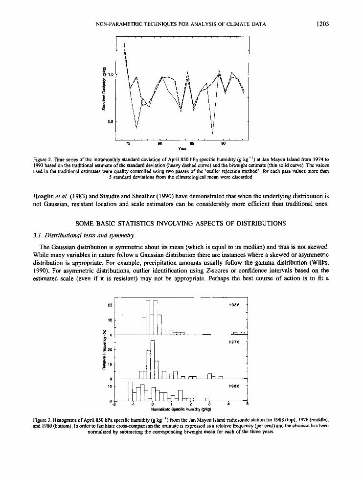
The final example of this subsection is intended to illustrate the benefits of resistant estimation (of scale) in a realistic setting. The data consist of 850 hPa specific humidity measured during April at the Jan Mayen Island radiosonde station (71"N, 8"W) and were obtained from an updated version of the archive maintained at the Geophysical Fluid Dynamics Laboratory (GFDL) by Oort (1983); these data were provided originally by Roy Jenne of the National Center for Atmospheric Research (NCAR). All available soundings during the period 1974- 1993 were used.

Two different estimates of the intramonthly standard deviation of April specific humidity are shown in Figure 2. The thin solid curve is the biweight standard deviation whereas the heavy dashed curve is the traditional standard deviation. For the traditional estimate quality control of the type typically performed was applied; for the biweight there was no explicit quality control. The quality control consisted of first using all available values to estimate a climatological mean and standard deviation and then discarding outliers (defined as values more than 5 standard deviations from the mean). Using this 'cleaned-up' sample the outlier rejection procedure was again applied.

As can be seen from Figure 2 the traditional and biweight estimates are quite similar most of the time. However, in a few instances the biweight gives much lower estimates. In particular the years 1976 and 1988 are characterized as the two lowest variability years by the biweight but as somewhat more variable than normal by the traditional estimate. These two cases will be examined in greater detail through the use of histograms. In addition, the year 1980 will be used as a reference year because the two methods yield almost identical values, characterizing it as one of the more highly variable years.

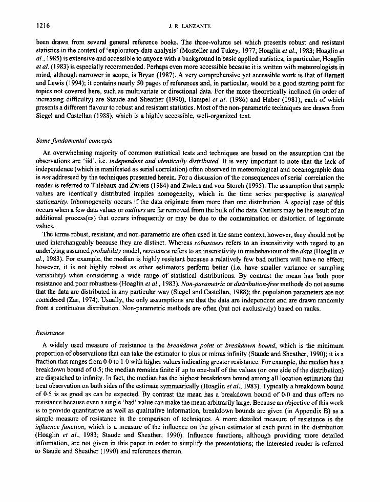
Histograms for the three selected years (1988, 1976 and 1980) are shown in Figure 3. Based on visual inspection it is apparent that for 1988 and 1976 there is peakedness and considerable concentration of mass near the centres of the distributions. In contrast, the distribution for 1980 has the bulk of its mass spread out over a greater range and over this range it is fairly flat. These histograms suggest that the biweight has produced estimates more in line with intuition. The misleading traditional estimates are at least partially the result of a few infrequent large values that occurred during 1988 and 1976. Cursory examination of daily time series (not shown) suggests that these are legitimate values representing relatively rare (but not unreasonable from a climatological standpoint) synoptic events characterized by intrusions of moist, lower latitude air. Another noteworthy point is the difference in the shape of the distributions between 198811976 and 1980 and their distinct non-Gaussian character. Simulations by

Table 11. Location, scale and maximum Z-score estimates based on a sample of 10 values consisting of the nine values: 1.01, 1.02, . . . , 1.09, plus 1000. Traditional is based on the conventional estimates of the mean and standard

deviation

Traditional Biweight

Mean 100.95 1.05 Standard deviation 315.90 0.03 Maximum Z-score 2.85 34340.29


75 80 85 90 YBar

Figure 2. Time series of the intramonthly standard deviation of April 850 hPa specific humidity (g kg-') at Jan Mayen Island from 1974 to 1993 based on the traditional estimate of the standard deviation (heavy dashed curve) and the biweight estimate (thin solid curve). The values used in the traditional estimates were quality controlled using two passes of the 'outlier rejection method'; for each pass values more than

5 standard deviations from the climatological mean were discarded

Hoaglin et al. (1 983) and Staudte and Sheather (1990) have demonstrated that when the underlying distribution is not Gaussian, resistant location and scale estimators can be considerably more efficient than traditional ones.

SOME BASIC STATISTICS INVOLVING ASPECTS OF DISTRIBUTIONS

3.1. Distributional tests and symmetry

The Gaussian distribution is symmetric about its mean (which is equal to its median) and thus is not skewed. While many variables in nature follow a Gaussian distribution there are instances where a skewed or asymmetric distribution is appropriate. For example, precipitation amounts usually follow the gamma distribution (Wilks, 1990). For asymmetric distributions, outlier identification using Z-scores or confidence intervals based on the estimated scale (even if it is resistant) may not be appropriate. Perhaps the best course of action is to fit a

20

10

0

10 - 1980 -

n -1 0 1 2 3 4 5

0 -2

NormeHzed Spedk Humldhy (&)

Figure 3. Histograms of April 850 hPa specific humidity (g kg-') from the Jan Mayen Island radiosonde station for 1988 (top), 1976 (middle), and 1980 (bottom). In order to facilitate cross-comparison the ordinate is expressed as a relative frequency (per cent) and the abscissa has been

normalized by subtracting the corresponding biweight mean for each of the three years

1204 J. R. LANZANTE

parametric distribution to the sample; another reasonable approach is use of some transformation that renders Gaussian values. Unfortunately in the course of exploratory data analysis, and particularly for large multivariate data sets, this may not be accomplished easily because of the lack of suitable fit, the large number of possible distributions or transformations, or a prohibitive amount of effort required. An alternative introduced here is to define separate measures of scale for the upper and lower tails of the unkown, asymmetric distribution.

The simple alternative suggested here is referred to as an asymmetric pseudo-standard deviation, which consists of an upper and a lower pseudo-standard deviation. The upper (lower) pseudo-standard deviation is defined as twice the distance between the upper (lower) quartile and the median divided by 1.349. These can be used to construct an asymmetric confidence interval for outlier flagging, etc., based on the same rationale as for a symmetric confidence interval based on the pseudo-standard deviation except that the upper and lower bounds are based on separate estimates of scale. An important caution is that asymmetry should not be assumed unless there is good a priori evidence (such as physical insight of the system) and/or a posteriori evidence (appropriate statistical testing). A consequence of the use of these asymmetric scale estimators (as shown in appendix B) is a considerable drop (about half) in efficiency compared with the symmetric counterpart (which has low efficiency itself). Because of the resulting low efficiency this approach may be practical only when the sample size is large and of course when the confidence that the distribution is truly asymmetric is high. It is also possible to define an asymmetric version of the biweight standard deviation for which the efficiency is far more reasonable (50 per cent); see Appendix B for details.

A measure of confidence in the asymmetry can be gained through a statistical test of the symmetry of a distribution. The method introduced here to test for asymmetry is a simple modification (see Appendix B for technical details) of a test for the equality of two sample distributions, which is of value in its own right. The modification is simply to partition a sample into two parts; each part is then treated as a separate sample in the two sample distributional test. One partition consists of all the values on one side of the median. The other partition consists of the values on the other side of the median reflected across the median. For a symmetric distribution one side of the distribution and the mirror image of the other side of the distribution will be indistinguishable.

Two non-parametric distributional tests that utilize ranks are presented here (see Appendix B for details) for use in testing asymmetry or for simply testing the equality of the medians of two distributions. The fist is the Wilcoxon-MamWhitney test, which can be used to test the equality of the medians of two distributions and is one of the most powerful non-parametric tests (Siegel and Castellan, 1988). An assumption of the Wilcoxon- Mann-Whitney test is that the two distributions have equal variances. Another two-sample test for the equality of medians in which equality of variances is not assumed (the Behrens-Fisher problem) is the robust rank-order test, which has essentially the same power efficiency as the Wilcoxo*MamWhitney test (Siegel and Castellan, 1988).

3.2. Distributional/symmetry example

The example used to illustrate the symmetry testing and confidence interval generation consists of all available values ofthe July 1000 hPa specific humidity at Barrow, Alaska from 1973 to 1989; these data were obtained from the GFDL radiosonde archive. The histogram of these values (shown in Figure 4) is intriguing because it indicates a positively skewed distribution with a sharp drop-off from the middle to the lower tail of the distribution. It can be speculated that the tendency for approximately a lower (hard) limit is due to the dominance of snow and ice melt during this time of year; the apparent lower limit is near the saturation specific humidity at the freezing point of water. The symmetry test is very confidently rejected with a significance level less than 0.001 per cent. The location and scale estimates for this sample are given in Table 111. The most striking aspect of the estimates is the fact that the upper pseudo-standard deviation is about twice that of its lower counterpart; the symmetric scale estimates are a compromise between the two. The asymmetric scale estimates seem reasonable from visual inspection because the upper half of the distribution is considerably more ‘strung out’ than the lower half.

Although the distribution in Figure 4 is asymmetric and unusual there is nothing about its appearance that suggests contamination with ‘bad’ outlying values. It seems reasonable to assume that it is a ‘clean’ sample from some unkown, asymmetric distribution. As such, a centred (1 - a) per cent confidence interval should exclude roughly u/2 per cent of the sample in each tail provided that a is not ‘too small’ for the given sample size.

NON-PARAMETRIC TECHNIQUES FOR ANALYSIS OF CLIMATE DATA

0 -2

250

ZOO

P

100 L H

50

-A 0 2

r

i

1205

Mean Median Standard deviation Pseudo-standard deviation Lower pseudo-standard deviation Upper pseudo-standard deviation

4.43 4.06 1.25 1.22 0.74 1.70

Confidence intervals for two levels (50 per cent and 95 per cent) based on the traditional, simple symmetric resistant and simple asymmetric resistant estimators are given in Table IV. The symmetric resistant interval fares poorly near the centre of the distribution (50 per cent level) as well as in the tails (95 per cent level). Because of a compromise estimate of scale it extends too far to the left (leaves too little in the left tail) but not far enough to the right (leaves too much in the right tail). The traditional interval fares well in the centre (50 per cent) due to compensating effects; it has the same problem with scale as the symmetric estimator, but has a (less reasonable) larger estimate of location which shifts the interval to the right. For the 95 per cent level the traditional estimate does poorly, with the same bias as the symmetric. The asymmetric interval fares well for both levels in terms of total coverage and balance between the tails. Of course when resistance is considered (not a factor in this example but more important in general) the traditional estimators are downgraded even more and the asymmetric resistant interval estimator emerges as an even clearer winner.

4. DISCONTINUITIES

4.1. The change-point problem

Statistical stationarity (homogeneity of a time series) is one of the most fundamental assumptions of most statistical tests and procedures. The change-point problem addresses a lack of stationarity in a sequence of random variables (values). Given a sequence of values a change-point is said to occur at some point in the sequence if all of the values up to and including it share a common statistical distribution, and all those after the point share another. The most common change-point problem involves a change (discontinuity) in the level (mean) and is the focus here. Testing for non-stationarity due to a change in the dispersion (variance) has been addressed recently by Downton and Katz (1993) although not in a resistant framework. Although it may be possible to develop such a resistant test based on the ANOVA approach of Best (1994) this will be left for future work because there are technical difficulties in extending the change-point test from the mean to the variance (Moses, 1963).

1206 J. R. LANZANTE

Table IV. Confidence intervals and percentage area outside those intervals for the data sample (Barrow 1000 hPa specific humidity) corresponding to Figure 4 and Table 111. The two confidence levels correspond to nominal coverages of 50 per cent and 95 per cent. Three different intervals are constructed: traditional (mean and standard deviation), simple symmetric resistant (median and pseudo-standard deviation) and simple asymmetric resistant (median and asymmetric pseudo-standard deviation). The actual coverage outside the interval is given for the lower tail, upper tail and total (sum of both tails)

Outside coverage @er cent)

Interval Lower Upper Total

50 per cent level Traditional Symmetric resistant Asymmetric resistant

95 per cent level Traditional Symmetric resistant Asymmetric resistant

[3.58, 5,271 [3.23, 4.881 [3.56, 5.211

[1.98, 6.881 [1.67, 6.451 [2.61, 7.391

25.0 25.9 10.1 25.8

2.5 0.9 0.7 2.0

25.0 23.5 30.0 24.0

2.5 5.3 7.7 2.7

50.0 49.4 40.1 49.8

5.0 6.2 8.4 4.7

There are a number of possible causes for discontinuities in climate-related time series. In recent years there has been increased concern with and awareness of inhomogeneities in data from surface (e.g. Easterling and Peterson, 1995) as well as upper-air stations (e.g. Elliott and Gaffen, 1991; Gaffen, 1994; Parker and Cox, 1995). Station moves (changes in elevation and or microclimate), change in instrumentation (new sensor or type of sensor) or recording practice (new time of observation, change in reduction algorithm) are just some of the things that can result in an artificial (non-climatic) inhomogeneity in station data. Artificial discontinuities exist in data sets produced operationally at numerical weather prediction centres (e.g. Barnston and Livezey, 1987; Lambert, 1990) due to periodic changes in the numerical model and/or analysis schemes. Discontinuities may occur in remotely sensed data as well; Chelliah and Arkin (1992) found that time series of outgoing longwave radiation contain multiple discontinuities owing to the use of different satellites (which have different crossing times and spectral windows). Of course not all discontinuities are artificial, such as the onset of Sahel drought (Demaree and Nicolis, 1990) or the shift in global climate variables around 197fj-1977 (Trenberth, 1990).

Easterling and Peterson (1 995) review various methods used by meteorologists to identify change-points and propose a new method. Approaches used in the past typically rely either on comparison with a reference series (which presumably does not have any of the discontinuities that may lurk in the series to be checked) constructed from neighbouring station(s) and/or the use of metadata (station history information). Examples of the former include Hanssen-Bauer and Forland (1994), Portman (1993) and Potter (1981), whereas Karl and Williams (1987) is an example of the latter. Although both approaches are worthwhile and valid, they each have disadvantages. Use of a reference series is dependent on the proper selection and weighting of the individual series. This approach may be feasible for surface stations, which normally have a number of suitable neighbours and for which most changes occur on a station-by-station basis. However, the upper-air network of stations is much sparser, so suitable neighbours may not exist; also, changes often occur by country, so neighbouring stations may have the same discontinuities. Station history information (metadata) is not always available or complete; in addition, some documented changes may not result in any discontinuity.

The method proposed here does not depend on ‘outside information’ such as reference series or metadata so it is more widely applicable. Also, it may be desirable to test for real climatic discontinuities where such information is not relevant. Nevertheless, when artificial change is the issue, once this method has identified candidate change- points it would be advisable to seek conka t ion using, for example, history information andor the results of this test applies to neighbouring stations. In particular, the fact that this test produces independent results for each station as opposed to the dependence inherent to methods involving reference series may be desirable. Finally, the procedure proposed here, unlike the other methods surveyed in the literature, utilizes non-parametric, resistant and robust principles, which makes it much more resilient in the presence of outliers and other non-standard behaviour.


Several principles may be utilized to interpret the results of independent application of the change-point test to different stations. A change-point found at a station but not at neighbouring stations suggests local causes, which are probably artificial. Change-points that are shared by some stations from the same country but which vanish across the border of nearby countries are also likely to be artificial. The concept of ‘neighbour’ can be extended to the vertical as well as to other climate variables. Real climate changes would probably have some coherence in the vertical and with other parameters. Finally, an abrupt climate change might be evidenced by a change of opposite sign at a distance of one-half a wavelength through a ‘teleconnection’. Although none of these approaches may be conclusive in isolation, when taken together they may present strong evidence of either natural or artificial change.

4.2. Overview of the change-point procedure

The procedure proposed here is an iterative one designed to search for multiple change-points in an arbitrary time series. It involves the application of a non-parametric test, related to the Wilcoxon-Ma-Whitney test discussed earlier, followed by an adjustment step; iteration continues until the test statistic is no longer significant or if other conditions occur (see Appendix B for details). Upon completion auxiliary measures are computed in order to aid the interpretation. Although the single change-point test is due to Siegel and Castellan (1 988), the procedure used to apply it to the multiple change-point problem and the auxiliary measures have been developed here.

The change-point test (Siegel and Castellan, 1988) uses a statistic computed at each point based on the sum of the ranks of the values from the beginning to the point in question. It seeks to find a single change-point in the series. Because it is based on ranks this test is not adversely affected by outliers and can be used when the time series has gaps; it is likely to be highly efficient (Siegel and Castellan, 1988). However, the significance of the test statistic cannot be evaluated confidently within 10 points of the ends of the time series, so change-points cannot be evaluated at the beginning or end; the technical details are given in Appendix B.

As the iteration proceeds each new change-point is added to an ordered list, which includes the first and last points of the series as well. At each step, consecutive points from the list are used to define change-point segments. A resistant location estimator (the median is used here) is computed separately for each segment and subtracted yielding an adjusted series that is resubmitted to the change-point test in the next iteration.

After completing iteration a change-point (or discontinuity) ‘signal to noise’ ratio which quantifies the magnitude of each discontinuity is computed. This quantity is computed for each change-point using the two adjacent change-point segments. This resistant signal-to-noise ratio expresses the magnitude of the discontinuity in terms of the ratio of the variance associated with the shift in level between the adjacent segments relative to the ‘background’ variability or ‘noise’ within each segment.

The procedure described above (and detailed in Appendix B) has been tested on a number of time series of different character, both real and contrived and has performed quite well. It is quite sensitive and is capable of detecting subtle changes. The amount of sensitivity can be controlled by the level of significance required. Obvious discontinuities tend to produce extremely significant results. Although experience suggests that a significance level of 1 per cent would be reasonable it is recommended that the investigator apply this procedure to a few ‘favourite’ time series to aid in deciding on the level of sensitivity (i.e. required significance).

Recently a new method for detecting discontinuities has been proposed by Easterling and Peterson (1 995). They have made comparisons of existing methods using simulations involving artificial time series for an ensemble of scenarios; the interested reader is directed to their paper for the details of the simulations. They have concluded that their method (hereafter referred to as the EP method) performs best of the methods examined. The method presented here (hereafter referred to as the L method) has been applied to an ensemble similar to theirs and the results (corresponding to their table 2) have been evaluated. In the interest of brevity only the major conclusions are presented. Based on the scenarios used the two methods appear to be comparable overall. The L method identified slightly fewer of the discontinuities but had a slightly lower ‘false alarm’ rate. Based on the different scenarios it appears as if the L method is a bit more sensitive (can detect weaker discontinuities) and performs better overall if the discontinuities are not too close (separated by at least 25 points). On the other hand the EP method seemed to have an advantage when the discontinuities were closely spaced (separated by only 10-15 points). The simulations were all based on Gaussian random numbers and did not include any outliers. Because the

1208 J. R. LANZANTE

EP method is based on least-squares linear regression, whereas the L method utilizes ranks, the L method has a distinct advantage in terms of resistance. The resistance of the L method can be appreciated in the Veracruz example, which is discussed below.

4.3. Change-point examples

The first example uses a time series of monthly anomalies of 200 hPa geopotential height at the Royal Observatory in Hong Kong from 1950 to 1960 and is shown in Figure 5. These data were taken from the TD54 data set which was obtained by Roy Jenne for use in the NMC/NCAR reanalysis project (Kalnay and Jenne, 199 1). Note that although 5 months were unavailable due to missing values in the original data set the change-point test is not adversely affected. The use of this particular time series was motivated by Gaffen (1994) who discovered a large discontinuity in 200 hPa temperature corresponding to the introduction (during July 1955) of a new radiation correction applied to the temperature measurements. The presence of the discontinuity in both time series is not surprising because geopotential height at radiosonde stations is derived directly from the measured temperature using the hydrostatic equation. Application of the change-point test identified July 1955 as the change-point; the significance is extreme (much better than 0.01 per cent). The discontinuity signal-to-noise ratio is 1.63, indicating that the variance associated with the change in means is more than one and a half times the variance associated with variability about the separate segment means.

Neglect of non-stationarity such as that associated with a discontinuity in the mean can have serious consequences in statistical estimation and testing. Such a sample is inhomogeneous because it represents a mixture distribution resulting from sampling two distinct populations. This is evident in Figure 6, which has histograms of the values of the time series in Figure 5 before (top) and after (bottom) correction for the discontinuity. Before correction the histogram is quite flat and hints at bimodality; after eliminating the discontinuity the resulting distribution is considerably narrower and looks much more reasonable (Gaussian). A quantitative assessment can be made by examining the biweight means and standard deviations computed from the whole series and separately from the two segments, as shown in Table V. In concert with visual inspection of the histograms, Table V confirms that neglect of the discontinuity (‘overall’) artificially inflates the standard deviation by a factor of nearly two.

In order to illustrate the effect of the discontinuity on the assessment of deviancy some additional statistics have been calculated and are given in Table V. These correspond to a hypothetical anomaly of -90 (m). The deviancy is quantified by expressing the anomaly as a Z-score. Ignoring the discontinuity (overall) this anomaly would be

-1 00 50 51 52 53 54 55 56 57 58 59 80 81

Y W

Figure 5. Time series of monthly 200 hPa geopotential height anomaly (m) at Hong Kong from 1950 to 1960. The monthly anomaly values (stars) are connected by a curve. The horizontal lines represent the biweight means of the two segments defined by the change-pint (circled

s w


L

10 - ’m I

n

- -80 -60 -40 -20 0 20 40 60 80

1

1 100

Height Anomaly (m)

Figure 6. Histogram of the values from Figure 5 before (top) and after (bottom) correction. Correction consists of normalization by subtraction of separate means for the two segments in Figure 5 defined by the change-point

Table V. Statistics computed for the entire time series (Hong Kong 200 hPa height) shown in Figure 5 (overall), separately for the left and right segments defined by the change-point and for the entire time series after the separate segment means have been subtracted (corrected). The Z-scores are computed for a hypothetical anomaly value of -90 (m) using the corresponding biweight mean and standard deviation. For ‘corrected’ the Z-scores differ depending on whether the hypothetical anomaly was placed originally in the left or right segment (l/r) as the segments have different means, which are used to correct the anomaly

Overall Left Right Corrected I/r

Biweight mean -0.17 30.09 -33.91 0.91 Biweight standard deviation 42.44 25.22 24.67 25.09 Z-score for -90 -2.12 -4.76 -2.27 -4.821-2.27

viewed as somewhat but not extremely deviant regardless of its position in the time series; the Z-score corresponds to a rate of occurrence of roughly 1 in 35. Intuitively (see Figure 5 ) it would seem that this anomaly should be regarded as much more deviant if it were to occur in the left segment as compared with the right segment. The Z- scores computed from the separate segment means and standard deviations confirm intuition, as do the calculations after correction; for the left segment the occurrence rate is roughly one in a million.

The next example, which illustrates the multiple change-point problem, uses monthly anomalies of 700 hPa geopotential height at Veracruz, Mexico from 1952 to 1992. These data were extracted from the four CD set ‘Radiosonde Data of North America, 19461992’ produced jointly by the National Climatic Data Center (NCDC) and the Forecast Systems Laboratory (FSL). The time series, change-points and segments shown in Figure 7 are based on application of the iterative change-point method requiring change-points to be significant at the 1 per cent level. This example is much more demanding than the previous one due to the multiple change-points and less dramatic change in means; the latter highlights the sensitivity of the method. The resistance of the method is indicated by the presence of several prominent outiers, particularly the one in the early 1960s. Several gaps due to missing data have no adverse effect. Statistics that quantify the change-point segments are given in Table VI. The probabilities indicate that the five change-points were all confidently identified. The change-points all have a lower signal-to-noise ratio than for the Hong Kong example (1.63), in particular, change-points three and five.

The final example of this section is concerned with a problem that may occur when averaging time series which have discontinuities. It is common practice in meteorology to compute regional, zonal, hemispheric, global, etc., averages based on a number of grid-point or station time series. If the constituent time series have discontinuities

1210

20

- - E 0 - 7a”

5 .20

I P

-40

J. R. LANZANTE

-

-

-

4 0 r 1

, I ; , 50 55 60 65 70 75 80 .85 90

-60

Year

Figure 7. Time series of monthly 700 hPa geopotential height anomaly (m) at Veracruz, Mexico from 1952 to 1992. The horizontal lines represent the biweight means of the segments defined by the change-points (circled stars)

Table VI. Statistics computed for multiple change-point analysis applied to the time series shown in Figure 7 (Veracruz 700 hPa height). Step refers to the iteration number, change-point (point) is the ordinal number of the change-point (from left to right in Figure 7), Z-statistic (Z) is the asymptotic 2-statistic associated with the change-point test (see Appendix B for details), followed by the probability associated with this 2 value, and the change-point or discontinuity signal to noise ratio ( R D N )

Step Point Z Probability RDN

1 2 11.95 <0.0001 1.25 2 1 8.37 <0~0001 0.69 3 4 4 4 8 <0~0001 1.09 4 3 3.81 0.0001 0.5 1 5 5 3.87 0~0001 0.29

that occur at different times but which delineate either systematic increases or decreases then the resulting average time series may mimic a trend even if none of the constituent series had one.

Historically, the introduction of new radiosonde humidity sensors has led systematically to artificial decreases in upper tropospheric humidity with time at some stations (Elliott and Gaffen, 1991). However, these decreases are usually evidenced as a step function in the station time series when the new sensor is introduced. The times of these changes generally vary by country, although even within a country introduction of new sensors may vary from station to station. This raises concern that averaging upper tropospheric humidity measurements may result in a ‘bogus’ downward trend.

The example used to illustrate this ‘bogus trend’ problem is based on alteration of the time series of Figure 5 , which has a prominent change-point in the middle of the time series. Two additional time series were constructed from this one by shifting the change-point either towards the beginning or end (by adding or subtracting means from one segment to values in the other segment). The three time series were then averaged together and are shown in Figure 8. This average time series exhibits an apparent downward trend from the first to the third change-points without any obvious discontinuities. A smoother trend could be obtained by averaging more time series.

NON-PARAMETRIC TECHNIQUES FOR ANALYSIS OF CLIMATE DATA 121 1

50 51 52 53 54 55 56 57 58 59 SO 61 Year

-100

Figure 8. Time series that is the average of the time series of Figure 5, with two altered versions of it. The two altered versions were produced by shifting the change-point (discontinuity) towards the beginning or end of the series (by adding or subtracting the segment mean from the

other segment to some of the values). The location of the change-points for the three series are indicated by the circled stars

5 . LINEAR ASSOCIATION

5.1. Correlation and regression

Correlation and simple linear regression are probably the most widely used techniques for assessing the linear relationship between two variables. Like the univariate measures discussed earlier these too may be affected adversely by data misbehaviour. Regression is also used in trend analysis which may be useful in assessment of either real climate change (such as ‘global warming’) or artificial change. Examples of artificial change include trends such as that associated with ‘drift’ in an instrument (e.g. ground-based thermometer or satellite sensor), the effect of urbanization on surface temperature, the change from ‘bucket’ to ‘intake’ sea-surface temperature measurements and the changeover from the use of the Beaufort scale to anemometers for wind speed.

The (Pearson product-moment) correlation coefficient is the most powerful parametric correlation (Siegel and Castellan, 1988); however, it may be affected adversely by outliers and for assessment of significance it requires that the observations are sampled from a bivariate normal distribution. A non-parametric alternative presented here is the Spearman rank-order correlation coefficient (Siegel and Castellan, 1988), which is computed by ranking (separately) the two variables and then correlating their ranks (see Appendix B for technical details).

One way to perform resistant regression is via three-group resistant regression (Hoaglin et al., 1983). For this method (see Appendix B for technical details) the sample is subdivided into three groups based on the abscissas. The median coordinates of the left and right groups are used to define a line which serves as a starting point for an iterative process; a special procedure ensures convergence to a final solution. The other resistant regression method presented here is based on the median of pairwise slopes (see Appendix B for technical details) and was used recently in the assessment of hydroclimatic trends (Lettenmaier et al., 1994). It involves the computation of the slopes defined by all possible pairs of points; the final slope estimate is the median of these values. Because significance tests are not provided for these regression techniques the significance of the Spearman correlation coefficient will be used instead.

The choice between these two techniques for resistant regression may well hinge on the sample size as well as the computing power available. For very small samples both are efficient (see Appendix B). As the sample size increases the pairwise slopes method becomes slightly more efficient, whereas the three-group method becomes much less efficient. This can be explained by the fact that the three-group method initially reduces the information from all of the points to a slope computed from just two summary points; the larger the number of points the larger the relative reduction (and ‘loss of information’). By contrast, the number of slopes computed by the pairwise slopes method increases with the sample size. Based on its greater efficiency and resistance the pairwise slopes

1212 J. R. LANZANTE

method seems preferable. Unfortunately the computational expense (number of pairs) grows explosively with the sample size so that for larger sample sizes it may be necessary to use the three-group method.

5.2. Correlation and regression examples

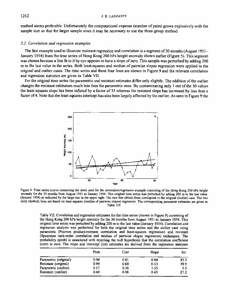
The first example used to illustrate resistant regression and correlation is a segment of 30 months (August 195 1- January 1954) from the time series of Hong Kong 200 hPa height anomaly shown earlier (Figure 5). This segment was chosen because a line fit to it by eye appears to have a slope of zero. This sample was perturbed by adding 200 m to the last value in the series. Both least-squares and median of pairwise slopes regression were applied to the original and outlier cases. The time series and these four lines are shown in Figure 9 and the relevant correlation and regression statistics are given in Table VII.

For the original time series the parametric and resistant estimates differ only slightly. The addition of the outlier changes the resistant estimators much less than the parametric ones. By contaminating only 1 out of the 30 values the least-squares slope has been inflated by a factor of 35 whereas the resistant slope has increased by less than a factor of 4. Note that the least-squares intercept has also been largely affected by the outlier. As seen in Figure 9 the

~

52 53 54 Year

Figure 9. Time series (curve connecting the dots) used for the correlatiodregression example consisting of the Hong Kong 200 Wa height anomaly for the 30 months from August 1951 to January 1954. This original time series was perturbed by adding 200 m to the last value (January 1954) as indicated by the large star in the upper right. The two thin (thick) lines correspond to the original (outlier) case. The two solid (dashed) lines are based on least-squares (median of painvise slopes) regression. The corresponding parameter estimates are given in

Table VII

Table VII. Correlation and regression estimates for the time series (shown in Figure 9) consisting of the Hong Kong 200 hPa height anomaly for the 30 months from August 195 1 to January 1954. This original time series was perturbed by adding 200 m to the last value (January 1954). Correlation and regression analysis was performed for both the original time series and the outlier case using parametric (Pearson product-moment correlation and least-squares regression) and resistant (Spearman rank-order correlation and median of pairwise slopes regression) techniques. The probability (prob) is associated with rejecting the null hypothesis that the correlation coefficient (corr) is zero. The slope and intercept (int) estimates are derived from the regression analyses

Rob COK Slope Int

Parametric (original) 0.94 0.01 0.04 43.3 Resistant (original) 0.99 0.00 0.13 39.5 Parametric (outlier) 0.17 0.26 I .33 5.5 Resistant (outlier) 0.69 0.08 0.45 27.2


2 1 5 0 0 hPa rlk\ , 1

0

Q -1

5 -2

1 2

s o

4:

-1

- 4 1 ' " " " " " " " " " ~ ' ~ ' ~ a 62 64 66 68 70 72 74 76 78 80 82 84 86 88 90

Year

Figure 10. Time series of tropically averaged monthly temperature (light curves) and specific humidity (dark curves) for 500 hPa (top) and 850 hPa (bottom) for 1963 to 1988. Each curve has been standardized to zero mean and unit variance. These curves represent a subset of the data

shown in Figure 3 of Sun and Oort (1995) and have been temporally filtered as described herein

resistant line attempts to represent the bulk of the data faithfidly whereas the least-squares line is skewed by a single outlier. The resistant fit is more reasonable and appealing.

The final example of this paper is taken from analyses performed by Sun and Oort (1 995) and Sun and Held (1 996), which relate tropically averaged temperature and humidity; the data, which represent temporally filtered spatial averages of an updated version of the grid-point values produced by Oort (1 983), were kindly provided by D.-Z. Sun. Figure 10 shows time series of tropically averaged monthly temperature (light curves), T, and specific humidity (dark curves), q, for the 500 (top) and 850 hPa levels (bottom) for the period 1963-1988. In order to facilitate cross-comparison each curve has been standardized to zero mean and unit variance. In general, variations in Tand q follow each other reasonably well at both levels. However, two major exceptions can be seen at 500 hPa. During 1968 there is a suspicious downward spike of Twhich is not reflected in q and is only very weakly apparent at 850 hPa. In addition, during the 1982-1983 El Niiio event, T and q uncharacteristically depart in opposite directions at 500 hPa. Sun and Oort (1995) suggest that departures such as these may be due partly to very unusual conditions during the 1982-1 983 event and partly to the irregular distribution of radiosonde stations. Because the reliability of radiosonde measurements decreases with the height above the surface, observational problems may be greater in the upper troposphere.

An x-y plot of the 500 hPa T and q from Figure 10 is shown in Figure 1 1. Each point is represented by a star except for the unusual periods near 1968 (circles) and 1982-1 983 (squares). It can be seen that points during the two unusual periods represent outliers. However, it is important to note that typical univariate quality control would not flag these points as outliers because neither their x nor y coordinates are outliers; they are outliers in the bivariate sense. This is another instance which demonstrates that good quality control does not obviate the need for resistant methods.

By chance it turns out that the two uncharacteristic time periods act in the same sense. As seen in Figure 11 the least-squares regression line (solid) is rotated clockwise from the resistant line (dashed) in an attempt to be more 'accommodating' to the outlying points. Sun and Held (1996) used these same data to examine the radiative feedback of water vapour as quantified by the fractional rate of increase of q with T (which is proportional to the slope of the line fit to T and q) . Figure 12 displays a plot of this quantity as a function of height (pressure level) in which the dark curve is based on least-squares regression and the light curve on resistant regression. The dashed curve is a reference curve based on the assumption of constant relative humidity. From this plot it can be seen that although least-squares and resistant regression differ only a little in the lower troposphere, at upper levels the resistant line is noticeably closer to the reference curve.

1214 J. R. LANZANTE

3

,. , 2 -

,

4 -2 0 2 4 Temperature (standardized)

-3

Figure 1 1. Plot of temperature ( 7 ) versus specific humidity (4) at 500 hPa using the data from the top of Figure 10. The abscissa and ordinate are standardized units. Each point is represented by a star except for points during the unusual periods December 1967 to April 1968 (open circles) and November 1982 to July 1983 (open squares). Two regression analyses have been performed using all of the values (stars, circles

and squares); the solid line is based on least-squares regression and the dashed line is the median of pairwise slopes estimate

Rate ol Fractional lnmase of q Wnh T (M)

Figure 12. Rate of fractional increase of specific humidity (4) with temperature ( r ) as a fhction of vertical pressure level (hPa) following Sun and Held (1996). The dark (light) curve is based on estimates derived from least-squares regression (median of pairwise slopes resistant regression) applied to the observed data from Figure 1 I . The dashed curve is a reference curve based on the assumption of constant relative

humidity and is solely a consequence of the Clausiudlapeyron relationship

6. SUMMARY AND DISCUSSION

Traditional statistical methods widely used in research are based on a number of fundamental assumptions which all too often are violated in practice. Violations of the assumptions considered here include the presence of outliers, non-Gaussian behaviour and statistical non-stationarity. Alternative techniques from resistant, robust and non- parametric statistics often can be used when these assumptions are not met. Although these alternative techniques are less likely to ‘break down’ in the presence of outliers or other data misbehaviour due to their increased resistance, they tend to be less efficient (i.e. have larger sampling variability) when the data are ‘well behaved’. An effort has been made here to present a couple of alternative techniques to be used in the estimation of location (central tendency), scale (spread or dispersion), and simple bivariate linear association (correlation and


regression); symmetry and the testing for differences in distributions has also been addressed. The simpler alternatives tend to be computationally and conceptually simpler at the expense of statistical efficiency. More sophisticated alternatives combine resistance with a high level of efficiency at the expense of some increased effort and complexity.

The problem of statistical inhomogeneity or non-stationarity (changes in the statistical distributional properties over time) is a violation of the most fimdamental assumption addressed here. A procedure has been developed to identify multiple step-function-like changes in the level (central tendency) over time by using a non-parametric ‘change-point’ test. Correction of time series to eliminate these discontinuities as well as trend removal (using a resistant technique) can go a long way towards satisfying the assumption of stationarity.

A couple of points that arose in some of the examples but which were not mentioned explicitly deserve comment for their more general applicability to all of the techniques presented here. In some of the examples, monthly anomalies were analysed for consecutive months. It was implicitly assumed that: (i) the values are independent and (ii) that the relationships are homogeneous across the seasonal cycle. To the extent that the values are serially correlated the significance levels are inflated. Possible ‘remedies’ include use of an ‘effective’ degrees of freedom (although strictly speaking this may not be valid), Monte Carlo simulation which incorporates the serial dependence, transformation of the data to yield independent values (such as via time series modelling techniques), or performing separate analyses for each month type (assuming independence at 1 year lag). Regarding the second point possible remedies include standardizing the values (dividing the anomalies by the standard deviation for the corresponding month) or performing separate analyses for each month; if the nature of the relationship is seasonally dependent then only the latter approach is valid because the set with mixed month types represents an inhomogeneous sample.

Although this paper has dealt only with basic statistical methods there is certainly no restriction on the application of resistant, robust and non-parametric techniques to more sophisticated methods such as multiple linear regression, ANOVA, empirical orthogonal function, canonical correlation, singular value decomposition, cluster, discriminant or spectral analysis, for example. One simple approach might be to apply resistant outlier removal as a pre-processing step. Another approach is to substitute resistant estimators in the advanced procedure. The second approach should be done only with caution because it may result in a change in the inherent properties of the technique; for example, do resistant variance components preserve the total variance? Instead it may be necessary to change the nature of the technique in order to obtain resistance; in this regard the reader is advised to examine the references highlighted in Appendix A.

In conclusion the methods and philosophy presented here are worthy of consideration in any statistical analysis. Certain types of problems benefit more and some practically require these techniques (such as data quality assessment and control). The challenge is issued here to investigators to consider the implicit assumptions of the statistical techniques that they employ.

ACKNOWLEDGEMENTS

1 wish to express appreciation to Tony Broccoli, Gabriel Lau, Becky Ross, David Cox and the anonymous reviewer for the constructive comments and corrections that they provided, and to Mike Alexander, Mike Timlin and Clara Deser for pointing out the tendency for the change-point test to identify changes associated with trends. Special thanks to GFDL librarian Gail Haller for her patience and persistence in obtaining many of the references needed to prepare this report. The TD54 data set and documentation were kindly provided by Roy Jenne and Will Spangler of NCAR. Thanks also to De-Zeng Sun, Bram Oort and Isaac Held for use of tropically averaged temperature and humidity data and the example relating to these quantities.

APPENDIX A: SOME CONCEPTS, THEORY AND CONSIDERATIONS

Suggested reading

Some theoretical aspects are presented in this appendix in order to further motivate the alternative techniques promoted in this paper and to make it easier to understand their properties. Much of the material for this paper has

1216 J. R. LANZANTE

been drawn from several general reference books. The three-volume set which presents robust and resistant statistics in the context of ‘exploratory data analysis’ (Mosteller and Tukey, 1977; Hoaglin et al., 1983; Hoaglin et al., 1985) is extensive and accessible to anyone with a background in basic applied statistics; in particular, Hoaglin et al. (1983) is especially recommended. Perhaps even more accessible because it is written with meteorologists in mind, although narrower in scope, is Bryan (1 987). A very comprehensive yet accessible work is that of Barnett and Lewis (1 994); it contains nearly 50 pages of references and, in particular, would be a good starting point for topics not covered here, such as multivariate or directional data. For the more theoretically inclined (in order of increasing difficulty) are Staude and Sheather (1 990), Hampel et al. (1986) and Huber (1 98 l), each of which presents a different flavour to robust and resistant statistics. Most of the non-parametric techniques are drawn fiom Siegel and Castellan (1 988), which is a highly accessible, well-organized text.

Some fundamental concepts

An overwhelming majority of common statistical tests and techniques are based on the assumption that the observations are ‘iid’, i.e. independent and identically distributed. It is very important to note that the lack of independence (which is manifested as serial correlation) often observed in meteorological and oceanographic data is not addressed by the techniques presented herein. For a discussion of the consequences of serial correlation the reader is referred to Thiebaux and Zwiers (1984) and Zwiers and von Storch (1 995). The assumption that sample values are identically distributed implies homogeneity, which in the time series perspective is statistical stationarity. Inhomogeneity occurs if the data originate from more than one distribution. A special case of this occurs when a few data values or outliers are far removed from the bulk of the data. Outliers may be the result of an additional process(es) that occurs infrequently or may be due to the contamination or distortion of legitimate values.

The terms robust, resistant, and non-parametric are often used in the same context, however, they should not be used interchangeably because they are distinct. Whereas robustness refers to an insensitivity with regard to an underlying assumed probability model, resistance refers to an insensitivity to misbehaviour of the data (Hoaglin et al., 1983). For example, the median is highly resistant because a relatively few bad outliers will have no effect; however, it is not highly robust as other estimators perform better (i.e. have smaller variance or sampling variability) when considering a wide range of statistical distributions. By contrast the mean has both poor resistance and poor robustness (Hoaglin et al., 1983). Non-parametric or distributionfree methods do not assume that the data are distributed in any particular way (Siegel and Castellan, 1988); the population parameters are not considered (Zar, 1974). Usually, the only assumptions are that the data are independent and are drawn randomly from a continuous distribution. Non-parametric methods are often (but not exclusively) based on ranks.

Resistance

A widely used measure of resistance is the breakdown point or breakdown bound, which is the minimum proportion of observations that can take the estimator to plus or minus infinity (Staude and Sheather, 1990); it is a fraction that ranges from 0.0 to 1 .O with higher values indicating greater resistance. For example, the median has a breakdown bound of 0.5; the median remains finite if up to one-half of the values (on one side of the distribution) are dispatched to infinity. In fact, the median has the highest breakdown bound among all location estimators that treat observation on both sides of the estimate symmetrically (Hoaglin et al., 1983). Typically a breakdown bound of 0.5 is as good as can be expected. By contrast the mean has a breakdown bound of 0.0 and thus offers no resistance because even a single ‘bad’ value can make the mean arbitrarily large. Because an objective of this work is to provide quantitative as well as qualitative information, breakdown bounds are given (in Appendix B) as a simple measure of resistance in the comparison of techniques. A more detailed measure of resistance is the in$uence function, which is a measure of the influence on the given estimator at each point in the distribution (Hoaglin ef al., 1983; Staude and Sheather, 1990). Influence hnctions, although providing more detailed information, are not given in this paper in order to simplify the presentations; the interested reader is referred to Staude and Sheather (1 990) and references therein.


Effciency

Another measure used widely to characterize statistical performance is ejiciency, which is a ratio of variances (i.e. the sampling variabilities) of two different estimators of a quantity, or equivalently a ratio of sample sizes (Siegel and Castellan, 1988). Efficiency is a measure of performance relative to some standard. If for example (for a given sample size) an estimator has an efficiency of 0.8 relative to some standard estimator, then the variance of the standard estimator is 80 per cent of that of the variance of the estimator in question. Equivalently, the standard estimator requires a sample size only 80 per cent of that of the estimator in question in order to have the same variance as the estimator in question. Although the efficiency may be any non-negative number, typically the standard used is an estimator that is ‘optimal’; in this case the efficiency will not exceed 1.0. For a Gaussian distribution the efficiency of the median to the mean is about 64 per cent and does not vary greatly with sample size (Hoaglin et al., 1983). In this paper, as is commonly the case, efficiency is evaluated for a Gaussian distribution; generally speaking this is a pessimistic measure because the efficiencies of the alternative techniques presented here are usually larger (than 1) when the data are not Gaussian.

Other useful variations on efficiency exist. Asymptotic relative efficiency is the limiting value of efficiency taken when the sample size tends to infinity (Staudte and Sheather, 1990); asymptotic efficiency, unlike efficiency in general is not a function of sample size. Although the above measures of efficiency are used in reference to estimates of parameters there is also a measure of efficiency used in conjunction with statistical tests. The power ejiciency of a test is the ratio of sample sizes such that both tests have the same power (Siegel and Castellan, 1988). The power of a test is the probability of correctly rejecting the null hypothesis in contrast to the significance which is the probability of incorrectly rejecting the null hypothesis.

An attempt is made to provide (in Appendix B) some measure of efficiency for the procedures presented in this paper. Many of these were taken from the references cited and some were derived through simulation. As a result of the varied sources the efficiencies are of different types. This is not a problem because generally the efficiencies vary much more between the different statistical estimators or procedures than among the different types of efficiencies.

Remarks

Constancy of the underlying statistical distribution across a collection of observations has been cited as one of the most fundamental assumptions shared by most common statistical methodology. Resistant, robust and non- parametric techniques provide alternative procedures that relax this assumption. This paper presents some of these alternative techniques, illustrating their utility via example, and quantitative measures (breakdown bound and efficiency) derived from statistical theory. The breakdown bound is a measure of resistance to misbehaviour of the data, whereas efficiency measures the performance relative to some standard (usually a common parametric estimator/test assuming a Gaussian distribution). Typically, resistance and efficiency are competing demands; resistant procedures are less efficient when the underlying distribution is Gaussian but provide much better results when the sample contains outliers or is otherwise non-Gaussian. However, through the use of more sophisticated methods it is possible to gain considerable resistance while sacrificing only a little efficiency. Loosely speaking the breakdown bound can be used to address the question ‘what do I gain by using an alternative technique when the data are misbehaved?’ whereas the efficiency addresses the question ‘what do I lose when the data are well- behaved?’.

At this point a comment of some practical considerations seems in order. The alternative techniques presented in this paper have two associated computational drawbacks. First, they require the data to be ranked or sorted. Because it is common to archive data in map form (all locations for a given time together) rather than in time series form (all times for a given location together) it may be necessary as a preliminary step to reorganize a data set to the latter form. Second, these techniques require more arithmetic computation. However, given the significant advancement in computing speed and data archival capacity in recent years these concerns should not hinder the use of the techniques described in this paper.

1218 J. R. LANZANTE

APPENDIX B: PROPERTIES (BREAKDOWN BOUNDS AND EFFICIENCIES), FORMULAE AND TECHNICAL DETAILS

This appendix presents the formulae and provides other details needed to implement the methods presented in this paper along with relevant references. It also cites breakdown bounds and efficiencies fiom the literature (where available); the reader may find these useful in comparing the resistant methods with one another and with the traditional methods.

In a few instances efficiencies were not available in the literature andor were of the different types (of efficiencies) so Monte Car10 simulations using Gaussian random numbers were performed in order to provide this information. The results of these simulations are given in Tables BI and BII and are cited below when appropriate. It should be noted that the use of the Gaussian reference in the efficiency simulations presented here is a conservative approach towards evaluating resistant alternatives; as shown by simulations (Hoaglin et al., 1983; Staudte and Sheather, 1990), when the underlying distribution is not Gaussian, resistant estimators are typically more efficient (sometimes considerably) than the traditional ones. This remark is also applicable to the cited efficiencies that are Gaussian as well.

Median

The median is a simple estimator of location with high resistance (breakdown bound is 0.5; Staudte and Sheather, 1990) and an efficiency of about 0.64 (Hoaglin et al., 1983); see also Table BI for efficiencies. The median (M) is the ‘middle’ value of a distribution and is estimated (fiom a sample of n values) by:

Pseudo-standard deviation (based on the interquartile range)

A simple estimate of scale is the pseudo-standard deviation. One way to define a pseudo-standard deviation (sps) is based on the interquartile range (IQR). This scale estimator has a breakdown bound of 0.25 (Staudte and

Table BI. Efficiencies of selected estimators estimated from the variances over 10 000 trials of Gaussian random numbers for two different sample sizes (5 and 30); the third column has efficiencies (see elsewhere in Appendix B for the types) cited from the literature; the cited values of 0.64,0.37 and 0.87 are taken fiom Hoaglin ef al. (1983), Staudte and Sheather (1990), and Hoaglin et al. (1983). The efficiency is defined as the ratio of the variance of the reference estimator (mean for location and standard deviation for scale) to that of the selected estimator. By definition the reference estimators have efficiencies of 1.0. Note the consistency of simulated and cited values as well as the relative lack of sensitivity to sample size (also c o n h e d by simulations not shown for intermediate sizes). The efficiencies seem to be approaching the cited asymptotic values for a

sample size of 30

n = 5 n = 30 Cited

Mean Median Biweight mean Standard deviation Pseudo-standard deviation Asymmetric pseudo-standard deviation Biweight standard deviation Asymmetric biweight standard deviation

1 .oo 0.70 0.83 1 .oo 0.66 0.28 0.78 0.48

1 .oo 0.67 0.93 1 .oo 0.39 0.17 0.84 0.45

1 .oo 0.64

1 .oo 0.37

-

- 0.87


Sheather, 1990) but an efficiency of only 0.37 (Staudte and Sheather, 1990); see also Table BI. The interquartile range is defined as:

IQR = q0.75 - 40.25 (B2)

where q0.75 (qo.25) is the upper (lower) quartile. If the sample size ( n ) is even then the upper (lower) quartile is the median of the largest (smallest) n/2 observations. If the sample size is odd then the upper (lower) quartile is the median of the largest (smallest) (n+1)/2 observations. The pseudo-standard deviation (sps) based on the interquartile range is:

sPs = IQR/1*349. (B3)

For a Gaussian population the standard deviation is identically equal to the pseudo-standard deviation defined in this manner.

An asymmetric pseudo-standard deviation can be defined for the lower (upper) half of the distribution by replacing the IQR in equation B3 with twice the distance between the median and the lower (upper) quartile; its efficiency is 0.17 for a sample size of 30 (see Table BI).

Biweight mean and standard deviation

The biweight (Hoaglin et al., 1983) is a more sophisticated estimator belonging to the category known as redescending estimators. Its influence function returns to zero at some distance away from the centre of the distribution; this distance is determined by a parameter (c). The biweight mean ( j b i ) is highly resistant (a breakdown bound of 0.5; Hoaglin et al., 1983) and fairly efficient (roughly 0.9 as determined by simulations herein; see Table BI). The biweight standard deviation (sbi) is also highly resistant (a breakdown bound of 0-5; Hoaglin et al., 1983) and fairly efficient (0.87 for a sample size of 20; Hoaglin et al., 1983); see also Table BI for efficiencies of the biweight standard deviation and its asymmetric version.

The biweight estimate is a weighted average such that weighting decreases away from the centre of the distribution. All values beyond a certain critical distance from the centre (controlled by the parameter ‘c’) are given zero weight. A ‘c’ value between 6 and 9 is recommended (Hoaglin el al., 1983); for the Gaussian case, c = 6 (9) censors values more than 4 (6) standard deviations from the mean. In this paper c = 7.5 (censors values more than 5 standard deviations away) has been used. The censoring is performed using preliminary (resistant) estimates of location (median) and scale (median absolute deviation), which are used to determine the weights.

First the median (M) and median absolute deviation (MAD) are estimated. The MAD is the median of the absolute values of the deviations of the sample values from the median. A weight (ui) corresponding to each of the n observations (Xi) is computed as follows:

ui = (xi - M ) / ( c x MAD). 034)

For any lui l2 1 .O, set ui = 0.0 to accomplish the censoring. The biweight estimate of the mean is:

Similarly, the biweight estimate of the standard deviation is:

It should be noted that because the biweight weighting h c t i o n places more emphasis on values near the centre (of mass) of the distribution, for distributions that are skewed (or otherwise asymmetric) the biweight mean will be closer to the median than to the arithmetic mean.

An asymmetric biweight standard deviation can be defined for the lower (upper) half of the distribution by computing the biweight standard deviation of a sample consisting of all of the values less (greater) than the biweight mean plus these same values reflected across the biweight mean; its efficiency is 0.45 for a sample size of

1220 I. R. LANZANTE

30 (see Table BI). The reflection is analogous to that by equation (B16) except that the reflection is with respect to the biweight mean instead of the median.

WilcoxowManw Whitney distributional test for location)

The Wilcoxon-MamWhitney test is used to test for equality of medians based on two samples with parent populations that are assumed to have equal variances. It is one of the most powerful non-parametric tests; compared with the t-test its power efficiency is about 0.95 even for moderate sample sizes and not much less for small sizes (Siegel and Castellan, 1988). It is resistant because it is based on ranks.

In this test the two samples are combined and then ranks are assigned to the combined sample. The test statistic is based on the sum of the combined sample ranks corresponding to one of the original samples. If the original samples are distributed differently then the sums of the ranks for the two samples will be significantly different.

Suppose two samples consisting of values Xi and 5 have sample sizes of n, and n,,, respectively, where n = n, + n,,. Rank the values in the set formed by combining the Xand Y values. Let SR, be the sum of the ranks of the Xvalues from this combined sample. Define the following quantities:

SC"* = nx(n + 1)/2 037)

(B8) sSR = [nxny(n + I)/ 12]0'5

6 = +0.5 SR, <&fit

-0.5 SR,>S~t 0.0 SR, = &fit

z = (SR, - &fit + ~ ) / s s R . 0310) Note that 6 is a continuity correction. The test statistic z is asymptotically -N(O, 1) (i.e. normal with a mean of 0 and a standard deviation of 1). A two-tailed test using a normal probability table can be used if either n, > 10 or ny > 10, otherwise use table J of Appendix I in Siegel and Castellan (1988).

Robust rank-order distributional test for location)

The robust rank-order test is similar in nature to the WilcoxowManwWhitney test in that it is also a test for equality of medians based on two samples; by contrast the rank-order test does not assume that the parent populations have equal variance (i.e. it deals with the well-known Behrens-Fisher problem). It has essentially the same power as the Wilcoxon-MamWhitney test (Siegel and Castellan, 1988). It is resistant because it is based on ranks.

The robust rank-order test starts by computing the ranks of the combined sample. Next, for each value in each sample it is necessary to count the number of observations from the other sample having a lower rank. Means and variances of these counts can be combined to form a test statistic.

Suppose two samples consisting of values of Xi and 5 have sample sizes of n, and n,,, respectively, where n = n, + ny. Rank the values in the set formed by combining the X and Y values. For each Xi define NXi to be the number of Y values having a lower rank than Xi from this combined sample. Similarly, define NYj to be the number of X values having a lower rank than 5. Compute the following quantities:

= 2 N&/n, i= 1

"Y

j = I = C N5/ny


The test statistic z is asymptotically -N(O,l). A two-tailed test using a normal probability table can be used if either n, > 12 or n,, > 12, otherwise use table K of Appendix I in Siegel and Castellan (1988).

Symmetry test for skewness)

A test of symmetry has been devised here by transforming a sample into two samples, which are then tested using a location (median) test such as the WilcoxowManwWhitney or robust rank-order test. As noted above both of these tests have high efficiency and, because they are based on ranks, are resistant. The transformation is based on rejlecting half of the sample (for example, the half which is less than the median) across the median. If the original sample is symmetric about the median then the upper half and the reflected lower half will have the same location (median). To perform the transformation, first estimate the median (M) of the original sample. Next partition the original set of values into XL values (XG values) for values less (greater) than M. Transform the XL values into Y values by reflecting them across the median:

Y = M + (M - XL). (B 16)

The distributional test is then applied to the XG values and Y values.

Change-point test (based on location)

There are three aspects to the change-point procedure: the test for a single change-point (given by Siegel and Castellan, 1988), the iterative scheme (developed here) to test for multiple change-points and a diagnostic quantity, a signal-to-noise ratio (also developed here). Although the efficiency of the (single) change-point test has not been analysed explicitly, because it is based on a WilcoxowMamWhitney type rank sum statistic it is likely to be highly efficient (Siegel and Castellan, 1988). It is resistant because it is based on ranks.

Test for a single change-point. The change-point test presented here is used to determine if, and locate a point in the time series at which, the median changes. The test is based on summing the ranks of the data from the beginning to each point in the series; each raw sum is adjusted by the amount expected on average, which is linearly proportional to the point in the time series. The maximum of the adjusted statistic is assessed for significance.

The test procedure in testing for a single change-point in a series of xl. values of length n begins by finding the rank (Ri ) corresponding to each Xi. At each point ( i ) in the series compute the sum of the ranks from the beginning to that point (SR,) and from each of these an adjusted sum (SA,) at each point:

I

SR; = C Rj j = I

SA, = I(2SR;) - i(n + 1)l. (B 18)

Next find the maximum of the SA; values (over points 1 to n - 1). Suppose the maximum value of the SA; values occurs at point nl and suppose W is the corresponding value of the sum of the ranks at nl (i.e. SR,,); define the following:

n2 = n - n l (B 19)

1222 J. R. LANZANTE

6 = +0*5 W < Wcit -0.5 W > Wc,, 0.0 w = went

z = (W - Went + d)/sw. 0323)

The test statistic z is asymptotically - N(0,l). A two-tailed test using a normal probability table can be used if both nl > 10 and n2 > 10, otherwise use table J of appendix I in Siege1 and Castellan (1988).

Multiple change-point procedure. The iterative procedure to search for multiple change-points is based on application of the (single) change-point test followed by adjustment (see below) of the series. In the subsequent iteration the change-point test is applied to the adjusted series. Iteration continues as long as the significance of each new change-point is less than an a priori specified level (for example 0.01). As an alternative or supplement in significance assessment the robust rank-order test, which does not assume equality of variance, could be used. This supplemental test has been used for the examples shown here as well as other cases; although the significance levels did differ somewhat (only by a significant amount when both tests indicated extremely significant results) it was rare that the number of change-points selected would differ. Besides significance there are several other stopping or selection criteria that have been used. Iteration should stop if the change-point is one of the first or last 10 points of the series because the estimates are not reliable at the ends of the series. In the rare case of a repeated change-point seek a secondary maximum (of the SA statistic) that does not coincide with or lie adjacent to an existing change-point; stop if no such secondary mamimum exists or if it is not significant.

For each iteration there is an ordered list of Nchange-points (zi values). Each change-point is an ordinal number corresponding to a value in the original time series (which consists of n points). The list is cumulative so that each new point is inserted into the existing list. By defining additional beginning (zo = 0) and ending (zN+, = n) points in this list (which than has N + 2 points) a set of N + 1 change-point segments can be defined. The kth segment goes from point 1 + zk-1 to z k .

The adjustment applied at each iteration involves normalization by subtracting from each point the median of its segment. If desired (purely for cosmetic reasons) the median of the original time series may be added back to each value. It should be noted that it is important to retain the prior change-points in defining segments in the adjustment (i.e. to use an accumulated list). Adjustment by defining only two segments based on the most recent change-point can lead to non-convergence in that often previously defined change-points are reselected and the segment adjustments oscillate. The reason is that by discarding previous change-points the two current segments become a mixture of populations, the median of which may not be representative owing to the inhomogeneity. Also, proceeding by applying the single change-point test separately to each new segment (i.e. subdivide the series as each new change-point is added) will not work well in general because as the segment size decreases end effects become more dominant.

Because of a pathological condition it is possible that the change-point test may falsely identify as a change- point the centre of a time series which has a trend. The reason is that the means of the left and right sides of a trend line are different; in some sense this mimics the effect of a discontinuity. If the change-point test is applied iteratively to a series with a trend the procedure will typically subdivide the trend segment in half several times, thus identifying several false change-points. Although this problem may not occur for weak trends, the tendency for this to occur increases as the strength (magnitude of the correlation) of the trend increases. Detrending the time series before subjecting it to the change-point procedure, although recommended when there is an obvious trend, is not a fool-proof solution because the problem will still occur if just a portion of the series has a trend.

A straightforward and very effective solution to this problem has been determined. After each new change-point is identified it is necessary to compute two ‘noise-statistics’ (defined below under ‘Change-point signal-to-noise ratio’): one assuming the new change-point indicates a discontinuity and the other assuming it is the centre of a trend segment. If the former is smaller in magnitude than the latter then iteration continues as described previously. If the latter is smaller then a trend adjustment is made, this (most recent) change-point (a ‘trend-point’) is deleted


from the change-point list and then iteration continues with the next application of the change-point test. The trend adjustment consists of detrending (using resistant regression) the segment defined by the two change-points (from the z list) adjacent to the trend-point.

Change-point signal-to-noise ratio. In order to have a quantitative measure of the discontinuity implied by each change-point, a ratio, which can be thought of as a sort of resistant change-point or discontinuity signal-to-noise ratio, has been developed. This is a useful quantity that supplements the significance values provided at each step of the iteration. Keep in mind that after the first change-point, the significance values are somewhat artificial in that they apply to the adjusted rather than the original time series. As defined here, this measure is the ratio of the variance associated with the discontinuity of the resistant mean (i.e. the ‘signal’) to the resistant variance that remains after the discontinuity has been removed (i.e. the ‘noise’). In other contexts the discontinuity variance might be considered noise as well. In order to have both high resistance and efficiency, biweight estimators have been used.

Associated with a given change-point are two adjacent segments. First compute the biweight estimates of the means of these two segments (z and for the left and right segments). Suppose the left and right segments consist of nL and n R values, where n = nL + nR. Define an overall mean (2) and then an estimate of the variance associated with the change-point discontinuity (s;):

x = [ ( n L E ) + ( n R ~ ) ] / n

_ _ To compute the noise variance first normalize the left and right segments by subtracting XL (XR) from all of the

values in the left (right) segment. The noise variance ( s i ) is the (biweight) variance over the two normalized segments combined. Finally, the change-point or discontinuity signal-to-noise ratio (RDN) is:

Note that the noise variance (sk) is the same as the ‘discontinuity noise variance’ mentioned above in association with testing for a false chang-point due to a trend (trend-point). For this purpose a ‘trend noise variance’ can be defined in a similar fashion as the noise (biweight variance) over the combined segment (combining the left and right segments) after it has been detrended (normalized) using resistant regression. Thus, these two noise quantities measure the noise about a step-function change and the noise about a linear trend.

The RDN is a useful measure that can be used to eliminate change-points which are so weak that they are ‘of no practical importance’. The minimum required value of RDN is of course subjective and must be chosen by the user for each particular application; experience with this method suggests a value of at least 0.05 or 0.10, although in some cases a value as high as 0.3-0.5 may be appropriate. Experience has also shown that the utility of RDN as a measure of the strength of a change-point may be degraded somewhat as the length of the two adjacent sements becomes larger. To lessen this effect one could compute RDN from segments which are not allowed to exceed a certain limit (for example 50 points away from the change-point).

Spearman rank-order correlation

The Spearman rank-order correlation coefficient is a non-parametric measure of linear association based on correlation of ranks. Its efficiency compared with the Pearson product-moment correlation is about 0.91 (Siege1 and Castellan, 1988). It is resistant because it is based on ranks.

The fist step is to rank (separately) the two samples which consist of n values each. Let RDi be the difference of the ranks for the ith pair of values. Compute the sum of the rank differences (SRD), Spearman correlation coefficient (r,) and test statistic (t) as follows:

1224 J. R. LANZANTE

n

i= 1 SRD=CRD;

t = r,[(n - 2)/(1 - (B29)

A two-tailed test may be performed using the fact that the test statistic is asymptotically - tn-2; it is recommended that n be at least 20. For the smaller sample sizes use table Q of appendix I in Siege1 and Castellan (1988).

Three-group resistant regression

Three-group resistant regression (Hoaglin et al., 1983) is based on dividing the sample into three groups and fitting a line to the centre points of the left and right groups. An iterative process refines the estimate of the line. A special adjustment (B34) is needed to ensure convergence; without this adjustment the slope estimates oscillate between opposite signed values in certain pathological cases. This method has a breakdown bound of 1/6 (0.17) because the median (which has a breakdown bound of 1/2) is used in each of the three groups (Hoaglin et al., 1983). The efficiency is not given in the literature but simulations performed here (see Table BII) suggest that the asymptotic efficiency (relative to least-squares regression) is roughly 0.5 and that the efficiency increases as the sample size decreases (to about 0-9 for a sample size of 5). The iterative procedure ( i is the iteration number) is given below in the form of a set of (eight) steps.

Partition the sample into three equal (or nearly equal) sized groups on the basis of the ranks of the x-coordinates (abscissas). For the left and right groups compute the medians of the x-coordinates and the medians of the y-coordinates. Define left and right summary points from the x and y medians: (xL, yL) and (xR, yR). Compute the initial ( i = 0) estimate of the slope (b) from the left and right summary points:

b0 = h 7 - fi)/(xR - xL). 0330)

Compute the residual (resk) for each point (k) in the left and right groups using the estimate of the slope (bi) for the current iteration ( i ) :

resk = yk - (b;xk). 0331)

Determine the median value of the residuals (res, values) in the left (rl;) and right (rri) groups and compute their difference (AJ:

Ai = rr; - rl;. (B32)

If i = 0 then estimate the slope as follows and go to step (iv):

bl = b0 + [AO/(xR - XL)]. 0333)

If i > 0 then go to step (vii). If IAil < E (where E is some small number; 0.001 has been used here) then use the estimate from the current iteration (b;) as the final slope estimate (b) and go to step (viii). Otherwise, if the algebraic signs of bi and bi- I are different estimate the slopes as follows and go to step (iv):

(B34) bi+, = b; - [Ai(bi - bi-I)/(A; - A,-,)].

h+l = bi + [&/(xR - XL)I-

Otherwise, estimate the slope as follows and go to step (iv):

0335)


(viii) Compute the residuals for all of the points (i.e. from all three groups) using equation (B31) and the final slope estimate (b). The estimate of the intercept (a) is the median of all of these residuals. The three-group resistant regression line is:

>k = a + (bxk).

Table BII. Efficiencies of slope estimates from two resistant regression methods (three-group resistant regression and the median of pairwise slopes regression) estimated from the variances over 10 000 trials of Gaussian random numbers for several sample sizes (5, 10,20, 50, 100 and 1000). The simulation using pairwise slopes for a sample size of 1000 was not performed due to the computational expense. The efficiency is defined as the ratio of the variance of the reference estimator (least-

squares regression) to that of the selected estimator

Sample size

5 10 20 50 100 1000

Three-group 0.90 0.72 0.62 0.57 0.59 0.54 Median of pairwise slopes 0.88 0.88 0.9 1 0.97 0.95 -

Median of pairwise slopes regression

Median of pairwise slopes regression (Hoaglin et al., 1983) is based on computing the slope between every possible pair of points and taking the median of these values. The breakdown bound of this method is about 0.29 (Hoaglin et al., 1983). The efficiency is not given in the literature but simulations performed here (see Table BII) suggest that the asymptotic efficiency (relative to least-squares regression) is roughly 0.95 but that the efficiency may decrease to roughly 0.85-0.90 for very small sample sizes ( < 10).

It is necessary to compute the slope ( b k ) between each possible pair of points, (xi, y i ) and (xj yj):

If n is the number of points then there will be n(n - 1)/2 pairwise slopes; in fact there may be less if xi =xi for any i andj. The final slope estimate (b) is the median of the bk values. Using this slope estimate compute the residuals for all n points:

resi = yi - (hi).

j i = a + (hi).

(B38)

0339)

The intercept estimate (a) is the median of these residuals and the regression equation is:

REFERENCES

Barnett, V. and Lewis, T. 1994. Outliers in Statistical Dafa, Wiley, New York, 584 pp. Barnston, A. and Livezey, R. 1987. ‘Classification, seasonality and persistence of low-frequency atmospheric circulation patterns’, Mon. Wea.

Best, D. 1994. ‘Nonparametric comparison of two histograms’, Biometrics, 50, 53S541. Bryan, J. 1987. Course Notes on Robust and Resistant Statistical Methods, American Meteorological Society, Boston, MA, 104 pp. Chelliah, M. and Arkin, P. 1992. ‘Large-scale interannual variability of monthly outgoing long-wave radiation anomalies over the global

Collins, W. and Gandin, L. 1990. ‘Comprehensive hydrostatic quality control at the National Meteorological Center’, Mon. Wea. Rev., 118,

Demaree, G . and Nicolis, C. 1990. ‘Onset of Sahelian drought viewed as a fluctuation-induced transition’, Q. J. R. Meteorol. Soc., 116,

Downton, M. and Katz, R. 1993. ‘A test for inhomogeneous variance in time-averaged temperature data’ J. Climate, 6, 244a2464 Easterling, D. and Peterson, T. 1995. ‘A new method for detecting undocumented discontinuities in climatological time series’ Int. J.

Elliott, W . and Gaffen, D. 1991. ‘On the utility ofradiosonde humidity archives for climate studies’, Bull. Am. Meteorol. SOC., 72, 1507-1520.

Rev., 115, 108S1126.

tropics’, J. Climate, 5, 371-389.

2752-2767.

22 1-238.

Climatol., 15, 36S377.

1226 J. R. LANZANTE

Gaffen, D. 1994. ‘Temporal inhomogeneities in radiosonde temperatue records’ J. Geophys. Res., 99(D2), 3667-3676. Hampel, F., Ronchetti, E., Rousseeuw, P. and Stahel, W. 1986. Robust Statistics: the Approach bused on Influence Functions, Wiley, New

Hanssen-Bauer, I. and Forland, E. 1994. ‘Homogenizing long Norwegian precipitation series’, J. Climate, 7, 1001-1013. Hoaglin, D., Mosteller, F. and Tukey, J. 1983. Understanding Robust and Exploratory Data Analysis, Wiley, New York, 447 pp. Hoaglin, D., Mosteller, F. and Tukey, J. 1985. Exploring Data Tables, Trendr and Shapes, Wiley, New York, 527 pp. Huber, P. 1981. Robust Statistics, Wiley, New York, 308 pp. Kalnay, E. and Jenne, R. 1991. ‘Summary of the NMCMCAR reanalysis workshop of April 1991’. Bull. Am. Meteorol. SOC., 72, 1897-1904. Karl, T. and Williams, C. 1987. ‘An approach to adjusting climatological time series for discontinuous inhomogeneities’, J. Clim. Appl.

Lambert, S. 1990. ‘Discontinuities in the long-term northern hemisphere 500-millibar heights dataset’, J. Climate, 3, 147%1484. Lettenmaier, D., Woods, E. and Wallis, J. 1994. ‘Hydro-climatic trends in the continental United States 1948-88’, J. Climate, 7, 586-607. Moses, L. 1963. ‘Rank tests of dispersion’, Ann. Math. Statist., 34, 973-983. Mosteller, F. and Tukey, J. 1977. Data Analysis and Regression. A Second Course in Statistics, Addison-Wesley, Reading, MA, 588 pp. Oort, A. 1983. Global Atmospheric Circulation Statistics, 1958-1973, Professional Paper 14, National Atmospheric and Oceanic

Parker, D. and Cox, D. 1995. ‘Towards a consistent global climatological rawinsonde data-base’, Int. J. Climatol., 15, 473496. Portman, D. 1993. ‘Identifying and correcting urban bias in regional time series: surface temperature in China’s northern plains’, J. Climate, 6,

Potter, K. 1981. ‘Illustration of a new test for detecting a shift in mean precipitation series’, Mon. Wea. Rev., 109, 204C~2045. ShifRer, R. 1988. ‘Maximum Z scores and outliers’, Am. Statist., 42, 7-0. Siege], S. and Castellan, N. 1988. Nonparametric Statistics For The Behavioural Sciences, McCraw-Hill, New York, 399 pp. Staudte, R. and Sheather, S. 1990. Robust Estimation and Testing, Wiley, New York, 357 pp. Sun, D-Z. and Held, 1. 1996. ‘A comparison of modeled and observed relationships between interannual variations of water vapor and

Sun, D-Z. and Oort, A. 1995. ‘Humidity-temperature relationships in the tropical troposphere’, J. Climate, 8, 1974-1987. Thiebaw, H. and Zwiers, F. 1984. ‘The interpretation and estimation of effective sample size’, J. Clim. Appl. Meteorol., 23, 80&811. Trenberth, K. 1990. ‘Recent observed interdecadal climate changes in the Northern Hemisphere’, Bull. Am. Meteorol. SOC., 71, 98W93. Wilks, D. 1990. ‘Maximum likelihood estimation for the gamma distribution using data containing zeros’, J. Climate, 3, 1495-1501. Zar, J. 1974. Biostatistical Analysis F’rentice-Hall, Englewood Cliffs, NJ, 620 pp. Zwiers, F. and von Storch, H. 1995. ‘Taking serial correlation into account in tests of the mean’, J. Climate, 8, 336351.

York, 502 pp.

Meteorol., 26, 1744-1 763.

Administration, Rockville, MD. [Available from GFDLMOAA, P.O. Box 308, Princeton, NJ 08542.1

2298-2308.

temperature’, J. Climate, 9, 665-675.

Documents

RESISTANT, ROBUST AND NON-PARAMETRIC … journal of climatology, vol. 16, 1197-1226 (1996) resistant, robust and non-parametric techniques for the analysis of climate data: theory