ECONOMIC GROWTH CENTERYALE UNIVERSITY

P.O. Box 208269New Haven, CT 06520-8269

http://www.econ.yale.edu/~egcenter/

CENTER DISCUSSION PAPER NO. 885

RESIDENTIAL SEGREGATION IN GENERAL EQUILIBRIUM

Patrick BayerYale University

Robert McMillanUniversity of Toronto

and

Kim RuebenPublic Policy Institute of California

May 2004

Notes: Center Discussion Papers are preliminary materials circulated to stimulate discussions and critical comments.

We would like to thank Fernando Ferreira for outstanding research assistance. Thanks also to Pedro Cerdanand Jackie Chou for help on assembling the data. We are grateful to Pat Bajari, Steve Berry, Dennis Epple,Tom Nechyba, Holger Sieg and Chris Timmins for many valuable discussions, and to Joe Altonji, GregoryBesharov, Maureen Cropper, David Cutler, James Heckman, Vernon Henderson, Phil Leslie, Costas Meghir,Robert Moffitt, Michael Riordan, Steve Ross, Kerry Smith, Jon Sonstelie, Chris Taber, Chris Udry, and JacobVigdor for additional valuable comments. We also thank conference participants at the AEA, ERC, IRP,NBER, PET, SITE, and SIEPR, and seminar participants at Brown, Chicago, Chicago-GSB, Colorado,Columbia, Duke, Johns Hopkins, Northwestern, NYU, PPIC, Stanford, Toronto, UC Berkeley, UC Irvine,UCLA, and Yale for useful suggestions. This research was conducted at the California Census Research DataCenter; our thanks to the CCRDC, and to Ritch Milby in particular. We gratefully acknowledge financialsupport for this project provided by the National Science Foundation under grant SES-0137289 and by thePublic Policy Institute of California.

This paper can be downloaded without charge from the Social Science Research Network electroniclibrary at: http://ssrn.com/abstract=546485

An index to papers in the Economic Growth Center Discussion Paper Series is located at: http://www.econ.yale.edu/~egcenter/research.htm

Residential Segregation in General Equilibrium

Patrick Bayer, Robert McMillan, and Kim Rueben

Abstract

This paper studies the causes and consequences of racial segregation using a new general

equilibrium model that treats neighborhood compositions as endogenous. The model is estimated

using unusually detailed restricted Census microdata covering the entire San Francisco Bay Area,

and in combination with a rich array of econometric estimates, serves as a powerful tool for carrying

out counterfactual simulations that shed light on the causes and consequences of segregation. In

terms of causes, and contrasting with prior research, our GE simulations indicate that equalizing

income and education across race would be unlikely to result in significant reductions in racial

segregation, as minority households would sort into newly formed minority neighborhoods. Indeed,

among Asian and Hispanic households, segregation increases. In terms of consequences, this paper

provides the first evidence that sorting on the basis of race gives rise to significant reductions in the

consumption of local public goods by minority households and upper-income minority households

in particular. These consumption effects are likely to have important intergenerational implications.

Keywords: Segregation, General Equilibrium, Endogenous Sorting, Urban Housing Market,Locational Equilibrium, Counterfactual Simulation, Discrete Choice

JEL Codes: H0, J7, R0, R2

1

1 INTRODUCTION

Residential segregation on the basis of race and ethnicity is a phenomenon present in

every metropolitan area throughout the United States.1 Given its pervasive nature, the causes and

consequences of segregation have attracted considerable academic scrutiny. Researchers

investigating the underlying causes have attempted to assess the extent to which racial

segregation can be explained by differences in income, wealth, and education across race;2,3 in

terms of consequences, a number of papers have explored the effects of living in a segregated

neighborhood on individual outcomes.4

This paper studies the causes and consequences of segregation from a new perspective.

The primary economic analysis builds on a series of theoretical papers that have analyzed

residential sorting in a general equilibrium setting. Important examples include work by Epple,

Filimon and Romer (1984, 1993), Benabou (1993, 1996), Fernandez and Rogerson (1996, 1998),

and Nechyba (1999, 2000). All feature models with multiple communities, heterogeneous agents

who are mobile across communities, and community compositions that are endogenous to the

sorting process. As these papers demonstrate, general equilibrium sorting models provide a

coherent framework for analyzing interdependent individual decisions that drive aggregate

outcomes,5 proving particularly useful in tracing the complex and otherwise difficult-to-predict

effects of policy. Thus Fernandez and Rogerson (1996) provide a tractable analytical framework

for examining the effects of school finance reforms that both change school funding and alter

household location decisions. In a more complex setting, Nechyba (2000) sets out a

computational model that explores the effects of school vouchers using general equilibrium

simulations, allowing for households to choose schools and relocate across neighborhoods. In

1 In the year 2000, for example, black households in the Detroit metropolitan area lived in Census tracts that were on average almost 80 percent black and only 15 percent white, while in marked contrast, white households lived in Census tracts that were only 5 percent black and 90 percent white. In the San Francisco Bay Area, where racial divisions might seem less severe, the typical black household lives in a neighborhood with more than nine times the fraction of black households found in neighborhoods resided in by the typical white household. 2 See Massey and Denton (1987, 1989, 1993), Miller and Quigley (1990), Harsman and Quigley (1995), Borjas (1998) and Bayer, McMillan, and Rueben (2004a), among others. 3 A related body of work has explored whether racial segregation is driven by the decentralized preferences of households as they make their residential location decisions or by some form of centralized discrimination. Cutler, Glaeser, and Vigdor (1999) examine segregation patterns over the full course of the 20th century, concluding that centralized racism was much mo re important in driving segregation in the earlier part of the century. Other notable papers include King and Mieszkowski (1973), Yinger (1978), Schafer (1979), and Kiel and Zabel (1996). 4 See Borjas (1995) and Cutler and Glaser (1997) for important contributions. 5 Epple, Filimon and Romer (1984, 1993) focus on conditions needed to prove existence in multi-community models that incorporate voting.

2

both papers, allowing for mobility gives rise to effects in general equilibrium that would not be

apparent in partial equilibrium, where household sorting is abstracted from.

In common with the applied theory literature, the current paper also specifies a general

equilibrium multi-community model that treats neighborhood compositions as endogenous.

However, it explores the potential of equilibrium sorting models in a new direction, analyzing

locational equilibria in actual metropolitan areas. This gives rise to two differences relative to

prior literature. In terms of the sorting model itself, we provide a very rich parameterization of

household preferences, allowing the household location decision to be driven by a wide range of

potentially relevant choice characteristics, including endogenous characteristics such as the race

of one’s neighbors – the rich data we have access to make this feasible. The model permits

household preferences to vary in a very flexible way with observable household characteristics,

so that households of different races can place a different valuation on having neighbors of a

given race – a horizontal model is natural in this context.6

Second, while prior work has typically used an analytic approach or relied on calibration

of a few main parameters, we estimate a wide range of demand parameters directly using

unusually detailed restricted Census microdata. These cover the entire San Francisco Bay Area,

providing a wealth of household characteristics and detailed information on household locations

and characteristics of neighbors. Our estimation approach draws on the notion of revealed

preference: examining actual location decisions vary on average with household characteristics,

one can learn how preferences for housing and neighborhood attributes vary with these

characteristics. An important feature of our approach is that it accounts for an important

endogeneity problem arising due to the correlation of neighborhood sociodemogaphics with

unobserved housing and neighborhood quality. Among the rich array of preference estimates that

we recover, it is clear that racial interactions in the utility function are powerful.

6 As noted in Epple, Filimon and Romer (1993), there is an important tradeoff to be made between incorporating voting in multiple-community models on the one hand and abstracting from the political process entirely on the other. The inclusion of voting necessitates restrictions to be placed on preferences in order to ensure existence of an equilibrium. Important recent papers by Epple and Sieg (1999) and Epple, Romer and Sieg (2001) estimate equilibrium models that include voting over the level of public goods, restricting households to have shared rankings over a single public goods index. In this paper, we abstract from the political process to focus on racial segregation, a phenomenon that is primarily the product of decentralized location decisions made by heterogeneous households. Doing so allows us to specify preferences in a very flexible way. We also note that in a Californian context, state financing of education has left relatively little discretion over public goods determination at the local level.

3

In combination with these econometric estimates, our equilibrium sorting model provides

a powerful tool for shedding new light on the causes and consequences of residential segregation

in a general equilibrium setting. We address two hypotheses, prompted by a striking empirical

observation: neighborhoods with both a high fraction of minority households and even moderate

levels of income (and education) tend to be in relatively short supply in many metropolitan areas -

this is readily apparent from Table 12 below. The short supply of such neighborhoods implies

that a household’s choice of neighborhood along other dimensions, including school quality,

neighborhood income and education, is often tied together very explicitly with race. This has the

effect of raising the implicit price that minority households pay for these neighborhood amenities,

as consuming more of these neighborhood amenities typically requires living in a neighborhood

with fewer minorities, while the opposite is typically true for white households.7

Our first hypothesis, prompted by the short supply problem, relates to the causes of

segregation. The previous literature universally suggests that an elimination of racial differences

in income, wealth, or education would decrease segregation: we hypothesize that segregation

could in fact increase once general equilibrium considerations are taken into account. In

particular, as minority households move up the income distribution, the distribution of available

neighborhoods will necessarily change. Because predominantly minority neighborhoods with

even moderate income and education levels are in short supply in most metropolitan areas and

would presumably be desirable to minority households, the increased formation of such

neighborhoods could lead to increasing segregation among minorities, working against any

segregation reduction due to the more even distribution of sociodemographic characteristics

across race.

A natural way to address this hypothesis is to compare the current equilibrium and a new

equilibrium in which racial differences in important socio-demographics have been eliminated.

We accomplish this using counterfactual simulations that shift many minority households up the

income distribution and then calculate a new sorting equilibrium for the entire metropolitan area,

allowing house prices to adjust and new types of neighborhood to form endogenously –

descriptive or partial equilibrium approaches have no adequate way of accounting for this kind of

possibility. Our results indicate that the elimination of racial differences in income (or education)

would lead to a moderate increase in the segregation of the high-income members of each major

7 The impact of the bundling of housing and neighborhood attributes in models of location choice is analyzed in Bayer (1999). The importance of issue bundling in a political economy context has been studied in Besley and Coate (2001).

4

racial group in the Bay Area and to an increase in the overall segregation of Asian and Hispanic

households. Partial equilibrium predictions of the model work in the opposite direction.8

Our second hypothesis relates to the consequences of segregation. In contrast with the

previous literature, which has emphasized the effects of living in a segregated neighborhood on

various individual outcomes, we draw attention to the way that race alters residential location

decisions in the first place. Accordingly, we advance the hypothesis that racial sorting in the

housing market serves to lower the consumption of a wide variety of neighborhood amenities by

minority households, pointing specifically to the implicit price mechanism described above. In

particular, when the size of a minority population is relatively small and its members relatively

poor on average, racial sorting in the housing market tends to raise the implicit price that

households in this group face for neighborhood amenities, thereby leading to a reduction in their

consumption.

We address this hypothesis by comparing the current equilibrium and a new equilibrium

in which racial factors have been eliminated from the household choice process: a comparison of

consumption patterns for households of different races and income levels in the current versus

new equilibrium will then reveal whether consumption of neighborhood attributes is significantly

affected. Our general equilibrium simulations provide the first evidence in the literature that

sorting on the basis of race itself (whether driven by preferences directly or discrimination) leads

to large reductions in the consumption of public safety and school quality by all black and

Hispanic households and large reductions in the housing consumption of high-income black and

Hispanic households.9 These effects are likely to have a significant impact on the inter-

generational persistence of racial differences in education, income, and wealth.

The rest of the paper is organized as follows: Section 2 outlines the key feature of our

San Francisco Bay Area dataset. Using these data, Section 3 provides evidence on the

distribution of neighborhoods available in the housing market as well as the actual neighborhood

8 One concern with this counterfactual simulation is that it assumes the general structure of racial preferences would be unaffected by the elimination of racial differences in income or education. In practice, major changes in the distribution of income or education across race might affect racial preferences – for example, with more high-income blacks in a metropolitan area for example, segregating forces could be weakened. To address this concern, we provide additional evidence based on an analysis of segregation patterns across the 330 US metropolitan areas, the results indicating that the elimination of racial differences tends to increase segregation when there are many minority households. See Section 8 below. 9 We remain agnostic throughout this paper as to whether these interactions arise as the result of the preferences of each race for living with neighbors of the same race or discrimination in the housing market. While this distinction has important welfare implications, the point made here concerning the impact of racial interactions on the consumption of housing and neighborhood attributes remains regardless of which explanation prevails. We discuss this issue in greater detail below.

5

choices that households in different race and income categories make. This descriptive evidence

motivates our two hypotheses. Sections 4, 5 and 6 describe the main analytical tool used in this

paper - an equilibrium model of residential sorting, describing the model, its estimation, and the

estimated preference parameters in turn. Section 7 uses the estimated model to conduct a series

of general equilibrium simulations that provide direct evidence on our central hypotheses.

Section 8 provides additional evidence using 2000 Census data from across metropolitan areas,

and Section 9 concludes.

2 DATA

The main analysis conducted in this paper is facilitated by access to restricted Census

microdata for 1990. These restricted Census data provide the detailed individual, household, and

housing variables found in the public-use version of the Census, but also include information on

the location of individual residences and workplaces at a very disaggregate level. In particular,

while the public-use data specify the PUMA (a Census region with approximately 100,000

individuals) in which a household lives, the restricted data specify the Census block (a Census

region with approximately 100 individuals), thereby identifying the local neighborhood that each

individual inhabits and the characteristics of each neighborhood far more accurately than has

been previously possible with such a large-scale data set.

For our primary analysis, we use data from six contiguous counties in the San Francisco

Bay Area: Alameda, Contra Costa, Marin, San Mateo, San Francisco, and Santa Clara. We focus

on this area for two main reasons: because it is reasonably self-contained, and because the area is

sizeable along a number of dimensions, including over 1,100 Census tracts, and almost 39,500

Census blocks, the smallest unit of aggregation in the data. The sample consists of just over

242,000 households.

The Census provides a wealth of data on the individuals in the sample – race, age,

educational attainment, income from various sources, household size and structure, occupation,

and employment location.10 In addition, it provides a variety of housing characteristics: whether

the unit is owned or rented, the corresponding rent or owner-reported value,11 number of rooms,

10 Throughout our analysis , we treat the household as the decision-making agent and characterize each household’s race as the race of the ‘householder’ – typically the household’s primary earner. We assign households to one of four mutually exclusive categories of race/ethnicity: Hispanic, non-Hispanic Asian, non-Hispanic Black, and non-Hispanic White. 11 As described in the Data Appendix, we construct a single price vector for all houses, whether rented or owned. Because the implied relationship between house values and current rents depends on expectations about the growth rate of future rents in the market, we estimate a series of hedonic price regressions for each of over 40 sub-regions of the Bay Area housing market. These regressions return an estimate of the

6

number of bedrooms, type of structure, and the age of the building. We use these housing

characteristics directly and in constructing neighborhood characteristics, characterizing stock of

housing in the neighborhood surrounding each house, as well as neighborhood racial, education

and income distributions based on the households within the same Census block group, a Census

region containing approximately 500 housing units. We merge additional data describing local

conditions with each house record, constructing variables related to crime rates, land use, local

schools, topography, and urban density. For each of these measures, a detailed description of the

process by which the original data were assigned to each house is provided in a Data Appendix.

The list of the principal housing and neighborhood variables used in the analysis, along with

means and standard deviations, is given in the first two columns of Table 1.

3 NEIGHBORHOOD SEGREGATION AND CONSUMPTION PATTERNS

These detailed data for the San Francisco Bay Area help bring to light two striking

aspects of neighborhood choice in the housing market equilibrium: there is a shortage of

neighborhoods with both a high fraction of minorities and even moderate levels of neighborhood

amenities; and minority households face a higher implicit price for such amenities than white

households do.

Segregation Patterns. Before turning to these, we first describe the general pattern of

segregation in the Bay Area by examining average racial exposure rates. These exposure rates

characterize the average racial composition of the neighborhoods in which households in a

particular sociodemographic category (e.g., high-income Asian households) reside;12 throughout

the portion of our analysis based on the Bay Area, we use Census block groups to define

neighborhoods.

The top panel of Table 2 reports average racial exposure rates by race. The measures

shown in the first column imply, for instance, that Asians in the Bay Area live in Census block

groups that are on average 23 percent Asian, 7 percent black, 12 percent Hispanic, and 57 percent

white. Comparing the racial exposure rates to the population of the Bay Area as a whole, a clear

pattern emerges, with households of each race residing with households from the same race in

proportions significantly higher than their proportions for the full Bay Area. The middle panel

ratio of house values to rents for each of these sub-regions and we use the average of these ratios for the Bay Area, 264.1, to convert monthly rent to house value for the purposes of reporting results at the mean. 12 A variety of segregation measures are available, and while no single measure is perfect, we choose to work with the exposure rate measures because they are easy to interpret and can be decomposed in a variety of meaningful ways.

7

shows the pattern of exposure for the top and bottom income quartile of households of each race,

along with the fraction of households in each race-income category. For example, the average

exposure of blacks to other blacks declines from 49 percent for those in the lowest quartile of the

income distribution to only 24 percent – still more than triple the fraction of blacks in the Bay

Area as a whole.

The bottom panel of Table 2 makes clear that high-income minority households, and

high-income blacks in particular, have a significant propensity to live with poorer households of

the same race. It reports the average exposure of households in the top quartile of the overall

income distribution for each race to households of the same race in each income quartile. The

second row, for example, shows that blacks in the top quartile of the income distribution live on

average in neighborhoods that consist of 9.8 percent blacks in the bottom quartile of the income

distribution and 3.5 percent blacks in the top quartile. Thus blacks in the top income quartile are

‘over-exposed’ to blacks in the poorest quartile, living on average in neighborhoods with almost

three times the fraction of these households in the Bay Area as a whole.13

Neighborhood Choices. To motivate our two central hypotheses more directly, Tables 3 and 4

describe the distribution of neighborhoods in which households of each race in the top and

bottom quartile of the income distribution reside, respectively. In each case, neighborhoods are

ranked by the fraction of households of the same race, and deciles of the distribution are then

reported. Focusing first on the second panel of Table 3, which shows the distribution of

neighborhoods in which high-income black households reside, the first column provides average

household, housing, and neighborhood characteristics for the 10 percent of high-income black

households that live in neighborhoods with the lowest fraction of black households,

neighborhoods in which less than 2 percent of the population is black. As one reads across the

columns, the neighborhoods have a larger fraction of black households by construction; the final

column indicates that fully 10 percent of blacks in the top income quartile reside in

neighborhoods in which over 76 percent of the population is black.

What emerges from Table 3 is the striking range of neighborhoods in which high-income

blacks reside. Comparing the neighborhoods at either end of the spectrum, the levels of school

quality, public safety, average neighborhood income, and fraction college-educated are each more

than 2 standard deviations greater in the high-income neighborhoods versus the high-minority,

13 While not as extreme as for blacks, the average exposure of high-income Asians to other Asians also remains well above the fraction of Asians in the Bay Area as a whole. As Panel C makes clear, however, in the case of high-income Asians, much of this overall exposure to other Asians results from a particularly strong exposure to other high-income Asians rather than to low-income Asians.

8

low-income neighborhoods. The pattern for high-income Hispanics is remarkably similar to that

for black households, as those neighborhoods with the highest fraction of Hispanics also possess

substantially lower average incomes, less educated neighbors, worse schools and higher crime

rates. For Asians, the pattern is qualitatively similar although much less marked, while for high-

income white households, increases in the consumption of local public goods and other

neighborhood socioeconomic measures are generally accompanied by an increase in the fraction

of white neighbors.

The patterns shown in Table 3 are suggestive of two important aspects of neighborhood

choice in the current Bay Area housing market equilibrium. First, the consumption of school

quality, public safety, neighborhood income and education is strongly negatively correlated with

the fraction of neighbors of the same race for black and Hispanic households. This suggests that

these households are partially constrained in the current Bay Area equilibrium, being confronted

by a shortage of minority neighborhoods with even moderate levels of desirable neighborhood

attributes.14 It is likely that an improvement in the availability of predominantly black and

Hispanic neighborhoods with even moderate levels of average income would be very attractive to

these households. This relates directly to our first hypothesis, as we would expect such

neighborhoods to form more easily with an increase in the fractions of black and Hispanic

households in the upper quartiles of the income distribution.

Second, while the increased consumption of neighborhood amenities comes at the

expense of increased housing prices for high-income households of each race, these increases are

accompanied by sharp decreases in the fraction of households of the same race for black and

Hispanic households but increases in the fraction of households of the same race for whites.

Given segregating racial preferences (as we find below), this implies that black and Hispanic

households face a price of consuming these neighborhood amenities that is implicitly higher than

the price faced by white households. Thus if race were removed as a consideration in the location

decision, along the lines of our second hypothesis, the implicit price that minority households

would face in choosing neighborhoods with more neighborhood amenities would fall, leading

them to choose neighborhoods more in line with those chosen by high-income black households

living in predominantly white neighborhoods.15

14 In the Bay Area in 2000, while predominantly Asian and white neighborhoods span the spectrum of average income levels, only six of the 659 tracts with income levels above that of the median tract, less than one percent, were more than 20 percent black. 15 The direct observation that, for instance, fully 30 percent of black households in the top income quartile, with income around $92,000, live in neighborhoods in which the average household income is less than $40,000 indicates that this is likely to be the case.

9

In a similar fashion, Table 4 reveals that black and Hispanic households in the bottom

income quartile also face an implicit price of neighborhood amenities that exceeds the direct

costs. While not as marked as for households in the top income quartile, the increased

consumption of these neighborhood amenities is again accompanied by sharp decreases in the

fraction of households of the same race for black and Hispanic households. Thus we anticipate

that racial sorting in the housing market also raises the implicit price of neighborhood amenities

for low-income black and Hispanic households, although perhaps not a starkly as for high-income

households.

An alternative potential explanation for the differences across the neighborhoods shown

in Tables 3 and 4 is that, within each of these race-income quartile groups, households have

heterogeneous demands for neighborhood characteristics and socioeconomics. This is certainly

part of the story.16 However, a proper test requires one to control directly household sorting on

the basis of other factors such as income, wealth, education, household structure, and

employment locations. To this end, we now describe a model of residential sorting that explicitly

incorporates these factors.

4 A MODEL OF RESIDENTIAL SORTING

This section sets out the principal analytical tool that we use to explore segregation as a

general equilibrium phenomenon - an equilibrium model of a self-contained urban housing

market in which households sort themselves among the set of available housing types and

locations. The model consists of two key elements: the household residential location decision

problem and a market-clearing condition. While it has a simple structure, the model allows

households to have heterogeneous preferences defined over housing and neighborhood attributes

in a very flexible way; it also allows for housing prices and neighborhood sociodemographic

compositions to be determined in equilibrium.

We estimate this model using rich individual data, appealing to the notion of revealed

preference - specifically that the residential location decision reveals preferences for a wide range

of housing and neighborhood attributes. By examining how location decisions vary, on average,

with household characteristics such as income, education, and race, one can learn how

preferences for the housing and neighborhood attributes vary with these sociodemographic

characteristics. Once the broad set of preference parameters in the model have been estimated,

16 For instance, the average income of the high-income black households that reside in the neighborhoods with the fewest black households is in fact larger ($112,000 on average) than for those that reside in the neighborhoods with the highest fraction of blacks ($91,000).

10

we then use the estimates and the equilibrium model to conduct a series of general equilibrium

simulations designed to shed new light on the causes and consequences of segregation.

The Residential Location Decision. We model the residential location decision of each

household as a discrete choice of a single residence from a set of houses available in the market.

The utility function specification is based on the random utility model developed in McFadden

(1973, 1978) and the specification of Berry, Levinsohn, and Pakes (1995), which includes choice-

specific unobservable characteristics.17 Let Xh represent the observable characteristics of housing

choice h including characteristics of the house itself (e.g., size, age, and type), its tenure status

(rented vs. owned), and the characteristics of its neighborhood (e.g., school, crime, and

topography). We use the notation Z to represent the average sociodemographic characteristics

of the corresponding neighborhood, writing it separately from the other housing and

neighborhood attributes to make explicit the fact that these characteristics are determined in

equilibrium.18 Let ph denote the price of housing choice h and, finally, let dhi denote the distance

from residence h to the primary work location of household i. Each household chooses its

residence h to maximize its indirect utility function Vhi:

(1) ihhh

iph

iZh

iX

ih

hpZXVMax εξααα ++−+=

)(.

The error structure of the indirect utility is divided into a correlated component associated with

each house that is valued the same by all households, ξh, and an individual-specific term, εih. A

useful interpretation of ξh is that it captures the unobserved quality of each house, including any

unobserved quality associated with its neighborhood.19

Each household’s valuation of choice characteristics is allowed to vary with its own

characteristics, Zi, including education, income, race, employment status, and household

composition. Specifically, each parameter associated with housing and neighborhood

characteristics and price, αij, for j ∈ {X, Z , d, p}, varies with a household’s own characteristics

according to:

17 Discrete choice applications in the urban economics literature include Anas (1982), Quigley (1985), Gabriel and Rosenthal (1989), Nechyba and Strauss (1998), Bajari and Kahn (2001). Only the latter paper includes choice-specific unobservables. Brock and Durlauf (2001) discrete choice models with social interactions. 18 This component of the utility function allows for endogenous sorting on the basis of race, as in Schelling (1969, 1971), as well as other characteristics such as income and education. 19 We employ an indirect utility function that is linear in housing prices. Alternative specifications of the indirect utility function could certainly be estimated, as the linear form is not essential to the model.

11

(2) ∑=

+=R

r

irrjj

ij Z

10 ααα ,

with equation (2) describing household i’s preference for choice characteristic j.

Characterizing the Housing Market. As with all models in this literature, the existence of a

sorting equilibrium is much easier to establish if the individual residential location decision

problem is smoothed in some way. To this end, we assume that the housing market can be fully

characterized by a set of housing types that is a subset of the full set of available houses, letting

the supply of housing of type h be given by Sh.20

Given the household’s problem described in equations (1)-(2), household i chooses

housing type h if the utility that it receives from this choice exceeds the utility that it receives

from all other possible house choices - that is, when

(3) hkWWWWVV ih

ik

ik

ih

ik

ik

ih

ih

ik

ih ≠∀−>−⇒+>+⇒> εεεε

where Wih includes all of the non-idiosyncratic components of the utility function Vi

h. As the

inequalities in (3) imply, the probability that a household chooses any particular choice depends

in general on the characteristics of the full set of possible house types. Thus the probability Pih

that household i chooses housing type h can be written as a function of the full vectors of

house/neighborhood characteristics (both observed and unobserved) and prices {X, p, ξξ }:

(4) ),,( ξξpX,ih

ih ZfP =

as well as the household’s own characteristics Zi.

Aggregating the probabilities in equation (4) over all observed households yields the

predicted demand for each housing type h, Dh:

(5) ∑=i

ihh PD .

In order for the housing market to clear, the demand for houses of type h must equal the supply of

such houses and so:

(6) hSPhSD hi

ihhh ∀=⇒∀= ∑, .

Given the decentralized nature of the housing market, prices are assumed to adjust in order to

clear the market. The implications of the market clearing condition defined in equation (6) for

20 We also assume that each household observed in the sample represents a continuum of households with the same observable characteristics, with the distribution of idiosyncratic tastes εi

h mapping into a set of choice probabilities that characterize the distribution of housing choices that would result for the continuum of households with a given set of observed characteristics. For expositional ease and without loss of generality, we assume that the measure of this continuum is one.

12

prices are very standard, with excess demand for a housing type causing price to be bid up and

excess supply leading to a fall in price. Given the indirect utility function defined in (1) and a

fixed set of housing and neighborhood attributes, Bayer, McMillan, and Rueben (2004b) show

that a unique set of prices (up to scale) clears the market.

When some neighborhood attributes are endogenously determined by the sorting process

itself, we define a sorting equilibrium as a set of residential location decisions and a vector of

housing prices such that the housing market clears and each household makes its optimal location

decision given the location decisions of all other households. In equilibrium, the vector of

neighborhood sociodemographic characteristics along with the corresponding vector of market

clearing prices must give rise to choice probabilities that aggregate back up to the same vector of

neighborhood sociodemographics.21

Whether this model gives rise to multiple equilibria depends on the distributions of

preferences and available housing choices as well as the utility parameters.22 In general, it is

impossible to establish that the equilibrium is unique a priori. Fortunately, estimation of the

model does not require the computation of an equilibrium nor uniqueness more generally, as we

describe in the next section. Thus, the primary place where the issue of whether the equilibrium

is unique arises is in conducting counterfactual simulations and we discuss this issue in Section 7

below.

5 ESTIMATION

Estimation of the model follows a two-step procedure related to that developed in Berry,

Levinsohn, and Pakes (1995). A rigorous presentation of the estimation procedure, including a

discussion of methods for simplifying the computation and a description of the asymptotic

properties of the estimator, is included in a technical appendix. In this section, we outline the

estimation procedure, focusing on identification of the model.

It is helpful in describing the estimation procedure to first introduce some notation. In

particular, we rewrite the indirect utility function as:

21 Bayer, McMillan, and Rueben (2004b) establish the existence of a sorting equilibrium as long as (i) the indirect utility function shown in equation (1) is decreasing in housing prices for all households; (ii) indirect utility is a continuous function of neighborhood sociodemographic characteristics; and (iii) εε is drawn from a continuous density function. 22 On the one hand, as described above, when neighborhood sociodemographic characteristics do not enter the utility function, the equilibrium is unique. On the other hand, if households have strong preferences to live with others of the same race and do not value any other housing or neighborhood attributes, multiple equilibria arise, each characterized by complete racial segregation, but with the attachment of a given race to a given neighborhood completely indeterminate. The real world, of course, lies somewhere in between these extreme cases.

13

(7) ih

ihh

ihV ελδ ++=

where

(8) hhphZhXh pZX ξαααδ +−+= 000

and

(9) h

K

k

ikkph

K

k

ikZkh

K

k

ikkX

ih pZZZXZ

−

+

= ∑∑∑

=== 111

αααλ .

In equation (8), δh captures the portion of utility provided by housing type h that is common to all

households, and in (9), k indexes household characteristics. When the household characteristics

included in the model are constructed to have mean zero, δh is the mean indirect utility provided

by housing choice h. The unobservable component of δh, ξh, captures the portion of unobserved

preferences for housing choice h that is correlated across households, while εhi represents

unobserved preferences over and above this shared component.

The first step of the estimation procedure is equivalent to a Maximum Likelihood

estimator applied to the individual location decisions taking prices and neighborhood

sociodemographic compositions as given,23 returning estimates of the heterogeneous parameters

in λ and mean indirect utilities, δh. This estimator is based simply on maximizing the probability

that the model correctly matches each household observed in the sample with its chosen house

type. In particular, for any combination of the heterogeneous parameters in λ and mean indirect

utilities, δh, the model predicts the probability that each household i chooses house type h. We

assume that εhi is drawn from the extreme value distribution, in which case this probability can be

written:

(10) ∑ +

+=

k

ikk

ihhi

hP)ˆexp(

)ˆexp(λδ

λδ

Maximizing the probability that each household makes its correct housing choice gives rise to the

following log-likelihood function:

(11) ∑∑=i h

ih

ih PI )ln(l

23 Formally, the validity of this first stage procedure requires the assumption that the observed location decisions are individually optimal, given the collective choices made by other households and the vector of market-clearing prices and that households are sufficiently small such that they do not interact strategically with respect to particular draws on ε. This ensures that no household’s particular idiosyncratic preferences affect the equilibrium and the vector of idiosyncratic preferences εε is uncorrelated with the prices and neighborhood sociodemographic characteristics that arise in any equilibrium. For more discussion, see the Technical Appendix.

14

where Iih is an indicator variable that equals 1 if household i chooses house type h in the data and

0 otherwise. The first step of the estimation procedure consists of searching over the parameters

in λ and the vector of mean indirect utilities to maximize l .

The Endogeneity of Neighborhood Sociodemographic Composition. Having estimated the

vector of mean indirect utilities in the first stage of the estimation, the second stage of the

estimation involves decomposing δδ into observable and unobservable components according to

the regression equation (8).24 In estimating equation (8), important endogeneity problems need to

be confronted. To the extent that house prices partly capture house and neighborhood quality

unobserved to the econometrician, so the price variable will be endogenous. Estimation via least

squares will thus lead to price coefficients biased towards zero, producing misleading

willingness-to-pay estimates for a whole range of choice characteristics. This issue arises in the

context of any differentiated products demand estimation and we describe the construction of an

instrument for price in the Technical Appendix.

A second identification issue concerns the correlation of neighborhood sociodemographic

characteristics in Z (which includes neighborhood race, income and education, as well as school

quality) with unobserved housing and neighborhood quality, ξh - a correlation that is mechanical

given the sorting of households across locations. To properly estimate preferences in the face of

this endogeneity problem, we adapt a technique previously developed by Black (1999) when

estimating preferences for school quality. Black’s strategy makes use of a sample of houses near

school attendance zone boundaries, estimating a hedonic price regression that includes boundary

fixed effects. Intuitively, the idea is to compare houses in the same local neighborhood but on

opposite sides of the boundary, exploiting the discontinuity in the right to attend a given school.

For our purposes, boundary fixed effects are likely absorb out differences in many fixed housing

and neighborhood attributes, including ones that are unobservable.25 To the extent that sorting

with respect to the school district boundaries that we use is driven by differences in school quality

and neighborhood sociodemographics themselves, the use of boundary fixed effects isolates

24 Notice that the set of observed residential choices provides no information that distinguishes the components of δδ . That is, however δδ is broken into components, the effect on the probabilities shown in equation (10) is identical. 25 A number of empirical issues arise in incorporating boundary fixed effects into our analysis. Concerning the choice of jurisdiction for which the boundaries are defined, we use boundaries between school districts in the Bay Area. A central feature of local governance in California helps to eliminate some of the problems that naturally arise with the use of school district boundaries, as Proposition 13 ensures that the vast majority of school districts within California are subject to a uniform effective property tax rate of one percent. Concerning the width of the boundaries, we experimented with a variety of distances and report the results for 0.25 miles, as these were more precise due to the larger sample size.

15

variation in neighborhood sociodemographics that is uncorrelated with variation in unobserved

housing and neighborhood quality. Thus, it provides an appealing way to account for the

correlation of school quality with unobservable neighborhood quality as well as the correlation of

neighborhood sociodemographics with unobservable neighborhood quality.

Table 1 displays descriptive statistics for various samples related to the boundaries. The

first two columns report means and standard deviations for the full sample while the third column

reports means for the sample of houses within 0.25 miles of a school district boundary.26

Comparing the first column to the third column of the table, it is immediately obvious that the

houses near school district boundaries are not fully representative of those in the Bay Area as a

whole. To address this problem, we create sample weights for the houses near the boundary.27

Column 7 of Table 1 shows the resulting weighted means, showing that using these weights

makes the sample near the boundary much more representative of the full sample, column 7

typically being much closer to column 1 than column 3 is.

Comparing differences across school district boundaries, displayed in columns 4 and 5,

the average characteristics of houses with 0.25 miles of the boundary on the high school quality

versus low school quality side of each boundary reveals that houses on the high side cost $53

more per month and are assigned to schools with a 43-point average test score increase.28 Houses

on the high quality side of the boundary are more likely to be inhabited by white households and

households with more education and income – this pattern is evident when looking at the

difference in means test. These types of across-boundary differences in sociodemographic

composition are what one would expect if households sort on the basis of preferences for school

quality, thereby leading those with stronger tastes or increased ability to pay for school quality to

choose the higher school quality side of the boundary.

Racial Preferences and Discrimination. The strategy of using boundary fixed effects is

designed to deal with the correlation of neighborhood sociodemographic characteristics with any

unobserved component of neighborhood quality valued the same by households of all races. It is

26 In addition, the fourth and fifth columns report means on the high versus low average test score side of the school district boundary; the sixth column reports t-tests for difference in means of fourth and fifth columns; and the seventh column reports weighted means for the sample of houses within 0.25 miles of a school district boundary - the weight is described below. 27 The following procedure is used: we first regress a dummy variable indicating whether a house is in a boundary region on the vector of housing and neighborhood attributes using a logistic regression. Fitted values from this regression provide an estimate of the likelihood that a house is in the boundary region given its attributes. We use the inverse of this fitted value as a sample weight in subsequent regression analysis conducted on the sample of houses near the boundary.

16

important to point out, however, that this strategy does not help us distinguish the extent to which

these estimated racial interactions result from (i) discrimination in the housing market (e.g.,

centralized discrimination against recent immigrants from China), (ii) direct preferences for the

race of one’s neighbors (e.g., preferences on the part of a recent immigrant from China to live

with other Chinese immigrants), and (iii) preferences for race-specific portions of unobserved

neighborhood quality (e.g., preferences for Chinese groceries which are located in neighborhoods

with a high fraction of Chinese residents). That is, these underlying explanations are

indistinguishable from one another because they give rise to predicted residential location

decisions that are observationally equivalent in the data.

Regardless of whether the sizes of the parameters that multiply the interactions of

household race and neighborhood racial composition result from preferences or discrimination,

these parameters do inform us about the importance of sorting on the basis of race in the housing

market. If one thinks of discrimination as an expression of the preferences of the discriminating

group concerning the group discriminated against, then our model essentially misassigns these

preferences to the group discriminated against. Thus, while our estimate of the preferences of

black households to live with other black households may be overstated, the difference between

the preferences of white versus black households to live with black households remains

informative. Because it is the differences in estimated preferences that drive the equilibrium

predictions of the model, our inability to distinguish centralized discrimination from decentralized

preferences does not seriously affect a key aim of our simulations, namely to gauge the impact of

racial factors as a whole on the housing market equilibrium.

6 PARAMETER ESTIMATES

Estimation of the full model proceeds in two stages, as noted, the first stage recovering

interaction parameters and vector of mean indirect utilities, the second stage returning the

components of mean indirect utility. We report the estimates of the interaction parameters in

Appendix Table 1. As the table demonstrates, the first stage of the estimation procedure returns

165 parameters on terms that interact individual and household characteristics, permitting great

flexibility in preferences across different types of households. In particular, the model includes

the following household characteristics: total household income, household income from capital

sources (a proxy for wealth), race, education, work status, age, the presence of children, and,

importantly, interactions of household income and race. These household characteristics are

28 As described in the Data Appendix, we construct a single price vector for all houses, whether rented or owned.

17

interacted with many housing and neighborhood attributes including house price, owner-

occupancy status,29 number of rooms, the age of the structure, average test score, elevation,

population density, crime and eight variables characterizing the neighborhood sociodemographic

composition: the fraction of households of each race, the fraction of households college educated,

average neighborhood income, and neighborhood income interacted with race. The model also

captures the spatial aspect of the housing market by allowing households to have preferences over

commuting distance.30

This specification is especially flexible from the point of view of the main research

questions addressed in the paper, in two key ways. First, it includes a full set of race interactions

permitting, for example, black households to have different preferences for Asian versus white

neighbors. Second, it includes interactions of race and income both as household and

neighborhood characteristics, thereby permitting high-income Asian households, for example , to

have different preferences than low-income Asian households for neighborhoods and for these

preferences to depend on whether a neighborhood has high- versus low-income Asian neighbors.

The numbers in Appendix Table 1 are not directly interpretable in dollar values and so

we discuss the results in terms of marginal willingness-to-pay measures (MWTP); the results for

the mean household are shown in Table 5 and results related to heterogeneity in MWTP are

shown in Table 6. The first three columns of Table 5 reports the implied measures of the mean

MWTP for housing and neighborhood attributes that result for three specifications of the mean

indirect utility regressions. These measures are calculated by dividing the coefficient associated

with each choice characteristic in these regressions by the coefficient on price.

Results are reported for the full sample and for a sample of houses within 0.25 miles of

school district boundaries, with and without including fixed effects. No clear changes emerge

when the sample is reduced to only those houses near a school district boundary. Comparing the

coefficients on the neighborhood sociodemographic characteristics with and without the inclusion

of boundary fixed effects (columns 2 and 3) yields the pattern of results one would expect if the

boundary fixed effects control for unobserved components neighborhood quality unrelated to the

29 We treat ownership status as a fixed feature of a housing unit in the analysis. Thus, whether a household rents or owns is endogenously determined within the model by its house choice. In the model, we allow households to have heterogeneous preferences for home-ownership (a positive interaction between household wealth and ownership, for example, will imply that wealthier households are more likely to own their housing unit, as we find below). A single price index is used for owner- and renter-occupied units - see the Data Appendix for details. 30 We treat a household’s primary work location as exogenous, calculating the distance from this location to the location of the neighborhood in question. Estimates based on a specification without commuting distance are qualitatively similar.

18

sorting of households across the boundary.31 Thus boundary fixed effects seem to be effective in

controlling for fixed aspects of unobserved neighborhood quality that are correlated with

neighborhood sociodemographics, and thus provide an attractive way of estimating preferences

for neighborhood sociodemographic characteristics in the presence of this important endogeneity

problem.32

Table 6 reports the implied estimates of the heterogeneity in MWTP for selected housing

and neighborhood characteristics for the specification associated with column (3) in Table 5,

which includes boundary fixed effects. This is our preferred specification. The first row of Table

6 repeats the MWTP of the mean household and then reports the MWTP for households with the

characteristic listed in the row heading, holding all other characteristics at the mean. The table

reveals strong segregating racial interactions, with households of each race preferring to live near

others of the same race. Interpreted literally as preferences, black households with income equal

to the mean ($55,000), for example, are willing to pay $67 per month on average to live in a

neighborhood with 10 percent more black versus white households. White households with mean

income, on the other hand, are willing to pay $38 per month on average to live in a neighborhood

that is 10 percent more white versus black.33 Hispanic and Asian households with mean incomes

are willing to pay $98 and $72 per month, respectively, to live with others of the same race versus

whites. Importantly, the equilibrium predictions of the model concerning segregation patterns are

driven by the differences in preferences across households of different races (as discussed above,

this is in essence what makes it impossible to distinguish preferences from discrimination in

observational data). Looking at the difference between what whites versus households in the

other race categories are willing to pay for these changes, Asian-White and Black-White

differences come to over $100 per month for a 10 percent change, while Hispanic -White

differences amount to $70 per month. Table 6 also shows similar figures calculated for

households at a higher income level (income=$120,000) in this case Asian-White, Black-White

31 In particular, controlling for fixed effects increases the coefficient on percent black (reported at the mean average neighborhood income) from -$285 to -$234; on percent Hispanic from -$37 to $104; and on percent Asian from -$70 to $150. Doing so also reduces the coefficient on the percent of households with a college degree from $186 to $165 and the coefficient on average neighborhood income (/$10,000) from $89 to $85 per month. 32 Comparison of our parameter estimates with analogous hedonic price regressions provides further support for their plausibility. We carry out this comparison in a brief Hedonics Appendix. 33 We discuss the implications of centralized discrimination in the housing market for the interpretation of these estimates in the Hedonics Appendix below.

19

and Hispanic-White differences each remain near $90 per month. Thus, strong segregating forces

in the housing market are relevant at all income levels.34

7 GENERAL EQUILIBRIUM SIMULATIONS

We now use the estimated parameters to conduct a series of general equilibrium

simulations designed to shed new light on the causes and consequences of segregation. Each

simulation begins by changing a key primitive of the model and then calculating a new

equilibrium for the model in this counterfactual environment.

The basic structure of the simulations consists of a loop within a loop. The outer loop

calculates the sociodemographic composition of each neighborhood, given a set of prices and an

initial sociodemographic composition of each neighborhood. The inner loop calculates the

unique set of prices that clears the housing market, given an initial sociodemographic

composition for each neighborhood. Thus for any change in the primitives of the model, we first

calculate a new set of prices that clears the market; as discussed in Section 4, Berry (1994)

ensures that there is a unique set of market clearing prices. Using these new prices and the initial

sociodemographic composition of each neighborhood, we then calculate the probability that each

household chooses each housing type, and aggregating these choices to the neighborhood level,

calculate the predicted sociodemographic composition of each neighborhood. We then replace

the initial neighborhood sociodemographic measures with these new measures and start the loop

again – i.e., calculate a new set of market clearing prices with these updated neighborhood

sociodemographic measures. We continue this process until the neighborhood sociodemographic

measures converge. The set of household location decisions corresponding to these new

measures along with the vector of housing prices that clears the market then represents the new

equilibrium.35

Adjusting Crime Rates and Average Test Scores. Because some neighborhood amenities, such

as crime rates and school quality, depend in part on the sociodemographic composition of the

34 The strong segregating racial interactions that we estimate are in no way implicitly assumed in writing down the model. As is clear from Table 6, households of every income level prefer to live with higher income neighbors. This makes clear that the model does not in any way force the parameters to yield segregating preferences (i.e., preferences for others like oneself), as both high- and low-income households are willing to pay for higher income neighbors. 35 While this procedure always converges to an equilibrium, the model does not guarantee that this equilibrium is generically unique. In all of the calculations presented in this paper, we report results that start from the initial equilibrium and follow the procedure summarized here. Experimenting with other starting values led to the same new equilibrium each time.

20

neighborhood, it is natural to expect these neighborhood characteristics to adjust as part of the

movement to a new sorting equilibrium.36 Accounting for the impact of neighborhood

sociodemographic characteristics on crime rates and test scores is a challenging exercise, as

selection problems abound. For example, an OLS regression of crime rates on neighborhood

sociodemographic characteristics almost certainly overstates the role of these characteristics in

producing crime as it ignores the fact that households sort non-randomly across neighborhoods.

In the light of these difficulties, we adopt an approach that seeks to provide simple

bounds for the characteristics of the new equilibrium that results for each of our simulations. For

one bound, we calculate a new equilibrium without allowing crime rates and average test scores

in each neighborhood to adjust. For the other bound, we calculate a new equilibrium, adjusting

crime rates and average test scores in each neighborhood according the adjustments implied by an

OLS regression of the crime rate and average test score on neighborhood sociodemographic

composition. The first bound will tend to understate the impact of sociodemographic shifts on the

implied crime rate and average test score in each neighborhood, while the second bound will tend

to overstate the impact of these sociodemographic shifts. As the results below indicate, these

bounds provide a reasonable range for the predictions from our simulations.37

Eliminating Racial Interactions in the Location Decision. We first consider the general

equilibrium predictions of counterfactual simulations that eliminate all racial interactions in the

location decision – that is, setting all of the utility parameters that govern preferences for

neighborhood racial characteristics (including interactions of neighborhood race and

neighborhood income) to zero. Table 7 reports the exposure rate measures that arise with the

elimination of racial interactions. Not surprisingly, the elimination of racial interactions has an

enormous effect in reducing segregation, completely eliminating segregation except for a small

portion for black households.

36 Such adjustments may arise due to effects that operate through the political system, as in Tiebout (1956), or as the result of productive externalities. The former effects are likely to be limited in our analysis due to nature of the provision of public goods in California, which gives local governments almost no control over taxes or the level of spending. 37 It is also important to point out that because the model itself does not perfectly predict the housing choices that individuals make, the neighborhood sociodemographic measures initially predicted by model,

PREDICTnZ , will not match the actual sociodemographic characteristics of each neighborhood, ACTUAL

nZ .

Consequently, before calculating the new equilibrium for any simulation, we first solve for the initial

prediction error associated with each neighborhood n: PREDICTn

ACTUALnn ZZ −=ω . We add this initial

prediction error ωn to the sociodemographic measures calculated in each iteration before substituting these measures back into the utility function.

21

The elimination of racial interactions in the location decision also has important

consequences for the consumption of households of each race. Table 8 reports a number of

consumption measures before and after the simulation, the rows of the table reporting the home-

ownership rate, average monthly house price, average commuting distance, and the average

consumption of house size, school quality, crime, neighborhood income and education for each

racia l group.38 The most striking results for this simulation pertain to the consumption of local

public goods. In this case, the black-white gap in school quality consumption is reduced by 55%-

65% and the Hispanic-white gap by 65-66%. Likewise, the black-white gap in exposure to crime

is reduced by 55%-65% and the Hispanic-white gap is reduced by 84-85%. Again, the ranges for

these estimates reflect the results of two simulations that differ in the manner school quality and

crime are adjusted with the changing neighborhood sociodemographic composition. The striking

feature of these results is that substantial reductions in racial differences in consumption come

about simply by eliminating racial interactions in the housing market - that is, without changing

household income, wealth, education, etc.

To provide more perspective on these results, Table 9 breaks out the results of Table 8 by

income, reporting results for households in the top and bottom quartiles of the income

distribution. Focusing on the results for black households, these numbers reveal that black

households in the top income quartile experience increased consumption of every type of

neighborhood and housing amenity, including house size and home ownership. Black households

in the bottom income quartile also experience increased consumption of each neighborhood

amenity, but actually experience a decline in housing consumption. Importantly, black

households at all income levels also spend a considerable amount more on housing in the new

equilibrium in which sorting for race-related reasons has been eliminated.

These results imply that race plays a profound role in shaping the equilibrium matching

of households to neighborhoods in an urban housing market. As the consumption patterns of

Tables 3 and 4 have already suggested, because black households make up only about 8 percent

of the population of the Bay Area, consumption decisions regarding neighborhood race and other

neighborhood amenities are not separable; increases in these other neighborhood amenities

typically mean a decline in the fraction of racial minorities in a neighborhood. This affects the

implicit price that blacks versus whites pay for neighborhood amenities, thereby accentuating

racial differences in consumption. This point is underscored by the fact that black households

38 We also note that the elimination of racial interactions leads to an overall reduction in commuting distances for all households except Asians; without needing to adjust their location decisions for race-related reasons, households are able to more easily find suitable locations in other dimensions.

22

spend a good deal more on housing in the new equilibrium in which race–related reasons for

sorting have been eliminated compared with the initial equilibrium.

Taken together, the results of Table 9 imply that racial sorting in the housing market

serves to accentuate racial differences in the consumption of neighborhood goods throughout the

income distribution. While racial differences in income, wealth, and education would give rise to

differences in the consumption of neighborhood amenities even in the absence of racial sorting,

as can be seen in the consumption figures for the new equilibrium, racial sorting tends to widen

these underlying differences, leading to even lower levels of consumption though at cheaper

housing prices for black households. While the corresponding changes in housing prices make

the welfare implications of this lower consumption unclear, these results imply that racial sorting

in the housing market works in general to strengthen the persistence of intergenerational racial

differences in educational attainment, income, and wealth.

Eliminating Racial Differences in Income and Wealth. We next consider the impact of

eliminating racial differences in both non-capital income and capital income, which we assume

throughout this discussion to be a good proxy for household wealth.39 Operationally, we do this

by assigning to a household at the pth percentile of the income distribution within its own race the

income and wealth (capital income) of the pth percentile household in the income distribution of

the Bay Area as a whole. This method equalizes income and wealth across races and has the

advantage of preserving income rank within race.

Table 10 summarizes the impact of this change on segregation patterns, reporting three

sets of exposure rate measures. Panel A reports the measures based on data for the full sample,

while Panels B-D report the partial and general equilibrium predictions.40 The partial equilibrium

predictions of the model imply a reduction in segregation of 13-22% for black, Hispanic, and

white households (as measured by the over-exposure to households of the same race) and of 4%

for Asian households. These predictions mirror those generally found in the previous literature,

which indicate that differences in income explain only a modest amount of the observed pattern

of racial segregation.41 In essence, the partial equilibrium predictions reflect the fact that

39 Note that even though we do not control directly for property wealth in our analysis, the estimated coefficients associated with income form capital sources will do a good job of capturing a wealth effect as long as property and non-property wealth are sufficiently correlated. 40 As described above, it is important to note that measurement error is built into the measures reported in Panels B and C to reflect the fact that the model does not perfectly predict actual neighborhood sociodemographic compositions. Thus, the results presented in these three panels are directly comparable to one another. 41 See, for example, Bayer, McMillan, and Rueben (2004a) and, for a more complete summary of results, Massey and Denton (1993).

23

eliminating racial differences in income and wealth leads to more similar demands for housing

and neighborhood attributes across race. The partial equilibrium predictions do not move even

further in the direction of reducing segregation primarily because racial interactions in the

housing market dampen the propensity of high-income black and Hispanic household to move

into houses in what had been high-income neighborhoods with high fractions of white

households.

The general equilibrium predictions of the model imply a significant increase in the

segregation of Asian and Hispanic households, increasing the over-exposure of households of

each race to households of the same race by 15-20 percent. Moreover, the general equilibrium

predictions imply a reduction in segregation of only 5-9 percent for black households (as

measured by the over-exposure to households of the same race). Thus, in direct contrast to the

previous literature, our results imply that segregation may very well increase with the elimination

of racial differences in important sociodemographic characteristics. Importantly, it is the fact that

our model allows for the set of neighborhoods themselves to change that is critical. The partial

equilibrium approaches previous used in the literature essentially constrain their analyses to imply

that reducing racial differences in socioeconomic characteristics would reduce segregation.

To provide a fuller picture of the impact of eliminating racial differences in income and

wealth, Table 11 reports a series of consumption measures for households in the top and bottom

quartiles of the income distribution, analogous to those reported in Table 9 for our previous

counterfactual simulation. In essence, this simulation puts each race on equal footing in terms of

ability to pay for housing and neighborhood attributes, leaving any race-related reasons for

sorting in place. As Table 10 makes clear, these strong segregating preferences continue to lead

to substantial amounts of racial segregation, but the implications of racial sorting for consumption

are very different when households of each race have equal versus unequal spending power. In

particular, in the new equilibrium described in Table 11, while blacks in each income quartile

continue to consume slightly lower levels of neighborhood amenities, (school quality, public

safety, etc.), they also consume higher levels of housing amenities, home-ownership and house

size than whites. More generally, while there is variation in the types of houses and

neighborhoods chosen by each race, there is very little variation in the total amount spent on

housing. In this way, racial sorting in a world with equal spending power likely continues to

accentuate underlying differences in preferences across race, due to the small numbers of Asians,

blacks, and Hispanics in the population. As the previous simulation demonstrates, however, in a

world without equal spending power, racial sorting works to widen differences that arise initially

24

due to differences in the ability to pay, thereby potentially greatly slowing and perhaps even

preventing racial convergence in education, income, and wealth over time.

8 LOOKING ACROSS METROPOLITAN AREAS

The general equilibrium approach that forms the basis for the main analysis presented in

this paper has two potential limitations. First, the analysis has been conducted for a single

metropolitan area, which brings into question whether the population and neighborhoods of this

metropolitan area are sufficiently representative of those in other metropolitan areas. This is a

particular concern to the extent that the process through neighborhood compositions adjust with

an equalization of important sociodemographic characteristics may be a function of the

underlying sizes of minority population in the metro area. Second, the counterfactual simulations

hold the general structure of racial preferences unchanged by the elimination of racial differences

in income or education. While we are careful to allow preferences to vary distinctly by race and

income categories, it is still possible that major changes in the distribution of income or education

across race might affect preferences.

To address these potential shortcomings, we provide additional descriptive evidence

based on an analysis of segregation patterns across the 330 US metropolitan areas for the year

2000. First, we demonstrate that the short supply of neighborhoods with even moderate

education levels and a high fraction of minority households is a general feature of metropolitan

areas throughout the United States. We then examine how segregation patterns vary with the

sociodemographic composition of a metropolitan area. The resulting regressions provide

evidence that, in many instances, overall segregation and especially the segregation of highly-

educated households of a given race are increasing in the education level of that race.

The data used in this section were compiled from the Summary Files that provide

information on the distribution of education by race for each Census tract for the year 2000.42 As

before, households are assigned to one of four mutually exclusive categories of race/ethnicity on

the basis of the race/ethnicity of the householder.43 We then construct exposure rate measures for

42 It would obviously have been preferable to use information on the joint distribution of race and income rather than education to make the results most comparable to those presented above. Unfortunately, the corresponding Census data, which we downloaded at the time of writing, had clear and serious errors. Also, Census tracts versus block groups are used in this portion of the analysis as that is the level at which the joint distribution of education and race is available in the Census Summary files. 43 The vast majority of households that checked two races can be characterized as either Hispanic of non-Hispanic Asian or Pacific Islander. Other households that checked two or more races, a very small fraction overall, were dropped from this analysis.

25

a variety of race and education categories for each US primary metropolitan statistical area

(PMSA).

The upper panel of Table 12 documents the number of tracts in the United States by the

percentage of households with a college degree and the percentage of households that are black.44

The first row describes the number of tracts in which more than 0, 20, 40, 60, and 80 percent of

head of households are college-educated, respectively. The subsequent rows report the number of

tracts in each of these categories with increasing fractions of black households. As the table

shows, a much smaller fraction of the tracts with a high fraction of black households have a high

fraction of households with a college degree. For example, while 23 percent of all tracts are at

least 40 percent college educated, only 2.5 percent of tracts that are at least 40 percent black are at

least 40 percent college educated, and only 1.1 percent of tracts that are at least 60 percent black

are at least 40 percent college educated.45

The lower panel of Table 12 shows the locations of the tracts in the US that contain both

a high fraction of black and a high fraction of college-educated households. It makes clear that

the availability of neighborhoods containing a high fraction of both black and highly-educated

households is extremely limited outside a handful of metro areas throughout the US. Of the 44

tracts (less than 0.1 percent of all tracts) that are at least 60 percent black and 40 percent college-

educated, 13 are in the Washington, DC PMSA, 8 in Detroit, 6 in Los Angeles, and 5 in Atlanta.

Thus, almost 75 percent of these tracts can be found in one of only four PMSAs. Of the 142

tracts that are at least 40 percent black and 40 percent college-educated, almost two-thirds are in

the PMSAs listed above as well as Chicago and New York.

To explore the effect of a metropolitan area’s population on segregation itself, Table 13

reports the results of a series of 27 regressions that relate measures of own-race exposure to the

underlying sociodemographic characteristics of the metropolitan area for black, Asian, and

Hispanic households, respectively. For each race, we report results for three exposure measures:

the average exposure of (i) all, (ii) college-educated, and (iii) non-college-educated households of

this race to others of the same race. Results are reported for samples based on all PMSAs and

PMSAs where the fraction of the given race is above the median, and twice the median,

respectively. In these regressions, a coefficient greater than one implies that the segregation of

the group in question increases with an increase in the given population, while coefficients less

than one imply a decrease. Consequently, we denote coefficients that are statistically different

44 In the interest of brevity, we limit the description of neighborhood in Table 12 to black households. Comparable tables are available upon request for the other races/ethnicities. 45 In this sample, 47 percent of Asian, 16 percent of black, 14 percent of Hispanic, and 33 percent of white householders have a 4-year college degree.

26

from one rather than zero. We also report the results of a test of the hypothesis that an increase in

the fraction of households of a given race that are college-educated has no effect on the own-race

exposure of households in the associated education category.46 This test reveals whether

segregation is an increasing or decreasing function of the average education level of the race in

question.

Focusing first on black households, the descriptive patterns presented in Table 13 imply

that segregation of both college- and non-college-educated black households is increasing at a

similar (and greater than one-to-one rate) in both the fraction of college- and non-college-

educated black households in the PMSA. Thus, in general, an increase in the average education

level of black households in a PMSA has no effect on the level of black segregation. In PMSAs

in which at least 12.5 percent of the population is black, on the other hand, the regression

coefficients imply that black segregation is increasing in the average education level of blacks in

the PMSA. Taken together, the results suggest that an increase in black education levels is likely

to have opposite effects on black segregation depending on whether the overall size of the

population is large (increasing) versus small (decreasing). Interestingly, the fraction of

households in the San Francisco Bay Area falls fairly close to the median fraction and,

consequently, the analysis presented here would likely suggest that an increase in black education

would have very little impact on black segregation, which is what our simulations reveal.

The results for Asian households imply that Asian segregation is an increasing function

of the average education level of Asians in the metropolitan area, no matter how large the Asian

population is (although one should note that very few metropolitan areas have a significant

fraction of Asians). The results for Hispanic households imply that the segregation of college-

educated Hispanics is an increasing function of the average education level of Hispanics in the

metropolitan area.47

It is important to recognize that the analysis presented in Table 13 is descriptive. With

around 300 observations, it is impossible to control properly for other factors that differ across

metropolitan areas, especially if one considers that the effect of education on segregation may

vary according to the size of the minority population in the metropolitan area. Moreover, these

regressions do not control in any way for potential differences in the individuals of a given race

46 The appropriate test in this case is to compare the coefficient on the fraction of the PMSA that is of the corresponding race with a college degree to the coefficient on the fraction of the PMSA that is of the corresponding race without a college degree. 47 The segregation of Hispanics households without a college degree, on the other hand, is a decreasing function of the average education level of Hispanics in the PMSA. Because Hispanic households without a college-degree represent over 85 percent of the population, overall Hispanic segregation is also generally a decreasing function of education.

27

that reside in metropolitan areas with a high versus low fraction of others of the same race.48 That

said, the resulting regressions suggest that, in many instances, overall segregation and especially

the segregation of highly-educated households of a given race is an increasing function of the

education level of that race. This possibility has been largely ignored by the previous literature,

which has typically taken a more partial equilibrium view of the problem. Given the limitations

of the across-metropolitan area analysis of the type used here, a fruitful direction for future

research would be to apply the general equilibrium analysis developed in this paper to

metropolitan areas throughout the country with different underlying populations.

9 CONCLUSION

This paper has studied the causes and consequences of residential segregation from a new

general equilibrium perspective, one that recognizes that the types of neighborhoods available in

a metropolitan housing market are endogenously determined, governed by the characteristics and

preferences of households that reside in the metropolitan area. The paper has advanced two new

hypotheses regarding the causes and consequences of segregation. According to the first,

eliminating differences in income, wealth, or education across race would be unlikely to reduce

segregation significantly, and could actually increase segregation as new minority neighborhoods

form. According to the second, racial sorting in the housing market serves to lower the

consumption of neighborhood amenities by minority households, especially those with moderate

to high incomes.

Both hypotheses are motivated by the empirical regularity that in many US cities,

neighborhoods combining a high fraction of minority households and even moderate levels of

average income and education are in short supply. This has the effect of raising the implicit price

that minority households pay for school quality, public safety, neighborhood education and

income, given that in order to consume more of these other important neighborhood attributes,

households are typically required to live in a neighborhood with fewer minorities. In turn, many

high-income minority households live in neighborhoods with high fractions of other households

48 If one ranks PMSAs by the difference between the own-race exposure of Asian households and the fraction of Asians in the PMSA (i.e., the ‘over-exposure’ of Asians to one another), the following PMSAs are in the Top 10: Lafayette, IN (1); Bloomington, IN (3); Champaign, IL (6); State College, PA (7); Ann Arbor, MI (8); Lansing-East Lansing, MI (9); Lexington, KY (10), all university towns in the Midwest. This list highlight the concern with the types of regressions reported in Table 13, namely that the individuals of each race that live in metropolitan areas with, for example, a high fraction of college-educated members of that race may be systematically different than those who live in metro areas with a smaller fraction.

28

of the same race, giving up substantial amounts of consumption of local public goods and average

neighborhood socioeconomic characteristics to do so.

The primary evidence that we present relating to these hypotheses is based on simulations

of an equilibrium model of residential sorting, estimated using data on almost a quarter of million

households in the San Francisco Bay Area. In estimating the model, we are careful to use

reasonable variation in the data that addresses the correlation of neighborhood sociodemographic

characteristics with unobserved housing and neighborhood quality. The equilibrium model in

combination with the estimated preference structure then provides a powerful analytical tool for

carrying out general equilibrium counterfactual exercises that shed light on our two central

hypotheses.

The results of these general equilibrium counterfactuals provide clear support for both

hypotheses. First, we find that the elimination of racial differences in income (or education)

would lead to an increase in the segregation of the high-income members of each major racial

group in the Bay Area and to an increase in the overall segregation of Asian and Hispanic

households. The partial equilibrium predictions of the model, which do not account for the

formation of new neighborhoods, lead to the opposite conclusion for Asians and Hispanics and, in

the case of overall black segregation, overstate the decrease that would follow the elimination of

racial differences in income. This underlines the value of our GE approach. The results are

bolstered by descriptive evidence based on an analysis of segregation patterns across metropolitan

areas; this analysis shows that the segregation of highly-educated, minority households, and in

many instances minority households in general, is an increasing function of the fraction of

minority households with a college degree in the metropolitan area.

Our general equilibrium analysis has also provided evidence that racial sorting in the

housing market (whether driven by preferences directly or discrimination) leads to large

reductions in the consumption of neighborhood amenities by all black and Hispanic households,

and large reductions in the consumption of housing amenities by high-income black and Hispanic

households. In doing so, racial sorting in the housing market accentuates differences in the

consumption of neighborhood amenities that arise as the result of racial differences in income and

wealth, thereby potentially slowing racial convergence in education, income, and wealth over

time.

References Anas, Alex, (1982), Residential Location Markets and Urban Transportation: Economic Theory, Econometrics and Public Policy Analysis, Academic Press, New York.

29

Bajari, Patrick and Lanier Benkhard, (2002), “Demand Estimation with Heterogeneous Consumers and Unobserved Product Characteristics: A Hedonic Approach,” unpublished manuscript, Stanford University. Bajari, Patrick, and Matthew Kahn (2001), “Why Do Blacks Live in Cities and Whites Live in Suburbs?” unpublished manuscript, Stanford University. Bartik, Timothy, (1987), “The Estimation of Demand Parameters in Hedonic Price Models,” Journal of Political Economy , 95:81-88. Bayer, Patrick, (1999), “Essays Aimed at Understanding Observed Differences in the Consumption of School Quality,” Stanford University Dissertation. Bayer, Patrick, Fernando Ferreira, and Robert McMillan (2003), “A Unified Framework for Measuring Preferences for Schools and Neighborhoods,” unpublished manuscript, Yale University. Bayer, Patrick, Robert McMillan, and Kim Rueben, (2004a), “What Drives Racia l Segregation? New Evidence Using Census Microdata,” unpublished manuscript, Yale University. Bayer, Patrick, Robert McMillan, and Kim Rueben, (2004b), “An Equilibrium Model of Sorting in an Urban Housing Market,” unpublished manuscript, Yale University. Benabou, Roland, (1993), “The Workings of a City: Location, Education, and Production,” Quarterly Journal of Economics, 108(3), pp.619-652. Benabou, Roland, (1996), “Heterogeneity, Stratification, and Growth: Macroeconomic Implications of Community Structure and School Finance,” American Economic Review, Vol. 86, No. 3., pp. 584-609. Berry, Steven, (1994), “Estimating Discrete-Choice Models of Product Differentiation,” RAND Journal of Economics, Vol. 25, pp. 242-262. Berry, Steven, James Levinsohn, and Ariel Pakes, (1995), “Automobile Prices in Market Equilibrium,” Econometrica, Vol 63, pp. 841-890. Berry, Steven, Oliver Linton, and Ariel Pakes, (2002), “Limit Theorems for Estimating the Parameters of Differentiated Product Demand Systems,” unpublished manuscript, Yale University. Besley, Timothy and Stephen Coate, (2001), “Issue Unbundling via Citizen’s Initiative,” CEPR Discussion Paper 2857. Black, Sandra (1999) “Do Better Schools Matter? Parental Valuation of Elementary Education,” Quarterly Journal of Economics, May 1999. Borjas, George J., (1995), “Ethnicity, Neighborhoods, and Human-Capital Externalities,” American Economic Review, 85(3): 365-390. Borjas, George J., (1998), “To Ghetto or Not to Ghetto: Ethnicity and Residential Segregation.” Journal of Urban Economics, 44: 228-253

30

Brock, William A., and Durlauf, Steven N. “Discrete Choice with Social Interactions.” Rev. Econ. Stud. 68 (April 2001): 235-60. Brown, James and Harvey Rosen (1982), “On the Estimation of Structural Hedonic Price Models,” Econometrica, 50: 765-9. Cutler, David and Edward Glaeser, (1997), “Are Ghettos Good or Bad?” Quarterly Journal of Economics, August: 826-72. Cutler, David, Edward Glaeser, and Jacob Vigdor, (1999), “The Rise and Decline of the American Ghetto.” Journal of Political Economy , 107(3): 455-506. Ekeland, Ivar, James Heckman, and Lars Nesheim, (2002), “Identification and Estimation of Hedonic Models,” unpublished manuscript, University of Chicago. Epple, Dennis, (1987), “Hedonic Prices and Implicit Markets: Estimating Demand and Supply Functions for Differentiated Products,” Journal of Political Economy , 107: 645-81. Epple, D., R. Filimon, and T. Romer, (1984), “Equilibrium Among Local Jurisdictions: Towards an Integrated Approach of Voting and Residential Choice,” Journal of Public Economics, Vol. 24, pp. 281-304. Epple, D., R. Filimon, and T. Romer, (1993), “Existence of Voting and Housing Equilibrium in a System of Communities with Property Taxes,” Regional Science and Urban Economics, Vol. 23, pp. 585-610. Epple, Dennis and Holger Sieg, (1999), “Estimating Equilibrium Models of Local Jurisdictions,” Journal of Political Economy , Vol. 107, No. 4., pp. 645-681. Epple, Dennis, Thomas Romer and Holger Sieg, (2001), “Interjurisdictional Sorting and Majority Rule: An Empirical Analysis,” Econometrica, Vol. 69, No. 6., pp. 1437-1455. Fernandez, Raquel and Richard Rogerson, (1996), “Income Distribution, Communities, and the Quality of Public Education.” Quarterly Journal of Economics, Vol. 111, No. 1., pp. 135-164. Fernandez, Raquel and Richard Rogerson, (1998), “Public Education and Income Distribution: A Dynamic Quantitative Evaluation of Education Finance Reform ” American Economic Review, Vol. 88, No. 4., pp. 813-33. Gabriel, S. and S. Rosenthal, (1989), “Household Location and Race: Estimates of a Multinomial Logit Model,” Review of Economics and Statistics, 71: 240-9. Harsman, Bjorn and John Quigley, (1995) “The Spatial Segregation of Ethnic and Demographic Groups: Comparative Evidence from Stockholm and San Francisco,” Journal of Urban Economics, 37: 1-16. Kiel, Katherine and Jeffrey Zabel, (1996), “Housing Price Differentials in U.S. Cities: Household and Neighborhood Race Effects,” Journal of Housing Economics, 5: 143-165.

31

King, Thomas and Peter Mieszkowski, (1973), “Racial Discrimination, Segregation, and the Price of Housing,” Journal of Political Economy , 81: 590-606. Massey, Douglas S., and Nancy A. Denton, (1987), “Trends in the Residential Segregation of Blacks, Hispanics, and Asians,” American Sociological Review, 52: 802-825. Massey, Douglas S., and Nancy A. Denton, (1989), “Hypersegregation in United States Metropolitan Areas – Black and Hispanic Segregation along Five Dimensions,” Demography, 26: 373-91. Massey, Douglas S., and Nancy A. Denton, (1993), American Apartheid: Segregation and the Making of the Underclass. Cambridge, MA: Harvard University Press. McFadden, Daniel, (1973), “Conditional Logit Analysis of Qualitative Choice Behavior,” in P. Zarembka, eds., Frontiers of Econometrics, Academic Press, New York. McFadden, Daniel, (1978), “Modeling the Choice of Residential Location,” in eds. Karlquist, A., et al., Spatial Interaction Theory and Planning Models, Elsevier North-Holland, New York. Miller, V. and John M. Quigley, (1990), “Segregation by Racial and demographic Group: Evidence from the San Francisco Bay Area,” Urban Studies, 27: 3-21. Nechyba, Thomas J., (1999), “School Finance Induced Migration and Stratification Patterns: the Impact of Private School Vouchers,” Journal of Public Economic Theory, Vol. 1. Nechyba, Thomas J., (2000), “Mobility, Targeting, and Private School Vouchers,” American Economic Review, Vol. 90(1): 130-46. Nechyba, Thomas J., and Robert P. Strauss, (1998), “Community Choice and Local Public Services: A Discrete Choice Approach,” Regional Science and Urban Economics, Vol. 28, 51-73. Quigley, John M., (1985), “Consumer Choice of Dwelling, Neighborhood, and Public Services,” Regional Science and Urban Economics, Vol. 15(1). Rosen, Sherwin, (1974), “Hedonic Prices and Implicit Markets: Product Differentiation in Pure Competition,” Journal of Political Economy , 82: 34-55. Schafer, Robert, (1979), “Racial Discrimination in the Boston Housing Market,” Journal of Urban Economics, 6: 1176-1196. Schelling, Thomas C., (1969), “Models of Segregation.” American Economic Review, 59(2): 488-93. Schelling, Thomas C., (1971), “Dynamic Models of Segregation,” Journal of Mathematical Sociology, 1: 143-186 . Tiebout, Charles M., (1956), “A Pure Theory of Local Expenditures,” Journal of Political Economy, 64: 416-424. Yinger, John, (1978), “The Black-White Price Differential in Housing: Some Further Evidence,” Land Economics, 54:197-206.

Table 1. Overall Sample and Sub-Sample Near School District Boundaries

Sample full sample

Boundary/Weights actual sample high test score side* low test score side* t-test for weighted sample

Observations 27,958 13,348 14,610 difference in 27,958(1) (2) (3) (4) (5) means (6)

Mean S.D. Mean Mean Mean ((4) versus (5)) Mean

Housing/Neighborhood Characteristics

monthly house price 1,087 755 1,130 1,158 1,105 5.71 1,098

average test score 527 74 536 558 515 50.96 529

1 if unit owned 0.597 0.491 0.629 0.632 0.626 1.04 0.616

number of rooms 5.114 1.992 5.170 5.207 5.134 3.13 5.180

1 if built in 1980s 0.143 0.350 0.108 0.118 0.099 5.09 0.148

1 if built in 1960s or 1970s 0.391 0.488 0.424 0.412 0.437 4.22 0.406

elevation 210 179 193 194 192 1.14 212

population density 0.434 0.497 0.352 0.349 0.355 2.08 0.374

crime index 8.184 10.777 6.100 6.000 6.192 2.36 7.000

% Census block group white 0.681 0.232 0.704 0.712 0.686 9.62 0.676

% Census block group black 0.081 0.159 0.071 0.065 0.076 6.21 0.080

% Census block group Hispanic 0.110 0.114 0.113 0.107 0.119 8.62 0.117

% Census block group Asian 0.122 0.120 0.112 0.110 0.113 2.50 0.121

% block group college degree or more 0.438 0.196 0.457 0.463 0.451 5.14 0.433

average block group income 54,744 26,075 57,039 58,771 55,457 10.23 55,262

Household Characteristics

household income 54,103 50,719 56,663 58,041 55,405 4.20 55,498

1 if children under 18 in household 0.333 0.471 0.324 0.322 0.325 0.54 0.336

1 if black 0.076 0.264 0.066 0.062 0.070 2.69 0.076

1 if Hispanic 0.109 0.312 0.111 0.102 0.119 4.54 0.115

1 if Asian 0.124 0.329 0.112 0.114 0.110 1.06 0.121

1 if white 0.686 0.464 0.706 0.717 0.696 3.86 0.6821 if college degree or more 0.438 0.497 0.460 0.467 0.454 2.64 0.441

age (years) 47.607 16.619 47.890 48.104 47.699 1.99 47.660

1 if working 0.698 0.459 0.705 0.702 0.709 1.28 0.701

distance to work (miles) 8.843 8.597 8.450 8.412 8.492 0.82 8.490

within 0.25 miles of boundaries

*

the closest Census block on the other side of the boundary is assigned to. Hence we determine whether it is on the 'high' versus 'low' side of the boundary.

242,100

32

Table 2: Segregation Patterns for the San Francisco Bay Area

Panel A: Overall Exposure RatesAsian Black Hispanic White

Asian 0.233 0.072 0.115 0.573Black 0.118 0.384 0.113 0.377Hispanic 0.130 0.078 0.218 0.558White 0.103 0.042 0.089 0.760

Composition of Bay Area 0.124 0.076 0.109 0.686

Panel B: Exposure Rates of Households in Top Income QuartileAsian Black Hispanic White

Asian-q4 0.211 0.047 0.096 0.641Black-q4 0.139 0.240 0.098 0.516Hispanic-q4 0.136 0.051 0.162 0.644White-q4 0.097 0.026 0.065 0.807

Exposure Rates of Households in Bottom Income QuartileAsian Black Hispanic White

Asian-q1 0.256 0.101 0.122 0.499Black-q1 0.116 0.490 0.115 0.302Hispanic-q1 0.130 0.098 0.246 0.519White-q1 0.106 0.058 0.099 0.734

Panel C: Exposure Rates of Households in Top Income Quartileto Households of Same Race in Each Income Quartile

q1 q2 q3 q4 TotalAsian-q4 0.031 0.040 0.063 0.076 0.211Black-q4 0.098 0.060 0.046 0.035 0.240Hispanic-q4 0.045 0.048 0.043 0.026 0.162White-q4 0.119 0.158 0.202 0.328 0.807

Note: Each entry in the table shows the average exposure of households of the race or race-income category shown inthe row heading to households in the race or race-income category shown in the column heading. Panel C reports theaverage expsoure of households of each race to others of the same race in each income quartile.

33

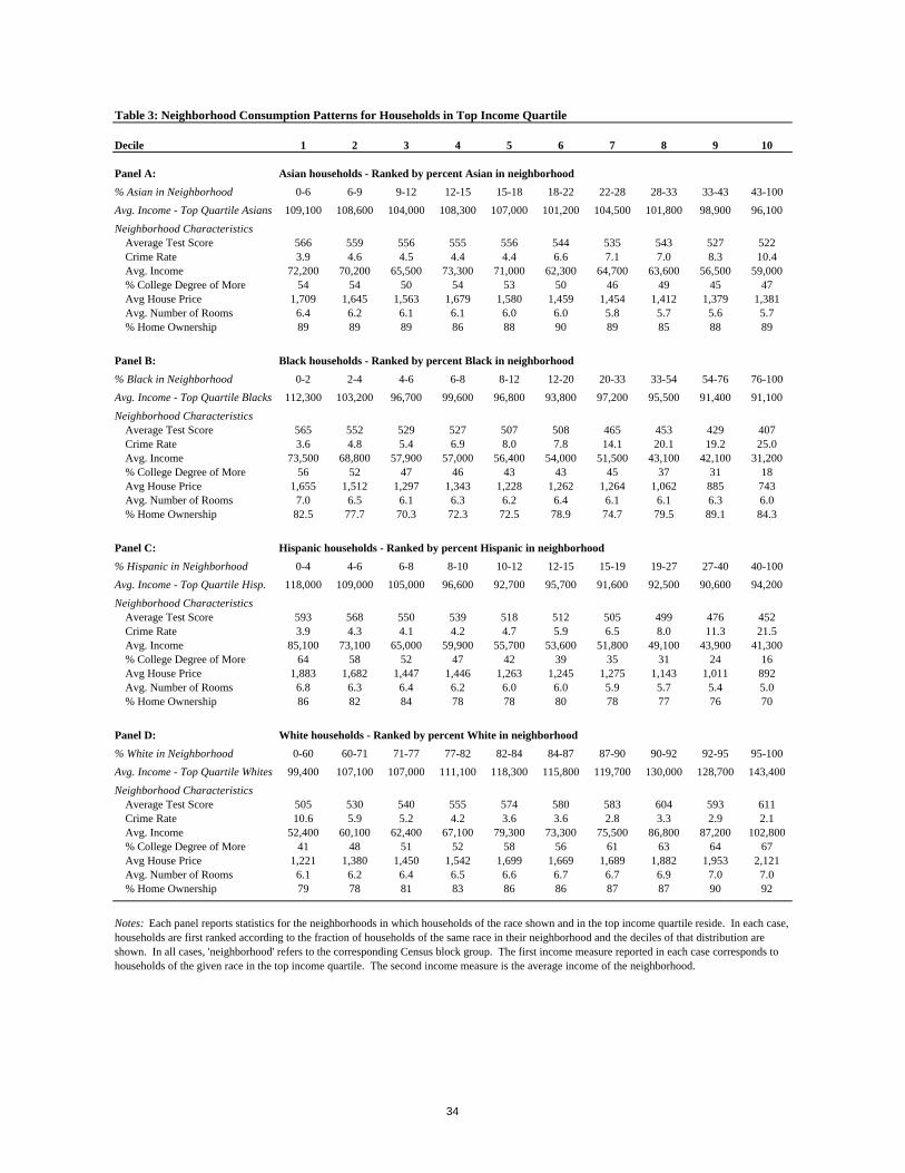
Table 3: Neighborhood Consumption Patterns for Households in Top Income Quartile

Decile 1 2 3 4 5 6 7 8 9 10

Panel A: Asian households - Ranked by percent Asian in neighborhood

% Asian in Neighborhood 0-6 6-9 9-12 12-15 15-18 18-22 22-28 28-33 33-43 43-100

Avg. Income - Top Quartile Asians 109,100 108,600 104,000 108,300 107,000 101,200 104,500 101,800 98,900 96,100

Neighborhood CharacteristicsAverage Test Score 566 559 556 555 556 544 535 543 527 522Crime Rate 3.9 4.6 4.5 4.4 4.4 6.6 7.1 7.0 8.3 10.4Avg. Income 72,200 70,200 65,500 73,300 71,000 62,300 64,700 63,600 56,500 59,000% College Degree of More 54 54 50 54 53 50 46 49 45 47Avg House Price 1,709 1,645 1,563 1,679 1,580 1,459 1,454 1,412 1,379 1,381Avg. Number of Rooms 6.4 6.2 6.1 6.1 6.0 6.0 5.8 5.7 5.6 5.7% Home Ownership 89 89 89 86 88 90 89 85 88 89

Panel B: Black households - Ranked by percent Black in neighborhood

% Black in Neighborhood 0-2 2-4 4-6 6-8 8-12 12-20 20-33 33-54 54-76 76-100

Avg. Income - Top Quartile Blacks 112,300 103,200 96,700 99,600 96,800 93,800 97,200 95,500 91,400 91,100

Neighborhood CharacteristicsAverage Test Score 565 552 529 527 507 508 465 453 429 407Crime Rate 3.6 4.8 5.4 6.9 8.0 7.8 14.1 20.1 19.2 25.0Avg. Income 73,500 68,800 57,900 57,000 56,400 54,000 51,500 43,100 42,100 31,200% College Degree of More 56 52 47 46 43 43 45 37 31 18Avg House Price 1,655 1,512 1,297 1,343 1,228 1,262 1,264 1,062 885 743Avg. Number of Rooms 7.0 6.5 6.1 6.3 6.2 6.4 6.1 6.1 6.3 6.0% Home Ownership 82.5 77.7 70.3 72.3 72.5 78.9 74.7 79.5 89.1 84.3

Panel C: Hispanic households - Ranked by percent Hispanic in neighborhood

% Hispanic in Neighborhood 0-4 4-6 6-8 8-10 10-12 12-15 15-19 19-27 27-40 40-100

Avg. Income - Top Quartile Hisp. 118,000 109,000 105,000 96,600 92,700 95,700 91,600 92,500 90,600 94,200

Neighborhood CharacteristicsAverage Test Score 593 568 550 539 518 512 505 499 476 452Crime Rate 3.9 4.3 4.1 4.2 4.7 5.9 6.5 8.0 11.3 21.5Avg. Income 85,100 73,100 65,000 59,900 55,700 53,600 51,800 49,100 43,900 41,300% College Degree of More 64 58 52 47 42 39 35 31 24 16Avg House Price 1,883 1,682 1,447 1,446 1,263 1,245 1,275 1,143 1,011 892Avg. Number of Rooms 6.8 6.3 6.4 6.2 6.0 6.0 5.9 5.7 5.4 5.0% Home Ownership 86 82 84 78 78 80 78 77 76 70

Panel D: White households - Ranked by percent White in neighborhood

% White in Neighborhood 0-60 60-71 71-77 77-82 82-84 84-87 87-90 90-92 92-95 95-100

Avg. Income - Top Quartile Whites 99,400 107,100 107,000 111,100 118,300 115,800 119,700 130,000 128,700 143,400

Neighborhood CharacteristicsAverage Test Score 505 530 540 555 574 580 583 604 593 611Crime Rate 10.6 5.9 5.2 4.2 3.6 3.6 2.8 3.3 2.9 2.1Avg. Income 52,400 60,100 62,400 67,100 79,300 73,300 75,500 86,800 87,200 102,800% College Degree of More 41 48 51 52 58 56 61 63 64 67Avg House Price 1,221 1,380 1,450 1,542 1,699 1,669 1,689 1,882 1,953 2,121Avg. Number of Rooms 6.1 6.2 6.4 6.5 6.6 6.7 6.7 6.9 7.0 7.0% Home Ownership 79 78 81 83 86 86 87 87 90 92

Notes: Each panel reports statistics for the neighborhoods in which households of the race shown and in the top income quartile reside. In each case, households are first ranked according to the fraction of households of the same race in their neighborhood and the deciles of that distribution are shown. In all cases, 'neighborhood' refers to the corresponding Census block group. The first income measure reported in each case corresponds to households of the given race in the top income quartile. The second income measure is the average income of the neighborhood.

34

Table 4: Neighborhood Consumption Patterns for Households in Bottom Income Quartile

Decile 1 2 3 4 5 6 7 8 9 10

Panel A: Asian households - Ranked by Percent Asian in neighborhood

% Asian in Neighborhood 0-6.5 6.5-10 10-14 14-17 17-21 21-27 27-32 32-40 40-66 67-100

Avg. Income - Bottom Quart. Asians 12,600 12,300 11,900 12,200 12,200 12,400 12,000 12,600 12,300 10,400

Neighborhood CharacteristicsAverage Test Score 505 502 498 501 495 497 506 504 493 467Crime Rate 9.9 11.5 11.0 13.4 17.4 20.2 19.5 16.9 22.6 38.0Avg. Income 44,600 44,600 41,700 43,000 39,300 37,300 36,300 39,000 40,200 23,000% College Degree of More 38 39 39 42 40 35 38 39 35 16Avg House Price 770 754 720 733 690 679 619 698 710 389Avg. Number of Rooms 3.7 3.5 3.4 3.4 3.3 3.2 3.0 3.4 3.5 2.1% Home Ownership 34 29 27 29 25 30 20 24 31 5

Panel B: Black households - Ranked by Percent Black in neighborhood

% Black in Neighborhood 0-7 7-14 14-26 26-37 37-49 49-65 65-74 74-82 82-88 88-100

Avg. Income - Bottom Quart. Blacks 12,900 12,200 12,100 11,400 11,800 11,400 109,000 11,100 10,300 10,500

Neighborhood CharacteristicsAverage Test Score 516 488 466 458 436 443 429 404 409 387Crime Rate 10.8 15.0 18.5 20.6 23.9 21.6 25.5 23.8 30.9 27.4Avg. Income 45,200 39,500 34,700 33,200 30,200 28,900 26,500 25,900 23,100 23,100% College Degree of More 42 35 35 34 26 22 20 16 12 12Avg House Price 722 667 601 524 504 498 474 471 446 432Avg. Number of Rooms 3.7 3.7 3.7 3.8 3.6 4.0 4.2 4.1 4.2 4.3% Home Ownership 19 22 19 21 20 31 34 33 29 35

Panel C: Hispanic households - Ranked by Percent Hispanic in neighborhood

% Hispanic in Neighborhood 0-6 6-9 9-12 12-15 15-20 20-28 28-33 33-43 43-57 57-100

Avg. Income - Bottom Quart. Hisp 13,200 13,100 13,200 13,800 13,400 13,500 13,400 13,000 13,200 13,000

Neighborhood CharacteristicsAverage Test Score 526 513 502 495 484 470 458 456 445 441Crime Rate 12.3 11.3 10.0 8.5 10.3 10.9 13.3 15.4 23.1 23.3Avg. Income 47,800 41,600 41,300 41,400 40,400 36,900 36,400 34,700 34,700 32,600% College Degree of More 48 41 35 34 31 26 24 20 18 11Avg House Price 736 700 669 678 670 620 614 597 600 629Avg. Number of Rooms 3.7 3.7 3.8 3.7 3.8 3.6 3.5 3.6 3.4 3.5% Home Ownership 30 25 28 31 34 24 26 23 20 23

Panel D: White households - Ranked by Percent White in neighborhood

% White in Neighborhood 0-44.5 44.5-57 57-65 65-71 71-76 76-80 80-84 84-88 88-92 92-100

Avg. Income - Bottom Quart.A55 Whites12,500 12,800 13,100 13,700 13,600 13,500 13,800 13,600 13,700 13,500

Neighborhood CharacteristicsAverage Test Score 454 492 499 502 511 524 539 543 572 576Crime Rate 20.5 15.1 12.4 10.4 8.5 5.0 5.0 4.0 4.3 2.6Avg. Income 33,700 36,500 38,900 42,300 44,700 47,400 51,200 51,200 62,100 64,100% College Degree of More 24 35 37 40 42 42 44 44 53 52Avg House Price 609 648 664 724 757 820 883 838 987 1034Avg. Number of Rooms 3.9 3.7 3.8 3.9 4.0 4.3 4.4 4.3 4.6 4.7% Home Ownership 40 34 36 39 41 43 48 48 54 66

Notes: Each panel reports statistics for the neighborhoods in which households of the race shown and in the bottom income quartile reside. In each case, households are first ranked according to the fraction of households of the same race in their neighborhood and the deciles of that distribution are shown. In all cases, 'neighborhood' refers to the corresponding Census block group. The first income measure reported in each case corresponds to households of the given race in the bottom income quartile. The second income measure is the average income of the neighborhood.

35

Table 5: Implied Mean MWTP Measures

Sample

Boundary Fized Effects

Observations

% Black*

% Hispanic*

% Asian*

% College Degree or More

Average Income*

Average Test Score (in s.d.'s)

Owner-Occupied

Number of Rooms

Built in 1980s

Built in 1960s or 1970s

Elevation (/100)

Population Density

Crime Index

F-statistic for boundary fixed effects

(3)(1)

Notes: All neighborhood attributes are measured using the corresponding Census block group. Specifications shown in the table also include controls for interactions between neighborhood racial composition variables and average income as well as land use (% industrial, % residential, % commercial, % open space, % other) in 1, 2, 3, 4, and 5 mile rings around location and six variables that characterize the housing stock in each of these rings. *Coefficients for % Asian,% Black, % Hispanic, Average Income reported at mean.

4.162

(38.87)

104.11

(59.01)

23.12

(17.31)

-1.02

No Yes

85.44(2.64)

149.77

(55.21)

164.78

(39.42)

(2)

-233.94

(1.60)

21.46

(5.29)

6.15

(3.99)

87.40

(10.00)

2.48

(7.47)

148.15

-0.49

(2.18)

40.88

(13.87)

(6.86)

71.36

111.67

(1.95)

(7.38)

109.28

(1.96)

1.32

(0.65)

-285.46

(32.06)

-37.19

(46.83)

-69.84

(45.68)

185.74

(25.96)

-14.57

18.40

(1.53)

154.93

16.69

(4.23)

(11.40)

249.63

(9.19)

(9.29)

83.15(0.74)

141.08

(7.40)

89.48(2.18)

(9.80)

-9.72

(13.59)

-48.97

20.16

(3.23)

-0.39(0.16)

-1.70

(0.68)

99.60

(3.36)

20.52

(2.41)

(2.66)

111.71

(0.69)

within .25 mile of boundaries

27,958 27,958242,100

No

full sample

-316.00

Residential Sorting Model

(0.18)

(3.56)

0.38

(2.93)

122.29

35.86

(3.69)

15.98

(2.65)

(0.76)

27,958

within .25 mile of boundaries

Hedonic Price Regressions

(4.39)

(1) (2)

full sample

27,958242,100

6.51

(3)

14.65

(2.16)

108.57

(10.99)

(19.04)

0.36(1.76)

No No Yes

-40.46

(42.74)

254.31

(64.88)

8.754

109.22(2.90)

241.13

4.87

(8.21)

(60.71)

177.11

(43.34)

121.72

113.26(2.40)

125.63

(8.12)

19.01

(4.66)

117.59

(8.14)

23.67

(5.81)

-1.69

(50.27)

235.04

(28.57)

-94.96

(35.28)

106.60

(51.54)

49.13

(15.27)

0.94(0.71)

-14.08

(2.40)

1.75

(0.75)

-101.92

(10.78)

142.64

(1.68)

(14.95)

67.84

(12.54)

303.16

(10.11)

107.98

101.88

24.19

(0.82)

133.56

-4.40

(7.55)

123.91

(2.15)

80.58

(10.23)

36

Table 6. Heterogeneity in Marginal Willingness to Pay for Selected Neighborhood and Housing Attributes

+10% Asian +10% Black +10% Hisp +10% College Blk Group Own vs. Rent +1 Room Built in 1980svs. White vs. White vs. White Educated Avg Income vs. pre-1960(at mean) (at mean) (at mean) + $10,000

Mean MWTP 10.4 -23.4 15.0 16.5 85.4 148.2 109.3 87.4

(5.9) (3.9) (5.5) (3.9) (2.6) (7.4) (2.0) (10.0)

Race (at mean income=$54,755)Asian 97.9 -10.5 25.0 10.3 86.9 253.3 78.8 118.3Black 38.5 66.6 44.1 35.9 65.8 80.3 117.4 96.9Hispanic 8.7 -9.3 71.1 17.5 91.0 130.7 96.8 73.9White -8.1 -37.8 1.1 14.8 86.5 139.5 115.8 82.9

Race (at income=$120,000)Asian 83.2 -31.7 -0.1 18.4 100.2 394.1 120.2 182.1Black 37.5 28.6 19.0 41.3 79.2 221.4 159.0 160.8Hispanic 7.7 -30.6 64.4 22.9 107.1 276.4 141.9 140.5White -9.1 -58.9 -23.9 20.1 98.0 277.2 155.0 144.9

Educationless than college degree 15.6 -26.0 17.4 -9.1 87.5 134.5 107.0 69.8college degree 3.8 -20.1 11.9 49.4 82.7 165.6 112.2 110.0

House CharacteristicsNeighborhood Sociodemographics

Notes: All figures are estimates of marginal wilingness to pay for the change shown in the column heading. Figures are reported in terms of a monthly rent - see Data Appendix for a discussion of corresponding price is created for owner-occupied housing units in the sample. The first row of the table reports the

in the row heading and mean attributes for all other characteristics. All estimates are based on specification that includes boundary fixed effects and all neighborhood variables are measured using the corresponding Census block group.

37

Table 7: Counterfactual - Eliminating Racial Interactions in Location Decision: Exposure Rates

Panel A: Pre-ExperimentAsian Black Hispanic White

Asian 0.233 0.072 0.115 0.573Black 0.118 0.384 0.113 0.377Hispanic 0.130 0.078 0.218 0.558White 0.103 0.042 0.089 0.760

Panel B: General Equilibrium - UnadjustedAsian Black Hispanic White

Asian 0.111 0.067 0.114 0.700Black 0.110 0.147 0.088 0.646Hispanic 0.129 0.061 0.105 0.690White 0.126 0.071 0.110 0.687

Panel C: General Equilibrium - AdjustedAsian Black Hispanic White

Asian 0.111 0.068 0.114 0.700Black 0.110 0.146 0.089 0.645Hispanic 0.129 0.062 0.104 0.690White 0.126 0.071 0.110 0.687

Note: Each entry in the table shows the average exposure of households of the race shown in the row heading tohouseholds of the race shown in the column heading. Figures are reported for a counterfactual simulation that setsall preference parameters associated with neighborhood racial composition to zero.

38

Table 8: Counterfactual - Eliminating Racial Interactions in Location Decision: Consumption Measures

Asian Black Hispanic White

Pre-Experiment 0.64 0.40 0.46 0.63General Equilibrium - Unadjusted 0.67 0.35 0.46 0.63General Equilibrium - Adjusted 0.67 0.35 0.46 0.63

Pre-Experiment 4.68 4.50 4.49 5.36General Equilibrium - Unadjusted 4.76 4.53 4.67 5.31General Equilibrium - Adjusted 4.76 4.53 4.67 5.31

Pre-Experiment 521 458 491 541General Equilibrium - Unadjusted 528 502 514 531General Equilibrium - Adjusted 529 496 515 531

Pre-Experiment 10.33 18.73 11.50 6.14General Equilibrium - Unadjusted 8.04 12.11 8.65 7.75General Equilibrium - Adjusted 7.89 13.01 8.58 7.71

Pre-Experiment 1092 740 882 1160General Equilibrium - Unadjusted 1134 868 962 1126General Equilibrium - Adjusted 1138 846 964 1127

Pre-Experiment 10.17 9.89 11.07 10.28General Equilibrium - Unadjusted 10.23 9.15 10.22 9.86General Equilibrium - Adjusted 10.28 9.05 10.24 9.88

Pre-Experiment 52,551 37,377 44,622 57,624General Equilibrium - Unadjusted 54,364 44,711 49,814 55,665General Equilibrium - Adjusted 54,381 44,356 49,848 55,696

Pre-Experiment 0.43 0.31 0.31 0.47General Equilibrium - Unadjusted 0.44 0.38 0.38 0.45General Equilibrium - Adjusted 0.44 0.37 0.38 0.45

Note: This table reports the consumption of housing and local public goods by households of each race.Numbers are reported for a counterfactual simulation that sets all preference parameters associated withneighborhood racial composition to zero.

Percent College Educated

Average Neighborhood Income

House Size

Ownership Rates

Average Commutes

Average House Rental Value

Average Crime Rates

Average Math Scores

39

Table 9: Counterfactual - Eliminating Racial Interactions in Location Decision: Consumption Measures by Race and Income

Bottom Income Quartile Top Income QuartileAsian Black Hispanic White Asian Black Hispanic White

Pre-Experiment 0.42 0.31 0.31 0.46 0.89 0.72 0.78 0.87General Equilibrium - Unadjusted 0.45 0.22 0.28 0.45 0.91 0.76 0.83 0.87General Equilibrium - Adjusted 0.45 0.22 0.28 0.45 0.91 0.76 0.83 0.87

Pre-Experiment 3.62 4.08 3.85 4.36 5.95 5.96 5.84 6.56General Equilibrium - Unadjusted 3.67 3.94 3.87 4.31 6.07 6.27 6.24 6.50General Equilibrium - Adjusted 3.67 3.94 3.87 4.30 6.07 6.26 6.25 6.51

Pre-Experiment 499 445 479 521 547 502 519 565General Equilibrium - Unadjusted 505 490 498 508 556 535 548 559General Equilibrium - Adjusted 505 482 498 506 557 533 549 559

Pre-Experiment 15.09 21.29 13.45 8.42 5.96 11.53 8.16 4.18General Equilibrium - Unadjusted 11.13 14.06 10.92 10.78 4.93 6.98 5.24 5.03General Equilibrium - Adjusted 11.11 15.30 11.03 10.95 4.78 7.29 5.09 4.93

Pre-Experiment 753 612 695 838 1,580 1,261 1,408 1,607General Equilibrium - Unadjusted 742 689 698 788 1,678 1,490 1,632 1,585General Equilibrium - Adjusted 743 661 696 786 1,683 1,477 1,636 1,586

Pre-Experiment 9.59 9.76 11.49 9.88 11.06 10.00 11.37 11.16General Equilibrium - Unadjusted 9.72 8.94 10.42 9.46 11.09 10.09 11.13 10.71General Equilibrium - Adjusted 9.76 8.82 10.42 9.47 11.15 10.02 11.18 10.73

Pre-Experiment 41,823 33,093 39,587 46,710 66,603 53,053 57,669 71,805General Equilibrium - Unadjusted 43,754 39,858 42,645 44,893 68,061 60,295 66,433 69,319General Equilibrium - Adjusted 43,662 39,258 42,494 44,732 68,084 60,365 66,567 69,387

Pre-Experiment 0.35 0.28 0.28 0.40 0.51 0.43 0.40 0.56General Equilibrium - Unadjusted 0.36 0.34 0.33 0.37 0.53 0.50 0.50 0.55General Equilibrium - Adjusted 0.36 0.32 0.33 0.36 0.53 0.50 0.50 0.55

Note: This table reports the consumption of housing and neighborhood amenities by households of each race in the bottom and top quartile of the overall incomedistribution, respectively. Numbers are reported for a counterfactual simulation that sets all preference parameters associated with neighborhood racial compositionto zero.

Average Monthly Rental Value

Ownership Rates

House Size

Average Test Score

Average Crime Rate

Percent College Educated Percent College Educated

Average Neighborhood Income

Average Commute

Average Neighborhood Income

Average Commute

Ownership Rates

Average Monthly Rental Value

Average Crime Rate

Average Test Score

House Size

40

Table 10: Counterfactual - Equalizing Income and Wealth Across Race: Exposure Rates

Panel A: Pre-Experiment Asian Black Hispanic White

Asian 0.233 0.072 0.115 0.573Black 0.118 0.384 0.113 0.377Hispanic 0.130 0.078 0.218 0.558White 0.103 0.042 0.089 0.760

Panel B: Partial EquilibriumAsian Black Hispanic White

Asian 0.228 0.076 0.116 0.573Black 0.123 0.342 0.100 0.426Hispanic 0.131 0.069 0.194 0.590White 0.103 0.047 0.094 0.749

Panel C: General Equilibrium - UnadjustedAsian Black Hispanic White

Asian 0.251 0.070 0.089 0.584Black 0.115 0.355 0.100 0.422Hispanic 0.100 0.069 0.229 0.586White 0.105 0.047 0.094 0.749

Panel D: General Equilibrium - AdjustedAsian Black Hispanic White

Asian 0.255 0.070 0.088 0.580Black 0.115 0.367 0.103 0.407Hispanic 0.099 0.071 0.237 0.577White 0.104 0.045 0.092 0.752

Note: Each entry in the table shows the average exposure of households of the race shown in the rowheading to households of the race shown in the column heading. Numbers are reported for a counterfactualsimulation that eliminates racial differences in income and wealth by replacing the income and wealth ofthe household in the p-th percentile of the income distribution within its own race with the income andwealth of the household in the p-th percentile of the overall income distribution.

41

Table 11: Counterfactual - Equalizing Income and Wealth Across Race: Consumption Measures

Bottom Income Quartile Top Income QuartileAsian Black Hispanic White Asian Black Hispanic White

Pre-Experiment 0.42 0.31 0.31 0.46 0.89 0.72 0.78 0.87General Equilibrium - Unadjusted 0.59 0.50 0.45 0.43 0.90 0.89 0.88 0.83General Equilibrium - Adjusted 0.63 0.49 0.45 0.42 0.90 0.89 0.88 0.84

Pre-Experiment 3.62 4.08 3.85 4.36 5.95 5.96 5.84 6.56General Equilibrium - Unadjusted 3.88 4.44 4.01 4.32 5.99 6.79 6.53 6.32General Equilibrium - Adjusted 3.84 4.34 3.94 4.31 6.02 6.79 6.52 6.36

Pre-Experiment 499 445 479 521 547 502 519 565General Equilibrium - Unadjusted 506 453 484 519 549 533 542 557General Equilibrium - Adjusted 504 449 480 518 550 533 541 559

Pre-Experiment 15.09 21.29 13.45 8.42 5.96 11.53 8.16 4.18General Equilibrium - Unadjusted 11.74 18.91 12.39 9.19 5.55 7.89 5.88 5.03General Equilibrium - Adjusted 12.38 19.99 13.05 9.16 5.43 7.93 5.99 4.71

Pre-Experiment 753 612 695 838 1,580 1,261 1,408 1,607General Equilibrium - Unadjusted 770 798 784 788 1,561 1,580 1,550 1,555General Equilibrium - Adjusted 771 783 776 789 1,567 1,563 1,556 1,556

Pre-Experiment 9.59 9.76 11.49 9.88 11.06 10.00 11.37 11.16General Equilibrium - Unadjusted 10.01 9.83 11.21 9.80 11.34 11.03 12.03 10.64General Equilibrium - Adjusted 9.92 9.70 11.22 9.80 11.37 11.02 11.99 10.67

Pre-Experiment 41,823 33,093 39,587 46,710 66,603 53,053 57,669 71,805General Equilibrium - Unadjusted 46,916 38,212 43,040 47,613 66,621 55,194 60,229 66,229General Equilibrium - Adjusted 46,689 38,177 42,405 47,241 67,162 55,765 60,561 66,615

Pre-Experiment 0.35 0.28 0.28 0.40 0.51 0.43 0.40 0.56General Equilibrium - Unadjusted 0.37 0.27 0.29 0.41 0.49 0.43 0.40 0.53General Equilibrium - Adjusted 0.42 0.34 0.33 0.47 0.49 0.43 0.41 0.54

Ownership Rates

Average Neighborhood Income

Ownership Rates

House Size

Average Math Scores

Average Crime Rates

Average Commutes

Average Neighborhood Income

Average Commutes

Average Monthly Rental Value

Note: This table reports the consumption of housing and neighborhood amenities by households of each race in the bottom and top quartile of the overall income distribution, respectively. Numbers are reported for a counterfactual simulation that eliminates racial differences in income and wealth by replacing the income and wealth of the household in the p-th percentile of the income distribution within its own race with the income and wealth of the household in the p-th percentile of the overall income distribution.

Percent College Educated

House Size

Average Math Scores

Average Crime Rates

Percent College Educated

Average Monthly Rental Value

42

Table 12: Number of Tracts in United States in 2000 by Race and Education

Percent College Degree or Moreat least

Percent Black 0% 20% 40% 60% 80%at least 0%

Number 49,021 26,351 11,094 3,005 203Fraction of tracts at least 0% black 100.0% 53.8% 22.6% 6.1% 0.4%

at least 20%Number 9,149 2,567 641 59 0Fraction of tracts at least 20% black 100.0% 28.1% 7.0% 0.6% 0.0%

at least 40%Number 5,657 1,164 142 14 0Fraction of tracts at least 40% black 100.0% 20.6% 2.5% 0.2% 0.0%

at least 60%Number 3,921 623 44 5 0Fraction of tracts at least 60% black 100.0% 15.9% 1.1% 0.1% 0.0%

at least 80%Number 2,559 271 21 1 0Fraction of tracts at least 80% black 100.0% 10.6% 0.8% 0.0% 0.0%

PMSA Locations of Tracts AveragePercentage black >80% >60% >40% Percent Black-BlackPercentage w/ college degree >40% >40% >40% Black Exposure*

Washington, DC 5 13 29 25% 58%Detroit, MI 5 8 17 21% 78%Chicago, IL 3 16 17% 72%New York, NY 4 12 23% 61%Los Angeles, CA 4 6 10 10% 38%Atlanta, GA 5 5 8 26% 60%Cleveland, OH 1 6 16% 70%Philadelphia, PA 1 5 18% 62%Oakland, CA 5 12% 35%Baltimore, MD 4 25% 64%Raleigh-Durham, NC 1 3 12% 31%Indianapolis, IN 3 12% 51%Newark, NJ 3 20% 66%Jackson, MS 1 1 2 25% 58%Houston, TX 1 1 2 17% 48%Columbia, SC 2 17% 43%Ann Arbor, MI 2 7% 27%New Orleans, LA 2 33% 67%

Total 21 44 142

Notes: Tracts considered have a minimum of 800 households (the average tract in the US has almost 3,000 households) Exposure measures reported in fifth column of lower panel are the average fraction of black households in the Census tracts in which black households reside.

43

Table 13: Segregation Across Metropolitan Areas

Sample:

Dependent Variable:

Any College Degree Less than College Any College Degree Less than College Any College Degree Less than College

Fraction PMSA - Black w/ Col. Deg. (β1) 1.43 1.93 1.90 2.21 2.40 2.69 3.75** 3.23** 4.20***(1.12) (0.81) (1.16) (1.18) (0.95) (1.22) (1.35) (1.10) (1.39)

Fraction PMSA - Black w/out Col. Deg. (β2) 1.98*** 1.62*** 1.95*** 0.97 1.00 0.90 0.39** 0.53* 0.31**(0.18) (0.13) (0.18) (0.21) (0.17) (0.21) (0.29) (0.24) (0.30)

Test: β1-β2=0 ++ ++ ++

Sample:

Dependent Variable:

Any College Degree Less than College Any College Degree Less than College Any College Degree Less than College

Fraction PMSA - Asian w/ Col. Deg. (β1) 3.11*** 3.55*** 2.34*** 2.95*** 3.37*** 2.24*** 2.78*** 3.11*** 2.20***(0.15) (0.16) (0.13) (0.21) (0.21) (0.19) (0.30) (0.31) (0.28)

Fraction PMSA - Asian w/out Col. Deg. (β2) 0.80 0.24*** 1.50*** 0.74 0.19*** 1.46*** 0.56* 0.06*** 1.28(0.13) (0.13) (0.11) (0.17) (0.18) (0.15) (0.25) (0.25) (0.23)

Test: β1-β2=0 +++ +++ +++ +++ +++ ++ +++ +++ ++

Sample:

Dependent Variable:

Any College Degree Less than College Any College Degree Less than College Any College Degree Less than College

Fraction PMSA - Hispanic w/ Col. Deg. (β1) -0.65*** 1.49** -0.55*** -0.46** 1.54* -0.35* 0.03 1.74** 0.17(0.51) (0.24) (0.55) (0.60) (0.31) (0.64) (0.61) (0.36) (0.65)

Fraction PMSA - Hispanic w/out Col. Deg. (β2) 1.40*** 0.92*** 1.41*** 1.22*** 0.86*** 1.22*** 1.06 0.81*** 1.05(0.06) (0.03) (0.06) (0.07) (0.04) (0.08) (0.08) (0.05) (0.08)

Test: β1-β2=0 --- ++ --- -- ++ -- ++

Own-Race Exposure of Hispanic Hhlds w/ Education Own-Race Exposure of Hispanic Hhlds w/ Education Own-Race Exposure of Hispanic Hhlds w/ Education

Own-Race Exposure of Asian Hhlds with Education Own-Race Exposure of Asian Hhlds with Education Own-Race Exposure of Asian Hhlds with Education

% Hispanic > 0% in PMSA (n=330) % Hispanic > 3.2% in PMSA (n=165) % Hispanic > 6.4% in PMSA (n=103)

Note: This table reports the results of 27 regressions that relate various average exposure rates at the PMSA level to variables that characterize the sociodemographic characteristics of the PMSA's population. Results arereported separately for Black, Asian, and Hispanic households. For each race results are reported for the own-race exposure of all households and households with and without a college degree, respectively. Results arereported for (i) all PMSAs; (ii) PMSAs with the fraction of each race above the median fraction for all PMSAs in the US; (iii) PMSAs with the fraction of each race above twice the median fraction. Standard errors are inparentheses. ***, **, * denote that the coefficient is statistically different from 1.0 at 1%, 5%, and 10% confidence levels, respectively. +++,++,+ denotes that difference is positive and statistically significant at 1%,5%,and 10% confidence levels, respectively. ---,--,- denotes that difference is negative and statistically significant at 1%,5%, and 10% confidence levels, respectively.

% Black > 0% in PMSA (n=330) % Black > 6.2% in PMSA (n=165) % Black > 12.5% in PMSA (n=77)

Own-Race Exposure of Black Hhlds with Education

% Asian > 0% in PMSA (n=330) % Asian > 1.4% in PMSA (n=165) % Black > 2.8% in PMSA (n=69)

Own-Race Exposure of Black Hhlds with Education Own-Race Exposure of Black Hhlds with Education

44

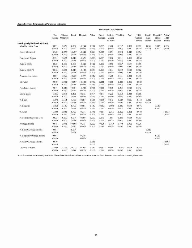
Appendix Table 1: Interaction Parameter Estimates

Hhld Children Black Hispanic Asian Some College Working Age Hhld Black* Hispanic* Asian*Income Under 18 College Degree Capital Hhld Hhld Hhld

or More Income Income Income IncomeHousing/Neighborhood Attribute

Monthly House Price 0.071 0.071 0.087 -0.244 0.208 0.285 0.400 0.197 0.007 0.013 0.030 0.082 0.034(0.003) (0.023) (0.051) (0.048) (0.056) (0.068) (0.042) (0.062) (0.001) (0.002) (0.015) (0.025) (0.013)

Owner-Occupied 0.142 -0.050 -0.427 -0.046 0.851 0.027 0.191 0.303 0.046 0.094(0.005) (0.025) (0.058) (0.036) (0.058) (0.051) (0.038) (0.065) (0.004) (0.007)

Number of Rooms 0.151 0.522 0.010 -0.521 -1.223 0.085 0.036 0.011 0.007 -0.060(0.005) (0.027) (0.034) (0.052) (0.071) (0.047) (0.031) (0.043) (0.001) (0.005)

Built in 1980s 0.045 -0.064 0.065 -0.040 0.184 0.192 0.196 0.337 -0.011 0.019(0.004) (0.021) (0.046) (0.030) (0.045) (0.062) (0.037) (0.068) (0.001) (0.003)

Built in 1960-79 0.013 0.023 0.315 -0.139 0.221 0.163 0.044 0.209 -0.005 0.002(0.003) (0.018) (0.054) (0.045) (0.057) (0.065) (0.029) (0.060) (0.001) (0.001)

Average Test Score 0.001 0.056 -0.229 -0.077 0.086 0.186 0.206 0.141 0.011 0.056(0.002) (0.023) (0.056) (0.039) (0.043) (0.066) (0.040) (0.057) (0.002) (0.002)

Elevation 0.019 0.038 -0.097 -0.134 0.006 0.141 0.090 -0.018 0.006 -0.039(0.002) (0.013) (0.038) (0.044) (0.036) (0.064) (0.036) (0.042) (0.001) (0.006)

Population Density 0.017 -0.216 -0.561 -0.030 0.004 -0.006 0.159 -0.253 -0.006 0.042(0.004) (0.024) (0.062) (0.031) (0.032) (0.036) (0.037) (0.063) (0.001) (0.005)

Crime Index -0.016 0.010 0.491 0.045 0.017 -0.044 0.235 -0.164 0.014 0.066(0.003) (0.021) (0.065) (0.038) (0.038) (0.044) (0.041) (0.059) (0.002) (0.010)

% Black -0.073 0.114 1.700 0.697 0.680 -0.089 0.145 -0.114 -0.003 -0.110 -0.032(0.005) (0.023) (0.069) (0.052) (0.060) (0.054) (0.037) (0.056) (0.001) (0.015) (0.019)

% Hispanic -0.063 0.125 0.700 0.891 0.425 -0.192 -0.094 -0.015 -0.010 -0.076 0.126(0.006) (0.019) (0.063) (0.055) (0.058) (0.062) (0.032) (0.043) (0.002) (0.012) (0.030)

% Asian -0.003 0.088 0.799 0.311 1.708 -0.064 -0.215 -0.056 0.001 -0.079 -0.036(0.005) (0.024) (0.061) (0.053) (0.063) (0.059) (0.040) (0.047) (0.001) (0.013) (0.021)

% College Degree or More 0.022 -0.200 0.574 0.080 -0.052 0.375 1.681 -0.338 -0.006 0.093(0.006) (0.025) (0.054) (0.047) (0.043) (0.070) (0.058) (0.065) (0.002) (0.014)

Average Income 0.045 0.048 -0.808 0.245 -0.053 -0.028 -0.313 0.100 0.003 0.020(0.006) (0.018) (0.057) (0.045) (0.041) (0.049) (0.053) (0.056) (0.001) (0.006)

% Black*Average Income 0.054 0.674 -0.026(0.009) (0.078) (0.032)

% Hispanic*Average Income 0.067 0.340 -0.081(0.010) (0.067) (0.039)

% Asian*Average Income 0.010 0.282 -0.003(0.009) (0.071) (0.027)

Distance to Work -0.022 0.156 -0.272 0.189 0.221 -0.093 0.160 -13.765 -0.010 -0.468(0.002) (0.023) (0.043) (0.035) (0.039) (0.058) (0.032) (0.056) (0.001) (0.019)

Household Characteristic

Note: Parameter estimates reported with all variables normalized to have mean zero, standard deviation one. Standard errors are in parentheses.

45