Embed Size (px)
Citation preview
HAL Id: hal-02910327https://hal.archives-ouvertes.fr/hal-02910327
Submitted on 1 Aug 2020
HAL is a multi-disciplinary open accessarchive for the deposit and dissemination of sci-entific research documents, whether they are pub-lished or not. The documents may come fromteaching and research institutions in France orabroad, or from public or private research centers.
L’archive ouverte pluridisciplinaire HAL, estdestinée au dépôt et à la diffusion de documentsscientifiques de niveau recherche, publiés ou non,émanant des établissements d’enseignement et derecherche français ou étrangers, des laboratoirespublics ou privés.
Reshaping diagrams for bending straightening of forgedaeronautical components
Ramiro Mena, Jose Vicente Aguado, Stéphane Guinard, Antonio Huerta
To cite this version:Ramiro Mena, Jose Vicente Aguado, Stéphane Guinard, Antonio Huerta. Reshaping diagrams forbending straightening of forged aeronautical components. International Journal of Advanced Manu-facturing Technology, Springer Verlag, inPress. hal-02910327
to appear in The International Journal of Advanced Manufacturing Technology(manuscript No. will be inserted by the editor)
Reshaping diagrams for bending straightening of forgedaeronautical components
Ramiro Mena1,2,3 · Jose V. Aguado2 · Stephane Guinard1 · Antonio
Huerta3,4
Received: date / Accepted: date
Abstract Large and thick-walled aluminium forgings
exhibit shape distortions induced by residual stresses.
To restore the nominal geometry, a series of highly-
manual and time-consuming reshaping operations need
to be carried out. In this paper, we are concerned with
the development of efficient computer simulation tools
to assist operators in bending straightening, which is
one of the most common reshaping operations. Our ap-
proach is based on the computation of reshaping di-
agrams, a tool that allows selecting a nearly optimal
bending load to be applied in order to minimize dis-
tortion. Most importantly, we show that the reshaping
diagram needs not to account for the residual stress
field, as its only effect is to shift of the reshaping di-
This project has received funding from the European Union’sHorizon 2020 research and innovation programme under theMarie Sk lodowska-Curie grant agreement No 675919.
Ramiro Menaramiro-francisco.mena-andrade@[email protected]
Jose V. [email protected]
Ste phane [email protected]
Antonio [email protected]
1 Airbus SAS, 18 rue Marius Terce, 31300 Toulouse, France.
2 Institut de Calcul Intensif (ICI) at Ecole Centrale deNantes, 1 rue de la Noe, 44300 Nantes, France.
3 Laboratori de Calcul Numeric (LaCaN). E.T.S. de Inge-nieros de Caminos, Canales y Puertos, Universitat Po-litecnica de Catalunya, Barcelona, Spain.
4 Centre Internacional de Metodes Numerics a l’Enginyeria(CIMNE), Barcelona, Spain
agram by some offset. That is, the overall behaviour
including a realistic 3D residual stress field in a forged
part can be retrieved by shifting the residual stress free
reshaping diagram by the appropriate offset. Finally,
we propose a strategy in order to identify the offset
on-the-fly during the reshaping operation using simple
force-displacement measures.
Keywords Residual Stresses · Shape distortion ·Bending straightening · Forged parts · Numerical
simulation · Reshaping diagrams
1 Introduction
Large and thick-walled aluminium forgings are widely
used as structural parts in the aeronautical industry.
The good formability of aluminium, together with its
great strength-to-weight ratio, allows producing com-
plex forged parts in an economical way [1]. Addition-
ally, when compared to other metal working processes,
such as extensive machining, welding or casting, im-
proved material properties in terms of grain size and
orientation are obtained [2].
Aluminium forgings undergo a multiple-step manu-
facturing process to produce the final aeronautical com-
ponent. We describe here a typical manufacturing se-
quence, although others are of course possible. First,
forged blanks are typically produced on hydraulic presses
with hot closed-dies [4]. The process continues with a
solution heat treatment (SHT) followed by quenching,
which is required to improve the mechanical proper-
ties of the material. As a counterpart, the quenching
step is the main responsible for the creation of residual
stresses due to the strong thermal gradients between the
surface and the core of the part. Bi-axial compression
stress state develops at the surface, counterbalanced by
2 R. Mena, J.V. Aguado, S. Guinard and A. Huerta
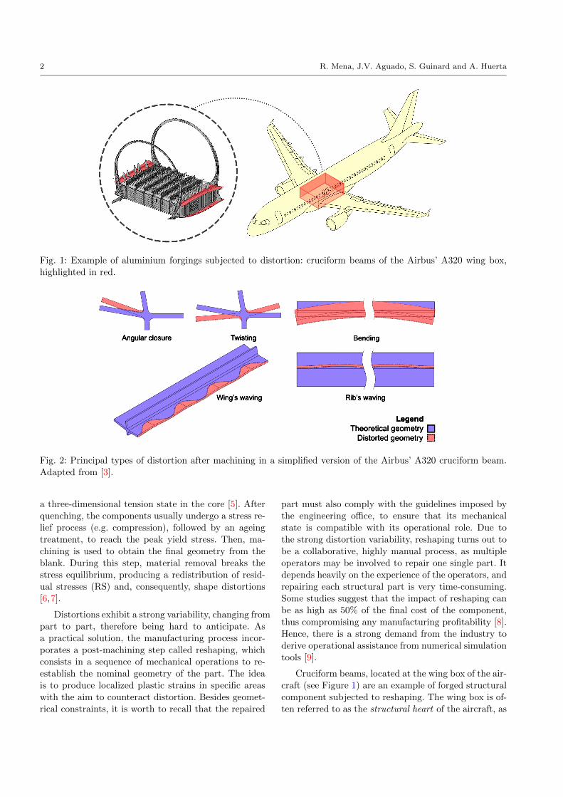
Fig. 1: Example of aluminium forgings subjected to distortion: cruciform beams of the Airbus’ A320 wing box,
highlighted in red.
Fig. 2: Principal types of distortion after machining in a simplified version of the Airbus’ A320 cruciform beam.
Adapted from [3].
a three-dimensional tension state in the core [5]. After
quenching, the components usually undergo a stress re-
lief process (e.g. compression), followed by an ageing
treatment, to reach the peak yield stress. Then, ma-
chining is used to obtain the final geometry from the
blank. During this step, material removal breaks the
stress equilibrium, producing a redistribution of resid-
ual stresses (RS) and, consequently, shape distortions
[6,7].
Distortions exhibit a strong variability, changing from
part to part, therefore being hard to anticipate. As
a practical solution, the manufacturing process incor-
porates a post-machining step called reshaping, which
consists in a sequence of mechanical operations to re-
establish the nominal geometry of the part. The idea
is to produce localized plastic strains in specific areas
with the aim to counteract distortion. Besides geomet-
rical constraints, it is worth to recall that the repaired
part must also comply with the guidelines imposed by
the engineering office, to ensure that its mechanical
state is compatible with its operational role. Due to
the strong distortion variability, reshaping turns out to
be a collaborative, highly manual process, as multiple
operators may be involved to repair one single part. It
depends heavily on the experience of the operators, and
repairing each structural part is very time-consuming.
Some studies suggest that the impact of reshaping can
be as high as 50% of the final cost of the component,
thus compromising any manufacturing profitability [8].
Hence, there is a strong demand from the industry to
derive operational assistance from numerical simulation
tools [9].
Cruciform beams, located at the wing box of the air-
craft (see Figure 1) are an example of forged structural
component subjected to reshaping. The wing box is of-
ten referred to as the structural heart of the aircraft, as
Reshaping diagrams for bending straightening of forged aeronautical components 3
it connects the wings to the fuselage and bears heavy
loads [10]. Being part of the wing box, cruciform beams
must meet tight dimensional tolerances to facilitate the
assembly process and to avoid undesired pre-loads in
such an important part of the aircraft.
Forged parts such as cruciform beams tend to de-
velop complex RS states, leading to complex distortion
patterns. Marin [3] documented the principal types of
distortions present on a cruciform as shown in Figure
2, where each type of distortion is represented indepen-
dently (although most often a combination of them is
observed).
Several reshaping operations can be found in the
literature to repair a distorted part. Among them, we
can cite the following: bending straightening [11,12],
torsion straightening [13,14], roller burnishing [15,16]
and ultrasonic needle peening [17,18]. While bending
and torsion create non-homogeneous deformation act-
ing along the whole cross-section, burnishing and peen-
ing induce local compressive residual stresses only at
the surface level. In this paper, we focus on the bend-
ing straightening operation only, which essentially con-
sists in applying a load in the opposite direction to ob-
served distortions. Bending straightening is an iterative
loading-unloading process, where, for a given initial dis-
tortion, the operator has to guess: i) where to place the
supports; ii) where to apply the bending load; and iii)
how much loading needs to be applied to minimize dis-
tortion.
Diverse authors have proposed to use numerical sim-
ulation as a means to anticipate the resulting shape af-
ter a correction step. The idea is that, from the knowl-
edge of the full residual state field prior to reshaping,
it should be possible to simulate the correction steps.
As residual stresses cannot be systematically measured
in an industrial context, lots of efforts have been de-
voted to derive numerical models that are able to es-
timate them [19,5]. These models require simulating,
either wholly or in part, the multi-step manufacturing
process. We shall refer to this approach throughout the
paper as the sequential approach, as depicted in Figure
3. Although the sequential approach can provide in-
sightful results when good knowledge on both process
conditions and material behaviour are available, most
often, significant mismatch between numerical predic-
tions and experimental observations is reported, e.g.
[20]. Assessing how uncertainties propagate through the
different manufacturing steps (i.e. from quenching to
machining) is key to keep a high confidence level on the
predictions from sequential models [7,21].
In this work, we deviate from the sequential ap-
proach and propose an alternative route to simulate
bending straightening of forged components. We first
introduce a simple tool, the reshaping diagram, which
provides the remaining distortion (i.e. after unloading)
as a function of the applied bending load (for fixed
rollers position and residual stress field). Note that the
reshaping diagram is a very convenient tool to assist
the operator: once it is made available, the reshap-
ing operation reduces to select the optimal bending
load that minimizes the remaining distortion. Unfor-
tunately, computing the reshaping diagram requires a
precise knowledge on the residual stress field, which
as discussed above, is not a trivial task. To overcome
this issue, we propose a workaround that uses distor-
tion (which is measurable) as the main input, instead
of residual stresses. The underlying idea is that to mini-
mize distortion we may not need a precise knowledge of
the residual stress field, but only its influence on the re-
shaping diagram. Therefore, we compute the reshaping
diagram of a distorted part without residual stresses,
that is, we keep the distorted geometry after machin-
ing but suppress the residual stress field. We shall refer
to this reshaping diagram throughout the entire paper
as the residual stress free (RSF) approach (see Figure
3). Then, we show that the effect of the RSF hypoth-
esis results only in a shift of the reshaping diagram.
That is, the overall behaviour including a realistic 3D
residual stress field in a forged part can be retrieved by
shifting the original reshaping diagram by the appro-
priate offset. Finally, we propose a strategy in order to
identify the offset on-the-fly during the reshaping op-
eration using simple force-displacement measures. One
of the main advantages of the RSF approach is that
it does not require any prior knowledge on the resid-
ual stress field; it only requires information on the dis-
torted shape, which unlike the residual stresses, can be
systematically measured in an industrial environment.
The rest of the paper is organized as follows. In sec-
tion 2, we present numerical models for residual stress
prediction and bending straightening simulation, and
validate them against available data in the literature.
Using the validated models, in section 3 we create real-
istic 3D stress states for forged parts and compute the
reference reshaping diagram by simulating the bending
straightening process. The influence of various process
parameters is also analysed. In section 4, we repeat the
operation with the residual stress free hypothesis and
observe that the obtained RSF reshaping diagram dif-
fers only by some offset from the reference one. In ad-
dition, we derive a simple approach to calibrate the
offset on-the-fly during the reshaping operation using
simple force-displacement measures. Finally, in section
5, we draw some conclusions and perspectives for future
work.
4 R. Mena, J.V. Aguado, S. Guinard and A. Huerta
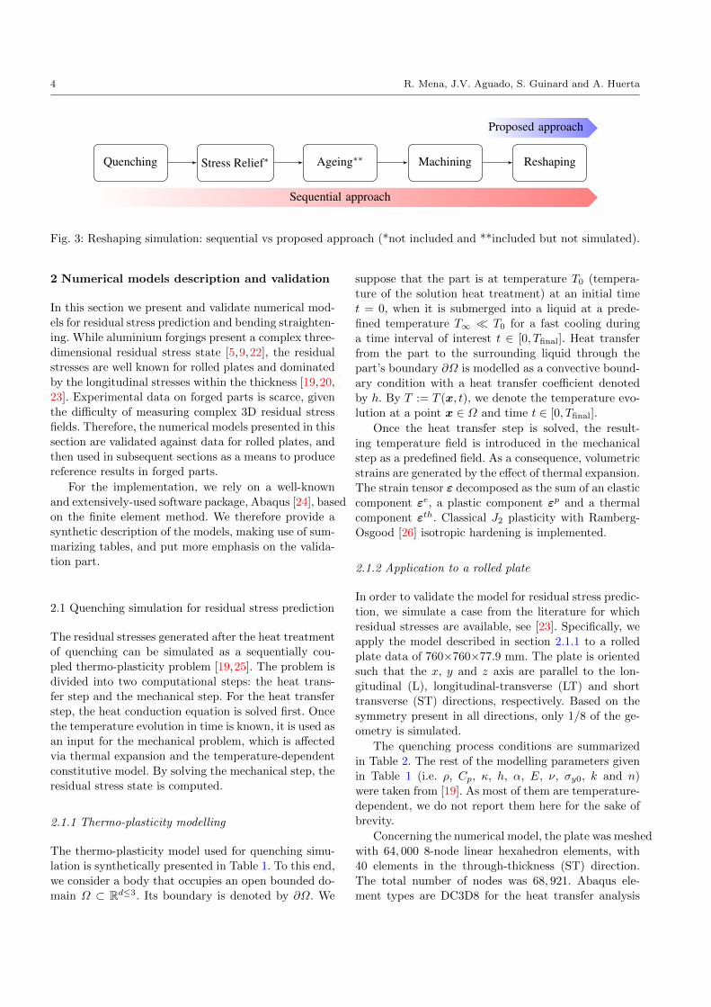
Quenching Stress Relief∗ Ageing∗∗ Machining Reshaping
Sequential approach
Proposed approach
Fig. 3: Reshaping simulation: sequential vs proposed approach (*not included and **included but not simulated).
2 Numerical models description and validation
In this section we present and validate numerical mod-
els for residual stress prediction and bending straighten-
ing. While aluminium forgings present a complex three-
dimensional residual stress state [5,9,22], the residual
stresses are well known for rolled plates and dominated
by the longitudinal stresses within the thickness [19,20,
23]. Experimental data on forged parts is scarce, given
the difficulty of measuring complex 3D residual stress
fields. Therefore, the numerical models presented in this
section are validated against data for rolled plates, and
then used in subsequent sections as a means to produce
reference results in forged parts.
For the implementation, we rely on a well-known
and extensively-used software package, Abaqus [24], based
on the finite element method. We therefore provide a
synthetic description of the models, making use of sum-
marizing tables, and put more emphasis on the valida-
tion part.
2.1 Quenching simulation for residual stress prediction
The residual stresses generated after the heat treatment
of quenching can be simulated as a sequentially cou-
pled thermo-plasticity problem [19,25]. The problem is
divided into two computational steps: the heat trans-
fer step and the mechanical step. For the heat transfer
step, the heat conduction equation is solved first. Once
the temperature evolution in time is known, it is used as
an input for the mechanical problem, which is affected
via thermal expansion and the temperature-dependent
constitutive model. By solving the mechanical step, the
residual stress state is computed.
2.1.1 Thermo-plasticity modelling
The thermo-plasticity model used for quenching simu-
lation is synthetically presented in Table 1. To this end,
we consider a body that occupies an open bounded do-
main Ω ⊂ Rd≤3. Its boundary is denoted by ∂Ω. We
suppose that the part is at temperature T0 (tempera-
ture of the solution heat treatment) at an initial time
t = 0, when it is submerged into a liquid at a prede-
fined temperature T∞ T0 for a fast cooling during
a time interval of interest t ∈ [0, Tfinal]. Heat transfer
from the part to the surrounding liquid through the
part’s boundary ∂Ω is modelled as a convective bound-
ary condition with a heat transfer coefficient denoted
by h. By T := T (x, t), we denote the temperature evo-
lution at a point x ∈ Ω and time t ∈ [0, Tfinal].
Once the heat transfer step is solved, the result-
ing temperature field is introduced in the mechanical
step as a predefined field. As a consequence, volumetric
strains are generated by the effect of thermal expansion.
The strain tensor ε decomposed as the sum of an elastic
component εe, a plastic component εp and a thermal
component εth. Classical J2 plasticity with Ramberg-
Osgood [26] isotropic hardening is implemented.
2.1.2 Application to a rolled plate
In order to validate the model for residual stress predic-
tion, we simulate a case from the literature for which
residual stresses are available, see [23]. Specifically, we
apply the model described in section 2.1.1 to a rolled
plate data of 760×760×77.9 mm. The plate is oriented
such that the x, y and z axis are parallel to the lon-
gitudinal (L), longitudinal-transverse (LT) and short
transverse (ST) directions, respectively. Based on the
symmetry present in all directions, only 1/8 of the ge-
ometry is simulated.
The quenching process conditions are summarized
in Table 2. The rest of the modelling parameters given
in Table 1 (i.e. ρ, Cp, κ, h, α, E, ν, σy0, k and n)
were taken from [19]. As most of them are temperature-
dependent, we do not report them here for the sake of
brevity.
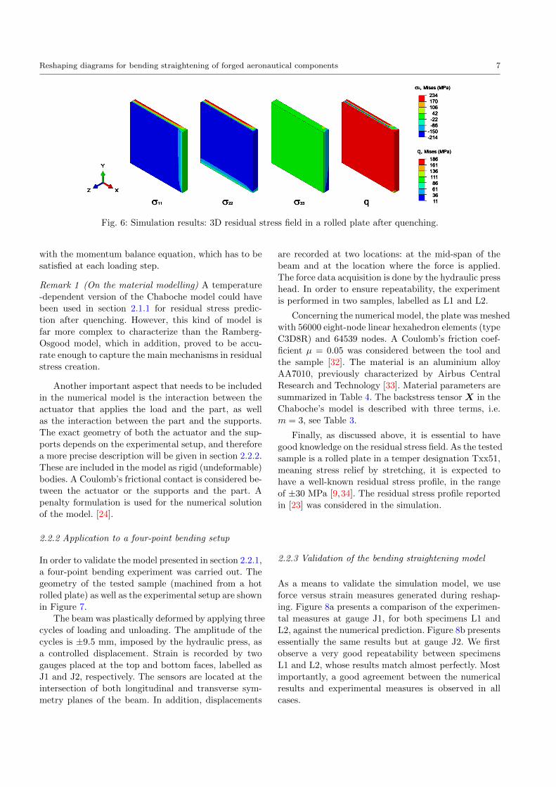
Concerning the numerical model, the plate was meshed
with 64, 000 8-node linear hexahedron elements, with
40 elements in the through-thickness (ST) direction.
The total number of nodes was 68, 921. Abaqus ele-
ment types are DC3D8 for the heat transfer analysis
Reshaping diagrams for bending straightening of forged aeronautical components 5
Table 1: Thermo-plasticity model for quenching simulation.
Thermal step modelling
Energy balance: ρCp∂T∂t
+∇ · q = 0, together with Fourier’s law for the heat flux q = −κ∇T , in Ω × (0, Tfinal].
Initial condition: T = T0 at Ω × 0.Surrounding’s predefined temperature: T∞.
Convective boundary condition: −κ∇T · n = h(T − T∞) on ∂Ω × (0, Tfinal].
ρ, Cp, κ are the material’s mass density, specific heat capacity and thermal conductivity, respectively. h is the heat transfercoefficient. These are taken as a function of the temperature.
n is the outward unit normal to ∂Ω.
Mechanical step modelling
Momentum balance equation: ∇ · σ = 0 in Ω × (0, Tfinal].
Strain decomposition: ε = εe + εp + εth.
Hooke’s law: εe = 12µ
(I− ν
1+νI ⊗ I
): σ with µ = E
2(1+ν), where I denotes the symmetric part of the fourth order
identity tensor and I is the second order identity tensor.
Thermal strain increment: ∆εthij = αδij∆T , where δij is the Kronecker delta.
Yield surface: f (σ) = σ (σ) − σy, where σ (σ) =√
3 J2, J2 = 12s : s and s = σ − 1
3tr (σ) I. On the other hand, σy is the
yield stress.
Ramberg-Osgood isotropic hardening: σy = σy0+ k (εp)n, with the effective plastic strain as εp =
∫ t0
√23εp : εp dt.
Flow rule: εp = γ ∂f∂σ
= γN with N =√
32s‖s‖ .
E and ν are the Young’s modulus and the Poisson’s coefficient, respectively. α is the thermal expansion coefficient and σy0,
k and n are the Ramberg-Osgood model parameters. These are taken as a function of the temperature.
Table 2: Quenching model validation. Quenching process conditions from [19].
ParametersInitial temperature T0 467 CQuenching temperature (cold water) T∞ 20 CQuenching time Tfinal 500 s
and C3D8R for the mechanical step. Figure 4 depicts
the geometry, boundary conditions and mesh of the nu-
merical model.
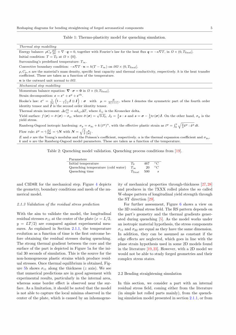
2.1.3 Validation of the residual stress prediction
With the aim to validate the model, the longitudinal
residual stresses σ11 at the center of the plate (x = L/2,
y = LT/2) are compared against experimental mea-
sures. As explained in Section 2.1.1, the temperature
evolution as a function of time is the first outcome be-
fore obtaining the residual stresses during quenching.
The strong thermal gradient between the core and the
surface of the part is depicted in Figure 5a for the ini-
tial 30 seconds of simulation. This is the source for the
non-homogeneous plastic strains which produce resid-
ual stresses. Once thermal equilibrium is obtained, Fig-
ure 5b shows σ11 along the thickness (z axis). We see
that numerical predictions are in good agreement with
experimental results, particularly in the internal area,
whereas some border effect is observed near the sur-
face. As a limitation, it should be noted that the model
is not able to capture the local minima observed in the
center of the plate, which is caused by an inhomogene-
ity of mechanical properties through-thickness [27,28]
and produces in the 7XXX rolled plates the so called
W-shape pattern of longitudinal yield strength through
the ST direction [29].
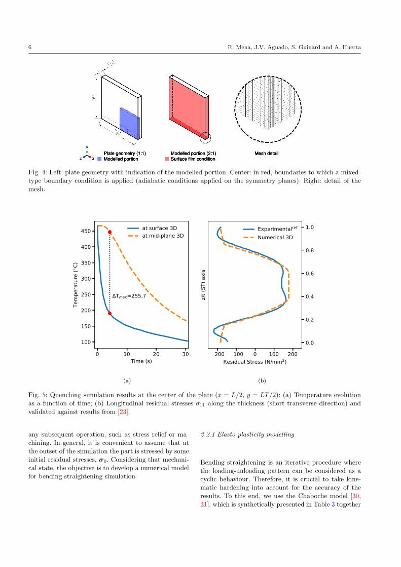
For further assessment, Figure 6 shows a view on
the 3D residual stress field. The RS pattern depends on
the part’s geometry and the thermal gradients gener-
ated during quenching [5]. As the model works under
an isotropic material hypothesis, the stress components
σ11 and σ22 are equal as they have the same dimension.
In addition, they can be assumed as constant if the
edge effects are neglected, which goes in line with the
plane strain hypothesis used in some 2D models found
in the literature [19,23]. However, with a 2D model we
would not be able to study forged geometries and their
complex stress states.
2.2 Bending straightening simulation
In this section, we consider a part with an internal
residual stress field, coming either from the literature
(in simple hot rolled parts mainly), from the quench-
ing simulation model presented in section 2.1.1, or from
6 R. Mena, J.V. Aguado, S. Guinard and A. Huerta
Fig. 4: Left: plate geometry with indication of the modelled portion. Center: in red, boundaries to which a mixed-
type boundary condition is applied (adiabatic conditions applied on the symmetry planes). Right: detail of the
mesh.
0 10 20 30Time (s)
100
150
200
250
300
350
400
450
Tem erature (∘C)
(Tmax=255Δ7
at surface 3Dat mid∘ lane 3D
−200 −100 0 100 200Residual Stress (N/mm2)
0.0
0.2
0.4
0.6
0.8
1.0
z/t (ST) a
xis
ExperimentalrefNumerical 3D
(a)
0 10 20 30Time (s)
100
150
200
250
300
350
400
450
Tem erature (∘C)
(Tmax=255Δ7
at surface 3Dat mid∘ lane 3D
−200 −100 0 100 200Residual Stress (N/mm2)
0.0
0.2
0.4
0.6
0.8
1.0
z/t (ST) a
xis
ExperimentalrefNumerical 3D
(b)
Fig. 5: Quenching simulation results at the center of the plate (x = L/2, y = LT/2): (a) Temperature evolution
as a function of time; (b) Longitudinal residual stresses σ11 along the thickness (short transverse direction) and
validated against results from [23].
any subsequent operation, such as stress relief or ma-
chining. In general, it is convenient to assume that at
the outset of the simulation the part is stressed by some
initial residual stresses, σ0. Considering that mechani-
cal state, the objective is to develop a numerical model
for bending straightening simulation.
2.2.1 Elasto-plasticity modelling
Bending straightening is an iterative procedure where
the loading-unloading pattern can be considered as a
cyclic behaviour. Therefore, it is crucial to take kine-
matic hardening into account for the accuracy of the
results. To this end, we use the Chaboche model [30,
31], which is synthetically presented in Table 3 together
Reshaping diagrams for bending straightening of forged aeronautical components 7
Fig. 6: Simulation results: 3D residual stress field in a rolled plate after quenching.
with the momentum balance equation, which has to be
satisfied at each loading step.
Remark 1 (On the material modelling) A temperature
-dependent version of the Chaboche model could have
been used in section 2.1.1 for residual stress predic-
tion after quenching. However, this kind of model is
far more complex to characterize than the Ramberg-
Osgood model, which in addition, proved to be accu-
rate enough to capture the main mechanisms in residual
stress creation.
Another important aspect that needs to be included
in the numerical model is the interaction between the
actuator that applies the load and the part, as well
as the interaction between the part and the supports.
The exact geometry of both the actuator and the sup-
ports depends on the experimental setup, and therefore
a more precise description will be given in section 2.2.2.
These are included in the model as rigid (undeformable)
bodies. A Coulomb’s frictional contact is considered be-
tween the actuator or the supports and the part. A
penalty formulation is used for the numerical solution
of the model. [24].
2.2.2 Application to a four-point bending setup
In order to validate the model presented in section 2.2.1,
a four-point bending experiment was carried out. The
geometry of the tested sample (machined from a hot
rolled plate) as well as the experimental setup are shown
in Figure 7.
The beam was plastically deformed by applying three
cycles of loading and unloading. The amplitude of the
cycles is ±9.5 mm, imposed by the hydraulic press, as
a controlled displacement. Strain is recorded by two
gauges placed at the top and bottom faces, labelled as
J1 and J2, respectively. The sensors are located at the
intersection of both longitudinal and transverse sym-
metry planes of the beam. In addition, displacements
are recorded at two locations: at the mid-span of the
beam and at the location where the force is applied.
The force data acquisition is done by the hydraulic press
head. In order to ensure repeatability, the experiment
is performed in two samples, labelled as L1 and L2.
Concerning the numerical model, the plate was meshed
with 56000 eight-node linear hexahedron elements (type
C3D8R) and 64539 nodes. A Coulomb’s friction coef-
ficient µ = 0.05 was considered between the tool and
the sample [32]. The material is an aluminium alloy
AA7010, previously characterized by Airbus Central
Research and Technology [33]. Material parameters are
summarized in Table 4. The backstress tensor X in the
Chaboche’s model is described with three terms, i.e.
m = 3, see Table 3.
Finally, as discussed above, it is essential to have
good knowledge on the residual stress field. As the tested
sample is a rolled plate in a temper designation Txx51,
meaning stress relief by stretching, it is expected tohave a well-known residual stress profile, in the range
of ±30 MPa [9,34]. The residual stress profile reported
in [23] was considered in the simulation.
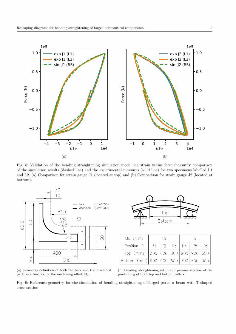
2.2.3 Validation of the bending straightening model
As a means to validate the simulation model, we use
force versus strain measures generated during reshap-
ing. Figure 8a presents a comparison of the experimen-
tal measures at gauge J1, for both specimens L1 and
L2, against the numerical prediction. Figure 8b presents
essentially the same results but at gauge J2. We first
observe a very good repeatability between specimens
L1 and L2, whose results match almost perfectly. Most
importantly, a good agreement between the numerical
results and experimental measures is observed in all
cases.
8 R. Mena, J.V. Aguado, S. Guinard and A. Huerta
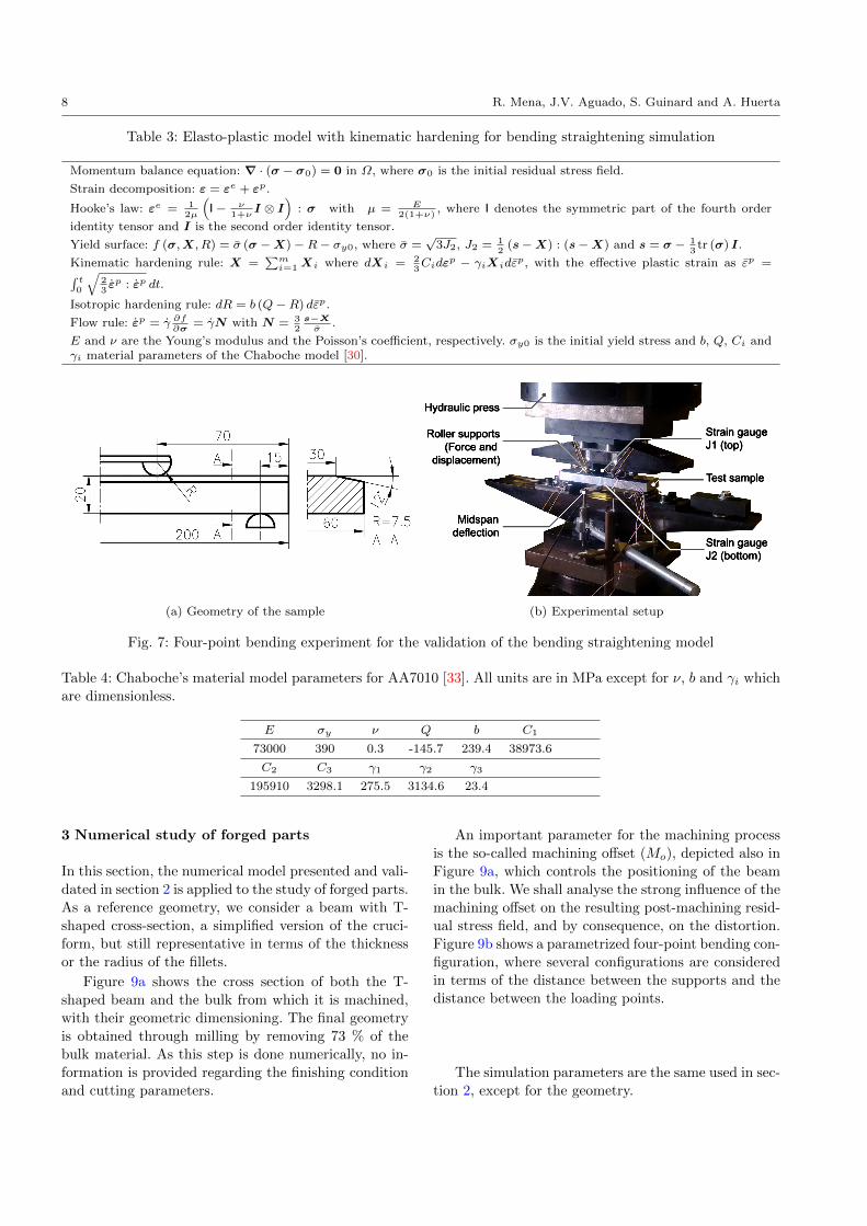
Table 3: Elasto-plastic model with kinematic hardening for bending straightening simulation
Momentum balance equation: ∇ · (σ − σ0) = 0 in Ω, where σ0 is the initial residual stress field.
Strain decomposition: ε = εe + εp.
Hooke’s law: εe = 12µ
(I− ν
1+νI ⊗ I
): σ with µ = E
2(1+ν), where I denotes the symmetric part of the fourth order
identity tensor and I is the second order identity tensor.
Yield surface: f (σ,X, R) = σ (σ −X)−R− σy0, where σ =√
3J2, J2 = 12
(s−X) : (s−X) and s = σ − 13
tr (σ) I.
Kinematic hardening rule: X =∑mi=1Xi where dXi = 2
3Cidεp − γiXidεp, with the effective plastic strain as εp =∫ t
0
√23εp : εp dt.
Isotropic hardening rule: dR = b (Q−R) dεp.
Flow rule: εp = γ ∂f∂σ
= γN with N = 32s−Xσ
.
E and ν are the Young’s modulus and the Poisson’s coefficient, respectively. σy0 is the initial yield stress and b, Q, Ci andγi material parameters of the Chaboche model [30].
(a) Geometry of the sample (b) Experimental setup
Fig. 7: Four-point bending experiment for the validation of the bending straightening model
Table 4: Chaboche’s material model parameters for AA7010 [33]. All units are in MPa except for ν, b and γi which
are dimensionless.
E σy ν Q b C1
73000 390 0.3 -145.7 239.4 38973.6
C2 C3 γ1 γ2 γ3
195910 3298.1 275.5 3134.6 23.4
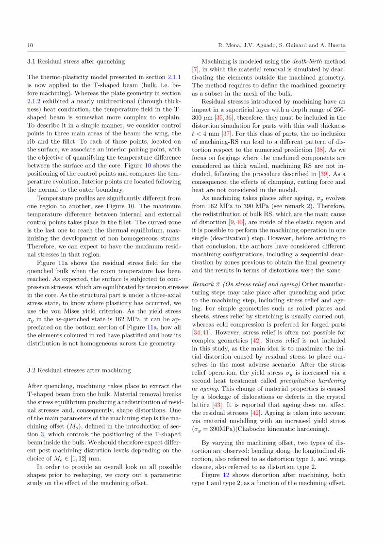
3 Numerical study of forged parts
In this section, the numerical model presented and vali-
dated in section 2 is applied to the study of forged parts.
As a reference geometry, we consider a beam with T-
shaped cross-section, a simplified version of the cruci-
form, but still representative in terms of the thickness
or the radius of the fillets.
Figure 9a shows the cross section of both the T-
shaped beam and the bulk from which it is machined,
with their geometric dimensioning. The final geometry
is obtained through milling by removing 73 % of the
bulk material. As this step is done numerically, no in-
formation is provided regarding the finishing condition
and cutting parameters.
An important parameter for the machining process
is the so-called machining offset (Mo), depicted also in
Figure 9a, which controls the positioning of the beam
in the bulk. We shall analyse the strong influence of the
machining offset on the resulting post-machining resid-
ual stress field, and by consequence, on the distortion.
Figure 9b shows a parametrized four-point bending con-
figuration, where several configurations are considered
in terms of the distance between the supports and the
distance between the loading points.
The simulation parameters are the same used in sec-
tion 2, except for the geometry.
Reshaping diagrams for bending straightening of forged aeronautical components 9
4 3 2 1 0 111 1e4
1.0
0.5
0.0
0.5
1.0
Forc
e (N
)
1e5exp J1 (L1)exp J1 (L2)sim J1 (RS)
1 0 1 2 3 411 1e4
1.0
0.5
0.0
0.5
1.0
Forc
e (N
)
1e5exp J2 (L1)exp J2 (L2)sim J2 (RS)
(a)
4 3 2 1 0 111 1e4
1.0
0.5
0.0
0.5
1.0
Forc
e (N
)
1e5exp J1 (L1)exp J1 (L2)sim J1 (RS)
1 0 1 2 3 411 1e4
1.0
0.5
0.0
0.5
1.0
Forc
e (N
)
1e5exp J2 (L1)exp J2 (L2)sim J2 (RS)
(b)
Fig. 8: Validation of the bending straightening simulation model via strain versus force measures: comparison
of the simulation results (dashed line) and the experimental measures (solid line) for two specimens labelled L1
and L2. (a) Comparison for strain gauge J1 (located at top) and (b) Comparison for strain gauge J2 (located at
bottom).
(a) Geometry definition of both the bulk and the machinedpart, as a function of the machining offset Mo
(b) Bending straightening setup and parametrization of thepositioning of both top and bottom rollers
Fig. 9: Reference geometry for the simulation of bending straightening of forged parts: a beam with T-shaped
cross section
10 R. Mena, J.V. Aguado, S. Guinard and A. Huerta
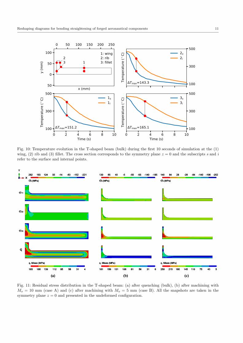
3.1 Residual stress after quenching
The thermo-plasticity model presented in section 2.1.1
is now applied to the T-shaped beam (bulk, i.e. be-
fore machining). Whereas the plate geometry in section
2.1.2 exhibited a nearly unidirectional (through thick-
ness) heat conduction, the temperature field in the T-
shaped beam is somewhat more complex to explain.
To describe it in a simple manner, we consider control
points in three main areas of the beam: the wing, the
rib and the fillet. To each of these points, located on
the surface, we associate an interior pairing point, with
the objective of quantifying the temperature difference
between the surface and the core. Figure 10 shows the
positioning of the control points and compares the tem-
perature evolution. Interior points are located following
the normal to the outer boundary.
Temperature profiles are significantly different from
one region to another, see Figure 10. The maximum
temperature difference between internal and external
control points takes place in the fillet. The curved zone
is the last one to reach the thermal equilibrium, max-
imizing the development of non-homogeneous strains.
Therefore, we can expect to have the maximum resid-
ual stresses in that region.
Figure 11a shows the residual stress field for the
quenched bulk when the room temperature has been
reached. As expected, the surface is subjected to com-
pression stresses, which are equilibrated by tension stresses
in the core. As the structural part is under a three-axial
stress state, to know where plasticity has occurred, we
use the von Mises yield criterion. As the yield stress
σy in the as-quenched state is 162 MPa, it can be ap-
preciated on the bottom section of Figure 11a, how all
the elements coloured in red have plastified and how its
distribution is not homogeneous across the geometry.
3.2 Residual stresses after machining
After quenching, machining takes place to extract the
T-shaped beam from the bulk. Material removal breaks
the stress equilibrium producing a redistribution of resid-
ual stresses and, consequently, shape distortions. One
of the main parameters of the machining step is the ma-
chining offset (Mo), defined in the introduction of sec-
tion 3, which controls the positioning of the T-shaped
beam inside the bulk. We should therefore expect differ-
ent post-machining distortion levels depending on the
choice of Mo ∈ [1, 12] mm.
In order to provide an overall look on all possible
shapes prior to reshaping, we carry out a parametric
study on the effect of the machining offset.
Machining is modeled using the death-birth method
[7], in which the material removal is simulated by deac-
tivating the elements outside the machined geometry.
The method requires to define the machined geometry
as a subset in the mesh of the bulk.
Residual stresses introduced by machining have an
impact in a superficial layer with a depth range of 250-
300 µm [35,36], therefore, they must be included in the
distortion simulation for parts with thin wall thickness
t < 4 mm [37]. For this class of parts, the no inclusion
of machining-RS can lead to a different pattern of dis-
tortion respect to the numerical prediction [38]. As we
focus on forgings where the machined components are
considered as thick walled, machining RS are not in-
cluded, following the procedure described in [39]. As a
consequence, the effects of clamping, cutting force and
heat are not considered in the model.
As machining takes places after ageing, σy evolves
from 162 MPa to 390 MPa (see remark 2). Therefore,
the redistribution of bulk RS, which are the main cause
of distortion [9,40], are inside of the elastic region and
it is possible to perform the machining operation in one
single (deactivation) step. However, before arriving to
that conclusion, the authors have considered different
machining configurations, including a sequential deac-
tivation by zones previous to obtain the final geometry
and the results in terms of distortions were the same.
Remark 2 (On stress relief and ageing) Other manufac-
turing steps may take place after quenching and prior
to the machining step, including stress relief and age-
ing. For simple geometries such as rolled plates and
sheets, stress relief by stretching is usually carried out,
whereas cold compression is preferred for forged parts
[34,41]. However, stress relief is often not possible for
complex geometries [42]. Stress relief is not included
in this study, as the main idea is to maximize the ini-
tial distortion caused by residual stress to place our-
selves in the most adverse scenario. After the stress
relief operation, the yield stress σy is increased via a
second heat treatment called precipitation hardening
or ageing. This change of material properties is caused
by a blockage of dislocations or defects in the crystal
lattice [43]. It is reported that ageing does not affect
the residual stresses [42]. Ageing is taken into account
via material modelling with an increased yield stress
(σy = 390MPa)(Chaboche kinematic hardening).
By varying the machining offset, two types of dis-
tortion are observed: bending along the longitudinal di-
rection, also referred to as distortion type 1, and wings
closure, also referred to as distortion type 2.
Figure 12 shows distortion after machining, both
type 1 and type 2, as a function of the machining offset.
Reshaping diagrams for bending straightening of forged aeronautical components 11
0 50 100 150 200 250
x (mm)−50
0
50
100
(m
m)
1: wing2: rib3: fillet1
23
0 2 4 6 8 10Time (s)
100
300
500
Tempe
rature (
∘C)
ΔTmaxΔ151∘2
1s1i
100
300
500
Tempe
rature (
∘C)
ΔTmaxΔ143∘3
2s2i
0 2 4 6 8 10Time (s)
100
300
500
Tempe
rature (
∘C)
ΔTmaxΔ165∘1
3s3i
Fig. 10: Temperature evolution in the T-shaped beam (bulk) during the first 10 seconds of simulation at the (1)
wing, (2) rib and (3) fillet. The cross section corresponds to the symmetry plane z = 0 and the subscripts s and i
refer to the surface and internal points.
Fig. 11: Residual stress distribution in the T-shaped beam: (a) after quenching (bulk), (b) after machining with
Mo = 10 mm (case A) and (c) after machining with Mo = 5 mm (case B). All the snapshots are taken in the
symmetry plane z = 0 and presented in the undeformed configuration.
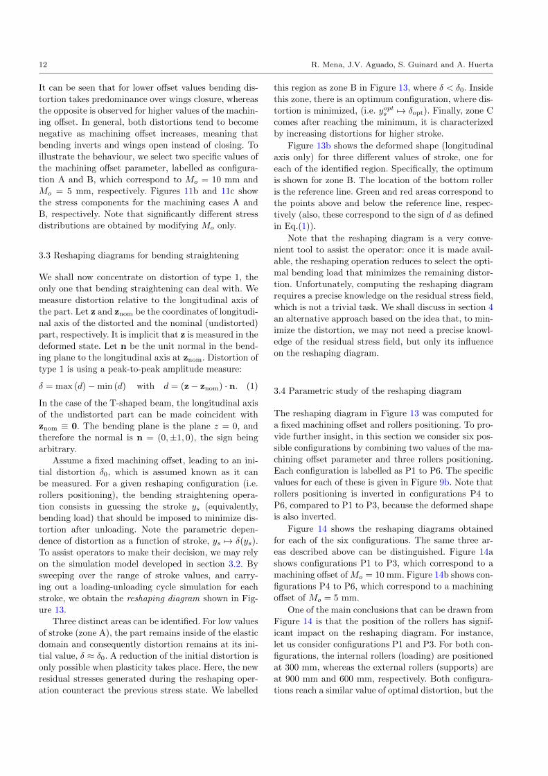
12 R. Mena, J.V. Aguado, S. Guinard and A. Huerta
It can be seen that for lower offset values bending dis-
tortion takes predominance over wings closure, whereas
the opposite is observed for higher values of the machin-
ing offset. In general, both distortions tend to become
negative as machining offset increases, meaning that
bending inverts and wings open instead of closing. To
illustrate the behaviour, we select two specific values of
the machining offset parameter, labelled as configura-
tion A and B, which correspond to Mo = 10 mm and
Mo = 5 mm, respectively. Figures 11b and 11c show
the stress components for the machining cases A and
B, respectively. Note that significantly different stress
distributions are obtained by modifying Mo only.
3.3 Reshaping diagrams for bending straightening
We shall now concentrate on distortion of type 1, the
only one that bending straightening can deal with. We
measure distortion relative to the longitudinal axis of
the part. Let z and znom be the coordinates of longitudi-
nal axis of the distorted and the nominal (undistorted)
part, respectively. It is implicit that z is measured in the
deformed state. Let n be the unit normal in the bend-
ing plane to the longitudinal axis at znom. Distortion of
type 1 is using a peak-to-peak amplitude measure:
δ = max (d)−min (d) with d = (z− znom) · n. (1)
In the case of the T-shaped beam, the longitudinal axis
of the undistorted part can be made coincident with
znom ≡ 0. The bending plane is the plane z = 0, and
therefore the normal is n = (0,±1, 0), the sign being
arbitrary.
Assume a fixed machining offset, leading to an ini-
tial distortion δ0, which is assumed known as it can
be measured. For a given reshaping configuration (i.e.
rollers positioning), the bending straightening opera-
tion consists in guessing the stroke ys (equivalently,
bending load) that should be imposed to minimize dis-
tortion after unloading. Note the parametric depen-
dence of distortion as a function of stroke, ys 7→ δ(ys).
To assist operators to make their decision, we may rely
on the simulation model developed in section 3.2. By
sweeping over the range of stroke values, and carry-
ing out a loading-unloading cycle simulation for each
stroke, we obtain the reshaping diagram shown in Fig-
ure 13.
Three distinct areas can be identified. For low values
of stroke (zone A), the part remains inside of the elastic
domain and consequently distortion remains at its ini-
tial value, δ ≈ δ0. A reduction of the initial distortion is
only possible when plasticity takes place. Here, the new
residual stresses generated during the reshaping oper-
ation counteract the previous stress state. We labelled
this region as zone B in Figure 13, where δ < δ0. Inside
this zone, there is an optimum configuration, where dis-
tortion is minimized, (i.e. yopts 7→ δopt). Finally, zone C
comes after reaching the minimum, it is characterized
by increasing distortions for higher stroke.
Figure 13b shows the deformed shape (longitudinal
axis only) for three different values of stroke, one for
each of the identified region. Specifically, the optimum
is shown for zone B. The location of the bottom roller
is the reference line. Green and red areas correspond to
the points above and below the reference line, respec-
tively (also, these correspond to the sign of d as defined
in Eq.(1)).
Note that the reshaping diagram is a very conve-
nient tool to assist the operator: once it is made avail-
able, the reshaping operation reduces to select the opti-
mal bending load that minimizes the remaining distor-
tion. Unfortunately, computing the reshaping diagram
requires a precise knowledge on the residual stress field,
which is not a trivial task. We shall discuss in section 4
an alternative approach based on the idea that, to min-
imize the distortion, we may not need a precise knowl-
edge of the residual stress field, but only its influence
on the reshaping diagram.
3.4 Parametric study of the reshaping diagram
The reshaping diagram in Figure 13 was computed for
a fixed machining offset and rollers positioning. To pro-
vide further insight, in this section we consider six pos-
sible configurations by combining two values of the ma-
chining offset parameter and three rollers positioning.
Each configuration is labelled as P1 to P6. The specific
values for each of these is given in Figure 9b. Note that
rollers positioning is inverted in configurations P4 to
P6, compared to P1 to P3, because the deformed shape
is also inverted.
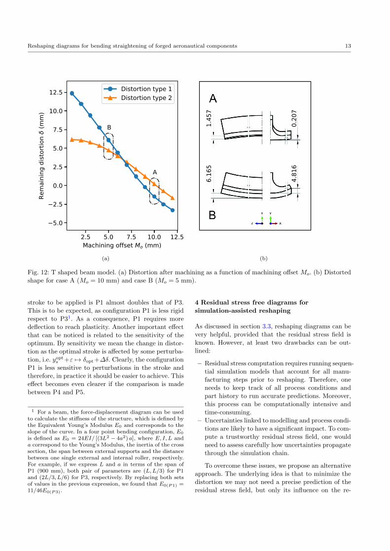
Figure 14 shows the reshaping diagrams obtained
for each of the six configurations. The same three ar-
eas described above can be distinguished. Figure 14a
shows configurations P1 to P3, which correspond to a
machining offset of Mo = 10 mm. Figure 14b shows con-
figurations P4 to P6, which correspond to a machining
offset of Mo = 5 mm.
One of the main conclusions that can be drawn from
Figure 14 is that the position of the rollers has signif-
icant impact on the reshaping diagram. For instance,
let us consider configurations P1 and P3. For both con-
figurations, the internal rollers (loading) are positioned
at 300 mm, whereas the external rollers (supports) are
at 900 mm and 600 mm, respectively. Both configura-
tions reach a similar value of optimal distortion, but the
Reshaping diagrams for bending straightening of forged aeronautical components 13
2.5 5.0 7.5 10.0 12.5Machining offset Mo (mm)
5.0
2.5
0.0
2.5
5.0
7.5
10.0
12.5
Rem
aini
ng d
istor
tion
(mm
)
B
A
Distortion type 1Distortion type 2
1.45
7
0.20
7
6.16
5
4.81
6
(a)
2.5 5.0 7.5 10.0 12.5Machining offset Mo (mm)
5.0
2.5
0.0
2.5
5.0
7.5
10.0
12.5
Rem
aini
ng d
istor
tion
(mm
)
B
A
Distortion type 1Distortion type 2
1.45
7
0.20
7
6.16
5
4.81
6
(b)
Fig. 12: T shaped beam model. (a) Distortion after machining as a function of machining offset Mo. (b) Distorted
shape for case A (Mo = 10 mm) and case B (Mo = 5 mm).
stroke to be applied is P1 almost doubles that of P3.
This is to be expected, as configuration P1 is less rigid
respect to P31. As a consequence, P1 requires more
deflection to reach plasticity. Another important effectthat can be noticed is related to the sensitivity of the
optimum. By sensitivity we mean the change in distor-
tion as the optimal stroke is affected by some perturba-
tion, i.e. yopts +ε 7→ δopt +∆δ. Clearly, the configuration
P1 is less sensitive to perturbations in the stroke and
therefore, in practice it should be easier to achieve. This
effect becomes even clearer if the comparison is made
between P4 and P5.
1 For a beam, the force-displacement diagram can be usedto calculate the stiffness of the structure, which is defined bythe Equivalent Young’s Modulus E0 and corresponds to theslope of the curve. In a four point bending configuration, E0
is defined as E0 = 24EI/ [(3L2 − 4a2) a], where E, I, L anda correspond to the Young’s Modulus, the inertia of the crosssection, the span between external supports and the distancebetween one single external and internal roller, respectively.For example, if we express L and a in terms of the span ofP1 (900 mm), both pair of parameters are (L,L/3) for P1and (2L/3, L/6) for P3, respectively. By replacing both setsof values in the previous expression, we found that E0(P1) =11/46E0(P3).
4 Residual stress free diagrams for
simulation-assisted reshaping
As discussed in section 3.3, reshaping diagrams can be
very helpful, provided that the residual stress field is
known. However, at least two drawbacks can be out-
lined:
– Residual stress computation requires running sequen-
tial simulation models that account for all manu-
facturing steps prior to reshaping. Therefore, one
needs to keep track of all process conditions and
part history to run accurate predictions. Moreover,
this process can be computationally intensive and
time-consuming.
– Uncertainties linked to modelling and process condi-
tions are likely to have a significant impact. To com-
pute a trustworthy residual stress field, one would
need to assess carefully how uncertainties propagate
through the simulation chain.
To overcome these issues, we propose an alternative
approach. The underlying idea is that to minimize the
distortion we may not need a precise prediction of the
residual stress field, but only its influence on the re-

14 R. Mena, J.V. Aguado, S. Guinard and A. Huerta
0.0 yopts
Stroke ys (mm)
0.0
0.2
0.4
0.6
0.8
1.0
1.2
Rem
aini
ng d
istor
tion
(mm
)
ZonesA. No reshaping is performed 0 Optimum configuration = minB. Reshaping takes place < 0 C. Distortion increment > 0°
°
A B C0
1A
0.1
0.0
0.1
Verti
cal d
ispla
cem
ent u
2 (m
m)
B
0 0.5LBeam Length L (mm)
1
0
C
(a)
0.0 yopts
Stroke ys (mm)
0.0
0.2
0.4
0.6
0.8
1.0
1.2
Rem
aini
ng d
istor
tion
(mm
)
ZonesA. No reshaping is performed 0 Optimum configuration = minB. Reshaping takes place < 0 C. Distortion increment > 0°
°
A B C0
1A
0.1
0.0
0.1
Verti
cal d
ispla
cem
ent u
2 (m
m)
B
0 0.5LBeam Length L (mm)
1
0
C
(b)
Fig. 13: Reshaping diagram (scheme). (a) The three characteristic regions of the reshaping diagram: elastic area
of no repair (A), repairing area (B) and inversion area (C). (b) Shape after reshaping for values of the stroke in
each reshaping region.
shaping diagram. Let us consider the parametric study
already presented in section 3. For each of the configu-
rations P1 to P6, we compute the reshaping diagram of
a distorted part but neglecting the residual stress field.
That is, we keep the distorted geometry after machin-
ing but suppress the residual stress field. The results
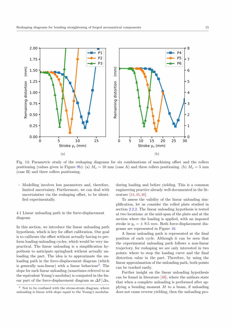
are shown in Figure 15.
From Figure 15 we can conclude that neglecting the
residual stresses results only in a shift of the reshaping
diagram: δ(ys) ≈ δRSF(yRSFs + ∆ys). In other words,
the overall behaviour including a realistic 3D residual
stress field can be retrieved from the residual stress free
diagram, provided that we are able to devise a strategy
to identify the appropriate offset ∆ys.
The reshaping offset can be negative, as in Figure
15a, or positive, as in Figure 15b. To explain this be-
haviour, let us study the P5 configuration. Here, as the
initial distortion has a U shape, bending is applied up-
wards and therefore, tension is induced along the rib.
However, the rib is initially in compression due to the
residual stresses (see σ33 in Figure 11c). As consequence
of this inversion of stresses, more stroke needs to be ap-
plied in order to reach the yield surface, compared to
the residual stress free case. As a general rule, if the
stresses generated during reshaping oppose the initial
residual stresses, the offset will be positive; otherwise,
it will be negative.
The residual stress free approach has many advan-
tages:
– It uses as the main input the initial distortion after
machining, which unlike stresses, can be measured
on a systematic basis.
– The underlying numerical model is rather simple, as
it only needs to account for the bending straighten-
ing step. The computational cost is drastically re-
duced. See Figure 3 for comparison.
Reshaping diagrams for bending straightening of forged aeronautical components 15
0 5 10 15Stroke ys (mm)
0.00
0.25
0.50
0.75
1.00
1.25
1.50
1.75
2.00
Remaining
dist
ortio
n δ (m
m)
P1P2P3
0 5 10 15 20 25 30Stroke ys (mm)
0
1
2
3
4
5
6
7
8
Remaining
dist
ortio
n δ (m
m)
P4P5P6
(a)
0 5 10 15Stroke ys (mm)
0.00
0.25
0.50
0.75
1.00
1.25
1.50
1.75
2.00
Remaining
dist
ortio
n δ (m
m)
P1P2P3
0 5 10 15 20 25 30Stroke ys (mm)
0
1
2
3
4
5
6
7
8
Remaining
dist
ortio
n δ (m
m)
P4P5P6
(b)
Fig. 14: Parametric study of the reshaping diagrams for six combinations of machining offset and the rollers
positioning (values given in Figure 9b): (a) Mo = 10 mm (case A) and three rollers positioning. (b) Mo = 5 mm
(case B) and three rollers positioning.
– Modelling involves less parameters and, therefore,
limited uncertainty. Furthermore, we can deal with
uncertainties via the reshaping offset, to be identi-
fied experimentally.
4.1 Linear unloading path in the force-displacement
diagram
In this section, we introduce the linear unloading path
hypothesis, which is key for offset calibration. Our goal
is to calibrate the offset without actually having to per-
form loading-unloading cycles, which would be very im-
practical. The linear unloading is a simplification hy-
pothesis to anticipate springback without actually un-
loading the part. The idea is to approximate the un-
loading path in the force-displacement diagram (which
is generally non-linear) with a linear behaviour2. The
slope for such linear unloading (sometimes referred to as
the equivalent Young’s modulus) is computed in the lin-
ear part of the force-displacement diagram as ∆F/∆u,
2 Not to be confused with the stress-strain diagram, whereunloading is linear with slope equal to the Young’s modulus.
during loading and before yielding. This is a common
engineering practice already well-documented in the lit-
erature [44,45,46].
To assess the validity of the linear unloading sim-
plification, let us consider the rolled plate studied in
section 2.2.2. The linear unloading hypothesis is tested
at two locations: at the mid-span of the plate and at the
section where the loading is applied, with an imposed
stroke is ys = ± 9.5 mm. Both force-displacement dia-
grams are represented in Figure 16.
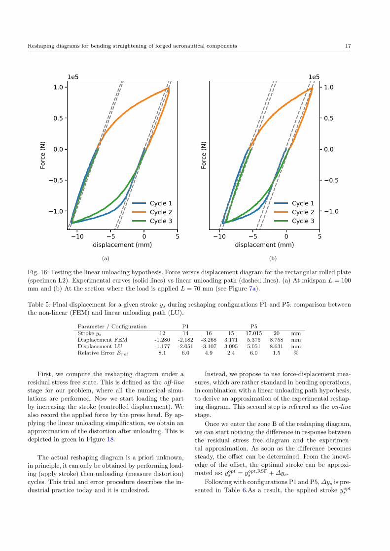
A linear unloading path is represented at the final
position of each cycle. Although it can be seen that
the experimental unloading path follows a non-linear
trajectory, for reshaping we are only interested in two
points: where to stop the loading curve and the final
distortion value in the part. Therefore, by using the
linear approximation of the unloading path, both points
can be tracked easily.
Further insight on the linear unloading hypothesis
can be found in literature [46], where the authors state
that when a complete unloading is performed after ap-
plying a bending moment M to a beam, if unloading
does not cause reverse yielding, then the unloading pro-
16 R. Mena, J.V. Aguado, S. Guinard and A. Huerta
0
1
2
P10
4
8
P4
0
1
2
Remaining
dist
ortio
n δ (m
m)
P20
4
8
Remaining
dist
ortio
n δ (m
m)
P5
0 5 10 15 20Stroke ys (mm)
0
1
2
P3
0 5 10 15 20 25 30Stroke ys (mm)
0
4
8
P6
(a)
0
1
2
P10
4
8
P4
0
1
2
Remaining
dist
ortio
n δ (m
m)
P20
4
8
Remaining
dist
ortio
n δ (m
m)
P5
0 5 10 15 20Stroke ys (mm)
0
1
2
P3
0 5 10 15 20 25 30Stroke ys (mm)
0
4
8
P6
(b)
Fig. 15: Residual stress free reshaping diagrams (dashed line) against true reshaping diagrams that account for
full 3D residual stress field (solid line), for six different reshaping configurations.
cess is equivalent to the elastic effect caused by ap-
plying −M to the beam. Therefore, the key is to not
produce reverse yielding. This phenomenon is present
in metal sheet forming [47], very common in the auto-
motive industry for instance. However, large structural
elements in the aircraft industry can be considered as
thick walled, and the levels of strain under reshaping
are less likely to develop reverse yielding. Therefore,
the unloading path can be approximated to a linear
behaviour.
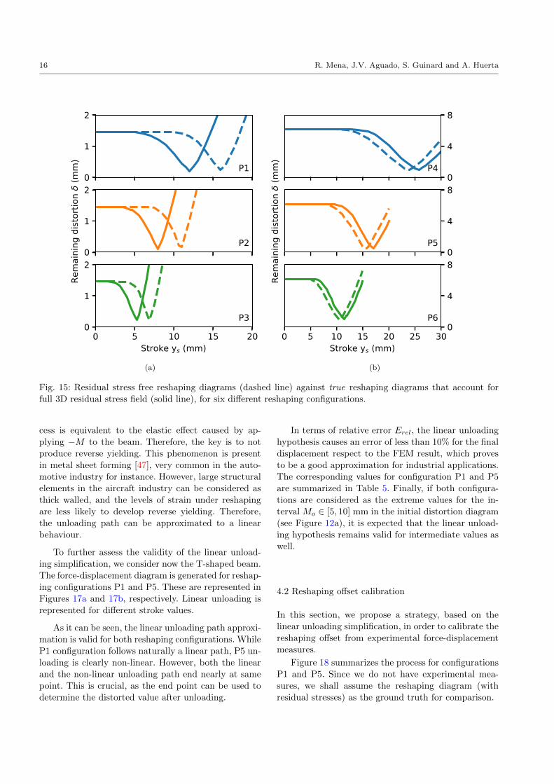
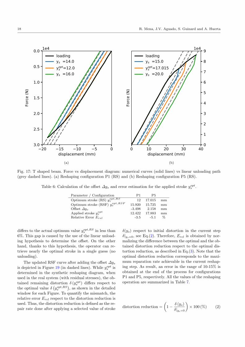
To further assess the validity of the linear unload-
ing simplification, we consider now the T-shaped beam.
The force-displacement diagram is generated for reshap-
ing configurations P1 and P5. These are represented in
Figures 17a and 17b, respectively. Linear unloading is
represented for different stroke values.
As it can be seen, the linear unloading path approxi-
mation is valid for both reshaping configurations. While
P1 configuration follows naturally a linear path, P5 un-
loading is clearly non-linear. However, both the linear
and the non-linear unloading path end nearly at same
point. This is crucial, as the end point can be used to
determine the distorted value after unloading.
In terms of relative error Erel, the linear unloading
hypothesis causes an error of less than 10% for the final
displacement respect to the FEM result, which proves
to be a good approximation for industrial applications.The corresponding values for configuration P1 and P5
are summarized in Table 5. Finally, if both configura-
tions are considered as the extreme values for the in-
terval Mo ∈ [5, 10] mm in the initial distortion diagram
(see Figure 12a), it is expected that the linear unload-
ing hypothesis remains valid for intermediate values as
well.
4.2 Reshaping offset calibration
In this section, we propose a strategy, based on the
linear unloading simplification, in order to calibrate the
reshaping offset from experimental force-displacement
measures.
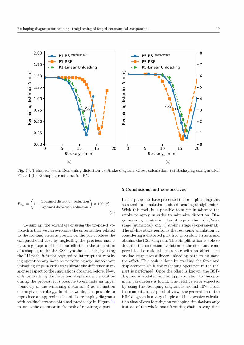
Figure 18 summarizes the process for configurations
P1 and P5. Since we do not have experimental mea-
sures, we shall assume the reshaping diagram (with
residual stresses) as the ground truth for comparison.
Reshaping diagrams for bending straightening of forged aeronautical components 17
−10 −5 0 5displacement (mm)
−1.0
−0.5
0.0
0.5
1.0
Force (N
)
1e5
Cycle 1Cycle 2Cycle 3
−10 −5 0 5displacement (mm)
−1.0
−0.5
0.0
0.5
1.0
Force (N
)
1e5
Cycle 1Cycle 2Cycle 3
(a)
−10 −5 0 5displacement (mm)
−1.0
−0.5
0.0
0.5
1.0
Force (N
)
1e5
Cycle 1Cycle 2Cycle 3
−10 −5 0 5displacement (mm)
−1.0
−0.5
0.0
0.5
1.0
Force (N
)
1e5
Cycle 1Cycle 2Cycle 3
(b)
Fig. 16: Testing the linear unloading hypothesis. Force versus displacement diagram for the rectangular rolled plate
(specimen L2). Experimental curves (solid lines) vs linear unloading path (dashed lines). (a) At midspan L = 100
mm and (b) At the section where the load is applied L = 70 mm (see Figure 7a).
Table 5: Final displacement for a given stroke ys during reshaping configurations P1 and P5: comparison between
the non-linear (FEM) and linear unloading path (LU).
Parameter / Configuration P1 P5Stroke ys 12 14 16 15 17.015 20 mmDisplacement FEM -1.280 -2.182 -3.268 3.171 5.376 8.758 mmDisplacement LU -1.177 -2.051 -3.107 3.095 5.051 8.631 mmRelative Error Erel 8.1 6.0 4.9 2.4 6.0 1.5 %
First, we compute the reshaping diagram under a
residual stress free state. This is defined as the off-line
stage for our problem, where all the numerical simu-
lations are performed. Now we start loading the part
by increasing the stroke (controlled displacement). We
also record the applied force by the press head. By ap-
plying the linear unloading simplification, we obtain an
approximation of the distortion after unloading. This is
depicted in green in Figure 18.
The actual reshaping diagram is a priori unknown,
in principle, it can only be obtained by performing load-
ing (apply stroke) then unloading (measure distortion)
cycles. This trial and error procedure describes the in-
dustrial practice today and it is undesired.
Instead, we propose to use force-displacement mea-
sures, which are rather standard in bending operations,
in combination with a linear unloading path hypothesis,
to derive an approximation of the experimental reshap-
ing diagram. This second step is referred as the on-line
stage.
Once we enter the zone B of the reshaping diagram,
we can start noticing the difference in response between
the residual stress free diagram and the experimen-
tal approximation. As soon as the difference becomes
steady, the offset can be determined. From the knowl-
edge of the offset, the optimal stroke can be approxi-
mated as: yopts = yopt,RSF
s +∆ys.
Following with configurations P1 and P5,∆ys is pre-
sented in Table 6.As a result, the applied stroke yopts
18 R. Mena, J.V. Aguado, S. Guinard and A. Huerta
−20 −15 −10 −5 0displacement (mm)
3.0
2.5
2.0
1.5
1.0
0.5
0.0
Force (N)
1e4loadingys =14.0yopts =12.0ys =16.0
0 10 20 30 40displacement (mm)
0
1
2
3
4
5
6
7
8
9
Force (N)
1e4loadingys =15.0yopts =17.015ys =20.0
(a)
−20 −15 −10 −5 0displacement (mm)
3.0
2.5
2.0
1.5
1.0
0.5
0.0
Force (N)
1e4loadingys =14.0yopts =12.0ys =16.0
0 10 20 30 40displacement (mm)
0
1
2
3
4
5
6
7
8
9
Force (N)
1e4loadingys =15.0yopts =17.015ys =20.0
(b)
Fig. 17: T shaped beam. Force vs displacement diagram: numerical curves (solid lines) vs linear unloading path
(grey dashed lines). (a) Reshaping configuration P1 (RS) and (b) Reshaping configuration P5 (RS).
Table 6: Calculation of the offset ∆ys and error estimation for the applied stroke yopts .
Parameter / Configuration P1 P5
Optimum stroke (RS) yopt,RSs 12 17.015 mm
Optimum stroke (RSF) yopt,RSFs 15.920 15.725 mmOffset ∆ys -3.498 2.158 mm
Applied stroke yopts 12.422 17.883 mmRelative Error Erel -3.5 -5.1 %
differs to the actual optimum value yopt,RSs in less than
6%. This gap is caused by the use of the linear unload-
ing hypothesis to determine the offset. On the other
hand, thanks to this hypothesis, the operator can re-
trieve nearly the optimal stroke in a single guess (no
unloading).
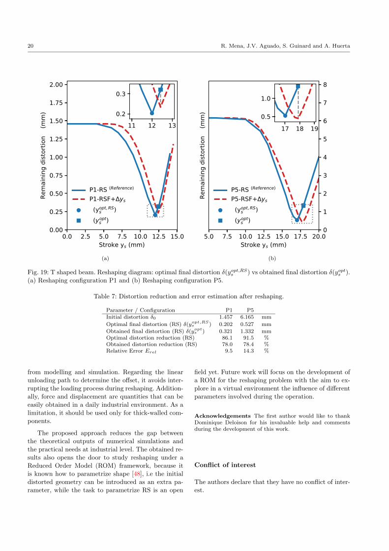
The updated RSF curve after adding the offset ∆ysis depicted in Figure 19 (in dashed lines). While yopts is
determined in the synthetic reshaping diagram, when
used in the real system (with residual stresses), the ob-
tained remaining distortion δ (yopts ) differs respect to
the optimal value δ(yopt,RSs
), as shown in the detailed
window for each Figure. To quantify the mismatch, the
relative error Erel respect to the distortion reduction is
used. Thus, the distortion reduction is defined as the re-
pair rate done after applying a selected value of stroke
δ(ys) respect to initial distortion in the current step
δ|ys=0, see Eq.(2). Therefore, Erel is obtained by nor-
malizing the difference between the optimal and the ob-
tained distortion reduction respect to the optimal dis-
tortion reduction, as described in Eq.(3). Note that the
optimal distortion reduction corresponds to the maxi-
mum reparation rate achievable in the current reshap-
ing step. As result, an error in the range of 10-15% is
obtained at the end of the process for configurations
P1 and P5, respectively. All the values of the reshaping
operation are summarized in Table 7.
distortion reduction =
(1− δ (ys)
δ|ys=0
)× 100 (%) (2)
Reshaping diagrams for bending straightening of forged aeronautical components 19
0 5 10 15 20Stroke ys (mm)
0.00
0.25
0.50
0.75
1.00
1.25
1.50
1.75
2.00
Rem
aini
ng d
istor
tion
(mm
)
ys
P1-RS (Reference)
P1-RSFP1-Linear Unloading
0 5 10 15 20Stroke ys (mm)
0
1
2
3
4
5
6
7
8
Rem
aini
ng d
istor
tion
(mm
)
ys
P5-RS (Reference)
P5-RSFP5-Linear Unloading
(a)
0 5 10 15 20Stroke ys (mm)
0.00
0.25
0.50
0.75
1.00
1.25
1.50
1.75
2.00
Rem
aini
ng d
istor
tion
(mm
)
ys
P1-RS (Reference)
P1-RSFP1-Linear Unloading
0 5 10 15 20Stroke ys (mm)
0
1
2
3
4
5
6
7
8
Rem
aini
ng d
istor
tion
(mm
)
ys
P5-RS (Reference)
P5-RSFP5-Linear Unloading
(b)
Fig. 18: T shaped beam. Remaining distortion vs Stroke diagram: Offset calculation. (a) Reshaping configuration
P1 and (b) Reshaping configuration P5.
Erel =
(1− Obtained distortion reduction
Optimal distortion reduction
)× 100 (%)
(3)
To sum up, the advantage of using the proposed ap-
proach is that we can overcome the uncertainties related
to the residual stresses present on the part, reduce the
computational cost by neglecting the previous manu-
facturing steps and focus our efforts on the simulation
of reshaping under the RSF hypothesis. Then, by using
the LU path, it is not required to interrupt the repair-
ing operation any more by performing any unnecessary
unloading steps in order to calibrate the difference in re-
sponse respect to the simulations obtained before. Now,
only by tracking the force and displacement evolution
during the process, it is possible to estimate an upper
boundary of the remaining distortion δ as a function
of the given stroke ys. In other words, it is possible to
reproduce an approximation of the reshaping diagrams
with residual stresses obtained previously in Figure 14
to assist the operator in the task of repairing a part.
5 Conclusions and perspectives
In this paper, we have presented the reshaping diagrams
as a tool for simulation assisted bending straightening.
With this tool, it is possible to select in advance the
stroke to apply in order to minimize distortion. Dia-
grams are generated in a two step procedure: i) off-line
stage (numerical) and ii) on-line stage (experimental).
The off-line stage performs the reshaping simulation by
considering a distorted part free of residual stresses and
obtains the RSF-diagram. This simplification is able to
describe the distortion evolution of the structure com-
pared to the residual stress case with an offset. The
on-line stage uses a linear unloading path to estimate
the offset. This task is done by tracking the force and
displacement while the reshaping operation in the real
part is performed. Once the offset is known, the RSF-
diagram is updated and an approximation to the opti-
mum parameters is found. The relative error expected
by using the reshaping diagram is around 10%. From
the computational point of view, the generation of the
RSF-diagram is a very simple and inexpensive calcula-
tion that allows focusing on reshaping simulations only
instead of the whole manufacturing chain, saving time
20 R. Mena, J.V. Aguado, S. Guinard and A. Huerta
0.0 2.5 5.0 7.5 10.0 12.5 15.0Stroke ys (mm)
0.00
0.25
0.50
0.75
1.00
1.25
1.50
1.75
2.00
Rem
aini
ng d
is or
ion δ
(mm
)
P1-RS (Reference)P1-RSF+Δysδ(yoptΔRS
s )δ(yopt
s )
5.0 7.5 10.0 12.5 15.0 17.5 20.0S roke ys (mm)
0
1
2
3
4
5
6
7
8
Rem
aini
ng d
is or
ion δ
(mm
)P5-RS (Reference)P5-RSF+Δysδ(yoptΔRS
s )δ(yopt
s )
11 12 130.2
0.3
17 18 190.5
1.0
(a)
0.0 2.5 5.0 7.5 10.0 12.5 15.0Stroke ys (mm)
0.00
0.25
0.50
0.75
1.00
1.25
1.50
1.75
2.00
Rem
aini
ng d
is or
ion δ
(mm
)
P1-RS (Reference)P1-RSF+Δysδ(yoptΔRS
s )δ(yopt
s )
5.0 7.5 10.0 12.5 15.0 17.5 20.0S roke ys (mm)
0
1
2
3
4
5
6
7
8
Rem
aini
ng d
is or
ion δ
(mm
)P5-RS (Reference)P5-RSF+Δysδ(yoptΔRS
s )δ(yopt
s )
11 12 130.2
0.3
17 18 190.5
1.0
(b)
Fig. 19: T shaped beam. Reshaping diagram: optimal final distortion δ(yopt,RSs ) vs obtained final distortion δ(yopts ).
(a) Reshaping configuration P1 and (b) Reshaping configuration P5.
Table 7: Distortion reduction and error estimation after reshaping.
Parameter / Configuration P1 P5Initial distortion δ0 1.457 6.165 mm
Optimal final distortion (RS) δ(yopt,RSs ) 0.202 0.527 mm
Obtained final distortion (RS) δ(yopts ) 0.321 1.332 mmOptimal distortion reduction (RS) 86.1 91.5 %Obtained distortion reduction (RS) 78.0 78.4 %Relative Error Erel 9.5 14.3 %
from modelling and simulation. Regarding the linear
unloading path to determine the offset, it avoids inter-
rupting the loading process during reshaping. Addition-
ally, force and displacement are quantities that can be
easily obtained in a daily industrial environment. As a
limitation, it should be used only for thick-walled com-
ponents.
The proposed approach reduces the gap between
the theoretical outputs of numerical simulations and
the practical needs at industrial level. The obtained re-
sults also opens the door to study reshaping under a
Reduced Order Model (ROM) framework, because it
is known how to parametrize shape [48], i.e the initial
distorted geometry can be introduced as an extra pa-
rameter, while the task to parametrize RS is an open
field yet. Future work will focus on the development of
a ROM for the reshaping problem with the aim to ex-
plore in a virtual environment the influence of different
parameters involved during the operation.
Acknowledgements The first author would like to thankDominique Deloison for his invaluable help and commentsduring the development of this work.
Conflict of interest
The authors declare that they have no conflict of inter-
est.
Reshaping diagrams for bending straightening of forged aeronautical components 21
References
1. Serope Kalpakjian and Schmid Steven. ManufacturingProcesses for Engineering Materials. 7th edition, 2014.
2. S. Narahari Prasad, P. Rambabu, and N. Eswara Prasad.Processing of Aerospace Metals and Alloys: Part 2 - Sec-ondary Processing. In N. Prasad, Eswara, and R.J.H.Wanhill, editors, Aerospace Materials and Material Tech-nologies, volume 2, pages 199–228. Springer Singapore,2017.
3. Guilles Marin. Calcul et optimisation des structuresmecaniques. PhD thesis, Universite TechnologiqueCompiegne, 2000.
4. Tiffany Dux. Forging of Aluminum Alloys. In Kevin An-derson, John Weritz, and J. Gilbert Kaufman, editors,Aluminum Science and Technology, volume 14, pages315–335. ASM International, 2018.
5. J.S. Robinson, S. Hossain, C.E. Truman, A.M. Parad-owska, D.J. Hughes, R.C. Wimpory, and M.E. Fox.Residual stress in 7449 aluminium alloy forgings. Mate-rials Science and Engineering: A, 527(10-11):2603–2612,2010.
6. J. S. Robinson, D. A. Tanner, C. E. Truman, and R. C.Wimpory. Measurement and Prediction of MachiningInduced Redistribution of Residual Stress in the Alu-minium Alloy 7449. Experimental Mechanics, 51(6):981–993, 2011.
7. Kong Ma, Robert Goetz, and Shesh K. Srivatsa. Mod-eling of Residual Stress and Machining Distortion inAerospace Components. In D.U. Furrer and S.L. Semi-atin, editors, Metals Process Simulation, pages 386–407.ASM International, 2010.
8. D M Bowden, B J Sova, A L Beisiegel, and J E Halley.Machined Component Quality Improvements ThroughManufacturing Process Simulation. SAE Technical Paper2001-01-2607, 2001.
9. W. Sim. Challenges of residual stress and part distortionin the civil airframe industry. In 2nd International Con-ference on Distortion Engineering, pages 87–94, 2008.
10. Airbus. A380 - a new century, a new aircraft. AircraftEngineering and Aerospace Technology, 76(4), 2004.
11. Manfred Mitze. Straightening heat-treated components.Journal of Heat Treatment and Materials, 65:110–117,2010.
12. Arne Ellermann and Berthold Scholtes. Residual stressstates as a result of bending and straightening processesof steels in different heat treatment conditions. Interna-tional Journal of Materials Research, 103(1):57–65, 2012.
13. Marvin R. Scott. Torsion straightener, U.S. Patent3451245A, Jun. 1969.
14. Yong Lin Pi and N. S. Trahair. Inelastic Torsion of SteelI-Beams. Journal of Structural Engineering, 121(4):609–620, 1995.
15. R. L. Murthy and B. Kotiveerachari. Burnishing ofmetallic surfaces - a review. Precision Engineering,3:172–179, 1981.
16. H. E. Coules, G. C.M. Horne, S. Kabra, P. Colegrove, andD. J. Smith. Three-dimensional mapping of the residualstress field in a locally-rolled aluminium alloy specimen.Journal of Manufacturing Processes, 26:240–251, 2017.
17. J. Schijve. Residual Stress. In Fatigue of Structures andMaterials, pages 89–104. 2009.
18. Fei Yin, Milan Rakita, Shan Hu, and Qingyou Han.Overview of ultrasonic shot peening. Surface Engineer-ing, 33(9):651–666, 2017.
19. P. Jeanmart and J. Bouvaist. Finite element calculationand measurement of thermal stresses in quenched plates
of high-strength 7075 aluminium alloy. Materials Scienceand Technology, 1(October):765–769, 1985.
20. Xavier Cerutti. Numerical modelling and mechanicalanalysis of the machining of large aeronautical parts:Machining quality improvement. PhD thesis, Ecole Na-tionale Superieure des Mines de Paris, 2014.
21. Zheng Zhang, Liang Li, Yinfei Yang, Ning He, and WeiZhao. Machining distortion minimization for the manu-facturing of aeronautical structure. International Journalof Advanced Manufacturing Technology, 73(9-12):1765–1773, 2014.
22. Zheng Zhang, Yinfei Yang, Liang Li, Bo Chen, and HuiTian. Assessment of residual stress of 7050-T7452 alu-minum alloy forging using the contour method. MaterialsScience and Engineering A, 644:61–68, 2015.
23. Michael Prime, Michael B; Hill. Residual Stress, StressRelief, and Inhomogeneity in Aluminum Plate. ScriptaMaterialia, 46:77–82, 2002.
24. Michael Smith. ABAQUS/Standard User’s Manual, Ver-sion 6.9. Simulia, 2009.
25. Andrzej S luzalec. Introduction to Nonlinear Thermome-chanics. Springer-Verlag London, 1992.
26. W. Ramberg and W. R Osgood. Description of stress-strain curves by three parameters, 1943.
27. Henk F. De Jong. Thickness direction inhomogeneityof mechanical properties and fracture toughness as ob-served in aluminium 7075-t651 plate material. Engineer-ing Fracture Mechanics, 13(1):175 – 192, 1980.
28. Truszkowski W., Krol J., and Major B. Inhomogeneity ofrolling texture in fcc metals. Metallurgical TransactionsA, 11:749–758, 1980.
29. D.J. Chakrabarti, Hasso Weiland, B.A. Cheney, andJames T. Staley. Through thickness property variationsin 7050 plate. In Aluminium Alloys - ICAA5, volume217 of Materials Science Forum, pages 1085–1090. TransTech Publications Ltd, 5 1996.
30. Jean-Louis Chaboche. Time-independent constitutivetheories for cyclic plasticity. International Journal ofPlasticity, 2(2):149–188, 1986.
31. Laurence Portier, Sylvain Calloch, Didier Marquis, andPhilippe Geyer. Ratchetting under tension-torsion load-ings: Experiments and modelling. International journalof plasticity, 2000.
32. Muammer Koc, John Culp, and Taylan Altan. Predic-tion of residual stresses in quenched aluminum blocks andtheir reduction through cold working processes. Jour-nal of Materials Processing Technology, 174(1-3):342–354, 2006.
33. Dominique Deloison and Fabrice Congourdeau. AirbusA380 Fatigue test plan. Technical report, Airbus CentralResearch and Technology, Suresnes, 2016.
34. J. S. Robinson, D. A. Tanner, and C. E. Truman. 50thanniversary article: The origin and management of resid-ual stress in heat-treatable aluminium alloys. Strain,50(3):185–207, 2014.
35. S. Dreier, J. Bruning, and B. Denkena. Simulation basedreduction of residual stress related part distortion. Ma-terialwissenschaft und Werkstofftechnik, 47(8):710–717,2016.
36. I. Lazoglu, D. Ulutan, B.E. Alaca, S. Engin, and B. Kaf-tanoglu. An enhanced analytical model for residual stressprediction in machining. CIRP Annals, 57(1):81–84,2008.
37. W. Sim. Residual Stress Engineering in Manufacture ofAerospace Structural Parts. 3rd International Confer-ence on Distorsions Engineering, pages 187–194, 2011.
22 R. Mena, J.V. Aguado, S. Guinard and A. Huerta
38. A. Madariaga, I. Perez, P. J. Arrazola, R. Sanchez, J. J.Ruiz, and F. J. Rubio. Reduction of distortions in largealuminium parts by controlling machining-induced resid-ual stresses. The International Journal of AdvancedManufacturing Technology, 97:967–978, 2018.
39. Liangbao Liu, Jianfei Sun, Wuyi Chen, and Pengfei Sun.Study on the machining distortion of aluminum alloyparts induced by forging residual stresses. Proceedings ofthe Institution of Mechanical Engineers, Part B: Journalof Engineering Manufacture, 231(4):618–627, 2017.
40. Jian Guang Li and Shu Qi Wang. Distortion causedby residual stresses in machining aeronautical aluminumalloy parts: recent advances. International Journal ofAdvanced Manufacturing Technology, 89(1-4):997–1012,2017.
41. J.S. Robinson, R.C. Wimpory, D.A. Tanner, B. Mooney,C.E Truman, and T. Panzner. Cold Compression of 7075and Factors Influencing Stress Relief. Materials Perfor-mance and Characterization, 7(4):898–911, 2018.
42. J. S. Robinson, D. A. Tanner, S. Van Petegem, andA. Evans. Influence of quenching and aging on resid-ual stress in Al-Zn-Mg-Cu alloy 7449. Materials Scienceand Technology, 28(4):420–430, 2012.
43. H. R. Shercliff and M. F. Ashby. A process model forage hardening of aluminium alloys-I. The model. ActaMetallurgica Et Materialia, 38(10):1789–1802, 1990.
44. Takaai Katoh, Eizo Urata, Minoru Nakanishi, and KazuoYamazaki. Control for Straightening Process of SeamlessPipe. JSME, 34(3):427–432, 1991.
45. G. Forrest. Internal or Residual Stresses in Wrought Alu-minium Alloys and their Structural Significance. Journalof the Royal Aeronautical Society, pages 261–276, 1954.
46. T. X. Yu and Liang chi Zhang. Plastic Bending: Theoryand Applications. World Scientific, 1996.
47. Dorel Banabic. Sheet Metal Forming Processes: Consti-tutive Modelling and Numerical Simulation. Springer,2010.
48. Nathan Lauzeral, Domenico Borzacchiello, Michael Ku-gler, Daniel George, Yves Remond, Alexandre Hostettler,and Francisco Chinesta. Shape parametrization of bio-mechanical finite element models based on medical im-ages. Computer Methods in Biomechanics and Biomed-ical Engineering: Imaging & Visualization, 7(5-6):480–489, 2019.