Embed Size (px)
Citation preview
Réseaux génétiques de Thomas
multivalués
et logique temporelle
Gilles Bernot
University of Nice sophia antipolis, I3S laboratory, France
Acknowledgments:
Observability Group of the Epigenomics Project
1
Menu
1. Modelling biological regulatory networks
2. Discrete framework for biological regulatory networks
3. Temporal logic and Model Checking for biology
4. Computer aided elaboration of formal models
5. Pedagogical example: Pseudomonas aeruginosa
6. Some current research topics
2
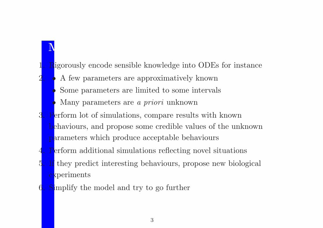
Mathematical Models and Simulation
1. Rigorously encode sensible knowledge into ODEs for instance
2. • A few parameters are approximatively known
• Some parameters are limited to some intervals
• Many parameters are a priori unknown
3. Perform lot of simulations, compare results with known
behaviours, and propose some credible values of the unknown
parameters which produce acceptable behaviours
4. Perform additional simulations reflecting novel situations
5. If they predict interesting behaviours, propose new biological
experiments
6. Simplify the model and try to go further
3
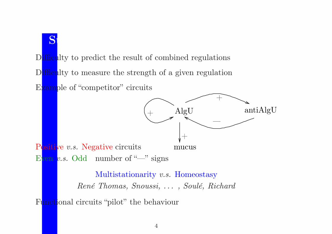
Static Graph v.s. Dynamic Behaviour
Difficulty to predict the result of combined regulations
Difficulty to measure the strength of a given regulation
Example of “competitor” circuits
Positive v.s. Negative circuits
—
+
+
AlgU antiAlgU
mucus
+
Even v.s. Odd number of “—” signs
Multistationarity v.s. Homeostasy
René Thomas, Snoussi, . . . , Soulé, Richard
Functional circuits “pilot” the behaviour
4
Mathematical Models and Validation
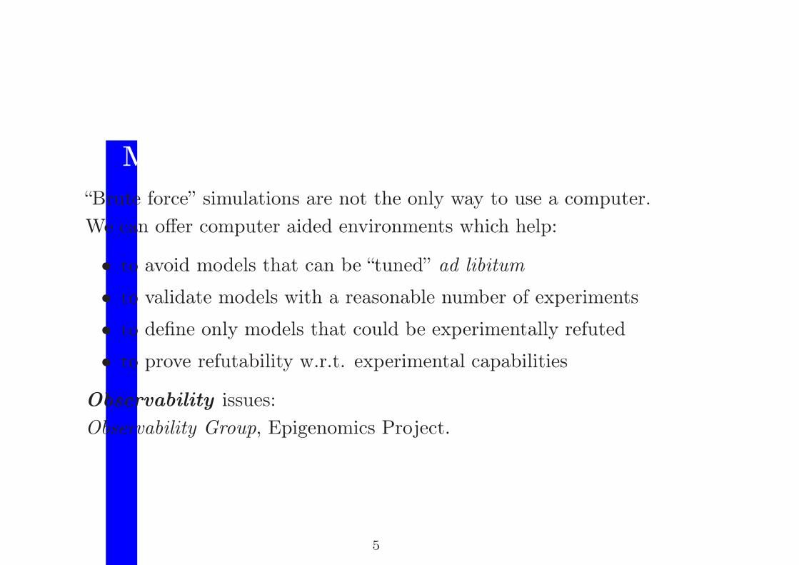
“Brute force” simulations are not the only way to use a computer.
We can offer computer aided environments which help:
• to avoid models that can be “tuned” ad libitum
• to validate models with a reasonable number of experiments
• to define only models that could be experimentally refuted
• to prove refutability w.r.t. experimental capabilities
Observability issues:
Observability Group, Epigenomics Project.
5
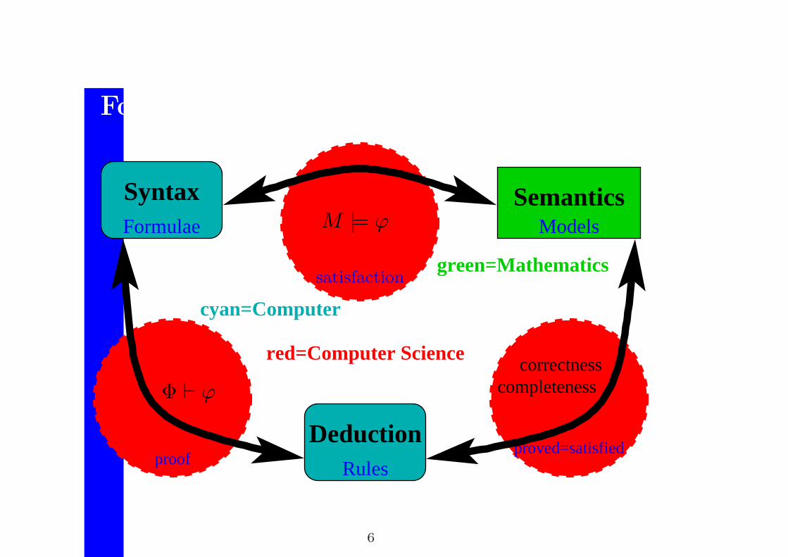
Formal Logic: syntax/semantics/deduction
cyan=Computer
green=Mathematics
correctness
Rulesproof
SemanticsModels
Syntax
Deductionproved=satisfied
completeness
Formulae
red=Computer Science
M |= ϕ
Φ ⊢ ϕ
satisfaction
6

Menu
1. Modelling biological regulatory networks
2. Discrete framework for biological regulatory networks
3. Temporal logic and Model Checking for biology
4. Computer aided elaboration of formal models
5. Pedagogical example: Pseudomonas aeruginosa
6. Some current research topics
7
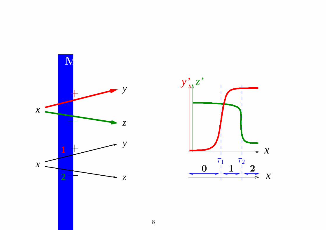
Multivalued Regulatory Graphs
x
x
y
z
y
z2
1
—
—
+
+ x
z’
x
y’
τ20 1 2
τ1
8
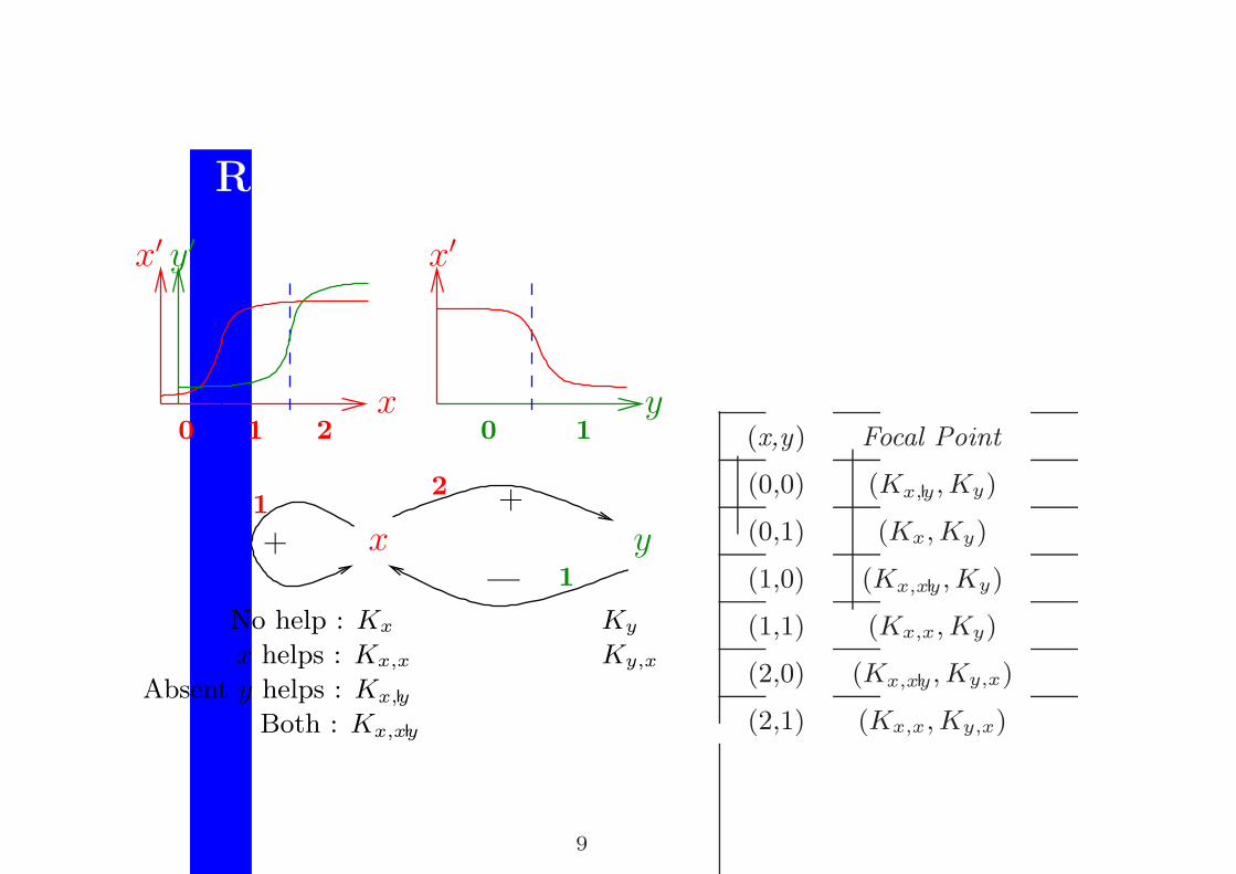
Regulatory Networks (R. Thomas)
y0 1
x′
x1 20
x′ y′
Ky
12
—
x y
+
1
No help : Kx
x helps : Kx,x Ky,x
Absent y helps : Kx,y
Both : Kx,xy
+
(x,y) Focal Point
(0,0) (Kx,y,Ky)
(0,1) (Kx, Ky)
(1,0) (Kx,xy,Ky)
(1,1) (Kx,x, Ky)
(2,0) (Kx,xy, Ky,x)
(2,1) (Kx,x, Ky,x)
9
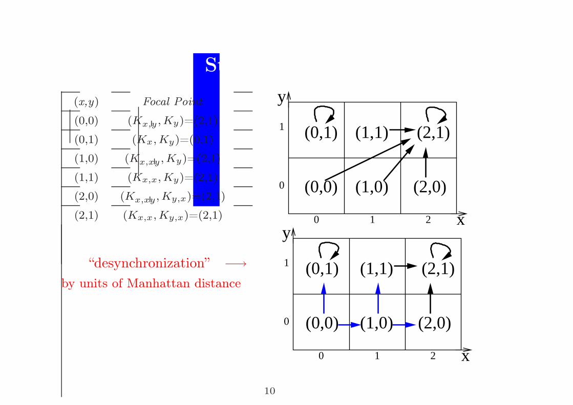
State Graphs
(x,y) Focal Point
(0,0) (Kx,y , Ky)=(2,1)
(0,1) (Kx, Ky)=(0,1)
(1,0) (Kx,xy , Ky)=(2,1)
(1,1) (Kx,x, Ky)=(2,1)
(2,0) (Kx,xy , Ky,x)=(2,1)
(2,1) (Kx,x, Ky,x)=(2,1)
y
x
0
1 (1,1)(0,1)
(0,0) (1,0) (2,0)
(2,1)
0 1 2
“desynchronization” −→
by units of Manhattan distance
y
x
0
1 (1,1)
(1,0) (2,0)
(2,1)
(0,0)
(0,1)
0 1 2
10
Menu
1. Modelling biological regulatory networks
2. Discrete framework for biological regulatory networks
3. Temporal logic and Model Checking for biology
4. Computer Aided elaboration Of Formal models
5. Pedagogical example: Pseudomonas aeruginosa
6. Some current research topics
11
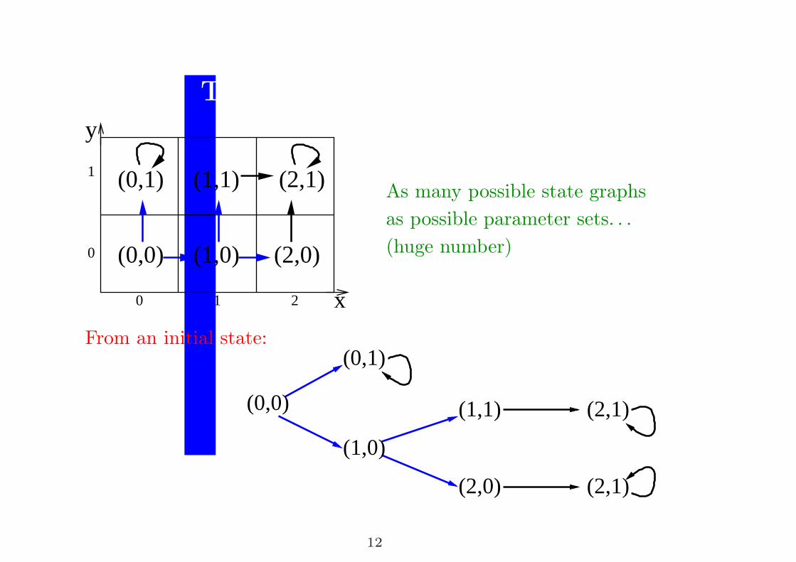
Time has a tree structure
y
x
0
1 (1,1)
(1,0) (2,0)
(2,1)
(0,0)
(0,1)
0 1 2
As many possible state graphs
as possible parameter sets. . .
(huge number)
From an initial state:
(2,1)
(2,1)(1,1)
(2,0)
(1,0)
(0,1)
(0,0)
12
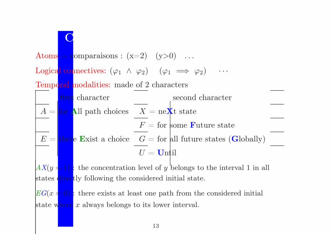
CTL = Computation Tree Logic
Atoms = comparaisons : (x=2) (y>0) . . .
Logical connectives: (ϕ1 ∧ ϕ2) (ϕ1 =⇒ ϕ2) · · ·
Temporal modalities: made of 2 characters
first character second character
A = for All path choices X = neXt state
F = for some Future state
E = there Exist a choice G = for all future states (Globally)
U = Until
AX(y = 1) : the concentration level of y belongs to the interval 1 in all
states directly following the considered initial state.
EG(x = 0) : there exists at least one path from the considered initial
state where x always belongs to its lower interval.
13
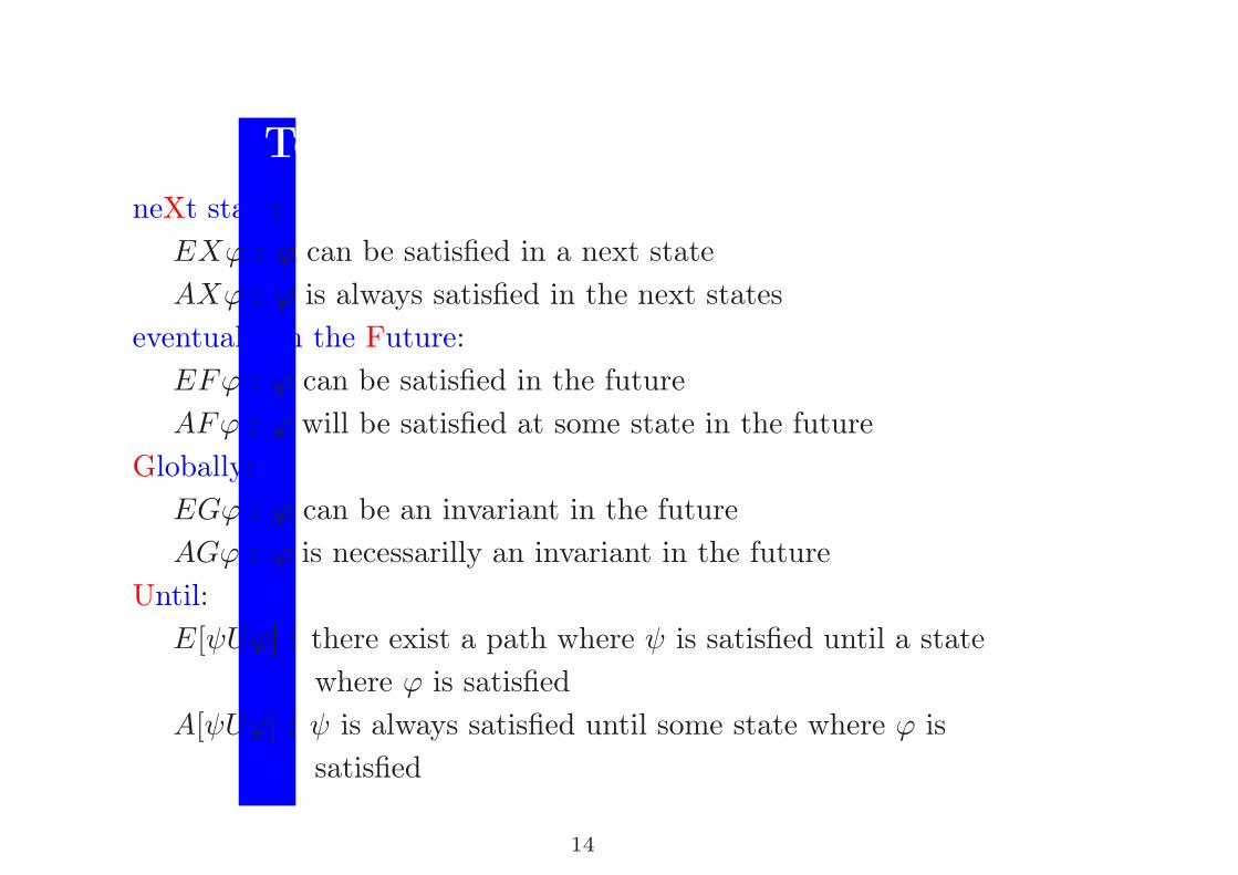
Temporal Connectives of CTL
neXt state:
EXϕ : ϕ can be satisfied in a next state
AXϕ : ϕ is always satisfied in the next states
eventually in the Future:
EFϕ : ϕ can be satisfied in the future
AFϕ : ϕ will be satisfied at some state in the future
Globally:
EGϕ : ϕ can be an invariant in the future
AGϕ : ϕ is necessarilly an invariant in the future
Until:
E[ψUϕ] : there exist a path where ψ is satisfied until a state
where ϕ is satisfied
A[ψUϕ] : ψ is always satisfied until some state where ϕ is
satisfied
14
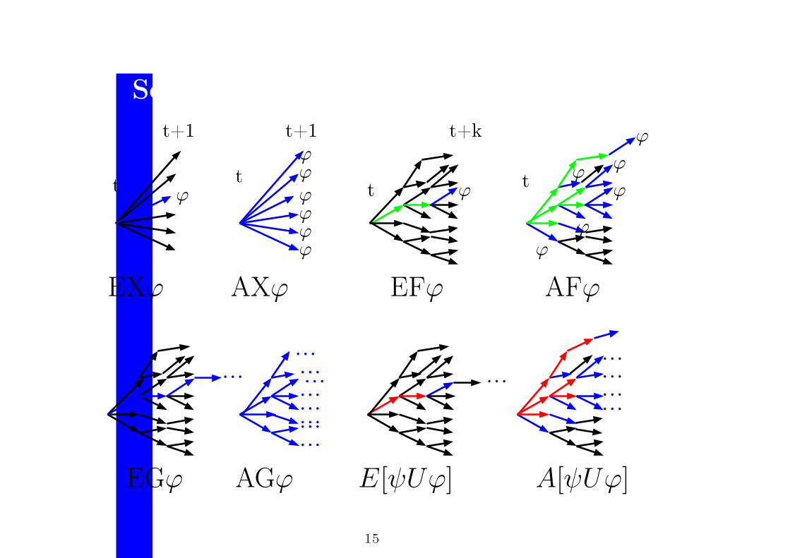
Semantics of Temporal Connectives
t+1
ϕ
AXϕ
ϕϕ
ϕϕϕ
ϕt+1
ϕ
EXϕ
t tt ϕ t
t+k
EFϕ
........................
AGϕ
...
EGϕ
...
AFϕ
ϕ
ϕϕ
ϕϕ
E[ψUϕ] A[ψUϕ]
...
...
...
...
15
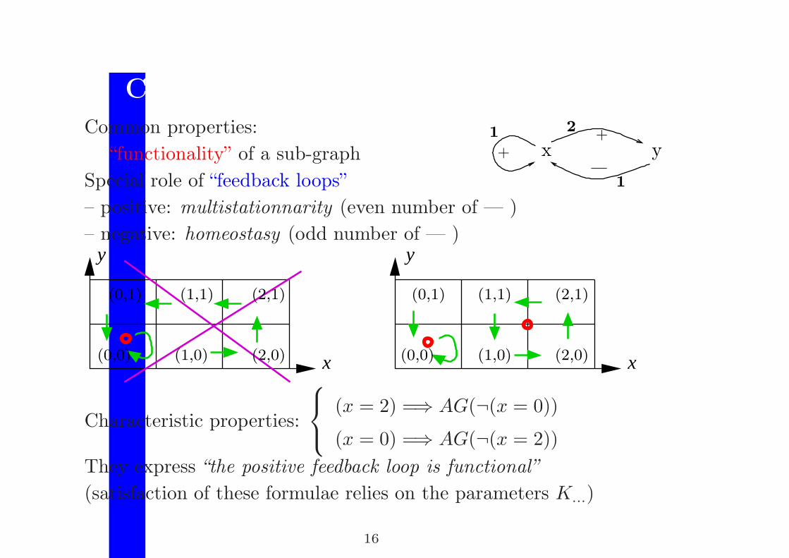
CTL to encode Biological Properties
Common properties:
“functionality” of a sub-graph
Special role of “feedback loops”—
y+
+ x1 2
1
– positive: multistationnarity (even number of — )
– negative: homeostasy (odd number of — )y
x
y
x
(0,1) (2,1)(1,1)
(2,0)(0,0) (1,0) (0,0) (1,0) (2,0)
(2,1)(1,1)(0,1)
Characteristic properties:
(x = 2) =⇒ AG(¬(x = 0))
(x = 0) =⇒ AG(¬(x = 2))
They express “the positive feedback loop is functional”
(satisfaction of these formulae relies on the parameters K...)
16
Model Checking
Efficiently computes all the states of a state graph which satisfy a
given formula: { η | M |=η ϕ }.
Efficiently select the models which globally satisfy a given formula.
17

Model Checking for CTL
Computes all the states of a theoretical model which satisfy a given
formula: { η | M |=η ϕ }.
Idea 1: work on the state graph instead of the path trees.
Idea 2: check first the atoms of ϕ and then check the connectives of
ϕ with a bottom-up computation strategy.
Idea 3: (computational optimization) group some cases together
using BDDs (Binary Decision Diagrams).
Example : (x = 0) =⇒ AG(¬(x = 2))
Obsession: travel the state graph as less as possible
18
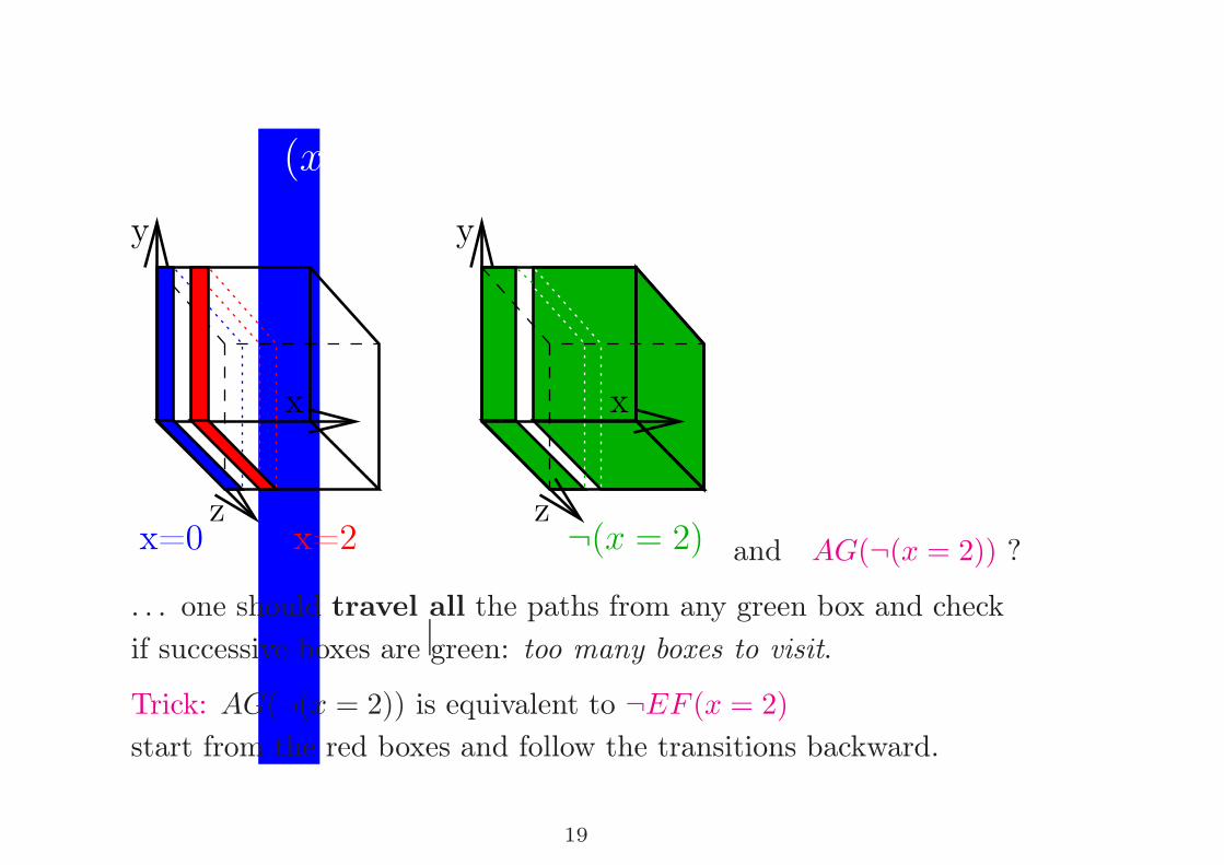
(x = 0) =⇒ AG(¬(x = 2))
x=0 x=2z¬(x = 2)
z
x
y
x
y
and AG(¬(x = 2)) ?
. . . one should travel all the paths from any green box and check
if successive boxes are green: too many boxes to visit.
Trick: AG(¬(x = 2)) is equivalent to ¬EF (x = 2)
start from the red boxes and follow the transitions backward.
19
Theoretical Models ↔ Experiments
CTL formulae are satisfied (or refuted) w.r.t. a set of paths from a
given initial state
• They can be tested against the possible paths of the theoretical
models (M |=Model Checking ϕ)
• They can be tested against the biological experiments
(Biological_Object |=Experiment ϕ)
CTL formulae link theoretical models and biological objects together
20
Menu
1. Modelling biological regulatory networks
2. Discrete framework for biological regulatory networks
3. Temporal logic and Model Checking for biology
4. Computer aided elaboration of formal models
5. Pedagogical example: Pseudomonas aeruginosa
6. Some current research topics
21
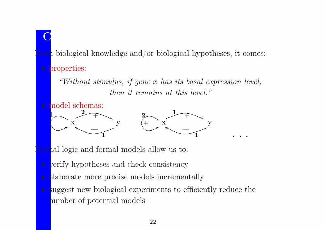
Computer Aided Elaboration of Models
From biological knowledge and/or biological hypotheses, it comes:
• properties:
“Without stimulus, if gene x has its basal expression level,
then it remains at this level.”
• model schemas:
—
y+
+ x1 2
1—
x y+
+
21
1 . . .
Formal logic and formal models allow us to:
• verify hypotheses and check consistency
• elaborate more precise models incrementally
• suggest new biological experiments to efficiently reduce the
number of potential models
22
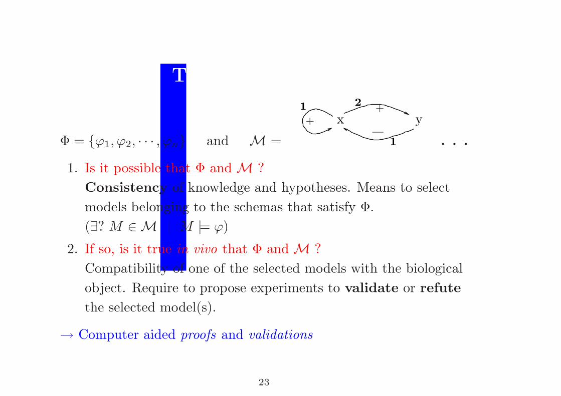
The Two Questions
Φ = {ϕ1, ϕ2, · · · , ϕn} and M =—
y+
+ x1 2
1 . . .
1. Is it possible that Φ and M ?
Consistency of knowledge and hypotheses. Means to select
models belonging to the schemas that satisfy Φ.
(∃? M ∈ M | M |= ϕ)
2. If so, is it true in vivo that Φ and M ?
Compatibility of one of the selected models with the biological
object. Require to propose experiments to validate or refute
the selected model(s).
→ Computer aided proofs and validations
23
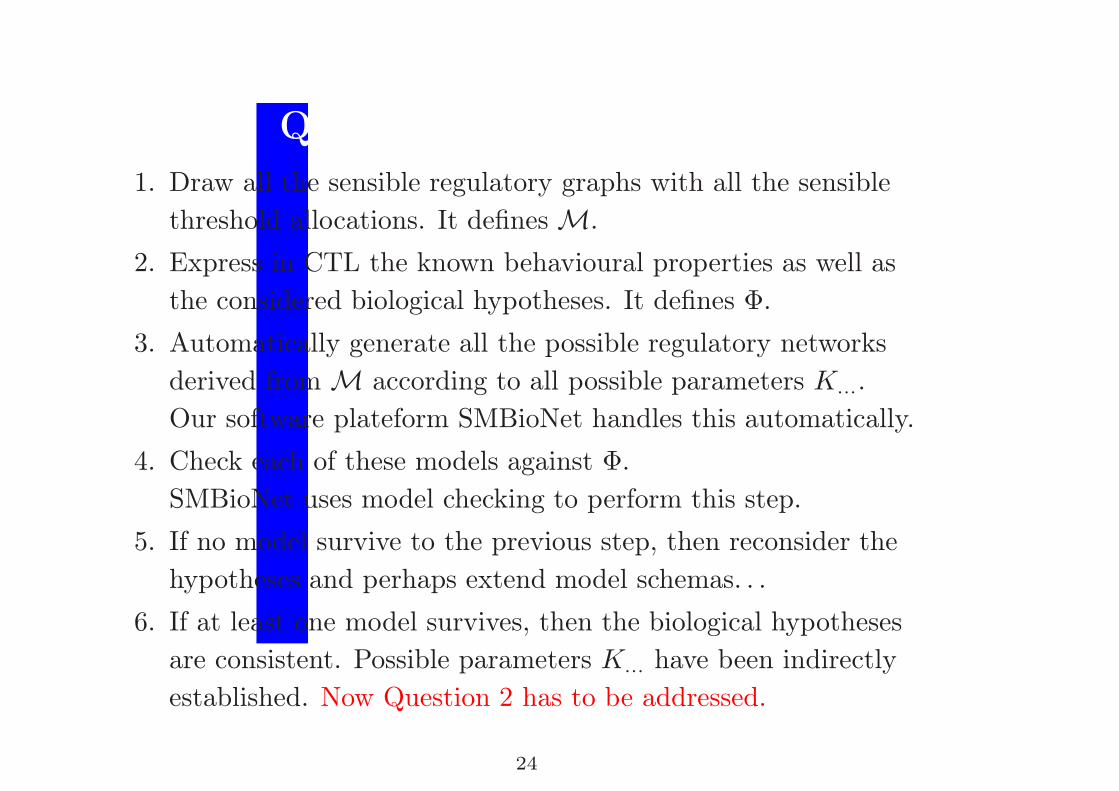
Question 1 = Consistency
1. Draw all the sensible regulatory graphs with all the sensible
threshold allocations. It defines M.
2. Express in CTL the known behavioural properties as well as
the considered biological hypotheses. It defines Φ.
3. Automatically generate all the possible regulatory networks
derived from M according to all possible parameters K....
Our software plateform SMBioNet handles this automatically.
4. Check each of these models against Φ.
SMBioNet uses model checking to perform this step.
5. If no model survive to the previous step, then reconsider the
hypotheses and perhaps extend model schemas. . .
6. If at least one model survives, then the biological hypotheses
are consistent. Possible parameters K... have been indirectly
established. Now Question 2 has to be addressed.
24
Generation of biological experiments (1)
Set of all the formulae:
ϕ = hypothesis
ϕ
25
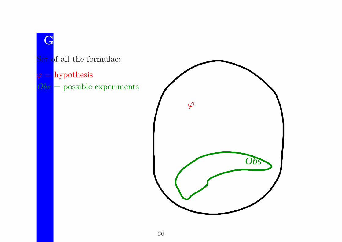
Generation of biological experiments (2)
Set of all the formulae:
ϕ = hypothesis
Obs = possible experiments
Obs
ϕ
26
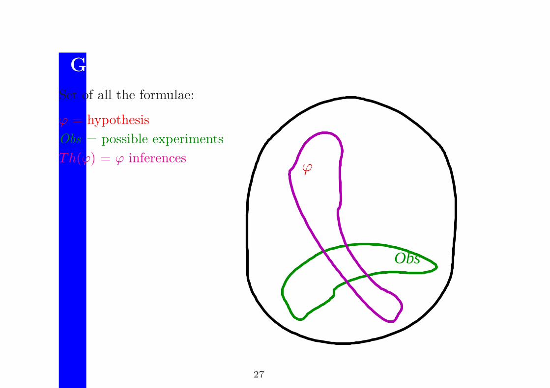
Generation of biological experiments (3)
Set of all the formulae:
ϕ = hypothesis
Obs = possible experiments
Th(ϕ) = ϕ inferences
Obs
ϕ
27
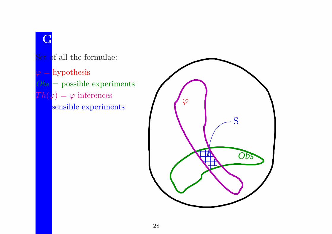
Generation of biological experiments (4)
Set of all the formulae:
ϕ = hypothesis
Obs = possible experiments
Th(ϕ) = ϕ inferences
S = sensible experiments
Obs
ϕ
S
28
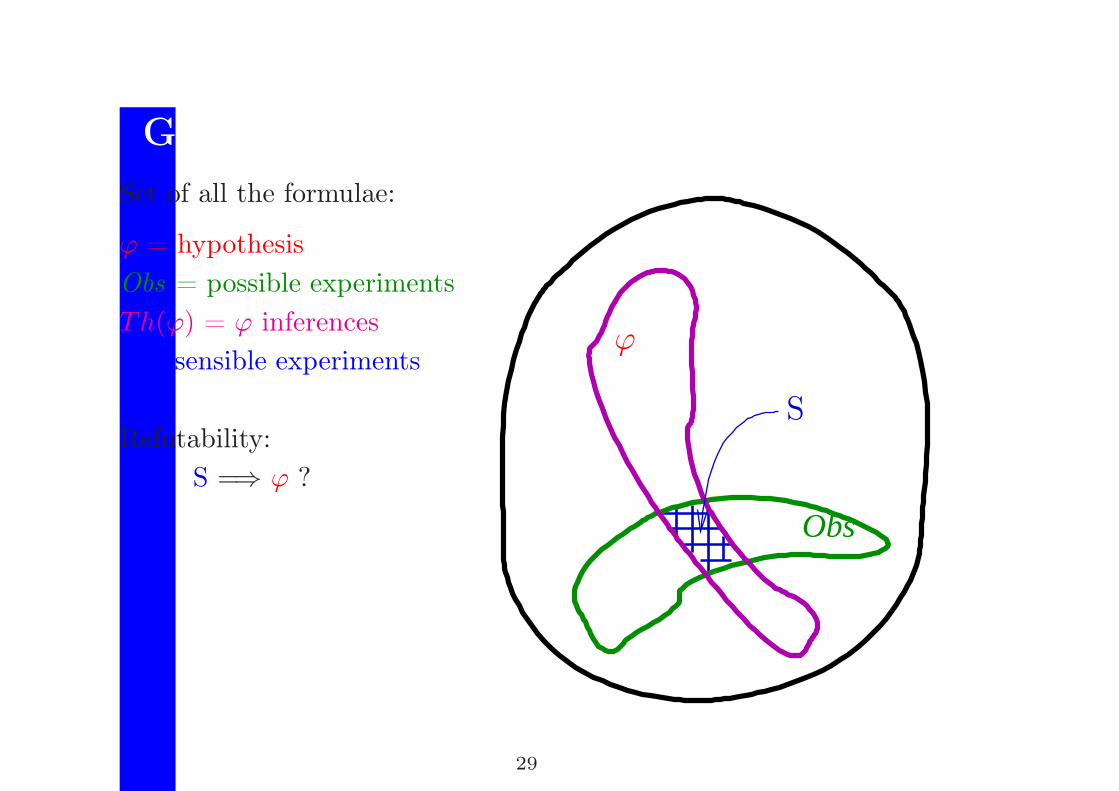
Generation of biological experiments (5)
Set of all the formulae:
ϕ = hypothesis
Obs = possible experiments
Th(ϕ) = ϕ inferences
S = sensible experiments
Refutability:
S =⇒ ϕ ?
Obs
ϕ
S
29
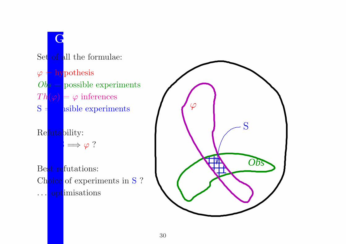
Generation of biological experiments
Set of all the formulae:
ϕ = hypothesis
Obs = possible experiments
Th(ϕ) = ϕ inferences
S = sensible experiments
Refutability:
S =⇒ ϕ ?
Best refutations:
Choice of experiments in S ?
. . . optimisations
Obs
ϕ
S
30
Question 2 = Validation
1. Among all possible formulae, some are “observable” i.e., they
express a possible result of a possible biological experiment.
Let Obs be the set of all observable formulae.
2. Let Λ be the set of theorems of Φ and M.
Λ ∩Obs is the set of experiments able to validate the survivors
of Question 1. Unfortunately it is infinite in general.
3. Testing frameworks from computer science aim at selecting a
finite subsets of these observable formulae, which maximize the
chance to refute the survivors.
4. These subsets are often too big, nevertheless these testing
frameworks can be suitably applied to regulatory networks.
It has been the case of the mucus production of P.aeruginosa.
31
Menu
1. Modelling biological regulatory networks
2. Discrete framework for biological regulatory networks
3. Temporal logic and Model Checking for biology
4. Computer aided elaboration of formal models
5. Pedagogical example: Pseudomonas aeruginosa
6. Some current research topics
32
Mutation, Epigenesis, Adaptation
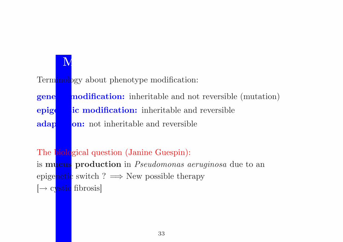
Terminology about phenotype modification:
genetic modification: inheritable and not reversible (mutation)
epigenetic modification: inheritable and reversible
adaptation: not inheritable and reversible
The biological question (Janine Guespin):
is mucus production in Pseudomonas aeruginosa due to an
epigenetic switch ? =⇒ New possible therapy
[→ cystic fibrosis]
33
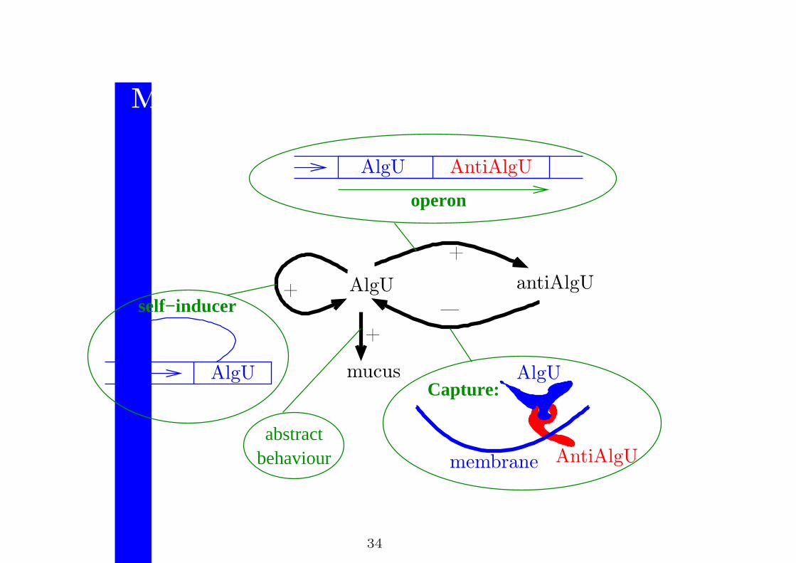
Mucus Production in P. aeruginosa
Capture:
operon
self−inducer
abstractbehaviour
—
+
AlgU antiAlgU
mucus
+
+
membrane
AlgU
AntiAlgU
AntiAlgUAlgU
AlgU
34
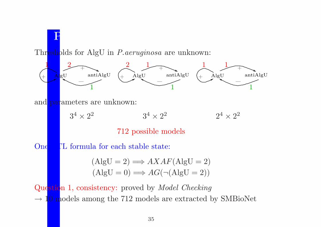
Parameters & thresholds: unknown
Thresholds for AlgU in P.aeruginosa are unknown:
—
+
+—
+
+—
+
+ antiAlgUAlgUAlgUAlgU antiAlgU antiAlgU
1 1 1
1 1 112 2
and parameters are unknown:
34 × 22 34 × 22 24 × 22
712 possible models
One CTL formula for each stable state:
(AlgU = 2) =⇒ AXAF (AlgU = 2)
(AlgU = 0) =⇒ AG(¬(AlgU = 2))
Question 1, consistency: proved by Model Checking
→ 10 models among the 712 models are extracted by SMBioNet
35

Validation of the epigenetic hypothesis
Question 2 = to validate bistationnarity in vivo
Non mucoid state: (AlgU = 0) =⇒ AG(¬(AlgU = 2))
P. aeruginosa, with a basal level for AlgU does not produce mucus
spontaneously : actually validated
Mucoid state: (AlgU = 2) =⇒ AXAF (AlgU = 2)
Experimental limitation:
AlgU can be saturated but it cannot be measured.
Experiment:
to pulse AlgU and then to test if mucus production remains
(⇐⇒ to verify a hysteresis)
This experiment can be generated automatically
36
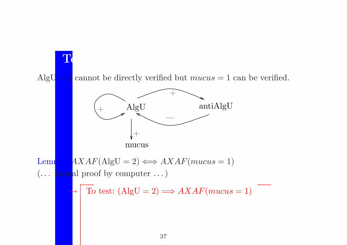
To test (AlgU=2)=⇒AXAF (AlgU=2)
AlgU = 2 cannot be directly verified but mucus = 1 can be verified.
—
+
+
AlgU antiAlgU
mucus
+
Lemma: AXAF (AlgU = 2) ⇐⇒ AXAF (mucus = 1)
(. . . formal proof by computer . . . )
→ To test: (AlgU = 2) =⇒ AXAF (mucus = 1)
37
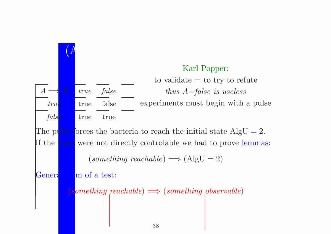
(AlgU = 2) =⇒ AXAF (mucus = 1)
A =⇒ B true false
true true false
false true true
Karl Popper:
to validate = to try to refute
thus A=false is useless
experiments must begin with a pulse
The pulse forces the bacteria to reach the initial state AlgU = 2.
If the state were not directly controlable we had to prove lemmas:
(something reachable) =⇒ (AlgU = 2)
General form of a test:
(something reachable) =⇒ (something observable)
38
Menu
1. Modelling biological regulatory networks
2. Discrete framework for biological regulatory networks
3. Temporal logic and Model Checking for biology
4. Computer aided elaboration of formal models
5. Pedagogical example: Pseudomonas aeruginosa
6. Some current research topics
39
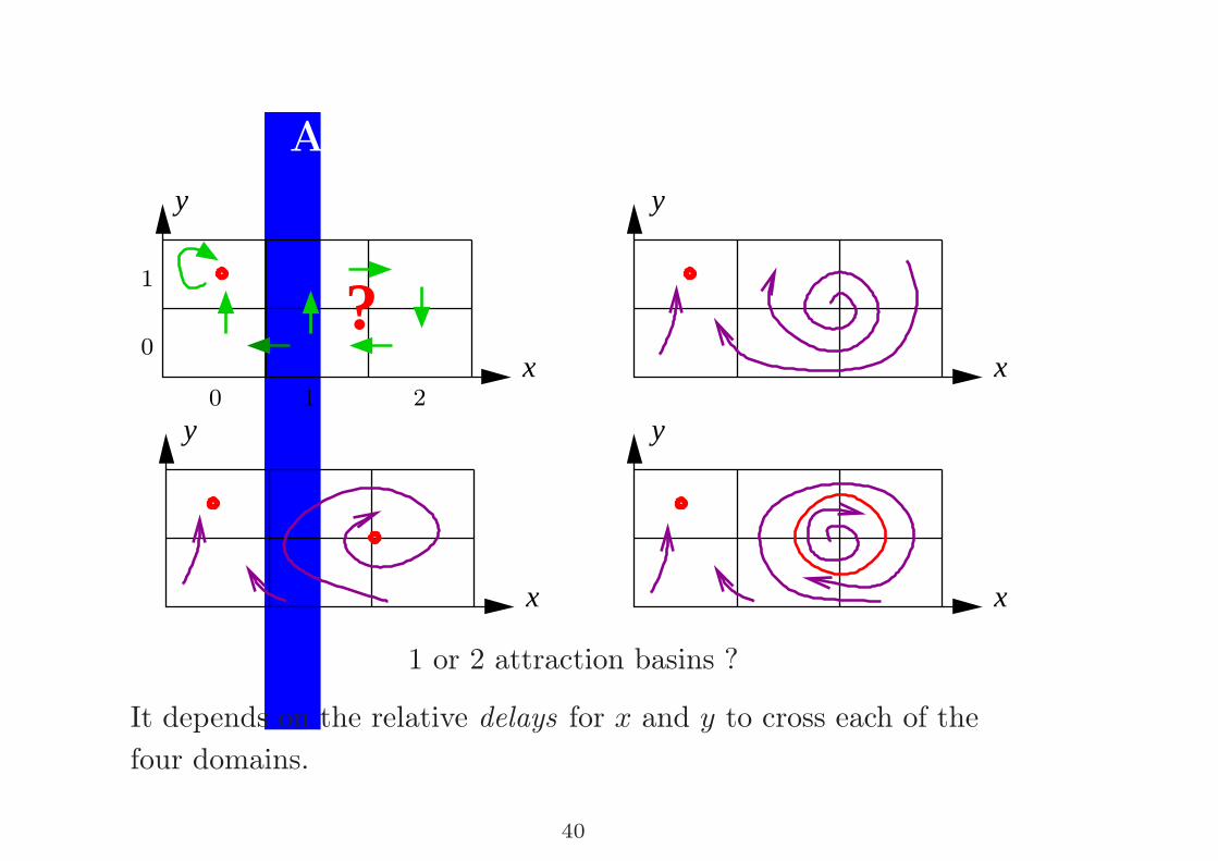
Ambiguous discrete models
y
x
y
x
y
x
y
x
?1
0
0 1 2
1 or 2 attraction basins ?
It depends on the relative delays for x and y to cross each of the
four domains.
40
Research topics (1)
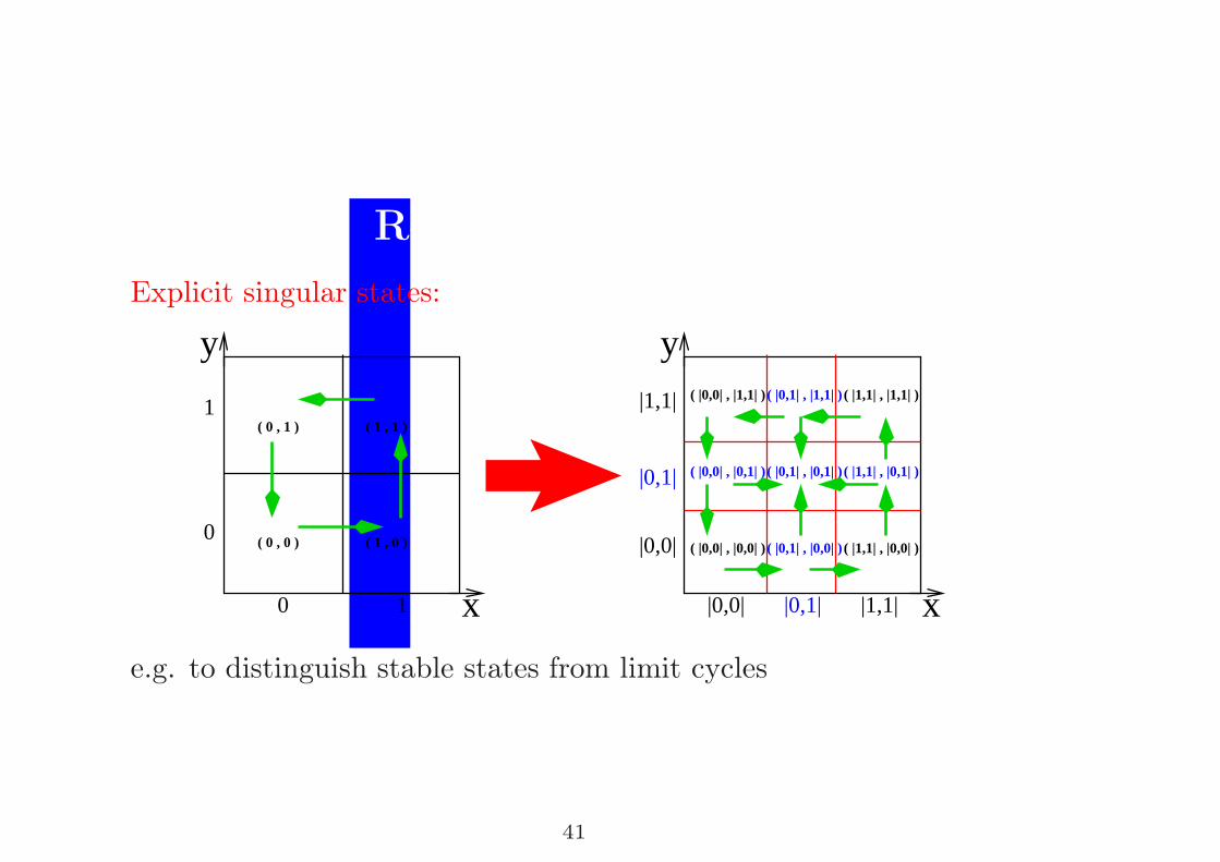
Explicit singular states:
y
0
1
0 1 x
( 1 , 0 )( 0 , 0 )
( 0 , 1 ) ( 1 , 1 )
y
x
|1,1|
|1,1|
|0,0|
|0,0|
( |0,0| , |0,0| )
( |0,0| , |0,1| )|0,1|
|0,1|
( |0,0| , |1,1| )
( |1,1| , |0,0| )
( |1,1| , |1,1| )
( |0,1| , |0,1| ) ( |1,1| , |0,1| )
( |0,1| , |0,0| )
( |0,1| , |1,1| )
e.g. to distinguish stable states from limit cycles
41
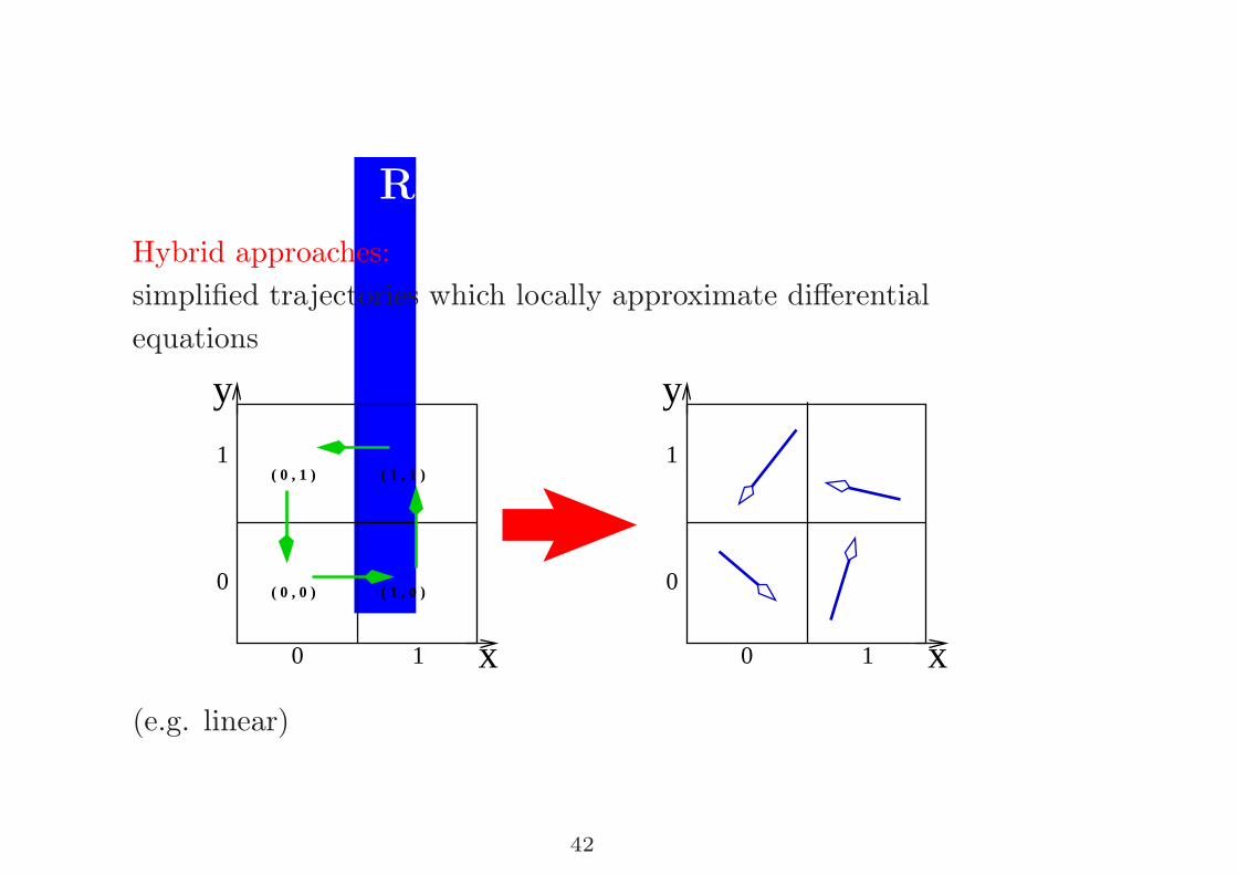
Research topics (2)
Hybrid approaches:
simplified trajectories which locally approximate differential
equations
y
0
1
0 1 x
( 1 , 0 )( 0 , 0 )
( 0 , 1 ) ( 1 , 1 )
y
0
1
0 1 x
(e.g. linear)
42
Research topics (3)
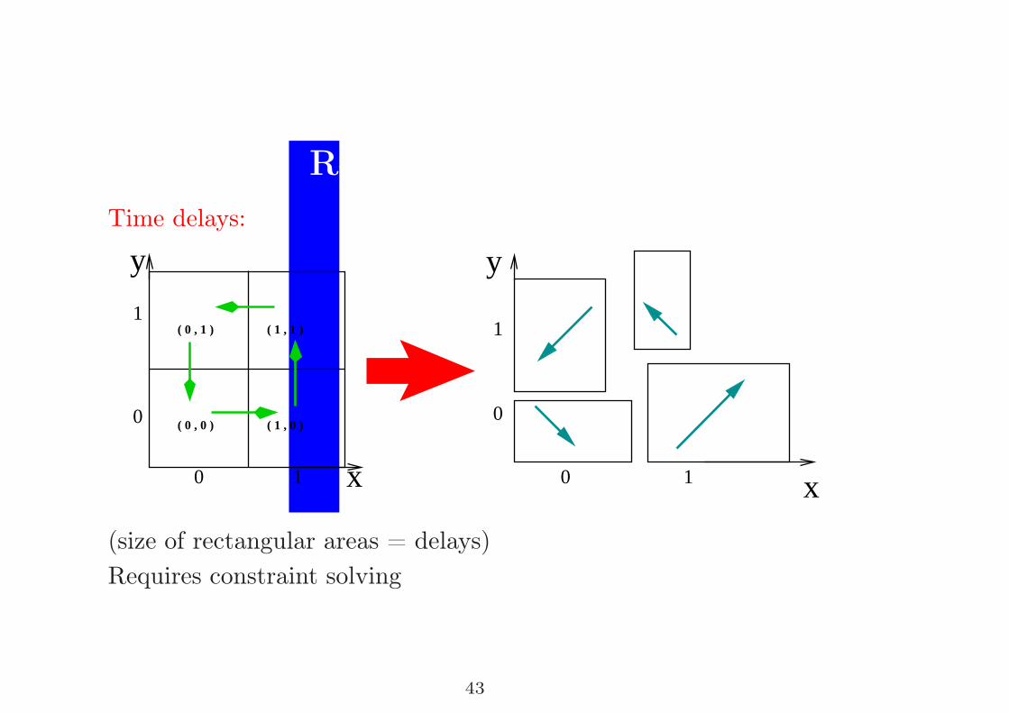
Time delays:
y
0
1
0 1 x
( 1 , 0 )( 0 , 0 )
( 0 , 1 ) ( 1 , 1 )
0 x
y
1
1
0
(size of rectangular areas = delays)
Requires constraint solving
43
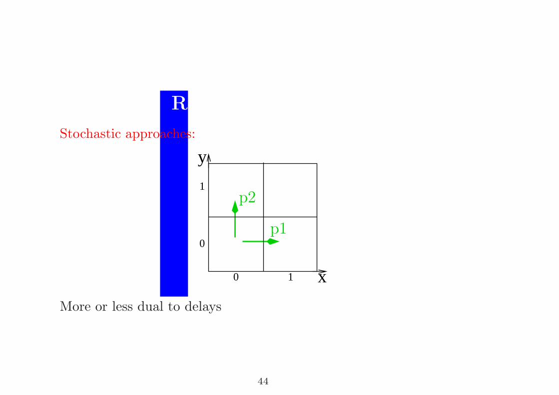
Research topics (4)
Stochastic approaches:
y
0
1
0 1 x
p1
p2
More or less dual to delays
44
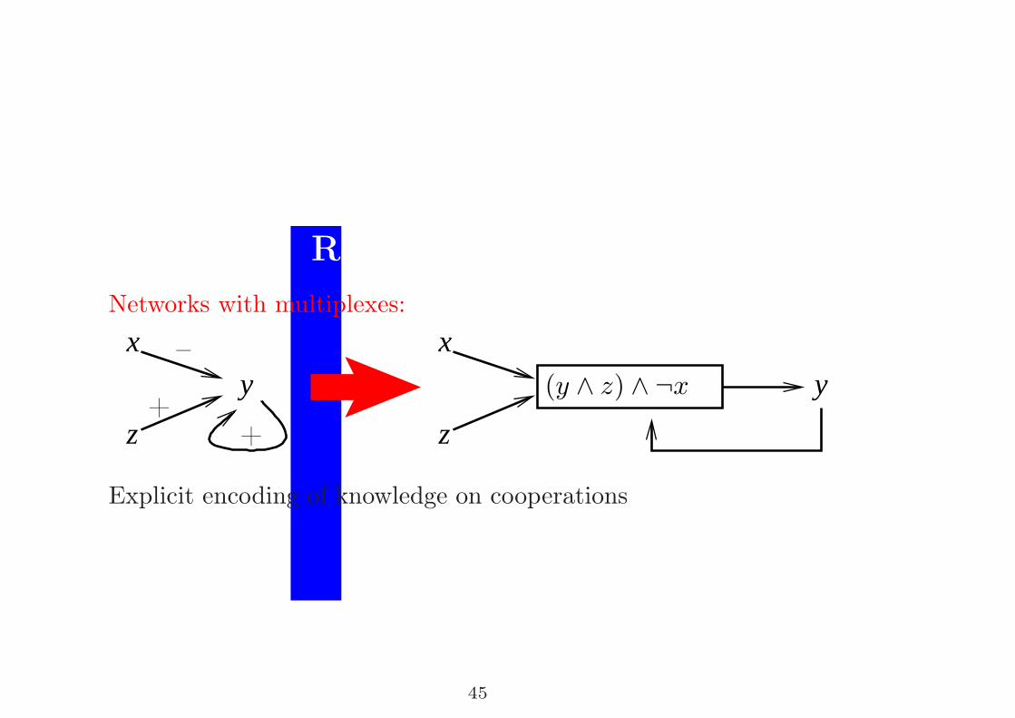
Research topics (5)
Networks with multiplexes:
y
x
z
x
z
y (y ∧ z) ∧ ¬x
–
++
Explicit encoding of knowledge on cooperations
45
Research topics (6)
From static shapes to properties on dynamics:
• positive/negative cycles and epigenesis/homeostasis
• maximum number of attraction basins
• . . .
Mathematical proofs similar to the ones for cellular automaton
46
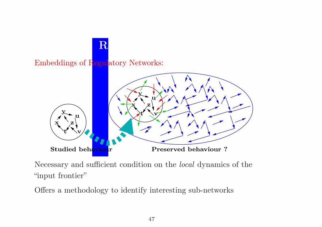
Research topics (7)
Embeddings of Regulatory Networks:
x
y
z
t
u
v
x
y
z
t
u
v
Preserved behaviour ?Studied behaviour
Necessary and sufficient condition on the local dynamics of the
“input frontier”
Offers a methodology to identify interesting sub-networks
47
Concluding Comments
Models to encode already elucidated biological models v.s.
modelling methods to help discovery in biology. . .
Behavioural properties (Φ) are as much important as models (M)
Symbolic parameter identification is essential
Modelling is significant only with respect to the considered
experimental reachability and observability (Obs)
Formal proofs can suggest wet experiments
48