Embed Size (px)
Citation preview
This research was supported by the Centre for Interna onal Finance and Regula on, which is funded by the Commonwealth and NSW Governments and supported by other Consor um members
Research Working Paper Series
Systemic Financial Risk Inference In a Global Setting Professor Jeffrey Sheen Co-Director, Centre for Financial Risk Faculty of Business and Economics Macquarie University Professor Stefan Trück Co-Director, Centre for Financial Risk Faculty of Business and Economics Macquarie University Dr Chi Truong Postdoctoral Research Fellow Faculty of Business and Economics Macquarie University Dr Ben Z Wang Lecturer Faculty of Business and Economics Macquarie University WORKING PAPER NO. 029/2014 / PROJECT NO. E034 JUNE 2014

All rights reserved. Working papers are in draft form and are distributed for purposes of comment and discussion only and may not be re-produced without permission of the copyright holder. The contents of this paper reflect the views of the author and do not represent the official views or policies of the Centre for International Finance and Regulation or any of their Consortium members. Information may be incomplete and may not be relied upon without seeking prior professional advice. The Centre for International Finance and Regulation and the Consortium partners exclude all liability arising directly or indirectly from use or reliance on the information contained in this publication
www.cifr.edu
Systemic Financial Risk Inference in a Global Setting I
Jeffrey Sheen1, Stefan Trück1, Chi Truong1, Ben Z Wang1
aFaculty of Business and Economics, Macquarie University, NSW, Australia, 2109
Abstract
We propose a new top-down approach to measure systemic risk in the financial system. Ourframework uses a combination of macroeconomic, financial and rating factors in represen-tative regions of the world. We formulate a mixed-frequency state-space model to estimatemacroeconomic factors. To derive financial risk factors, we use Moody’s/KMV expected de-fault frequencies after accounting for ratings of major financial institutions in the consideredregions. The estimated factors are combined to derive probabilities for systemically relevantdefaults in the financial industry. Regional macroeconomic factors are significant predictorsof the existence and number of systemically important defaults, while regional financial riskand ratings factors are relevant for the existence only. For major events, global credit risk alsomatters.
Keywords: Systemic financial risk, Factor models, Mixed frequency models, Kalman filter,State-space model, Hurdle modelJEL Codes: C33, E44, G01, G17.
IWe would like to thank the Australian Research Council and the Centre for International Finance and Regu-lation for providing funding support on DP 120102220 and CIFR-E034.
Email addresses: [email protected] (Jeffrey Sheen), [email protected](Stefan Trück), [email protected] (Chi Truong), [email protected] (Ben Z Wang). . July 10, 2014
1. Introduction
We introduce a new top-down approach to measure systemic risk in the financial system, com-bining information on macroeconomic, financial and ratings factors in four representative re-gions of the world. We find that regional macroeconomic conditions can predict the existenceof a systemically important financial events, as well as the number within a period. A measureof regional financial risk as well as a ratings factor are also significant predictors for the exis-tence of systemic events, and a measure of a global credit risk premium is associated with majorevents. First we formulate a state space dynamic factor model (DFM) of a variety of observedmacroeconomic and financial variables from the United States, the European Union, Australiaand China since 1990. We estimate unobserved macroeconomic factors for the ‘world’ andfor each representative region, using observed stock and flow variables arriving at mixed fre-quencies. At the next stage, these macroeconomic factors are used as drivers along with riskratings to help explain financial risks in each region, derived from Moody’s/KMV expecteddefault frequencies for major financial institutions in each region. Finally, the macroeconomic,financial and ratings factors are then combined to derive probabilities for systemically relevantdefaults in the financial industry. We then infer the evolution of systemic risks in each regionfrom these probability estimates using a hurdle model, yielding local predictions from globalinformation.
The need for a better understanding of the drivers of financial risk in a systemic context becamea major issue as a result of the recent global financial crisis in 2007 and 2008. In response tothe severe cost of the crisis, the U.S. Congress enacted the Dodd Frank Wall Street Reformand Consumer Protection Act, usually referred to as the Dodd Frank Act in July 2010. As amajor part of this reform, the Financial Stability Oversight Council (FSOC) was established toidentify risks to financial stability arising from events or activities of large financial firms orelsewhere and to respond to emerging threats to the stability of the financial system. The DoddFrank Act is evidence of the emphasis regulators put on identifying and reacting to potentialthreats of the financial system as a whole.
Research on financial crises and systemic risk has grown rapidly during the last 5 years, for ex-ample, see Ishikawa et al. (2012) for a summary of recent empirical literature and Bisias et al.(2012) for a survey on quantitative approaches to the measurement of systemic risks. Generally,the starting point for monitoring and responding to potential systemic risks is the timely andaccurate measurement of threats to the financial system. The economic and financial literatureprovides a variety of approaches to monitoring these risks, including models based on measuresof illiquidity, default risk and probability distributions, on measures created from network anal-ysis and graph-theoretic techniques, and on macroeconomic measures ((Bisias et al., 2012)).The suggested methods fall roughly into two categories: bottom-up and top-down approaches.
Bottom-up approaches in general measure the contribution of individual institutions to the sys-temic risk of the entire financial market or system in a region. They often also measure feedbackeffects between shocks to the financial system and the risk of individual financial institutions.Important representative work in this area includes Acharya et al. (2012b), Adrian and Brun-nermeier (2011), Allen et al. (2012), and Brownlees and Engle (2012), just to mention a few.
Adrian and Brunnermeier (2011) introduce the Delta Conditional Value-at-Risk (CoVaR) mea-sure, relating systemic risk to the Value-at-Risk (VaR) of the market conditional on individual
2
institutions being under distress. Similarly, Hautsch et al. (2011) measure systemic risk as thetime-varying contribution of a firm’s VaR on the market VaR, while White et al. (2012) concen-trate on spillover effects between the VaR of a financial institution and the market. Allen et al.(2012) derive a measure of aggregate systemic risk (CATFIN) using the 1% VaR measures ofa cross-section of financial firms. They suggest that the derived measure forecasts economicdownturns almost one year in advance in conducted out-of-sample tests.
Acharya et al. (2012b) measure systemic risk of a financial institution as its contribution to thetotal capital shortfall of the financial system that could be expected in a future crisis and de-rive the so-called Marginal Expected Shortfall (MES) and Systemic Expected Shortfall (SES).Following this line of thought, Acharya et al. (2012a); Brownlees and Engle (2012) propose asystemic risk measure (SRISK) that captures the expected capital shortage of a firm given itsdegree of leverage and marginal expected shortfall. Usually, these studies measure the contribu-tion of major US financial institutions to systemic risk. Note that Benoit et al. (2013) providea theoretical and empirical comparison of several of these approaches and find that differentsystemic risk measures identify very different financial institutions as being systemically im-portant. Also, their results suggest that rankings based on systemic risk estimates often mirrorrankings that could be obtained by sorting the firms based on market risk or liabilities.
Top-down approaches usually rather identify systemic risk by inferring factors relating to highlevel features of the financial system, potentially also including macroeconomic variables.Lowe and Borio (2002) and Borio and Lowe (2004) explain how systemic financial distressoften arises because financial imbalances develop in otherwise benign circumstances. For 34countries in 1960-1999, they find that sustained credit and asset price growth increased financialinstability risk. Billio et al. (2012) use principal components to analyze the interconnectednessamong hedge funds, banks, brokers, and insurance companies. They find high interrelatednessbetween these, which have become less liquid in recent years, increasing the level of systemicrisk particularly for the finance and insurance industries. Allen et al. (2010) examine the impactof networks and the architecture of the financial system on systemic risk. Schwaab et al. (2014)apply so-called coincident risk measures and early warning indicators for financial distress ofthe whole system, derived from macro and credit risk data.
In this paper we develop a top-down approach to create early warning indicators for systemicrisk. Our research design has three key elements: a global macroeconomic DFM, a global fi-nancial risk DFM, and a global systemic risk hurdle regression model.
In the first two elements, we propose DFMs for the measurement of global macroeconomic andfinancial conditions based on state space methods. In particular we estimate mixed frequencymodels to create real-time indicators of macro-financial and credit risk conditions. The appliedframework follows work by Mariano and Murasawa (2003); Aruoba et al. (2009) who applymixed-frequency models to extract factors that summarize various sources of information arriv-ing at different frequency1. Factor models and the dimension reduction of a set of explanatoryvariables have always played a substantial role in the analysis of financial markets. Applica-
1Our approach relates to the work on now-casting and real-time business and financial condition indicators.Recently, various authors have explained the importance of measuring financial and economic activity at highfrequency, for example see Altissimo et al. (2001); Evans (2005); Giannone et al. (2008); Angelini et al. (2011).In this paper, we do not restrict our attention to observable variables at the same frequency, for example, as
3
tions include, for example, asset pricing, the analysis of risk and returns, portfolio managementand modelling term structure dynamics. They allow a reduction in the dimensionality of the setof potential explanatory variables, leading to parsimonious and efficient risk management tools.DFMs have become popular in macroeconomics and finance because they provide a powerfultool for understanding the co-movement between many time series (see for example Geweke(1977), Bernanke et al. (2005), Kose et al. (2012) and Leu and Sheen (2011)). Using observedmacroeconomic and other financial variables, e.g. forward-looking measures such as impliedvolatilities, in a DFM, we estimate unobserved factors for global business cycle conditions(common to all observed variables) as well as region-specific business cycle conditions (whichare common to all observed variables in a particular region). Following a similar approach forthe second element, we use observed measures of future credit risk in the form of expected de-fault frequencies (EDFs) for a set of the top 11 financial companies in each region to estimateunobserved factors for region or country-specific financial hazards (common to all credit riskvariables in a specific region) after accounting for ratings by Moody’s and our macroeconomicfactors. These financial factor estimates deliver model-based predictors of financial distress,beyond what ratings agencies produce. The interesting question is what these model-basedpredictors can explain just before and during systemic crises, and whether they can be used tomonitor and forecast systemic risks globally or in a specific region.
Accordingly, in our third element, we delve further into early warning systems of financialstress and default, integrating our DFM factor estimates with actual default events. We con-tribute to the literature on systemic risk quantification, in particular to the area of top-downapproaches for the measurement of systemic risks in the financial system2. As complements toinformation on actual defaults and EDFs, we also include other measures of credit risk, such asfactors for credit ratings provided by Moody’s KMV and TED spreads. Since actual defaultsare relatively rare, the monthly time-series of default counts is heavily inflated by zeros. Hav-ing zero or not zero defaults in a month may well be determined by different covariates thanthe actual number of non-zero defaults. Recognizing this, a major contribution of this paper isthat we employ a hurdle model to explain the zero counts (with a Binomial process) and thenon-zero counts (with a Poisson process) using different explanatory variables. This distinctionis important because we find only recent macroeconomic history helps in explaining the sever-ity of a crisis (the number of defaults), while the financial, macroeconomic and credit ratingfactors are all important in explaining the existence of a crisis (the zeros). Also this distinctionenables us to compare the determinants of low hurdle with high hurdle crises.
in Giesecke and Kim (2011). We use data for variables that are available at different frequencies, but estimateall unobservable factors at the highest frequency of the observable data. To create an effective framework fordelivering metrics of economic activity at monthly frequency in a dynamic factor model with data on relevantvariables arriving at different frequencies, the set of information needs to be integrated using some type of efficientmultivariate filter. We apply a mixed-frequency approach with the Kalman filter as in Mariano and Murasawa(2003); Aruoba et al. (2009); Sheen et al. (2014) to integrate macroeconomic and financial variables in a coherentframework. Since this approach leads to missing data for variables at low frequencies, a state-space representationis appropriate. For the estimation of these models, the filter delivers high-frequency unobserved indicators, whichutilises efficiently information from the lower-frequency variables despite many missing data points.
2In this line of research, usually a combination of high-level features of the macro economy and the financialsystem are used to create forward-looking measures of systemic risk. Giesecke and Kim (2011) use a hazard rateapproach with contagion and additional macro-financial factors as exogenous regressors to measure systemic risk.Schwaab et al. (2014) use Moody’s credit risk data alongside macro and financial data for the US and EU (and amixture of countries for the rest of the world) to construct financial failure indicators.
4
Another contribution of our paper is that we provide a framework for measuring and analyz-ing drivers of systemic risks for the financial sector across different geographical regions usingour hurdle model. So far only a limited number of studies have focussed on an internationalor global perspective. Exceptions include the work by Pesaran et al. (2006); Schwaab et al.(2014)3. By taking an international perspective and identifying global macroeconomic and fi-nancial factors as well as links between the considered regions, the developed framework alsoallows us to retrieve information about systemic risk for regions where only limited (or evenno) information exists in default or ratings data for the financial sector. For example, for acountry like Australia, where the number of observed defaults for financial institutions is verylow and only a limited number of companies are rated by the major ratings agencies (such asMoody’s/KMV), it will be virtually impossible to derive appropriate systemic risk indicatorsfrom local data. By taking a global perspective, we can at least partially overcome this problemand assess systemic risk for such a country with limited information by taking advantage of in-ternational linkages and systematic credit risk conditions across different geographical regions.
The remainder of the paper is organized as follows. Section 2 introduces the applied frameworkfor measuring macro-economic conditions for four representative regions of the world. Section3 develops a framework for estimating regional financial risk factors based on Moody’s KMVexpected default frequencies (EDFs), beyond the roles of credit risk ratings and macroeconomicfactors. Section 4 provides empirical results on the estimation of a systemic risk index using themacroeconomic, financial risk and ratings factors. It examines the usefulness of these estimatesfor predicting systemic risk in the considered regions. Section 6 concludes.
2. The dynamic macroeconomic factor model
We formulate a state space model to estimate macroeconomic factors for different represen-tative regions of the world using macroeconomic data observed at different frequencies. Themodel is based on an extended cumulator method that allows for autoregressive processes (forexample, see Harvey (1990), Aruoba et al. (2009) and Sheen et al. (2013)). With this method,flow variables observed at a lower frequency are driven by the cumulated values of the un-observed state factors over the higher frequency observation period rather than by the statevariables themselves. The cumulated state variables (or cumulators) are augmented to the statevector, with the low frequency flow variables loading on the cumulators and the high frequencyvariables loading on state factors4.
We consider a five factor model—with four regional factors and one global factor. We modelthe world as composed of four representative regional types (R = 4): a rich super power—theUnited States (US); a super power bloc of countries—Europe (EU ) comprising 27 countries;a typical rich small open economy—Australia (AU ), that has had little experience of corporate
3Our paper is closely related to Schwaab et al. (2014). We differ in the following aspects: 1. Instead ofusing their more computational-demanding non-Gaussian state-space framework, we restrict ourselves to a linear-Gaussian framework to allow mixed frequency data. 2. Instead of using data on financial and non-financial firms,we focus on the former because we are interested in systemic financial crises. 3. We consider credit ratingsimportant for measuring financial risk, and so we estimate and use a credit rating factor to help explain actualdefaults. 4. They do not consider the zero inflation problem for defaults, and simply have a Binomial model.Instead we introduce a hurdle model. 5. We add China and Australia to our regional set outside the USA and theEU, while they use a differing mixture of other countries for defaults and macroeconomic data.
4In Appendix A, we give an example of a mixed frequency model with one stock and one flow variable.5
financial defaults in our sample period since 1990; and the rest of the emerging and developingworld represented by China (CH), which also has experienced very few defaults.
We assume that the factors driving the macroeconomic conditions in each region can be decom-posed into an unobserved global component that is common to all regions and an unobservedregional-specific component. The global factor component is assumed to follow an AR(1) pro-cess:
MWt+1 = φWMW
t +∑r
θWr Mrt + ηWt , (2.1)
while the specific factor of region r is:
M rt+1 = φrM r
t + θrWMWt + ηrt . (2.2)
where r = US,EU,AU,CH .
A cumulator for a flow variable in region r can be expressed as:
M r,ct+1 = ψrtM
r,ct +M r
t+1
= ψrtMr,ct + φrM r
t + θrWMWt + ηrt , (2.3)
where ψrt is an indicator variable, equal to 1 in periods t when low frequency variables are notobserved and 0 otherwise.//Observed variables used to estimate business cycle indices vary across studies. Output, con-sumption and investment data are used in Kose et al. (2003); employment, GDP and the termpremium are used in Aruoba et al. (2009); the term premium, hours worked, a business confi-dence index, the terms of trade, the real exchange rate, GDP and job vacancies are used in Sheenet al. (2013); GDP, industrial production, unemployment rate, industrial confidence index, pricedata (inflation, stock market returns), the term premium and residential property prices are usedin Schwaab et al. (2014). We use eight variables as detailed in Table 1. These variables covera range of characteristics: stocks and flows; monthly, quarterly and annual data; and economicactivity as well as pricing data in labour markets, product markets and asset markets.
6
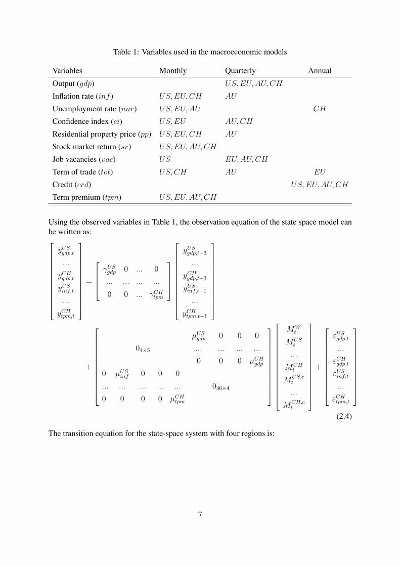
Table 1: Variables used in the macroeconomic models
Variables Monthly Quarterly Annual
Output (gdp) US,EU,AU,CH
Inflation rate (inf ) US,EU,CH AU
Unemployment rate (unr) US,EU,AU CH
Confidence index (ci) US,EU AU,CH
Residential property price (pp) US,EU,CH AU
Stock market return (sr) US,EU,AU,CH
Job vacancies (vac) US EU,AU,CH
Term of trade (tot) US,CH AU EU
Credit (crd) US,EU,AU,CH
Term premium (tpm) US,EU,AU,CH
Using the observed variables in Table 1, the observation equation of the state space model canbe written as:
yUSgdp,t
...
yCHgdp,t
yUSinf,t
...
yCHtpm,t
=
γUSgdp 0 ... 0
... ... ... ...
0 0 ... γCHtpm
yUSgdp,t−3
...
yCHgdp,t−3
yUSinf,t−1
...
yCHtpm,t−1
+
µUSgdp 0 0 0
04×5 ... ... ... ...
0 0 0 µCHgdp
0 µUSinf 0 0 0
... ... ... ... ... 036×4
0 0 0 0 µCHtpm
MWt
MUSt
...
MCHt
MUS,ct
...
MCH,ct
+
εUSgdp,t
...
εCHgdp,t
εUSinf,t
...
εCHtpm,t
(2.4)
The transition equation for the state-space system with four regions is:
7
MWt+1
MUSt+1
...
MCHt+1
MUS,ct+1
...
MCH,ct+1
=
φW θWUS θWEU θWAU θWCH 0 0 0 0
θUSW φUS 0 0 0 0 0 0 0
... ...
θCHW 0 0 0 φCH 0 0 0 0
θUSW φUS 0 0 0 ψUSt 0 0 0
... ...
θCHW 0 0 0 φCH 0 0 0 ψCHt
MWt
MUSt
...
MCHt
MUS,ct
...
MCH,ct
+
ηWt
ηUSt
...
ηCHt
ηUSt
...
ηCHt
(2.5)
For model (2.4)-(2.5) to be identified, we fix the variance of factor innovations to unity.5
2.1. Estimation resultsWe use data collected from Datastream for the period from January 1990 to December 2012.The time series for the observed variables are detrended using cubic polynomials and demeanedbefore estimation. GDP for CH and the real property prices of EU are deseasonalized using anARIMA model as suggested by the NBER.
Estimates of the 136 parameters of the model (2.4)-(2.5) are given in Table B.5 in AppendixB. As expected, we find positive loadings on GDP (not significant for CH), inflation (not sig-nificant for US and AU), business confidence, real property prices, vacancies (not significantfor EU). We find negative loadings on unemployment (not significant for CH) and the termpremium (not significant for CH), picking up the stance of monetary policy. Regarding thetransition parameters, θ and φ, all factors exhibit high persistence. The world factor is posi-tively driven by the lagged US factor, but negatively by the EU one, but the effects are small.Each region responds positively and significantly to the world factor. We find significant per-sistence of most individual data series and estimated error standard deviations.
Figure 1 presents the smoothed estimates of the world and regional macroeconomic factors,including their 95% confidence bands6. The period from the early 1990s until the mid-2000sreflect what is widely known as the ‘Great Moderation’. The world factor is only significant(and negative) during the 2008-9 financial crisis. For the US, there are three significant periods:the positive build-up from 2004 to 2007, followed by a persistent collapse into the negativezone, with a good recovery after 2011. The EU is significant (and negative) only in the crisis,obviously buoyed by the performance of the German economy. The Australian economy onlysuffers significantly for a short time in the crisis. China exhibits a significant boom in the1990s, stable (growth) in the 2000s, and just a minor and brief crisis in 2008-9.
5See Geweke and Zhou (1996) for further details about identification conditions.6At the initial period of observation, the confidence interval is typically quite large, because a diffuse prior for
the states is being used for the initial period. As soon as information becomes available, confidence shrinks to areasonable interval
8
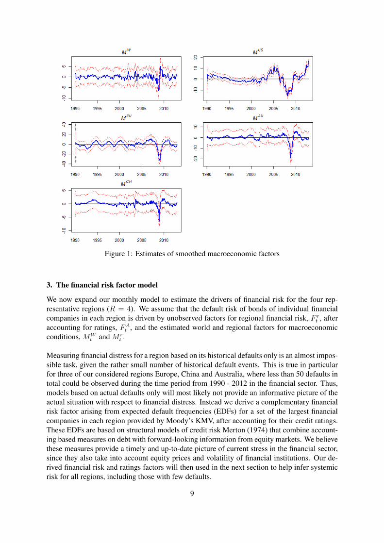
Figure 1: Estimates of smoothed macroeconomic factors
3. The financial risk factor model
We now expand our monthly model to estimate the drivers of financial risk for the four rep-resentative regions (R = 4). We assume that the default risk of bonds of individual financialcompanies in each region is driven by unobserved factors for regional financial risk, F r
t , afteraccounting for ratings, FA
t , and the estimated world and regional factors for macroeconomicconditions, MW
t and M rt .
Measuring financial distress for a region based on its historical defaults only is an almost impos-sible task, given the rather small number of historical default events. This is true in particularfor three of our considered regions Europe, China and Australia, where less than 50 defaults intotal could be observed during the time period from 1990 - 2012 in the financial sector. Thus,models based on actual defaults only will most likely not provide an informative picture of theactual situation with respect to financial distress. Instead we derive a complementary financialrisk factor arising from expected default frequencies (EDFs) for a set of the largest financialcompanies in each region provided by Moody’s KMV, after accounting for their credit ratings.These EDFs are based on structural models of credit risk Merton (1974) that combine account-ing based measures on debt with forward-looking information from equity markets. We believethese measures provide a timely and up-to-date picture of current stress in the financial sector,since they also take into account equity prices and volatility of financial institutions. Our de-rived financial risk and ratings factors will then used in the next section to help infer systemicrisk for all regions, including those with few defaults.
9
We represent each region by a set of the eleven largest financial companies (N = 11) amongMoody’s rated company bonds in that region. Credit ratings and EDFs for these companieson a monthly frequency, obtained through Moody’s KMV CreditEdge over the period 1990:1-2012.12 (T = 276), are used to estimate our financial risk factor model.
Since the EDF of company i in region r at date t, EDF ri,t, takes values between 0 and 1, we
transform it using the logistic function into a real-valued variable zri,t that is supported by aNormal distribution:
zri,t = logEDF r
i,t
100− EDF ri,t
, i = 1...N, t = 1...T, r = 1...R.
The transformed EDFs, zri,t, are assumed to depend on the Moody’s rating of company i in re-gion r at date t, the region of domicile of the company, and world and regional macroeconomicconditions:
zrit = F rt D
ri + FA
t Ari,t + κWMW
t + κrDriM
rt + εri,t, (3.1)
where Dri is an indicator variable for whether company i resides in region r, Ari,t is the rating
of company i in region r, MWt is our estimated global macroeconomic index and M r
t is ourestimated macroeconomic index of region r.7
The observation equations can be expressed in matrix form as:
zUS1,t
...
zCHN,t
=
1 ... 0 AUS1,t
... ... ... ...
0 ... 1 ACHN,t
FUSt
...
FCHt
FAt
+
MW
t MUSt ... 0
... ... ... ...
MWt 0 ... MCH
t
κW
κUS
...
κCH
+
εUS1,t
...
εCHp,t
(3.2)
We assume that the F factors evolve according to the transition equation:FUSt+1
...
FCHt+1
FAt+1
=
βUS 0 0 0 0
... ... ... ... ...
0 0 0 βCH 0
0 0 0 0 βA
FUSt
...
FCHt
FAt
+
ηUSt
...
ηCHt
ηAt
(3.3)
where the vector ηt ∼ N(0, Q), and Q is diagonal.
7The model would not be identified if both the F factors and the κ factors were time-varying. Since theestimated macroeconomic conditions indices are time-varying, we choose to keep the κs constant across time.
10

3.1. Key features of the EDF and the ratings dataFor our EDF data from Moody’s, the eleven largest financial companies in the four regions thatwe use represent 59%, 27%, 100% and 81% of the total number of bond issues and 32 %, 33 %,68 % and 38 % of the market capitalization in 2012 for the US, EU, AU and CH, respectively.In the case of China, which is a relatively new entrant to bond markets, we have also includedfinancial companies from Hong Kong8.
Bonds rather than companies are rated by Moody’s, and so multiple bond ratings may exist fora company on a single date. To obtain ratings for a company, we follow Fuertes and Kaloty-chou (2007) to use the lowest rating of senior unsecured bonds issued by that company. EDFdata are provided monthly for the period 1990-2006 and then daily thereafter. We estimate themodel using end-of-month data. Some companies may start their subscription to the ratingsservice later than others while some may cease earlier. For those that start later (or end early),we ignore their earlier (later) EDF data.
The distribution of observations across ratings are shown in Table 2. The data are more concen-trated in higher ratings with about 90% of observations for Baa1 or better. However, movementsof ratings to low levels may provide valuable information for the study of systemic risk. Theconventional approach is to group ratings together and assign a separate factor to each group.In grouping low ratings with higher ratings, the information of sudden increases in risk may belost. To preserve the information, we create a numerical ranking for assigned ratings, from 1for the highest rating Aaa to 16 for the lowest rating B3. Thus movements to low ratings willincrease the rank value. Since all ratings are considered together, a data sparsity issue does notarise.
8Since the Hong Kong and mainland Chinese economies are closely linked, our estimated CH macroeconomicfactor is likely to have similar effects on the EDFs and defaults for financial companies in both.
11
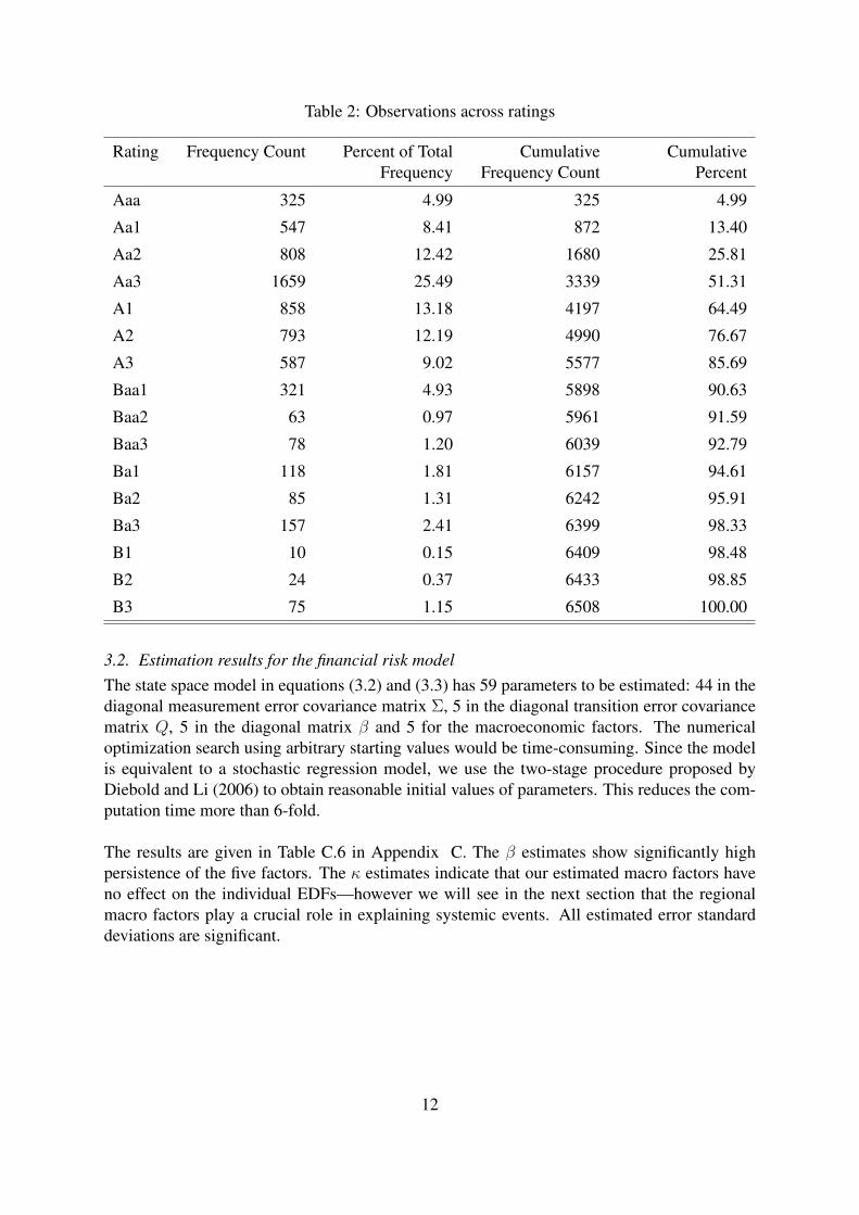
Table 2: Observations across ratings
Rating Frequency Count Percent of TotalFrequency
CumulativeFrequency Count
CumulativePercent
Aaa 325 4.99 325 4.99
Aa1 547 8.41 872 13.40
Aa2 808 12.42 1680 25.81
Aa3 1659 25.49 3339 51.31
A1 858 13.18 4197 64.49
A2 793 12.19 4990 76.67
A3 587 9.02 5577 85.69
Baa1 321 4.93 5898 90.63
Baa2 63 0.97 5961 91.59
Baa3 78 1.20 6039 92.79
Ba1 118 1.81 6157 94.61
Ba2 85 1.31 6242 95.91
Ba3 157 2.41 6399 98.33
B1 10 0.15 6409 98.48
B2 24 0.37 6433 98.85
B3 75 1.15 6508 100.00
3.2. Estimation results for the financial risk modelThe state space model in equations (3.2) and (3.3) has 59 parameters to be estimated: 44 in thediagonal measurement error covariance matrix Σ, 5 in the diagonal transition error covariancematrix Q, 5 in the diagonal matrix β and 5 for the macroeconomic factors. The numericaloptimization search using arbitrary starting values would be time-consuming. Since the modelis equivalent to a stochastic regression model, we use the two-stage procedure proposed byDiebold and Li (2006) to obtain reasonable initial values of parameters. This reduces the com-putation time more than 6-fold.
The results are given in Table C.6 in Appendix C. The β estimates show significantly highpersistence of the five factors. The κ estimates indicate that our estimated macro factors haveno effect on the individual EDFs—however we will see in the next section that the regionalmacro factors play a crucial role in explaining systemic events. All estimated error standarddeviations are significant.
12
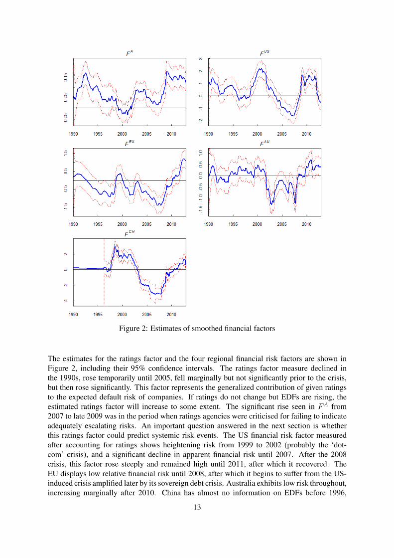
Figure 2: Estimates of smoothed financial factors
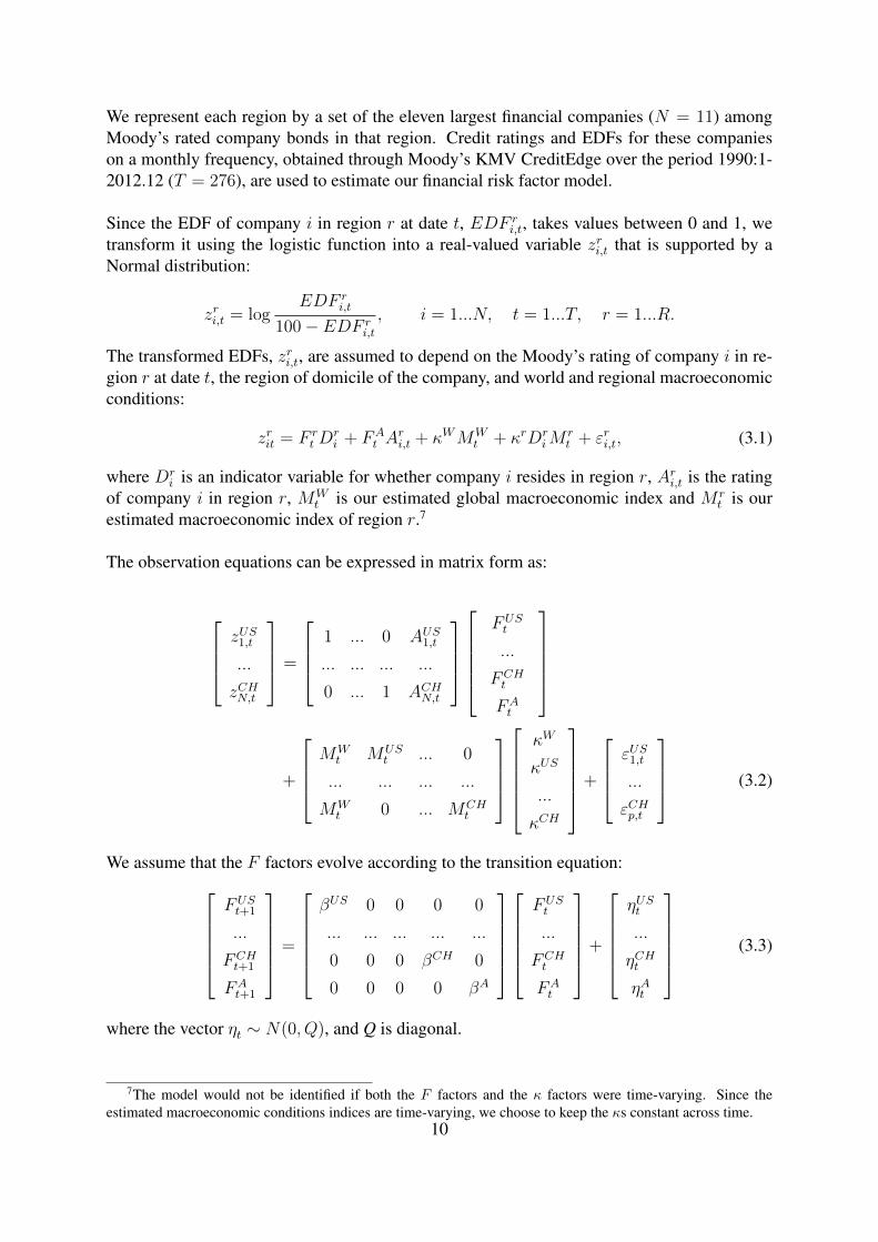
The estimates for the ratings factor and the four regional financial risk factors are shown inFigure 2, including their 95% confidence intervals. The ratings factor measure declined inthe 1990s, rose temporarily until 2005, fell marginally but not significantly prior to the crisis,but then rose significantly. This factor represents the generalized contribution of given ratingsto the expected default risk of companies. If ratings do not change but EDFs are rising, theestimated ratings factor will increase to some extent. The significant rise seen in FA from2007 to late 2009 was in the period when ratings agencies were criticised for failing to indicateadequately escalating risks. An important question answered in the next section is whetherthis ratings factor could predict systemic risk events. The US financial risk factor measuredafter accounting for ratings shows heightening risk from 1999 to 2002 (probably the ‘dot-com’ crisis), and a significant decline in apparent financial risk until 2007. After the 2008crisis, this factor rose steeply and remained high until 2011, after which it recovered. TheEU displays low relative financial risk until 2008, after which it begins to suffer from the US-induced crisis amplified later by its sovereign debt crisis. Australia exhibits low risk throughout,increasing marginally after 2010. China has almost no information on EDFs before 1996,
13
declining financial risk as its economy boomed until 2007, but a steep increase from 2008 as itfinancial system came under increasing pressure from its fast economic growth.
4. Modelling systemic indices
If a single major financial firm defaults or if a cluster of financial institutions defaults simul-taneously, this will typically unsettle confidence in the regional or even the global financialsystem. Therefore we define systemic risk as the time varying probability of sufficiently largedefaults of one or more currently active financial institutions in a given economic region duringa particular period. Such a definition of systemic risk or financial distress has been appliedin several previous studies, including, for example, Giesecke and Kim (2011); Goodhart andSegoviano (2009); Schwaab et al. (2014). In particular we define a systemically relevant eventas a default where the total market capitalization of the defaulting companies accounts for k%or more of a region’s market capitalization.9 We consider two values of k to test whether weneed to distinguish between a larger number of systemic events that also includes defaults offinancial institutions with a lower regional market capitalization effect (i.e. a smaller k), anda smaller number of larger systemic events (i.e. a larger choice of k). These two cases are la-belled ‘low hurdle’ and ‘high hurdle’ systemic events, though note that all ‘high hurdle’ eventsare contained in the set of ‘low hurdle’ events.
Information about financial defaults is extracted from Compustat and Moody’s Default RiskService (DRS). Note that Compustat records defaulted companies when they file bankruptcyunder Chapter 7 and Chapter 11, see, e.g., Duffie et al. (2007) for more details. These defaultsmay not necessarily cover all the cases of default listed in Moody’s DRS. This is due to thebroader definition of default adopted by Moody’s DRS, including three types of credit events:(1) a missed or delayed disbursement of interest and/or principal; (2) bankruptcy, administra-tion, legal receivership, or other legal blocks (perhaps by regulators) to the timely payment ofinterest and/or principal; or (3) a distressed exchange to help the borrower avoid default. Weincluded both default events recorded in Moody’s DRS and Compustat, since both definitionsof defaults are relevant for the systemic risk of the financial sector.
4.1. Features of the default data
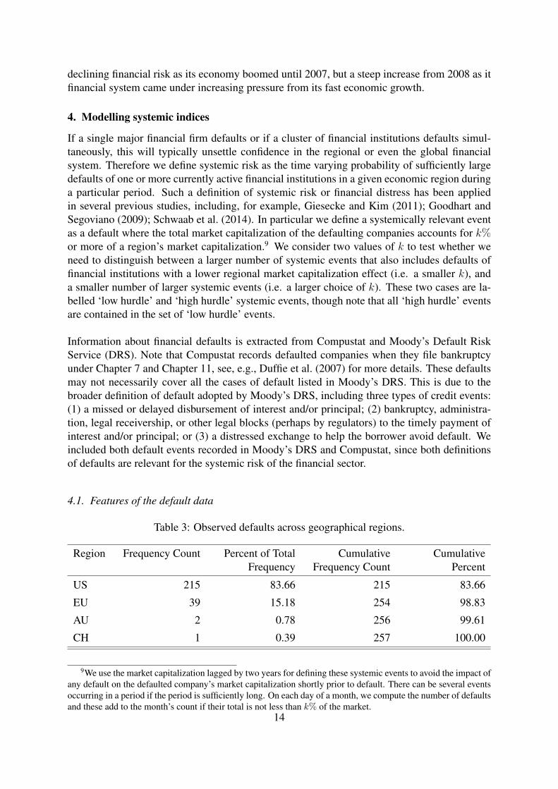
Table 3: Observed defaults across geographical regions.
Region Frequency Count Percent of TotalFrequency
CumulativeFrequency Count
CumulativePercent
US 215 83.66 215 83.66
EU 39 15.18 254 98.83
AU 2 0.78 256 99.61
CH 1 0.39 257 100.00
9We use the market capitalization lagged by two years for defining these systemic events to avoid the impact ofany default on the defaulted company’s market capitalization shortly prior to default. There can be several eventsoccurring in a period if the period is sufficiently long. On each day of a month, we compute the number of defaultsand these add to the month’s count if their total is not less than k% of the market.
14
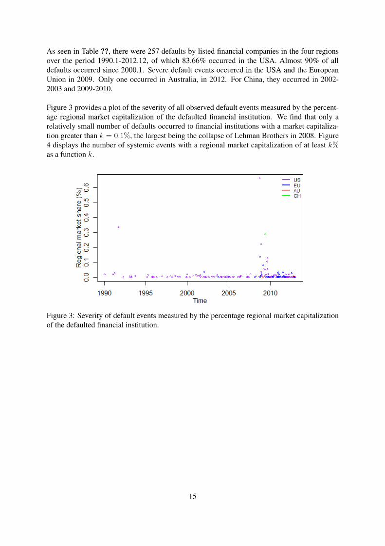
As seen in Table ??, there were 257 defaults by listed financial companies in the four regionsover the period 1990.1-2012.12, of which 83.66% occurred in the USA. Almost 90% of alldefaults occurred since 2000.1. Severe default events occurred in the USA and the EuropeanUnion in 2009. Only one occurred in Australia, in 2012. For China, they occurred in 2002-2003 and 2009-2010.
Figure 3 provides a plot of the severity of all observed default events measured by the percent-age regional market capitalization of the defaulted financial institution. We find that only arelatively small number of defaults occurred to financial institutions with a market capitaliza-tion greater than k = 0.1%, the largest being the collapse of Lehman Brothers in 2008. Figure4 displays the number of systemic events with a regional market capitalization of at least k%as a function k.
Figure 3: Severity of default events measured by the percentage regional market capitalizationof the defaulted financial institution.
15
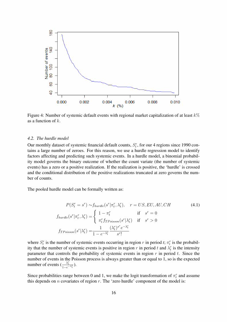
Figure 4: Number of systemic default events with regional market capitalization of at least k%as a function of k.
4.2. The hurdle modelOur monthly dataset of systemic financial default counts, Srt , for our 4 regions since 1990 con-tains a large number of zeroes. For this reason, we use a hurdle regression model to identifyfactors affecting and predicting such systemic events. In a hurdle model, a binomial probabil-ity model governs the binary outcome of whether the count variate (the number of systemicevents) has a zero or a positive realization. If the realization is positive, the ‘hurdle’ is crossedand the conditional distribution of the positive realizations truncated at zero governs the num-ber of counts.
The pooled hurdle model can be formally written as:
P (Srt = sr) ∼fhurdle(sr|πrt , λrt ), r = US,EU,AU,CH (4.1)
fhurdle(sr|πrt , λrt ) =
{1− πrt if sr = 0
πrt fTPoisson(sr|λrt ) if sr > 0
fTPoisson(sr|λrt ) =1
1− e−λrt(λrt )
sre−λrt
sr!
where Srt is the number of systemic events occurring in region r in period t; πrt is the probabil-ity that the number of systemic events is positive in region r in period t and λrt is the intensityparameter that controls the probability of systemic events in region r in period t. Since thenumber of events in the Poisson process is always greater than or equal to 1, so is the expectednumber of events ( λrt
1−e−λrt).
Since probabilities range between 0 and 1, we make the logit transformation of πrt and assumethis depends on n covariates of region r. The ‘zero hurdle’ component of the model is:
16
log πUSt /(1− πUSt )
...
log πCHt /(1− πCHt )
=
1 ZUS
1,t ZUS2,t ... ZUS
n,t
... ... ... ... ...
1 ZCH1,t ZCH
2,t ... ZCHn,t
α0
αZ1
αZ2
...
αZn
(4.2)
while for the ‘count’ component of the model, the logarithm of the Poisson parameter λrt isassumed to depend on m covariates of region r:
log λUSt
...
log λCHt
=
1 XUS
1,t XUS2,t ... XUS
m,t
... ... ... ... ...
1 XCH1,t XCH
2,t ... XCHm,t
δ0
δX1
δX2
...
δXm
(4.3)
As mentioned above, we distinguish between two different cases based on the choice of k: thecase where also ‘low hurdle’ systemic events are measured (k = 0.002%), i.e. a larger numberof defaults is included in the sample, such that we have a total of 95 systemic events for allregions. When only ‘high hurdle’ systemically relevant defaults are considered (k = 0.01%),we obtain 49 systemic events for all regions, i.e the sample contains a smaller number of moresevere default events.
The set of covariates tried in model estimation include the derived regional and world macroe-conomic factors, the regional financial risk factor, the ratings factor, a credit default spreadindex (cds), spreads between interest rates on interbank loans and on short-term governmentdebt (spread), changes in term premium (dtpm), changes in 3-month Treasury bill rate (dm3),the excess return of property price over stock market return (epp), the stock market return (sr),the volatility of stock market indices (vol), and their lags.10
4.3. Hurdle model estimatesTable 4 gives the results for the hurdle model. To reach these estimates, we began with the mostgeneral set of covariates and sequentially eliminated the most insignificant ones.
10The volatility of stock market indices is estimated using an exponentially weighted moving average (EWMA)model with λ = 0.94. The data required to calculate liquidity spreads are difficult to obtain, especially for China.Instead, we use the US TED spread for all regions since several studies have found that the TED spread drivessystemic risk not only in the USA but also in other countries. All explanatory variables are demeaned and scaledto have unit variance so that their impacts on systemic risk can be compared.
17
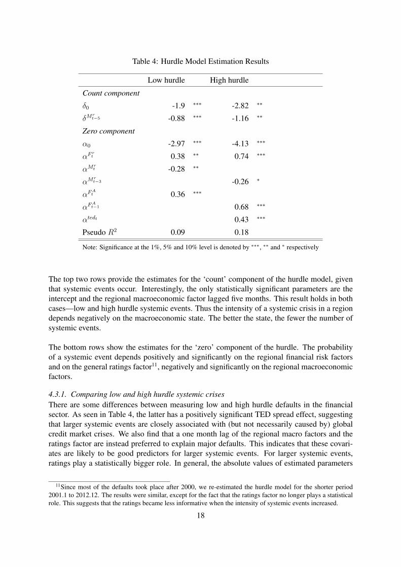
Table 4: Hurdle Model Estimation Results
Low hurdle High hurdle
Count component
δ0 -1.9 ∗∗∗ -2.82 ∗∗
δMrt−5 -0.88 ∗∗∗ -1.16 ∗∗
Zero component
α0 -2.97 ∗∗∗ -4.13 ∗∗∗
αFrt 0.38 ∗∗ 0.74 ∗∗∗
αMrt -0.28 ∗∗
αMrt−3 -0.26 ∗
αFAt 0.36 ∗∗∗
αFAt−1 0.68 ∗∗∗
αtedt 0.43 ∗∗∗
Pseudo R2 0.09 0.18
Note: Significance at the 1%, 5% and 10% level is denoted by ∗∗∗, ∗∗ and ∗ respectively
The top two rows provide the estimates for the ‘count’ component of the hurdle model, giventhat systemic events occur. Interestingly, the only statistically significant parameters are theintercept and the regional macroeconomic factor lagged five months. This result holds in bothcases—low and high hurdle systemic events. Thus the intensity of a systemic crisis in a regiondepends negatively on the macroeconomic state. The better the state, the fewer the number ofsystemic events.
The bottom rows show the estimates for the ‘zero’ component of the hurdle. The probabilityof a systemic event depends positively and significantly on the regional financial risk factorsand on the general ratings factor11, negatively and significantly on the regional macroeconomicfactors.
4.3.1. Comparing low and high hurdle systemic crisesThere are some differences between measuring low and high hurdle defaults in the financialsector. As seen in Table 4, the latter has a positively significant TED spread effect, suggestingthat larger systemic events are closely associated with (but not necessarily caused by) globalcredit market crises. We also find that a one month lag of the regional macro factors and theratings factor are instead preferred to explain major defaults. This indicates that these covari-ates are likely to be good predictors for larger systemic events. For larger systemic events,ratings play a statistically bigger role. In general, the absolute values of estimated parameters
11Since most of the defaults took place after 2000, we re-estimated the hurdle model for the shorter period2001.1 to 2012.12. The results were similar, except for the fact that the ratings factor no longer plays a statisticalrole. This suggests that the ratings became less informative when the intensity of systemic events increased.
18
are greater for high hurdle events, while the regional macro factor is marginally less significantfor major defaults in the financial sector. The (McFadden) pseudo R2 is larger for the highhurdle case, but this statistic cannot be used to compare estimations with different datasets.
For each region and crisis case, we present in Figures 5 to 12 the actual number of systemicevents, the estimated probability of a systemic event (πrt ) and the estimated number of systemicevents(πrtλ
rt/(1− e−λ
rt ). Conditional on the number of systemic events being positive, λrt/(1−
e−λrt ) is the expected number of systemic events, which must be greater than or equal to 1. The
expected number of systemic events (πrtλrt/(1−e−λ
rt ) is thus always larger than the probability
of a systemic event (πrt ) and the larger the difference, the more likely that multiple systemicevents will occur in the period. For low hurdle crises that have many more events than highhurdle crises, the difference can be and is noticeable.
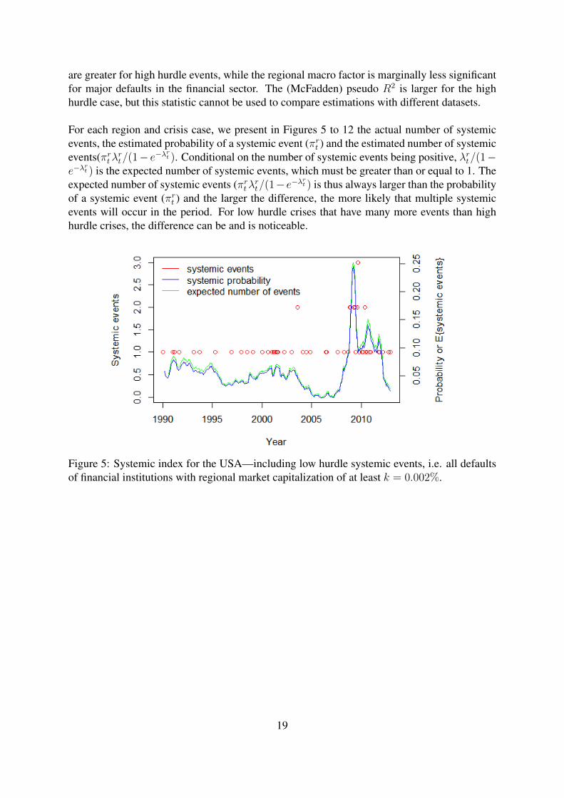
Figure 5: Systemic index for the USA—including low hurdle systemic events, i.e. all defaultsof financial institutions with regional market capitalization of at least k = 0.002%.
19
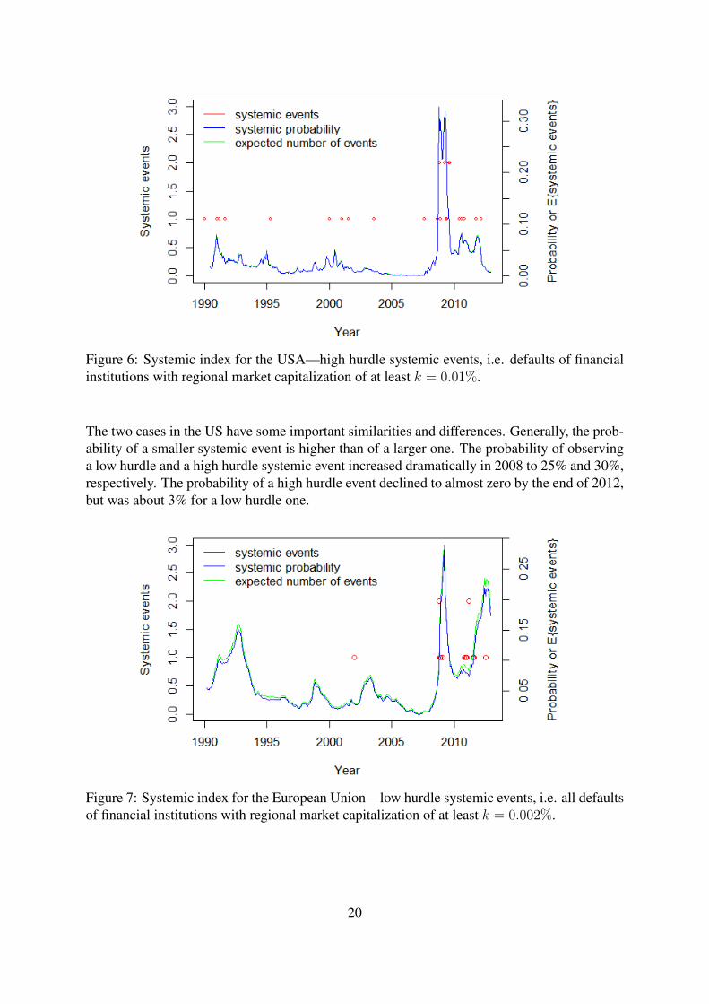
Figure 6: Systemic index for the USA—high hurdle systemic events, i.e. defaults of financialinstitutions with regional market capitalization of at least k = 0.01%.
The two cases in the US have some important similarities and differences. Generally, the prob-ability of a smaller systemic event is higher than of a larger one. The probability of observinga low hurdle and a high hurdle systemic event increased dramatically in 2008 to 25% and 30%,respectively. The probability of a high hurdle event declined to almost zero by the end of 2012,but was about 3% for a low hurdle one.
Figure 7: Systemic index for the European Union—low hurdle systemic events, i.e. all defaultsof financial institutions with regional market capitalization of at least k = 0.002%.
20
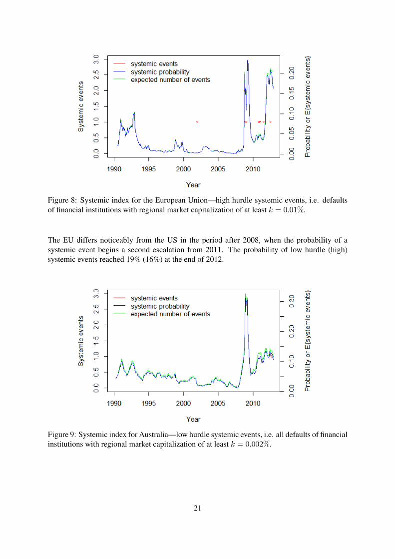
Figure 8: Systemic index for the European Union—high hurdle systemic events, i.e. defaultsof financial institutions with regional market capitalization of at least k = 0.01%.
The EU differs noticeably from the US in the period after 2008, when the probability of asystemic event begins a second escalation from 2011. The probability of low hurdle (high)systemic events reached 19% (16%) at the end of 2012.
Figure 9: Systemic index for Australia—low hurdle systemic events, i.e. all defaults of financialinstitutions with regional market capitalization of at least k = 0.002%.
21
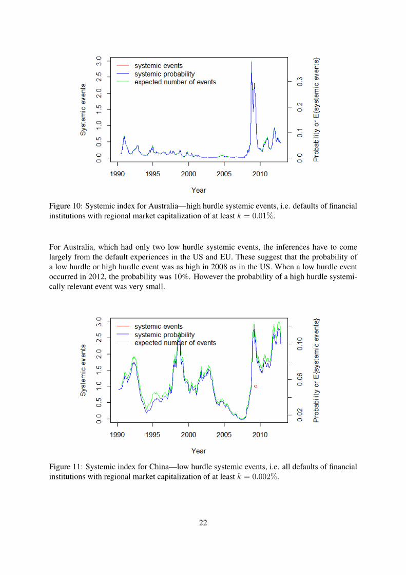
Figure 10: Systemic index for Australia—high hurdle systemic events, i.e. defaults of financialinstitutions with regional market capitalization of at least k = 0.01%.
For Australia, which had only two low hurdle systemic events, the inferences have to comelargely from the default experiences in the US and EU. These suggest that the probability ofa low hurdle or high hurdle event was as high in 2008 as in the US. When a low hurdle eventoccurred in 2012, the probability was 10%. However the probability of a high hurdle systemi-cally relevant event was very small.
Figure 11: Systemic index for China—low hurdle systemic events, i.e. all defaults of financialinstitutions with regional market capitalization of at least k = 0.002%.
22
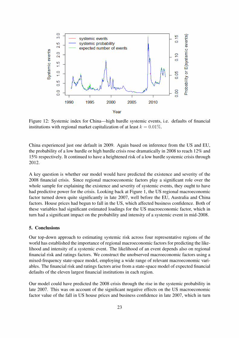
Figure 12: Systemic index for China—high hurdle systemic events, i.e. defaults of financialinstitutions with regional market capitalization of at least k = 0.01%.
China experienced just one default in 2009. Again based on inference from the US and EU,the probability of a low hurdle or high hurdle crisis rose dramatically in 2008 to reach 12% and15% respectively. It continued to have a heightened risk of a low hurdle systemic crisis through2012.
A key question is whether our model would have predicted the existence and severity of the2008 financial crisis. Since regional macroeconomic factors play a significant role over thewhole sample for explaining the existence and severity of systemic events, they ought to havehad predictive power for the crisis. Looking back at Figure 1, the US regional macroeconomicfactor turned down quite significantly in late 2007, well before the EU, Australia and Chinafactors. House prices had begun to fall in the US, which affected business confidence. Both ofthese variables had significant estimated loadings for the US macroeconomic factor, which inturn had a significant impact on the probability and intensity of a systemic event in mid-2008.
5. Conclusions
Our top-down approach to estimating systemic risk across four representative regions of theworld has established the importance of regional macroeconomic factors for predicting the like-lihood and intensity of a systemic event. The likelihood of an event depends also on regionalfinancial risk and ratings factors. We construct the unobserved macroeconomic factors using amixed-frequency state-space model, employing a wide range of relevant macroeconomic vari-ables. The financial risk and ratings factors arise from a state-space model of expected financialdefaults of the eleven largest financial institutions in each region.
Our model could have predicted the 2008 crisis through the rise in the systemic probability inlate 2007. This was on account of the significant negative effects on the US macroeconomicfactor value of the fall in US house prices and business confidence in late 2007, which in turn
23
significantly increased the probability and intensity of a systemic event in mid-2008.
Stronger macroeconomic conditions will reduce the probability and intensity of a systemicevent, both low hurdle and high hurdle ones. Policymakers need to ensure macroeconomicstability over the longer term to avoid any systemic crises. Ratings are relevant for predict-ing systemic events, but are insufficient. Just prior to the 2008 crisis, that insufficiency waspronounced. After accounting for ratings, the residual financial risk in a region arising out ofMoody’s KMV expected default frequency data is an important predictor of the probability of asystemic event. Therefore, financial regulators and supervisors need to ensure that these finan-cial risk factors are not escalating. Credit market dysfunction represented by the TED spreadis closely associated with high hurdle systemic financial crises. Therefore this indicator is auseful bellwether of a major systemic event.
24
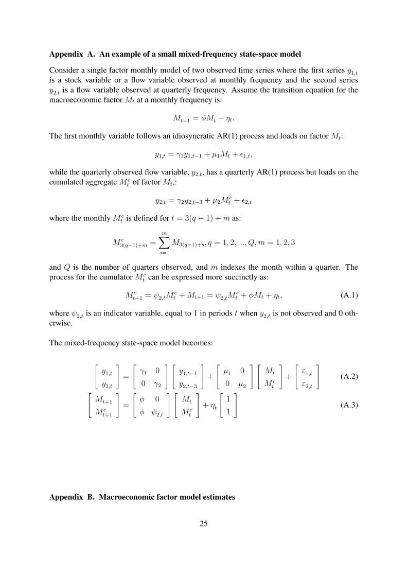
Appendix A. An example of a small mixed-frequency state-space model
Consider a single factor monthly model of two observed time series where the first series y1,tis a stock variable or a flow variable observed at monthly frequency and the second seriesy2,t is a flow variable observed at quarterly frequency. Assume the transition equation for themacroeconomic factor Mt at a monthly frequency is:
Mt+1 = φMt + ηt.
The first monthly variable follows an idiosyncratic AR(1) process and loads on factor Mt:
y1,t = γ1y1,t−1 + µ1Mt + ε1,t,
while the quarterly observed flow variable, y2,t, has a quarterly AR(1) process but loads on thecumulated aggregate M c
t of factor Mt,:
y2,t = γ2y2,t−3 + µ2Mct + ε2,t
where the monthly M ct is defined for t = 3(q − 1) +m as:
M c3(q−1)+m =
m∑s=1
M3(q−1)+s, q = 1, 2, ..., Q,m = 1, 2, 3
and Q is the number of quarters observed, and m indexes the month within a quarter. Theprocess for the cumulator M c
t can be expressed more succinctly as:
M ct+1 = ψ2,tM
ct +Mt+1 = ψ2,tM
ct + φMt + ηt, (A.1)
where ψ2,t is an indicator variable, equal to 1 in periods t when y2,t is not observed and 0 oth-erwise.
The mixed-frequency state-space model becomes:
[y1,t
y2,t
]=
[γ1 0
0 γ2
][y1,t−1
y2,t−3
]+
[µ1 0
0 µ2
][Mt
M ct
]+
[ε1,t
ε2,t
](A.2)[
Mt+1
M ct+1
]=
[φ 0
φ ψ2,t
][Mt
M ct
]+ ηt
[1
1
](A.3)
.
.
.
.
.
Appendix B. Macroeconomic factor model estimates
.25
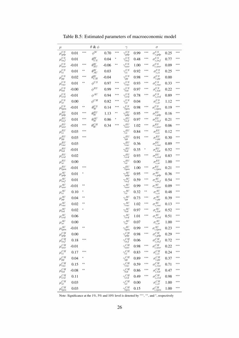
Table B.5: Estimated parameters of macroeconomic model
µ θ & φ γ σ
µUSgdp 0.01 ∗∗∗ φW 0.70 ∗∗∗ γUSgdp 0.99 ∗∗∗ σUSε,gdp 0.25 ∗∗∗
µUSinf 0.01 θWUS 0.04 ∗ γUSinf 0.48 ∗∗∗ σUSε,inf 0.77 ∗∗∗
µUSunr -0.01 ∗∗∗ θWEU -0.06 ∗∗ γUSunr 1.00 ∗∗∗ σUSε,unr 0.09 ∗∗∗
µUSci 0.01 ∗∗ θWAU 0.03 γUSci 0.92 ∗∗∗ σUSε,ci 0.25 ∗∗∗
µUSpp 0.02 ∗∗∗ θWCH -0.04 γUSpp 0.98 ∗∗∗ σUSε,pp 0.00
µUSvac 0.01 ∗∗ φUS 0.97 ∗∗∗ γUSvac 0.93 ∗∗∗ σUSε,vac 0.33 ∗∗∗
µUStot -0.00 φEU 0.99 ∗∗∗ γUStot 0.97 ∗∗∗ σUSε,tot 0.22 ∗∗∗
µUScrd -0.01 φAU 0.94 ∗∗∗ γUScrd 0.78 ∗∗∗ σUSε,crd 0.89 ∗∗∗
µUSsr 0.00 φCH 0.82 ∗∗∗ γUSsr 0.04 σUSε,sr 1.12 ∗∗∗
µUStpm -0.01 ∗∗ θUSW 0.14 ∗∗∗ γUStpm 0.98 ∗∗∗ σUSε,tpm 0.19 ∗∗∗
µEUgdp 0.01 ∗∗∗ θEUW 1.13 ∗∗ γEUgdp 0.95 ∗∗∗ σEUε,gdp 0.16 ∗∗∗
µEUinf 0.01 ∗∗∗ θAUW 0.86 ∗ γEUinf 0.97 ∗∗∗ σEUε,inf 0.21 ∗∗∗
µEUunr -0.01 ∗∗∗ θCHW 0.34 ∗∗∗ γEUunr 1.02 ∗∗∗ σEUε,unr 0.06 ∗∗∗
µEUci 0.03 ∗∗∗ γEUci 0.84 ∗∗∗ σEUε,ci 0.12 ∗∗∗
µEUpp 0.03 ∗∗∗ γEUpp 0.91 ∗∗∗ σEUε,pp 0.30 ∗∗∗
µEUvac 0.03 γEUvac 0.36 σEUε,vac 0.89 ∗∗∗
µEUtot -0.01 γEUtot 0.35 ∗ σEUε,tot 0.52 ∗∗∗
µEUcrd 0.02 γEUcrd 0.93 ∗∗∗ σEUε,crd 0.83 ∗∗∗
µEUsr 0.00 γEUsr 0.00 σEUε,sr 1.00 ∗∗∗
µEUtpm -0.01 ∗∗∗ γEUtpm 1.00 ∗∗∗ σEUε,tpm 0.21 ∗∗∗
µAUgdp 0.01 ∗ γAUgdp 0.95 ∗∗∗ σAUε,gdp 0.36 ∗∗∗
µAUinf 0.01 γAUinf 0.59 ∗∗∗ σAUε,inf 0.54 ∗∗∗
µAUunr -0.01 ∗∗ γAUunr 0.99 ∗∗∗ σAUε,unr 0.09 ∗∗∗
µAUci 0.10 ∗ γAUci 0.32 ∗∗ σAUε,ci 0.48 ∗∗∗
µAUpp 0.04 ∗∗ γAUpp 0.73 ∗∗∗ σAUε,pp 0.39 ∗∗∗
µAUvac 0.02 ∗∗ γAUvac 1.02 ∗∗∗ σAUε,vac 0.13 ∗∗∗
µAUtot 0.02 ∗ γAUtot 0.97 ∗∗∗ σAUε,tot 0.52 ∗∗∗
µAUcrd 0.06 γAUcrd 1.01 ∗∗∗ σAUε,crd 0.51 ∗∗∗
µAUsr 0.00 γAUsr 0.07 σAUε,sr 1.00 ∗∗∗
µAUtpm -0.01 ∗∗ γAUtpm 0.99 ∗∗∗ σAUε,tpm 0.23 ∗∗∗
µCHgdp 0.00 γCHgdp 0.98 ∗∗∗ σCHε,gdp 0.29 ∗∗∗
µCHinf 0.18 ∗∗∗ γCHinf 0.06 σCHε,inf 0.72 ∗∗∗
µCHunr -0.01 γCHunr 0.98 ∗∗∗ σCHε,unr 0.22 ∗∗∗
µCHci 0.17 ∗∗∗ γCHci 0.83 ∗∗∗ σCHε,ci 0.24 ∗∗∗
µCHpp 0.04 ∗ γCHpp 0.89 ∗∗∗ σCHε,pp 0.37 ∗∗∗
µCHvac 0.15 ∗∗ γCHvac 0.59 ∗∗∗ σCHε,vac 0.71 ∗∗∗
µCHtot -0.08 ∗∗ γCHtot 0.86 ∗∗∗ σCHε,tot 0.47 ∗∗∗
µCHcrd 0.11 γCHcrd 0.49 ∗∗∗ σCHε,crd 0.98 ∗∗∗
µCHsr 0.03 γCHsr 0.00 σCHε,sr 1.00 ∗∗∗
µCHtpm 0.03 γCHtpm 0.15 σCHε,tpm 1.00 ∗∗∗
Note: Significance at the 1%, 5% and 10% level is denoted by ∗∗∗, ∗∗, and ∗, respectively
26
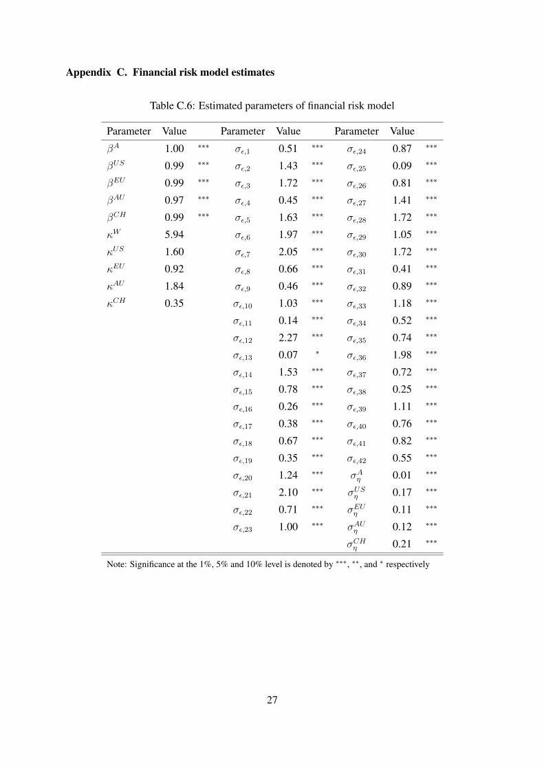
Appendix C. Financial risk model estimates
Table C.6: Estimated parameters of financial risk model
Parameter Value Parameter Value Parameter Value
βA 1.00 ∗∗∗ σε,1 0.51 ∗∗∗ σε,24 0.87 ∗∗∗
βUS 0.99 ∗∗∗ σε,2 1.43 ∗∗∗ σε,25 0.09 ∗∗∗
βEU 0.99 ∗∗∗ σε,3 1.72 ∗∗∗ σε,26 0.81 ∗∗∗
βAU 0.97 ∗∗∗ σε,4 0.45 ∗∗∗ σε,27 1.41 ∗∗∗
βCH 0.99 ∗∗∗ σε,5 1.63 ∗∗∗ σε,28 1.72 ∗∗∗
κW 5.94 σε,6 1.97 ∗∗∗ σε,29 1.05 ∗∗∗
κUS 1.60 σε,7 2.05 ∗∗∗ σε,30 1.72 ∗∗∗
κEU 0.92 σε,8 0.66 ∗∗∗ σε,31 0.41 ∗∗∗
κAU 1.84 σε,9 0.46 ∗∗∗ σε,32 0.89 ∗∗∗
κCH 0.35 σε,10 1.03 ∗∗∗ σε,33 1.18 ∗∗∗
σε,11 0.14 ∗∗∗ σε,34 0.52 ∗∗∗
σε,12 2.27 ∗∗∗ σε,35 0.74 ∗∗∗
σε,13 0.07 ∗ σε,36 1.98 ∗∗∗
σε,14 1.53 ∗∗∗ σε,37 0.72 ∗∗∗
σε,15 0.78 ∗∗∗ σε,38 0.25 ∗∗∗
σε,16 0.26 ∗∗∗ σε,39 1.11 ∗∗∗
σε,17 0.38 ∗∗∗ σε,40 0.76 ∗∗∗
σε,18 0.67 ∗∗∗ σε,41 0.82 ∗∗∗
σε,19 0.35 ∗∗∗ σε,42 0.55 ∗∗∗
σε,20 1.24 ∗∗∗ σAη 0.01 ∗∗∗
σε,21 2.10 ∗∗∗ σUSη 0.17 ∗∗∗
σε,22 0.71 ∗∗∗ σEUη 0.11 ∗∗∗
σε,23 1.00 ∗∗∗ σAUη 0.12 ∗∗∗
σCHη 0.21 ∗∗∗
Note: Significance at the 1%, 5% and 10% level is denoted by ∗∗∗, ∗∗, and ∗ respectively
27
References
Acharya, V., Engle, R., Richardson, M., May 2012a. Capital Shortfall: A New Approach to Ranking and Regulat-ing Systemic Risks. American Economic Review 102 (3), 59–64.
Acharya, V. V., Pedersen, L. H., Philippon, T., Richardson, M. P., Feb. 2012b. Measuring Systemic Risk. CEPRDiscussion Papers 8824, C.E.P.R. Discussion Papers.
Adrian, T., Brunnermeier, M. K., Oct. 2011. CoVaR. NBER Working Papers 17454, National Bureau of EconomicResearch, Inc.
Allen, F., Babus, A., Carletti, E., 2010. Financial connections and systemic risk. Technical report, NBER WorkingPaper No. 16177.
Allen, L., Bali, T. G., Tang, Y., 2012. Does Systemic Risk in the Financial Sector Predict Future EconomicDownturns? Review of Financial Studies 25 (10), 3000–3036.
Altissimo, F., Bassanetti, A., Cristadoro, R., Forni, M., Hallin, M., Lippi, M., Reichlin, L., Veronese, G., Dec.2001. Eurocoin: A real time coincident indicator of the Euro area business cycle. CEPR Discussion Papers3108, CEPR.
Angelini, E., Camba-Mendez, G., Giannone, D., Reichlin, L., Rünstler, G., 2011. Short-term forecasts of euroarea gdp growth. Econometrics Journal 14 (1), C25–C44.
Aruoba, S. B., Diebold, F. X., Scotti, C., 2009. Real-time measurement of business conditions. Journal of Business& Economic Statistics 27 (4), 417–427.
Benoit, S., Colletaz, G., Hurlin, C., PÃl’rignon, C., Jun. 2013. A Theoretical and Empirical Comparison of Sys-temic Risk Measures. Working Papers halshs-00746272, HAL.
Bernanke, B., Boivin, J., Eliasz, P. S., 2005. Measuring the effects of monetary policy: A factor-augmented vectorautoregressive (favar) approach. The Quarterly Journal of Economics 120 (1), 387–422.
Billio, M., Getmansky, M., Lo, A. W., Pelizzon, L., 2012. Econometric measures of connectedness and systemicrisk in the finance and insurance sectors. Journal of Financial Economics 104, 535–559.
Bisias, D., Flood, M., Lo, A. W., Valavanis, S., 2012. A survey of systemic risk analytics. Tech. rep.Borio, C. E. V., Lowe, P., Jul. 2004. Securing sustainable price stability: should credit come back from the
wilderness? BIS Working Papers 157, Bank for International Settlements.Brownlees, C., Engle, R., 2012. Volatility, correlation and tails for systemic risk measurement. Working paper.Diebold, F. X., Li, C., 2006. Forecasting the term structure of government bond yields. Journal of econometrics
130 (2), 337–364.Duffie, D., Saita, L., Wang, K., March 2007. Multi-period corporate default prediction with stochastic covariates.
Journal of Financial Economics 83 (3), 635–665.Evans, M. D. D., 2005. Where are we now? real-time estimates of the macroeconomy. International Journal of
Central Banking 1 (2), 127–175.Fuertes, A.-M., Kalotychou, E., 2007. On sovereign credit migration: A study of alternative estimators and rating
dynamics. Computational Statistics & Data Analysis 51 (7), 3448–3469.Geweke, J., and Zhou, G., 2007. Measuring the Pricing Error of the Arbitrage Pricing Theory. Review of Financial
Studies 9 (2), 557–587.Giannone, D., Reichlin, L., Small, D., 2008. Nowcasting: The real-time informational content of macroeconomic
data. Journal of Monetary Economics 55 (4), 665–676.Giesecke, K., Kim, B., 2011. Systemic risk: What defaults are telling us. Management Science 57 (8), 1387–1405.Goodhart, C., Segoviano, M., Jan. 2009. Banking Stability Measures. FMG Discussion Papers dp627, Financial
Markets Group.Harvey, A. C., 1990. Forecasting, structural time series models and the Kalman filter. Cambridge university press.Hautsch, N., Schaumburg, J., Schienle, J., 2011. Quantifying time-varying marginal systemic risk contributions.
Working Paper.Ishikawa, A., Kamada, K., Kurachi, Y., Nasu, K., Teranishi, Y., 2012. Introduction to the Financial Macro-
econometric Model. Bank of Japan Working Paper Series (12-E-1).Kose, M. A., Otrok, C., Prasad, E., 2012. Global business cycles: Convergence or decoupling? International
Economic Review 53 (2), 511–538.Kose, M. A., Otrok, C., Whiteman, C. H., 2003. International business cycles: World, region, and country-specific
factors. American Economic Review, 1216–1239.Leu, S., Sheen, J., 2011. The Australian-Asia business cycle evolution. In: Y.W. Cheung, G. Ma, V. K. e. (Ed.),
Frontiers of Economics and Globalization: The Evolving Role of Asia in Global Finance. Vol. 9. EmeraldGroup Publishing Limited.
28
Lowe, P., Borio, C., Jul. 2002. Asset prices, financial and monetary stability: exploring the nexus. BIS WorkingPapers 114, Bank for International Settlements.
Mariano, R. S., Murasawa, Y., 2003. A new coincident index of business cycles based on monthly and quarterlyseries. Journal of Applied Econometrics 18 (4), 427–443.
Merton, R., 1974. On the Pricing of Corporate Debt: The Risk Structure of Interest Rates. Journal of Finance 29,449–470.
Pesaran, M. H., Schuermann, T., Treutler, B.-J., Weiner, S. M., August 2006. Macroeconomic Dynamics andCredit Risk: A Global Perspective. Journal of Money, Credit and Banking 38 (5), 1211–1261.
Schwaab, B., Koopman, S. J., Lucas, A., Apr. 2011. Systemic risk diagnostics: coincident indicators and earlywarning signals. Working Paper Series 1327,
Schwaab, B., Koopman, S. J., Lucas, A., 2014. Nowcasting and forecasting global financial sector stress and creditmarket dislocation. International Journal of Forecasting. 30, 741-758
Sheen, J., Trück, S., Wang, B. Z., 2014. Understanding a small open economy business conditions index. Workingpaper, Macquarie University.
White, H., Kim, T.-H., Manganelli, S., Aug. 2012. VAR for VaR: Measuring Tail Dependence Using MultivariateRegression Quantiles. Working papers 2012rwp-45, Yonsei University, Yonsei Economics Research Institute.
29