United States Department of Agriculture

Forest Service

Intermountain Research Station Ogden, UT 84401

Research Paper INT-359

February 1986

Modeling Moisture Content of Fine Dead Wildland Fuels: Input to the BEHAVE Fire Prediction System

Richard C. Rothermel Ralph A. Wilson, Jr. Glen A. Morris Stephen S. Sackett

This file was created by scanning the printed publication.Errors identified by the software have been corrected;

however, some errors may remain.

THE AUTHORS RICHARD C. ROTHERMEL received his bachelor of science degree in aeronautical engineering from the University of Washington in 1953 and his master's degree in mechanical engineering from Colorado State University, Fort Collins, in 1971. He served in the U.S. Air Force as special weapons aircraft development officer from 1953 to 1955. Upon his discharge he was employed at Douglas Aircraft Co. as a designer and trouble shooter in the armament group. From 1957 to 1961 Rothermel was employed by the General Electric Co. in the aircraft nuclear propulsion department at the National Reactor Testing Station in Idaho. In 1961 he joined the Intermountain Fire Sciences Laboratory, Missoula, MT, where he has been engaged in research on the mechanisms of fire spread. He was project leader of the fire fundamentals research work unit from 1966 until 1979 and is currently project leader of the fire behavior research work unit at the fire sciences laboratory.

RALPH A. WILSON, JR. is a research physicist assigned to the fire behavior research work unit at the Intermountain Fire Sciences Laboratory, Missoula, MT. His undergraduate studies were at Willamette Univer­sity, Salem, OR (B.A. 1956), with graduate work from 1956 to 1960 at University of Oregon (M.A. 1958). He worked in infrared detectors and optics at Naval Ordnance Test Station, China Lake, CA, from 1957 to 1964. He worked with the Forest Service's airborne infrared forest fire surveillance project at Intermoun­tain Fire Sciences Laboratory, 1964 to 1975.

GLEN A. MORRIS holds a bachelor's degree in mathe­matical statistics from the Unive-rsity of Washington and a master of science degree in mathematics from the University of Wisconsin. His function has been programming and mathematics in connection with air­craft structures at the Boeing Company and navigation systems at AC Electronics in Milwaukee, WI. He came to the Forest Service in Missoula, MT, in 1970 to pro­vide similar support to research on lightning and forest fires and is at present providing that support for the fire behavior research work unit.

STEPHEN S. SACKETT is a research forester (fire) sta­tioned at the Forestry Sciences Laboratory in Flagstaff, AZ. He is a research scientist with the fire effects portion of the Management of Southwestern Forests and Woodlands research work unit of the Rocky Mountain Forest and Range Experiment Station. Sackett received an associate of science degree in forestry at Olympic Junior College, Bremerton, WA, in 1958, and a B.S. degree in agricultural economics in 1962 and an M.S. degree in forest economics in 1964 from the University of Wisconsin. He joined the staff at the Southern Forest Fire Laboratory in 1964 with the fire use research work unit. Sackett transferred to the Forestry Sciences Laboratory in Tempe, A"£. , in 1974 with the forest fuels research project of the Rocky Mountain Forest and Range Experiment Station. In 1984, Sackett was relocated to Flagstaff, AZ, to con­tinue his research in prescribed fire effects in south­western ponderosa pine forests.

RESEARCH SUMMARY A method for predicting the time-dependent nature

of fine fuel moisture is badly needed to support fire behavior prediction systems used in fire management. Of the models available, none met all the requirements of the BEHAVE fire behavior prediction system. The Canadian Fine Fuel Moisture Code (FFMC) came closest to meeting our needs and was selected as a base model. Improvements to the FFMC were concen­trated on providing a means of accounting for annual and diurnal variation due to solar heating of woody fuels. This was necessary because the FFMC was developed for fuels located within forest stands, a generally shaded condition. Solar heating raises the temperature of the fuel surface and lowers the relative humidity of the film of air surrounding the fuel parti­cle. Formulas describing this near-fuel environment produce the temperature and relative humidity that are then used by FFMC to derive the moisture content. The solar intensity that drives the fuel temperature and relative humidity accounts for latitude, time of year, time of day, aspect, slope, elevation, atmospheric haze, and shade. Shade can be from clouds or overstory trees. Provisions are made to guide the user through tree descriptors necessary to determine expected amount of shade.

Basic operation of the model will determine fine fuel moisture for early afternoon. Provisions are made for extending the prediction over the next 24 hours (day or night) by use of a diurnal code developed in Canada and adapted for this model. It uses prediction of weather conditions at sunset and sunrise to extend the model capabilities throughout the diurnal cycle.

The model was tested against actual moisture data taken from general fuel types in Texas, Arizona, Idaho, and Alaska. It consistently proved to be a better predictor of moisture than currently operating procedures.

ACKNOWLEDGMENTS

We appreciate the efforts of the many individuals who contributed to this qiverse manuscript. Collecting field data on a regular basis over long periods is a tedious task. Fortunately, we found a rich source of data among scientists scattered over the west: Rod Norum (Alaska), Bob Clark and Henry Wright (Texas), Mick Harrington (Arizona), and Bill Frandsen and Larry Bradshaw (Idaho).

We also thank AI Simard and Bill Main for the com­puter program of the Canadian Fine Fuel Moisture Code, and Marty Alexander for the latest references to Canadian publications.

Finally, thanks to Charlie Van Wagner for his friendly consultation.

CONTENTS Page

Introduction ................................... 1 Review and Discussion ......................... 1 Objectives .................................... 3 Model Logic arid Equations ..................... 4

Initialization ............... ............... 5 Elevation Correction . . . . . . . . . . . . . . . . . . . . . . .. 7 Solar Heating. . . . . . . . . . . . . . . . . . . . . . . . . . . . .. 7 Shade .................................... 14 Fuel level Windspeed ...................... 19 Canadian Standard Daily Fine Fuel Moisture

Code (FFMC) ............................ 21 Canadian Hourly Fine Fuel Moisture Code .... 21 Diurnal Predictions ......................... 21

Validation ..................................... 24 Purpose of Validation ...................... 24 Daily Version Validation (Objective No.1) ..... 25 Initialization Validation (Objective No.2) ...... 31 Validation of Diurnal Capability (Objective

No.3) ................................... 32 References .................................... 38 Nomenclature ................................. 42 List of Equations ....................... 0 0 0 0 ••• 44 Appendix A: Canadian Standard Daily Fine Fuel

Moisture Code (FFMC) ......... 0 0 0 0 • 0 0 •••• 0 0 •• 46 Explanation 0 •••••••••••••••• 0 •••• 0 0 •••• 0 0 0 46

Appendix B: Canadian Hourly Fine Fuel Moisture Code 00 ••••••••••• 0 ••••••••• 0.00. 0 ••••• 0 •••• 47

Appendix C: Correction for Initial Shade Conditions in FFMC ... 00 •• 00000 •• 0 ••• 0., o. 0 0 0 •••• 0. 0 ••• 48

Appendix D: Sunrise and Sunset Determination .... 48 Appendix E: Methods of Estimation for Missing Model

Inputs ... 0.0 ••• 0 ••• 0 •••••• 000 •• 0 ••••• 0 •••••• 49 Internal Estimation of H2, H3, "0, HN and

Other Humidities ... 0 •• 0 0 •• 0 •• 0 0 0 0 0 ••••• 0 • 50 I nternal Estimation of T 2' T 3' 0'" TN -1 0 0 0 0 • 0 • 0 •• 50 Internal Estimation of Mo 0000. 0 • 0 0 • 0 000 ••• 0 • 50 External Estimation of Missing Inputs .. 0 0 •••• 51

Appendix F: Formula Used for Humidity and Dew Point Calculations 0 0 0 • 0 0 • 0 0 0 0 •••••••••••••••• 51

Appendix G: Summary of Validation Data . 0 ••••••• 52

Modeling Moisture Content of Fine Dead Wildland Fuels: Input to the BEHAVE Fire Prediction System

Richard C. Rothermel Ralph A. Wilson, Jr. Glen A. Morris Stephen S. Sackett

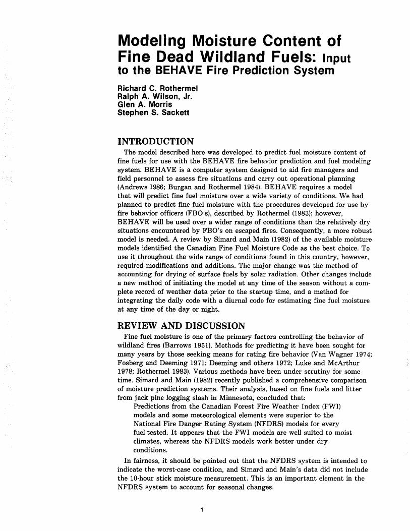
INTRODUCTION The model described here was developed to predict fuel moisture content of

fine fuels for use with the BEHAVE fire behavior prediction and fuel modeling system. BE HAVE is a computer system designed to aid fire managers and field personnel to assess fire situations and carry out operational planning (Andrews 1986; Burgan and Rothermel 1984). BEHAVE requires a model that will predict fine fuel moisture over a wide variety of conditions. We had planned to predict fine fuel moisture with the procedures developed for use by fire behavior officers (FBO's), described by Rothermel (1983); however, BEHAVE will be used over a wider range of conditions than the relatively dry situations encountered by FBO's on escaped fires. Consequently, a more robust model is needed. A review by Simard and Main (1982) of the available moisture models identified the Canadian Fine Fuel Moisture Code as the best choice. To use it. throughout the wide range of conditions found in this country, however, required modifications and additions. The major change was the method of accounting for drying of surface fuels by solar radiation. Other changes include a new method of initiating the model at any time of the season without a com­plete record of weather data prior to the startup time, and a method for integrating the daily code with a diurnal code for estimating fine fuel moisture at any time of the day or night.

REVIEW AND DISCUSSION Fine fuel moisture is one of the primary factors controlling the behavior of

wildland fires (Barrows 1951). Methods for predicting it have been sought for many years by those seeking means for rating fire behavior (Van Wagner 1974; Fosberg and Deeming 1971; Deeming and others 1972; Luke and McArthur 1978; Rothermel 1983). Various methods have been under scrutiny for some time. Simard and Main (1982) recently published a comprehensive comparison of moisture prediction systems. Their analysis, based on fine fuels and litter from jack pine logging slash in Minnesota, concluded that:

Predictions from the Canadian Forest Fire Weather Index (FWI) models and some meteorological elements were superior to the National Fire Danger Rating System (NFDRS) models for every fuel tested. It appears that the FWI models are well suited to moist climates, whereas the NFDRS models work better under dry conditions.

In fairness, it should be pointed out that the NFDRS system is intended to indicate the worst-case condition, and Simard and Main's data did not include the 10-hour stick moisture measurement. This is an important element in the NFDRS system to account for seasonal changes.

Because the FBO procedures (Rothermel 1983) are based in part on the NFDRS models, and because users of BEHAVE will not usually have 10-hour stick moisture data available, we decided to evaluate the Canadian Fine Fuel Moisture Code for use with BEHAVE.

The Fine Fuel Moisture Code (FFMC) is a component of the Canadian Forest Fire Weather Index System (Canadian Forestry Service 1984). The literature is rich with descriptors of the Canadian Fire Weather Index and the moisture codes. We will not attempt to summarize it all here. Van Wagner (197-4) describes the evolution of the index:

The FFMC was developed from concurrent weather and fuel moisture data obtained in pine stands at Petawawa, Ontario, by multiple corre­lation of present moisture content with current weather and previous day's moisture content. Although pine needles are relatively fast dry­ing, they found that there was a substantial effect of the previous day's moisture content which meant that drying cannot be assumed to be instantaneous. Thus, the method of estimating fuel moisture is based on a known or previous value and adjustment to it according to weather during the intervening 24 hours. The rate of change is commensurate with atmospheric conditions imposed upon the fuel and the final equilibrium value. This code calculates a daily value of fine fuel moisture for the afternoon.

The idea of yesterday's fuel moisture content affecting today's fine fuel mois­ture content may be hard to accept by those trained to equate fine fuels with I-hour time lags. However, recent information shows that some conifer needles have time lags as long as 30 hours (Anderson 1985). These fuels will not come close to equilibrium in a typical 24-hour diurnal cycle.

Because the FFMC was developed from data taken beneath a canopy of jack pine trees, it cannot adequately account for drying of fuels exposed to the sun; a condition important to the fuels in a large part of the world.

The effects of solar radiation on fuel moisture and fire hazard were recognized early in the present century (for example, Plumnler 1912). Gast and Stickel (1929) found that "diminution in the radiation intensity incident upon the duff reduces the rate at which the duff moisture content decreases during the day," and further suggested " ... the importance of a cloud 'weather eye' to patrol­men. By estimating cloudiness, the probable hazard can be estimated."

Gisborne (1928) gives data for exposures to different totals of radiation and concludes that determining changes in moisture is of value only when the amount of shielding from sunlight is varied. Gisbome (1933) hypothesized a mechanism of wind and solar radiation to account for observations of dead wood lying on the ground being drier than in air. Again, Gisborne (1936), explaining the operation of his forest fire danger meter, referenced the work of Hornby (1935) who also emphasized exposure to sun and wind in fuel classifica­tion. Byram (1940) reported that his experiment showed excellent evidence that the effects of wind and sunshine on fuel moisture are not additive, but partially compensating; that the energy of sunshine seems to be a very powerful drying agent, and wind prevents some of this energy from being absorbed by the fuels; and, further, that the reflection factor of fuels has considerable effect on their moisture content when exposed to sunlight-black sticks absorbing more than

2

white, hence having lower moisture contents. Countryman (1977) found mois­ture variation under a ponderosa pine stand (Pinus ponderosa Laws.) to have significant variation within short distances-enough to offset ignition and fire behavior significantly. These variations were found to be caused primarily by solar radiation reaching some litter areas through openings in the crown canopy and cooling directly under the openings at night. Catchpole and Catchpole (1983) found that a large portion of the variation in spread rate of experimental grass fires in Australia (statistical variation between fires) could be attributed to the degree of cloud cover.

In 1943 Byram and Jemison reported on a method they developed whereby radiation intensity could be determined for any season of year, hour of day, slope, and aspect. They established a relationship of solar radiation intensity to surface fuel moisture equilibria and rates of drying. Van Wagner (1969) used Byram and Jemison's model as a basis for investigating the effect of solar heating and wind on the surface temperature of jack pine needles and quaking aspen leaves. He obtained results similar to theirs with a slightly different mathematical form. The solar heating section of our model is an extension and application of Byram and Jemison's original idea.

In the interim many authors have investigated solar irradiance on the terres­trial surface (Kimball 1919; Bates and Henry 1928; Okanoue 1957; Lee 1962; Loewe 1962; Kaufmann and Weatherred 1982; Running and Hungerford 1983).

The correct solar;,terrestrial geometry varies among authors only in detail. Our customers will be oriented to local standard time; to measuring slope aspect clockwise from north; to measuring slope angle positive (up) in the sense opposite the slope aspect ... etc.

We wish also to circumvent the popular concept of "equivalent slope" because of the geometric difficulties encountered when the shade trees are standing at tilted slant angles on that "equivalent horizontal slope." (See, for example, Okanoue, Lee, Kaufmann and Weatherred.)

OBJECTIVES Our objectives in developing a new model are to predict the moisture of fine

dead fuels with greater accuracy over a wider range of conditions and times than possible with the FBO procedures (Rothermel 1983). The main concerns with the FBO system are its inability to account for precipitation prior to the day of the fire and its tendency in northern latitudes to underestimate moisture values of fuels beneath a forest canopy.

Simard and Main suggest at least five characteristics of a fuel and its environment that must be specified when developing a predictive model:

1. Composition of the material (wood, needles, leaves, grass).

2. Presence of surface layer (bark, wax).

3. Thickness (diameter of wood). 4. Location (on, off the ground).

5. Environment (under a canopy, in the open).

3

A summary of the characteristics to be accounted for by this model is given below:

1. The model will be applicable to fine dead fuels, needles, leaves, cured herbaceous plants, and dead stems less than one-fourth inch in diameter.

2. The model should be sensitive to atmospheric moisture. This is the most common factor in all models wherein an equilibrium fuel moisture is determined based on air temperature and humidity and the fuel moisture is continually seeking this equilibrium value. (The influence of soil moisture on fuel moisture, perhaps through dew formation, is an important consideration for future revisions to this model.)

3. The model should be sensitive to the drying effect of solar radiation. This requires a considerable amount of additional information. The amount of solar heating depends upon day length, sun angle, windspeed, and shade. These, in turn, depend upon time of year, latitude, slope, aspect, cloud cover, and overstory conditions.

4. The model should be sensitive to precipitation occurring within 7 days preceding the fire.

5. The model should be capable of predicting fuel moisture any time of the day or night.

6. The model should be capable of accounting for elevation differences by adjusting temperature and humidity to fire locations above or below the position where they are measured.

7. Inputs must be available to a knowledgeable person without requiring a previously assembled weather data file.

B. Because the fuel moisture is intended for use in a fire behavior model (Rothermel 1972; Albini 1976), wherein fires are in fuels with moistures less than a specified moisture of extinction (usually less than 30 percent), attention will be concentrated on accuracy at the lower levels.

9. The model should account for atmospheric haze.

Considerations omitted at this time are:

1. Differences in moisture because fuels are either standing (such as grass) or lying on the ground.

2. Differences between freshly fallen and old litter. 3. Differences caused by fuel coating, such as bark or wax. 4. The effect of dew. 5. The effect of moisture in the duff and soil beneath the litter layer.

The reasons for omitting these influences at this time are threefold: (1 ) We do not have the necessary information to model the process; (2) every new model requires data from the user when applying the model, and it is not clear how some of these data would be known to the user; and (3) a necessity to derive a solution in a reasonable time, with a strong expectation that the planned improvements will make the model significantly better than present methods.

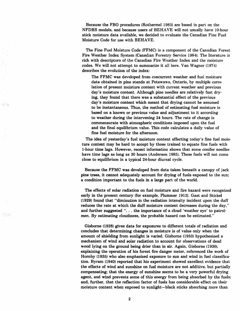
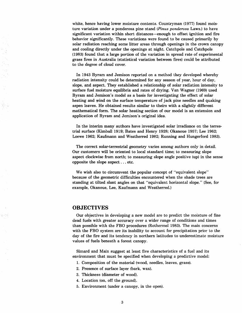
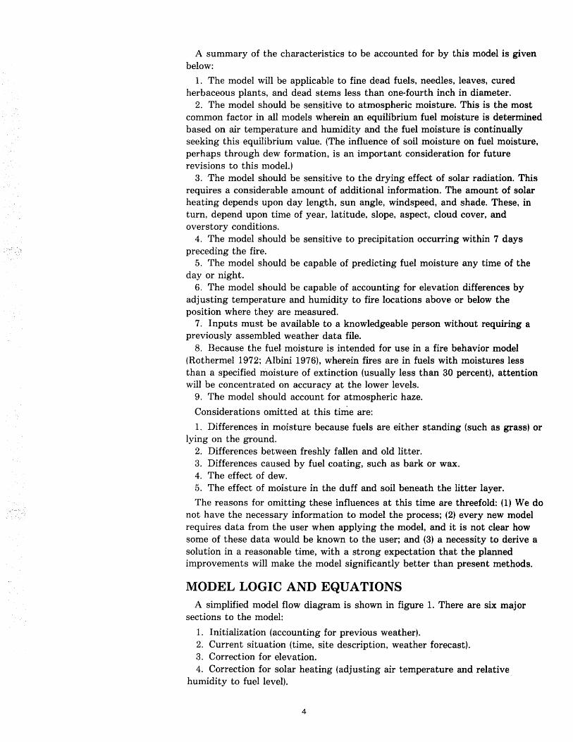
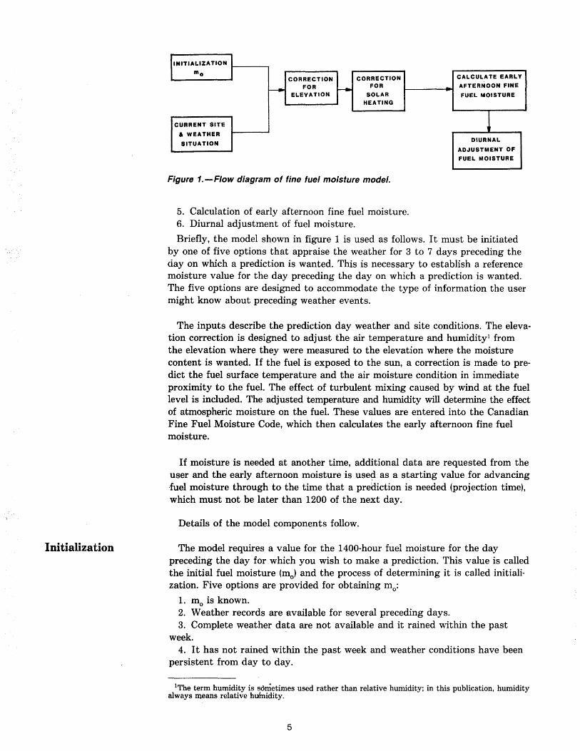
MODEL LOGIC AND EQUATIONS A simplified model flow diagram is shown in figure 1. There are six major

sections to the model:

1. Initialization (accounting for previous weather). 2. Current situation (time, site description, weather forecast). 3. Correction for elevation. . 4. Correction for solar heating (adjusting air temperature and relative

humidity to fuel level).

4

Initialization

INITIALIZATION

mo CORRECTION CALCULATE EARLY CORRECTION

f---I- FOR r--- FOR AFTERNOON FINE

ELEVATION SOLAR FUEL MOISTURE HEATING

CURRENT SITE ~ a WEATHER

SITUATION DIURNAL

ADJUSTMENT OF

FUEL MOISTURE

Figure 1.-Flow diagram of fine fuel moisture model.

5. Calculation of early afternoon fine fuel moisture. 6. Diurnal adjustment of fuel moisture.

Briefly, the model shown in figure 1 is used as follows. It must be initiated by one of five options that appraise the weather for 3 to 7 days preceding the day on which a prediction is wanted. This is necessary to establish a reference moisture value for the day preceding the day on which a prediction is wanted. The five options are designed to accommodate the type of information the user might know about preceding weather events.

The inputs describe the prediction day weather and site conditions. The eleva­tion correction is designed to adjust the air temperature and humidityl from the elevation where they were measured to the elevation where the moisture content is wanted. If the fuel is exposed to the sun, a correction is made to pre­dict the fuel surface temperature and the air moisture condition in immediate proximity to the fuel. The effect of turbulent mixing caused by wind at the fuel level is included. The adjusted temperature and humidity will determine the effect of atmospheric moisture on the fuel. These values are entered into the Canadian Fine Fuel Moisture Code, which then calculates the early afternoon fine fuel moisture.

If moisture is needed at another time, additional data are requested from the user and the early afternoon moisture is use~ as a starting value for advancing .fuel moisture through to the time that a prediction is needed (projection time), which must not be later than 1200 of the next day.

Details of the model components follow.

The model requires a value for the 1400-hour fuel moisture for the day preceding the day for which you wish to make a prediction. This value is called the initial fuel moisture (mo) and the process of determining it is called initiali­zation. Five options are provided for obtaining mo:

1. mo is known. 2. Weather records are available for several preceding days. 3. Complete weather data are not available and it rained within the past

week. 4. It has not rained within the past week and weather conditions have been

persistent from day to day.

l'rhe term humidity is sometimes used rather than relative humidity; in this publication, humidity always means relative huhUdity.

5

5. It has not rained within the past week and weather conditions have been variable.

These options do not exhaust all ways of initiating the model. As the user becomes familiar with the initialization process, it will be seen that these options can be adapted to needs and ~limates. For instance, option 3 may work very well even if there were no rain at the beginning of the period.

Option 1 - mC' is known.-If the previous day's early afternoon fine fuel mois­ture is known from measurement or a previous calculation or an estimate, it may be used directly. 2

Option 2 - weather records available.-If the standard NFDR early afternoon fire weather measurements are available for 3 to 7 preceding days, the follow­ing data are entered for early afternoon of each day:

air temperature

relative humidity

amount of rain

20-foot windspeed

percent cloud cover

The 1400-hour moisture for the first day of the series is obtained by iterating the first day's weather data with the sun-adjusted FFMC until an equilibrium solution is reached. Then the data from each subsequent day are used as per the normal procedures of the Canadian system. The final value of moisture cal­culated in this initialization process is used as mo. This tedious option can be avoided by most users. It is included for those who wish to be exact or test the system.

Option 3 - complete weather data not available, and rain occurred.- If it has rained within the past week and if there has been no frontal passage since it rained, this option may be used.

Rain can act as a triggering event, causing a major change in fine fuel mois­ture. The occurrence of rain is a logical choice for initiating a new moisture prediction. The occurrence of rain is also unique enough that a fire manager could be expected to know or be able to find out when the last rainfall occurred and be able to estimate how much. The assumption of no frontal passage is necessary to make calculations about the air mass between the time of rain and proj ection time.

Enter: (1) How many days since it rained (2 to 7).

(2) Amount of rain, inches.

(3) The early afternoon temperature on the day it rained. (4) What has been the sky condition on the days since it rained?

(a) clear

(b) cloudy

(c) partly cloudy.

2If the NFDR lO-hour stick moisture is known, Simard (personal communication) has shown that fine fuel moisture can be calculated from the formula m =-8.74 + 2.90 (IO-h). This correlation was made in the Lake States; it is not known how well it works elsewhere.

6

, "~: .

These will give cloud cover values of 10, 90, and 50 percent, respectively.

(5) Today's (fuel moisture projection day) complete weather data (measured or forecast).

On the day it rained, the model assumes humidity = 90 percent, cloud cover = 90 percent, and windspeed = 5 mi/h if these values are not known. Early after­noon temperature and humidity on the days since it rained are reconstructed as follows: temperature is adjusted linearly between the day it rained and today. Today's dewpoint is calculated from today's temperature and humidity. Using the assumption of constant air mass since it rained, the humidity on each day is calculated from today's dewpoint and the linearly estimated temperature for each day. (Se~ appendix F for humidity calculation from dew point.)

When fuel moisture on the day before it rained is unknown, it is set to equilibrium for conditions on the day it rained. Any error will be overcome by the rain and successive calculations.

Option 4 - no rain within the past week and weather persistent.-Under these conditions, the fine fuel moisture will also persist from day to day. Today's early afternoon weather is iterated to find an equilibrium value.

Option 5 - no data available and weather during the preceding week has been variable.-Here, none of the preceding four situations can be utilized, but an estimate can be made as follows:

(1) Estimate yesterday's early afternoon weather conditions.

(2) What was the general weather pattern before yesterday? (a) hot and dry

(b) cool ~d wet (c) between (a) and (b).

These will give initial fuel moisture values of 6, 76, and 16 percent respectively. These rough estimates will be adjusted twice, once by yesterday's estimated weather and once by today's measured or forecasted weather.

Elevation Correction It is often impossible or impractical to measure the weather at the site where the fuel moisture estimate is needed. In mountainous terrain, the temperature and moisture of the atmosphere change with elevation. For a well-mixed atmosphere, the adiabatic lapse rate is used to adjust temperature and humid­ity according to elevation differences. The correction amounts to 3.5 of per 1,000 feet for temperature and 101°F per 1,000 feet for the dewpoint. Both cor­rections decrease with elevation. This correction has lieen used by others deal­ing with mountain meteorology (Running and Hungerford 1983).

Solar Heating

The corrections should only be applied when there is good mixing, such as in the late morning and afternoon when inversions have broken, and at night if neither location lies within an inversion.

If elevation differences are small, say less than 1,000 feet, the correction is ignored.

Many fuels in the United States, particularly rangelands in the West and Southwest, are exposed to considerable solar heating. We wanted the moisture model for BEHAVE to be able to account for this, but not to underpredict

7

moisture, as the FBO model often does, in northern latitudes under a forest canopy.

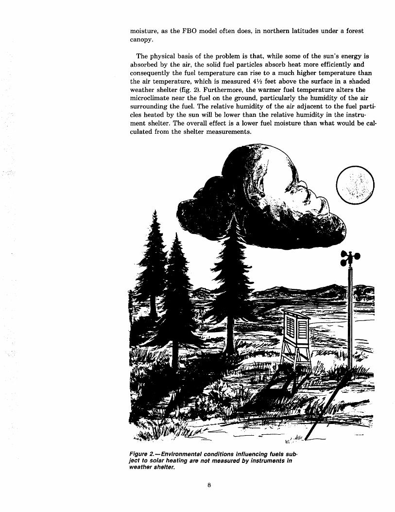
The physical basis of the problem is that, while some of the sun's energy is absorbed by the air, the solid fuel particles absorb heat more efficiently and consequently the fuel temperature can rise to a much higher temperature than the air temperature, which is measured 4Y2 feet above the surface in a shaded weather shelter (fig. 2). Furthermore, the warmer fuel temperature alters the microclimate near the fuel on the ground, particularly the humidity of the air surrounding the fuel. The relative humidity of the air adjacent to the fuel parti­cles heated by the sun will be lower than the relative humidity in the instru­ment shelter. The overall effect is a lower fuel moisture than what would be cal­culated from the shelter measurements.

Figure 2.-Environmental conditions influencing fuels sub· ject to solar heating are not measured by instruments in weather shelter.

8

Wind sweeping over the fuel confounds the problem. The moving air above the fuel will be cooler than the thin layer of air surrounding the fuel particles. Consequently, any turbulent mixing will tend to cool the air near the fuel, bringing it closer to the general air temperature and humidity.

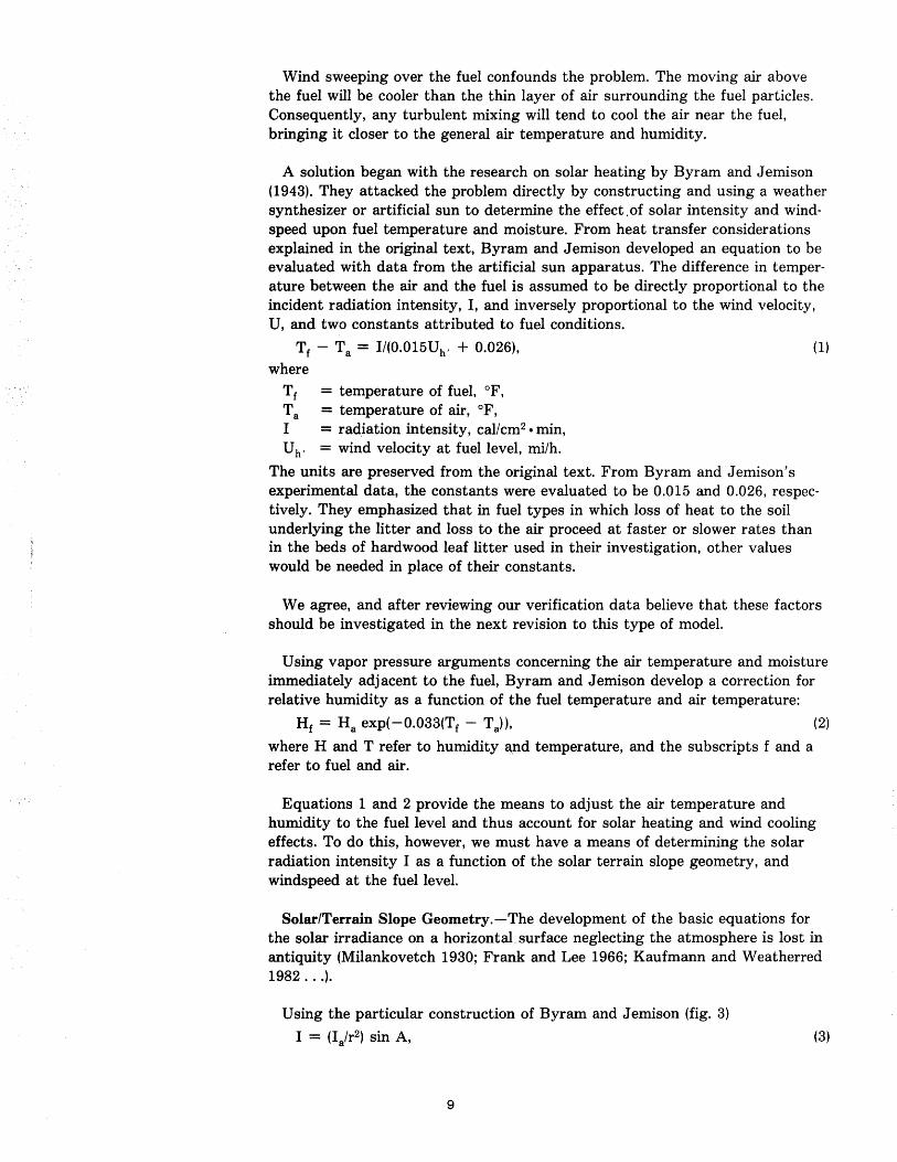
A solution began with the research on solar heating by Byram and Jemison (1943). They attacked the problem directly by constructing and using a weather synthesizer or artificial sun to determine the effect.of solar intensity and wind­speed upon fuel temperature and moisture. From heat transfer considerations explained in the original text, Byram and Jemison developed an equation to be evaluated with data from the artificial sun apparatus. The difference in temper­ature between the air and the fuel is assumed to be directly proportional to the incident radiation intensity, I, and inversely proportional to the wind velocity, U, and two constants attributed to fuel conditions.

T f - Ta = I1(0.015Uh , + 0.026), (1)

where

Tf

Ta I

= temperature of fuel, of, = temperature of air, of, = radiation intensity, cal/cm2 • min, = wind velocity at fuel level, mi/h.

The units are preserved from the original text. From Byram and Jemison's experimental data, the constants were evaluated to be 0.015 and 0.026, respec­tively. They emphasized that in fuel types in which loss of heat to the soil underlying the litter and loss to the air proceed at faster or slower rates than in the beds of hardwood leaf litter used in their investigation, other values would be needed in place of their constants.

We agree, and after reviewing our verification data believe that these factors should be investigated in the next revision to this type of model.

U sing vapor pressure arguments concerning the air temperature and moisture immediately adjacent to the fuel, Byram and Jemison develop a correction for relative humidity as a function of the fuel temperature and air temperature:

Hf = Ha exp(-0.033(Tf - Ta)), (2)

where H and T refer to humidity l:\l1d temperature, and the subscripts f and a refer to fuel and air.

Equations 1 and 2 provide the means to adjust the air temperature and humidity to the fuel level and thus account for solar heating and wind cooling effects. To do this, however, we must have a means of determining the solar radiation intensity I as a function of the solar terrain slope geometry, and windspeed at the fuel level.

Solar/Terrain Slope Geometry.-The development of the basic equations for the solar irradiance on a horizontal. surface neglecting the atmosphere is lost in antiquity (Milankovetch 1930; Frank and Lee 1966; Kaufmann and Weatherred 1982 ... ).

Using the particular construction of Byram and Jemison (fig. 3)

I = (la/r2) sin A,

9

(3)

.~ ., ..

z: l-i .... N

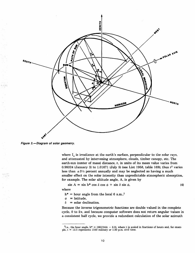
Figure 3. - Diagram of solar geometry.

where Ia is irradiance at the earth's surface, perpendicular to the solar rays, and attenuated by intervening atmosphere, clouds, timber canopy, etc. The earth-sun (center of mass) distance, r, in units of its mean value varies from 0.98324 (January 3) to 1.01671 (July 5) (see List 1958, table 169); thus r2 varies less than ± 3Y2 percent annually and may be neglected as having a much smaller effect on the solar intensity than unpredictable atmospheric absorption, for example. The solar altitude angle, A, is given by

sin A = sin h * cos a cos c/> + sin a sin C/>,

where h* = hour angle from the local 6 a.m.,3 c/> = latitude, a = solar declination.

(4)

Because the inverse trigonometric functions are double valued in the complete cycle, 0 to 271", and because computer software does not return angular values in a consistent half cycle, we provide a redundant calculation of the solar azimuth

3i.e., the hour angle, h* = (360/24)(t - 6.0), where t is scaled in fractions of hours and, for exam­ple, t = 13.5 represents 1330 military or 1:30 p.m. civil time.

10

to remove the double value ambiguity. (There is no ambiguity in the solar ele­vation angle, A, if it is understood that -7r/2 :s A :s 7r/2. There are situations, however, where the solar azimuth must range the full 27r circle.)

Thus, from figure 3,

tan. z = sin h* cos 0 sin cP - sin 0 cos cP , and cos h* cos 0

cos z = cos h* cos olcos A.

(5)

(6)

By simple ratios of equations 5 and 6, any function of solar azimuth, z, may be calculated over the full range 0 :s z :s 27r.

Kaufmann and Weatherred (1982) give the analytic solution to List's tabular values of r and 0:

r2 = 0.999847 + 0.001406 (0),

o = 23.5 sin(0.9863(284 + NJ ))

= solar declination in degrees, NJ = Julian date

= Integer Value (31(Mo - 1) + Dy - 0.4Mo - 1.8 + e)

12 if Mo = 1,

_ 3 if Mo= 2, ~ - 1 if Mo> 2 on leap years,

o otherwise.

(7)

(8)

Mo and Dy are the month and day, respectively, of the Gregorian calendar and Integer Value means round up or down to nearest integer.

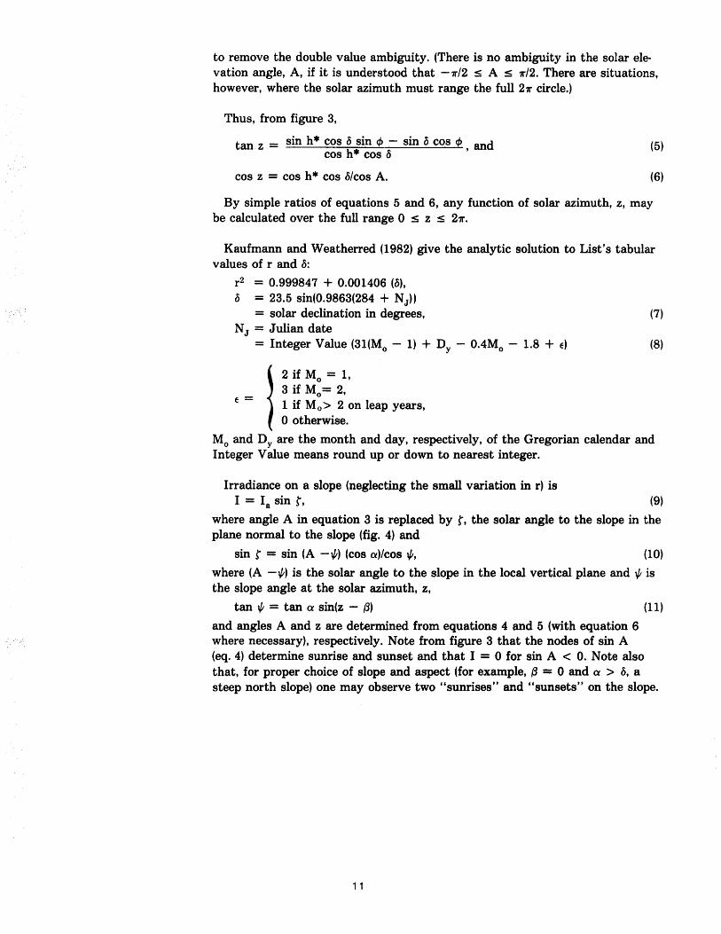
Irradiance on a slope (neglecting the small variation in r) is I = la sin t, (9)

where angle A in equation 3 is replaced by t, the solar angle to the slope in the plane normal to the slope (fig. 4) and

sin t = sin (A -1/;) (cos a)/cos 1/;, (10)

where (A -1/;) is the solar angle to the slope in the local vertical plane and 1/; is the slope angle at the solar azimuth, z,

tan 1/; = tan a sin(z - 13) (11)

and angles A and z are determined from equations 4 and 5 (with equation 6 where necessary), respectively. Note from figure 3 that the nodes of sin A (eq. 4) determine sunrise and sunset and that I = 0 for sin A < O. Note also that, for proper choice of slope and aspect (for example, (3 ::;: 0 and a > 0, a steep north slope) one may observe two "sunrises" and "sunsets" on the slope.

11

HORIZONTAL

Figure 4. - Diagram of sun/slope geometry.

Obscuration and Attenuation of Irradiance.-The irradiance, la' of equation 9, on the forest floor is the product of the incident solar power density and the transmittance of the intervening media:

la = IMTn' (12)

where Tn is the net transmittance of clouds and trees discussed below, and 1M is the direct solar irradiance including atmospheric attenuation.

The direct solar irradiance, 1M , may be written (see Kondratyev 1969, ch. 5, or Johnson 1960, ch. 4):

(13)

where 10 is the incident intensity or solar constant, 1.98 cal/cm2 -min (variously quoted as 10 = 1.84 to 1.98 cal/cm2-min).

p is the transparency coefficient (integral over all wavelengths). M, the optical air mass, is the ratio of the optical path length, lM' of radiation

through the atmosphere at angle, A, to the path length, lzo' toward the zenith from sea level. Thus

(14)

12

The air mass M is referenced to the optical path lzo at sea level. If one is working at a few thousand feet elevation, the zenith air mass optical path, lz' is significantly reduced (at 5 km elevation you are above half of the air mass!):

lz = lzo e l eo ' (15) where e is the absolute atmospheric pressure at the site and eo is the sea level pressure (1,000 mb). For an elevation, E, in feet above sea level, e is approximately

e = eo exp (-0.0000448E). Thus,

M = (el eo) csc A = exp( -0.0000448E) csc A, and (16)

Ia = Io7npM. (17)

Because of the earth's curvature, optical refraction by the air density gradient, etc., the exact csc A dependence of solar irradiance on solar altitude angle fails near the horizon, that is, for A < 10 degrees. But because the irradiation just after sunrise and before sunset is "small" and the probability of shading is very high, we will let the approximation stand for those small angles.

Atmospheric transparency, p, is most notably dependent on absorption of radiation by differing amounts of atmospheric moisture and by atmospheric turbidity (haze). Even an empirical estimation of p requires knowledge (radio­sonde measurement) of the vertical distribution of temperature, pressure, and relative humidity in addition to measures of dust-haze and particulates. Acqui­sition of such data is beyond the scope of the BEHAVE system. It is sufficient to say that Byram and Jemison used a constant p = 0.7, which they assumed was a "reasonable average for a thin layer of rather dense haze which is com­mon at 2,000 feet during the fire season in the southern Appalachians," and that a 30-year mean value at Pavlovsk, Russia (Kondratyev 1969) was p = 0.745, with extreme values of 0.710 (1914) and 0.770 (1909) and a typical annual (12-month) variation of Ap = ±0.02 (except for the 2-year period following the eruption of Katmai volcano (Alaska) in 1912 when the annual average trans­parency was 0.57). Similar data are presented in the other monographs on atmospheric transparency. The mean Kondratyev value represents a "clean for­est atmosphe~e." On exceptionally clear days p may range as large as 0.8 and on very hazy days as small as 0.6, excluding direct interference from local smoke palls. The list below suggests a series of p values with qualitative descriptors for application by field observers.

P 0.8

Qualitative description

exceptionally clear atmosphere

0.75 average clear forest atmosphere 0.7 moderate forest (blue) haze

0.6 dense haze

13

Shade The net cloud/tree transmittance from above is

(18)

where Tt is the transmittance of the timber canopy and Tc = (1 - Si100) is the transmittance of cloud cover. Sc is scaled in percent.

Cloud Shade.-Cloud shade is familiar to users of the National Fire-Danger Rating System as a contribution to the state of the weather code. For this model the user can enter any percentage of cloud cover between 0 and 100. When working with the NFDRS state of weather code, convert to percent cloud cover according to the following:

NFDRS Shade code range Input

Pet Pet

0 o - 10 5 1 10 - 50 30 2 50 - 90 70 3 90 - 100 95

Tree Shade.-Many authors have suggested that the Beer-Lambert exponen­tial absorption model of solar radiation is applicable to forest plant communi­ties and that the Leaf Area Index (LAI) may be the significant attenuation parameter (Monsi and Saeki 1953; Jordan 1969; Barbour and others 1980).

Considerable work has been done to relate site productivity, habitat classifi­cation, and topographic distributions to LAI (see also Stage 1976; Pfister and others 1977; Zavitkovski 1976; Salomon and others 1976). Those relationships have not been satisfactorily established nor has LAI become a universally established mensurational parameter, so that we can use it in the present appli­cation. Instead, our site-specific approach to shade is an extension of the method suggested by Satterlund (1983). In the Satterlund approach the shadow area of an average tree on a unit surface area is calculated, then the fractional area of shadow cast by n trees is estimated. Because the tree crowns are not totally opaque we assume a Beer law attenuation and estimate the optical attenuation coefficient on the basis of shade tolerance and crown shape.

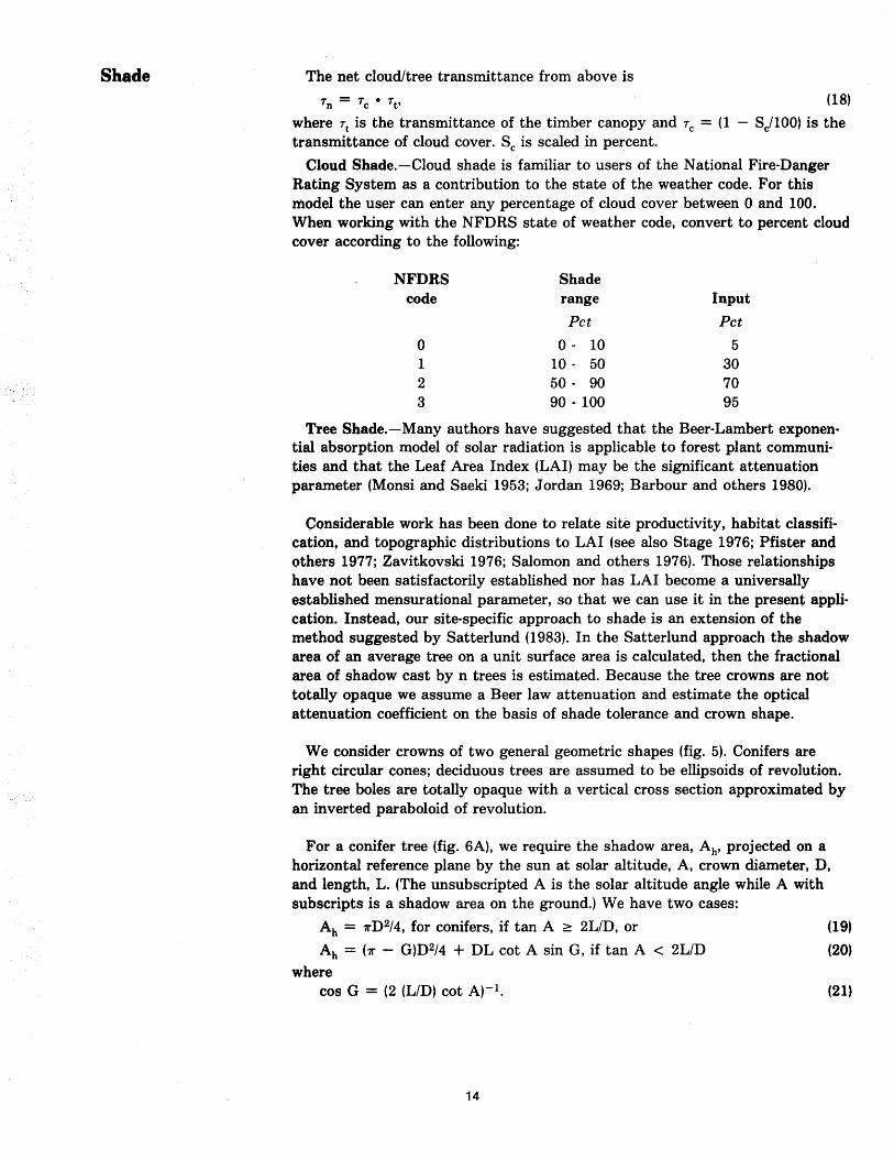
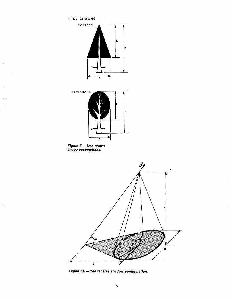
We consider crowns of two general geometric shapes (fig. 5). Conifers are right circular cones; deciduous trees are assumed to be ellipsoids of revolution. The tree boles are totally opaque with a vertical cross section approximated by an inverted paraboloid of revolution.

For a conifer tree (fig. 6A), we require the shadow area, Ah, projected on a horizontal reference plane by the sun at solar altitude, A, crown diameter, D, and length, L. (The unsubscripted A is the solar altitude angle while A with subscripts is a shadow area on the ground.) We have two cases:

Ah = 7I"D2/4, for conifers, if tan A ;::: 2L/D, or (19)

Ah = (71" - G)D2/4 + DL cot A sin G, if tan A < 2L/D (20)

where cos G = (2 (L/D) cot A)-I. (21)

14

TREE CROWNS

Fig~re 5;-Tree crown shape assumptions.

h

Figure 6A. -Conifer tree shadow configuration.

15

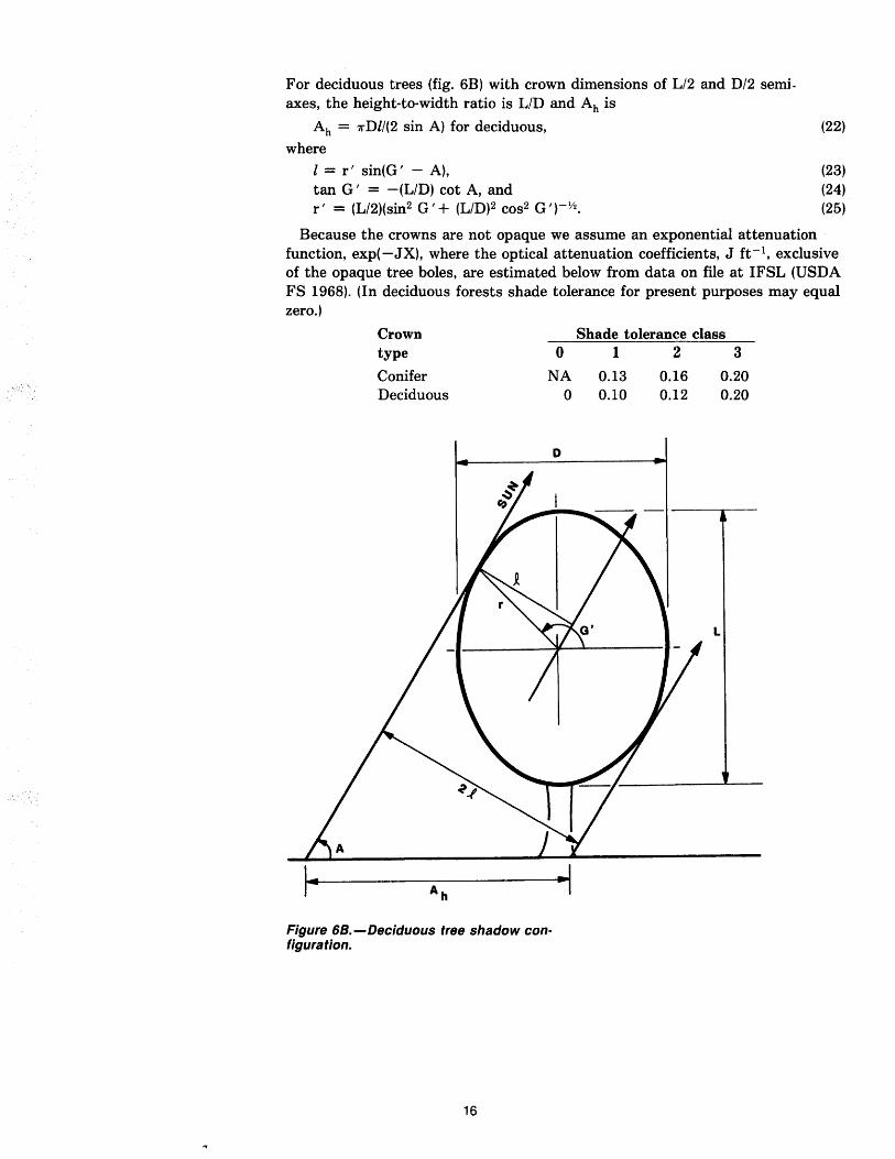
For deciduous trees (fig. 6B) with crown dimensions of L/2 and D/2 semi. axes, the height-to-width ratio is LID and Ah is

Ah = 7rDl/(2 sin A) for deciduous,

where

I = r' sin(G' - A), tan G' = -(LID) cot A, and r' = (L/2)(sin2 G'+ (L/D)2 cos2 G')-Y2.

(22)

(23) (24) (25)

Because the crowns are not opaque we assume an exponential attenuation function, exp(-JX), where the optical attenuation coefficients, J ft- 1, exclusive of the opaque tree boles, are estimated below from data on file at IFSL (USDA FS 1968). (In deciduous forests shade tolerance for present purposes may equal zero.)

Shade tolerance class Crown type o 1 2 3

Conifer Deciduous

NA o

D

Figure 6S.-Deciduous tree shadow con· figuration.

16

0.13 0.10

0.16 0.12

L

0.20 0.20

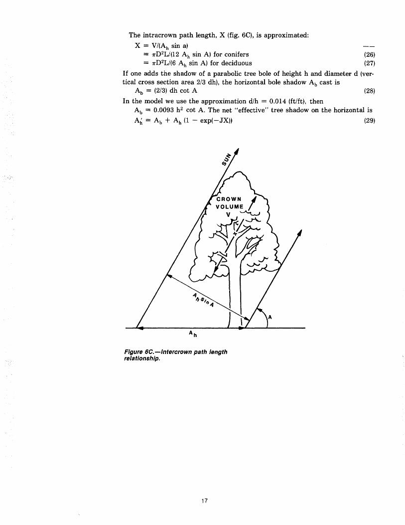
The intracrown path length, X (fig. 6e), is approximated:

X = V/(Ah sin a) = 7r D2LI (12 Ah sin A) for conifers = 7rD2L/(6 Ah sin A) for deciduous

(26)

(27)

If one adds the shadow of a parabolic tree bole of height h and diameter d (ver­tical cross section area 2/3 dh), the horizontal bole shadow Ab cast is

Ab = (2/3) dh cot A (28)

In the model we use the approximation dlh = 0.014 (ft/ft) , then Ab = O.Od93 h2 cot A. The net "effective" tree shadow on the horizontal is

Ah = Ab + Ah (1 - exp(-JX)) (29)

Figure Be. -In tercro wn path length relationship.

17

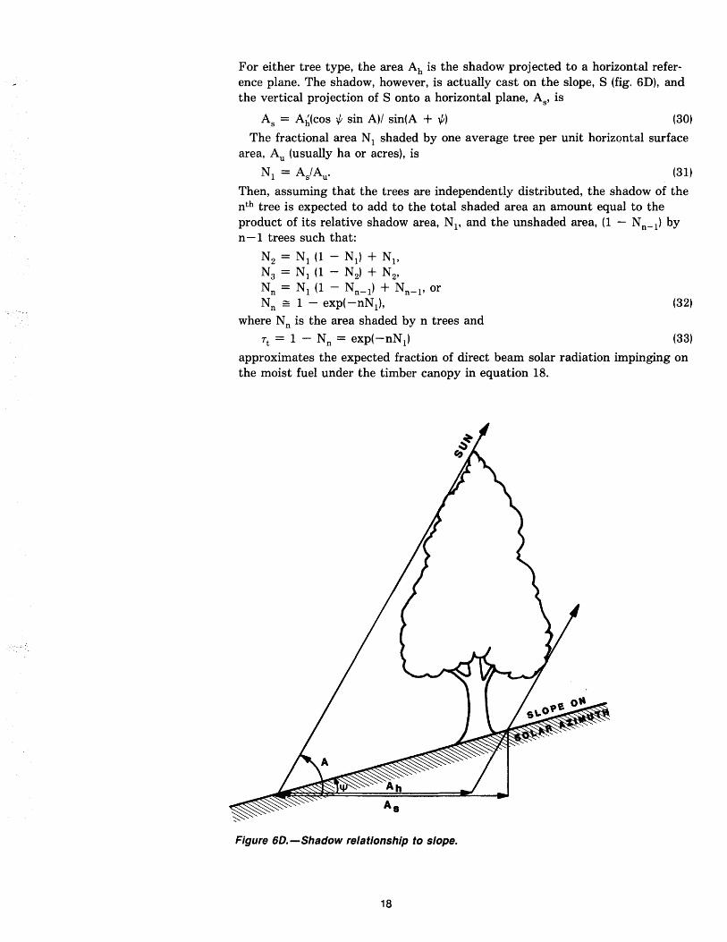
For either tree type, the area Ah is the shadow projected to a horizontal refer­ence plane. The shadow, however, is actually cast on the slope, S (fig. 6D), and the vertical projection of S onto a horizontal plane, As' is

As = Ah(cos 'I/; sin A)/ sin(A + '1/;) (30)

The fractional area N 1 shaded by one average tree per unit horizontal surface area, Au (usually ha or acres), is

Nl = As/Au' (31)

Then, assuming that the trees are independently distributed, the shadow of the nth tree is expected to add to the total shaded area an amount equal to the product of its relative shadow area, Nl' and the unshaded area, (1 - Nn- 1) by n -1 trees such that:

N2 = Nl (1 - N1) + NIt N 3 = N 1 (1 - N 2) + N 2' Nn = Nl (1 - Nn- 1) + Nn-l' or Nn == 1 - exp(-nN1),

where N n is the area shaded by n trees and Tt = 1 - Nn = exp(-nN1)

(32)

(33)

approximates the expected fraction of direct beam solar radiation impinging on the moist fuel under the timber canopy in equation 18.

Figure 6D.-Shadow relationship to slope.

18

Fuel Level Windspeed

An alternative estimate of the number of trees per unit area, n, that is con­sistent with this rationale is as follows: Given the crown closure, C, and aver­age tree diameter, D, then the vertically projected crown area, A;. of one tree is

A; = 7rD2/4 N{ = A~/Au'

By definition, then

N; = C = 1 - exp(-nN{) (34) n = -In(l - C)/N{ n = -4Au In(l - C)/7rD2 (35)

One must caution that A~ is not the proper effective crown area, As' used in equation 31. A; is the total area within the crown perimeter while calculations of As (in eq. 31) must include the transparency of the particular crown type as developed above.

A list of the equations and pertinent constants is given at the end of the text.

Byram and Jemison's equation for calculation of surface fuel temperature (eq. 1) requires a value for the windspeed at the fuel surface. This is not a trivial correction; even though wind speeds close to the surface are low, Byram and Jemison's data show that the cooling effect can be pronounced.

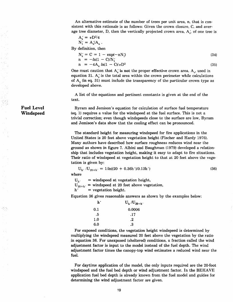
The standard height for measuring windspeed for fire applications in the United States is 20 feet above vegetation height (Fischer and Hardy 1976). Many authors have described how surface roughness reduces wind near the ground as shown in figure 7. Albini and Baughman (1979) developed a relation­ship that includes vegetation height, making it easy to adapt to fire situations. Their ratio of windspeed at vegetation height to that at 20 feet above the vege­tation is given by:

Uh , IU20+h , = 1Iln((20 + 0.36h ')/0.13h ') (36)

where

Uh , = windspeed at vegetation height, U20+h , = windspeed at 20 feet above vegetation, h' = vegetation height.

Equation 36 gives reasonable answers as shown by the examples below:

h' U h ,/U20+h '

0.1 .5

1.0 6.0

0.0006 .17 .2 .3

For exposed conditions, the vegetation height windspeed is determined by multiplying the windspeed measured 20 feet above the vegetation by the ratio in equation 36. For unexposed (sheltered) conditions, a fraction called the wind adjustment factor is input to the model instead of the fuel depth. The wind adjustment factor times the canopy-top wind estimates a reduced wind near the fuel.

For daytime application of the model, the only inputs required are the 20-foot windspeed and the fuel bed depth or wind adjustment factor. In the BEHAVE application fuel bed depth is already known from the fuel model and guides for determining the wind adjustment factor are given.

19

20 FT WIND

MID-FLAME

Figure 7.-Near·surface wind profile.

For nighttime application in uneven terrain, downslope winds may need to be considered. Slope winds do not follow the log reduction pattern used in day­time. At night, if the slope is less than 5 percent, use the daylight procedures. If the slope is greater than 5 percent, and if the 20-foot windspeed is less than 10 mi/h, let the vegetation height wind equal 4 mi/h (a reasonable assumption for downslope winds). If the windspeed is greater than 10 mi/h, consider the canopy closure; if the closure is less than 10 percent, use the daylight proce­dures. If the canopy closure is greater than 10 percent, assume the 20-foot winds are blocked and let the vegetation height wind equal 4 mi/h.

The effect of wind on fine fuel moisture is also incorporated directly in the Canadian Fine Fuel Moisture Code. Van Wagner (1974) explains that wind affects the log drying rate, k,

k = a + b (U20)0.5 (37)

where U 20 is the windspeed at 20 feet.

Consequently, windspeed in the Canadian code is directly related to the rate at which fuel moisture approaches equilibrium.

The two wind corrections (eqs. 36 and 37) use windspeed measured at differ­ent heights. The fine fuel moisture code was calibrated to winds measured at the international standard height, 10 meters, in the open. The solar heating cor­rection requires windspeed at the vegetation height. The U.S. standard estab­lished for NFDR stations is 20 feet. The ratio of windspeed at 10 m to 20 feet (6.1 m) can be calculated from equation 36 if the vegetation height is known. We assume the windspeed at 20 feet and 10 meters are the same in this model.

20

Canadian Standard Daily Fine Fuel Moisture Code (FFMC)

Canadian Hourly Fine Fuel Moisture Code

Diurnal Predictions

The FFMC accepts initial fuel moisture, temperature, humidity, wind, and rain as inputs. In our model, the FFMC is used to calculate fine fuel moisture after the inputs are adjusted for elevation and solar heating. The version used in our model is the same as used by Simard and Main (1982). Like any large system, the FFMC has undergone many revisions. Work on the FFMC subse­quent to the version we used is designed to provide consistency for table presentation and to give better moisture predictions' under very wet conditions, 100 to 250 percent. It is not expected that these changes would affect our model significantly. The formulations of the FFMC we used are given in appendix A.

The other major condition to be accounted for by this model is the capability to make a calculation of expected moisture content at any time of the day or night. As presently used, the Canadian standard daily FFMC is structured to give a moisture value for midafternoon with data collected at noon, local stan­dard time. Fortunately, the Canadian Forestry Service has also investigated diurnal prediction. Muraro and others (1969) used litter data sampled from a dry lodgepole pine site near Prince George, BC, to produce tables for adjusting the FFMC for various times of the day or night. Van Wagner (1972) developed a new scale supplemented with data from a jack pine forest at Petawawa, and produced a single table for predicting FFMC based on time, initial FFMC, and relative humidity.

Van Wagner (1977) developed a set of equations, similar to the standard daily FFMC, that would accept hourly weather data, thereby freeing the model from the restraint of the original data and a single value of humidity. Alexander and others (1984) programmed the equations so that hourly computations of the FFMC and other components of the Canadian Forest Fire Weather Index system could be made on a handheld calculator with weather measured or fore­cast hourly. The BEHAVE model, as will be shown, adds the capability of predicting the necessary weather elements over a 24-hour period.

Unfortunately, weather forecasts on an hourly basis for extended periods are not readily available. It was necessary, therefore, to devise a way of estimating hourly weather frem a few forecasts at key times. This is done by initiating the diurnal predictions from the daily moisture prediction and weather data at 1400 hours. This is supplemented with a forecast at the time when the prediction is needed and with estimates of weather data at sunset and sunrise if projection time is after sunset or sunrise. Temperature and relative humidity values at each hour are predicted from sinusoidal curves linking the 1400 weather to the projection time weather. No trend for wind or cloud cover can be justified, so linear interpolations are used. The model will not apply to days with precipita­tion after 1200 (noon). The model determines hourly values of the weather data needed and performs the adjustments for solar heating. If the user does not have a weather forecast, he/she can estimate the temperature at any of the key points and if the air mass :Q.as not changed, the model will estimate the humid­ity. This will be based on the dew point of the air at the last known condition (calculation shown in appendix).

Beyond noon, the process will begin with a new 1400 fuel moisture calculated by the daily code. A discontinuity in a smooth-line moisture trend can occur between late morning predictions made by the morning code and early after­noon predictions made by the daily code.

21

Curves used to match weather conditions during each period of the day are described below.

Early afternoon.-If the moisture is needed between 1200 and 1600, the daily value is sufficient and no adjustments are necessary. Personal discussions with Van Wagner confirm this view.

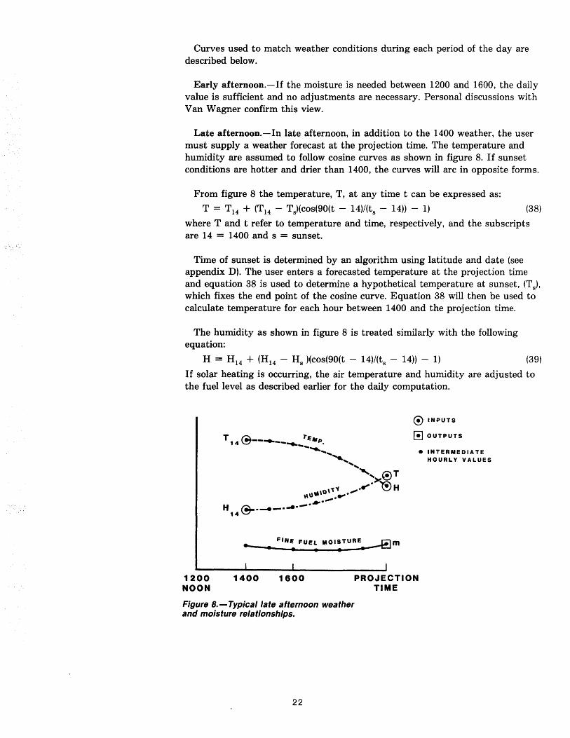
Late afternoon.-In late afternoon, in addition to the 1400 weather, the user must supply a weather forecast at the projection time. The temperature and humidity are assumed to follow cosine curves as shown in figure 8. If sunset conditions are hotter and drier than 1400, the curves will arc in opposite forms.

From figure 8 the temperature, T, at any time t can be expressed as:

T = T14 + (T14 - Ts)(cos(90(t - 14)/(ts - 14)) - 1) (38)

where T and t refer to temperature and time, respectively, and the subscripts are 14 = 1400 and s = sunset.

Time of sunset is determined by an algorithm using latitude and date (see appendix D). The user enters a forecasted temperature at the projection time and equation 38 is used to determine a hypothetical temperature at sunset, (T s),

which fixes the end point of the cosine curve. Equation 38 will then be used to calculate temperature for each hour between 1400 and the proj ection time.

The humidity as shown in figure 8 is treated similarly with the following equation:

H = H14 + (H14 - Hs )(cos(90(t - 14)/(ts - 14)) - 1) (39)

If solar heating is occurring, the air temperature and humidity are adjusted to the fuel level as described earlier for the daily computation.

T ~ t/!a. 1 4 ~--.... --..... "'''. --...... ,

''e. '"

" @T .. >""'Jr.:\ ort " " .. fI' \!I H ",uta' ........ ..,. . ...-

H _.

~.---- ..... 14 '=T"

... FIN/! FUEL MOISTURE ---i!lm . ..'

@ INPUTS

[!] OUTPUTS

• INTERMEDIATE HOURLY VALUES

1200 NOON

1400 1800 PROJECTION TIME

Figure 8. - Typical late afternoon weather and moisture relationships.

22

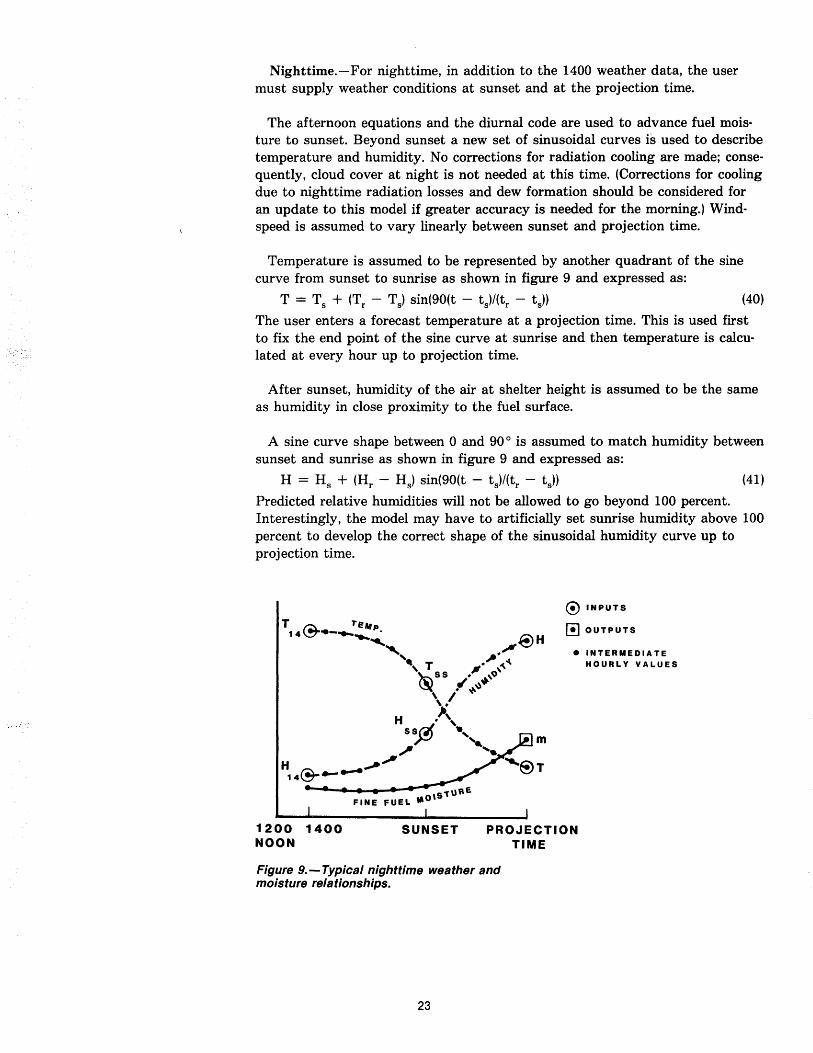
Nighttime.-For nighttime, in addition to the 1400 weather data, the user must supply weather conditions at sunset and at the projection time.

The afternoon equations and the diurnal code are used to advance fuel mois­ture to sunset. Beyond sunset a new set of sinusoidal curves is used to describe temperature and humidity. No corrections for radiation cooling are made; conse­quently, cloud cover at night is not needed at this time. (Corrections for cooling due to nighttime radiation losses and dew formation should be considered for an update to this model if greater accuracy is needed for the morning.) Wind­speed is assumed to vary linearly between sunset and projection time.

Temperature is assumed to be represented by another quadrant of the sine curve from sunset to sunrise as shown in figure 9 and expressed as:

T = Ts + (Tr - Ts) sin(90(t - ts)/(tr - t s)) (40)

The user enters a forecast temperature at a projection time. This is used first to fix the end point of the sine curve at sunrise and then temperature is calcu­lated at every hour up to projection time.

After sunset, humidity of the air at shelter height is assumed to be the same as humidity in close proximity to the fuel surface.

A sine curve shape between 0 and 90 0 is assumed to match humidity between sunset and sunrise as shown in figure 9 and expressed as:

H = Hs + (Hr - Hs) sin(90(t - ts)/(tr - t s)) (41)

Predicted relative humidities will not be allowed to go beyond 100 percent. Interestingly, the model may have to artificially set sunrise humidity above 100 percent to develop the correct shape of the sinusoidal humidity curve up to proj ection time.

1200 1400 NOON

SUNSET PROJECTION TIME

Figure 9. - Typical nighttime weather and moisture relationships.

23

Purpose of Validation

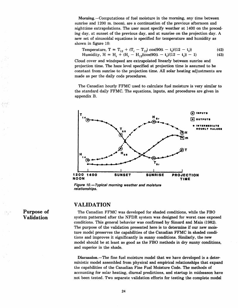
Morning.-Computations of fuel moisture in the morning, any time between sunrise and 1200 m. (noon), are a continuation of the previous afternoon and nighttime extrapolations. The user must specify weather at 1400 on the preced­ing day, at sunset of the previous day, and at sunrise on the projection day. A new set of sinusoidal equations is specified for temperature and humidity as shown in figure 10:

Temperature, T = T12 + (Tr - T12) cos(90(t - t r)/(12 - tr)) (42) Humidity, H = Hr + (Hr - H12)(cos(90(t - t r)/(12 - t r)) - 1) (43)

Cloud cover and windspeed are extrapolated linearly between sunrise and projection time. The haze level specified at projection time is assumed to be constant from sunrise to the projection time. All solar heating adjustments are made as per the daily code procedures.

The Canadian hourly FFMC used to calculate fuel moisture is very similar to the standard daily FFMC. The equations, inputs, and procedures are given in appendix B.

T ® INPUT.

14~ H .r r;t OUTPUT. \:]............... _ ~ L::J ........... .~.-..

.. ......... • INTIRIlIDIATI ~'- .'" ..... , T '" .... HOURLY VA LUI.

'~. / ~H ~ /. '( m . ,

I> '-', (t)T H ,II H.. "",."M"

1 4 ". ~ ..... .L.:L .......... @ .... .-. '-="'"

1200 1400 NOON

SUNSET

T. r

SUNRISE

Figure to.-·Typlcal morning weather and moisture relationships.

VALIDATION

PROJECTION TIME

The Canadian FFMC was developed for shaded conditions, while the FBO system patterned after the NFDR system was designed for worst case exposed conditions. This general behavior was confirmed by Simard and Main (1982). The purpose of the validation presented here is to determine if our new mois­ture model preserves the capabilities of the Canadian FFMC in shaded condi­tions and improves it significantly in sunny conditions. Similarly, the new model should be at least as good as the FBO methods in dry sunny conditions, and superior in the shade.

Discussion. - The fine fuel moisture model that we have developed is a deter­ministic model assembled from physical and empirical relationships that expand the capabilities of the Canadian Fine Fuel Moisture Code. The methods of accounting for solar heating, diurnal predictions, and startup in mid season have not been tested. Two separate validation efforts for testing the complete model

24

Daily Version Validation (Objective No.1)

were initiated. The first, reported here, uses data already available from several diverse fuel and shade conditions. The second is a study by the University of Montana to test the model independently. Their test will include a sensitivity analysis.

We were fortunate to find a great deal of moisture data with most of the inputs necessary to drive the model. Most of the data were unpublished. We used data from Idaho, Texas, Alaska, and Arizona. The Idaho data were col­lected at four elevations in conifer litter in the Bitterroot Mountains of Idaho, just south of Missoula (Frandsen and Bradshaw 1980). The Texas data were taken in grass fuels (Clark 1981). The Alaska data were taken in several fuel types and offer a good test of the model at northern latitudes (Norum 1983). Arizona data were taken in open and closed ponderosa pine stands (Harrington 1983; Sackett 1983, 1984). Sackett's data were the only set initiated after model development had been started so that all inputs were specified except haze. Data used in this analysis are shown in appendix G. Input data are in part A; outputs from the models are in part B.

Specific Objectives.-1. Determine if the daily version of the model can predict fine fuel moisture

better than the Canadian Fine Fuel Moisture Code when the fuels are exposed to the sun, and better than the FBO procedures when fuels are heavily shaded.

2. Determine if the initiation procedures that do not use a complete record of preceding weather work as well as those that do.

3. Determine how well the diurnal version of the model can predict fine fuel moisture throughout the diurnal cycle.

Analysis method. - When comparing predictions of models using the same data set, one of two models would probably be superior if it tends to have smaller errors than the other model. Two methods were used to compare the error distributions of the models:

1. Confidence intervals 2. Analysis of variance

The models are unaided by a posteriori correction terms or factors.

The confidence intervals consisted of the following (one unit is 1 percent of qvendry weight, the unit of fuel moisture):

PI = percent of predictions falling within 1 unit of the actual fuel moisture

P 3 = percent of predictions falling within 3 units of the actual value 190 = width of a 90 percent confidence interval about the actual value

The best model will have the largest values for PI and P 3 and the smallest 190,

Analysis of variance provides a basis for comparing model biases. The procedure gives a significance level (PF), which gauges the overall repeatability of different subsample means and the relative importance of these means for explaining overall variance. It can be determined if the sample mean error (x) of one model is significantly different from that of another by observing the contrast P-Ievels produced by the analysis of variance procedure. The data appear to satisfy the premises of analysis of variance reasonably well. Specifically, the contrast P-Ievels should be meaningful for comparing the BEHAVE and FFMC models in this analysis. The same is true for comparing the BEHAVE and FBO models except for the two hardwood strata, where the variances are no longer equal.

25

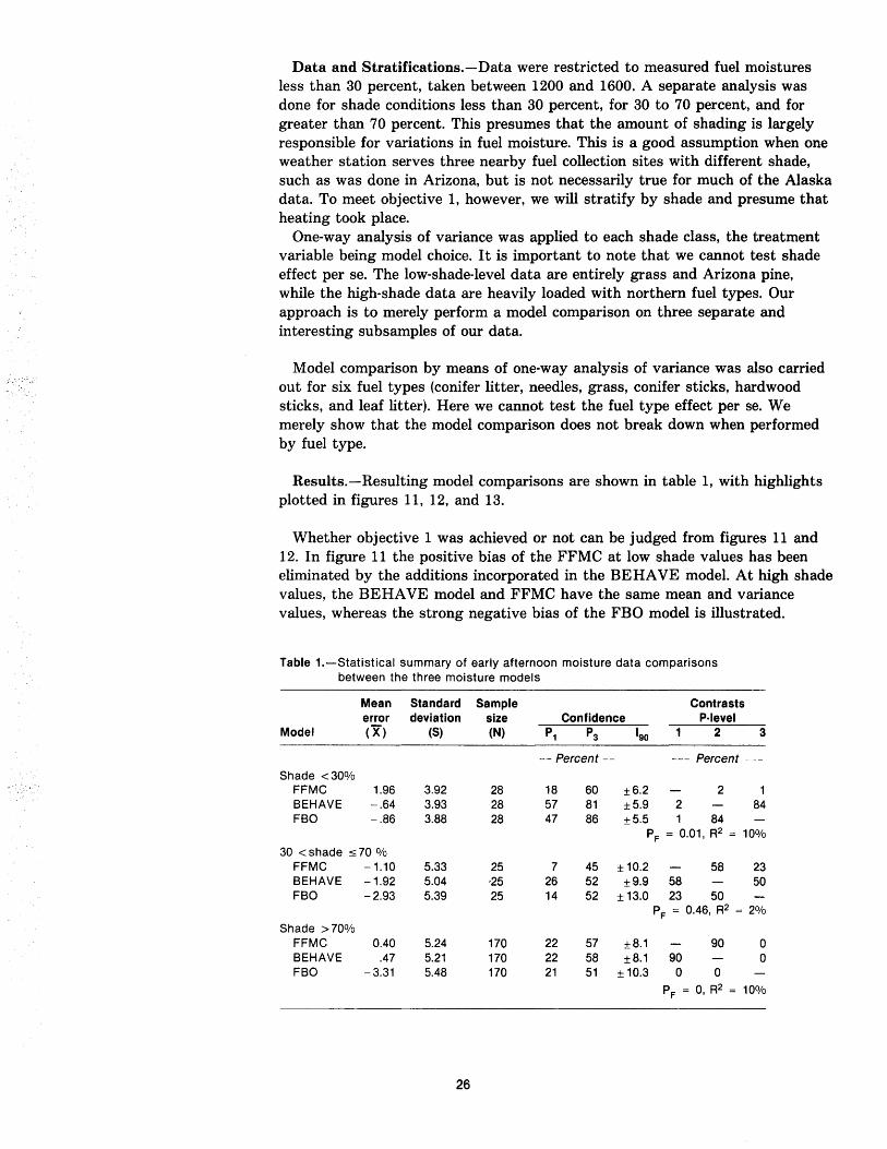
Data and Stratifications.-Data were restricted to measured fuel moistures less than 30 percent, taken between 1200 and 1600. A separate analysis was done for shade conditions less than 30 percent, for 30 to 70 percent, and for greater than 70 percent. This presumes that the amount of shading is largely responsible for variations in fuel moisture. This is a good assumption when one weather station serves three nearby fuel collection sites with different shade, such as was done in Arizona, but is not necessarily true for much of the Alaska data. To meet objective 1, however, we will stratify by shade and presume that heating took place.

One-way analysis of variance was applied to each shade class, the treatment variable being model choice. It is important to note that we cannot test shade effect per se. The low-shade-Ievel data are entirely grass and Arizona pine, while the high-shade data are heavily loaded with northern fuel types. Our approach is to merely perform a model comparison on three separate and interesting subsamples of our data.

Model comparison by means of one-way analysis of variance was also carried out for six fuel types (conifer litter, needles, grass, conifer sticks, hardwood sticks, and leaf litter). Here we cannot test the fuel type effect per se. We merely show that the model comparison does not break down when performed by fuel type.

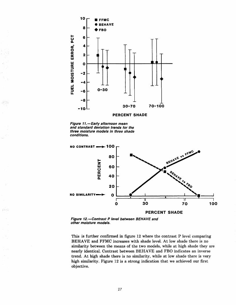
Results.-Resulting model comparisons are shown in table 1, with highlights plotted in figures 11, 12, and 13.

Whether objective 1 was achieved or not can be judged from figures 11 and 12. In figure 11 the positive bias of the FFMC at low shade values has been eliminated by the additions incorporated in the BEHAVE model. At high shade values, the BEHAVE model and FFMC have the same mean and variance values, whereas the strong negative bias of the FBO model is illustrated.

Table 1.-Statistical summary of early afternoon moisture data comparisons between the three moisture models

Mean Standard Sample Contrasts error deviation size Confidence P·level

Model (X) (S) (N) P1 P3 IgO 2 3

-- Percent -- --- Percent ---

Shade <30% FFMC 1.96 3.92 28 18 60 ±6.2 2 1 BEHAVE -.64 3.93 28 57 81 ±5.9 2 84 FBO -.86 3.88 28 47 86 ±5.5 1 84

PF = 0.01, R2 = 10%

30 <shade ~70 % FFMC -1.10 5.33 25 7 45 ±10.2 58 23 BEHAVE -1.92 5.04 -25 26 52 ±9.9 58 50 FBO -2.93 5.39 25 14 52 ± 13.0 23 50

PF = 0.46, R2 = 2%

Shade >70% FFMC 0.40 5.24 170 22 57 ±8.1 90 0 BEHAVE .47 5.21 170 22 58 ±8.1 90 0 FBO -3.31 5.48 170 21 51 ± 10.3 0 0

PF = 0, R2 = 10%

26

10 • FFMC • BEHAVE

8 +FBO

.... 6 0 a.

r£ 4 0 a: 2 a: LLI

LLI 0 a: ;:) ....

-2 0 0 :& -4 ... LLI ;:) -6 La.

-8

-to 30-70 70-100

PERCENT SHADE

Figure 11.-Early afternoon mean and standard deviation trends for the three moisture models in three shade conditions.

NO CONTRAST ~ 1 00

80 .... , " ....

Z w 60 0 rc w 40 Q.

20

NO SIMILARITY~ 0 I 0

"

II 30

ff~C ~ ..as

,,~~ ~~

" ~ • .,~~ '~41'. ,~ .. ',"I:-,~o

" " II

70

PERCENT SHADE

Figure 12.-Contrast P level between BEHAVE and other moisture models.

•

• . I 100

This is further confirmed in figure 12 where the contrast P level comparing BEHAVE and FFMC increases with shade level. At low shade there is no similarity between the means of the two models, while at high shade they are nearly identical. Contrast between BEHAVE and FBO indicates an inverse trend. At high shade there is no similarity, while at low shade there is very high similarity. Figure 12 is a strong indication that we achieved our first objective.

27

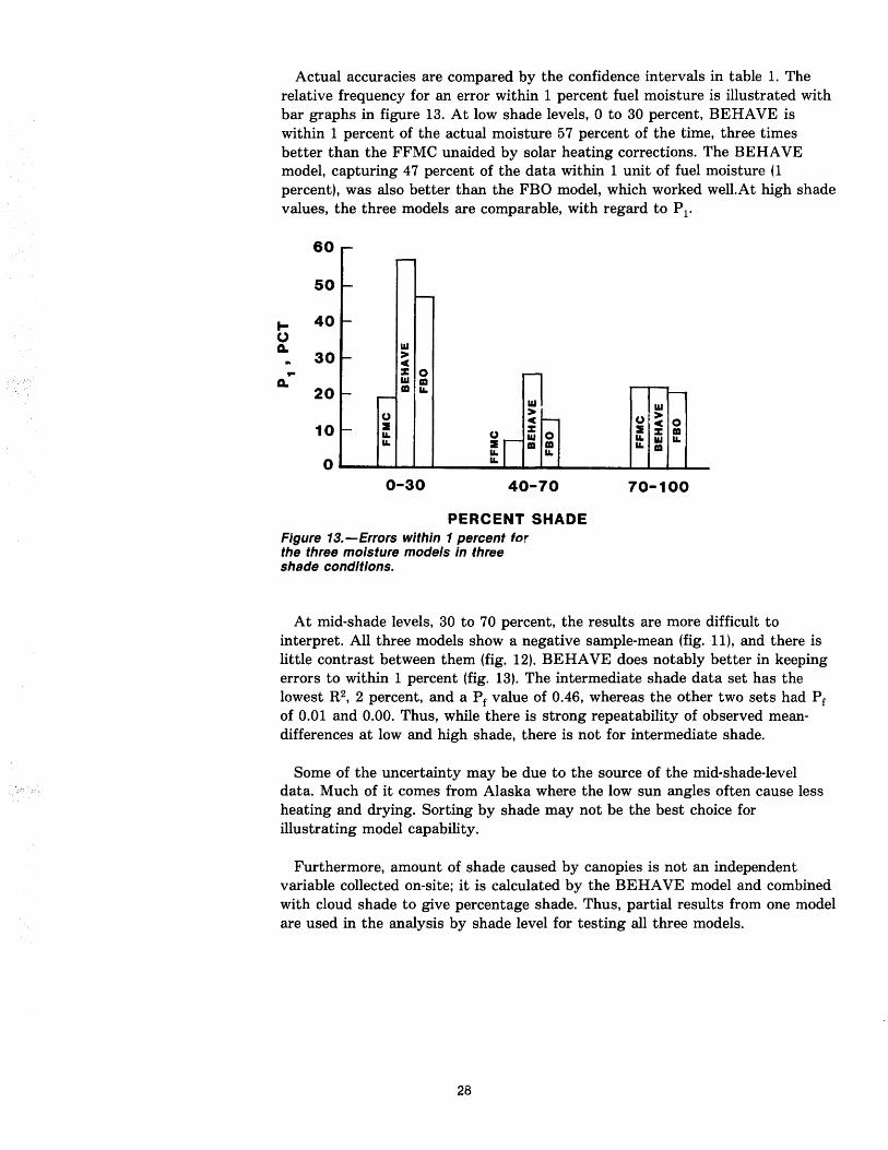
Actual accuracies are compared by the confidence intervals in table 1. The relative frequency for an error within 1 percent fuel moisture is illustrated with bar graphs in figure 13. At low shade levels, 0 to 30 percent, BEHAVE is within 1 percent of the actual moisture 57 percent of the time, three times better than the FFMC unaided by solar heating corrections. The BEHAVE model, capturing 47 percent of the data within 1 unit of fuel moisture (1 percent), was also better than the FBO model, which worked well.At high shade values, the three models are comparable, with regard to P l'

t­O a.

... a.

60

50

40

30

20

10

o

r--

I-

I-

-

I-

I-

-

~

W > c :c 0 r-W ID ID II.

r-- au CJ > 2 C -:c II.

~r w 0

II. ID ID II.

0-30 40-70

PERCENT SHADE Figure 13.-Errors within 1 percent for the three moisture models in three shade conditions.

~r--_

au > CJ C 0

:E :c ID II. W II. II. ID

70-100

At mid-shade levels, 30 to 70 percent, the results are more difficult to interpret. All three models show a negative sample-mean (fig. 11), and there is little contrast between them (fig. 12). BEHAVE does notably better in keeping errors to within 1 percent (fig. 13). The intermediate shade data set has the lowest R2, 2 percent, and a P f value of 0.46, whereas the other two sets had P f

of 0.01 and 0.00. Thus, while there is strong repeatability of observed mean­differences at low and high shade, there is not for intermediate shade.

Some of the uncertainty may be due to the source of the mid-shade-Ievel data. Much of it comes from Alaska where the low sun angles often cause less heating and drying. Sorting by shade may not be the best choice for illustrating model capability.

Furthermore, amount of shade caused by canopies is not an independent variable collected on-site; it is calculated by the BEHAVE model and combined with cloud shade to give percentage shade. Thus, partial results from one model are used in the analysis by shade level for testing all three models.

28

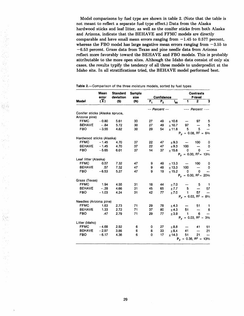
Model comparisons by fuel type are shown in table 2. (Note that the table is not meant to reflect a separate fuel type effect.) Data from the Alaska hardwood sticks and leaf litter, as well as the conifer sticks from both Alaska and Arizona, indicate that the BEHAVE and FFMC models are directly comparable and have small mean errors ranging from -1.45 to 0.577 percent, whereas the FBO model has large negative mean errors ranging from -3.55 to -6.53 percent. Grass data from Texas and pine needle data from Arizona reflect more favorably toward the BEHAVE and FBO models. This is probably attributable to the more open sites. Although the Idaho data consist of only six cases, the results typify the tendency of all three models to underpredict at the Idaho site. In all stratifications tried, the BEHAVE model performed best.

Table 2.-Comparison of the three moisture models, sorted by fuel types

Mean Standard Sample Contrasts error deviation size Confidence P·level

Model (X) (S) (N) P1 P3 IgO 2 3

-- Percent -- --- Percent ---Conifer sticks (Alaska spruce, Arizona pine)

FFMC -0.80 5.61 30 27 49 ±10.6 97 5 BEHAVE -.84 5.72 30 27 49 ±10.7 97 5 FBO -3.55 4.82 30 29 54 ± 11.8 5 5

PF = 0.08, R2 = 6%

Hardwood sticks (Alaska) FFMC -1.45 4.70 37 22 47 ±9.3 100 0 BEHAVE -1.45 4.70 37 22 47 ±9.3 100 0 FBO -5.65 6.01 37 14 37 ±15.6 0 0

PF = 0.00, R2= 13%

Leaf Iitter"(Alaska) FFMC 0.57 7.32 47 9 49 ±13.3 100 0 BEHAVE .57 7.32 47 9 49 ±13.3 100 0 FBO -6.53 5.27 47 9 19 ±15.2 0 0

PF = 0.00, R2 = 20%

Grass (Texas) FFMC 1.94 4.55 31 18 44 ±7.0 5 1 BEHAVE -.39 4.66 31 45 65 ±7.7 5 57 FBO -1.03 4.24 31 42 77 ±7.0 1 57

PF = 0.03, R2 = 8%

Needles (Arizona pine) FFMC 1.63 2.73 71 29 78 ±4.3 51 1 BEHAVE 1.33 2.72 71 37 80 ±4.3 51 6 FBO .47 2.79 71 29 77 ±3.9 1 6

PF = 0.03, R2 = 3%

Litter (Idaho) FFMC -4.68 2.92 6 0 27 ±8.8 41 51 BEHAVE -2.97 3.86 6 8 33 ±8.4 41 21 FBO -6.17 4.36 6 0 17 ±14.3 51 21

PF = 0.36, R2 = 13%

29

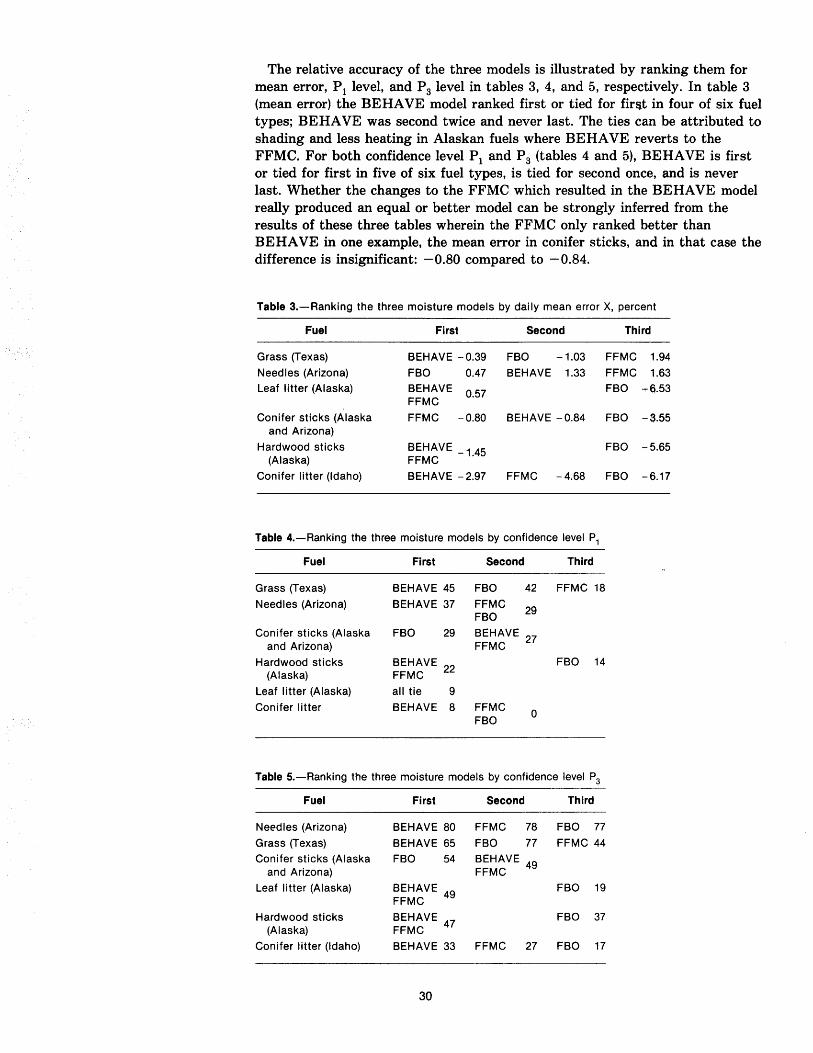
The relative accuracy of the three models is illustrated by ranking them for mean error, PI level, and Ps level in tables 3, 4, and 5, respectively. In table 3 (mean error) the BEHAVE model ranked first or tied for fir~t in four of six fuel types; BEHAVE was second twice and never last. The ties can be attributed to shading and less heating in Alaskan fuels where BEHAVE reverts to the FFMC. For both confidence level PI and Pa (tables 4 and 5), BEHAVE is first or tied for first in five of six fuel types, is tied for second once, and is never last. Whether the changes to the FFMC which resulted in the BEHAVE model really produced an equal or better model can be strongly inferred from the results of these three tables wherein the FFMC only ranked better than BEHA VE in one example, the mean error in conifer sticks, and in that case the difference is insignificant: -0.80 compared to -0.84.

Table 3.-Ranking the three moisture models by daily mean error X, percent

Fuel

Grass (Texas)

Needles (Arizona) Leaf litter (Alaska)

Conifer sticks (Alaska and Arizona)

Hardwood sticks (Alaska)

First

BEHAVE -0.39

FBD 0.47

BEHAVE 057 FFMC .

FFMC -0.80

BEHAVE -145 FFMC .

Second

FBD -1.03

BEHAVE 1.33

BEHAVE -0.84

Third

FFMC 1.94

FFMC 1.63 FBD .,6.53

FBD -3.55

FBD -5.65

Conifer litter (Idaho) BEHAVE -2.97 FFMC -4.68 FBD -6.17

Table 4.-Ranking the three moisture models by confidence level P1

Fuel First Second Third

Grass (Texas) BEHAVE 45 FBD 42 FFMC 18

Needles (Arizona) BEHAVE 37 FFMC 29

FBD

Conifer sticks (Alaska FBD 29 BEHAVE 27 and Arizona) FFMC

Hardwood sticks BEHAVE 22 FBD 14 (Alaska) FFMC

Leaf litter (Alaska) all tie 9 Conifer litter BEHAVE 8 FFMC

0 FBD

Table 5.-Ranking the three moisture models by confidence level P3

Fuel First Second Third

Needles (Arizona) BEHAVE 80 FFMC 78 FBD 77

Grass (Texas) BEHAVE 65 FBD 77 FFMC 44 Conifer sticks (Alaska FBD 54 BEHAVE 49

and Arizona) FFMC

Leaf litter (Alaska) BEHAVE 49 FBD 19 FFMC

Hardwood sticks BEHAVE 47 FBD 37 (Alaska) FFMC

Conifer litter (Idaho) BEHAVE 33 FFMC 27 FBD 17

30

Initialization Validation (Objective No.2)

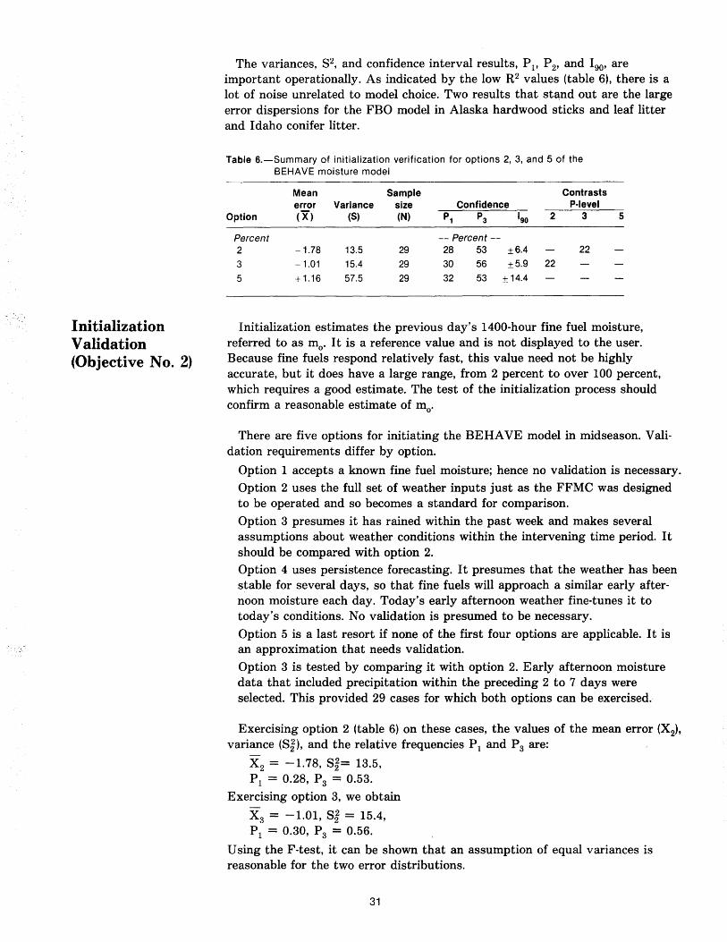
The variances, 82, and confidence interval results, P l' P 2' and 190, are important operationally. As indicated by the low R2 values (table 6), there is a lot of noise unrelated to model choice. Two results that stand out are the large error dispersions for the FBO model in Alaska hardwood sticks and leaf litter and Idaho conifer litter.

Table 6.-Summary of initialization verification for options 2, 3, and 5 of the BEHAVE moisture model

Mean Sample Contrasts error Variance size Confidence P·level

Option (X) (S) (N) P1 P3 190 2 3 5

Percent -- Percent --2 -1.78 13.5 29 28 53 ±6.4 22

3 -1.01 15.4 29 30 56 ±5.9 22

5 + 1.16 57.5 29 32 53 ±14.4

Initialization estimates the previous day's 1400-hour fine fuel moisture, referred to as mo' I t is a reference value and is not displayed to the user. Because fine fuels respond relatively fast, this value need not be highly accurate, but it does have a large range, from 2 percent to over 100 percent, which requires a good estimate. The test of the initialization process should confirm a reasonable estimate of mo'

There are five options for initiating the BEHAVE model in midseason. Vali-dation requirements differ by option.

Option 1 accepts a known fine fuel moisture; hence no validation is necessary. Option 2 uses the full set of weather inputs just as the FFMC was designed to be operated and so becomes a standard for comparison.

Option 3 presumes it has rained within the past week and makes several assumptions about weather conditions within the intervening time period. It should be compared with option 2. Option 4 uses persistence forecasting. It presumes that the weather has been stable for several days, so that fine fuels will approach a similar early after­noon moisture each day. Today's early afternoon weather fine-tunes it to today's conditions. No validation is presumed to be necessary.

Option 5 is a last resort if none of the first four options are applicable. It is an approximation that needs validation.

Option 3 is tested by comparing it with option 2. Early afternoon moisture data that included precipitation within the preceding 2 to 7 days were selected. This provided 29 cases for which both options can be exercised.

Exercising option 2 (table 6) on these cases, the values of the mean error (X2),

variance (8~), and the relative frequencies PI and P a are:

X 2 = -1. 78, 8~= 13.5, PI = 0.28, Pa = 0.53.

Exercising option 3, we obtain

Xa = -1.01, 8~ = 15.4, PI = 0.30, Pa = 0.56.

Using the F-test, it can be shown that an assumption of equal variances is reasonable for the two error distributions.

31

Validation of Diurnal Capability (Objective No.3)

The differences between the PI-values and between the P 3-values had P values of 0.59 and 0.48, respectively. This test is based on the binomial process with 29 trials. A Student-t statistic computed from X3 - X2 had a P value of 0.22.

In conclusion, option 3 is about as accurate (perhaps slightly better) on three of the four tests, having (perhaps) a slightly higher variance than option 2.

Initialization by use of option 5 was simulated by using the same 29 cases, but with the period length reduced to 1 day of propagation and the first fuel moisture set to 6, 16, or 76 percent. The three fuel moisture levels represent the three possible qualitative descriptions of the preceding week's weather. To simulate this, the equilibrium fuel moisture was computed for each day and averaged. The closest of the three moisture levels (6, 16, or 76) to this average was chosen as the initial value to use.

Exercising this simulated option 5:

X5 = 1.16, S2 = 57.5, PI = 0.32, P3 = 0.53

The F-ratio Sg/S~ is significant at <0.005; consequently, a meaningful compari­son of the mean errors of options 2 and 5 requires a different method. Assum­ing normally distributed mean errors and that the actual error variances are 13.4 and 57.5, respectively, then

(X2 - u)/(13.4/29)Y2 and (X5 - u)/(57.5/29)Y2

are normal random variables with a mean of zero and variance of 1. The hypothesis that X2 and X5 have the same mean (p.) can be tested. The sample values of these two standardized random variables are -0.48 and +0.48, respectively. The probability of that is (0.32)2 or 0.10; the means are different at a significance level of 10 percent. Differences between the PI- and P3-values are significant at 0.43 and 0.63, respectively, for the 29-trial binomial tests.

Option 5 generates errors having a mean which is quite different from that of option 2 and much greater variance. The scores PI and P 3 are not significantly different, however.

Based on rather noisy data, it is apparent that option 3 is as good as option 2, while only the large errors are worsened by the use of option 5 in place of option 2. Evidently, any difference between the true values of PI and P3 is sometimes masked by data noise if we assume that extra input information cannot harm model performance.

Validation of diurnal capability is concentrated on the BEHAVE model using the Canadian code with hourly prediction capability. This is because neither the FBO model nor the tables developed by the Canadian Forestry Service (Van Wagner 1972; Alexander 1982) for the FFMC have the forecasting capa­bilities needed for the BEHA VE system.

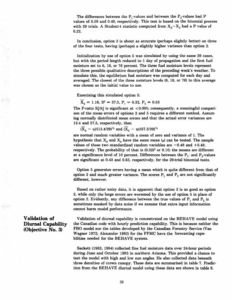
Sackett (1983, 1984) collected fine fuel moisture data over 24-hour periods during June and October 1983 in northern Arizona. This provided a chance to test the model with high and low sun angles. He also collected data beneath three densities of crown canopy. These data are summarized in table 7. Predic­tion from the BEHA VE diurnal model using these data are shown in table 8.

32

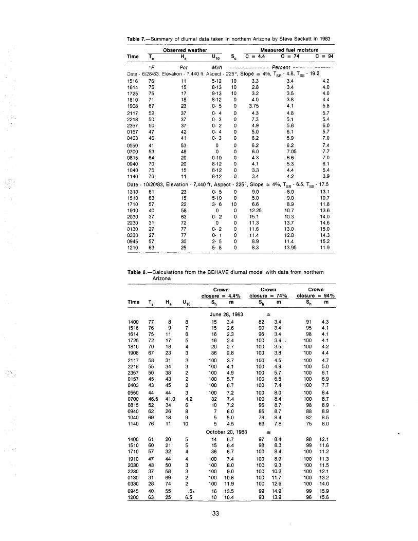
Table 7.-Summary of diurnal data taken in northern Arizona by Steve Sackett in 1983

Observed weather Measured fuel moisture Time Ta Ha U10 Sc C = 4.4 C = 74 C = 94

of Pct Milh --------------- Percent ---------------Date - 6/28/83, Elevation - 7,440 ft, Aspect - 225 0, Slope == 4%, T SR - 4_8, T ss - 19_2

1516 76 11 5-12 10 3.3 3.4 4.2 1614 75 15 8-13 10 2.8 3.4 4.0 1725 75 17 9-13 10 3.2 3.5 4.0 1810 71 18 8-12 0 4.0 3.8 4.4 1908 67 23 O· 5 0 3.75 4.1 5.8

2117 52 37 0- 4 0 4.3 4.8 5.7 2218 50 37 0- 3 0 7.3 5.1 5.4 2357 50 37 0- 2 0 4.9 5.8 6.0 0157 47 42 0- 4 0 5.0 6.1 5.7 0403 46 41 0- 3 0 6.2 5.9 7.0

0550 41 53 0 0 6.2 6.2 7.4 0700 53 48 0 0 6.0 7.05 7.7 0815 64 20 0-10 0 4.3 6.6 7.0 0940 70 20 8-12 0 4.1 5.3 6.1 1040 75 15 8-12 0 3.3 4.4 5.4 1140 76 11 8-12 0 3.4 4.2 3.9

Date - 10/20/83, Elevation - 7,440 ft, Aspect - 225°, Slope == 4%, TSR - 6.5, Tss - 17.5

1310 61 23 0- 5 0 9.0 8.0 13.1 1510 63 15 5-10 0 5.0 9.0 10.7 1710 57 22 3- 6 10 6.6 8.9 11.8 1910 40 58 0 0 12.25 10.7 13.6 2030 37 63 0- 2 0 15.1 10.3 14.0 2230 31 72 0 0 11.3 13.7 14.6 0130 27 77 0- 2 0 11.6 13.0 15.0 0330 27 77 0- 1 0 11.4 12.8 14.3 0945 57 30 2- 5 0 8.9 11.4 15.2 1210 63 25 5- 8 0 8.3 13.95 11.9

Table S.-Calculations from the BEHAVE diurnal model with data from northern Arizona

Crown Crown Crown closure = 4.4 % closure = 74% closure = 94%

Time Ta Ha U10 Sh m Sh m Sh m

June 28, 1983 -

1400 77 8 8 15 3.4 82 3.4 91 4.3 1516 76 9 7 15 2.6 90 3.4 95 4.1 1614 75 11 6 16 2.3 96 3.4 98 4.1 1725 72 17 5 16 2.4 100 3.4 100 4.1 1810 70 18 4 20 2.7 100 3.5 100 4.2 1908 67 23 3 36 2.8 100 3.8 100 4.4

2117 58 31 3 100 3.7 100 4.5 100 4.7 2218 55 34 3 100 4.1 100 4.9 100 5.0 2357 50 38 2 100 4.9 100 5.7 100 6.1 0157 45 43 2 100 5.7 100 6.5 100 6.9 0403 43 45 2 100 6.7 100 7.4 100 7.7

0550 44 44 3 100 7.2 100 8.0 100 8.4 0700 46.5 41.0 4.2 32 7.4 100 8.4 100 8.7 0815 52 34 6 10 7.2 95 8.7 98 8.9 0940 62 26 8 7 6.0 85 8.7 88 8.9 1040 69 18 9 5 5.0 76 8.4 82 8.5 1140 76 11 10 5 4.5 69 7.8 75 8.0

October 20, 1983 -1400 61 20 5 14 6.7 97 8.4 98 12.1 1510 60 21 5 15 6.4 98 8.3 99 11.6 1710 57 32 4 36 6.7 100 8.4 100 11.2

1910 47 44 4 100 7.4 100 8.9 100 11.3 2030 43 50 3 100 8.0 100 9.3 100 11.5 2230 37 58 3 100 9.0 100 10.2 100 12.1 0130 31 69 2 100 10.8 100 11.7 100 13.2 0330 28 74 2 100 11.9 100 12.6 100 14.0

0945 40 55 .5A 16 13.5 99 14.9 99 15.9 1200 63 25 6.5 10 10.4 93 13.9 96 15.6

33

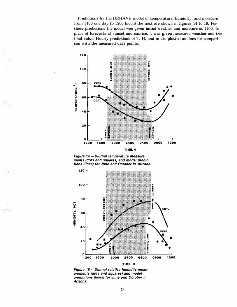
Predictions by the BEHAVE model of temperature, humidity, and moisture from 1400 one day to 1200 (noon) the next are shown in figures 14 to 18. For these predictions the model was given initial weather and moisture at 1400. In place of forecasts at sunset and sunrise, it was given measured weather and the final value. Hourly predictions of T, H, and m are plotted as lines for compari­son with the measured data points.

120

100

U- 80 0 iii' a: :) ... • c( 60 a: w A. :IE w ... 40

20

0 ___ 00l0000-__

1200 1600 2000 2400 0400 0800 1200

TIME,H

Figure 14.-Diurnal temperature measure­ments (dots and squares) and model predic­tions (lines) for June and October in Arizona.

120

100

80 t-(.) A.

,: 60 !:

c :IE :) :J:

40

• 20

o----'---~

iii ."

;~CT'

\ •

1200 1600 2000 2400 0400 0800 1200

TIME. H

Figure 15.-Diurnal relative humidity meas­urements (dots and squares) and model predictions (lines) for June and October in Arizona.

34

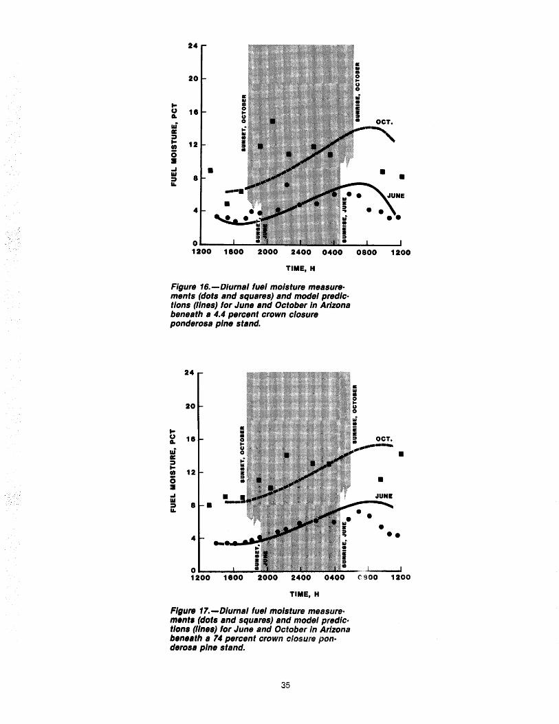
24

20

.. CJ 18 Ct.

ui CIC ~ ... 12 fI)

(5

• ~ • 1&1

8 ~ LL

4

0 ..... --...... __

1200 1800 2000 2400 0400 0800 1200

TIME, H

Figure 16. - Diurnal fuel moisture measure· ments (dots and squares) and model predic­tions (lines) for June and October In Arizona beneath a 4.4 percent crown closure ponderosa pine stand.

24

20

... CJ 18 Ct.

ui a: :::» ..

12 fI)

0 :I ~ 1&1

8 • ~ LL

4

OCT.

• •

• ••

o --~!----~ 1200 1800 2000 2400 0400 C 800 1200

TIME, H

Figure 17.-Dlurnal fuel moisture measure­ment. (dots and squares) and model predlc· tlons (lines) for June and October In Arizona beneath a 74 percent crown closure pon­derosa pine stand.

35

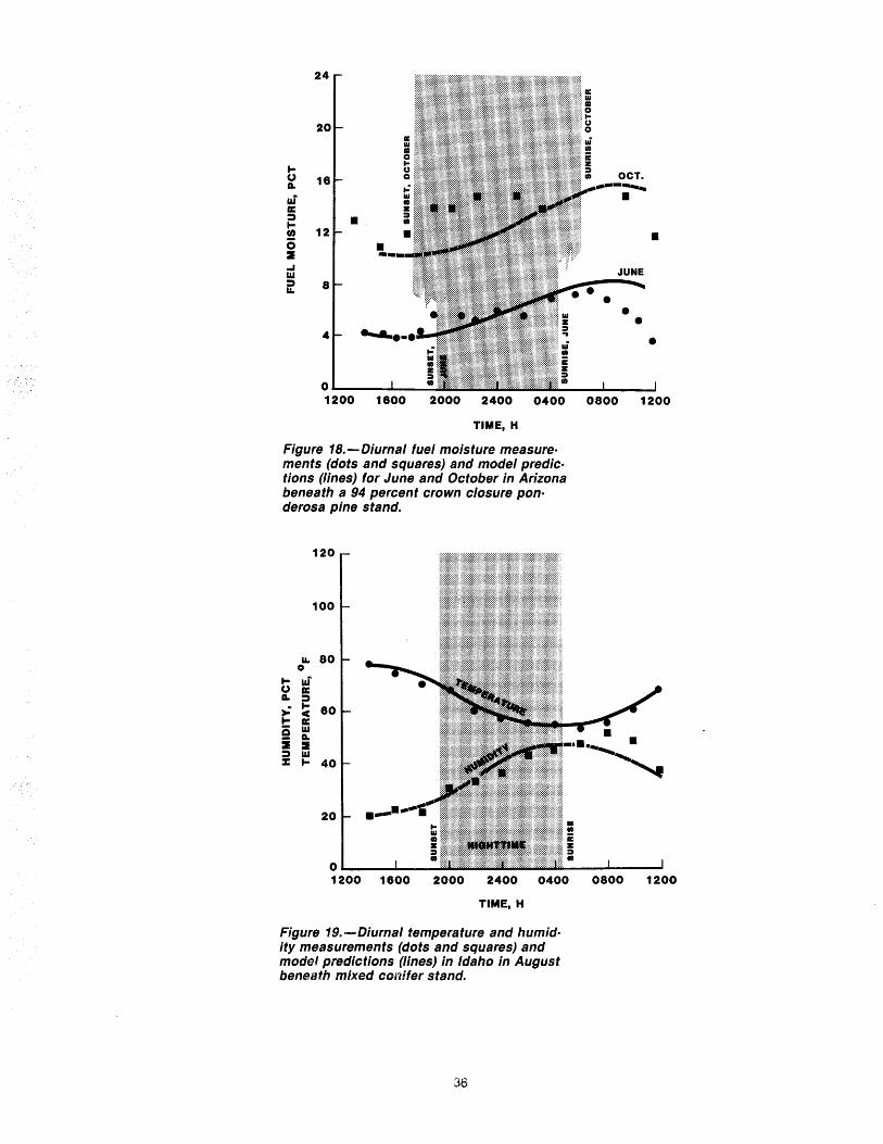
24

20

t-U 16 A.

W II: = • t-(/) 12 0 :I ... w = 8 &&.

4

0 ____ -... __ _

1200 1600 2000 2400 0400 0800 1200

TIME. H

Figure 18.-Diurnal fuel moisture measure· ments (dots and squares) and model predic· tions (lines) for June and October in Arizona beneath a 94 percent crown closure pon· derosa pine stand.

120

100

&&. 80 0

t- W U II: A. = > t- 60 C t- Il: 0 W

i A. :I = w :z: I- 40

20

0 ___ "",-__

1200 1600 2000 2400 0400

TIME. H

Figure 19.-Diurnal temperature and humid· ity measurements (dots and squares) and model predictions (lines) in Idaho in August beneath mixed conifer stand.

36

• •• • ~

0800 1200

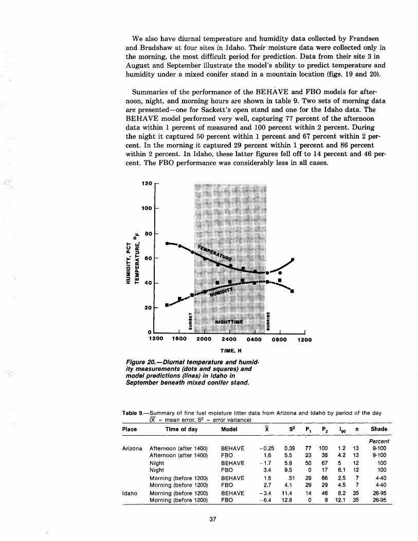
VVe also have diurnal temperature and humidity data collected by Frandsen and Bradshaw at four sites in Idaho. Their moisture data were collected only in the morning, the most difficult period for prediction. Data from their site 3 in August and September illustrate the model's ability to predict temperature and humidity under a mixed conifer stand in a mountain location (figs. 19 and 20).

Summaries of the performance of the BE HA VE and FBO models for after­noon, night, and morning hours are shown in table 9. Two sets of morning data are presented-one for Sackett's open stand and one for the Idaho data. The BEHAVE model performed very well, capturing 77 percent of the afternoon data within 1 percent of measured and 100 percent within 2 percent. During the night it captured 50 percent within 1 percent and 67 percent within 2 per­cent. In the morning it captured 29 percent within 1 percent and 86 percent within 2 percent. In Idaho, these latter figures fell off to 14 percent and 46 per­cent. The FBO performance was considerably less in all cases.

120

100

II. 80 0

t- iii (J a: a. :::I

> t- 60 ct t- a: Q 1&1

i a. :E :::» 1&1

% t- 40

20

o ---"-----' 1200 1600 2000 2400 0400 0800 1200

TIME. H

Figure 20.-Diurnal temperature and humid­ity measurements (dots and squares) and model predictions (lines) in Idaho in September beneath mixed conifer stand.

Table g.-Summary of fine fuel moisture litter data from Arizona and Idaho by period of the day (X = mean error, S2 = error variance)

Place Time of day Model X S2 P1 P2 IgO n Shade

Percent Arizona Afternoon (after 1400) BEHAVE -0.25 0.39 77 100 1.2 13 9·100

Afternoon (after 1400) FBO 1.6 5.5 23 38 4.2 13 9·100 Night BEHAVE -1.7 5.8 50 67 5 12 100 Night FBD 3.4 9.5 0 17 6.1 12 100 Morning (before 1200) BEHAVE 1.5 .51 29 86 2.5 7 4·40 Morning (before 1200) FBO 2.7 4.1 29 29 4.5 7 4·40

Idaho Morning (before 1200) BEHAVE -3.4 11.4 14 46 8.2 35 26·95 Morning (before 1200) FBO -6.4 12.8 0 9 12.1 35 26·95

37

The statistical summary indicates that the BEHAVE diurnal model performs very well. Figures 14 through 20 reveal more about its capabilities. Predictions of temperature and humidity through the late afternoon and night are surpris­ingly accurate, in both Arizona and Idaho. An exception may be in the predic­tions of temperature and humidity in October in Arizona. The trend of the actual data is followed, but through the night actual temperatures are about 50 cooler than predicted and humidities about 10 percent higher. As shown in the October fuel moisture predictions (figs. 16, 17, and 18), moisture is under­predicted during the night.

In the morning the model responds fastest for conditions in the open stand (fig. 16) because the solar heating functions bring the predicted fuel moisture down faster than in the shaded sites (figs. 17 and 18). More diurnal data are needed to determine if these effects are persistent enough to warrant changes to the model.

REFERENCES Albini, Frank A.; Baughman, Robert G. Estimating windspeeds for predicting

wildland fire behavior. Research Paper INT-221. Ogden, UT: U.S. Department of Agriculture, Forest Service, Intermountain Forest and Range Experiment Station; 1979. 12 p.

Albini, F. A. Computer-based models of wildland fire behavior: a users' manual. Ogden, UT: U.S. Department of Agriculture, Forest Service, Intermountain Forest and Range Experiment Station; 1976. 68 p.

Alexander, M. E. Diurnal adjustment table for the Fine Fuel Moisture Code. Forest Management Note No. 17. Edmonton, AB: Environment Canada, Canadian Forestry Service, Northern Forest Research Centre; 1982. 3 p.

Alexander, M. E.; Lee, B. S.; Lee, C. Y. Hourly calculation of the Fine Fuel Moisture Code, Initial Spread Index, and Fire Weather Index with the Texas Instruments model 59 hand-held calculator. Study NOR-5-191 File Report No. 7. Edmonton, AB: Agriculture Canada, Canadian Forestry Service, Northern Forest Research Centre; 1984. 17 p.

Anderson, H. E. Moisture and fine forest fuel response. In: Proceedings, eighth national conference on fire and forest meteorology; 1985 April 29-May 30; Detroit, MI. [In press].

Andrews, P. L. BEHAVE: fire behavior prediction and fuel modeling system­BURN subsystem. General Technical Report INT-194. Ogden, UT: Depart­ment of Agriculture, Forest Service, Intermountain Research Station; 1986.

Barbour, M. G.; Burk, J. H.; Pitts, W. D. Terrestrial plant ecology. Menlo Park, CA: Ben Cummings Publishing Company; 1980. 604 p.

Barrows, Jack S. Forest fires in the Northern Rocky Mountains. Station Paper No. 28. Missoula, MT: U.S. Department of Agriculture, Forest Service, Northern Rocky Mountain Forest and Range Experiment Station; 1951. 251 p.

Bates, C. G.; Henry, A. J. Forest and stream flow experiment at Wagon Wheel Gap, Colorado. Monthly Weather Review. 56(3): 79-85; 1928.

Buck, Arden L. New equations for computing vapor pressure and enhancement factor. Journal of Applied Meteorology. 20: 1527-1532; 1981.

Burgan, R. E.; Rothermel, R. C. BEHAVE: fire behavior prediction and fuel modeling system-FUEL subsystem. General Technical Report INT-167.

38

Ogden, UT: U.S. Department of Agriculture, Forest Service, Intermountain Forest and Range Experiment Station; 1984. 126 p.

Byram, G. M. Sun and wind and fuel moisture. Journal of Forestry. 38: 639-640; 1940.

Byram, G. M.; Jemison, G. M. Solar radiation and forest fuel moisture. Journal of Agricultural Research. 67(4): 149-176; 1943.

Canadian Forestry Service. Tables for the Canadian Forest Fire Weather Index System. Forestry Technical Report 25. Ottawa, ON: Environment Canada, Canadian Forestry Service; 1984. 48 p.

Catchpole, E. A.; Catchpole, W. R. Analysis of the 1972 Darwin grass fires. Report No.3. Duntroon, A.C.T., Australia: The University of New South Wales, Faculty of Military Studies, Department of Mathematics; 1983. 67 p.

Clark, Robert G. [Letters to Richard C. Rothermel]. 1981 September 2 and September 16.9 leaves and 151eaves. Located at: U.S. Department of Agriculture, Forest Service, Intermountain Forest and Range Experiment Station, Intermountain Fire Sciences Laboratory, Missoula, MT; RWU 2103 files.

Countryman, Clive M. Radiation effects on moisture in ponderosa pine litter. Research Paper PSW-126. Berkeley, CA: U.S. Department of Agriculture, Forest Service, Pacific Southwest Forest and Range Experiment Station; 1977. 23 p.

Deeming, John E.; Lancaster, James W.; Fosberg, Michael A.; Furman, R. William; Schroeder, Mark J. National Fire-Danger Rating System. Research Paper RM-84. Fort Collins, CO: U.S. Department of Agriculture, Forest Service, Rocky Mountain Forest and Range Experiment Station; 1972. 165 p.

Fischer, William C.; Hardy, Charles E. Fire-weather observers' handbook. Agriculture Handbook 494. Washington, DC: U.S. Department of Agriculture, Forest Service; 1976. 152 p.

Fosberg, Michael A.; Deeming, John E. Derivation of the 1- and 10-hour time­lag fuel moisture calculations for fire-danger rating. Research Note RM-207. Fort Collins, CO: U.S. Department of Agriculture, Forest Service, Rocky Mountain Forest and Range Experiment Station; 1971. 8 p.

Frandsen, W. H.; Bradshaw, L. Estimating duff moisture from meteorological measurements. In: Proceedings, sixth conference on fire and forest meteorology; 1980 April 22-24; Seattle, W A. Washington, DC: Society of American Foresters; 1980: 96-101.

Frank, E. C.; Lee, R. Potential solar beam irradiation on slopes: tables for 30 0

to 50 0 latitude. Research Paper RM-18. Fort Collins, CO: U.S. Department of Agriculture, Forest Service, Rocky Mountain Forest and Range Experiment Station; 1966. 116 p.

Gast, P. R.; Stickel, P. W. Solar radiation and relative humidity in relation to duff moisture and forest fire hazard. Monthly Weather Review. 1929 November 7: 466-468.

Gisbome, H. T. Measuring forest fire danger in northern Idaho. Miscellaneous Publication No. 29. Washington, DC: U.S. Department of Agriculture; 1928. 63 p.

Gisborne, H. T. Deadwood lying on duff drier than in air. Journal of Forestry. 31(8): 979-980; 1933.

Gisborne, H. T. The principles of measuring forest fire danger. Journal of Forestry. 34: 786-793; 1936.

Harrington, M. G. [Letter to Richard C. Rothermel]. 1983 July 6. 6 leaves. Located at: U.S. Department of Agriculture, Forest Service, Intermountain

39

Forest and Range Experiment Station, Intermountain Fire Sciences Laboratory, Missoula, MT; RWU 2103 files.

Hornby, L. G. Fuel type mapping in Region One. Journal of Forestry. 33: 67-72; 1935.

Johnson, J. C. Physical meteorology. 2d ed. New York: J. Wiley & Sons; 1960. 393 p.

Jordan, C. F. Derivation of leaf-area index from quality of light on the forest floor. Ecology. 50: 663-666; 1969.

Kaufmann, M. R.; Weatherred, J. D. Determination of potential direct beam solar irradiance. Research Paper RM-242. Fort Collins, CO: U.S. Department of Agriculture, Forest Service, Rocky Mountain Forest and Range Experi­ment Station; 1982. 23 p.

Kimball, H. H. Variations in the total and luminous solar radiation with geographical position in the United States. Monthly Weather Review. 47(11): 769-793; 1919.

Kondratyev, K. Ya. Radiation in the atmosphere. New York: Academic Press; 1969.912 p.

Lee, R. Theory of the "Equivalent Slope." Monthly Weather Review. 90: 165-166; 1962.

List, R. J. Smithsonian m.eteorological tables. 6th ed. Washington, DC: Smithsonian Institute Publishing Company; 1958. 527 p.

Loewe, F. The intake of solar radiation by slopes with cloudless sky. Bulletin No. 45. Melbourne: Commonwealth of Australia, Bureau of Meteorology; 1962. 57 p.

Luke, R. H.; McArthur, A. G. Bushfires in Australia. Canberra, Australia: Australian Government Publishing Service; 1978. 359 p.

Milankovetch, M. Mathematische Klimalehre. Handbuch der Klimatologische, Bank I, Teil A: 1-176; 1930.

Monsi, M.; Saeki, T. Uber den Lichtfaktor in den Pflanzengesellschaften und seine Bedeutung fur die Stoffproduktion. Japanese Journal of Botany. 14: 22-52; 1953.

Muraro, S. J.; Russel, R. N.; Lawson, B. D. Development of diurnal adjustments table for the Fine Fuel Moisture Code. Information Report BC-X-35. Victoria, BC: Department of Fisheries and Forestry, Forest Research Laboratory; 1969. 24 p.

Norum, Rodney A. [Letter to Richard C. Rothermel]. 1983 February 22. 29 leaves. Located at: U.S. Department of Agriculture, Forest Service, Intermountain Forest and Range Experiment Station, Intermountain Fire Sciences Laboratory, Missoula, MT.

Okanoue, Masco. On the intensity of solar radiation on any slope. Japanese Forestry Society Journal. 39(11): 435-437; 1957.

Pfister, R. D.; Kovalchik, B. L.; Arno, S. F.; Presby, R. C. Forest habitat types of M(>ntana. General Technical Report INT-34. Ogden, UT: U.S. Department of Agriculture, Forest Service, Intermountain Forest and Range Experiment Station; 1977. 174 p.

Plulnmer, F. G. Forest fires: their causes, extent, and effects, with a summary of recorded destruction and loss. Forest Service Bulletin 117. Washington, DC: U.S. Department of Agriculture; 1912. 39 p.

Rothermel, Richard C. A mathematical model for predicting fire spread in wildland fuels. Research Paper INT-115. Ogden, UT: U.S. Department of Agriculture, Forest Service, Intermountain Forest and Range Experiment Station; 1972. 40 p.

40

Rothermel, Richard C. How to predict the spread and intensity of forest and range fires. General Technical Report INT-143. Ogden, UT: U.S. Department of Agriculture, Forest Service, Intermountain Forest and Range Experiment Station; 1983. 161 p.

Running, Steven W.; Hungerford, Roger D. Spatial extrapolation of meteorological data for ecosystem modeling applications. In: Proceedings, 16th conference on agriculture and forest meteorology; 1983 April 25-29; Fort Collins, CO. Boston, MA: American Meteorological Society; 1983: 4 p., unnumbered proceedings.

Sackett, Stephen S. [Letters to Richard C. Rothermel]. 1983 September 10, 4 leaves and 1984 January 10, 5 leaves. Located at: U.S. Department of Agriculture, Forest Service, Intermountain Forest and Range Experiment Station, Intermountain Fire Sciences Laboratory, Missoula, MT; RWU 2103 files.

Salomon, R. M.; Ffolliott, P. F.; Thompson, J. R. Correlation between transmissivity and basal area in Arizona ponderosa pine forests. Research Note RM-318. Fort Collins, CO: U.S. Department of Agriculture, Forest Service, Rocky Mountain Forest and Range Experiment Station; 1976. 2 p.

Satterlund, D. R. Forest shadows: how much shelter in a shelterwood? Forest Ecology and Management. 5: 27-37; 1983.

Schroeder, Mark J.; Buck, Charles C. Fire weather ... a guide for application of meteorological information to forest fire control operations. Agriculture Handbook 360. Washington, DC; U.S. Department of Agriculture; 1970. 229 p.

Simard, A. J. [Letter to Richard C. Rothermel]. 1984 October 3. 2 leaves. Located at: U.S. Department of Agriculture, Forest Service, Intermountain Forest and Range Experiment Station, Intermountain Fire Sciences Laboratory, Missoula, MT; RWU 2103 files.

Simard, A. J.; Main, W. A. Comparing methods of predicting jack pine slash moisture. Canadian Journal of Forest Research. 12(4): 793-802; 1982.

Stage, A. R. An expression for the effect of aspect, slope, and habitat type on tree growth. Forest Science. 22(4): 457-460; 1976.

Turner, J. A.; Lawson, B. D. Weather in the Canadian Forest Fire Danger Rating System. Information Report BC-X-177. Victoria, BC: Pacific Forest Research Centre; 1978. 40 p.

Van Wagner, C. E. Combined effect of sun and wind on surface temperature of litter. Information Report PS-X-10. Chalk River, ON: Forestry Branch, Department of Fisheries and Forestry, Petawawa Forest Experiment Station; 1969.7 p.

Van Wagner, C. E. A table of diurnal variation in the Fine Fuel Moisture Code. Information Report PS-X-38. Chalk River, ON: Environment Canada, Canadian Forestry Service, Petawawa Forest Experiment Station; 1972. 8 p.

Van Wagner, C. E. Structure of the Canadian Forest Fire Weather Index. Publication No."1333. Ottawa, ON: Environment Canada, Canadian Forestry Service; 1974. 44 p.

Van Wagner, C. E. A method of computing fine fuel moisture content throughout the diurnal cycle. Information Report PS-X-69. Chalk River, ON: Fisheries and Environment Canada, Canadian Forestry Service, Petawawa Forest Experiment Station; 1977. 15 p.

Zavitkovski, J. Biomass studies in intensively managed forest stands. General Technical Report NC-21. St. Paul, MN: U.S. Department of Agriculture, Forest Service, North Central Forest Experiment Station; 1976. 117 p.

41

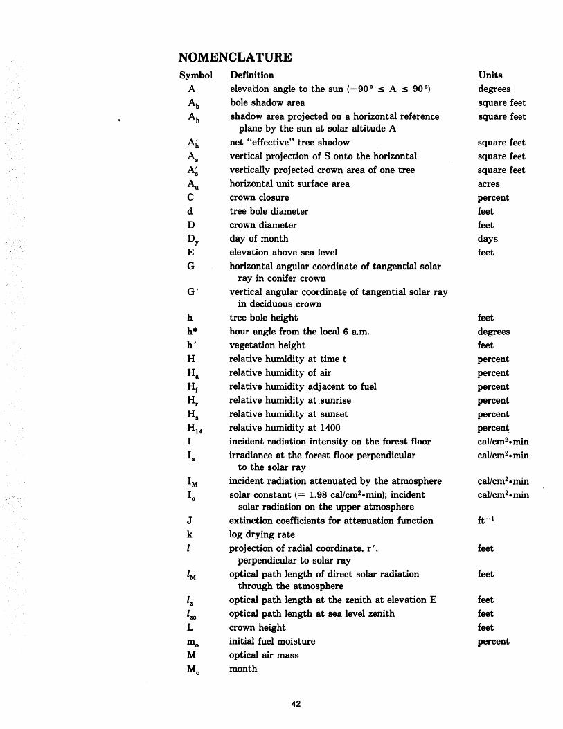
NOMENCLATURE

G'

h h* hi

H

Ha Hf

Hr Hs

H14

I

Ia

J k 1

Definition

elevation angle to the sun (-90 0 s A s 90 0)

bole shadow area shadow area projected on a horizontal reference

plane by the sun at solar altitude A net "effective" tree shadow vertical projection of S onto the horizontal vertically proj ected crown area of one tree horizontal unit surface area crown closure tree bole diameter crown diameter day of month elevation above sea level horizontal angular coordinate of tangential solar

ray in conifer crown vertical angular coordinate of tangential solar ray

in deciduous crown tree bole height hour angle from the local 6 a.m. vegetation height relative humidity at time t relative humidity of air relative humidity adjacent to fuel relative humidity at .sunrise relative humidity at sunset relative humidity at 1400 incident radiation intensity on the forest floor irradiance at the forest floor perpendicular

to the solar ray incident radiation attenuated by the atmosphere solar constant (= 1.98 cal/cm2.min); incident

solar radiation on the upper atmosphere extinction coefficients for attenuation function log drying rate proj ection of radial coordinate, r I ,

perpendicular to solar ray optical path length of direct solar radiation

through the atmosphere optical path length at the zenith at elevation E optical path length at sea level zenith crown height initial fuel moisture optical air mass month

42

Units

degrees square feet square feet

square feet square feet square feet acres percent feet feet days feet

feet degrees feet percent percent percent percent percent percen~

callcm2.min cal/cm2.min

cal/cm2·min cal/cm2• min

ft- I

feet

feet

feet feet feet percent

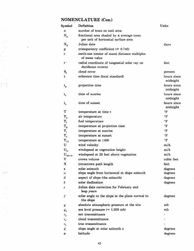
NOMENCLATURE (Con.) Symbol Definition Units

n number of trees on unit area

Nn fractional area shaded by n average trees per unit of horizontal surface area

NJ Julian date days p transparency coefficient (= 0.745)

r earth-sun (center of mass) distance multiples of mean value

r' radial coordinate of tangential solar rayon feet deciduous crowns

Sc cloud cover percent

t reference time (local standard) hours since midnight

tp projection time hours since midnight

tr time of sunrise hours since midnight

ts time of sunset hours since midnight

T temperature at time t of

Ta air temperature of

Tf fuel temperature of

Tp temperature at projection time of

Tr temperature at sunrise of

Ts temperature at sunset of

T14 temperature at 1400 of

U wind velocity mi/h Uh , windspeed at vegetation height mi/h

U 20+h , windspeed at 20 feet above vegetation mi/h V crown volume cubic feet X intracrown path length feet

z solar azimuth degrees a slope angle from horizontal at slope azimuth degrees {3 aspect of slope (the azimuth) degrees {) solar declination degrees

€ Julian date correction for February and leap years

r solar angle to the slope in the plane normal to degrees the slope

e absolute atmospheric pressure at the site mb

eo sea level pressure (= 1,000 mb) mb

Tn net transmittance

Tc cloud transmittance

Tt tree transmittance

I/; slope angle at solar azimuth z degrees

c/> latitude degrees

43

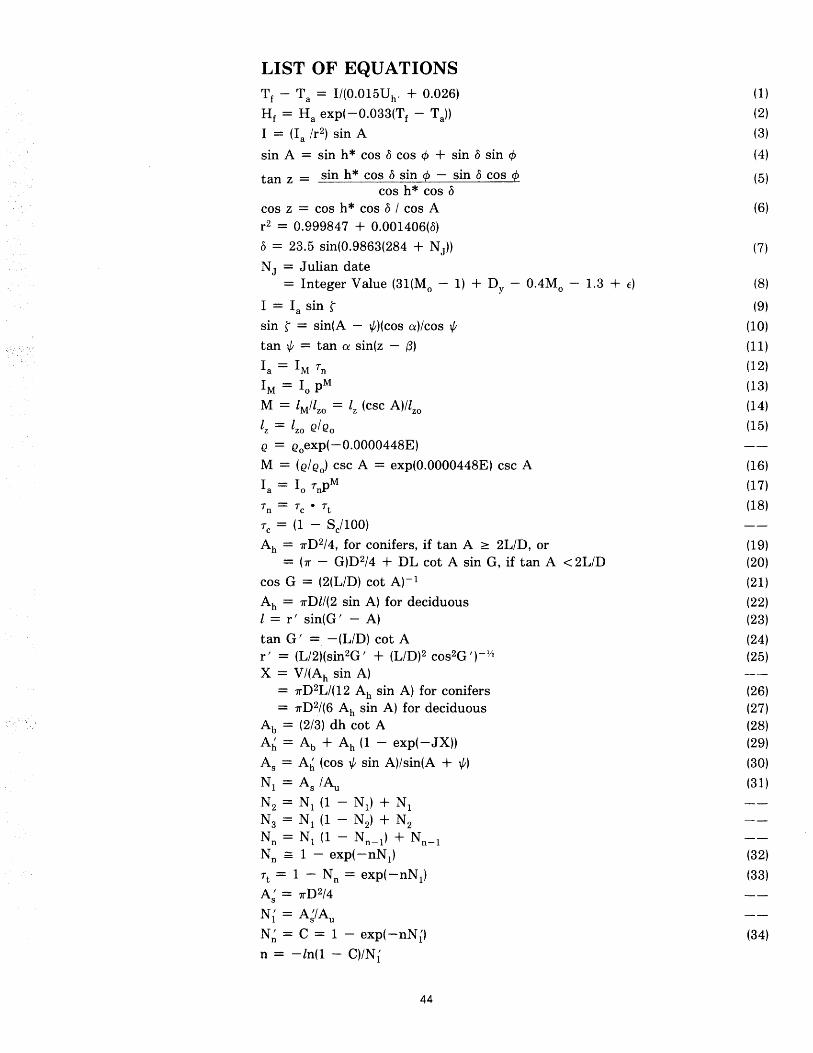
LIST OF EQUATIONS T f - Ta = I1(0.015Uh, + 0.026)

H f = Ha exp(-0.033(Tf - Ta))

I = (la Ir2) sin A

sin A = sin h * cos D cos cf> + sin D sin cf>

tan z = sin h * cos D sin cf> - sin D cos cf> cos h* cos D

cos z = cos h * cos D I cos A r2 = 0.999847 + 0.001406(D)

D = 23.5 sin(0.9863(284 + NJ ))

NJ = Julian date = Integer Value (31(Mo - 1) + Dy - O.4Mo - 1.3 + E)

I = la sin r sin r = sin(A - ~)(cos ex)/cos ~

tan ~ = tan ex sin(z - (3)

la = 1M Tn

1M = 10 pM

M = lM/lzo = lz (CSC A)llzo lz = lzo Qlc20

Q = Qoexp( -0.0000448E)

M = (QIQo) csc A = exp(0.0000448E) csc A

la = 10 TnpM

Tn = Tc • Tt

Tc = (1 - ScIlOO)

Ah = 7rD2/4, for conifers, if tan A ~ 2L/D, or = (7r - G)D2/4 + DL cot A sin G, if tan A < 2L/D

cos G = (2(L/D) cot A)-l

Ah = 7rDl/(2 sin A) for deciduous l = r' sin(G' - A)

tan G' = -(LID) cot A r' = (L/2)(sin2G' + (L/D)2 cos2G,)_1/2

X = V/(Ah sin A) = 7r D2L/( 12 Ah sin A) for conifers = 7rD2/(6 Ah sin A) for deciduous

Ab = (213) dh cot A Ah = Ab + Ah (1 - exp( -JX))

As = Ah (cos ~ sin A)/sin(A + ~) Nl = As IAu

N2 = Nl (1 - N1) + Nl N 3 = N 1 (1 - N 2) + N 2 Nn = Nl (1 - Nn- 1) + Nn- 1

Nn == 1 - exp(-nN1)

Tt = 1 - Nn = exp(-nN1)

A; = 7rD2/4

N{ = A;/Au

N~ = C = 1 - exp(-nN{)

n = -In(1 - C)/N {

44

(1) (2)

(3)

(4)

(5)

(6)

(7)

(8)

(9)

(10)

(11)

(12)

(13)

(14)

(15)

(16)

(17)

(18)

(19)

(20)

(21)

(22)

(23)

(24) (25)

(26) (27) (28) (29)

(30)

(31)

(32)

(33)

(34)

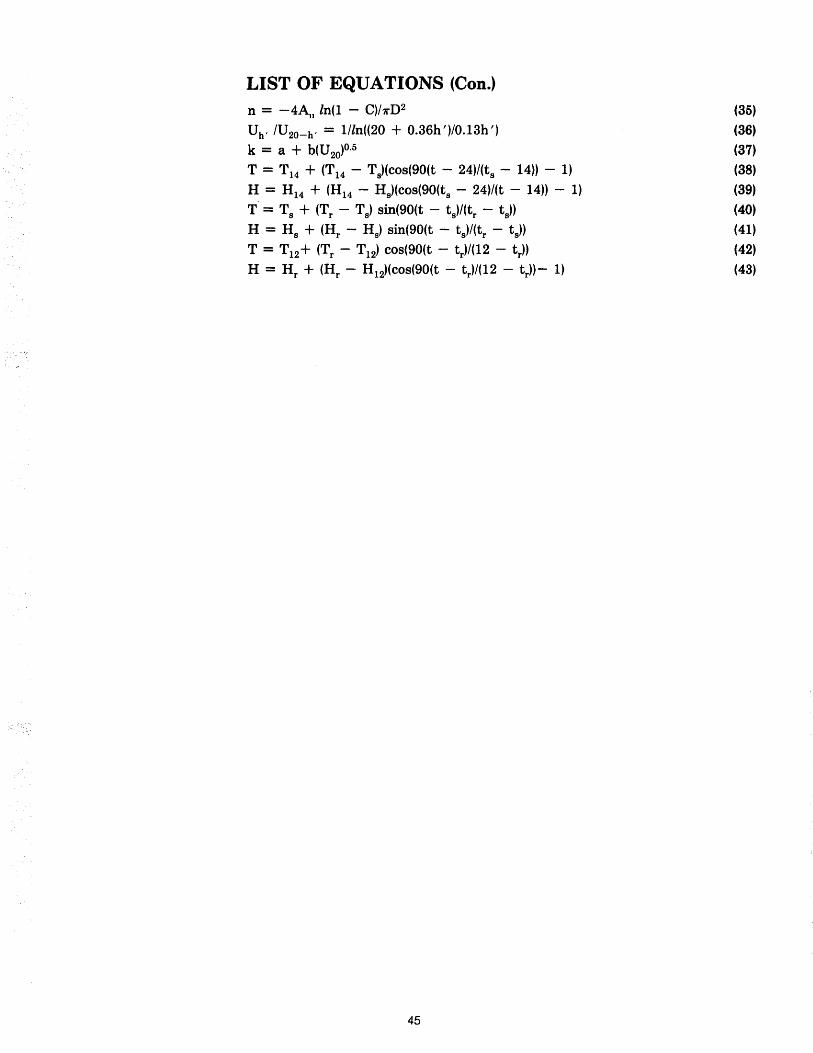
LIST OF EQUATIONS (Con.) n = -4~1 In(l - C)/1f'D2

Uh , IU20- h , = 1I1n((20 + O.36h')/0.13h')

k = a + b(U 20)°·5

T = T 14 + (T 14 - Ts)(cos(90(t - 24)/(ts - 14)) - 1)

H = H14 + (H14 - Hs)(cos(90(ts - 24)/(t - 14)) - 1)

T = Ts + (Tr - Ts) sin(90(t - ts)/(tr - t s))

H = Hs + (Hr - Hs) sin(90(t - ts)/(tr - t s))

T = T 12+ (Tr - T 12) cos(90(t - t r)/(12 - t r))

H = Hr + (Hr - H 12)(cos(90(t .;.... t r)/(12 - t r))- 1)

45

(35)

(36)

(37)

(38)

(39)

(40)

(41)

(42)

(43)

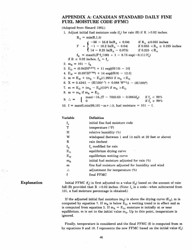
Explanation

APPENDIX A: CANADIAN STANDARD DAILY FINE FUEL MOISTURE CODE (FFMC) (Adapted from Simard 1982.)

1. Adjust initial fuel moisture code (fo) for rain (R) if R > 0.02 inches.

RA = min(R,1.5)

{

-56 - 55.6 In(RA + 0.04) if RA S 0.055 inches F = -1 - 18.2 In(RA - 0.04) if 0.055 < RA ~ 0.225 inches

14 - 8.25 In(RA - 0.075) if 0.225 <RA

fR = max(0,(F·fo/100) + 1 - 8.73 exp(-0.1117fo) if R ~ 0.02 inches, fR = fo.

2. mR = 101 - fR 3. En = (0.942Ho.679) + 11 exp[(H/10) - 10]

4. Ew = (0.597Ho.768) + 14 exp[(H/8) - 12.5]

5. m = Ew + (mR - Ew)/1.9953 if mR < En 6. X = 0.424(1 - (HIl00)1.7) + 0.088 WO.5(l - (H/100)8)

7. m = En + (mR - En)/(lOX) if mR > En

8. m = mR if mR = En

{ mO ax( -16.,(T - 70)(0.63 - 0.0065fR)

9. 6. = if fo < 99% if fo ~ 99%

10. f = max(0,min(99,101-m+ 6.)), fuel moisture = 101 - f.

Variable

fo T H

W

R

fR

En

Ew mR

m

6.

f

Definition

initial fine fuel moisture code

temperature (OF)

relative humidity (%)

windspeed (between 1 and 14 mi/h at 20 feet or above)

rain (inches)

fo modified for rain

equilibrium drying curve

equilibrium wetting curve

initial fuel moisture adjusted for rain (%)

fine fuel moisture adjusted for humidity and wind

adjustment for temperature (%)

final FFMC

Initial FFMC (fo) is first adjusted to a value (fR) based on the amount of rain­fall (R) provided that R >0.02 inches. (Note: fo is a code-when subtracted from 101, a fuel moisture percentage is obtained.)

If the adjusted initial fuel moisture (mR) is above the drying curve (En)' m is computed by equation 7. If mR is below En' a wetting trend is in effect and m is computed from equation 5. If mR = En' moisture is initially at or near equilibrium. m is set to the initial value mR. Up to this point, temperature is ignored. .

Finally, temperature is considered and the final FFMC (f) is computed from m by equations 9 and 10. f represents the new FFMC based on the initial value (fo)·

46

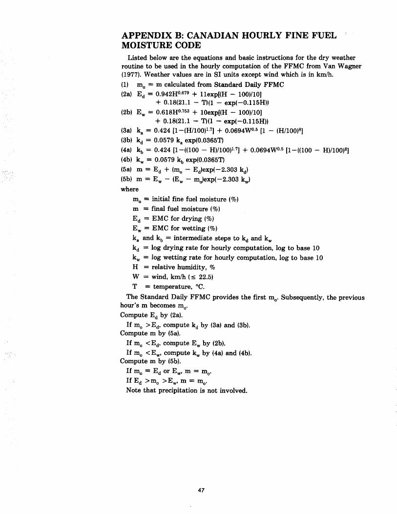
APPENDIX B: CANADIAN HOURLY FINE FUEL MOISTURE CODE

Listed below are the equations and basic instructions for the dry weather routine to be used in the hourly computation of the FFMC from Van Wagner (1977). Weather values are in SI units except wind which is in kmlh.

(1) mo = m calculated from Standard Daily FFMC (2a) Ed = 0.942Ho.679 + llexp[(H - 100)/10]

+ 0.18(21.1 - T)(1 - exp(-0.115H)) (2b) Ew = 0.618Ho.753 + 10exp[(H - 100)/10]

+ 0.18(21.1 - T)(1 - exp(-0.115H)) (3a) ka = 0.424 [1-(H/I00)1.7] + 0.0694Wo.5 [1 - (H/I00)8]

(3b) kd = 0.0579 ka exp(0.0365T) (4a) kb = 0.424 [1-((100 - H)/I00)1.7] + 0.0694Wo.5 [1-((100 - H)/I00)8]

(4b) kw = 0.0579 kb exp(0.0365T)

(5a) m = Ed + (mo - Ed)exp( - 2.303 kd) (5b) m = Ew - (Ew - mo)exp(-2.303 kw)

where

mo = initial fine fuel moisture (%)

m = final fuel moisture (%)

Ed = EMC for drying (%)

Ew = EMC for wetting (%)

ka and kb = intermediate steps to kd and kw kd = log drying rate for hourly computation, log to base 10 kw = log wetting rate for hourly computation, log to base 10 H = relative humidity, %

W = wind, kmlh (s 22.5)

T = temperature, °C.

The Standard Daily FFMC provides the first mo' Subsequently, the previous hour's m becomes mo' Compute Ed by (2a).

If mo > Ed' compute kd by (3a) and (3b). Compute m by (5a).

If mo < Ed' compute Ew by (2b). If mo < Ew' compute kw by (4a) and (4b).

Compute m by (5b).

If mo = Ed or Ew' m = mo'

If Ed >mo >Ew' m = mo' Note that precipitation is not involved.

47

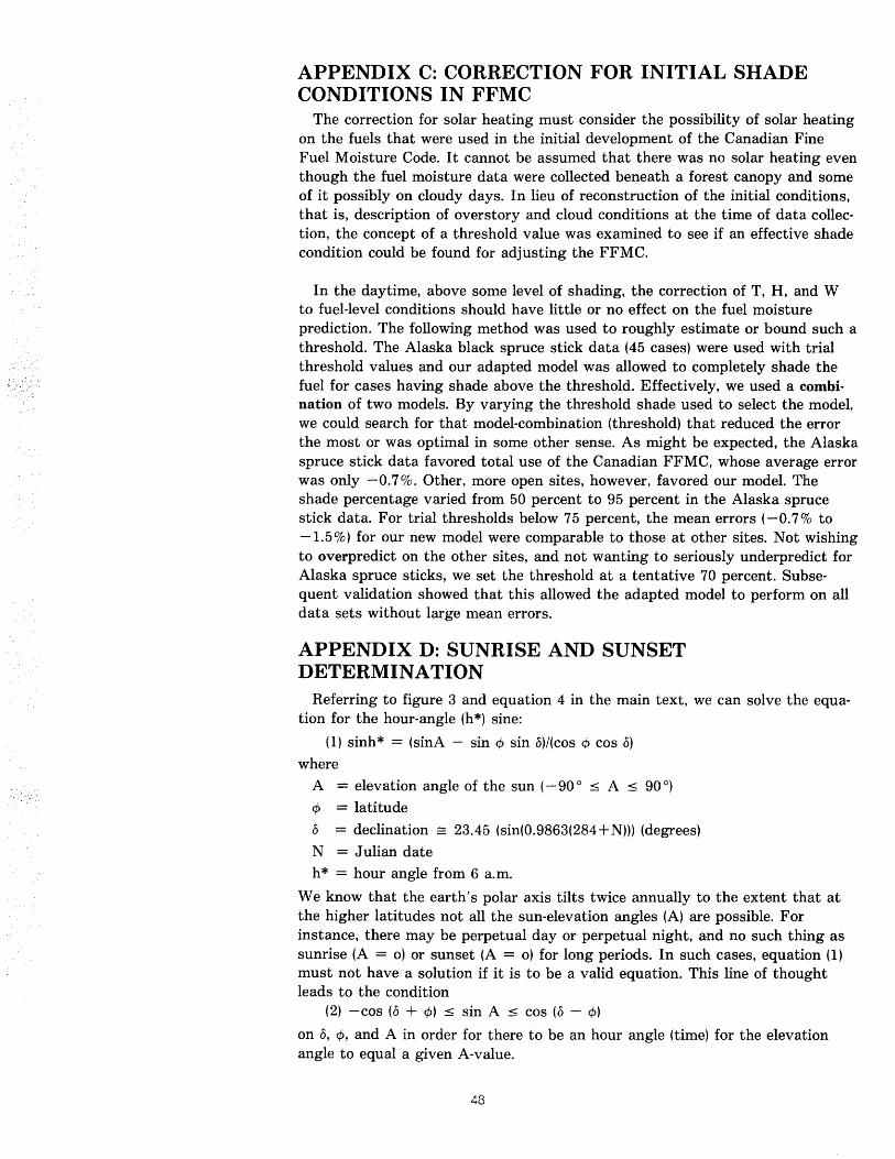
APPENDIX C: CORRECTION FOR INITIAL SHADE CONDITIONS IN FFMC

The correction for solar heating must consider the possibility of solar heating on the fuels that were used in the initial development of the Canadian Fine Fuel Moisture Code. I t cannot be assumed that there was no solar heating even though the fuel moisture data were collected beneath a forest canopy and some of it possibly on cloudy days. In lieu of reconstruction of the initial conditions, that is, description of overs tory and cloud conditions at the time of data collec­tion, the concept of a threshold value was examined to see if an effective shade condition could be found for adjusting the FFMC.

In the daytime, above some level of shading, the correction of T, H, and W to fuel-level conditions should have little or no effect on the fuel moisture prediction. The following method was used to roughly estimate or bound such a threshold. The Alaska black spruce stick data (45 cases) were used with trial threshold values and our adapted model was allowed to completely shade the fuel for cases having shade above the threshold. Effectively, we used a combi­nation of two models. By varying the threshold shade used to select the model, we could search for that model-combination (threshold) that reduced the error the most or was optimal in some other sense. As might be expected, the Alaska spruce stick data favored total use of the Canadian FFMC, whose average error was only -0.7%. Other, more open sites, however, favored our model. The shade percentage varied from 50 percent to 95 percent in the Alaska spruce stick data. For trial thresholds below 75 percent, the mean errors (-0.7% to -1.5%) for our new model were comparable to those at other sites. Not wishing to overpredict on the other sites, and not wanting to seriously underpredict for Alaska spruce sticks, we set the threshold at a tentative 70 percent. Subse­quent validation showed that this allowed the adapted model to perform on all data sets without large mean errors.

APPENDIX D: SUNRISE AND SUNSET DETERMINATION

Referring to figure 3 and equation 4 in the main text, we can solve the equa­tion for the hour-angle (h *) sine:

(1) sinh* = (sinA - sin ¢ sin o)/(cos ¢ cos 0)

where A = elevation angle of the sun (-90 0

::; A ::; 90 0)

¢ = latitude

o = declination == 23.45 (sin(0.9863(284+ N))) (degrees)

N = Julian date h* = hour angle from 6 a.m.

We know that the earth's polar axis tilts twice annually to the extent that at the higher latitudes not all the sun-elevation angles (A) are possible. For instance, there may be perpetual day or perpetual night, and no such thing as sunrise (A = 0) or sunset (A = 0) for long periods. In such cases, equation (1) must not have a solution if it is to be a valid equation. This line of thought leads to the condition

(2) -cos (0 + ¢) ::; sin A ::; cos (0 - ¢)

on 0, ¢, and A in order for there to be an hour angle (time) for the elevation angle to equal a given A-value.

48

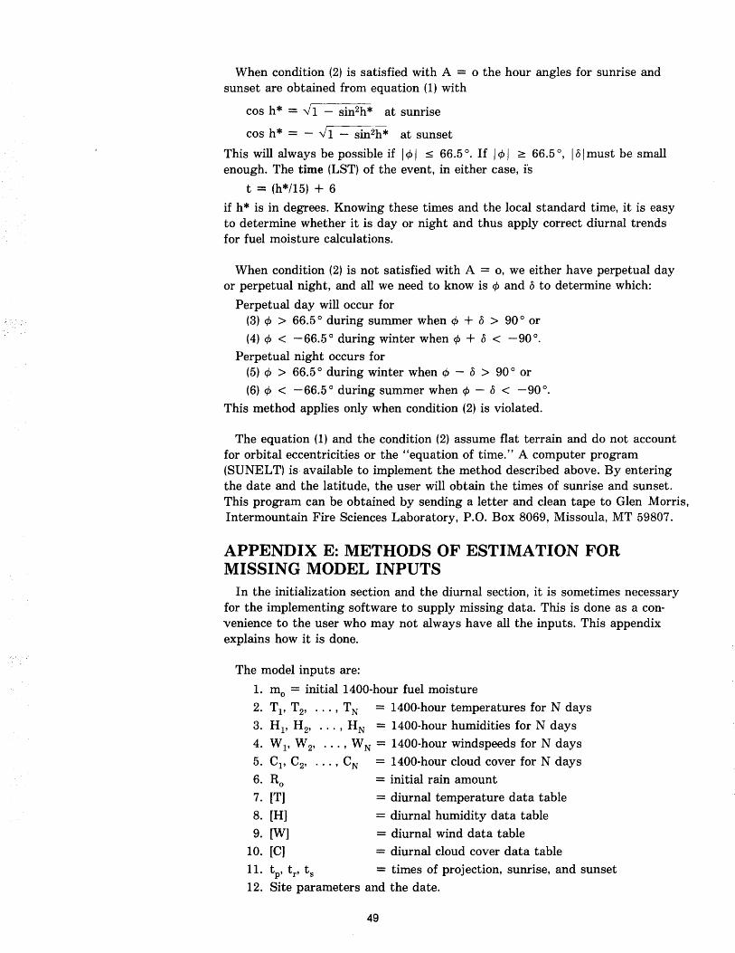
When condition (2) is satisfied with A = 0 the hour angles for sunrise and sunset are obtained from equation (1) with

cos h* = "';1 - sin2h* at sunrise

cos h* = - "';1 - sin2h* at sunset

This will always be possible if I cf> I ~ 66.5°. If I cf> I ~ 66.5°, 10 I must be small enough. The time (LST) of the event, in either case, is

t = (h*/I5) + 6

if h* is in degrees. Knowing these times and the local standard time, it is easy to determine whether it is day or night and thus apply correct diurnal trends for fuel moisture calculations.

When condition (2) is not satisfied with A = 0, we either have perpetual day or perpetual night, and all we need to know is cf> and 0 to determine which:

Perpetual day will occur for (3) cf> > 66.5° during summer when cf> + 0 > 90° or

(4) cf> < -66.5 ° during winter when cf> + 0 < -90°.

Perpetual night occurs for (5) cf> > 66.5 ° during winter when cf> - 0 > 90 ° or

(6) cf> < -66.5° during summer when cf> - 0 < -90°.

This method applies only when condition (2) is violated.

The equation (1) and the condition (2) assume flat terrain and do not account for orbital eccentricities or the "equation of time." A computer program (SUNELT) is available to implement the method described above. By entering the date and the latitude, the user will obtain the times of sunrise and sunset. This program can be obtained by sending a letter and clean tape to Glen Morris, Intermountain Fire Sciences Laboratory, P.O. Box 8069, Missoula, MT 59807.

APPENDIX E: METHODS OF ESTIMATION FOR MISSING MODEL INPUTS

In the initialization section and the diurnal section, it is sometimes necessary for the implementing software to supply missing data. This is done as a con­venience to the user who may not always have all the inputs. This appendix explains how it is done.

The model inputs are:

1. mo = initial 1400-hour fuel moisture

2. T l' T 2' ... , TN = 1400-hour temperatures for N days

3. HI' H 2, ••• , HN = 1400-hour humidities for N days

4. WI' W2, ••• , WN = 1400-hour windspeeds for N days

5. CI' C2, .•• , CN

6. Ro 7. [T]

8. [H]

9. [W]

10. [C]

= 1400-hour cloud cover for N days

= initial rain amount

= diurnal temperature data table

= diurnal humidity data table

= diurnal wind data table

= diurnal cloud cover data table

11. tp ' t r , ts = times of projection, sunrise, and sunset

12. Site parameters and the date.

49

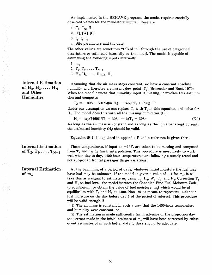
Internal Estimation of H 2, H3, ••• , HN and Other Humidities

Internal Estimation of T2, T3, ••• , TN - 1

Internal Estimation of mo

As implemented in the BEHAVE program, the model requires carefully observed values for the mandatory inputs. These are:

1. TI, TN' HI 2. [T], [W], [C]

3. tp ' t r , ts 4. Site parameters and the date.

The other values are sometimes "talked in" through the use of categorical descriptors or estimated internally by the model. The model is capable of estimating the following inputs internally

1. mo

2. T2, T3,···, TN- I 3. H2, H3, ••• , HN-l' HN.

Assuming that the air mass stays constant, we have a constant absolute humidity and therefore a constant dew point (T d) (Schroeder and Buck 1970). When the model detects that humidity input is missing, it invokes this assump­tion and computes

Td = -398 - 7469/((ln Hi) - 7469/(Ti + 398)) of.

Under our assumption we can replace TI with T2 in this equation, and solve for H2. The model does this with all the missing humidities (Hi):

Hi = exp(7469(1I(Tj + 398)) - lI(Td + 398)). (E-1)

As long as the air mass is constant and as long as the Ti value is kept current, the estimated humidity (Hi) should be valid.

Equation (E-1) is explained in appendix F and a reference is given there.

These temperatures, if input as -1°F, are taken to be missing and computed from T 1 and TN by linear interpolation. This procedure is most likely to work well when day-to-day, 1400-hour temperatures are following a steady trend and not subject to frontal passages (large variations).

At the beginning of a period of days, whatever initial moisture the fuel may have had may be unknown. If the model is given a value of -1 for mo' it will take this as a signal to estimate mo using T l' HI' WI' CI' and Ro. Correcting T 1

and HI to fuel level, the model iterates the Canadian Fine Fuel Moisture Code to equilibrium, to obtain the value of fuel moisture (mo) which would be at equilibrium with TI and HI at 1400. Now, mo is meant to represent 1400-hour fuel moisture on the day before day 1 of the period of interest. This procedure will be valid enough if

(1) The air mass is constant in such a way that the 1400-hour temperature and humidity were constant, or

(2) The estimation is made sufficiently far in advance of the projection day that errors made in the initial estimate of mo will have been corrected by subse­quent estimates of m with better data (3 days should be adequate).

50

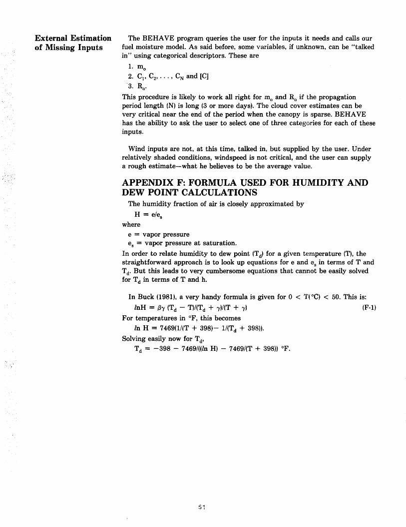
External Estimation of Missing Inputs

The BEHAVE program queries the user for the inputs it needs and calls our fuel moisture model. As said before, some variables, if unknown, can be "talked in" using categorical descriptors. These are

1. mo 2. Cl' C2, ••• , CN and [C)

-3. Ro'

This procedure is likely to work all right for mo and Ro if the propagation period length (N) is long (3 or more days). The cloud cover estimates can be very critical near the end of the period when the canopy is sparse. BEHAVE has the ability to ask the user to select one of three categories for each of these inputs.

Wind inputs are not, at this time, talked in, but supplied by the user. Under relatively shaded conditions, windspeed is not critical, and the user can supply a rough estimate-what he believes to be the average value.

APPENDIX F: FORMULA USED FOR HUMIDITY AND DEW POINT CALCULATIONS

The humidity fraction of air is closely approximated by

H = e/es

where e = vapor pressure es = vapor pressure at saturation.

In order to relate humidity to dew point (T d) for a given temperature (T), the straightforward approach is to look up equations for e and es in terms of T and T d' But this leads to very cumbersome equations that cannot be easily solved for T d in terms of T and h.

In Buck (1981), a very handy formula is given for 0 < T(OC) < 50. This is:

lnH = {3-y (Td - T)/(Td + -y)/(T + -y) (F-1)

For temperatures in of, this becomes

In H = 7469(1/(T + 398)- lI(Td + 398)).

Solving easily now for T d' Td = -398 - 7469/((ln H) - 7469/(T + 398)) of.

51

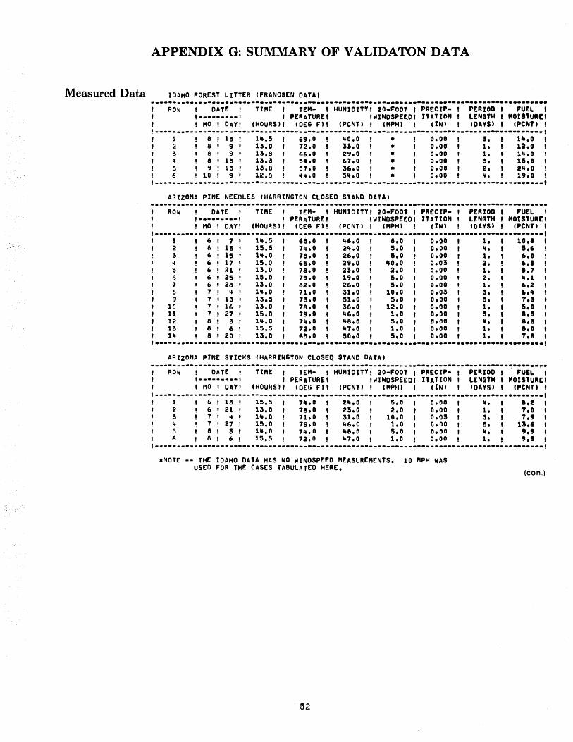
Measured Data

-,:;.'

APPENDIX G: SUMMARY OF VALIDATON DATA

IDAHO FOREST LITTER (FRANDSEN DATA,

---------_.-------.------.---------.---------.-.------------------.. -----.------------.~ ... ROW DATE ,------_._! , MO , DAY!

TIME , TEM- I HUMIDITY' 20-FOOT I PRECIP- , ! PERATURE' IWINDSPEEC' ITATION !

(HOURS" eDEG F" (PCNT) , (MPH' I (IN' ,

PERIOD I FUEL , LENGTH I MOISTURE' (DA'S' I (PC,." I

,--.--~--------------.. --.-----------.--------.-----.-----~-------.-.------.--.~.--.. ~-.-~, 1 8 13 1'+.5 6,.0 '+0.0 • 0.00 311 1".0 2 a , 13.0 72.0 33.0 • 0.00 1. 12.0 3 8 9 13.8 66.0 29.0 • 0.00 1. 1 ... 0 4 8 13 13.3 51t.0 67.0 • O.QO 3. 15.0 5 9 13 13.8 57.0 36.0 • 0.00 2. a ... o 6 10 9 12.6 ..... 0 54.0 ! * 0.00 4. 19.0

,.------_._-----------_._---------------_._.-------------.----.----~.-----~.----.--..... -., ARIZONA PINE NEEDLES (HARRINGTON CLOSED STANO DATA,

--------.---.----------.----~--.---------~ .. ---------.-.-----.-.---.. --.-.-.---.---.. ~ .. -.. ROW DATE I TIME , TEM- I HUMIDITY' 20.FOOT I PRECIP- , PERIOD f FUEL , 1---------, , PERATURE' IWINDSPEED, ITATION , LENGTH , MOISTUREI , MO I DAY! (HOURS' ! eOEGF'! (peNT) I (MPH' cIN' eOA'IS' , (PCNT' ,

!----------------------._.---_ .. _.-----.-.---.-.---._.-------------------·_---···-··_·_--·t 1 6 '7 1'+.5 65.0 ,+6.0 8.0 0.00 1. 10.8 2 " 13 15.5 7'1.0 2,+.0 5.0 0.00 ... 5.' 3 6 15 '''.0 78.0 26.0 5.0 0.00 1. 6.0 .. 6 17 15.0 65.0 29.0 '0.0 0.03 2. 6.! 5 6 21 13.0 78.0 23.0 2.0 0.00 1. 5.7 6 6 25 1!5.1t 79.0 19.0 5.0 0.00 2. •• 1 7 6 28 13.0 82.0 2E,,0 5.0 0.00 1. 6.2 e 7 4 1".0 71.0 31.0 10.0 0.03 3. 6." 9 7 13 13.5 73.0 51.0 5.0 0.00 5. 7.3

10 7 16 13.0 78.0 36.0 12.0 0.00 1. 5.0 11 7 27 15.0 '79.0 "6.0 1.0 0.00 5. I.! 12 8 3 14.0 7 ... 0 48.0 5.0 1'.00 ". 8.1 13 8 6 15.5 72.0 '17.0 1.0 0.00 1. a.o 14 8 20 13.0 65.0 50,0 5.0 0.00 1. 1.8

,.-----------------------------_._-_.-.------._ .. -._.---.------.--.. --.---.-.-~ ..... --.... , ARIZONA PINE STICKS (HARRINGTON CLOSEO STAND DATA'

.. ---------------.----------------.--.----._.-.. -._--.-------.-----~--.-.-.~-.-.-~ ..... -~. ROW ! OATE , TIME , TEM- I HUMIDITYI 20-FOOT , PRECIP- I PERIOD I FUEL , ,---------1 , PERATUREI 'WJNCSPEED' ITATION , LENGTH I .. OISTUREI , no , DAYt (HOURS' I CO[G FI' (peNT' , (MPH' I UN) I tcAyst I (PtNT' ,

-------.--.-----------------~--------.------.. ------.-.-.. --.-..... ----.-....•...•.•. ~.--, 1 6 13 15.5 7 ... 0 2".0 5.0 0.00 ... '.2 2 6 21 13.0 '78.0 2!.0 2.0 0.00 1. ?o 3 7 .. 1'+.0 71.0 31.0 10.0 0.03 3. 7.9 4 7 27 15.0 '79.0 46.0 1.0 0.00 5. sa., 5 8 3 1'+.0 7".0 "8.0 !S.O 0.00 ... •• 9 6 8 (, 15.5 72.0 '+7.0 1.0 0.00 1. 9.1

-----------.-._------.---------------.------.-----.-•• -----.--.-.--~-----•• -----~--.~ •• --! .NOTE -- THE IDAHO DATA HAS NO WINOSPEEO MEASUREMENTS. 10 MPH WAS

USEO FOR THE CASES TABULATED HERE.

52

(eon.)

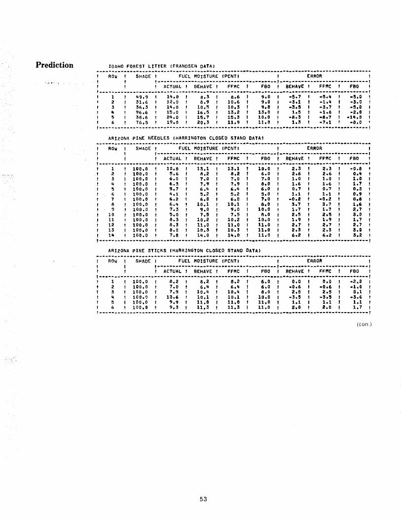
Prediction IDAHO FOREST LITTER (FRANDSEN DATA) ------.---------------------------.-------------.--.------._.--.---_.-.. -----.-----_._----

ROW SHADE , FUEL MOISTURE (peNT' ERROR !---------------------------------------!-----------------------------!

ACTUAL' BEHAVE' FFMC FBO BEHAVE' FFMC FBO !----------------------------------------_ .. ---_.----- -------~-------------------.-------,

1 ~9.9 1~.0 8.3 8.6 9.0 -5.7 -5 ... -5.0 2 31.6 12.0 6.9 10.6 9.0 -3.1 -1 ... ·3.0 3 36.3 1~.0 10.5 10.3 9.0 -3.5 .. 3.7 -!S.O It 96.6 15.0 16.5 13.2 13.0 1.5 -1.8 -2.0 S 38.6 2~.0 15.7 15.3 10.0 -8.3 -8.7 -1_.0 6 76.5 19.0 20.3 11.9 11.0 t.!! -7.1 -0.0

,-----------------------------------------------------··------·····--"··--······-········f ARIZONA PINE NEEOLES (HARRINGTON CLOSED STAND DATA,

-.---------------------------------------------._--.--------.---------------_.------------ROW S~AOE , FUEL MOISTURE (PCNT) ,ERROR ,

,---------------------------------------,-----------------------------, ACTUAL' BEHAVE! FFMC' FBO r BEHAVE! FFMC , FBO !---------_._----------------------------------_.-----------------------------------_._--!

1 100.0 10.8 13.1 13.1 10.0 2.3 2.3 -0.8 l 100.0 5.6 8.2 8.2 6.0 2.6 2.6 0._ 3 100.0 6.0 7.0 7.0 7.0 1.0 1.0 1.0 4 100.0 6.3 7.9 7.9 8.0 1.6 1.6 1.7 5 100.0 5.7 6.~ 6.4 6.0 0.7 0.7 0.3 6 100.0 4.1 5.2 5.2 5.0 1.1 1.1 0.9 7 100.0 6.2 6.0 6.0 7,0 -0.2 -0.2 0,8 8 100.0 6.~ 10.1 10.1 &.0 3.7 3.7 1.6 9 100.0 7.3 9.0 9.0 10.0 1.7 1.7 2.7

10 100.0 5.0 7.5 7.5 8.0 2.5 2.5 3.0 11 100.0 8.3 10.2 10.2 10.0 1.9 1.9 1.7 12 100.0 8.3 11.0 11.0 11.0 2.7 2.7 2.7 13 100.0 8.0 10.3 10~3 11.0 2.3 2.3 3.0 1_ 100.0! 7.8 14.0 1~.0 11.0, 6.2 6.2 3.2

,--------------------------------------------------.-------------------------------------, ARIZONA pINE STICKS (HARRINGTON CLOSED STAND DATA'

ROW SHADE I FUEL MOISTURE (peNT) ,ERROR I

,---------------------------------------,-----------------------------! ACTUAL! BEHAVE I FFMC I FBO I BEHAVE' FFMC , FBO ,

,------------------------------------------~-.----.-.-----------------------·_-----------t 1 2 3 ~ 5 6

100.0 100.0 100.0 100.0 100.0 100.0

6.2 7.0 7.9

13.6 9.9 9.3

8.2 6.'+

10.~ 10.1 11.0 11.3

8.2 6.'+

10.4 10.1 11.0 11.3

6.0 6.0 8.0

10.0 11.0 11.0

0.0 -0.6 2.5

-3.5 1.1 2.0

0.0 -0.6 2.5

-3.5 1.1 2.0

-2.2 .1.0

0.1 -3.6 1.1 1.7

!----------------------------------------------------------------------~-----------------! (con.)

53

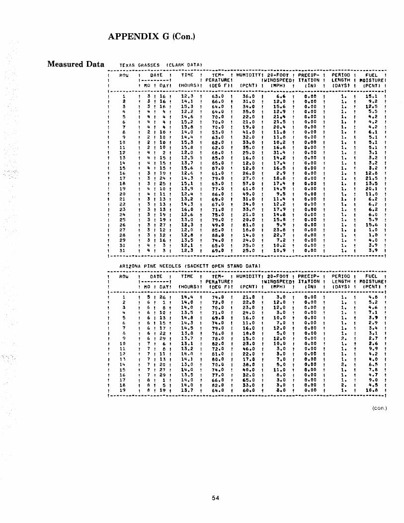
APPENDIX G (Con.)

Measured Data TEXAS GRASSES (CLARK DATA)

-------------~---------------------------------.---------------.---------------------------ROW , OATE I TIME TEM- , HUMIDITY! 20-FOOT ! PRECIP- I PERIOD ! FUEL , 1---------1 I PERATURE! IWINDSPEED! IunON ! LENGTH , PlOISTURE! , , ,,0 ! DAY' (HOt/RS) I (QEG n I ( peNT) I (MPH' ! (IN) I (DAYS' I (peNT) t

,------------------- ------------------------------~------------------.--.----------------! 1 3 , 16 12.3 63.0 36.0 6.6 0.00 1. 15.1 2 3 16 1'+.1 66.0 :51.0 12.0 0.00 1, 9.2 3 3 If, 15.3 6,+.0 3,+.0 15.6 0.00 1. 12.5 '+ 1+ t '+ 12.2 6,+.0 35.0 12.9 0.00 1. 5.5 5 '+ '+ 1'+.6 70.0 22.0 21 ... 0.00 1. ".2 6 '+ '+ 15.2 70.0 21.0 21.5 0.00 1. '+.2 7 '+ '+ 15.8 70.0 19.0 20.,+ 0.00 1. ".2 6 2 10 14.0 53.0 1+1.0 11.8 0.00 I, 6.1 9 2 10 1'+.4 63.0 32.0 11.8 0.00 1. 5.1

10 2 10 15.3 62.0 33.0 10.2 0.00 1. 5.1 11 2 10 15.8 62.0 35.0 16.8 0.00 1. 5.1 12 '+ 2 12.0 68.0 25.0 31.4 0.00 1. 3.1 13 '+ 15 12.5 85.0 16.0 11+.2 0.00 1. 3.2 14 4 15 13.7 65.0 12.0 17.'+ 0.00 1. 3.2 15 4 15 15.6 87.0 12,0 16.5 0.00 1. 3.2 16 3 19 12.6 61.0 26.0 2.9 0.00 1. 12.8 17 3 24 1'+.3 79.0 27.0 18.8 0.00 1. 21.5 18 3 25 15.1 63.0 57.0 17.'+ 0.00 1. 13.5 19 4 10 13.9 71.0 61.0 14.9 0.00 1. 20.1 20 '+ 11 12.'+ 86.0 49.0 9.5 0.00 1.. 11.0 21 3 13 13.2 69.0 31.0 11.4 0.00 1. 6.2 22 3 13 14.3 61.0 34.0 12.2 0.00 1. 6.2 23 3 13 16.0 11.0 33.n 17.9 0.00 1. 6.2 24 3 19 12.6 75.0 21.0 14.8 0.00 1. 6.0 25 3 19 13.0 79.0 20.0 15.8 0·00 1. 5.9 26 3 27 12.3 ~9.0 81.0 9.9 0.00 1. 15.6 27 3 12 12.0 85.0 18.0 23.8 0.00 1. 1.0 28 :5 12 12.8 88.0 14,0 22.7 0.00 1. 1.0 29 3 16 13.5 74.0 2'+.0 7.2 0.00 1. 4.0 30 4 :5 12.1 65.0 25.0 10.2 0.00 1. 3.9 31 4 3 12.3 69.0 25.0 10.9 0.00 1. 3.9

t-------------------------------------------------------~-------.. ----------------------.-, ARIZONA PINE NEEDLES (SACKETT OPEN STANO DATA)

----------.---.-------.------.. ---.-_._--.---------.-----------.-------------------.-------ROW OATE I TIME , TE"'- 1 HUMIDITY, 20-FOOT , PRECIP- I PERIOD , FUEL I

1---------1 ! PERATURE I IWINDSPEEO. ITATION , LENGTH , ~OISTURE' ! MO , DAY! (HOURS) , (OEG n I (peNT) I (MPH) I (IN' I 'OAYS) I (PCNT, ,

,-----------------._--------------------_.------------------------------------------------, 1 5 26 14.4 74.0 21.0 3.0 0.00 1. '+.8 2 6 1 14.0 72.0 22.0 12.0 0.00 1. 5.2 3 6 6 11+.0 70.0 23.0 12.0 0.00 1. 4.6 4 6 10 13.5 71.0 21+.0 3.0 0.00 1. 1.1 5 6 13 14.8 69.0 16.0 10.0 0.00 1. 3.9 6 6 15 14.3 74.0 11.0 7.0 0.00 1. 2.9 7 6 17 1'+.5 79.0 16.0 12.0 0.00 1. 3.1+ 8 6 22 13.8 16.0 18.0 !S.O 0.00 1. 3.1 9 6 29 13.7 78.0 15.0 12.0 0.00 2. 2.7

10 7 6 13.1 82.0 23.0 10.0 0.00 1. 2.6 11 7 a 13.2 72.0 46.0 3.0 0.00 1. 9.9 12 7 11 11+.0 61.0 22.0 :s.o 0.00 1. , .. 2

l' 1 B 14.1 "0.0 17.0 7.0 G.OO 1. 11.0 14 1 20 13.0 70.0 38.0 5.0 0.00 '-. 6.5 15 7 27 lij.O 7,..0 ,,0.0 11.0 0.00 1. 7.8 16 7 29 13.5 17.0 :52.0 8.0 0.00 1. '+.7 17 A 1 14.0 66.0 ft5.0 3.0 0.00 1. 9.0 18 8 5 11+.0 82.0 :53.0 3.0 0.00 2. 4.5 19 6 19 13.1 64.0 60.0 ~.o 0.0.0 1. 10.8

, ____________ - ____ - ____ -4 ___________________________ --------------------------------------t

(con.)

54

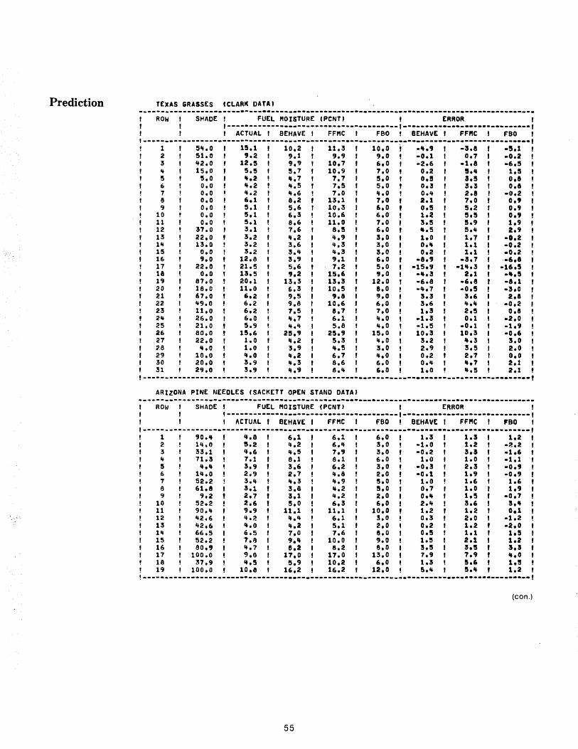
Prediction TEXAS GRASSES CClARK DATA, -.----.---.-------.---.-----------_.-------.-.-----.------._.------------.---------------.

ROW SHADE ! FUEL MOISTURE (peNT) ERROR ,-----._--------------------------------,-------_._._-----------_._._-,

ACTUAL I BEHAVE , FFMC I FBO BEHAVE I FFMC FBO 1----------------------------------------------_·_---------~.---------------------------.,

1 5".0 15.1 10.2 11.3 10.0 • ... 9 -3.8 ·S.l 2 51.0 9.2 9.1 9.9 9.0 ·0.1 0.7 .0.2 3 "2.0 12.5 9.9 10.7 6.0 -2.6 .t.8 -6.5 '+ 15.0 5.5 5.7 10.9 7.0 0.2 5 ... 1.5 5 5.0 ".2 ".7 7.7 5.0 0.5 !.5 0.8 6 0.0 ".2 ... 5 7.5 5.0 0.3 3.3 0.8 7 0.0 '+.2 ".6 7.0 ".0 0 ... 2.8 ·0.2 8 0.0 6.1 8.2 13.1 7.0 2.1 7.0 0.9 9 0.0 5.1 5.6 10.3 6.0 0.5 5.2 0.9

10 0.0 5.1 6.3 10.6 6.0 1.2 5.S 0.9 11 0.0 5.1 8.6 11.0 7.0 3.5 5.9 1.9 12 37.0 3.1 7.6 8.5 6.0 ... 5 5 ... 2.9 13 22.0 3.2 ... 2 ".9 3.0 1.0 1.7 ·0.2 1'+ 13.0 3.2 3.6 ... 3 3.0 0." 1.t ·0.2 15 0.0 3.2 3." ... 3 3.0 0.2 1.1 ·0.2 16 9.0 12.8 3.9 9.1 6.0 -8.9 -3.7 ,·6.8 17 22.0 21.5 5.6 7.2 5.0 ·15.9 -1 ... 3 -16.5 18 0.0 13.5 9.2 15.6 9.0 • ... 3 2.1 .... 5 19 87.0 20.1 13.3 13.3 12.0 -6.8 -6.8 ·a.l 20 18.0 11.0 6.3 10.5 8.0 - ... 7 ·0.5 -3.0 21 67.0 6.2 9.5 9.8 9.0 3.3 3.6 2.8 22 "9.0 6.2 9.8 10.6 6.0 3.6 ..... .0.2 23 11.0 6.2 1.5 8.1 7.0 1.3 2.5 0.8 2 .. 26.0 6.0 ... 1 6.1 ... 0 -I.! 0.1 -2.0 25 21.0 5.9 '+ ... 5.8 ... 0 ·1.5 -0.1 -1.9 26 80.0 lS.6 2S.9 25.9 15.0 10.3 10.3 -0.6 27 22.0 1.0 ".2 5.3 ".0 3.2 '+.3 3.0 '-8 ".0 1.0 3.9 ... 5 3.0 2.9 3.5 2.0 29 10.0 't.o 't.2 6.7 4.0 0.2 2.7 0.0 30 20.0 3.9 4.3 8.6 6.0 0.4 ... 1 2.1 31 29.0 3.9 4.9 8.'+ 6.0 1.0 ".5 2.1

!-----------------------------------------------------------------------------------_.-.-! ARIZONA PINE NEEDLES (SACKETT OPEN STANO DATA)

-------------------------._--------.-----------_.-._-----------------------------------.-. ROW SHADE FUEL MOISTURE (peNT) ERROR

,---------------------------------------1-----------------------------, ACTUAL , BEHAVE , FFMC FBO BEHAVE I FFMC FaD .----.-----------.-------.---._-----------.-.-._-.. --------_ .. _--_ .... _---_._._._. __ ._.-,

1 90." ".8 6.1 6.1 6.0 1.! 1.3 1.2 2 1 ... 0 5.2 ' .. 2 6.4 3.0 -1.0 1.2 .2.2 3 33.1 4.6 ,+.5 7.9 3.0 -0.2 3.3 -1.6 It 71.3 1.1 8.1 8.1 6.0 1.0 1.0 -1.1 5 ... ct 3.9 3.6 6.2 3.0 ·0.3 2.3 -0.9 (, 14.0 2.9 2.7 ... e 2.0 -0.1 1.9 -0.9 7 52.2 3.4 ... 3 '+.9 5.0 1.0 1.6 1.6 a 61.8 3.1 3.8 4.2 5.0 0.7 1.0 1.9 9 9.2 2.7 3.1 ... 2 2.0 0 ... 1.5 .0.1

10 52.2 2.6 5.0 6.3 6.0 2.4 3.6 3." 11 90.4 9.9 11.1 11.1 10.0 1.2 1.2 0.1 12 "2.6 '+.2 ".4 6.1 3.0 0.3 2.0 -1.2 13 "2.6 '+.0 ... 2 !S.1 2.0 0.2 1.2 -2.0 14 66.5 6.5 1.0 1.6 8.0 0.5 1.1 1.5 15 52.2 1.a 9.'+ 10.0 9.0 1.5 2.1 1.2 16 ao., ".7 8.2 8.2 8.0 3.!5 5.5 3.5 17 100.0 9.0 17.0 17.0 13.0 7.9 1.9 ".0 18 ~7.9 ".5 5.9 10.2 6.0 1.3 5.6 1.5 19 100.0 10.8 1&.2 1&.2 12.0 5." 5 ... 1.2

!------------------------------------------------------------------------.... _._---------! (con.)

55

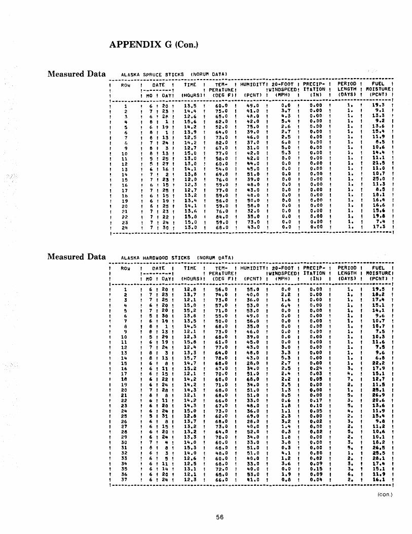
APPENDIX G (Con.)

Measured Data ALASKA SPRUCE STICKS (NaRUM DATA) ----------------------------------------------------------------------------------_._ ... -.-

ROW DATE TIME I TEM- , HUMIDITY' 20-FOOT , PRECIP- I PERIOD , FUEL I

!---------, ! PERATUkE! !WINDSPEED! ITATION I L(NGTH t MOISTURE! , MO , DAYI (HOURS' I (OEG F)' (peNT) I ,PlPH) , (IN' , (DAYS' t (PCNT) , ,. ______ -______________ -- ___________ --._---_____ .. __ --------------------------------------1 1 6 20 13.5 60.0 49.0 0.0 0.00 1. 19.3 2 7 23 11+.4 75.0 41.0 3.7 0.00 1. 9.1 :3 6 2A 12.6 65.0 48.0 4.3 0.00 1. 13.3 4 e 1 15.6 62.0 42.0 5.4 0.00 1. 9.2 5 6 19 14.2 52.0 75.0 2.6 0.00 1. 13.6 (, 8 1 13.9 64.0 39.0 2.7 0.00 1. 15." 7 8 13 12.5 73.0 46.0 2.5 0.00 1. 11.9 (, 7 24 14.2 82.0 37.0 6.8 0.00 1. 8.5 9 e 3 12.7 67.0 31.0 5.0 0.00 1. 10.6

10 e 13 15.0 77.0 42.0 5.3 0.00 1. t".4 11 5 25 13.0 58.0 42.0 0.0 0.00 1. 11.1 12 ~ 21 13.0 60.0 ..... 0 0.0 0.00 1. 21.5 13 (, 16 14.1 S'+.O 45.0 0.0 0.00 1. 11.0 14 7 2 13.8 £9.0 51.0 0.0 0.00 1. 10.7 15 7 23 12.0 7£,.0 39.0 0.0 0.00 1. 25.0 16 6 15 12.3 59.0 48.0 0.0 0.00 1. 11.3 17 7 25 12.7 71.0 ,,3.0 0.0 0.00 1. 8.5 lb 6 15 13.2 59.0 &+8.0 0.0 0.00 1. 18.1 19 6 19 13.4 56.0 50.0 0.0 0.00 1. 16." 20 (, 25 1'+.1 59.0 58.0 0.0 0.00 1. 16.6 21 7 23 13.1; 76.0 32.0 0,0 0.00 1. 1~.6 22- 7 22 l~.O e ... O :5!5.0 0.0 0.00 1. 19.1 23 7 24 15.0 59.0 73.0 0.0 0.00 1. 7 ... 24 7 30 ! 13.0 6e.o 43.0 0.0 0.00 1. 17.!

1 ___________________________ • _______ - ____________ - __ --------------------------------------,

Measured Data ALASKA HARDWOOD STICKS (NORUM OATA' ------------------.---.---------------.------------.-------------------------.--_.-.. ------

ROW DATE TIME I TEM- , HUMIDITY I 20-FOOT I PAECIP- I PERIOD , FUEL I 1------_·_, ! PERATURE! IWINDSPEEof ITATION , LENGTH I PlOISTUAE, ! MO ! OAY' (HOURS l , (OEG F)' (peNT) r (MPH' (IN) r (DAYS' , (PCNT' !

,----------------------------------------------------------------------_._._------_._-----, 1 6 20 12.e 56.0 5!5.0 0.0 0.00 1. 1'.5 2 7 23 13.7 1 ... 0 40.0 2.2 0.00 1. 18.2 3 7 25 12.1 73.0 36.0 1.6 0.00 1. 17." 4 6 20 15.0 57.0 53.0 6.'+ 0.00 1. 15.1 5 7 20 15.2 71.0 53.0 0.0 0.00 1. 1".1 6 !5 30 13.8 55.0 49.0 0.0 0.00 1. 9.6 7 6 1, 13.5 50.0 56.0 0.0 0.00 t. 10.1 8 8 1 14.5 6e.O 3!5.0 0.0 0.00 1. 10.7 9 e 13 12.1 73.0 46.0 0.0 0.00 1. 7.5

10 5 29 12.3 68.0 39.0 0.0 0.00 1. 10.! 11 6 19 15.8 61.0 45.0 0.0 0.00 1. 11.6 12 7 24 12." 77.0 43.0 !.o 0.00 1. '.5 13 8 3 13.3 6".0 48.0 3.3 0.00 1. 9.6 14 8 13 15.1 78.0 43.0 5.! 0.00 1. 6.e 15 6 8 14.7 6e.O 28.0 2.7 0.00 1. 22.2 16 6 11 15.2 67.0 34.0 2.5 0.2~ 3. 11.9 17 6 15 12.1 70.0 51.0 2.4 0.03 ... 15.1 1ft 6 22 14.2 60.0 68.0 2.2 0.08 7. 12.7 19 6 24 14.2 71.0 34.0 2.5 0.00 2. U.5 20 7 28 14.3· , 68.0 51.0 1.3 0.00 1. 25.1 21 8 8 12.1 68.0 51.0 0.5 0.00 5. 26.9 22 6 11 14.2 66.0 33.0 0.6 0.17 3. 20.6 23 6 20 14.3 67.0 48.0 1.8 0.10 5. 13.6 24 6 2ft 15.0 73.0 36.0 1.1 0.05 4. 11.9 25 5 31 12.8 62.0 69.0 2.3 0.00 2. 15 ... 26 6 8 13.7 68.0 28.0 3.2 0.02 3. '.8 27 6 15 13.2 73.0 1+0.0 1.4 0.00 2. 11.2 28 6 20 13.2 64.0 52.0 0.3 0.02 5. 10.6 29 6 24 13.3 70.0 34.0 1.e 0.00 2. 10.1 30 7 .. 14.0 60.0 33.0 3.8 0.00 3. 18.2 31 8 8 15.3 68.0 51.0 0.3 0.00 !5. 26.5 32 6 3 14.0 48.0 51.0 4.1 0.00 1. 25.5 33 6 5 12.6 60.0 40.0 1.2 0.02 2. 28.1 34 6 11 12.5 68.0 33.0 3.6 0.09 , 3. 17.ft 35 6 14 13.1 72.0 40.0 0.0 0.15 , 3. 15.1 36 6 20 12.1 65.0 53.0 1.9 0.09 I 6. 11.9 37 6 24 12.3 66.0 "1.0 0.8 0.0" , 2. 16.1

!-.-----------------------------------------_._---------------------------------------.... ! (con.)

56

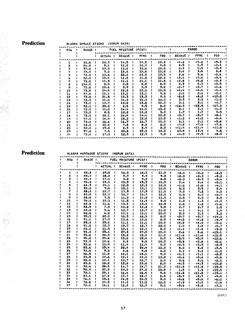
Prediction ALASKA SPRUCE STICKS (NORUM DATA) ----;~~------;~A~~-!-------F~E~-~~is;~RE-~PC~;;------------;---------ERROR---------------,

,--.. --------------------_·-------------t.------------·_---_·_·-------1 , , , ACTUAL r BEHAVE I FFMC r FBO, BEHAVE I FFMC I FDO , ,._--------------------------------------------*---.----_._--------------------._--_.-.. _, I 1 ! ~1.0 f 19.3 ! 1~.5 r 1~.5 , 10.0 r -~.e , -~.e , -9.3 , ,2 8~.0 I 9.1 10.0, 10.0 r 9.0 r 0.9, 0.9 r -0.1 '3 97.0' 13.3 13.6 I 13.6 I 10.0, 0.3 I 0.3' -3.3 ,4 73.0 9.2 12.6, 12.6 10.0! 3.~' 3.~' ole ,5 73.0 13.6 23.2 I 23.2 13.0, 9.6' 9.6 -0.6

(, 52.0 15.4 11.8, 11.8 10.0, -3.6 I -3.6 -5.~ 7 73.0 11.9 11.1 r 11.1 11.0, -0.8 r -o.e -0.9 8 100.0 8.5 8.8, 8.8 8.0! D.! r 0.3 -0.5 9 73.0 10.6 9.9 I 9.9 9.0 r -0.7 -0.7 -1.6

10 73.0 14.4 10.0 t 10.0 10.0 I -~.~ -4.~ -~.4 11 97.0 11.1 13.1! 13.1 ~.o, 2.0 2.0 -2.1 12 73.0 21.5 13.3 I 13.3 9.0' -e.2 -8.2 -12.5 13 73.0 11.0 14.3' 1~.3 10.0! 3.3 3.3 -1.0 14 73.0 10.7 13.8, 13.8 10.0, 3.1 3.1 -0.7 15 52.0 25.0 e.5 r 9.5 8.0 I -16.5 -15.5 -17.0 16 73.0 11.3 1~.4' 14.4 10.0, 3.1 3.1 -1.3 17 73.0 8.5 10.2! 10.2 9,0, 1.1 1,7 0.5 18 73.0 18.1 1~.~' 14.4 10.0, -3.7 -3.7 -a.l -19 97.0 16.4 15.2, 15.2 10.0, ·1.2 -1.2 -6.4 20 73.0 16.6 16.1, 16.1 11.0 I 0.1 0.1-5.6 21 43.0 15.6 7.8, e.2 8.0, -7.8 -7.4 -7.6 22 52.0 19.8 8.4! 8.4 8.0, -11.4 -11.4 -11.8 23 97.0 7.4 20.8, 20.8 12.0, 13.~ 13.~ 4.6

, 24 , 73.0 , 17.3 I 12.3 I 12.3 9.0, -4.9 .~., ·a.! ,.------_ ..... _-----------------------... _--------.. -------_.---------.. --------........ -,

Prediction ALASKA HARDWOOD STICKS (NORUM DATA) .. --------... -------------------._----------------._--------.--.--.---._------------------

ROW SHADE , FUEL MOISTURE (peNT) ERROR ,.-_ .. "_ ..............••...•.••.•••••••. , .•........................... , ACTUAL' BEHAVE I FFMC r FBO BEHAVE' ~FMC FBO

!--------------------_._------------------------------------------------------------_._._, 1 8e.8 19.5 16.5 16.5 11.0 -3.0 -3.0 -8.S 2 80.0 18.2 9.9 9.9 9.0 ·-8.3 -8.3 .9.2 3 eo.o 17.~ 9.2 9.2 a.o -8.3 -8.3 -9.~ ~ 96.3 15.1 15.5 15.5 10,0 o.~ o.~ -5.1 5 66.3 1~.1 12.5 12.5 10.0 -1.6 -1.6 -4.1 6 ge.8 9.6 15.1 15.1 10.0 5.5 5.5 o.~ 7 88.8 10.7 17.9 17.9 11.0 7.2 7.2 0.3 8 80.0 10.7 10.7 10.7 10.0 0.0 0.0 -0,7 9 88.8 7.5 11.0 11.0 11.0 3.5 3.5 3.5

10 9s.8 10.3 11.5 11.5 9.0 1.3 1.3 -1.3 11 ee.8 11.6 13.~ 13.4 10.0 1.8 1.8 -1.6 12 e8.8 1.5 10.2 10.2 9.0 2.7 2.7 1.5 13 a8.8 9.6 13.7 13.7 11.0 4.1 4.1 1.~ 1~ 88.8 6.8 10.1 10.1 10.0 3.3 3.3 3.2 15 99.3 22.2 18.5 18.5 8.0 -3.7 -3.7 -14.2 16 91.5 17.9 13.6 13.6 8.0 -~.3 -~.3 -9.9 17 89.3 15.1 11.1 11.1 10.0 -4.0 -4.0 -5.1 18 91.5 12.7 13.7 13.7 12.0 1.0 1.0 -0.7 19 88.0 11.5 10.1 10.1 8.0 -1.~ -1.4 -3.5 20 93.3 25.1 21.8 27.8 10.0 2.6 2.6 -15.1 21 95.8 26.9 15.2 15.2 11.0-11.6 -11.6 -15.9 22 9_.3 20.6 15.6 15.6 8.0 -5.0 -5.0 -12.6 23 93.9 13.6 9.8 9.8 10.0 -3.8 -~.8 -3.6 2~ '3.8 11.9 11.~ 11.4 e.O -0.5 -0.5 -3.' 25 93.6 15.~ 20.~ 20.~ 12.0 5.0 5.0 -3.4 26 93.5 9.8 9.8 9.8 e.o 0.1 0,1 -1.8 27 86.9 11.2 10.1 10.1 9.0 -1.1 -1.1 ·-2.2 28 e9.9 10.6 10.1 10.1 10.0 -0.6 .0.6 .0.6 2~ 88.0 10.1 10.7 10.7 S.O 0.6 0.6 -2.1 30 89.& 18.2 13.8 13.8 8.0 -4.3 -~.! -10.2 31 93.~ 26.5 14.7 14.7 11.0 -11.8 -11.8 -15.5 32 9&.3 25.5 27~0 21.0 10.0 1.5 1.5 -15.5 33 78.1 28.1 16.~ 16.4 9.0 -11.8 -11.8 -19.1 3~ 83.1 17.~ 13.7 13.7 8.0 -3.1 -3.7 -9.4 35 16.1 15.1 1_.5 1_.5 9,0 -0.6 -0.6 -6.1 36 75.8 11.9 11.0 11.0 10.0 -1.0 -1.0 -1.9 37 72.0 16.1 12.3 12.3 9.0 -a.e -3.e -7.1

1---·-----------------------------._------------------------_--_. __ ._. __ .... ____ . ___ ... __ , (con.)

57

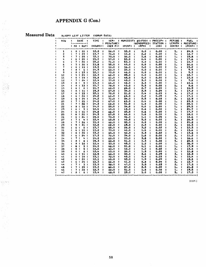
APPENDIX G (Con.)

Measured Data ALASKA LEAF LITTER (NORUM DATA' ------------------.--------------------------------------------._-----._-----.-----.---_.-.

ROW DATE TIME , TEM- , HUMIDITY' 20-FOOT , PRECIP. , PERIOD , FUEL , ~---------!

, PERATURE' !WtNDSPEED, ITATION ! LENGTH , MOISTURE! ! MO I DAY' (HOURS) , (DEG F" (peNT' f (MPH) (IN' , (DAYS' ! (PCNT' !

!---------------------------------_.---------------------------------------------------_._! 1 6 20 12.8 56.0 55.0 0.0 0.00 1. 2".5 2 7 23 13.7 71t.O "0.0 2.2 0.00 1. 12.7 :3 7 25 12.1 73.0 36.0 1.6 0.00 1. IS.8 .. 6 20 15.0 57.0 53.0 6." 0.00 1. 17.6 5 7 20 15.2 71.0 53.0 0.0 0.00 1. 10.7 6 5 30 13.8 55.0 '+9.0 0.0 0.00 1. 16.6 7 6 19 13.5 50.0 56.0 0.0 0.00 1. 15.2 e e 1 lIt.S 68.0 35.0 0.0 0.00 1. 9.9 I) 8 13 12.1 73.0 '+6.0 0.0 0.00 1. 9.3

10 5 29 12.3 68.0 39.0 0.0 0.00 1. 12.7 11 6 19 15.8 61.0 "S.O 0.0 0.00 1. 10.0 12 7 24 12.'+ 77.0 '+3.0 3.0 0.00 1. 7.2 13 e 3 13.3 6 ... 0 '+8.0 3.3 0.00 1. 10.6 14 8 13 15.7 78.0 '+3.0 5.3 0.00 1. 8.6 15 6 A 1".7 68.0 28.0 2.7 0.00 1. 1".9 16 ,; 11 15.2 67.0 3'+.0 2.S 0.2'+ 3. 11.2 17 6 ~5 12.1 70.0 51.0 2.'+ 0.03 ... 17.2 18 6 22 1".2 60.0 68.0 2.2 0.05 7. 17.1 19 6 2'+ 1'+.2 71.0 3'+.0 2.5 0.00 2. 12.9 20 7 25 1'+.8 67.0 63.0 0.'+ 0.00 1. 23.3 21 7 28 1'+.3 68.0 51.0 1.3 0.00 1. 28." 22 8 18 1'+.0 S9.0 3 ... 0 0.0 0.00 1. 29.5 23 6 3 12." '+9.0 '+3.0 0.8 0.00 1. 2".1 24 6 11 1".2 66.0 33.0 0.6 0,00 1. 11.1 2S 6 20 14.3 61.0 "8.0 1.8 0.10 5. 18.0 26 6 24 15.0 73.0 36.0 1.1 0.05 ... 12.6 27 7 .. 12." 60.0 40.0 5.0 0.00 3. 26.9 28 7 28 15.0 68.0 55.0 0.0 0.00 1. 21.2 29 5 31 12.8 62.0 69.0 2.3 0.00 2. 16.3 30 6 8 13.7 68.0 28.0 3.2 0.02 3. 12.3 31 6 15 13.2 73.0 ,,0.0 1.4 0.00 2. 13.6 32 6 20 13.2 64.0 52.0 0.3 0.02 5. 13.6 33 6 24 13.3 70.0 34.0 1.8 0.00 2. 11.2 34 7 .. 1'+.0 60.0 33.0 3.8 0.00 3. 16.6 35 e 8 lS.3 68.0 51.0 0.3 0.00 5. 20.5 36 8 18 12.4 53.0 45.0 1.2 0.00 1. 26.9 37 6 3 1".0 48.0 51.0 4.1 0.00 1. 17.9 38 6 5 12.6 60.0 40.0 1.2 0.02 2. 13.4 39 6 8 12.4 63.0 30.0 1.3 0.00 1. t2.' .. 0 6 11 12.5 68.0 33.0 3.6 0.09 3. 12.3 41 6 14 13.1 72.0 "0.0 0.0 0.15 3. 10." 42 6 20 12.1 65.0 S3.0 1.9 0.09 6. 12.1 .. ~ 6 2 .. 12.3 66.0 41.0 0.8 0.04 2. 12.1 44 7 3 13.9 58.0 47.0 3.5 O.O! 2. 11.3 45 7 25 13.3 68.0 57.0 2.5 O.OG 1. 21,1 46 7 28 12.3 68.0 51.0 1.8 0.00 1. 19.5 47 6 a 13.4 68.0 5'.0 1.0 0.00 S. 17.3

!---------------------------------------------------------------------------------_.------, (con.)

58

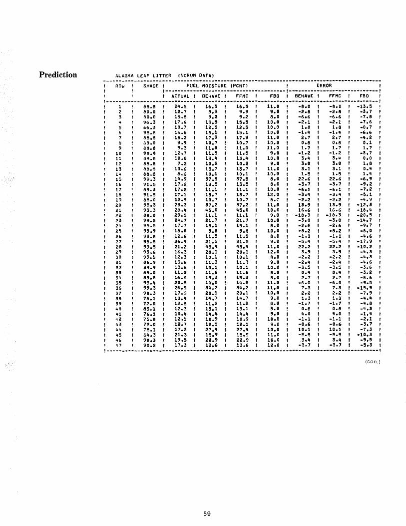
Prediction ALASKA LEAF LITTER (NaRUM DATA) __________ . _________________________ - __________________________ .e_. ______ • ___ • _____ . ______

ROW SHADE I FUEL MOISTURE (PCNT) ERROR !---------------------------------------!----------------------_._.---,

ACTUAL I BEHAVE I FFHC FBO BEHAVE , FFHC FBO !------------------------------------._-------------------------------_.-----------------,

1 88.8 2'+.5 16.5 16.5 11.0 -e.o -e.o -13.5 2 eo.o 12.7 9.9 9.9 9.0 -2.8 -2.8 -3.7 3 130.0 15.6 9.2 9.2 8.0 -6.6 -6.(, -7.8 4 96.3 17.6 15.5 15.5 10.0 -2.1 .2.1 -7.6 5 66.3 10.7 12.5 12.5 10.0 1.8 1.8 .0.7 6 98.8 16.6 15.1 15.1 10.0 -1.4 -1.4 -6.6 7 86.8 15.2 17.9 17.9 11.0 2.7 2.7 - ... 2 8 80.0 9.9 10.7 10.7 10.0 o.e o.e 0.1 9 813.e 9.3 11.0 11.0 11.0 1.7 1.7 1.7

10 CJ6.8 12.7 11.5 11.5 9.0 -1.2 -1.2 -3.7 11 6~.8 10.0 13." 13.4 10.0 3." ~ ... 0.0 12 ee.s 7.2 10.2 10.2 9.0 3.0 3.0 1.8 13 68.8 10.6 13.7 13.7 11.0 3.1 3.1 0.4 14 se.s 8.6 10.1 10.1 10.0 1.5 1.5 1.4 15 99.3 14.9 37.5 37.5 s.o 22.6 22.6 -6.9 16 91.5 17.2 13.5 13.5 8.0 -3.7 -3.7 -9.2 17 89.3 17.2 11.1 11.1 10.0 -6.1 -6.1 -7.2 18 91.5 17.1 13.7 13.7 12.0 -:5.,+ -3.,+ -5.1 19 88.0 12.9 10.1 10.7 8.(' -2.2 -2.2 -4.9 20 93.3 23.3 ~7.2 37.2 11.0 13.9 13.9 -12.3 21 93.3 28.4 '+5.0 4S.0 10.0 1~.~ 16.6 -18.4 22 88.0 29.5 11.1 11.1 9.0 -18.3 -18.3 -20.5 23 99.5 24.1 21.7 21.7 10.0 -3.0 -3.0 -n.7 24 95.5 17.7 15.1 15.1 8.0 -2.1, -2.6 -(Je 7 25 93.9 18.0 '.8 9.8 10.0 -8.2 -8.2 -8.0 26 93.8 12.6 11.5 11.5 8.0 -1.1 -1.1 -4.6 27 95.5 26.9 21.5 21.5 9.0 -5.4 -5.,+ -17.9 28 99.5 21.2 '+3.'+ 43.4 11.0 22.2 22.2 -10.2 29 93.6 16.3 20.1 20.1 12.0 3.9 3.9 -4.3 30 93.5 12.3 10.1 10.1 8.0 -2.2 -2.2 -4.3 31 86.9 13.6 11.3 11. ~ 9.0 -2.'f -2.'f -4.6 32 89.9 13.6 10.1 10.1 10.0 -3.5 -3.5 -3.6 33 a8.0 11.2 11.6 11.6 8.0 0.4 0.4 -3.2 34 89.8 16.6 19.3 19.3 8.0 2.1 2.7 -8.6 35 93.4 20.5 14.5 1'f.5 11.0 -6.0 -6.0 -9.5 36 99.3 26.9 34.2 34.2 11.0 7.3 7.3 ·15.9 37 96.3 11.9 20.1 20.1 10.0 2.2 2.2 -7.9 38 7e.l 13.'f 14.7 1,+.7 9.0 1.3 1.3 -'+.4 39 72.0 12.8 11.2 11.2 8.0 -1.7 -1.1 - ... 8 40 83.1 12.3 13.1 13.1 8.0 o.e 0.8 -4.3 41 76.1 10.4 14.4 1'+.1+ '.0 4.0 4.0 -1.4 42 75.8 12.1 10.9 10.9 10.0 -1.1 -1.1 -2.1 43 72.0 12.7 12.1 12.1 9.0 -0.6 -0.6 -3.1 44 78.1 17.3 27.4 27.4 10.0 10.1 10.1 -7.3 4S 84.3 21.3 15.9 15.9 11.0 -5.5 -5.5 -10.3 '1-6 98.3 19.5 22.' 22.9 10.0 3.,+ 3.4 -'.5 47 90.2 17.3 13.6 13.6 12.0 ';'3.7 -3.7 -5.3

!---------------------------------_.-----------------------------------------------------! (con.)

59

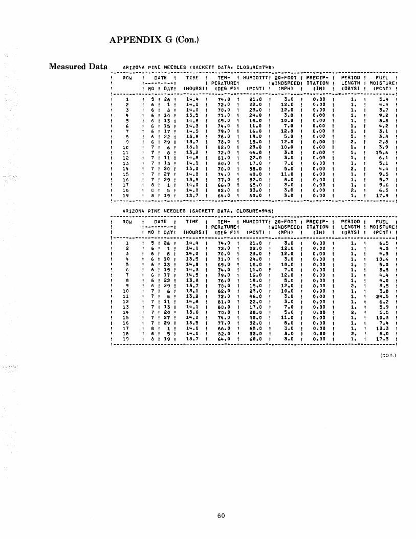
APPENDIX G (Con.)

Measured Data ARIZONA PINE NEEDLES (SACKETT DATA, CLOSURE=7~~'

-.----.--------------------------------------------.------------------.. -------------------ROW DATE TIME , TEM- I HUMIDITY I iO-FOOT I PRECIP- ! PERIOD , FUEL I

!---------I , PERATURE I IWINDSPEEDI nATION ! LENGTH , MOISTURE! ! MO , DAY! (HOURS)I (DEG Ftl (PCNT) ! (MPH' , (IN' (DAYS) ! 'PCNT) !

!-----------------------------------------------------------------------------------------! 1 5 26 lQ.q 7~.0 21.0 3.0 0.00 1. 5." 2 6 1 1'+.0 72.0 22.0 12.0 0.00 1. '+.4 3 6 8 14.0 70.0 23.0 12.0 0.00 1. 3.7 .. 6 10 13.~ 71.0 2'+.0 3.0 0.00 1. 9.2 5 6 13 14.8 69.0 16.0 10.0 0.00 1. 3.8 6 6 15 14.3 7Q.0 11.0 7.0 0.00 1. '+.2 7 6 17 1Q.5 79.0 16.0 12.0 0.00 1. 3.1 a 6 ! 22 13.8 76.0 lS.0 5.0 0.00 1. 3.8 9 6 29 13.7 7e.O 15.0 12.0 0.00 2. 2.e

10 7 6 13.1 82.0 23.0 10.0 0.00 1. 3.9 11 1 8 13.2 72.0 46.0 3.0 0.00 1. 15.6 12 7 11 1~.8 81.0 22.0 3.0 0.00 1. 6.1 13 7 13 14.1 80.0 17.0 7.0 0.00 1. S .1 14 7 20 13.0 70.0 38.0 5.0 0.00 2. '+.,+ 15 7 27 14.0 7,+.0 ~O.O 11.0 0.00 1. 9.5 11l. 7 29 13.5 77.0 32.0 8.0 0.00 1. 5.7 17 8 1 14.0 66.0 65.0 3.0 0.00 1. 9.6 18 e. 5 1'+.0 82.0 33.0 3.0 0.00 2. 6.5 19 8 19 13.7 61+.0 60.0 3.0 0.00 1. 17.9

!-----------------------------------------------------------------------------------------! ARIZONA PINE NEEDLES (SACKETT DATA, CLOSURE=91f",

ROw ! DATE , TIME , TEM- I HUMIDITY, 20-FOOT , PRECIP- I PERIOD I FUEL , !---------! , PERATURE I IWINDSPEEDI ITATION I LENGTH I MOISTUREI

I ! MO 'DAY! (HOURS)' (DEG Fl! (PCNT) I (MPH) ! (IN) I 'DAYS' I (peNT)!

1-----------------------------------------------------------------------------------------, 1 5 ! 26 I 1'+.'+ I 74.0 I 21.0 I 3.0 I 0.00 I 1. I 6.5! 2 6 1 1'+.0 72.0 22.0 12.0 0.00 1. I 4.5 3 6 e 1'+.0 70.0 23.0 12.0 0.00 1. I 4.3 ~ 6 10 13.5 71.0 24.0 3.0 0.00 1. I 10.6 5 6 13 1~.8 69.0 16.0 10.0 0.00 1.! 5.0 6 6 15 llf.3 1,+.0 11.0 7.0 0.00 1. I ~.8 7 6 17 14.5 79.0 16.0 12.0 0.00 1. 4.~ 6 6 22 13.8 76.0 18.0 5.0 0.00 1. 4.0 9 6 29 13.7 78.0 15.0 12.0 0.00 2. 3.5

10 7 6 13.1 82.0 23.0 10.0 0.00 1. 3.8 11 7 8 13.2 72.0 ~6.0 3.0 0.00 1. 21f.S 12 7 11 14.8 81.0 22.0 3.0 0.00 1. 6.2 13 7 13 llf.l 80.0 17.0 7.0 0.00 1. 5.9 14 7 20 13.0 70.0 38.0 5.0 0.00 2. 5.5 15 7 21 14.0 11f.0 '+0.0 11.0 0.00 1. 10.3 16 7 29 13.5 77.0 32.0 8.0 0.00 1. 7.'+ 11 6 1 14.0 66.0 65.0 3.0 0.00 1. 13.3 18 e 5 14.0 82.0 3~.0 3.0 0.00 2. 6.0 19 8 19 13.7 6,+.0 60.0 3.0 0.00 1. 17.3

!-----------------------------------------------------------------------------------------, (con.)

. :,-.1:'

60

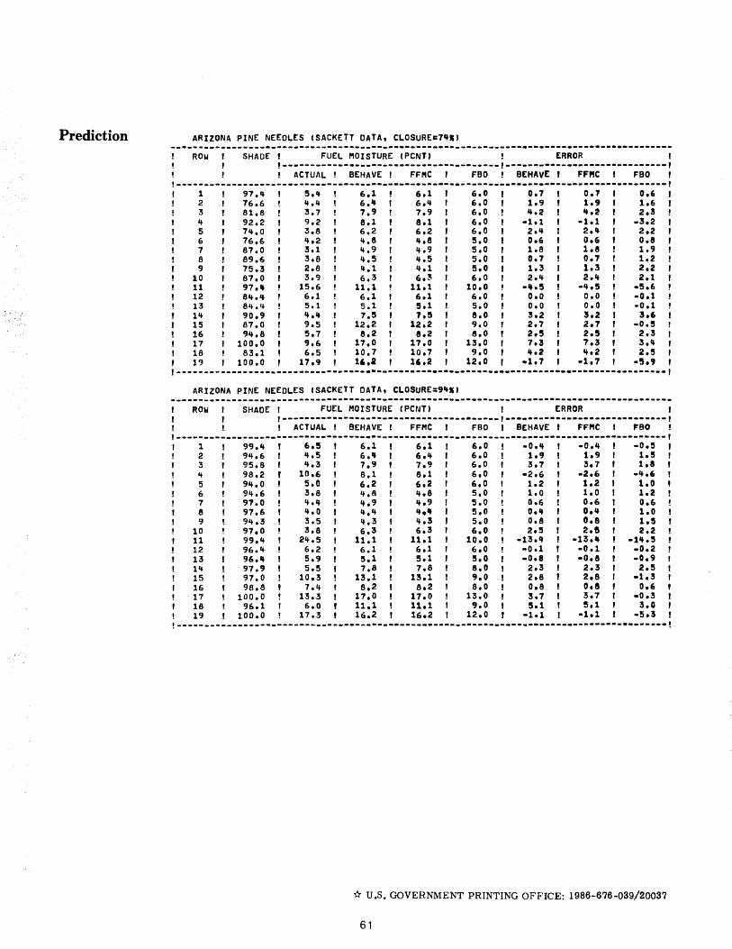
Prediction ARIZONA PINE NEEDL£S (SACKETT DATA. CLOSURE=7~.)

-.-.--------------.--------------------------------.--------------.----.-----.--_.--------ROw SHADE , FUEL fIIOISTURE (PCNT) ERROR ,

,---------------------------------------,-----------------------------, , ACTUAL I BEHAVE ! FFMC , FBO , BEHAVE , FF"C , FBO , !-------------------------------------------_._----_.------------------------------------,

1 97." 5 ... 6.1 6.1 6.0 0.7 0.7 0.6 2 76.6 &t." 6.4 6.&t 6.0 1.9 1.9 1.6 3 81.8 3.7 7.9 7.9 6.0 4.2 4.2 2.5

" 92.2 9.2 e.l 8.1 6.0 -1.1 -1.1 .3.2 5 7&t.O 3.8 6.2 6.2 6.0 2.'t 2." 2.2 6 76.6 4.2 ,+.8 '+.8 5.0 0.6 0.6 0.8 7 87.0 3.1 ,+.9 ... 9 5.0 1.8 1.8 1.9 e 89.6 3.6 '+.5 't.5 5.0 0.7 0.1 1.2 9 75.3 2.8 ,+.1 't.l 5.0 1.3 1.3 2.2

10 87.0 3.9 6.3 6.~ 6.0 2.,+ 2.'+ 2.1 11 97.4 15.6 11.1 11.1 10.0 -It.!5 -'t.5 .5.6 12 a ... 't 6.1 6.1 6.1 6.0 0.0 0.0 ·0.1 13 e".~ 5.1 5.1 5.1 5.0 0.0 0.0 -0.1 1'+ 90.9 ..... 7.5 1.5 8.0 3.2 3.2 3.6 15 87.0 9.5 12.2 12.2 9.0 2.7 2.7 -0.5 16 94.8 5.7 8.2 8.2 8.0 2.5 2.5 2.3 17 100.0 9.6 17.0 17.0 13.0 7.3 7.3 3.4 18 83.1 6.5 10.7 10.7 9.0 't.2 4.2 2.5 19 100.0 17.9 16.2 16.2 12.0 .1.7 -1.7 .S.9

1------------------------------------------·---·----------------------.. -----------------, ARIZONA PINE NEEDLES (SACKETT DATAt CLOSURE=94",

--------~.--------------------------------------------------------.-----------------------ROW SHADE I FUEL MOISTURE (PCNT, ERROR , !---------------------------------------!-----------------------------!

! , ACTUAL' BEHAVE 1 FFMC 1 FBO, BEHAVE I FFMC , FBO !

1----------------------------------------------------------------------------------------1 I 1 I 99.'" 6.5, 6.1, 6.1 I 6.0 -0..., -0... , -o.s I 2 94.6!'" 5 I 6. It, 6.4 I 6. a 1 • ., 1.9' 1.5, :3 95.8 f ".3' 7.9, 7.9 1 6.0 3.7 3.7 I 1.8, .. 98.2' 10.6, 8.1 I 8.1 I 6.0 -2.6 -2.6' -4.6 , 5 94.0' 5.0, 6.2 I 6.2' 6.0 1.2 1.2' 1.0' 6 94.6 3.8 f 4.8 4.8 I 5.0 1.0 1.0 I 1.2 7 91.0 ..... 4.9 4.9 I 5.0 0.6 0.6 I 0.6 e 97.6 ".0 4." 't." 5.0 0.4 o.'t, 1.0 9 94.3 3.5 ... 3 4.3' 5.0 0.8 0.8' 1.5

10 97.0 3.8 6.3 6.3! 6.0 2.5 2.5, 2.2 11 99.4 24.5 11.1 11.1! 10.0 -13.4 -13.4, -14.5 12 96.'+ 6.2 6.1 6.1' 6.0 -0.1 -0.1, .0.2 13 96.4 5.9 5.1 5.1 1 5.0 -0.8 -0.8 I -0.9 14 97.9 5.5 7.8 7.8 I a.o 2.3 2.3 I 2.5 15 97.0 10.3 13.1 13.1 I 9.0 2.6 2.6 I -1.3 16 98.8 7.4 8.2 8.2' 8.0 0.8 0.8 I 0.' 17 100.0 13.3 17.0 17.0 I 13.0 3.7 3.7' -0.3 18 96.1 6.0 11.1 11.1' 9.0 5.1 5.1' 3.0 19 100.0 17.3 16.2 16.2' 12.0 -1.1 -1.1, -5.3

!------------_._------------------------_.--------------------------------------._-------! :.--.

* u.s. GOVERNMENT PRINTING OFFICE: 1986-676-039/20037

61

Rothermel, Richard C.; Wilson, Ralph A.; Morris, Glen A.; Sackett, Stephen S. Modeling moisture content of fine dead wildland fuels: input to the BEHAVE fire prediction system. Research Paper INT-359. Ogden, UT: U.S. Department of Agriculture, Forest Service, Intermountain Research Station; 1986 61 p.

Describes a model for predicting moisture content of fine fuels for use with the BEHAVE fire behavior and fuel modeling system. The model is intended to meet the need for more accurate predictions of fine fuel moisture, particularly in northern conifer stands and on days following rain. The model is based on the Canadian Fine Fuel Moisture Code (FFMC), modified to account for solar heating of fuels and to predict diurnal trends in fine fuel moisture. The model may be initiated without extensive data on prior weather. When compared to the FFMC and the fire behavior officers' procedures, the new model gave consis­tently better predictions over the complete range of fuel conditions.

KEYWORDS: fuel moisture, fine fuels, model, fire behavior, diurnal, solar, shade

INTERMOUNTAIN RESEARCH STATION

The Intermountain Research Station provides scientific knowl­edge and technology to improve management, protection, and use of the forests and rangelands of the Intermountain West. Research is designed to meet the needs of National Forest managers, Federal and State agencies, industry, academic institutions, public and private organizations, and individuals. Results of research are made available through publications, symposia, workshops, training sessions, and personal contacts.

The Intermountain Research Station territory includes Montana, Idaho, Utah, Nevada, and western Wyoming. Eighty-five percent of the lands in the Station area, about 231 million acres, are classified as forest or rangeland. They include grasslands, deserts, shrub­lands, alpine areas, and forests. They provide fiber for forest in­dustries, minerals and fossil fuels for energy and industrial develop­ment, water for domestic and industrial consumption, forage for livestock and wildlife, and recreation opportunities for millions of visitors.

Several Station units conduct research in additional western States, or have missions that are national or international in scope.

Station laboratories are located in:

Boise, Idaho

Bozeman, Montana (in cooperation with Montana State University)

Logan, Utah (in cooperation with Utah State University)

Missoula, Montana (in cooperation with the University of Montana)

Moscow, Idaho (in cooperation with the University of Idaho)

Ogden, Utah

Provo, Utah (in cooperation with Brigham Young University)

Reno, Nevada (in cooperation with the University of Nevada)