GRADUATE RESEARCH REPORT

ECIV 797: CIVIL ENGINEERING RESEARCH

Submitted by-

Md. Mozahid Hossain PhD student,

Department of Civil Engineering

Advisor-

Dr. PAUL H. ZIEHL, P.E.

Department of Civil Engineering

1

MODELING OF FATIGUE CRACK GROWTH WITH ABAQUS

By Mozahid Hossain

Research Assistant, Department of Civil Engineering, University of South Carolina, Columbia, SC, e-mail: hossaimm@email.sc.edu

Abstract:

Fatigue crack initiation in steel structures is one of the most important considerations

facing the infrastructure community. Purely static loading is rarely observed in structural

components. Almost 80% to 95% of all structural failures occur through a fatigue

mechanism. As a result, fatigue analysis has become an early driver in the product

development processes of a growing number of companies.

The traditional approach for determining the fatigue limit for a structure is to establish the

curves (load versus number of cycles to failure) for the materials in the structure. Such an

approach is still used as a design tool in many cases to predict fatigue resistance of

engineering structures although it is generally conservative and no relationship between the

crack length and the cycle number is available.

The computational process to simulate the slow progressive damage in steel over many

load cycles is simple but numerical fatigue life studies usually involve the response of the

structure subjected to a small fraction of the actual loading history. This response then

might be extrapolated over many load cycles using empirical formulae to predict the

likelihood of crack initiation and propagation.

The direct cyclic analysis capability in ABAQUS/Standard provides a computationally

effective modeling technique to obtain the stabilized response of a structure subjected to

periodic loading and is ideally suited to perform low-cycle fatigue calculations on a large

2

structure. The direct cyclic low-cycle fatigue capability is an extension of the direct cyclic

capability that includes damage accumulation and damage extrapolation. It provides

capabilities to model damage growth in steel structure. In material the cyclic loading leads

to stress reversals and the accumulation of plastic strains, which in turn cause the initiation

and propagation of cracks. The damage initiation and evolution are characterized by the

stabilized accumulated inelastic hysteresis strain energy per cycle. The objective of this

research report is to simulate the fatigue behaviour of structural steel with ABAQUS6.9-2.

Significant performance gains with good accuracy of the direct cyclic low cycle fatigue

capability are clearly demonstrated.

Keywords: Cracks, cyclic loading, Low-cycle fatigue, Abaqus, Cyclic loading Mozahid Hossain is a PhD student in the Department of Civil Engineering at University of South Carolina, Columbia, SC. His research interest includes Self Powered Wireless Sensor Network for Structural Bridge Health Prognosis.

3

TABLE OF CONTENT

ABSTRACT……………………………………………………………………... 1

TABLE OF CONTENT…………………………………………………………. 2

LIST OF FIGURE……………………………………………………………… 4

1.0 FATIGUE ANALYSIS …………………………………………………………. 5

2.0 LOADING ……………………………………………………………………..... 6

3.0 MATERIAL PROPERTIES……………………………………………………... 7

4.0 FATIGUE CRACK GROWTH …...……………………………………………. 9

5.0 MODELING WITH ABAQUS………………………………………………….. 23

6.0 FUTURE STUDY ………………………………….…………………………… 29

7.0 REFERENCES ………………………………….………………………………. 31

4

LIST OF FIGURE

Figure 1 Load: (a) Ramp; (b) Step ………………………………………………. 6

Figure 2 Generic representation of the Stress-Strain curve ……………………… 9

Figure 3 Strain-life relation (Coffin-Manson) …………………………………… 10

Figure 4 Plastic shakedown in direct cycling analysis (ABAQUS Manual) …….. 11

Figure 5 Elastic stiffness degradation as a function of the cycle number………... 11

Figure 6 Fatigue crack growth governed by the Paris law ………………………. 12

Figure 7 Schematic sigmoidal behavior of fatigue crack growth rate versus ∆K .. 14

Figure 8 Schematic mean stress influence on fatigue crack growth rates………... 15

Figure 9 Nomenclature for constant amplitude cycling loading ……………….... 19

Figure 10 Elastic stresses near the crack tip (a<<1) ………………………………. 96

Figure 11 Plastic zone size at the tip of a through-thickness crack ……………….. 20

Figure12 Line contour surrounding a crack tip for J-integral formulation……….. 22

Figure 13 Compact Tension Specimen ………………………………….………… 23

Figure 14 Cycling load ………………………………….………………………… 25

Figure 15 Cycling load ………………………………….………………………… 25

Figure 16 Cycling load ………………………………….………………………… 26

Figure 17 Cycling load………………………………….…………………………. 26

Figure 18 Meshing ………………………………….…………………………….. 27

Figure 19 Von Mises Stress………………………………….…………………….. 27

Figure 20 Piezoelectric sensor ………………………………….…………………. 29

Figure 21 Active and Passive Sensing modes used by piezoelectric materials …... 31

5

1.0 FATIGUE ANALYSIS

Fatigue is failure under a repeated or varying load, never reaching a high enough level to

cause failure in a single application. The fatigue process embraces two basic domains of

cyclic stressing or straining, differing distinctly in character. In each domain, failure occurs

by different physical mechanisms (ABAQUS Manual):

1. Low-cycle fatigue—where significant plastic straining occurs. Low-cycle fatigue

involves large cycles with significant amounts of plastic deformation and relatively

short life. The analytical procedure used to address strain-controlled fatigue is

commonly referred to as the Strain-Life, Crack-Initiation, or Critical Location

approach.

2. High-cycle fatigue—where stresses and strains are largely confined to the elastic

region. High-cycle fatigue is associated with low loads and long life. The Stress-Life

(S-N) or Total Life method is widely used for high-cycle fatigue applications—here the

applied stress is within the elastic range of the material and the number of cycles to

failure is large. While low-cycle fatigue is typically associated with fatigue life between

10 to 100,000 cycles, high-cycle fatigue is associated with life greater than 100,000

cycles.

Fatigue analysis refers to one of three methodologies: local strain or strain life, commonly

referred to as the crack initiation method, which is concerned only with crack initiation (E-

N, or sigma nominal); stress life, commonly referred to as total life (S-N, or nominal

stress); and crack growth or damage tolerance analysis, which is concerned with the

number of cycles until fracture.

6

The method for calculating fatigue life is sometimes called the Five Box Trick, including

material, loading, and geometry inputs, and analysis and results. The three main inputs for

fatigue life analyses are processed using various life estimation tools depending on whether

the analysis is for crack initiation, total life, or crack growth.

2.0 LOADING

Pun (2001) demonstrated that the proper specification of loading variation is extremely

important to achieve an accurate fatigue life prediction. The loading can be defined in

various manners and whether it is time-based, frequency-based or in the form of some sort

of spectra depends on the type of fatigue analysis. When working with finite element

models the loading can be force, pressure, temperature, displacement, or a number of other

types. The time history used in a fatigue calculation must be a representation of the time

variation in the loading applied in the Finite Element Analysis (FEA). For simple cases,

this implies a force-time history corresponding to a time variation in the point loading used

in the FEA. There are a number of different kinds of loading possible, each one requiring a

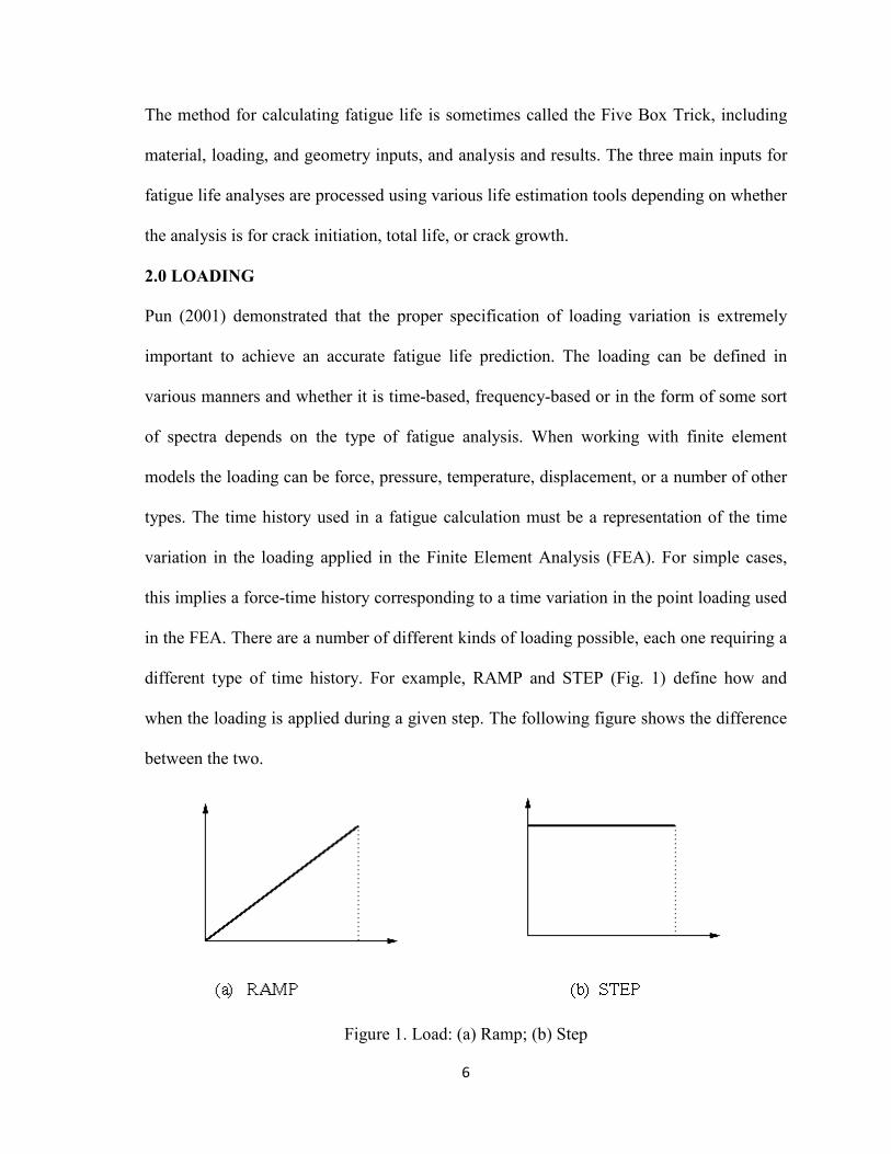
different type of time history. For example, RAMP and STEP (Fig. 1) define how and

when the loading is applied during a given step. The following figure shows the difference

between the two.

Figure 1. Load: (a) Ramp; (b) Step

7

3.0 MATERIAL PROPERTIES

Materials subjected to cyclic loading behave differently than under monotonic loading.

While monotonic material properties are the result of material tests where the load is

steadily increased until a test coupon breaks, cyclic material properties are obtained from

material stress where loading is reversed, then cycled until failure at various load levels.

Different types of cyclic material properties are required depending on the type of fatigue

analysis.

Because it can be difficult to gain access to measured cyclic properties, much effort has

been expended finding ways of relating monotonic properties to cyclic properties. The

approaches have all been empirical but do provide a means of estimating cyclic properties

that are otherwise expensive to generate.

The Ramberg–Osgood equation was created to describe the non linear relationship between

stress and strain—that is, the stress–strain curve—in materials near their yield points. It is

especially useful for metals that harden with plastic deformation (see strain hardening),

showing a smooth elastic-plastic transition.

In its original form, the equation for strain (deformation) is,

)1.........(..........................................................................................n

EK

E

+=

σσε

Where

ε is strain,

σ is stress,

E is Young's modulus, and

K and n are constants that depend on the material being considered.

The first term on the right side,

second term,n

EK

σ , accounts for the plastic part, the parameters

hardening behaviour of the material. Introducing the

defining a new parameter, α, related to

term on the extreme right side as follows:

n

O

On

EEK

=

σ

σσα

σ

Replacing in the first expression, the Ramberg

..........n

O

O

EE

+=

σ

σσα

σε

In the last form of the Ramberg

depends on the material constants

stress and plastic strain, the Ramberg

even for very low levels of stress. Nevertheless, for

commonly used value of the material constants α and n, the plastic strain remains

negligible compared to the elastic strain. On the other hand, for stress levels higher than σ

plastic strain becomes progressively larger

The value EOσα can be seen as a

that EO /)1( σαε += , when

Accordingly (Fig. 2):

Elastic strain at yield

Plastic strain at yield

8

term on the right side, Eσ , is equal to the elastic part of the strain

, accounts for the plastic part, the parameters K and

of the material. Introducing the yield strength of the material, σ

defining a new parameter, α, related to K as1−

=

nO

EK

σα , it is convenient to rewrite the

term on the extreme right side as follows:

................................................................................n

Replacing in the first expression, the Ramberg–Osgood equation can be written as

................................................................................

In the last form of the Ramberg–Osgood model, the hardening behavior

depends on the material constants and . Due to the power-law relationship between

stress and plastic strain, the Ramberg–Osgood model implies that plastic strain is present

even for very low levels of stress. Nevertheless, for low applied stresses and for the

value of the material constants α and n, the plastic strain remains

negligible compared to the elastic strain. On the other hand, for stress levels higher than σ

plastic strain becomes progressively larger than elastic strain.

can be seen as a yield offset, as shown in Fig. 2. This comes from the

when Oσσ = .

lastic strain at yield = EO /σ

lastic strain at yield = )/( EOσα = yield offset

, is equal to the elastic part of the strain. While the

and n describing the

of the material, σ0, and

it is convenient to rewrite the

)2.(....................

Osgood equation can be written as

)3......(....................

hardening behavior of the material

relationship between

Osgood model implies that plastic strain is present

low applied stresses and for the

value of the material constants α and n, the plastic strain remains

negligible compared to the elastic strain. On the other hand, for stress levels higher than σ0,

. This comes from the fact

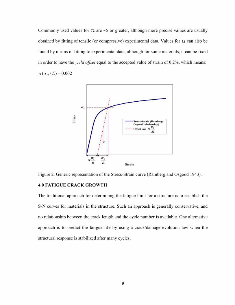
Commonly used values for

obtained by fitting of tensile (or compressive) experimental data. Values for

found by means of fitting to experimental data, although for some materials, it can be fixed

in order to have the yield offset

002.0)/( =EOσα

Figure 2. Generic representation of the Stress

4.0 FATIGUE CRACK GROWTH

The traditional approach for

S-N curves for materials in the structure. Such an approach is generally conservative, and

no relationship between the crack length and the cycle number is available. One alternative

approach is to predict the fatigue

structural response is stabilized after many cycles.

9

Commonly used values for are ~5 or greater, although more precise values are usually

obtained by fitting of tensile (or compressive) experimental data. Values for

found by means of fitting to experimental data, although for some materials, it can be fixed

yield offset equal to the accepted value of strain of 0.2%, which means:

Generic representation of the Stress-Strain curve (Ramberg and Osgood

FATIGUE CRACK GROWTH

The traditional approach for determining the fatigue limit for a structure is to establish the

N curves for materials in the structure. Such an approach is generally conservative, and

between the crack length and the cycle number is available. One alternative

h is to predict the fatigue life by using a crack/damage evolution law when the

structural response is stabilized after many cycles.

are ~5 or greater, although more precise values are usually

obtained by fitting of tensile (or compressive) experimental data. Values for can also be

found by means of fitting to experimental data, although for some materials, it can be fixed

equal to the accepted value of strain of 0.2%, which means:

Osgood 1943).

determining the fatigue limit for a structure is to establish the

N curves for materials in the structure. Such an approach is generally conservative, and

between the crack length and the cycle number is available. One alternative

life by using a crack/damage evolution law when the

10

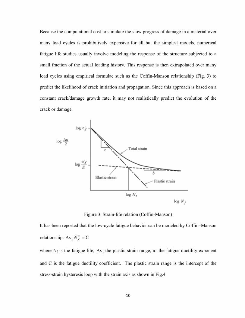
Because the computational cost to simulate the slow progress of damage in a material over

many load cycles is prohibitively expensive for all but the simplest models, numerical

fatigue life studies usually involve modeling the response of the structure subjected to a

small fraction of the actual loading history. This response is then extrapolated over many

load cycles using empirical formulae such as the Coffin-Manson relationship (Fig. 3) to

predict the likelihood of crack initiation and propagation. Since this approach is based on a

constant crack/damage growth rate, it may not realistically predict the evolution of the

crack or damage.

Figure 3. Strain-life relation (Coffin-Manson)

It has been reported that the low-cycle fatigue behavior can be modeled by Coffin–Manson

relationship: CN fp =∆ αε

where Nf is the fatigue life, pε∆ the plastic strain range, α the fatigue ductility exponent

and C is the fatigue ductility coefficient. The plastic strain range is the intercept of the

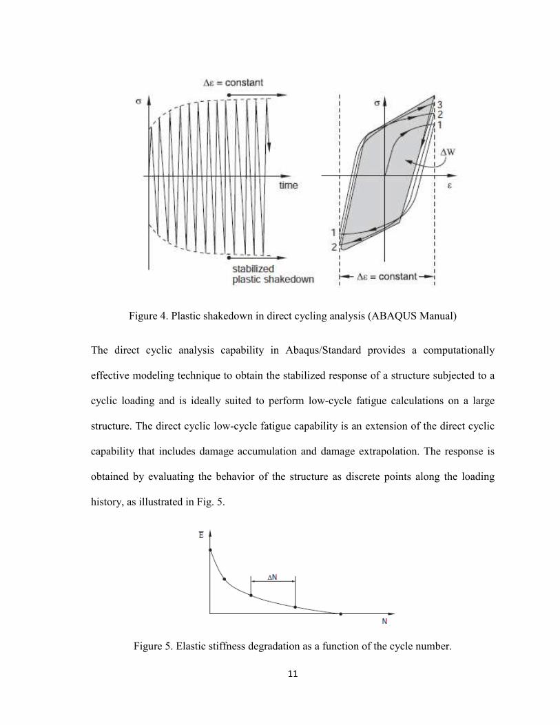
stress-strain hysteresis loop with the strain axis as shown in Fig.4.

11

Figure 4. Plastic shakedown in direct cycling analysis (ABAQUS Manual)

The direct cyclic analysis capability in Abaqus/Standard provides a computationally

effective modeling technique to obtain the stabilized response of a structure subjected to a

cyclic loading and is ideally suited to perform low-cycle fatigue calculations on a large

structure. The direct cyclic low-cycle fatigue capability is an extension of the direct cyclic

capability that includes damage accumulation and damage extrapolation. The response is

obtained by evaluating the behavior of the structure as discrete points along the loading

history, as illustrated in Fig. 5.

Figure 5. Elastic stiffness degradation as a function of the cycle number.

12

The solution at each of these points is used to predict the degradation and evolution of

material properties that will take place during the next increment of load cycles, ∆N. The

degraded material properties are then used to compute the solution at the next point in the

load history. This capability can be used to model progressive damage and failure both in

the bulk material and at the material interface. When failure mechanisms both in the bulk

material and at the interfaces are considered simultaneously, the failure occurs first at the

weakest link in the model. The damage initiation and evolution in the bulk material are

characterized by the accumulated inelastic hysteresis strain energy per stabilized cycle, as

illustrated in Fig. 4.

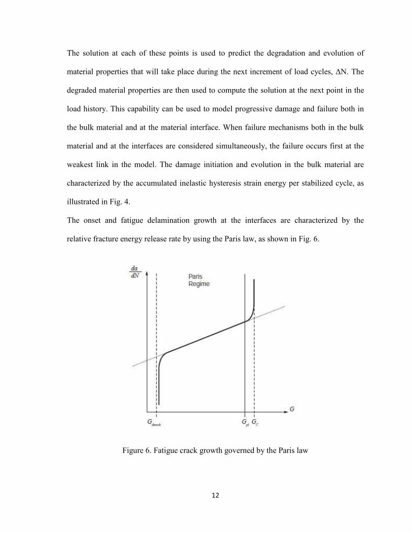
The onset and fatigue delamination growth at the interfaces are characterized by the

relative fracture energy release rate by using the Paris law, as shown in Fig. 6.

Figure 6. Fatigue crack growth governed by the Paris law

13

For linear elastic materials, Griffith’sapproach says that a crack extends if the

thermodynamic crack driving force, characterized by the energy release rate G (Fig. 6),

becomes equal or larger than the crack growth resistance, R (Griffith, 1921), whereas the

Irwin (1957) approach postulates that a crack grows when the crack tip stress intensity

factor K reaches a critical value Kc (Fig. 7). The Griffith and Irwin criteria are equivalent

for linear elastic materials, since energy release rate and stress intensity factor are related.

Crack tip conditions are defined by a single parameter, such as stress intensity factor.

Under cyclic constant amplitude stress intensity, the crack growth rate for small plastic

zones at the crack tip is defined by: ���� � ���� � where,

∆K cycles between Kmax – Kmin

R = Kmin / Kmax=Smin/Smax

da/dN = crack growth rate per cycle, L(cycle)-1

In field-situations, a history dependent factor is added into the function to account for

previous loading conditions during service-life of the element. The similitude assumption

shown for crack growth rate does not take into account occasional overloads and/or under

loads which will turn the problem into a variable amplitude loading configuration. Since

the stress intensity factor cannot characterize excessive plasticity at crack tip, researchers

proposed that crack growth be a function of J-integral. For fatigue resulting in large-scale

yielding, the ∆J value will be employed and is analogous from monotonic loading.

Fatigue crack propagation curve (log da/dN–log ∆K) may be divided into three stages

which are typical for: short crack growth propagation stage (Region I), long crack

propagation (Region II), and fracture stage (Region III) (Fig. 5). Where the behavior of the

14

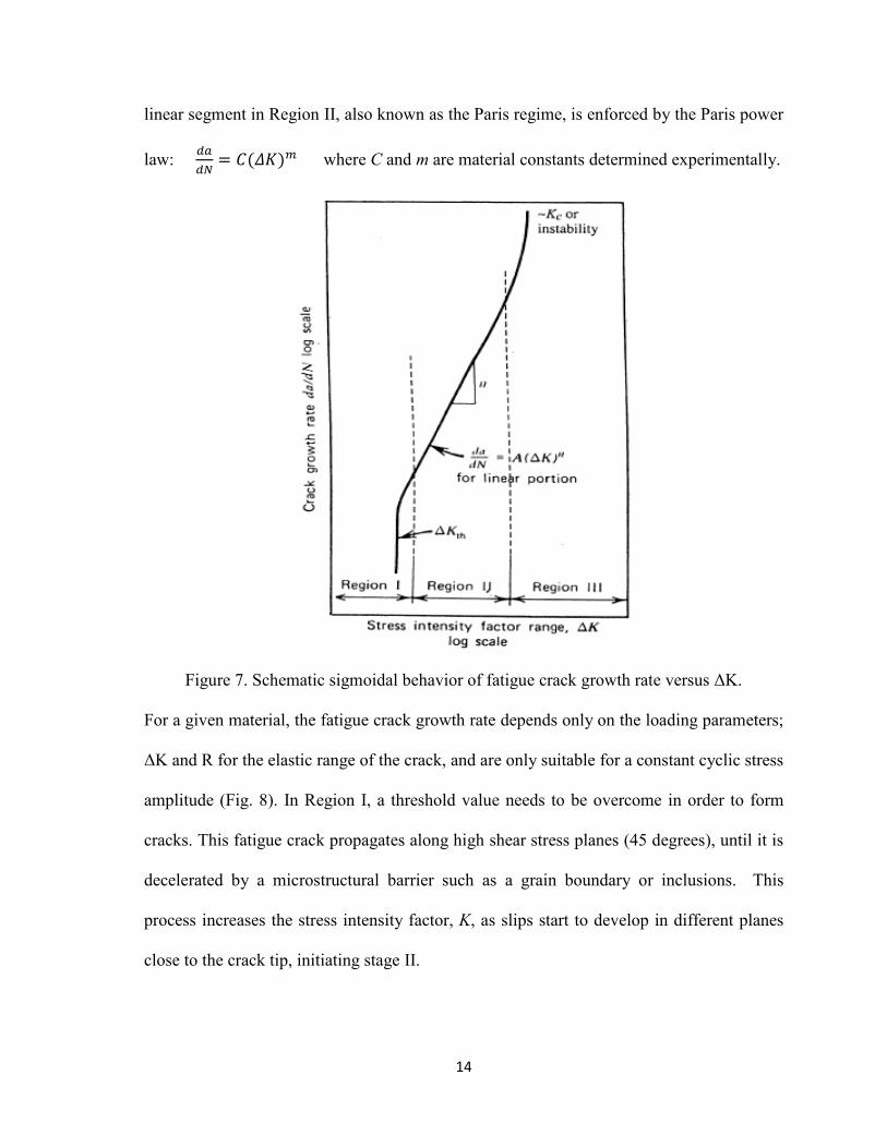
linear segment in Region II, also known as the Paris regime, is enforced by the Paris power

law: ���� � ����� where C and m are material constants determined experimentally.

Figure 7. Schematic sigmoidal behavior of fatigue crack growth rate versus ∆K.

For a given material, the fatigue crack growth rate depends only on the loading parameters;

∆K and R for the elastic range of the crack, and are only suitable for a constant cyclic stress

amplitude (Fig. 8). In Region I, a threshold value needs to be overcome in order to form

cracks. This fatigue crack propagates along high shear stress planes (45 degrees), until it is

decelerated by a microstructural barrier such as a grain boundary or inclusions. This

process increases the stress intensity factor, K, as slips start to develop in different planes

close to the crack tip, initiating stage II.

15

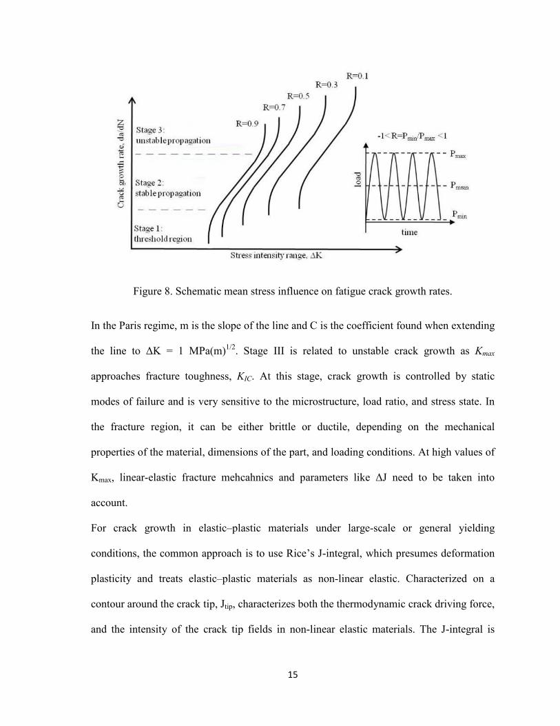
Figure 8. Schematic mean stress influence on fatigue crack growth rates.

In the Paris regime, m is the slope of the line and C is the coefficient found when extending

the line to ∆K = 1 MPa(m)1/2. Stage III is related to unstable crack growth as Kmax

approaches fracture toughness, KIC. At this stage, crack growth is controlled by static

modes of failure and is very sensitive to the microstructure, load ratio, and stress state. In

the fracture region, it can be either brittle or ductile, depending on the mechanical

properties of the material, dimensions of the part, and loading conditions. At high values of

Kmax, linear-elastic fracture mehcahnics and parameters like ∆J need to be taken into

account.

For crack growth in elastic–plastic materials under large-scale or general yielding

conditions, the common approach is to use Rice’s J-integral, which presumes deformation

plasticity and treats elastic–plastic materials as non-linear elastic. Characterized on a

contour around the crack tip, Jtip, characterizes both the thermodynamic crack driving force,

and the intensity of the crack tip fields in non-linear elastic materials. The J-integral is

16

independent of the contour used to evaluate it, so Jtip = Jfar where Jfar is the integral on a

contour in the far-field. This path independence is important, since the energy released at

the crack tip (Jtip) cannot be easily measured, whereas the total energy released during

crack extension in a body (Jfar) can be readily measured.

In homogeneous elastic materials, Jtip is identical to the total energy released in the

specimen per unit crack extension, whereas this is not so in elastic–plastic materials due to

the dissipation in the plastic zone which induces the plasticity influence term, Cp, defined

as the total configurationally force due to plasticity, projected on the crack growth

direction. For deformation plasticity, the plasticity influence term Cp vanishes in the

context of deformation plasticity, whereas the crack driving force Jtip vanishes for rigid

plasticity.

An experimental study on C(T) specimens to examine the influence of plastic deformation

near the crack tip was performed on annealed mild steel with a Young’s modulus of 200

GPa. Loading was simulated by prescribing the load line displacement νll assuming plane

strain conditions. The far-field J-integral values are compared to ABAQUS values

calculated using the virtual crack extension and to experimental values determined from the

area below the load vs. load-line displacement curve (Rice, 1973). Results showed that the

configurational body force arises only due to plastic deformation and is large directly at the

crack tip for homogeneous material. From the calculated plastic zone of 2 mm, the

configurational force rapidly decreases to zero at a distance less than 2 mm. Abaqus

showed that a plastic deformation starts at the back face of the specimen for νll=0.2 mm (a)

and as it increases to 0.343 mm (b) and 0.352 mm (c) show that with increasing loading,

both the crack tip plastic zone and the region of remote plasticity expand. The two regions

17

eventually merge and general yielding ocurrs in the ligament. J-integral Jtip is the scalar

driving force on a crack tip in elastic–plastic materials.

After an extensive analysis performed on the behavior of the J-integral for different cases,

it was concluded that the scalar driving force at the crack tip of an elastic-plastic material is

defined as Jtip. The crack driving force, Jtip, is equal to the sum of the global driving force

Jfar and the plasticity influence term Cp, therefore Jtip = Jfar+Cp. It was also found that the J-

integral is path-independent in homogenous elastic bodies due to the fact that

configurational body forces disappear, but in elastic-plastic bodies these forces are present

and depend on the plastic strain gradient. This makes the J-integral path dependent in

incrementally plastic materials.

Courtin (2005) studied the crack opening displacement extrapolation method and the J-

integral approach applied to ABAQUS finite element models. The results obtained by these

various means on CT specimens and cracked round bars are in good agreement with those

found in the literature. The J-integral calculation relies as a good technique to deal with

since no knowledge of the crack-tip field is required. In the heart of the body, as one can

assume a plane strain state, the expression on the crack lips (θ = Π), where u is the angular

displacement, ν is Poisson’s ratio, and r is the radial distance from crack-tip is defined by:

�� �� �����������

� ���

An energetic approaching introduced by Rice (1974) to calculate a two-dimensional line

for determining the J-integral is seen in the equation below:

� � �� ���� ! " #�#$% ��&� where U is the strain energy density, t is the stress vector, d is the displacement vector and

ds is the element of arc along the path. The contour Γ begins on the lower crack surface and

18

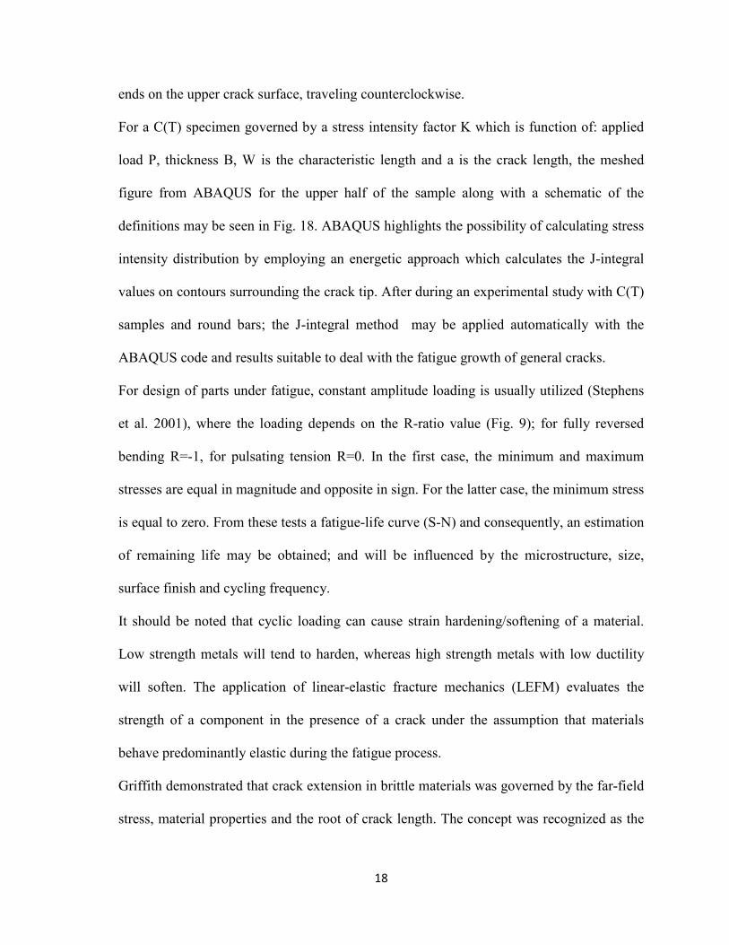
ends on the upper crack surface, traveling counterclockwise.

For a C(T) specimen governed by a stress intensity factor K which is function of: applied

load P, thickness B, W is the characteristic length and a is the crack length, the meshed

figure from ABAQUS for the upper half of the sample along with a schematic of the

definitions may be seen in Fig. 18. ABAQUS highlights the possibility of calculating stress

intensity distribution by employing an energetic approach which calculates the J-integral

values on contours surrounding the crack tip. After during an experimental study with C(T)

samples and round bars; the J-integral method may be applied automatically with the

ABAQUS code and results suitable to deal with the fatigue growth of general cracks.

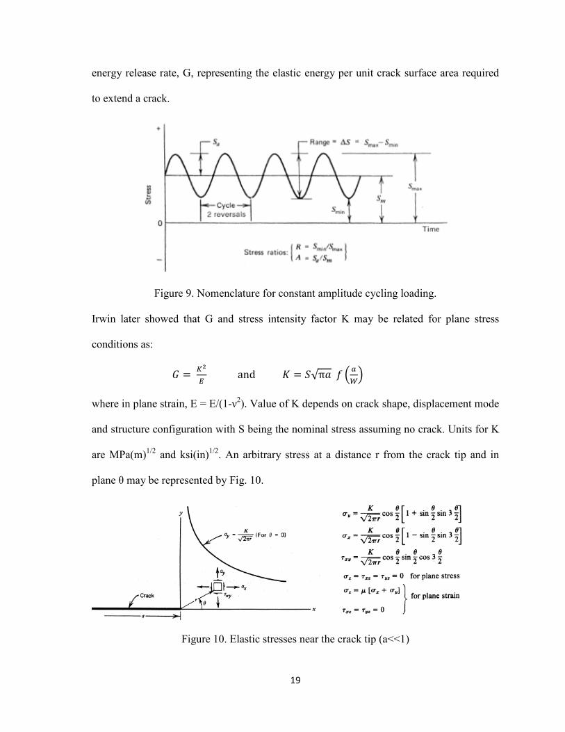
For design of parts under fatigue, constant amplitude loading is usually utilized (Stephens

et al. 2001), where the loading depends on the R-ratio value (Fig. 9); for fully reversed

bending R=-1, for pulsating tension R=0. In the first case, the minimum and maximum

stresses are equal in magnitude and opposite in sign. For the latter case, the minimum stress

is equal to zero. From these tests a fatigue-life curve (S-N) and consequently, an estimation

of remaining life may be obtained; and will be influenced by the microstructure, size,

surface finish and cycling frequency.

It should be noted that cyclic loading can cause strain hardening/softening of a material.

Low strength metals will tend to harden, whereas high strength metals with low ductility

will soften. The application of linear-elastic fracture mechanics (LEFM) evaluates the

strength of a component in the presence of a crack under the assumption that materials

behave predominantly elastic during the fatigue process.

Griffith demonstrated that crack extension in brittle materials was governed by the far-field

stress, material properties and the root of crack length. The concept was recognized as the

19

energy release rate, G, representing the elastic energy per unit crack surface area required

to extend a crack.

Figure 9. Nomenclature for constant amplitude cycling loading.

Irwin later showed that G and stress intensity factor K may be related for plane stress

conditions as:

' � �(�� ������������)*+������������ � ,-./��� 0�12�

where in plane strain, E = E/(1-ν2). Value of K depends on crack shape, displacement mode

and structure configuration with S being the nominal stress assuming no crack. Units for K

are MPa(m)1/2 and ksi(in)1/2. An arbitrary stress at a distance r from the crack tip and in

plane θ may be represented by Fig. 10.

Figure 10. Elastic stresses near the crack tip (a<<1)

20

It must be specified that the use of LEFM is restricted to small plastic zones at crack tip.

Stress intensity factors for different loading types inside the same mode may be added

together by using superposition, whereas K values for different modes (mode I, II, III)

cannot be added.

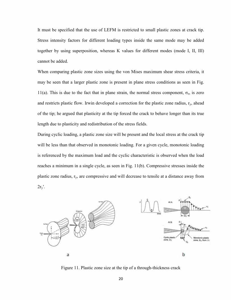
When comparing plastic zone sizes using the von Mises maximum shear stress criteria, it

may be seen that a larger plastic zone is present in plane stress conditions as seen in Fig.

11(a). This is due to the fact that in plane strain, the normal stress component, σz, is zero

and restricts plastic flow. Irwin developed a correction for the plastic zone radius, ry, ahead

of the tip; he argued that plasticity at the tip forced the crack to behave longer than its true

length due to plasticity and redistribution of the stress fields.

During cyclic loading, a plastic zone size will be present and the local stress at the crack tip

will be less than that observed in monotonic loading. For a given cycle, monotonic loading

is referenced by the maximum load and the cyclic characteristic is observed when the load

reaches a minimum in a single cycle, as seen in Fig. 11(b). Compressive stresses inside the

plastic zone radius, ry, are compressive and will decrease to tensile at a distance away from

2ry′.

Figure 11. Plastic zone size at the tip of a through-thickness crack

21

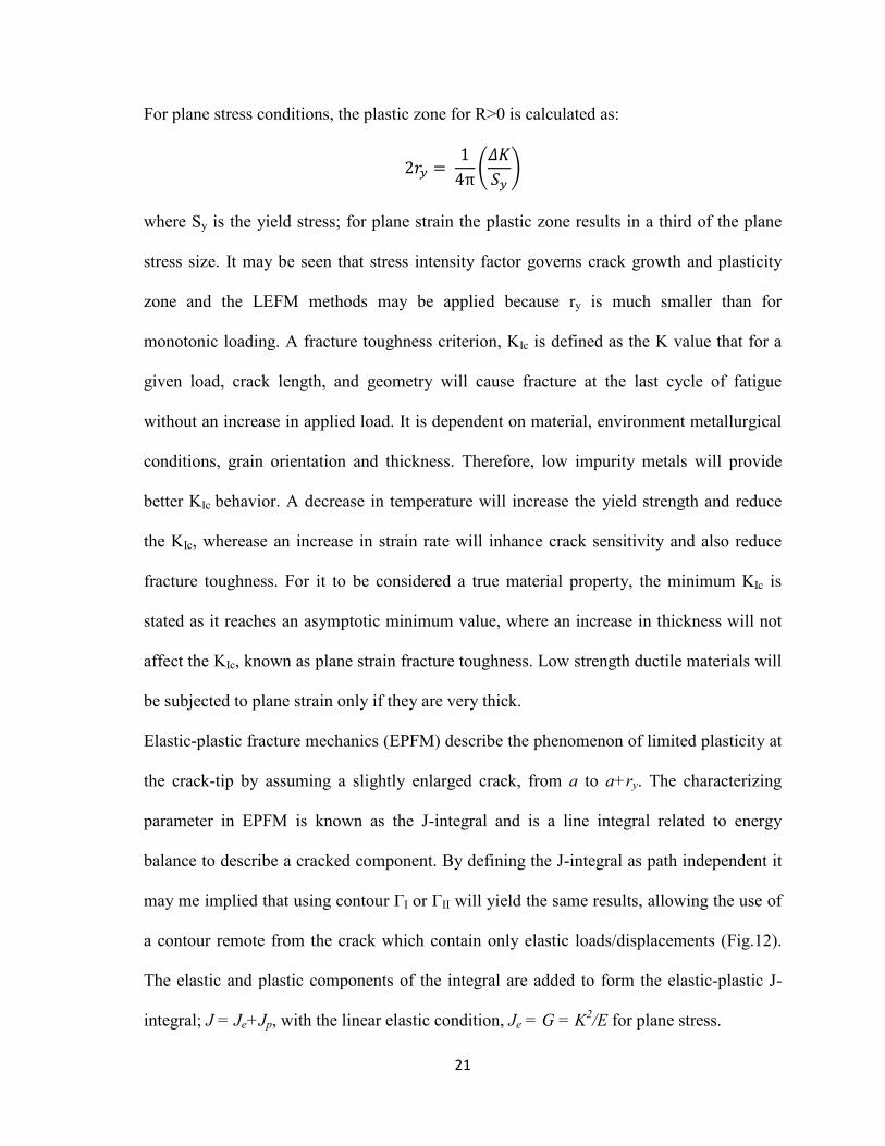
For plane stress conditions, the plastic zone for R>0 is calculated as:

345 �� 67.8��,5 9

where Sy is the yield stress; for plane strain the plastic zone results in a third of the plane

stress size. It may be seen that stress intensity factor governs crack growth and plasticity

zone and the LEFM methods may be applied because ry is much smaller than for

monotonic loading. A fracture toughness criterion, KIc is defined as the K value that for a

given load, crack length, and geometry will cause fracture at the last cycle of fatigue

without an increase in applied load. It is dependent on material, environment metallurgical

conditions, grain orientation and thickness. Therefore, low impurity metals will provide

better KIc behavior. A decrease in temperature will increase the yield strength and reduce

the KIc, wherease an increase in strain rate will inhance crack sensitivity and also reduce

fracture toughness. For it to be considered a true material property, the minimum KIc is

stated as it reaches an asymptotic minimum value, where an increase in thickness will not

affect the KIc, known as plane strain fracture toughness. Low strength ductile materials will

be subjected to plane strain only if they are very thick.

Elastic-plastic fracture mechanics (EPFM) describe the phenomenon of limited plasticity at

the crack-tip by assuming a slightly enlarged crack, from a to a+ry. The characterizing

parameter in EPFM is known as the J-integral and is a line integral related to energy

balance to describe a cracked component. By defining the J-integral as path independent it

may me implied that using contour ΓI or ΓII will yield the same results, allowing the use of

a contour remote from the crack which contain only elastic loads/displacements (Fig.12).

The elastic and plastic components of the integral are added to form the elastic-plastic J-

integral; J = Je+Jp, with the linear elastic condition, Je = G = K2/E for plane stress.

22

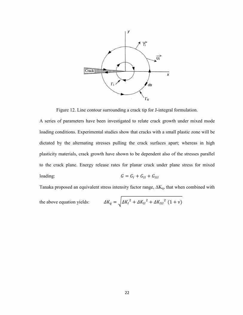
Figure 12. Line contour surrounding a crack tip for J-integral formulation.

A series of parameters have been investigated to relate crack growth under mixed mode

loading conditions. Experimental studies show that cracks with a small plastic zone will be

dictated by the alternating stresses pulling the crack surfaces apart; whereas in high

plasticity materials, crack growth have shown to be dependent also of the stresses parallel

to the crack plane. Energy release rates for planar crack under plane stress for mixed

loading: ' � '� : '�� : '��� Tanaka proposed an equivalent stress intensity factor range, ∆Kq, that when combined with

the above equation yields: ��; � ����� : ����� : ���������6 : <�

23

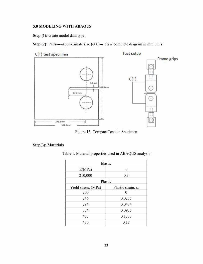
5.0 MODELING WITH ABAQUS

Step (1): create model data type

Step (2): Parts----Approximate size (600)--- draw complete diagram in mm units

Figure 13. Compact Tension Specimen

Step(3): Materials

Table 1. Material properties used in ABAQUS analysis

Elastic

E(MPa) ν

210,000 0.3

Plastic

Yield stress, (MPa) Plastic strain, εp 200 0

246 0.0235

294 0.0474

374 0.0935

437 0.1377

480 0.18

24

STEP (4): SECTION

Create section----shell---homogenious—continue—shell thickness 18.25 mm

STEP (5): SECTION ASSIGNMENT

Select whole section and click ok.

STEP (6): CREATE PARTITION

Partition face: Sketch---Select face +Auto calculate (done) ---select a plane—select point---

double click on a point

Step (7): Assembly

Instances-- dependent

Step (8): Steps

Steps---Double click

Step (9): Field output request

Right click—select manager—Edit

Step (10): History output request

Right click—select manager—Edit

Step (11): BC

Fixed: upper hole: U1=0, U2= 0 and UR3=0

Step (12): Load

Pressure load

25

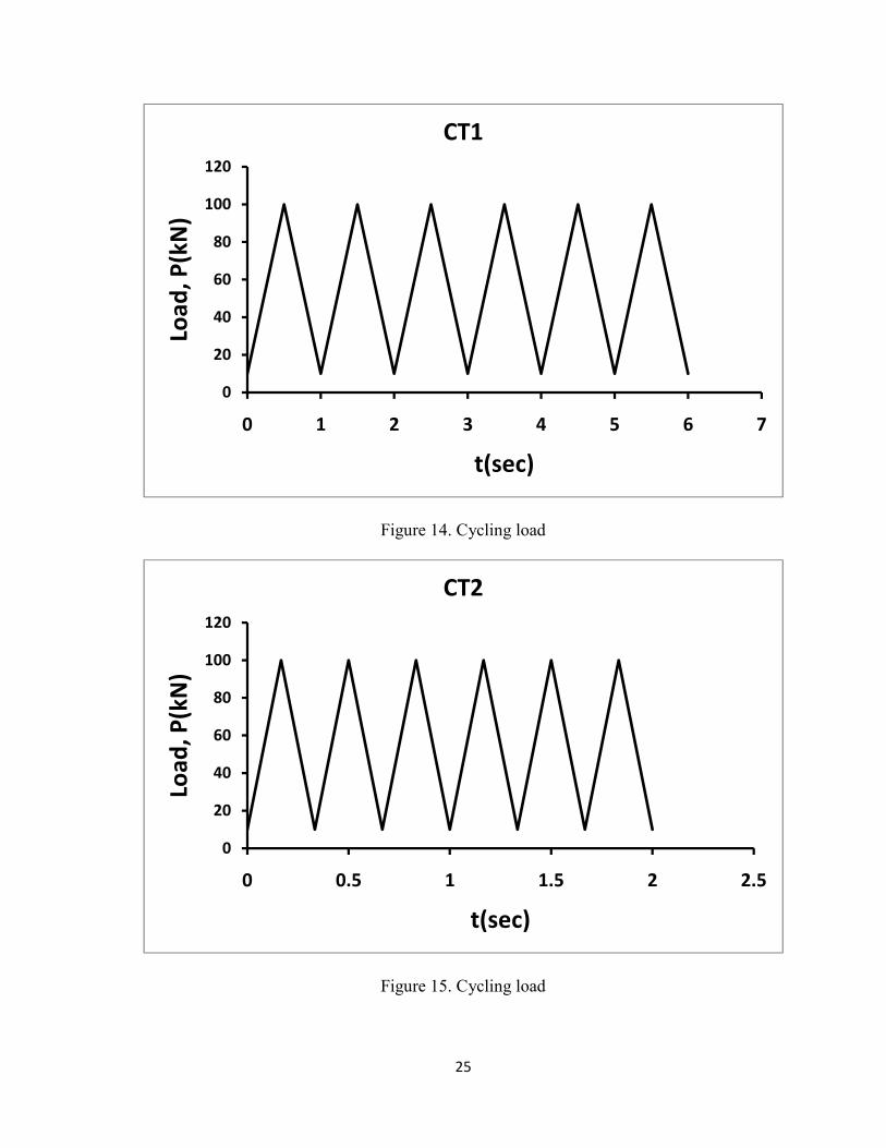
Figure 14. Cycling load

Figure 15. Cycling load

0

20

40

60

80

100

120

0 1 2 3 4 5 6 7

Load

, P(k

N)

t(sec)

CT1

0

20

40

60

80

100

120

0 0.5 1 1.5 2 2.5

Load

, P(k

N)

t(sec)

CT2

26

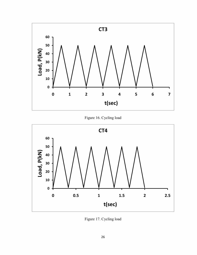
Figure 16. Cycling load

Figure 17. Cycling load

0

10

20

30

40

50

60

0 1 2 3 4 5 6 7

Load

, P(k

N)

t(sec)

CT3

0

10

20

30

40

50

60

0 0.5 1 1.5 2 2.5

Load

, P(k

N)

t(sec)

CT4

27

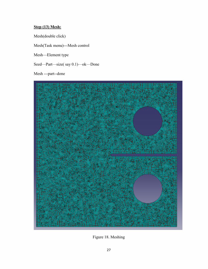
Step (13) Mesh:

Mesh(double click)

Mesh(Task menu)---Mesh control

Mesh—Element type

Seed—Part—size( say 0.1)—ok—Done

Mesh ---part--done

Figure 18. Meshing

28

Step(14): Jobs

---Create job

---Submit jobs

---Monitor

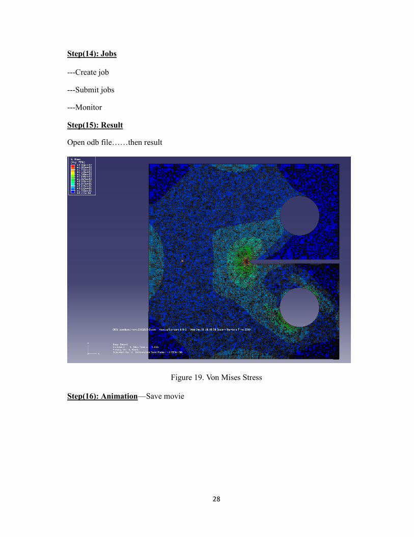
Step(15): Result

Open odb file……then result

Figure 19. Von Mises Stress

Step(16): Animation—Save movie

29

6.0 FUTURE STUDY

The performance and behavior characteristics of nearly all in-service structures can be

affected by damage resulting from external conditions such as weather, impact, loading

abrasion, operator abuse, or neglect (Bear et al., 2005). These factors can have serious

consequences on the in-service structures as related to safety, cost, and operational

capability. Therefore, the timely and accurate detection, characterization and monitoring of

structural cracking, corrosion, delamination, material degradation and other types of

damage are a major concern in the operational environment.

In recent years, Structural Health Monitoring is increasingly being evaluated by the

industry as a possible method to improve the safety and reliability of structures and thereby

reduce their operational cost. Structural health monitoring technology is perceived as a

revolutionary method of determining the integrity of structures involving the use of

multidisciplinary fields including sensors, materials, signal processing, system integration

and signal interpretation. The core of the technology is the development of self-sufficient

systems for the continuous monitoring, inspection and damage detection of structures with

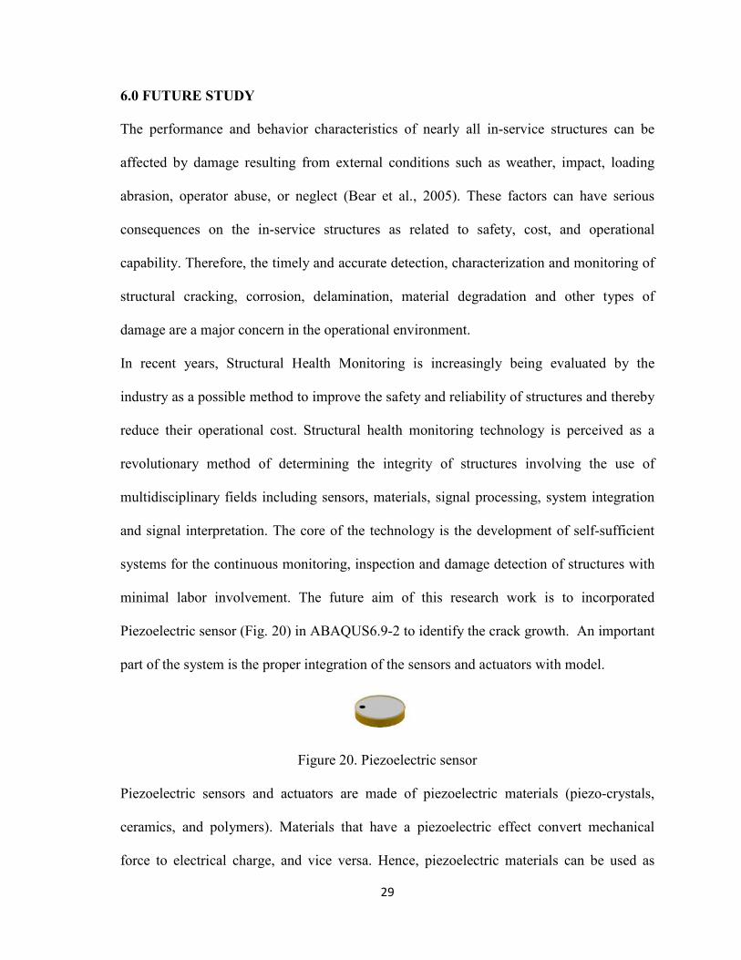
minimal labor involvement. The future aim of this research work is to incorporated

Piezoelectric sensor (Fig. 20) in ABAQUS6.9-2 to identify the crack growth. An important

part of the system is the proper integration of the sensors and actuators with model.

Figure 20. Piezoelectric sensor

Piezoelectric sensors and actuators are made of piezoelectric materials (piezo-crystals,

ceramics, and polymers). Materials that have a piezoelectric effect convert mechanical

force to electrical charge, and vice versa. Hence, piezoelectric materials can be used as

30

both sensors and actuators. As sensors, they produce an electrical signal when they are

physically deformed (strained). As actuators, they physically deform (expand, contract, or

shear) when an electrical charge is applied. Using this property, piezoelectric materials can

be used to measure stress and strain and can also be used to mechanically excite the

structure to propagate stress waves and induce internal vibrations. Inputting a time-varying

electrical signal to any of the actuators/sensors causes a propagating stress wave or

propagating mechanical deformation to emanate from the sensor/actuator and travel

through the material for detection by a plurality of neighboring sensors/actuators.

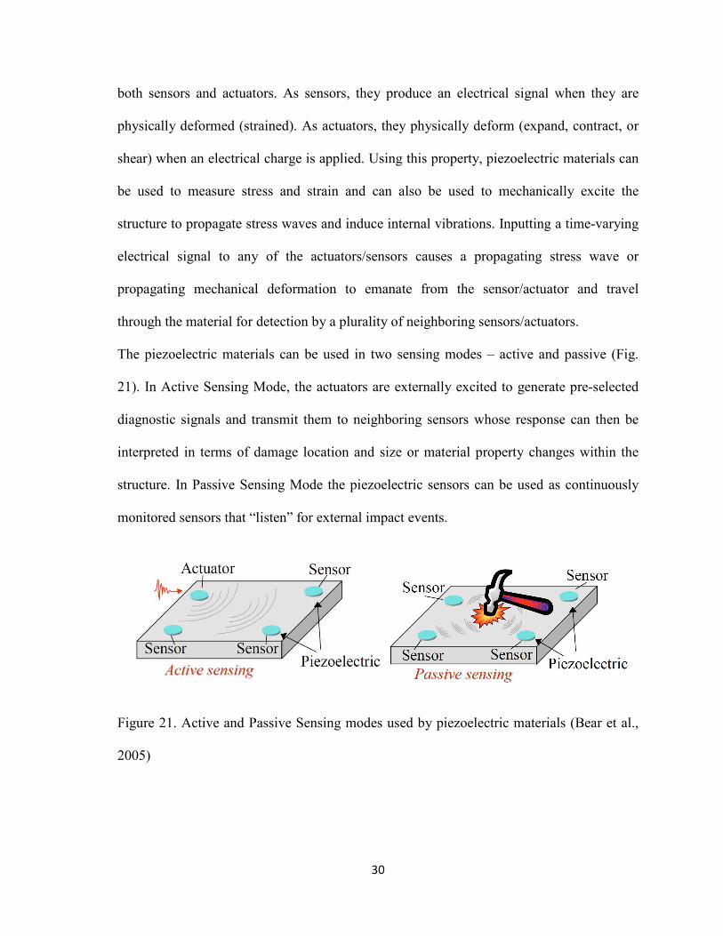
The piezoelectric materials can be used in two sensing modes – active and passive (Fig.

21). In Active Sensing Mode, the actuators are externally excited to generate pre-selected

diagnostic signals and transmit them to neighboring sensors whose response can then be

interpreted in terms of damage location and size or material property changes within the

structure. In Passive Sensing Mode the piezoelectric sensors can be used as continuously

monitored sensors that “listen” for external impact events.

Figure 21. Active and Passive Sensing modes used by piezoelectric materials (Bear et al.,

2005)

31

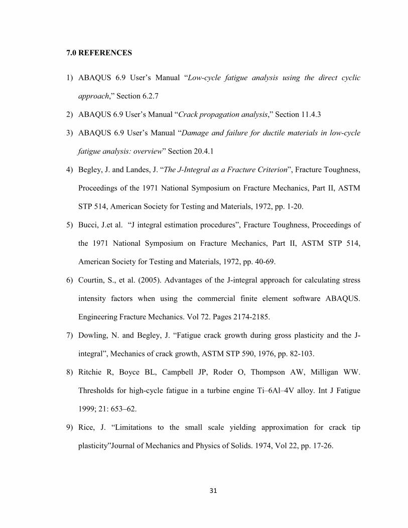
7.0 REFERENCES

1) ABAQUS 6.9 User’s Manual “Low-cycle fatigue analysis using the direct cyclic

approach,” Section 6.2.7

2) ABAQUS 6.9 User’s Manual “Crack propagation analysis,” Section 11.4.3

3) ABAQUS 6.9 User’s Manual “Damage and failure for ductile materials in low-cycle

fatigue analysis: overview” Section 20.4.1

4) Begley, J. and Landes, J. “The J-Integral as a Fracture Criterion”, Fracture Toughness,

Proceedings of the 1971 National Symposium on Fracture Mechanics, Part II, ASTM

STP 514, American Society for Testing and Materials, 1972, pp. 1-20.

5) Bucci, J.et al. “J integral estimation procedures”, Fracture Toughness, Proceedings of

the 1971 National Symposium on Fracture Mechanics, Part II, ASTM STP 514,

American Society for Testing and Materials, 1972, pp. 40-69.

6) Courtin, S., et al. (2005). Advantages of the J-integral approach for calculating stress

intensity factors when using the commercial finite element software ABAQUS.

Engineering Fracture Mechanics. Vol 72. Pages 2174-2185.

7) Dowling, N. and Begley, J. “Fatigue crack growth during gross plasticity and the J-

integral”, Mechanics of crack growth, ASTM STP 590, 1976, pp. 82-103.

8) Ritchie R, Boyce BL, Campbell JP, Roder O, Thompson AW, Milligan WW.

Thresholds for high-cycle fatigue in a turbine engine Ti–6Al–4V alloy. Int J Fatigue

1999; 21: 653–62.

9) Rice, J. “Limitations to the small scale yielding approximation for crack tip

plasticity”Journal of Mechanics and Physics of Solids. 1974, Vol 22, pp. 17-26.

32

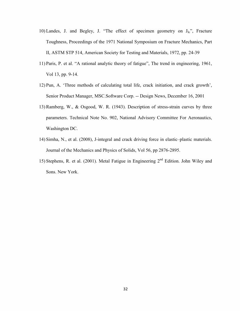
10) Landes, J. and Begley, J. “The effect of specimen geometry on JIc”, Fracture

Toughness, Proceedings of the 1971 National Symposium on Fracture Mechanics, Part

II, ASTM STP 514, American Society for Testing and Materials, 1972, pp. 24-39

11) Paris, P. et al. “A rational analytic theory of fatigue”, The trend in engineering, 1961,

Vol 13, pp. 9-14.

12) Pun, A. ‘Three methods of calculating total life, crack initiation, and crack growth’,

Senior Product Manager, MSC.Software Corp. -- Design News, December 16, 2001

13) Ramberg, W., & Osgood, W. R. (1943). Description of stress-strain curves by three

parameters. Technical Note No. 902, National Advisory Committee For Aeronautics,

Washington DC.

14) Simha, N., et al. (2008), J-integral and crack driving force in elastic–plastic materials.

Journal of the Mechanics and Physics of Solids, Vol 56, pp 2876-2895.

15) Stephens, R. et al. (2001). Metal Fatigue in Engineering 2nd Edition. John Wiley and

Sons. New York.