Embed Size (px)
Citation preview

Development and application of a New Zealand car ownership and traffic forecasting model
December 2009
Tim Conder
Booz & Co (New Zealand) Ltd
NZ Transport Agency research report 394

ISBN 978-0-478-35283-2 (print)
ISBN 978-0-478-35282-5 (electronic)
ISSN 1173-3756 (print)
ISSN 1173-3764 (electronic)
NZ Transport Agency
Private Bag 6995, Wellington 6141, New Zealand
Telephone 64 4 894 5400; facsimile 64 4 894 6100
www.nzta.govt.nz
Conder, T (2009) Development and application of New Zealand car ownership and traffic. NZ Transport
Agency research report 394. 166pp.
This publication is copyright © NZ Transport Agency 2009. Material in it may be reproduced for personal
or in-house use without formal permission or charge, provided suitable acknowledgement is made to this
publication and the NZ Transport Agency as the source. Requests and enquiries about the reproduction of
material in this publication for any other purpose should be made to the Research Programme Manager,
Programmes, Funding and Assessment, National Office, NZ Transport Agency, Private Bag 6995,
Wellington 6141.
Keywords: Car, forecasting, ownership
An important note for the reader
The NZ Transport Agency is a Crown entity established under the Land Transport Management Act 2003.
The objective of the Agency is to undertake its functions in a way that contributes to an affordable,
integrated, safe, responsive and sustainable land transport system. Each year, the NZ Transport Agency
funds innovative and relevant research that contributes to this objective.
The views expressed in research reports are the outcomes of the independent research, and should not be
regarded as being the opinion or responsibility of the NZ Transport Agency. The material contained in the
reports should not be construed in any way as policy adopted by the NZ Transport Agency or indeed any
agency of the NZ Government. The reports may, however, be used by NZ Government agencies as a
reference in the development of policy.
While research reports are believed to be correct at the time of their preparation, the NZ Transport Agency
and agents involved in their preparation and publication do not accept any liability for use of the research.
People using the research, whether directly or indirectly, should apply and rely on their own skill and
judgment. They should not rely on the contents of the research reports in isolation from other sources of
advice and information. If necessary, they should seek appropriate legal or other expert advice.

Acknowledgements
The author would like to thank Fergus Tait from MWH New Zealand Ltd and John Davies from Auckland
Regional Council for peer reviewing this report.
The author would also like to thank staff from the NZ Transport Authority, Ministry of Transport, Statistics
New Zealand and local territorial authorities who provided data and information used for this research.
Abbreviations and acronyms
ADT Average daily traffic
ASC Alternative specific constant
BTRE Bureau of Transport and Regional Economics (Australia)
DETR Department for the Environment, Transport and the Regions (UK), now the DfT
DfT Department for Transport (UK), formerly the DETR
EEM Economic evaluation manual
GDP Gross domestic product
VKT Vehicle kilometres travelled
LMS The Netherlands government transport forecasting model system,
MoT Ministry of Transport
NRTF model National road traffic forecasts model (UK)
NZTA New Zealand Transport Authority (merger of Transit NZ and Land Transport NZ)
PEM Project evaluation manual (now EEM vol 1)
PT Public transport
RUC Road user charges
STM Strategic travel model (Sydney)
TDM Travel demand management
TLA Territorial local authority
Transit Transit New Zealand
TRC Transport Registry Centre
TTM Tauranga transport model
VFEM Vehicle fleet emissions model
VKT Vehicle kilometres travelled
WoF Warrant of fitness
WTSM Wellington transport strategy model

5
Contents
Executive summary ................................................................................................................................................... 9
Abstract ........................................................................................................................................................................10
1 Introduction...................................................................................................................................................11
1.1 Background and context ....................................................................................... 11
1.2 Project purpose ..................................................................................................... 11
1.3 Project scope......................................................................................................... 12
1.4 Project process...................................................................................................... 12
1.5 Structure of the report .......................................................................................... 12
2 Appraisal of New Zealand car ownership and use trends........................................................14
2.1 New Zealand vehicle ownership............................................................................. 14 2.1.1 Sources for vehicle registration data......................................................... 14 2.1.2 Best database ........................................................................................... 15 2.1.3 Project estimates of motor vehicle ownership in New Zealand .................. 16 2.1.4 Analysis of past trends ............................................................................. 19 2.1.5 Vehicle ownership in different areas: census data..................................... 21
2.2 New Zealand car use trends .................................................................................. 25 2.2.1 New Zealand Household Travel Survey...................................................... 25 2.2.2 Ministry of Transport – warrant of fitness data ......................................... 26 2.2.3 Traffic count data ..................................................................................... 27 2.2.4 Regional household interview surveys ...................................................... 28 2.2.5 Impacts of transport fuel price changes.................................................... 29
2.3 Comparison with international data....................................................................... 30
2.4 Conclusions .......................................................................................................... 32
3 Update of a New Zealand aggregate car ownership model .....................................................33
3.1 The Booz aggregate car ownership model ............................................................. 33 3.1.1 Introduction.............................................................................................. 33 3.1.2 Basis for forecasting vehicle ownership .................................................... 33 3.1.3 Saturation level......................................................................................... 33 3.1.4 Growth to saturation................................................................................. 37 3.1.5 New Zealand car ownership forecasts ....................................................... 40
3.2 Comparison with other New Zealand model forms ................................................ 41 3.2.1 Prediction comparison: 1997–2006 .......................................................... 43
3.3 Conclusions .......................................................................................................... 43
4 Development of policy and functional requirements .................................................................45
4.1 Car ownership and use ‘needs’ survey................................................................... 45 4.1.1 Respondents............................................................................................. 45

6
4.2 Survey results........................................................................................................ 46 4.2.1 Current sources of car ownership and use data ........................................ 46 4.2.2 Current uses of car ownership data .......................................................... 46 4.2.3 Future uses of car ownership data ............................................................ 47 4.2.4 Potential features of future car ownership model...................................... 47 4.2.5 Other comments....................................................................................... 52
4.3 Conclusions .......................................................................................................... 52
5 Review of New Zealand modelling practices ................................................................................. 54
5.1 National modelling methodologies........................................................................ 54 5.1.1 MoT vehicle fleet emissions model ........................................................... 54
5.2 Regional modelling methodologies ....................................................................... 57 5.2.1 Auckland regional transport model........................................................... 58 5.2.2 Wellington transport strategy model......................................................... 60 5.2.3 Christchurch transport model ................................................................... 64 5.2.4 Tauranga transportation model ................................................................ 66
5.3 New Zealand car ownership and use literature ...................................................... 68 5.3.1 Vehicle availability forecasting model, Travis Morgan (1992) .................... 68 5.3.2 Model for forecasting vehicle ownership In New Zealand,
Booz Allen Hamilton (2000) ...................................................................... 70 5.3.3 Traffic growth prediction, Koorey et al (2000) .......................................... 73 5.3.4 Economic evaluation manual, Land Transport NZ (2006) .......................... 76 5.3.5 National Land Transport Programme 2007/08 ......................................... 76 5.3.6 Impacts of transport fuel price changes, Booz Allen Hamilton (2006) ....... 77
5.4 Conclusions .......................................................................................................... 81
6 Review of international evidence and forecasting practices.................................................. 83
6.1 Overview of car ownership modelling .................................................................... 83 6.1.1 Aggregate time series approaches ............................................................ 83 6.1.2 Static disaggregate approaches ................................................................ 84 6.1.3 The cohort approach ................................................................................ 84
6.2 Discussion of general model archetypes................................................................ 85 6.2.1 Aggregate time series model .................................................................... 87 6.2.2 Aggregate market model .......................................................................... 89 6.2.3 Aggregate cohort model ........................................................................... 90 6.2.4 Heuristic simulation model ....................................................................... 90 6.2.5 Static disaggregate model......................................................................... 90 6.2.6 Indirect utility model................................................................................. 91 6.2.7 Dynamic transaction model ...................................................................... 92
6.3 Features of key model types.................................................................................. 92 6.3.1 Aggregate time series model .................................................................... 93 6.3.2 Static disaggregate model......................................................................... 95 6.3.3 Aggregate market model .......................................................................... 98 6.3.4 Summary of key model types .................................................................... 99

7
6.4 Examples of international models ....................................................................... 100
7 Development of a recommended New Zealand modelling framework............................105
7.1 Introduction ........................................................................................................ 105
7.2 Potential model types.......................................................................................... 105 7.2.1 Aggregate time series models ................................................................ 105 7.2.2 Static disaggregate models..................................................................... 106 7.2.3 Aggregate car market models................................................................. 107 7.2.4 Recommendation.................................................................................... 108
7.3 Recommended long-term future modelling methodology ................................... 108 7.3.1 Overview and structure........................................................................... 109 7.3.2 Data requirements .................................................................................. 114 7.3.3 Model development and data collection process..................................... 116 7.3.4 Use of the model .................................................................................... 116
7.4 Short- to medium-term modelling methodology ................................................ 117 7.4.1 Short- to medium-term framework ........................................................ 117 7.4.2 National aggregate model: MoT VFEM..................................................... 118 7.4.3 Agreed set of inputs and assumptions.................................................... 118
7.5 Summary............................................................................................................. 119
8 Conclusions and recommendations.................................................................................................120
8.1 Conclusions ........................................................................................................ 120
8.2 Recommendations............................................................................................... 121
9 References...................................................................................................................................................123
Appendix A: New Zealand vehicle ownership data ..............................................................................126
Appendix B: Components of general model archetypes....................................................................130
Appendix C: Model archetypes influencing factors .............................................................................133
Appendix D: Summary of key model types..............................................................................................137
Appendix E: Review of international models ..........................................................................................142

8
9
Executive summary
This report investigates improved methods for forecasting car ownership and use in New Zealand. The
research was conducted by Booz & Company (New Zealand) Ltd in 2007/08.
Car ownership and use in New Zealand
Examination of New Zealand car ownership and use data shows the following:
Car ownership has continued to increase. In 1970 car ownership was 0.310 cars per person; by 2005
it had risen to 0.574 cars per person.
There appears to be a relationship between times of increasing GDP per person and decreasing car
prices corresponding to increased car ownership per person.
New Zealand continues to have one of the highest rates of car ownership in the world.
Information on vehicle kilometres travelled has been collected since 2001, using odometer readings
taken during vehicle warrant of fitness inspections. This data shows that light vehicle travel per
person increased between 2001 and 2005, but decreased in 2006. Average annual travel per vehicle
has been decreasing since 2002.
Previous research has shown that increased petrol prices result in less fuel consumption per person.
This could explain why since 2002 light vehicle travel per person has decreased.
Aggregate car ownership model
As part of the research an aggregate car ownership model for New Zealand was updated. The following
key conclusions have been reached from the development and application of this model, which can
forecast future car ownership:
The current level of car ownership in New Zealand, approximately 0.58 cars per capita, is below the
saturation level of car ownership which is estimated to be in the range of 0.67 cars per capita (lower)
to 0.75 cars per capita (upper). By 2041 the saturation level is predicted to increase, due to changes in
age distribution, to between 0.71 cars per capita (lower) and 0.79 cars per capita (upper).
Elasticities of GDP per capita and car price index can be used to predict future changes in car
ownership, particularly in the short to medium term. These appear to be a strong set of relationships
(ie economic conditions and car prices are predicted to have a significant impact on future car
ownership).
There is considerable uncertainty over factors that could have a significant impact on car ownership.
For example it is unlikely that the real downward trend in the car price index that has occurred over
the last 30 years will continue. The ability to forecast future car ownership is dependent on the ability
to accurately forecast changes in GDP and car prices.
Development of a car ownership and use framework
The development of a New Zealand car ownership and use modelling framework was based on a user
needs survey and a review of current New Zealand and international practices.
The user needs survey was conducted with transport practitioners in New Zealand. Results suggested that
a modelling methodology for car ownership and use should ideally:

Development and application of a New Zealand car ownership and traffic forecasting model
10
be segmented by private vehicles (private and company ownership)
be applied to national, regional and local contexts
focus on forecasting within a 25-year horizon
segment vehicles by fuel type/efficiency and split between private and business
be sensitive to changes in fixed/variable costs, in particular changes in fuel taxes and road user
charges, changes in income and the level of public transport supply
have outputs which include vehicle numbers, usage, emissions and fuel consumption measures and to
a lesser extent, government revenue.
The review of New Zealand modelling practices and literature identified a lack of a consistent approach to
forecasting car ownership in New Zealand. While some of the regional models are regulated by national
forecasts for car ownership, they are not the same forecasts. There does not appear to be a consistent set
of key input assumptions for these model forecasts (eg future GDP or income, car prices). As these
regional models are used to predict future transport requirements, the outputs forming an input to project
prioritisation, it would be highly desirable if the forecasting of car ownership was undertaken on a
consistent basis. As such, what appears to be lacking is an integrated framework for forecasting car
ownership.
Following a review of user needs against local and international practice, it was concluded that the
development of a national static disaggregate model was the recommended modelling methodology for car
ownership and use. This is because it provides the desired level of functionality, is able to test many policy
variables (eg public transport provision) and there is a large international body of experience to draw upon.
However it is recognised that developing a national static disaggregate car ownership model for
New Zealand is a substantial undertaking and the development costs are likely to be significant.
Consequently, there is merit in exploring a short- to medium-term modelling framework which would
build upon existing models to provide the basis for forecasting car ownership and use, and ensure
national consistency.
Abstract
This research investigated improved methods for forecasting car ownership and use in New Zealand. It
compiled and reviewed current data and information on car ownership and use. From this data an
aggregate car ownership model for New Zealand was developed. This model predicts that economic
conditions and car prices will have a significant impact on future car ownership. A future framework for
forecasting car ownership and use in New Zealand was developed, based on reviewing current
New Zealand practice, international practice and by undertaking a user needs survey. The resulting
recommended long-term framework is a national static disaggregate model. A short- to medium-term
framework was also developed which provides an intermediate step to address some of the current
shortcomings in New Zealand practices. The research was primarily undertaken in 2007/2008.

1 Introduction
11
1 Introduction
1.1 Background and context
New Zealand does not have a national traffic forecasting model (unlike many countries), nor does it have a
standardised methodology for traffic forecasting across the various major urban centres. Given that the
majority of contemplated investment in increasing road network capacity over the next 10–20 years is
planned to be in the major urban areas, this is a deficiency in terms of project planning and evaluation.
The NZTA Economic evaluation manual (EEM) provides some guidelines on traffic growth forecasts, but
these are largely based on the extension of historical trends, with little regard to issues such as
population and age structure changes, increasing fuel prices and the potential approach of saturation
levels of vehicle ownership and use. As stated in the EEM:
Historical traffic growth rates (in arithmetical terms) are generally considered to provide a
sound basis for predicting future traffic demand provided there are no traffic restraints.
This is a simplistic approach compared with those adopted in most other developed countries: ‘best
practice’ approaches adopted elsewhere could be expected to provide not only better ‘central estimates’
but also much improved information on the sensitivity of estimates to a range of significant variables.
The aim of the project was improve understanding on forecasting future car ownership and use (traffic
growth) in New Zealand, and to provide a projection of likely future car ownership and the development of
an appropriate model methodology. This methodology would provide a key input to the development of a
New Zealand national traffic model (which, we understand, is currently under discussion), and also to the
potential upgrading of the Ministry of Transport (MoT) vehicle fleet emissions model (VFEM).
1.2 Project purpose
In order to achieve its objective of developing and showing the application of improved methods for
forecasting future car ownership and use in New Zealand, the project.
focused on methods for forecasting car ownership and use at both national and regional/sub-regional
levels, over a timescale of at least 20 years. Traffic trends by other vehicle types (including trucks)
were not addressed by this research
appraised and built on best practices in car ownership and use modelling adopted internationally
had regard to and (as appropriate) built on practices adopted in New Zealand, particularly those
incorporated in the regional transport models in the main centres
had a primary emphasis on methodology and model structure, rather than on providing specific
forecasts.
While the project provided some (illustrative) scenarios for future car ownership trends based on
assumptions about input variables, it is likely that subsequent work will be necessary to further investigate
likely trends in input variables (eg fuel prices) in order to generate a firm set of traffic trend scenarios for
use in future traffic forecasting work.

Development and application of a New Zealand car ownership and traffic forecasting model
12
1.3 Project scope
The scope of this research project was to develop two main outputs:
1 To update an aggregate car ownership forecasting model using historical data, and including some of
the more traditional response variables such as car prices per GDP with saturation included. This
model would provide forecasts of car ownership at an aggregate level and build upon work already
undertaken in previous research (Booz Allen Hamilton 2000).
2 To develop a modelling framework (but no working model) for future development. This framework
would be constructed by comparing policy and functionality requirements (through the use of a needs
survey) with current modelling methodologies (international and New Zealand) and data availability. A
recommendation would be made as to whether the modelling framework would be best delivered as
an enhancement to an existing methodology, or as a new methodology.
As part of these two main outputs, the scope also included:
appraisal of New Zealand car ownership data and use trends
review of New Zealand modelling practices and literature
review of international evidence and forecasting practices
development of policy and functional requirements
1.4 Project process
The project was undertaken by developing seven separate working papers each of which focused on a
particular aspect of the research. The working papers were peer reviewed and then combined into this
overall report. Research was primarily undertaken in 2007/2008
1.5 Structure of the report
The structure of the remainder of this report is as follows:
Part A: New Zealand trends and an update of an aggregate model for NZ
Section 2: Appraisal of New Zealand car ownership and use trends
Section 3: Aggregate model for car ownership
Part B: Development of a New Zealand modelling framework
Section 4: Development of policy and functional requirements (user survey)
Section 5: Review of New Zealand modelling practices
Section 6: Review of international evidence and forecasting practices
Section 7: Development of a recommended New Zealand modelling framework
Section 8: Conclusions and recommendations

1 Introduction
13
Figure 1.1 shows the general relationship between the two main parts of this report. The numerical circles
in this figure represent the report section numbers. As shown in this figure, the two main outputs from
this research are updating an aggregate model for car ownership (Part A) and the development of a
recommended New Zealand modelling framework (Part B).
Figure 1.1 Relationship between report sections
Appraisal of NZ car ownership &
use trends
Part B
Review of NZ modelling practices
Review of international evidence & practices
Update NZ Aggregate Model
Part A
Development of functional
requirements
Development of a NZ modelling
framework
➁
➂
➃ ➅
➆
➄

Development and application of a New Zealand car ownership and traffic forecasting model
14
2 Appraisal of New Zealand car ownership and use trends
2.1 New Zealand vehicle ownership
2.1.1 Sources for vehicle registration data
The various data sources for vehicle registrations in New Zealand have previously been investigated in
considerable detail by Booz Allen Hamilton (2000) and Beca Carter Hollings & Ferner (Beca) (2003). The
key conclusions from this work are detailed below:
It was originally expected that a time series of historical motor vehicle ownership in New Zealand could be
taken directly from published statistics. However, this proved not to be the case, particularly because of
changes in the last few decades in the ‘standard’ method of recording the number of motor vehicles
registered. Hence considerable investigations were made to estimate a consistent and realistic time series
of motor vehicle ownership at the national level. These investigations are summarised below and a ‘best’
time series has been derived.
New Zealand vehicle registrations are maintained by NZTA’s Transport Registry Centre (TRC). Three time
series, which have been derived from TRC data, are readily available:
Tables of ‘licensed motor vehicles’ in the transport section of the New Zealand Official Yearbook. This
series is based on the TRC March quarterly return. It presents the number of motor vehicles licensed
at 31 March and 30 June each year. Figures are available from 1951, broken down by vehicle type.
Tables of vehicles registered, in Motor vehicle crashes in New Zealand, a report produced annually by
the MoT (previously titled Motor accidents in New Zealand). This series was originally based on the
TRC December quarterly return, and represented the numbers of vehicles registered at 31 December
each year. It records some vehicle categories not included in the yearbook series: exempt vehicles,
tractors, trade plates and caravans. Only an aggregate figure is provided.
Tables of vehicles licensed by quarter prior to 1987, and by month after 1987, held by Statistics NZ.
This series is also based on the TRC returns, is available from 1970, and is broken down by vehicle
type.
A new licensing system was introduced in 1987. No figures were provided by TRC in 1987, and the 1988
figures were some 10% lower than those for 1986. Given the long-running upward trend in motor vehicle
registrations this was considered unrealistic, and prompted further investigations about the compilation of
the figures. Previous discussions with the TRC and staff of the Land Transport Safety Authority (LTSA) (now
NZTA) provided the following information.
Prior to 1986:
motor registration had a manual recording system
all motor vehicles were relicensed annually at the same time of the year

2 Appraisal of New Zealand car ownership and use trends
15
deregistered vehicles were only deleted from the record of licensed vehicles once a year, following the
end of the June quarter. All of the quarterly returns therefore included vehicles scrapped
(deregistered)
the quarterly returns represented the total number of licensed vehicles at the end of that particular
quarter – that is, all vehicles licensed at the end of the quarter plus any other vehicles which were
licensed from 1 July for which licences may have subsequently been deregistered.
From 1987, when a computerised recording system was installed, until the present:
statistics represent the number of current licensed vehicles at the date of reporting
deregistered vehicles are removed from the computer records immediately and therefore from the
number of licensed vehicles at the date of reporting
as the result of a new spread relicensing system also introduced in 1987, licensing periods of both six
months and 12 months, and licence expiry dates are spread throughout the year
the change to reporting statistics ‘as at’ a certain date rather than ‘for the year ended’, and the new
spread relicensing system means that a significant proportion of vehicles are not recorded in the
annual statistics because their licence was paid after the due date.
It was concluded from this that:
TRC statistics prior to 1987 were an over-estimate of the number of vehicles licensed at any one time,
due to deregistered vehicles not being removed from the totals
TRC statistics after 1987 represent the number of vehicles for which licences were strictly valid at any
one time, not allowing for any late relicensing. These should be added in to reflect the total ‘active’
vehicles at any one time
census data is also readily available and is discussed in further detail in later sections of this report.
However the census is only undertaken every five years and primarily records motor vehicles available
to households on census night.
2.1.2 Best database
Having reviewed the three main sources of time series data for New Zealand motor vehicle ownership, it
was decided to use the Statistics NZ data (September quarter) as the basis from which to derive a
consistent time series.
This decision was based on the following considerations.
All three time series are based on the TRC data, and would be suitable as the basis for a historical
time series.
The New Zealand Official Yearbook data, which reports licensed vehicles at the end of March each
year, includes a higher proportion of scrapped vehicles for the period prior to 1987 than does the
Statistics NZ data. It would therefore be a less accurate representation of active vehicles than the
Statistics NZ data.

Development and application of a New Zealand car ownership and traffic forecasting model
16
The MoT (previously LTSA) figures would also be a less accurate representation of active vehicles than
the Statistics NZ data. They represent licensed vehicles at the end of December each year and, since
1986, have been estimated using a simple spreadsheet model.
The three time series are shown in table A.1 in appendix A and in figure 2.1 below.
Figure 2.1 Licensed motor vehicles time series
2.1.3 Project estimates of motor vehicle ownership in New Zealand
For purposes of previous research and this project, a consistent time series of annual figures for the
number of ‘active’ motor vehicles (cars, motorcycles) in New Zealand was required.
As detailed in section 2.1.2 above, it was decided to use the September quarter data from the Statistics NZ
database as the basis for this time series. However, as discussed below, several issues had to be
addressed in developing the time series.
Scrapped vehicles
Prior to the introduction of the computer-based relicensing system in 1986 vehicles which were scrapped
during the year continued to be counted as being licensed until the end of June, at which time all
deregistered vehicles were removed from the records. Thus, the TRC-based records always included some
‘inactive’ vehicles, with the number of these increasing during the year from July to June.
Analysis conducted by the Land Transport Division of the MoT in the early 1990s concluded that the
proportion of scrapped vehicles ranged from between 3% pa and 6% pa of licensed vehicles for the period
1970 to 1992, averaging out to 4.4% pa. Using the September quarter figures minimised the number of
scrapped vehicles being counted as ‘active’; however, there would still be a small number of scrapped
vehicles included in Statistics NZ’s numbers. The pre-1986 figures have therefore been adjusted
downwards by 1% to reflect this (1% being one quarter of the average annual proportion).
0.0
500.0
1,000.0
1,500.0
2,000.0
2,500.0
3,000.0
3,500.0
1951
1953
1955
1957
1959
1961
1963
1965
1967
1969
1971
1973
1975
1977
1979
1981
1983
1985
1987
1989
1991
1993
1995
1997
1999
2001
2003
2005
Year
NU
mb
er o
f M
oto
r V
ehic
les
(000
s)
Yearbook
MoT
Statistics NZ

2 Appraisal of New Zealand car ownership and use trends
17
Late relicensing
Prior to 1986 all vehicles were counted by the TRC as being licensed, unless they had actually been
deregistered. This meant that vehicles which were relicensed late were also counted in the total of licensed
vehicles. However, since 1986 the figures released by the TRC to Statistics NZ have been the actual
number of vehicles with current licences. This means that the post-1986 figures are an under-estimate of
‘active’ vehicles as they do not include late registrations.
An analysis by the MoT Land Transport Division in 1992 over a six-month period concluded that about 8% of
active vehicles were not relicensed at any one time. Booz Allen Hamilton (2000) analysed two sets of motor
vehicle licensing data, one of which was gathered by the MoT and one by the LTSA. This analysis found that
the number of all ‘active’ vehicles unlicensed at any one time was 4% and 5.5% of the total licensed vehicles
(this analysis assumed that all vehicles relicensed within 12 months of their anniversary date were ‘active’).
We have therefore increased the Statistics NZ post-1986 data by 5% to account for late registrations.
Semi-permanently unlicensed
We have not made any adjustments for vehicles which are unlicensed for more than 12 months, although
it could be argued these should be made. The MoT's broad estimates for these are about 1–2% of all
vehicles (reliable data is not available).
Vehicle categories
Vehicle categories have changed over time. However, the Statistics NZ data is sufficiently detailed so that
this variation could be accounted for in the vehicle totals.
2.1.3.1 Results
After applying the above adjustments to each vehicle type, table A.2 in appendix A shows our estimates of
annual motor vehicle ownership in New Zealand, while table A.3 shows the estimate by vehicle type.
The adjustments involved:
a reduction in the Statistics NZ September figures pre-1986 of 1%
an increase in the Statistics NZ September figures post-1987 of 5%.
2.1.3.2 Trends in vehicle ownership
Figure 2.2 shows the trends in motor vehicle ownership in NZ during the period 1970–2006, using our
best estimate, plus the breakdown into main vehicle categories, ie cars, motorcycles, goods and buses.

Development and application of a New Zealand car ownership and traffic forecasting model
18
Figure 2.2 NZ motor vehicle ownership 1970–2006
Key features of the results include (based on the best estimate vehicle ownership):
There was a total of 2.767 million motor vehicles at September 2006.
This total comprised 82.4% cars, 2.2% motorcycles, 14.8% goods and 0.6% buses.
Numbers of cars and good vehicles increased almost every year throughout this period. Apart from
the 1986/87 ‘blip’, which has been resolved partially by the adjustments made, the only recent
exception to this steady upward trend was in 1992 when the number of cars dropped slightly for the
first time in 20 years.
Numbers of motorcycles increased rapidly in the 1970s, peaked in the mid-1980s and have since
decreased by almost half.
Figure 2.3 shows the trend in cars and motorcycles per person over the last 35 years. Table 2.1
summarises the increases in car ownership over the consecutive five-year periods during that time.
Figure 2.3 Motor vehicle ownership per person 1970–2006
0.000
0.100
0.200
0.300
0.400
0.500
0.600
0.700
1970 1972 1974 1976 1978 1980 1982 1984 1986 1988 1990 1992 1994 1996 1998 2000 2002 2004 2006
Y
NU
mb
er o
f M
oto
r V
ehic
les
per
Per
son
Cars
Motorcycles
0.0
500.0
1000.0
1500.0
2000.0
2500.0
3000.0
1970 1972 1974 1976 1978 1980 1982 1984 1986 1988 1990 1992 1994 1996 1998 2000 2002 2004 2006
Year
Nu
mb
er o
f M
oto
r V
ehic
les
(000
s)
Cars
Mcycs
Goods
Buses

2 Appraisal of New Zealand car ownership and use trends
19
Table 2.1 Increase in car ownership 1970–2005
5-year increase in cars/person 5 yrs ending End cars per person
Absolute Total % Ave % pa
1970 0.310 - - -
1975 0.367 0.057 18.3% 3.4%
1980 0.402 0.034 9.4% 1.8%
1985 0.442 0.040 10.0% 1.9%
1990 0.476 0.034 7.6% 1.5%
1995 0.493 0.018 3.7% 0.7%
2000 0.523 0.030 6.0% 1.2%
2005 0.574 0.051 9.8% 1.9%
It is apparent that:
The absolute change in cars per person over each five-year period decreased between 1970 and
1995. However, since 1995 the absolute change has been increasing in each five-year period. The
absolute change in cars per person was at its highest level in the five-year period to 1975, with an
average of 57 cars per 1000 persons, and dropping to 18 cars per 1000 persons for the period to
1995. However, for the five-year period to 2005 the absolute change increased to 51 cars per 1000
persons.
Similar to the absolute change, the average percentage change per annum fell between 1970 and
1995. However, the average percentage change has increased since 1995.
The previous analysis of the trends used the data up until 1995 (Booz Allen Hamilton 2000). The data
to 1995 showed that car ownership was increasing at a reduced rate over time, indicating that car
ownership could be approaching saturation level. However, since 1995 the rate of change of car
ownership has again been increasing. Following little change in car ownership per person during the
mid-1990s, car ownership per person increased significantly during the late 1990s and early 2000s.
2.1.4 Analysis of past trends
2.1.4.1 Data sources
For analysis purposes, time series data has been assembled based on the following:
1 New Zealand population total (Statistics NZ data sources)
a mean population for year ending 31 March for years 1955–1996 (the mean population concept
was discontinued in 1997 and replaced with a resident population estimate)
b resident population for year ending 31 March for years 1992–2006 (while the population numbers
have been developed on different basis, analysis of the overlapping years when both data was
available shows a difference of only 2% to 2.7%)
2 New Zealand real GDP (Statistics NZ data sources)
a annual GDP for year ending 31 March

Development and application of a New Zealand car ownership and traffic forecasting model
20
b for years 1955–1996, expressed in constant prices ($1982/83)
c for years 1988–2007, expressed in constant prices ($1995/96)
d all GDP data converted to $1982/83
3 New Zealand average car purchase prices (Statistics NZ special analysis)
a average prices of all cars purchased (new and second-hand) in New Zealand for year ending 31
March from 1970–2006, as used in CPI composition
2.1.4.2 Analysis of trends
An analysis was undertaken to investigate the extent to which car ownership levels might be affected by
changes in real income (GDP per person) and changes in real car prices.
Figure 2.4 shows the increasing trend in GDP per person while figure 2.5 shows the generally decreasing
trend in average real car prices. As shown in figure 2.3 there was an increase in car ownership per person
during this period.
Figure 2.4 Trends in NZ GDP per person 1970–2006
Figure 2.5 Trends in average real car prices: 1970–2006
0
2,000
4,000
6,000
8,000
10,000
12,000
14,000
16,000
1970
1972
1974
1976
1978
1980
1982
1984
1986
1988
1990
1992
1994
1996
1998
2000
2002
2004
2006
$ (1
982-1
983)
0.000
0.100
0.200
0.300
0.400
0.500
0.600
0.700
Car
s/P
erso
n
GDP/Person
Cars/Person
0
500
1,000
1,500
2,000
2,500
1970
1971
1972
1973
1974
1975
1976
1977
1978
1979
1980
1981
1982
1983
1984
1985
1986
1987
1988
1989
1990
1991
1992
1993
1994
1995
1996
1997
1998
1999
2000
2001
2002
2003
2004
2005
2006
Index
Num
ber
0.000
0.100
0.200
0.300
0.400
0.500
0.600
0.700
Car
s/Per
son
Real Car Price Index
Cars/Person

2 Appraisal of New Zealand car ownership and use trends
21
Figure 2.6 graphs the moving three-year average change in cars per person, real GDP per person and car
prices since 1970.
Figure 2.6 Three-year change in cars per person, GDP per person and car prices 1973–2006
The above figure suggests that:
There appears to be a relationship between growth rates in cars per person and in GDP per person.
Times of increasing GDP per person and decreasing car prices tend to correspond to increasing cars
per person. The cars per person growth rates are less volatile than those for GDP per person. There is
no clear evidence that the car per person trend either leads or lags behind the GDP per person trend.
The substantial reduction in car prices in the period after 1988 appears to be a major factor in
influencing the strong growth in car ownership over the 1988–1991 period, when GDP growth was
very weak (or negative).
2.1.5 Vehicle ownership in different areas: census data
2.1.5.1 Analysis of census data
Tabulations were obtained from the 1986, 1991, 1996 and 2001 censi of the proportions of households in
each region owning different numbers of vehicles, the average vehicles per household and vehicles per
person in each region (note 2006 census tabulations on a regional basis were not freely available at the
time this research was undertaken). The motor vehicle ownership rate from each census by region is
graphed in figures 2.7 and 2.8.
-12.0%
-10.0%
-8.0%
-6.0%
-4.0%
-2.0%
0.0%
2.0%
4.0%
6.0%
8.0%
1973 1975 1977 1979 1981 1983 1985 1987 1989 1991 1993 1995 1997 1999 2001 2003 2005
Ave
rage
Annual
Per
centa
ge
Chan
ge
Cars/Psn
GDP/Psn
Car Prices

Development and application of a New Zealand car ownership and traffic forecasting model
22
Figure 2.7 Vehicle ownership by region – vehicles per person
Figure 2.8 Vehicle ownership by region – vehicles per household
In this context, the numbers of motor vehicles recorded were those available for private use in the care of
persons in the dwelling on census night. These included cars, station wagons, vans, trucks and other
vehicles used on public roads, and also any business vehicles available for private use; but excluded
motorcycles/scooters and tractors, and any business vehicles not kept at private dwellings (no
breakdowns by vehicle type were available).
Notable features of these statistics were:
nationally, the average vehicles per household increased from 1.36 in 1986 to 1.57 in 2001; and the
average vehicles per person from 0.45 in 1986 to 0.59 in 2001
nationally, the proportion of households with no vehicles decreased from 13% in 1986 to 10% in 2001.
The proportion with more than one vehicle increased from 37% in 1986 to 49% in 2001
0.40
0.45
0.50
0.55
0.60
0.65
0.70
1986 1991 1996 2001
Mo
tor
Veh
icle
s p
er P
erso
n
Northland
Auckland
Waikato
Bay of Plenty
Gisborne
Hawke's Bay
Taranaki
Manawatu/Wanganui
Wellington
Nelson/Marlborough
West Coast
Canterbury
Otago
Southland
New Zealand
1.20
1.25
1.30
1.35
1.40
1.45
1.50
1.55
1.60
1.65
1.70
1986 1991 1996 2001
Mo
tor
Veh
icle
s p
er
Ho
useh
old
Northland
Auckland
Waikato
Bay of Plenty
Gisborne
Hawke's Bay
Taranaki
Manawatu/Wanganui
Wellington
Nelson/Marlborough
West Coast
Canterbury
Otago
Southland
New Zealand
2 Appraisal of New Zealand car ownership and use trends
23
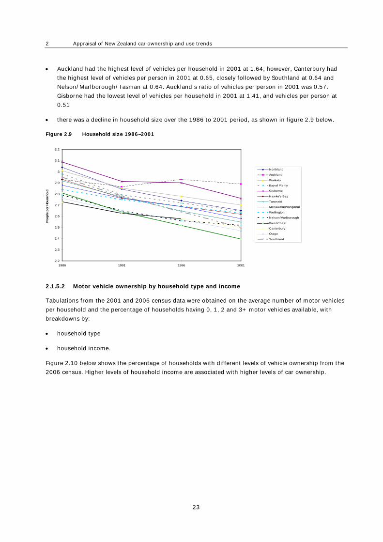
Auckland had the highest level of vehicles per household in 2001 at 1.64; however, Canterbury had
the highest level of vehicles per person in 2001 at 0.65, closely followed by Southland at 0.64 and
Nelson/Marlborough/Tasman at 0.64. Auckland’s ratio of vehicles per person in 2001 was 0.57.
Gisborne had the lowest level of vehicles per household in 2001 at 1.41, and vehicles per person at
0.51
there was a decline in household size over the 1986 to 2001 period, as shown in figure 2.9 below.
Figure 2.9 Household size 1986–2001
2.1.5.2 Motor vehicle ownership by household type and income
Tabulations from the 2001 and 2006 census data were obtained on the average number of motor vehicles
per household and the percentage of households having 0, 1, 2 and 3+ motor vehicles available, with
breakdowns by:
household type
household income.
Figure 2.10 below shows the percentage of households with different levels of vehicle ownership from the
2006 census. Higher levels of household income are associated with higher levels of car ownership.
2.2
2.3
2.4
2.5
2.6
2.7
2.8
2.9
3
3.1
3.2
1986 1991 1996 2001
Peo
ple
per
House
hold
Northland
Auckland
Waikato
Bay of Plenty
Gisborne
Hawke's Bay
Taranaki
Manawatu/Wanganui
Wellington
Nelson/Marlborough
West Coast
Canterbury
Otago
Southland

Development and application of a New Zealand car ownership and traffic forecasting model
24
Figure 2.10 2006 census – all family types
Other notable findings of the analysis included:
overall the average vehicles per household increased by a factor of over two from the lowest income
group (1.01 vehicles per household) to the highest income group (2.35 vehicles per household).
However, part of this increase might be ascribed to household size effects
households that contained a greater number of adults tended to have more vehicles per household:
- couples with dependent children averaged 1.94 vehicles per household
- couples averaged 1.79 vehicles per household
- single adult with dependent children averaged 1.07 vehicles per household
- single people averaged 0.90 vehicles per household
households that contained retired people tended to have a fewer vehicles per household:
- couples averaged 1.58 vehicles per household
- single people averaged 0.74 vehicles per household.
2.1.5.3 Reconciliation of census and national statistics
The census data potentially provides the best basis for forecasting motor vehicle ownership levels at the
regional level, or at more detailed levels (zonal or TLA): household number projections are available at the
regional and more detailed levels, and the census motor vehicle ownership data is household based.
However, the census data does not represent all motor vehicles: not only are motorcycles deliberately
excluded, but company-owned vehicles which are not kept at private residences overnight are excluded.
The TRC statistics are the official records for motor vehicle ownership, and the project vehicle ownership
time series is based on the TRC September quarterly returns. To enable estimates of motor vehicle
ownership to be made at the regional level from census data, it is necessary to reconcile the census data
with the TRC statistics (cars only).
0%10%20%30%40%50%60%70%80%90%
100%
Loss
- $1
0k
$10k
- $1
5k
$15k
- $2
0k
$20k
- $2
5k
$25k
- $3
0k
$30k
- $4
0k
$40k
- $5
0k
$50k
- $7
0k
$70k
- $1
00k
$100
k or
Mor
e
Household Income
% H
ouse
hold
s w
ith
3+ Vehicles
2 Vehicles
1 Vehicles
O Vehicles

2 Appraisal of New Zealand car ownership and use trends
25
An analysis was conducted of the differences between the 1991, 1996, 2001 and 2006 census and TRC
data (March 1991, 1996, 2001 and 2006). The results are set out in table 2.2 below. Overall the census
figures appear to be around 2%–6% higher than the adjusted TRC figures. The TRC figures are considered
to be more reliable than the census figures as they are based on actual transactions rather than survey
responses. There are differences in the definition of motor vehicles between the two data sets which could
explain some of the differences in ownership figures. The census data includes cars (licensed and
unlicensed) and vans, and could possibly include taxis, rental cars and some trucks. TRC data includes
licensed cars, rental cars, taxis and trade plates.
Table 2.2 Comparison of vehicles per person
Vehicles per person Vehicles per person – New Zealand
1991 1996 2001 2006
TRC(a) – original 0.459 0.469 0.504 0.550
– adjusted 0.482 0.493 0.529 0.577
Census(b) 0.492 0.521 0.544 0.586
Ratio – census: TRC adjusted 1.02 1.06 1.03 1.02
(a) TRC figures (March) – all cars, including rental cars and taxis
(b) Census figures – all vehicles used for personal use
2.2 New Zealand car use trends
This section details the various data that has been found on car use trends in New Zealand (ie the amount
of travel occurring).
2.2.1 New Zealand Household Travel Survey
The New Zealand Household Travel Survey is a survey of household travel conducted for the MoT.
The first survey was undertaken in the period July 1989 to June 1990 and surveyed some 4000 occupied
dwellings with 8700 responses received. The second survey was undertaken between June 1997 and July
1998 and surveyed some 7000 occupied dwellings with 14,000 responses received. The survey is now
undertaken continuously where people in over 2000 households throughout New Zealand are invited to
participate in the survey by recording all their travel over a two-day period. Data is available on the MoT
website for the period March 2003 to June 2006.
The following table summarises some of the data from the travel surveys. Table 2.3 also shows a
comparison in percentage change in car ownership. This comparison shows that driver travel has
increased at a similar rate as car ownership. Between 1989/90 and 2003/06 car ownership increased by
approximately 47.6% while driver travel increased by 45.1%. However, the number of driver trips increased
at a lower rate than car ownership. Between 1989/90 and 2003/06 car ownership increased by
approximately 47.6% while driver trips increased by 29.7%.

Development and application of a New Zealand car ownership and traffic forecasting model
26
Table 2.3 New Zealand Household Travel Survey: trips and travel
Year
1989/1990 1997/1998 2003/2006
Driver trips (millions) 2529 3093 3281
– % change since 89/90 – 22.3% 29.7%
Driver travel (100m km) 202 273 293
– % change since 89/90 – 35.4% 45.1%
Car ownership % change since 89/90 – 19.4% 47.6%
2.2.2 Ministry of Transport – warrant of fitness data
Information on vehicle kilometres travelled (VKT) was obtained from the MoT, based on odometer readings
taken as part of the warrant of fitness (WoF) programme. Table 2.4 summarises the VKT estimates while
figure 2.11 shows annual light vehicle travel per capita and figure 2.12 shows average annual travel per
vehicle. While the data is only available since 2001, the following trends have occurred:
light vehicle travel per capita increased between 2001 and 2005, but decreased in 2006
average annual travel per vehicle has been decreasing since 2002.
Table 2.4 WoF VKT estimates
Year Light travel per capita
(km)
Light travel per vehicle
(km)
2001 8481 13,073
2002 8592 13,131
2003 8680 13,014
2004 8793 12,883
2005 8790 12,562
2006 8615 12,232
Figure 2.11 Light fleet travel per capita
Source: MoT (2007)
7000
8000
9000
10000
2002 2003 2004 2005 2006
Period
An
nu
al K
m

2 Appraisal of New Zealand car ownership and use trends
27
Figure 2.12 Light fleet average annual travel per vehicle
Source: MoT (2007)
2.2.3 Traffic count data
MoT undertook counts at around 2300 locations in 2000, 2001, 2003 and 2005 for the purpose of
estimating car use, and as a proxy for car VKT. Traffic was counted for three hours per site and inflated to
estimate annual traffic for each site. This has now been discontinued in favour of the WoF data (see
section 2.3.2) which is deemed to be more reliable.
Figure 2.13 shows the estimate of total VKT in New Zealand, while figure 2.14 shows the breakdown by
region. As shown in figure 2.13, the estimates derived from the traffic counts follow the same trend as
those derived from WoF data, although they are 1% – 3% higher. Figure 2.14 shows that Auckland (which is
home to 32% of the national population) contributes to approximately 28% of New Zealand’s VKT.
Figure 2.13 Vehicle travel method comparison
11,000
11,500
12,000
12,500
13,000
13,500
2002 2003 2004 2005 2006
Period
An
nu
al K
m p
er v
ehic
le
30.0
32.0
34.0
36.0
38.0
40.0
42.0
2000 2001 2002 2003 2004 2005
Year
Veh
icle
Km
Tra
vel
(Bil
lio
n V
KT
)
Traff ic CountEstimateWoF

Development and application of a New Zealand car ownership and traffic forecasting model
28
Figure 2.14 Vehicle travel by region
Traffic count data was also obtained from Transit NZ (now NZTA) from their Auckland continuous
motorway count programme. Average daily traffic (ADT) estimates from 19 count sites were provided for
2001 to 2006. Figure 2.15 shows the total ADT across the 19 count sites. The trend is generally similar to
the WoF data (figure 2.11) which shows increasing travel up to 2005 and then a decline in 2006.
Figure 2.15 Sample Auckland Transit NZ traffic counts
2.2.4 Regional household interview surveys
Larger regional councils conduct household interview surveys as part of their transport modelling
programmes. These surveys capture information relating to household characteristics and trip-making
behaviour (through the use of trip diaries).
Auckland has recently completed surveys as part of their ATM2 model development. The survey sampled
some 10,000 households in 2006, of which final responses were received from 6000 households. Key
information collected includes:
1,420
1,440
1,460
1,480
1,500
1,520
1,540
1,560
1,580
2001 2002 2003 2004 2005 2006
Year
AD
T (
Th
osa
nd
s)
-
2.0
4.0
6.0
8.0
10.0
12.0
2000 2001 2002 2003 2004 2005
Year
Veh
icle
Km
Tra
vel
( B
illi
on
VK
T) Auckland
Waikato
Canterbury
Wellington
Manaw atu.Wanganui
Otago
Bay of Plenty
Northland
Haw kes Bay
Nelson.Marlborough
Southland
Taranaki
West Coast
Gisborne

2 Appraisal of New Zealand car ownership and use trends
29
number of residents in household
age of people
employment status
type of vehicle
travel information including:
- trip purpose
- mode of transport
- driver or passenger.
As these surveys are undertaken relatively infrequently they are of limited value in determining trends.
2.2.5 Impacts of transport fuel price changes
Booz Allen Hamilton (2007) undertook research to assess evidence on the impacts of petrol price changes
on New Zealand petrol consumption, traffic volume and public transport patronage; and, in the light of
this evidence and evidence from Australia and other countries, to recommend a set of ‘best estimate’
petrol price elasticities in the New Zealand context. The research was completed in 2007 and published as
Land Transport NZ research report 331.
Figure 2.16 shows changes in petrol consumption (per person per day) as the petrol price index changed
over the period 1978–2006. Both data sets were smoothed with four-quarter-moving averages. It appears
that for most of the period analysed, petrol consumption trends ‘mirrored’ petrol price trends, ie
increased petrol price resulted in less fuel consumption per person per day.
Figure 2.16 Trends in petrol prices and petrol consumption (1978–2006)
Source: Booz Allen Hamilton (2007)
Petrol Consumption per Person per Day
Petrol Index
1.2
1.3
1.4
1.5
1.6
1.7
1.8
1978
1979
1980
1981
1982
1983
1984
1985
1986
1987
1988
1989
1990
1991
1992
1993
1994
1995
1996
1997
1998
1999
2000
2001
2002
2003
2004
2005
2006
Co
nsu
mp
tio
n o
f P
etro
l per
Per
son
per
Day
0
0.5
1
1.5
2
2.5
Pet
rol P
rice
Ind
ex(S
cale
d t
o t
he
Mar
-20
06 N
Z P
rice
of
Reg
ula
r P
etro
l)

Development and application of a New Zealand car ownership and traffic forecasting model
30
Figure 2.17 shows the percentage change in total traffic volumes (per capita), petrol prices and GDP per
capita. Throughout the period until mid-2005, car traffic volumes per capita increased continuously,
generally at a rate of around 1% – 2% per year; since then, car volume trends have become negative, with
the latest (mid-2006) data indicating an annual decline of 4% – 5%. The study suggested there was a
relationship between traffic volumes and petrol prices, particularly in the periods around July 2003, April
2005 and since October 2005.
Figure 2.17 Changes in total traffic volume per capita, petrol price and GDP per capita
2.3 Comparison with international data
There is generally a wide range of international data available on car and vehicle ownership. However, due
to differences in definitions and years where data is available, it is difficult to produce a consistent time
series of data.
The Organisation for Economic Cooperation and Development (OECD) has produced vehicle ownership
rates for a large set of countries between 1990 and 2004 based on available data. Figure 2.18 shows that
New Zealand had amongst the highest vehicle ownership in the world (note this data includes all vehicles
such as trucks and buses). Most countries showed an upward trend in vehicle ownership between 1990
and 2005. The notable exception was the United States, which although it had decreased vehicle
ownership since 1990, still had the highest rate of vehicle ownership of the OECD data.
Transfund NZ research report 161 (Booz Allen Hamilton 2000) contained a figure showing car ownership
between 1958 and 1988 for New Zealand, United States, United Kingdom, Canada and Victoria. Until
1988, New Zealand car ownership had closely matched that of Canada. However, as shown in figure 2.18,
in the period 1990–2005, Canada’s vehicle ownership decreased while New Zealand’s continued to
increase.
Price of Regular Petrol
GDP per Capita
-0.1
-0.05
0
0.05
0.1
0.15
0.2
0.25
Jan-03 Apr-03 Jul-03 Oct-03 Jan-04 Apr-04 Jul-04 Oct-04 Jan-05 Apr-05 Jul-05 Oct-05 Jan-06 Apr-06
(13-
Mon
th M
ovin
g A
vera
ges
of)
Per
cent
age
Cha
nges
Traffic Volume per Capita

2 Appraisal of New Zealand car ownership and use trends
31
Figure 2.18 International vehicle ownership comparison
Source: OECD Factbook 2006 – selected countries
Figure 2.19 below shows a comparison of vehicle ownership rates, produced by MoT based on 2002 data.
Again, it can be seen New Zealand, in that year, had one of the highest vehicle ownership rates in the world.
Figure 2.19 Vehicles per 1000 population (as at 2002)
Source: MoT (2007)
0
100
200
300
400
500
600
700
800
900
1990 1995 2000 2005Year
Veh
icle
s P
er T
ho
usa
nd
Peo
ple
United States
Portugal
Luxembourg
New Zealand
Italy
Australia
Japan
France
Canada
United Kingdom
Sw eden
Ireland
Denmark
Korea
Russian Federation
200 300 400 500 600 700 800
BELGIUM
FRANCE
MALTA
AUSTRIA
SWITZERLAND
AUSTRALIA
GERMANY
PORTUGAL
CANADA
ICELAND
ITALY
ANDORRA
LUXEMBOURG
NEW ZEALAND
LIECHTENSTEIN
USA (*)

Development and application of a New Zealand car ownership and traffic forecasting model
32
2.4 Conclusions
Examination of New Zealand car ownership and use data shows the following:
Car ownership has continued to increase. In 1970 car ownership was 0.310 cars per person; by 2005
it had risen to 0.574 cars per person.
There appears to be a relationship between times of increasing GDP per person and decreasing car
prices corresponding to increased car ownership per person.
New Zealand continues to have one of the highest rates of car ownership in the world.
The census data provides the best basis for comparing car ownership between regions.
The most comprehensive set of data on car use in New Zealand is the MoT New Zealand Household
Travel Survey. This survey has been undertaken continuously since 2003 and shows that since about
1990, driver travel has increased at approximately the same rate as car ownership (approximately 45%).
Information on VKT has been collected since 2001, using odometer readings taken during the vehicle
WoF inspections. This data shows that light vehicle travel per person increased between 2001 and
2005, but decreased in 2006. Average annual travel per vehicle has been decreasing since 2002.
Previous research showed that higher petrol prices resulted in less fuel consumption per person.
Regarding the data itself, the following conclusions have been reached:
Due to changes in motor vehicle registration processes, there is some difficulty in determining
accurate vehicle ownership in New Zealand, particularly a time series of data. This highlights the
importance of collecting ongoing data in a consistent manner.
There are different definitions used for car ownership levels. For example census data is not directly
comparable to TRC figures due to the different definitions. It would be beneficial if these definitions
could be brought into line or segregated to enable direction comparisons.

3 Update of a New Zealand aggregate car ownership model
33
3 Update of a New Zealand aggregate car ownership model
3.1 The Booz aggregate car ownership model
3.1.1 Introduction
Booz Allen Hamilton (2000) previously developed an aggregate model for forecasting future car
ownership. This section builds on the previous work and updates the model using latest data and research
(note the previous research was based on data up to 1996). The approach adopted was a macro-economic
model that estimates car ownership at a national level. See section 6 for the background to the selection
of this model.
3.1.2 Basis for forecasting vehicle ownership
There are two critical elements in providing realistic vehicle ownership forecasts in macro-economic
(aggregate time series) models:
the growth path to saturation
the saturation level.
A number of different methods have been used to predict these two elements. Most have used ‘s-curves’
to model the growth path to saturation. In New Zealand, both MoT (as part of the vehicle fleet emissions
model work) and Beca (2003) have used logistic form s-curves. These models assume a constant or fixed
saturation level. By contrast, the previous Booz Allen Hamilton (2000) research used a changing saturation
level, (reflecting changing demographics) but a more simplistic growth path to saturation. This approach
was adopted for this research.
3.1.3 Saturation level
The saturation level of car ownership per capita is unclear and there appears to be considerable variation in the
assumptions used in forecasting it. Two approaches are normally adopted to estimate the saturation level:
use of statistical techniques on existing data to extrapolate a growth path: the saturation level is
taken where this growth path levels off
examination of the behaviour of the car-owning population with relatively high incomes: saturation
levels estimated for this population are assumed to flow through to the remaining population of car
owners as their real income levels increase over time.
The first of these approaches to forecasting a saturation level involves fitting a regression line to the
annual growth rates of per capita car ownership, and extrapolating this line to the x axis. However, this
approach fails to address the effect of economic influences (eg income, real cost of motoring) on the
growth path. The development of a saturation level is a long-term effect and there is considerable
uncertainty that the modelled relationship would continue to hold in the long term, even when economic
influences are included in the model.

Development and application of a New Zealand car ownership and traffic forecasting model
34
The second approach to forecasting car ownership looks at the behaviour of the car-owning population
with relatively high incomes. This is considered a more sensible approach as economic influences have
been shown to be a key determinant in car ownership.
It is also noted, and needs to be taken into account, that the saturation level of car ownership per capita
will be influenced by the following factors:
the proportion of the population who are permitted by law to drive
the proportion of the potential car-owning population unable to drive because of physical or mental
disability
the proportion of the potential car-owning population who choose not to own a car.
3.1.3.1 New Zealand data and references
New Zealand census data for 2006 was reviewed and tabulations were obtained for car ownership (0, 1, 2
and 3+ cars), household structure and household income. The following key points were identified:
Considering single adult households:
- 77% own at least one vehicle
- 94% with an income over $50,000 own at least one vehicle
Considering households of couples:
- 65% own at least two vehicles (ie an average of at least one vehicle per adult)
- 80% with a household income over $70,000 own at least two vehicles
- 82% with a household income over $100,000 own at least two vehicles
Considering households of couples with dependent children:
- 75% own at least two vehicles (ie an average of at least one vehicle per adult)
- 85% with a household income over $70,000 own at least two vehicles
- 88% with a household income over $100,000 own at least two vehicles
This data suggests that a saturation level of car ownership of high-income adults in New Zealand could be
between 80% (high-income couples) and 94% (high-income single adults). It is important to note that the
above data is based on proportions of households that owned at least X vehicles, as opposed to average
number of vehicles. This is because some household types averaged more cars than adults (this is
discussed later in this section). For example, high-income single-person households averaged over one
car per household.
Another source of information is the proportion of the population with a current driver licence. It is
hypothesised that the saturation level could be everyone who has a licence would like to own a car, should
income allow.
Data was obtained from the NZTA on the number of driver licences held, categorised by age and gender
(as at the end of 2007). The following key points were identified:

3 Update of a New Zealand aggregate car ownership model
35
approximately 96% of the population aged between 15 and 65 have a driver licence
approximately 76% of the population aged over 65 have a driver licence
overall approximately 93% of the population aged over 15 have a driver licence or 74% of the total
population
assuming the current licence rates continue and with the projections for an aging population in
New Zealand, in 2041 approximately 77% of the total population will have a driver licence.
It is noted that Beca (2003) adopted a saturation rate of 0.75 cars per capita (ie 75% of the total
population) based on analysis of current and future licence holdings. By comparison the MoT VFEM uses a
saturation rate of 0.65 cars per capita (see section 5).
3.1.3.2 Australian data and references
Beca (2003) reported that the Australian BTRE had raised its saturation level expectation to around 0.65 cars
per capita. Booz Allen Hamilton (2000) reported that in Australia, about 5% of the potential car-owning
population were unable to use a car because of disability, mainly because of advanced age or poor eyesight.
3.1.3.3 United Kingdom data and references
As cited in Booz Allen Hamilton (2000), the UK national road traffic forecasts (NRTF) model assumed a
saturation level based on cars being owned by 90% of the driving age group, defined as 17–74 year olds.
3.1.3.4 United States data and references
Booz Allen Hamilton (2000) analysed historical data from the United States. Key findings of this data included:
the ratio of cars to driving licences for the three states with the highest levels of car ownership in
1986 varied from 1.01 (Florida) to 1.13 (New Hampshire)
US National Transportation Personnel Study data showed a levelling off at around 0.95 cars per adult
at relatively high income levels.
3.1.3.5 Other comments
An initial plausible assessment is that the saturation level will occur when every person of driving age
owns a car, with the exception of those who have a disability that prevents them from driving. However,
the United States data, which indicates more cars than driving licences in some states and New Zealand
census data which shows some household and income levels have more cars than adults, casts some
doubt on whether this is really the saturation level of ownership: as cars get relatively cheaper to own,
affluent people may well own more than one car, using different car types for different types of trips.
However, in cases where households have more cars than licence holders, not all the cars can be in use
simultaneously and the marginal cars are unlikely to result in substantial increase in vehicle kilometres
travelled. Hence for traffic planning purposes, it may be reasonable to estimate the ‘effective’ saturation
level on this basis, while recognising that the physical saturation level may be higher.
The proportion of the potential car-owning population who choose not to own a car will vary depending
on location. Vehicle ownership in major urban areas such as London, Tokyo and New York, is lower than in
smaller cities and rural areas. However, much of this is due to physical constraints on car ownership and
use, particularly congestion and parking problems. The effect of public transport provision on car

Development and application of a New Zealand car ownership and traffic forecasting model
36
ownership levels in New Zealand was investigated by Booz Allen Hamilton (2000) and concluded to be
equivalent to around -0.05 (-5%) vehicles per capita at current levels, based on United Kingdom, European
and Australian analysis.
3.1.3.6 Adopted saturation level
The following table summarises the above discussion on saturation rates.
Table 3.1 Summarised sources of possible saturation rates
Source Effective cars/
adult(a)
Effective cars/
capita
Comments
Booz Allen Hamilton: NZ
census
80% – 94% 63% – 74% Based on analysis of high-income
singles and couples
Booz Allen Hamilton: NZ
driver licence
93% 74% Percentage of population that has a
current driver licence
Beca (2003) - 75% Based on analysis of New Zealand
driver licence data
MoT VFEM - 65% Unknown basis
BRTE Forecasts – Australia - 65% Cited in Beca (2003)
UK NFTF model 90% - Cited in Booz Allen Hamilton (2000)
USA data 95% - Cited in Booz Allen Hamilton (2000)
(a) Person of driving age (in the New Zealand context this means persons 15 years or older)
Based on the above data and research, we propose the following range of saturation levels:
likely upper saturation: 0.95 ‘effective’ cars per adult (person of driving age)
likely saturation: 0.90 ‘effective’ cars per adult
likely lower saturation: 0.85 ‘effective’ cars per adult.
Based on the current (2008) New Zealand population profile this results in:
likely upper saturation: 0.75 ‘effective’ cars per capita
likely saturation: 0.71 ‘effective’ cars per capita
likely lower saturation: 0.67 ‘effective’ cars per capita.
The above likely saturation rates, relating to cars per driving-age population, appear to be broadly
consistent with other cited experience and data. For example, with a starting point of 100% of the driving
age population, the following reductions can be applied:
A proportion of the driving age population will be unable to use a car because of disability. Some
Australian data suggests this could be approximately 5% of the potential car-owning population.
In practice, there will always be a proportion of the population who choose not to own a car (apart
from reasons of disability etc). Based on United Kingdom experience, this could be approximately 5%
of people of driving age.

3 Update of a New Zealand aggregate car ownership model
37
In addition, in urban areas car ownership levels are likely to be lower due to the availability of public
transport and the constraints on car use (car parking limitations etc). This might reduce saturation
levels by a further 5% of the people of driving age.
Table 3.2 shows the projected distribution of population in New Zealand by age group and the
corresponding maximum and minimum saturation levels per capita (assuming that the minimum driving
age is retained at 15). It indicates gradual increases in saturation levels over time, as the proportion of
children in the population is predicted to decrease. The current saturation levels are in the range 0.67 cars
per capita (lower) to 0.75 cars per capita (upper). By year 2041 these increase, due to changes in age
distribution, to 0.71 cars per capita (lower) and 0.79 cars per capita (upper).
Table 3.2 New Zealand population distribution and car ownership saturation levels
% Population by age Saturation level
(cars/capita)
Year 0–14 15–64 65+ Lower(a) Upper(b)
1996 23.0 65.4 11.5 0.654 0.731
2001 22.6 65.5 11.9 0.658 0.735
2006 21.2 66.5 12.2 0.670 0.748
2011 20.4 66.3 13.3 0.677 0.756
2021 19.2 63.6 17.1 0.686 0.767
2031 17.7 60.8 21.4 0.699 0.781
2041 17.0 59.2 23.9 0.706 0.789
Source: Statistics NZ ‘New Zealand Population Projections’ 2006 (base) – 2061 – Series 5 base
(a) Lower = 0.85 cars/capita of age 15+
(b) Upper = 0.95 cars/capita of age 15+
While it may appear confusing to have a saturation level that changes over time (when defined in terms of
cars per capita), this is simply reflecting the changing proportion of the population that are of driving age.
The saturation level, as defined in terms of cars per adult, is fixed and is not proposed to change over
time.
3.1.4 Growth to saturation
The second element in forecasting future car ownership levels is the growth path taken to reach the
saturation level. Key influences include:
general level of economic activity (normally measured in GDP per capita)
real cost of motoring (both car purchase and car use)
household structure
relative accessibility of private and public transport consumer taste.
As identified by Booz Allen Hamilton (2000), the evidence from many countries and from New Zealand data
up to 1970 was that the ‘underlying time trend’ had been the major factor determining trends in car
ownership; with growth in cars per capita being more or less linear and showing little signs of tailing off
towards saturation. Relatively small variations from the linear trend line were related to variations in income

Development and application of a New Zealand car ownership and traffic forecasting model
38
levels and motoring costs. However, analysis of New Zealand data since 1970 suggests that the apparent
‘unexplained’ time trend has reduced. With this reducing time trend, the effects from the trend of changes in
GDP and the car price index (new and used) have become relatively more significant.
The approach adopted to determine the likely growth path to saturation was to make a range of
projections based on multiple regression analysis of more recent New Zealand data and a range of
estimates for future trends in GDP per capita, the car price index1 and time trends.
Using the same method previously adopted by Booz Allen Hamilton (2000), two multiple linear regressions
were undertaken to further examine the relationship between the three-year moving average statistics for
annual percentage changes:
Regression (A): Cars/capita against GDP/capita and car price index
Regression (B): Cars/capita against GDP/capita, car price index and time.
Figure 3.1 shows the three-year moving average in cars per capita, GDP per capita and the car price index.
Figure 3.1 Three-year change in cars per person, GDP per person and car prices 1973–2006
It was found that regression (A) provided little or no explanation of the trend in cars per capita (r2 =
0.15). Regression (B) provided an improved fit (r2 =0.64), indicating a decrease in the annual time trend
over the period. The results for regression (B) are summarised in table 3.3. All three variables are
statistically significant to a 95% confidence level (using t test).
Table 3.3 Regression analysis results
Yearly time trend -0.001
Elasticity of cars/capita with GDP/capita + 0.52
Elasticity of cars/capita with the car price index - 0.18
The above regression analysis provided elasticities for GDP per capita and car prices per capita with
respect to car ownership. This regression analysis also identified a downward time trend. However the
1 The car price index incorporates new and second-hand car prices. It is noted that a better index would also
incorporate other car ownership costs.
-12.0%
-10.0%
-8.0%
-6.0%
-4.0%
-2.0%
0.0%
2.0%
4.0%
6.0%
8.0%
1973 1975 1977 1979 1981 1983 1985 1987 1989 1991 1993 1995 1997 1999 2001 2003 2005
Ave
rag
e A
nn
ual
Per
cen
tag
e C
han
ge
Cars/Psn
GDP/Psn
Car Prices

3 Update of a New Zealand aggregate car ownership model
39
linear regression equation developed (B) did not take into account that the time trend would eventually
reach zero. Therefore, the time trend component of regression (B) was modified to provide the following
predictive equation:
Regression (C) = Cars/capita against GDP/capita, car price index and reducing time trend.
or
% change in cars/capita = % change in GDP/capita * GDP elasticity + % change in car price index * car price index elasticity + time trend for year X (if greater than 0)
The reducing time trend component of the equation consists of a starting percentage (at 1973) and a
yearly reduction. Using the data set from 1973 to 2006 and the ‘least squares’ method to solve the
equation, the starting percentage and yearly reduction were found to be:
2.6% starting percentage in 1973, reducing by 0.13% per year to reach a 0% time trend in 1993.
This indicates that changes in car ownership in New Zealand are no longer influenced by the unexplained
time trend.
Therefore the final form of the regression (C) equation is:
% change in cars/capita = % change in GDP/capita x 0.52 (Equation 3.1)
+ % change in car price index x (-) 018
+ 2.6% - (year-1973) x 0.13% {only included if positive}
The resulting regression (C) has an improved r2 of 0.71 compared with an r2 of 0.64 for regression (B).
Figure 3.2 shows the actual cars per capita and modelled cars per capita. As shown the reducing time
trend model (regression (C)) performs well when compared with regression (B) and the actual data.
Figure 3.2 Regression of three-year moving average of changes in real GDP/person and real car price against
cars/person 1973–2006
-0.5%
0.0%
0.5%
1.0%
1.5%
2.0%
2.5%
3.0%
3.5%
4.0%
4.5%
5.0%
1973 1975 1977 1979 1981 1983 1985 1987 1989 1991 1993 1995 1997 1999 2001 2003 2005
Av
era
ge
An
nu
al P
erc
en
tag
e C
han
ge
Actual
Regression (B)
Regression (C) Reducingtime trend model

Development and application of a New Zealand car ownership and traffic forecasting model
40
3.1.5 New Zealand car ownership forecasts
The approach described above has been applied to developing a series of national New Zealand forecasts
of car ownership per capita on the following basis:
starting from the 2006 estimate of cars per capita, from the TRC figures, as adjusted (0.577 cars per
capita)
application of ‘low’, ‘medium’ and ‘high’ growth projections based on published forecasts for GDP and
the regression analyses undertaken and plausible ranges for trends in GDP per capita and car price
constraint of the ‘low’ and ‘high’ saturation levels as defined earlier.
Table 3.4 shows the inputs to the three sets of growth projections.
Table 3.4 Inputs to growth projections
Annual change % Input
Low growth Medium growth High growth
GDP/capita(a) + 0.5 + 1.5 + 2.0
Car price index +0.5 0.0 -1.0
(a)Between 2007 and 2012 the actual Treasury forecasts for GDP/capita growth have been used (for all three scenarios).
The Half year economic & fiscal update 2007, produced by the Treasury, provides forecasts for GDP
growth per capita until 2012. The forecast growth ranges from +0.5% to +2.0% with an average of +1.5%.
By way of comparison, over the 36-year period 1970–2006 GDP per capita grew on average +1.8% per
year.
Over the 36-year period 1970–2006 car prices fell on average by 1.1% per year. However, the decline in
car prices is unlikely to continue at this rate for the following reasons:
Some of the reduction of real car prices has been the result of one-off changes, such as the removal
of import tariffs.
The government has recently imposed stricter rules on the maximum age of imported vehicles,
meaning that imported Japanese vehicles could be more expensive in the future.
Growing environmental awareness is likely to lead to tougher standards and new technologies being
required for vehicles, which could result in higher car production costs. With higher oil prices, as well
as growing environmental awareness, there will be greater development of alternative fuel source
vehicles (rather than the cheaper refinement of the existing petrol engine).
Based on these projections and the 2006 car ownership level, table 3.5 and figure 3.3 show projected car
ownership levels up to year 2041, indicating that economic conditions and car prices are predicted to have
a significant bearing on future car ownership.
Under these estimates, if growth were to continue according to the projections shown, eventually the
postulated saturation levels would be reached. For instance, the ‘high growth’ projection line reaches the
lower saturation level in about 2021 and the higher saturation level in about 2031.

3 Update of a New Zealand aggregate car ownership model
41
The Booz aggregate model is based on using developed elasticities to predict the change in car ownership.
A disadvantage with this model form is that it does not model the ‘tailing off’ that might be expected prior
to reaching saturation levels (as happens when an s-curve is used). In practice, therefore, while not shown
in figure 3.3, a tailing off of growth for these projections is expected prior to the reaching of saturation
levels. However some researchers (eg Romilly et al 1998) have argued that car ownership does not form a
s-curve type trend in any event.
Table 3.5 Estimates of cars per capita to 2041
Year Low growth Medium growth High growth
2006 0.577 0.577 0.577
2011 0.596 0.599 0.604
2016 0.606 0.625 0.643
2021 0.611 0.649 0.683
2026 0.617 0.675 0.726
2031 0.622 0.702 0.772
2041 0.633 0.760 0.789*
* Capped at the high estimate of saturation
Figure 3.3 Estimates of car ownership in New Zealand until 2041
3.2 Comparison with other New Zealand model forms
The Booz aggregate model described above has been compared with the two other model forms adopted
in New Zealand:
the vehicle fleet emissions model (VFEM) car ownership equation (MoT)
the Tauranga transportation model (TTM) car ownership equation (Beca).
0
0.1
0.2
0.3
0.4
0.5
0.6
0.7
0.8
1970
1973
1976
1979
1982
1985
1988
1991
1994
1997
2000
2003
2006
2009
2012
2015
2018
2021
2024
2027
2030
2033
2036
2039
2042
Year
Car
s Per
Per
son
Pre 1986
Post 1986
Likely Lower Saturation
Likely Upper Saturation
Low Estimate
Medium Estimate
High Estimate

Development and application of a New Zealand car ownership and traffic forecasting model
42
The forms of these models are as follows.
VFEM car ownership model:
(Equation 3.2)
where:
t = the year
a and b = constants
S = saturation level of car ownership
TTM car ownership model:
(Equation 3.3)
where:
T = the year (eg 2007)
G = GDP/capita
CP = index of car prices
a, b, c and d = constants
S = saturation level of car ownership
The above models have been re-calibrated using the same data as used for the Booz aggregate model and
adopting the same upper saturation ratio of 0.789 (in 2041).
Figure 3.4 shows the predictions from these equations compared against the aggregate elasticity model.
As shown in this figure, the three models perform in a similar manner between 2007 and 2030
(approximately). Beyond 2030 the Booz aggregate model has a higher car ownership rate as it does not
model the ‘tailing off’ that is expected to occur as car ownership approaches saturation.
Figure 3.4 Comparison of equations against aggregate elasticity model
0
0.1
0.2
0.3
0.4
0.5
0.6
0.7
0.8
1970
1973
1976
1979
1982
1985
1988
1991
1994
1997
2000
2003
2006
2009
2012
2015
2018
2021
2024
2027
2030
2033
2036
2039
2042
Year
Cars
Per
Pers
on
Pre 1986
Post 1986
Likely Lower Saturation
Likely Upper Saturation
Medium Estimate
TTM Model
VFEM
/(1 . )a bt
Scars head
e e
./
1 . b T c d
Scars head
a e G CP

3 Update of a New Zealand aggregate car ownership model
43
3.2.1 Prediction comparison: 1997–2006
In order to compare the performance of the three models, particularly in the short term, the three models
were re-calibrated using data from 1970 to 1996. The predictions from these models for the 10-year
period between 1997 and 2006 (inclusive) were then compared against actual car ownership data. The
results are shown in figure 3.5 below. As shown, all three models appear to provide reasonable estimates
of car ownership over the relatively short-term 10-year period. However, the Booz aggregate model more
closely replicates the trend in car ownership over this period.
Figure 3.5 Comparison of model predictions 1997–2006
3.3 Conclusions
The following key conclusions have been made from the results presented in this section.
The current level of car ownership in New Zealand, approximately 0.58 cars per capita, is below the
estimated saturation level of car ownership. The current saturation levels are estimated to be in the
range 0.67 cars per capita (lower) to 0.75 cars per capita (upper). By year 2041 the saturation level is
predicted to increase, due to changes in age distribution, to between 0.71 cars per capita (lower) and
0.79 cars per capita (upper).
Elasticities of GDP per capita and car price index can be used to predict future changes in car
ownership (Booz aggregate elasticity model), particularly in the short to medium term. These appear
to be a strong set of relationships.
Using the Booz aggregate model under the ‘high’ scenario, car ownership could reach the lower
estimate of saturation by approximately 2021.
The aggregate elasticity model appears to perform better than the other examined aggregate models
in the short-term (< 10 years). Over the medium term (10–20 years) the three models perform in a
similar manner. In the longer term (>20 years) it is likely that the aggregate elasticity model will not
perform as well as the other model types as it cannot replicate the ‘tailing off’ of car ownership
growth that is likely to occur as saturation is approached
Economic conditions and car prices are predicted to have a significant impact on future car ownership.
0.4
0.5
0.6
1987
1990
1993
1996
1999
2002
2005
Year
Car
s P
er P
erso
n
Recorded Data
Booz Aggreate Model
TTM Model
VFEM Model

Development and application of a New Zealand car ownership and traffic forecasting model
44
There is considerable uncertainty over factors that could have a significant impact on car ownership. For
example it is unlikely that the real downward trend in the car price index will continue. The ability to
forecast future car ownership is dependent on the ability to accurately forecast changes in GDP and car
prices.

4 Development of policy and functional requirements
45
4 Development of policy and functional requirements
4.1 Car ownership and use ‘needs’ survey
A survey was developed as part of the scoping for this project to examine current and future uses of car
ownership and use data, current sources of such data and possible features that might be included in the
development of a New Zealand modelling methodology.
Members of the steering group and peer reviewers were given the opportunity to comment on the survey,
with their suggestions being adopted by the study team.
The survey was distributed by email, and respondents were given around three weeks to reply. By the end
of the allotted timeframe only 50% of the final sample had been returned and so respondents were given
the opportunity to respond within the following week.
Responses were collated within a spreadsheet, and various statistics were developed.
4.1.1 Respondents
The survey was initially sent out to 26 individuals from 16 organisations. Two suggestions were made by
the peer reviewers: the first was to include consultancies within the sample, and as such five consultancies
were contacted; the second was to include Australian practitioners; however, it was felt that given this was
a New Zealand needs survey Australian views would add little.
It was made clear in the survey preamble that the views given by the respondents were to be taken as their
individual views, and not necessarily the views of the organisation they represented. As such, the
conclusions drawn from this survey do not necessarily reflect organisational needs.
Where the survey was sent to a number of respondents within the same organisation, some respondents
decided to pool responses together as one. By the end of the survey window, 17 responses were obtained
representing the view of 22 individuals from 15 organisations. The following organisations took part in
the survey:
Land Transport NZ
Ministry of Transport
Transit NZ
Ministry of Economic Development
The Treasury
Automobile Association
Auckland Regional Transport Authority
Auckland Regional Council

Development and application of a New Zealand car ownership and traffic forecasting model
46
Greater Wellington Regional Council
Christchurch City Council
five consultancies.
4.2 Survey results
4.2.1 Current sources of car ownership and use data
Respondents were asked to list their current sources of historical and forecast data for car ownership and
use. The responses have been categorised into broad sources, with the number of times the source
mentioned recorded. Note that many respondents recorded more than one source for their car ownership
and use data. The top five sources are shaded.
Table 4.1 Sources of car ownership and use data
Source Number of times
recorded
Percentage of
responses
Statistics New Zealand (including census) 12 71%
Transport Registry Centre 5 29%
Regional household travel survey 5 29%
Third party publications 4 24%
Transport models 4 24%
Traffic count data 3 18%
Ministry of Transport HH travel survey 2 12%
Motor Industry Association (MIA) 1 6%
Membership data 1 6%
Fuel sales/road user charges (RUC) 1 6%
The most significant source for car ownership and use data was Statistics NZ, and in particular its census
car ownership data (journey to work data was also mentioned). Motor vehicle registration data and
regional household travel surveys were also frequently mentioned. Transport models (such as the VFEM
and regional transport models) were mentioned by four practitioners, while others referred to third party
publications for source data. It should be noted that transport model outputs are in effect a secondary
data source as they are built on other data sources.
4.2.2 Current uses of car ownership data
Respondents were asked to list their current uses of car ownership and use statistics. Many of the answers
were varied, and as such were allocated into broad categories of usage. There were significant overlaps
between categories; for example, many respondents used car ownership data in transport models, but
these models were in turn used to provide inputs into funding, policy, planning and monitoring functions.

4 Development of policy and functional requirements
47
Table 4.2 Current uses of car ownership data
Current uses Number of times
recorded
Percentage of
responses
Policy analysis 10 59%
Transport models 7 41%
Evaluation 3 18%
Funding/value for money 2 12%
Project planning 2 12%
Monitoring 2 12%
The three most stated uses of car ownership and use data were for policy analysis, and for use in
transport models and in project evaluation.
4.2.3 Future uses of car ownership data
Respondents were asked what their future uses of car ownership and use data would be if there was a
source that met their needs. A certain amount of interpretation of the responses has been undertaken by
the researcher to categorise them into broad themes.
Table 4.3 Future uses of car ownership data
Future uses Number of times
recorded
Percentage of
responses
No change in requirement 8 47%
Improve/update transport models 3 18%
Improve spatial understanding 3 18%
Better understanding of usage drivers 2 12%
Impact of new technologies 2 12%
Impact of changes in fleet mix 2 12%
Improve performance monitoring 1 6%
For many, the current data sources met their anticipated future needs. Some responses highlighted better
data as a source for improving and updating transport models. Others mentioned the identification of
spatial (geographical) differences as a potential future use of an improved modelling methodology.
4.2.4 Potential features of future car ownership model
Respondents were asked to provide a priority ranking for potential features of a car ownership and use
model. These features were grouped into the following categories:
modes
level of geographic context
forecasting horizon
vehicle characteristics

Development and application of a New Zealand car ownership and traffic forecasting model
48
policy measures
possible outputs
other features not included in this list.
Rankings were given for ‘not relevant’, low, medium and high priorities, and converted into scores using a
scale 0 (not relevant) to 3 (high priority). Respondents were also given the opportunity to comment further.
Average scores have been provided for each feature, with those obtaining a score higher than 2 (on
average, better than medium priority) shaded. Variations in response scores are also provided (standard
deviation) to indicate a large variety of priority views between respondents.
4.2.4.1 Modes
Respondents were asked to provide a priority ranking for private cars, motorcycles and light commercial
vehicles (LCVs). Almost all respondents gave private cars a high ranking, with many giving the same
ranking to LCVs. Motorcycles were seen as less of a priority and, as one respondent put it ‘are only of
interest when considering safety issues’. Respondents suggested there should be a clear distinction
between private and company-owned cars (available for private use). Heavy commercial vehicles were also
mentioned; however, they are outside the scope of this study.
Table 4.4 Priority modes
Modes Average response Variation in response
Private car 2.94 0.24
Light commercial vehicle 2.47 0.72
Motorcycle 1.47 0.72
Private vehicles (including segmentation into private and company ownership) and LCVs are an important
part of a car ownership forecasting methodology.
4.2.4.2 Geography
Respondents were asked to provide a priority ranking for the geographical scope of a car ownership
forecasting methodology. Car ownership at a regional level had the highest ranking and most consistent
level of responses, and at a local level the lowest ranking and largest variation.
Table 4.5 Priority geography
Geography Average response Variation in response
National 2.41 0.87
Regional 2.71 0.47
Local 2.29 0.99
All geographic contexts had a high score, highlighting that any car ownership methodology would need to
have the ability to be applied at all spatial levels.
4.2.4.3 Forecasting horizon
Respondents were asked to provide a priority ranking of the forecasting horizons important to them.
Forecasting within the next 25 years was clearly the most important timeframe, with 5/10/25 years all

4 Development of policy and functional requirements
49
providing scores significantly greater than 2. Forecasting out to 50 years received a more mixed priority
ranking, with some respondents highlighting the significant amount of uncertainty associated with this
timeframe.
Table 4.6 Priority forecast horizon
Horizon Average response Variation in response
5 years 2.56 0.63
10 years 2.76 0.44
25 years 2.50 0.61
50 years 1.47 0.87
The survey results indicated that the modelling methodology needed to perform well in the short to
medium term (within 25 years). While it should have the ability to forecast further out beyond 25 years,
less resources should be put into this.
4.2.4.4 Vehicle characteristics
Respondents were asked to provide a priority ranking for some of the vehicle characteristics that a
forecasting model could capture. There was less consensus on the importance of each of these
characteristics, as indicated by the larger variation in values. Fuel type (both current and future) and fuel
efficiency were very important on average. Also, the split between private and business use as well as the
level of car ownership (first/second/third car in household) were important. Finally, fixed and variable car
costs also had a high ranking; this finding is consistent with the high ranking in the policy measures.
Engine size, vehicle weight or age, new or second-hand, or used import were not seen, on average, as
important distinctions. Many respondents saw vehicle safety attributes as not being relevant to their work.
Respondents’ comments included:
fuel type distinction was required for emissions modelling
hybrids were already here, but they were not captured very well in the Motor Vehicle Register
future fuel efficiency, rather than fuel types, might be more useful given uncertainties about future
fuel types.
Table 4.7 Vehicle characteristics
Characteristics Average response Variation in response
Current fuel types 2.29 0.77
Private/business use 2.24 0.90
Costs 2.13 0.89
Fuel efficiency 2.00 0.94
Future fuel types 2.00 0.79
First/second/third car in
household
2.00 0.71
Age 1.76 1.15
Engine size 1.53 0.94
New/second-hand 1.38 1.02

Development and application of a New Zealand car ownership and traffic forecasting model
50
Characteristics Average response Variation in response
NZ new/imported 1.38 1.15
Weight 1.19 0.91
Safety 1.06 1.12
The survey results indicated that the modelling methodology needed to segment vehicles by fuel type and
efficiency and split between private and business.
Also it would be desirable to include segmentations for fixed and variable costs and to determine whether
the vehicle was the first, second or third in the household. However, the inclusion of many segments
would make data collection and modelling more difficult. It was therefore important to select the
characteristics that were most important to practitioners.
4.2.4.5 Policy measures
Respondents were asked to provide a priority ranking for some of the policy measures that a car
ownership and use model could be sensitive to. It should be noted that there is possible overlap between
some of these measures. For example, sensitivities to subsidies and taxes could be represented in a
model that included fixed and variable car costs. Road user changes could also be included in a similar
way.
Of all the policies presented, the inclusion of fixed and variable costs, fuel taxes, sensitivity to income,
road user charges, sensitivity to the level of public transport supply, and to a lesser extent sensitivity to
subsidies and taxes were all seen as being very important. Lease market policies, scrappage subsidies,
penetration of future vehicle types and import restrictions were all seen as less important.
Table 4.8 Policy measures
Policy Average response Variation in response
Fuel taxes 2.35 0.93
Publc transport supply 2.31 0.95
Road user charges 2.24 0.83
Fixed/variable costs 2.12 0.78
Income effect 2.06 0.90
Subsides/taxes 1.94 0.90
Future vehicle 1.73 0.88
Import restrictions 1.60 0.91
Scrappage 1.44 0.96
Lease market 1.24 0.83
The survey results indicated that the modelling methodology should focus on being sensitive to fixed and
variable car costs, and in particular include sensitivities to fuel taxes and road user changes. The
methodology also needed to be sensitive to changes in income and the supply of public transport.
4.2.4.6 Outputs
Respondents were asked to provide a priority ranking for the types of outputs that could come from a car
ownership and use model. All outputs presented (apart from government revenue) were universally
supported with average scores over 2. The most important outputs related to cars per household and

4 Development of policy and functional requirements
51
vehicle use; and it should be recognised that all other outputs could be constructed by knowing both of
these quantities and applying average factors to them.
Respondents commented that some of these outputs needed to be linked with the vehicle characteristics
previously identified. In particular:
vehicle use and fuel consumption could be segmented by vehicle type, geography, private or company
ownership, or household structure
emissions could only be readily estimated by including the vehicle fuel/age mix.
Table 4.9 Outputs
Outputs Average response Variation in response
Vehicle use 2.65 0.61
Cars per household 2.53 0.51
Cars per person 2.41 0.62
Fuel consumption 2.41 0.62
Emissions 2.35 0.93
Government revenue 1.59 0.87
The survey results indicated that the modelling methodology needed to be able to provide vehicle
numbers, use, emissions and fuel consumption measures and to a lesser extent government revenue.
Segmentation of these outputs should relate directly to the vehicle characteristics.
4.2.4.7 Other features
Respondents were given the opportunity to list other features that were not included in the survey list and
to apply priority rankings to them. Some of these features were:
Vehicle characteristics
relationship of vehicles to household structure and demographic factors (high)
segmentation by income (high)
consumer preferences (high)
Policy
links to local public transport (PT) penetration, regional PT/TDM spending (low-high)
land-use impacts – housing/development density, mixed land use (low)
Outputs
fuel efficiency per km (high)
cost of ownership over time (high)
Impacts of all-electric vehicles on electricity demand (medium).

Development and application of a New Zealand car ownership and traffic forecasting model
52
4.2.5 Other comments
Respondents were given the opportunity to provide other comments on the survey. These comments have
been simplified into the following general themes:
methodology needs to include key predictors that are easily definable and measurable both now and
in the future
an emphasis on what possible policy changes affect car ownership and use (or vice versa), and the
impacts on future transport energy demands and emissions
the importance of saturation of car ownership, and whether this is a realistic assumption
motorcycle substitution effects under various policy options – however, there appears to be little
interest from the survey in models that relate to motorcycles
interest in a vehicle purchasing model, including preferences for various classes of vehicles – however,
there appears to be little interest from the survey in models that relate to purchasing and scrappage.
4.3 Conclusions
A car ownership and use modelling needs survey was conducted with transport practitioners in
New Zealand. The purpose was to examine the needs of users of car ownership and use data. Conclusions
drawn from this survey will be used as an input to the development of a New Zealand modelling
methodology
Many respondents felt that the current level of data met their needs and this will need to be considered
when decisions are made about whether to progress development of a New Zealand modelling
methodology. Some identified improvements in transport models and geographical differences in car
ownership and use as being advantages of an improved modelling and forecasting methodology.
It can be concluded from the survey, that a car ownership and use modelling methodology should ideally
have the following features:
segmented by private vehicles (private and company ownership) and LCVs
can be applied to national, regional and local contexts
should focus on forecasting within a 25-year horizon
vehicles segmented by fuel type/efficiency and split between private and business
should be sensitive to changes in fixed and variable costs, and in particular changes in fuel taxes and
road user charges, changes in income and the level of PT supply
outputs should include vehicle numbers, usage, emissions and fuel consumption measures and to a
lesser extent, government revenue.
It is important to note that the more segments or characteristics required, the more the data collection
and complexity of modelling will increase. It is therefore important to select the segments or
characteristics that are most important.

4 Development of policy and functional requirements
53
Respondents were also given the opportunity to list other factors that had not been included. A common
theme was the link between car ownership and household structure and demographic factors. The impact
of PT and TDM policies was reinforced, as well as the possible impact of land-use changes.
There were some areas where there was a strong priority for a particular output, but less of a priority for
some of the inputs that might affect that output. An example of this was the desire to predict fleet
emissions while classifying engine size as a lower priority. For these situations, global factors would likely
be used but with the possibility to segment in the future.
The features identified here will be used to determine a possible car ownership and use modelling
methodology for New Zealand.

Development and application of a New Zealand car ownership and traffic forecasting model
54
5 Review of New Zealand modelling practices
5.1 National modelling methodologies
Currently there is no national land transport model for New Zealand. However, in the late 1990s, the MoT
developed a vehicle fleet emissions model (VFEM). The VFEM includes future projections of vehicle fleet
mixes and usage. The outputs from this model are used for policy developments in New Zealand.
5.1.1 MoT vehicle fleet emissions model
5.1.1.1 Overview
The technical report Vehicle fleet emissions model: New Zealand vehicle fleet database and model
development (MoT 1998) provides an outline of the design of the VFEM.
The VFEM is a dynamic emissions inventory for the New Zealand road vehicle fleet and is used to examine
future scenarios of fleet turnover and evolution. The model is based on the following basic structure:
Vehicle numbers x utilisation x emission rate = quantity of emissions
Although the basic structure is simple, there are a number of complex methodologies and projections
behind each of the three terms.
For this research project, the relationships behind the ‘vehicle numbers’ and ‘utilisation’ terms from the
above equation are relevant. The ‘emission rate’ is specific to the estimation of vehicle emissions, as
opposed to car ownership and traffic forecasting and as such is not relevant to this research.
The model includes a large database of historical data as well as projections of vehicle fleet
characteristics, including disaggregation of the vehicle fleet by vehicle type, ownership, road and driving
conditions and geographic characteristics.
5.1.1.2 Model details
Mode of operation
Vehicle fleet profile
Vehicle types are classified into a number of groups, including separate groups for passenger cars (also
subdivided into three engine size groups) and light commercial vehicles (similarly subdivided). Vehicle
types are also classified by:
age
type of fuel
ownership (domestic or business)
country of origin
whether imported, new or used.
The data is utilised in a fleet turnover model, as factors such as the age of a vehicle will affect emissions.
5 Review of New Zealand modelling practices
55
Vehicle utilisation
The technical report defines vehicle utilisation as ‘the amount of travel carried out by the vehicle over a
period of time and the conditions under which the travel occurs, such as the road type and driving
conditions’. The VFEM uses kilometres travelled per year as the measure for vehicle utilisation. Utilisation
is classified by vehicle type, size, age and ownership.
Vehicle utilisation has been based on analysis of the TRC records. In general the data shows a reduction in
vehicle use with age. The data also shows higher vehicle use for diesel vehicles compared with petrol
vehicles.
For cars, vehicle utilisation is derived from the vehicle fleet size and kilometres of travel per head of population
which in turn is derived from vehicle ownership and fuel prices. As such, increasing real prices of petrol will
reduce the rate of growth in vehicle utilisation. This is discussed in further detail later in this section.
Other factors
The VFEM includes other factors which influence vehicle emissions:
fuel consumption and carbon dioxide emissions
road types and driving conditions (for emission calculations)
corridor flow profiling (for emission calculations)
emission types and rates.
The VFEM forecasts to the year 2040.
Projection methodology
The following sections describe how the various factors in the VFEM, such as population growth, have
been derived (historic trends and projections).
Population growth and age distribution
Population growth and population age distribution have been based on forecasts undertaken by
Statistics NZ. There are three factors to population changes – fertility, mortality and migration – each with
high, medium and low projections. The base case for the model is medium fertility, medium mortality and
low migration.
Population changes are also considered on a region-wide basis, based on historic regional changes
between 1981 and 1991.
Vehicles per capita
A key component of the model is the forecast of changes in vehicles per head of population (ie per capita).
Historically vehicle ownership per capita has been growing; however, in the future it is expected to reach
saturation in New Zealand (and other developed countries).
There is no universal agreement about the ultimate saturation level. Some consider that saturation will
only be achieved when every person of driving age owns a car (which currently is approximately 65% of the
population). Others consider it is likely to be lower than this level.
The VFEM has adopted a Tanner model, based on previous work undertaken by the Ministry of Energy in
the 1980s. The model has been recalibrated, using more recent data. It was found during the calibration
that inclusion of GDP per capita was of little significance and as such was excluded.

Development and application of a New Zealand car ownership and traffic forecasting model
56
The resulting equation for the rate of car ownership in the VFEM is:
(Equation 5.1)
Where:
t = the number of years from a base date of zero in 1970
The only explanatory variable in the above equation is time. Further in this equation the saturation level of
cars plus light commercial vehicles per head is 0.633 or 63%. Figure 5.1 shows a graphical representation
of the above equation. The ‘S’ shape to the curve shows that as cars per capita near saturation, the rate of
growth decreases.
Figure 5.1 Model of cars/capita over time
Vehicle utilisation
The total amount of vehicle kilometres travelled (VKT) is not solely related to the number of vehicles in
service, ie there is variation in the annual VKT. The possible variables which influence car use include:
real GDP
real GDP per capita
number of vehicles
vehicle ownership
real fuel price
other motoring costs.
The approach adopted in the VFEM is to assume annual utilisation remains constant for non-private car
VKT (eg company cars, buses and goods service vehicles). For private vehicles, which make up the largest
component of VKT, a multiple linear regression analysis was used to find a suitable model.
The resultant equation (with an R2 of 0.91 showing a good representation) has VKT per capita as the
dependent variable with household cars per capita, real petrol prices and real GDP per capita as dependent
0.00
0.10
0.20
0.30
0.40
0.50
0.60
0.70
1925 1945 1965 1985 2005 2025
Time (Year)
Car
s /
Hea
d
0.0476 0.0847
0.633
(1 . )tCar LCVs per head Yte e

5 Review of New Zealand modelling practices
57
variables. The details of the variable values of the vehicle utilisation equation were not provided in the
technical report.
An outcome of the VKT projections is a levelling off of car kilometres per capita as a result of vehicle
ownership nearing saturation in approximately 2010. It is noted that the model assumes that the real
price of petrol remains constant in future years. This assumption (made in 1998) was based on the
reduction in real petrol prices in the decade up until 1998, although significant petrol price increases in
2006–07 draw into question whether this is still a realistic assumption.
Other factors
The VFEM includes other projections which are used to determine vehicle emissions:
vehicle fleet turnover
vehicle new registrations
road space provision and traffic density effects
vehicle emissions technology evolution and emission assigns.
5.1.1.3 Revision to model
It is understood that the car ownership equation used in the VFEM model has been revised and now only
predicts cars per capita (as opposed to cars and light commercial vehicles). The adopted saturation level is
now 0.65 with the other equation co-efficients also updated. The base year of the model is now 1978.
5.1.1.4 Model strengths and weaknesses
The following table provides a summary of what is considered to be the model’s key strengths and
weaknesses (based on the reviewed information):
Table 5.1 VFEM car ownership model
Strengths Weaknesses
Takes into account saturation Does not take into account changes in
population age distribution
Can provide national and regional predictions Does not take into account economic changes
(eg GDP/person)
Is not sensitive to household structure changes
Is not sensitive to PT accessibility
Is not sensitive to car purchasing costs
5.2 Regional modelling methodologies
This section reviews the major current car ownership modelling methodologies that have been adopted at
a regional level in New Zealand. These methodologies mostly form part of large regional transportation
models; in particular regional multi-modal models in Auckland and Wellington, and road-based models in
Christchurch and Tauranga.

Development and application of a New Zealand car ownership and traffic forecasting model
58
5.2.1 Auckland regional transport model
Information has been provided by the Auckland Regional Council on the modelling of car ownership for
regional transportation forecasting in the Auckland regional transport (ART2) model.
The ART2 model is a conventional four-stage transport model implemented using Emme/2 modelling
software; the four-stages being trip generation, trip distribution, mode split and assignment functions. The
ART2 model has been continually updated since 1991 (usually in conjunction with census years) to provide
better estimates of base year data, although the model structure has remained broadly the same over the
last 15 years. It currently provides projections to 2021. The ART2 model is being replaced by the ART3
model following a significant update but at the time of this research the model was not available for review.
Car ownership forecasting provides an important function within the model structure, and forms part of
the trip generation stage. Car ownership is determined on a household basis by estimating the proportion
of households within a given area that own a certain number of cars. This is achieved through a series of
binary choices – the first being the probability of owning zero versus more than one car. The second
choice is then represented as the probability of owning one car versus more than one car given the
household owns at least one car. The third choice then determines the probability of owning two cars
versus three or more cars given they own at least two cars. The series of binary choices can be
represented as a nested logit model with the nest as given in figure 5.2 below.
Figure 5.2 ART vehicle ownership structure
Each series of binary choices are made through the use of a logit equation with the following structure:
(Equation 5.2)
Where:
pi=the probability of owning more than i cars
Ui=the utility of owning more than i cars
The level of car ownership within an area is therefore dependent on the utility within that area. The utility
function is a linear equation that has been calibrated using vehicle ownership patterns from around
10,000 Auckland households, and initially included the following household variables:
Zero vehicles One or more
One vehicle Two or more
Two vehicles Three or more
1
Ui
i Ui
ep
e

5 Review of New Zealand modelling practices
59
the number of adults
the number of fulltime/part-time employed, and ‘not working’ adults
the number of children
the number of school children/infants
income
accessibility to employment by both car and public transport (as calculated using an accessibility
measure which includes a weighted measure of travel costs and employment).
Utility functions were calibrated for each of the three levels of the logit structure. It was found that the
main differentiators of car ownership when choosing to own or not own a car (the uppermost level) were
the number of adults by employment status (fulltime, part-time or unemployed), household income, and
both car and public transport accessibility; with income and employment being the biggest factors.
When choosing to own one or more cars, given they already owned a car, employment status, income and
public transport accessibility were all explanatory factors. Interestingly, car accessibility was not found to
be significant and was replaced by the number of children in the household. This suggests that when
choosing to get an additional car, the existence of children in the household is a differentiator. The main
explanatory factors were employment status and income.
When choosing more than two cars, the explanatory factors were employment status and income only,
with income being the most significant factor. Finding income to be a significant factor at higher levels of
car ownership is consistent with international evidence.
Performance of the car ownership models, presented as a comparison of observed versus modelled
household ownership by level (zero, one, two or three plus), showed the methodology gave a broadly
consistent view of existing car ownership levels, with a few outliers for very low (zero) and very high (three
plus) levels of ownership.
Future vehicle ownership (from a base year of 1991) assumes average real household incomes increase by
17% between 1991 and 2001, 20% between 2001 and 2011, and 20% between 2011 and 2021. Model
constants were adjusted for future years as well as the number of cars in three plus households, although
the basis for this adjustment is not entirely clear.
The ART2 model documentation provides car ownership forecasts to 2021, which have been reproduced in
table 5.2. The forecasts indicate a continuing increase in car ownership levels, as illustrated by the
reduction in the proportion of zero and one-car households, and subsequent increase in two and three-
car plus households.
Table 5.2 ART2 model car ownership by year
Number of households Proportion of total Year
Zero One Two Three+ Total Zero One Two Three+ Cars
1991 38,167 125,118 95,085 38,075 296,445 13% 42% 32% 13% 458,069
2001 38,000 140,080 104,189 62,900 345,169 11% 41% 30% 18% 642,830
2011 30,000 140,100 140,855 77,500 388,455 8% 36% 36% 20% 762,810
2021 26,000 149,412 170,353 86,772 432,537 6% 35% 39% 20% 865,841

Development and application of a New Zealand car ownership and traffic forecasting model
60
The ART2 car ownership model predicts that vehicles per capita will increase from 0.52 in 1991 to 0.70 in
2021.
In summary, the ART2 model uses a series of binary choices to form a decision tree to determine
probabilities of different levels of car ownership within a given area. The probabilities are determined
primarily by the employment status of adults and average income of households. At lower levels of car
ownership, accessibility to employment by car and public transport is also a determining factor. The
decision to get an additional car when one is already owned is influenced by the existence of children in
the household.
5.2.1.1 Model strengths and weaknesses
The following table provides a summary of what is considered to be the model’s key strengths and
weaknesses (based on the reviewed information):
Table 5.3 ART2 car ownership model
Strengths Weaknesses
Takes into account changes in population age
distribution
Sensitive to household structure changes
Takes into account PT accessibility
Sensitive to economic changes (eg income)
Does not take into account saturation
Is not sensitive to car purchasing costs
Does not provide national predictions or
consistency
5.2.2 Wellington transport strategy model
Information has been provided by the Greater Wellington Regional Council on the modelling of car
ownership undertaken in the Wellington transport strategy model (WTSM).
The history of the WTSM dates back to the 1980s, when a model was calibrated based on a household
interview survey conducted in 1988 using the Tracks software package. In 1996, the model was converted to
the Emme/2 software package and between 1996 and 2000 a number of model updates were undertaken,
including recalibration based on new census information and additional model functionality. In 2003, the
model was respecified and rebuilt based on a new household survey. A further update is currently being
undertaken based on the 2006 census which will also include some changes to model functionality.
5.2.2.1 1996–2000 model
It is understood that throughout its history, the form of the car ownership model in WTSM has changed. In
particular, the 1996–2000 update included a significant respecification of the car ownership model.
The 1996–2000 model is detailed in the Wellington area transport strategic model report (Booz Allen
Hamilton 1999).
Trip generation is based on the characteristics of households (18 household categories). Households are
categorised by:
number of adults, children, infants and old age pensioners
number of employed/unemployed adults

5 Review of New Zealand modelling practices
61
car ownership.
Future population forecasts are able to take into account issues such as:
an ageing population
declining numbers of children.
Prediction of car ownership levels
The adopted definition for car ownership is the number of cars that are owned and consistently available
to members of that household. The model had three levels of car ownership being no vehicle, one vehicle
and two plus vehicles.
The form adopted for the car ownership model expressed the probability of owning no vehicle, one or two
plus vehicles as a function of:
household category
private and public transport accessibility
income.
The key steps in the process were as follows:
Utility functions were calculated for owning a car and owning two or more cars. The utility functions
were equations which included average income, income growth factor, public transport accessibility
and ratio of PT to car accessibility.
Based on the utilities, probabilities were calculated for the number of households owning no car, one
or two plus cars.
The probabilities were used to determine the number of households at each level of car ownership by
zone.
The above approach is similar to that used in the ART2 model.
Accessibility
In the Wellington region, public transport trips are competitive with private vehicle trips to and from
certain areas. The level of accessibility was considered to be a determinant of car ownership levels,
particularly for trips to and from employment. The accessibility index was determined from the 1988
model calibration and includes:
total employment in the zone
generalised cost between zones for the mode being considered
measure of sensitivity.
Levels of car ownership
Probabilities are calculated for each household category and zone to obtain the number of households
that own a particular number of vehicles. Binary choice equations are used.

Development and application of a New Zealand car ownership and traffic forecasting model
62
Results
The results of the above methodology show future projections that are similar to other studies and models
with:
a decrease in households with 0 cars
an increase in households with more than one car.
5.2.2.2 2003 Beca/SKM model update
The WTSM was substantially rebuilt in 2003 by Beca Carter Hollings & Ferner (Beca) and Sinclair Knight
Merz (SKM). The car ownership model for the transport model is detailed in the report TN15.1 Car
ownership report by Beca and SKM (final version, dated July 2003) and as at 2008 is still current.
The car ownership model is in three parts. The first part of the model forecasts the proportion of
households owning no car, or one or two plus cars in each zone. The second part of the model adjusts the
results to match census car ownership statistics for each zone. The final part of the model adjusts future
forecasts of the car ownership model to overall predicted figures for car ownership growth, economic
growth and car prices.
Each of these parts is discussed in further detail below.
Initial choice models
The mathematical structure of the household car ownership model is as follows:
(Equation 5.3)
where:
mP is the car ownership probability for model m. m=1 refers to the probability of owning one of more
cars, m= 2 refers to the probability of owning two or more cars for the groups of households that own at
least one car
mhS is the saturation level for each model which can be a function of the household type h
mhLP is the ‘linear predictor’
mhmhmh IfLP .
is the coefficient of some function of household income I
is a constant.
The values vary by model m and household type h.
The above models were calibrated to household survey data.
Census fitting
The above models, which provide estimates of the level of car ownership for individual households, must
also be implemented in a way that is consistent with census zones data on car ownership.
To do this, the basic process is as follows:
1
m h
m hm LP
SP
e

5 Review of New Zealand modelling practices
63
The household survey is divided into the same five household types used in the model (eg one adult
(employed), one adult (non-employed)).
Using the census data, for each of the above household types, the range of car ownership probabilities
is determined. These are then put into 50 bands of car ownership (minimum to maximum).
For these bands and for each model, an adjustment factor is calculated to replicate the census data.
Car ownership growth
The report notes that while car ownership is linked to income and household composition (as represented
by the above models) there is also a relationship of car ownership to GDP, car prices and time. As such the
overall regional car growth is controlled by an externally generated forecast.
The model uses an updated time series model of car ownership growth, based on the work undertaken by
Booz Allen Hamilton (see section 3.1.1). This model has the dependent variables of economic growth
(GDP) and car prices.
While based on the work undertaken by Booz Allen Hamilton, the model has been updated with more
available years of data and recalibrated.
The Booz Allen Hamilton form of the time series model was:
(Equation 5.4)
where:
is the year on year change
C is cars per person
GDP is gross domestic product per person
P is car price
t is the number of years from the start of the period
are elasticities
are the time trend and incremental reductions to this time trend
The Beca/SKM approach then applied a log transformation so it approximated a linear equation and could
be estimated using linear regression. The calibrated model resulted in similar parameters to the original
Booz Allen Hamilton work it was based on.
The predicted growth of GDP and car price trends has been based on trends recorded over the previous 10
years which was a 1.7% increase and 1.8% decrease per annum respectively.
5.2.2.3 Model strengths and weaknesses
Table 5.4 provides a summary of what is considered to be the model’s key strengths and weaknesses
(based on the reviewed information):
. .(1 . ) C GDP P t

Development and application of a New Zealand car ownership and traffic forecasting model
64
Table5.4 WTSM car ownership model (2003 update)
Strengths Weaknesses
Takes into account changes in population age
distribution Does not take into account PT accessibility
Is sensitive to household structure changes
Takes into account car purchasing costs
Sensitive to economic changes (eg income)
Takes into account saturation
Links regional forecasts to national forecasts
5.2.3 Christchurch transport model
Information has been provided by the Christchurch City Council on the modelling of car ownership for
regional transportation forecasting in Christchurch.
The overall future car availability is based on forecasts of census data. The following table details the car
availability projections up to 2021. Details of how these projections were derived were not provided.
Table 5.5 Christchurch transport model car ownership by year
Year
Cars/1000 population 1981 1986 1991 1996 2001 2006 2011 2016 2021
National low 400 437 496 540 580 607 625 629 629
National ‘most likely’ 400 437 496 540 580 611 638 656 669
National high 400 437 496 540 580 620 653 674 686
Christchurch study area 464 488 543 577 599 625 649 664 671
The trip production model requires categorisation of households by vehicle availability as well as life cycle.
In the Christchurch model the global car availability (to be precise, the population of vehicles available
within the study area for private use) was estimated externally to the model (see above). Furthermore the
distribution of these to each zone was also estimated externally in predictions for the future.
The global availability is forecast using projections of population combined with time series based data on
car availability per person and alternative scenarios for the level of saturation. Once the number of cars
within the study area is known, or estimated, these then have to be distributed across both the traffic
zones and between household categories. The Christchurch model adopted a vehicle allocation model to
perform this task (given an externally made estimate of the mean availability in each traffic zone). In
summary, the revised vehicle allocation model works as follows:
A base-year distribution of households across each of the household categories was made. This was
achieved through knowledge of the mean car availability in each zone (across all households). A strong
relationship was apparent between this mean availability and the proportion of households in each car-
availability category.
As the total households in each household category were known (or could be predicted) and an estimate
could be made of the total number which would be in each car-available category (on average) using the

5 Review of New Zealand modelling practices
65
above relationships, then a furness procedure was employed using these column and row totals to
estimate individual cells in a 32-cell household/car-availability ‘matrix’ for each zone.
As the car-availability curves in figure 5.3 are essentially calibrated using 1991 data, the mean
performance of the model in this base-year allocation closely matched the observed distribution.
Figure 5.3 Car availability proportions by zone
The key task was, however, to have an allocation model with robust predictive qualities. If the global study
area car-available population is known or is predicted (for the future) then the total ‘difference’ in study
area cars available from 1991 could be estimated. These additional cars are then distributed across zones
and between households according to the relative probability that any particular household (or rather
groups of households) will acquire one or more of the cars.
The relative probability of acquiring an additional car was assessed using an assumed relationship with
the number of ‘spare’ adults in a household - that is the number of adults to the number of cars. Figure
5.4 indicates the relationship assumed between the ‘spare adults’ and probability of car-acquisition.
Figure 5.4 Car acquisition probability used in allocation model
The above relationship was used, in combination with base and forecast year household distributions, to
establish a weighted probability for each zone acquiring any additional cars. This was then used to obtain
0
0.1
0.2
0.3
0.4
0.5
0.6
0.7
0.8
0.9
1
-3 -2 -1 0 1 2 3 4 5
(No of Adults - No of Cars)
Pro
be.
of
aqu
irin
g A
DD
ITIO
NA
L C
ar(s
)
0.00
0.10
0.20
0.30
0.40
0.50
0.60
0.70
0.80
0.90
1.00
0.00 0.50 1.00 1.50 2.00 2.50 3.00 3.50 4.00
Mean Car-availability in Traffic Zone
Pro
po
rtio
n o
f H
ou
seh
old
sin
eac
h C
ar-A
vaila
bili
ty C
ateg
ory
1 Car
Zero Cars
2 Cars
3+ Cars

Development and application of a New Zealand car ownership and traffic forecasting model
66
the new ‘future’ mean car availability for each zone. It was then a matter of carrying out a furness procedure
on the implied row and column totals, in the same manner as for the base year, to obtain the household
category/car availability matrix required for each zone as an input to the next stage of trip production.
The inputs required for the model are base-year data and the future total of cars-available in the study
area. The performance of the model was been validated by back projection to 1986 and 1981.
The Christchurch model is currently going through a full re-development using 2006 census and
household interview survey data. The upgrade to the model is being undertaken by Traffic Design Group
and MVA.
5.2.3.1 Model strengths and weaknesses
The following table provides a summary of what is considered to be the model’s key strengths and
weaknesses (based on the reviewed information):
Table 5.6 CCC car ownership model
Strengths Weaknesses
Sensitive to household structure changes Is not sensitive to economic changes (eg income)
Regional forecasts are linked to national forecasts Is not sensitive to car purchasing costs
Does not take into account PT accessibility
5.2.4 Tauranga transportation model
The Tauranga transportation model (TTM) is a strategic transportation model of Tauranga city and
surrounds. The model is used as a tool for ‘Smartgrowth’ which is a programme aimed at developing and
implementing a plan for managing growth in the Western Bay of Plenty over the next 50 years.
The car ownership forecasting for the model is detailed in the report Smartgrowth – car ownership
forecasting (Beca 2003). The TTM uses mean trip rates per car per household to predict future trip
movements. There are 16 categories of household car availability and household sizes in the model.
Beca reviewed various methods available for forecasting vehicle ownership. The adopted logistic model
includes time, GDP per capita and the car price index. This model was considered to give the best fit to
the historical data.
The form of the model adopted was:
(Equation 5.5)
where:
T = the year (eg 2007)
G = GDP/capita
CP = index of car prices
a, b, c and d = constants
S = saturation level of car ownership
This is a similar form to that adopted by the MoT for the VFEM (section 5.1.1.2).
The adopted saturation level of car ownership (S) is 0.75. The adopted saturation level is based on 90% of
the driving age population. This is higher than the saturation level adopted by the MoT (of 0.65); however,
./
1 . b T c d
Sc a r s h e a d
a e G C P

5 Review of New Zealand modelling practices
67
Beca considered this value too low, compared with the number of number of people who could hold a
driver licence.
The car ownership model is based on national data. As it was unlikely that car ownership rates would vary
significantly between regions and regional GDP data was not readily available, it was concluded that a
regional model could not be constructed.
Future GDP per capita has been based on analysis of the past 32 years of data and using a linear growth
projection.
Analysis of car price index has shown that car prices have reduced over the years, although many of the
reductions have come from one-off factors such as the removal of duties. The model assumes a value of
1.0 over the forecasting period (ie no further reductions).
Future trip productions are modelled by multiplying the numbers of households in each category with
their trip production rates (which are assumed to remain constant). The future number of households and
people in each area has been estimated by Tauranga City Council. The number of future trip productions
at the model level is made by factoring the base-year car ownership level with the future car ownership
level. For each area, the total number of cars is distributed to future household numbers in 16 categories,
taking into account the change in households, persons per household and cars per person. The adopted
methodology makes the assumption that growth in vehicle availability is not significantly influenced by
geographic, economic or demographic differences. However, higher-density urban zones positioned near
public transport could exhibit lower levels of car ownership than other areas.
The overall effect of the car ownership model on the TTM will be to increase trip productions by about 7% in
2051.
The Beca report also notes limitations on the methodology adopted, including:
As car ownership approaches saturation, additional cars will have less influence on the total
kilometres travelled, which implies that trip production rates will decrease.
The projections are considered suitable for short- to medium-term forecasting.
5.2.4.1 Model strengths and weaknesses
The following table provides a summary of what is considered to be the model’s strength and weaknesses
(based on the reviewed information):
Table 5.7 TTM car ownership model
Strengths Weaknesses
Takes into account changes in population age
distribution Is not sensitive to PT accessibility
Takes into account saturation Is not sensitive to household structure changes
Provides national and regional predictions
Takes into account economic changes (eg
GDP/person)
Is sensitive to car purchasing costs

Development and application of a New Zealand car ownership and traffic forecasting model
68
5.3 New Zealand car ownership and use literature
The following sections detail the key findings from the literature review of New Zealand car ownership.
5.3.1 Vehicle availability forecasting model, Travis Morgan (1992)
This project, undertaken for Transit NZ, had two principal objectives. The first was to build a model which
would predict total car availability at a national and regional level, and second to build a model which
distributed these vehicles among various categories of households. The following is a summary of key
outcomes from the project.
5.3.1.1 Past trends and influences on vehicle ownership
A literature review was undertaken as part of the research. Key points included:
The level of car ownership in New Zealand was approximately half way between the United Kingdom
(lower) and United States(higher) and similar to Canada and Victoria (Australia).
Car ownership per capita had grown steadily over the last 30 years in all countries studied.
Levels of car ownership in major English-speaking counties were thought to lie in the middle of the s-
shaped curve. Statistical analysis had not succeeded in identifying the turning point.
Major influences on the level of car ownership were found to be:
the general level of economic activity
real cost of motoring
PT availability
household structure
consumer taste.
The saturation level of car ownership
The saturation level of car ownership per capita was uncertain. Two techniques have normally been
adopted: statistical techniques on historical data and examination of the behaviour of relatively high-
income earners. It was considered that using statistical techniques was unreliable. Research of the car
ownership of high-income earners in the United States suggested that car ownership would peak at
around 0.95 cars per adult.
The major influences on the saturation level were from:
the proportion of the population lawfully able to drive a car
the proportion of the population unable to drive a car due to physical or mental disability
the proportion of the population who chose not to own a car (eg due to parking shortages, availability
of public transport).

5 Review of New Zealand modelling practices
69
5.3.1.2 Potential modelling approaches
The project included a literature review of approaches to modelling car ownership. An overview of three
identified approaches is presented below:
Macro-economic approach
The macro-economic approach uses a time series analysis to relate observed changes in car ownership
over time to variables such as population, GDP and the cost of motoring. The advantage of this method is
that significant data is not required and that it generally performs well over the short to medium term. The
main disadvantage of this approach is that it does not include many of the variables that affect car
ownership at the household level.
Micro-economic approach
The micro-economic approach uses analysis of cross-sectional data, usually households. A large number
of variables are included, even though some of the variables do not contribute significantly to the
explanation of changes. The main disadvantage of this approach is that experience has shown it tends to
perform badly over time and underestimates the growth in car ownership.
Cohort processing approach
The cohort processing approach is based on modelling car ownership behaviour of people as they age (ie
people exhibit different car ownership characteristics as they age). There are a number of features of this
approach that make it attractive, including:
as cars become a more personal item (as opposed to a household item) it makes sense to model in
relation to persons
household characteristics are changing significantly and forecasts based on personal behaviour are
more readily available
the models can separate changes in car ownership due to an ageing population, from other changes
due to such things as increasing income.
However the main disadvantage for this approach is the extensive data requirements, most of which are
unavailable in New Zealand.
5.3.1.3 New Zealand trends and data sources
The research identified the difficulty in obtaining a consistent and correct series of vehicle ownership in
New Zealand over the last 40 years. A new licensing system was introduced in 1987. The official public
figures in the annual yearbook showed a fall in registrations of around 10% between 1986 and 1988,
which was determined to be nonsensical.
Analysis of the trends in New Zealand vehicle ownership showed that total registered vehicles grew by a
compound growth rate of 4.2% between 1951 and 1991. The absolute rate of increase in cars per person
remained relatively constant over the period, with little evidence of approaching saturation.
5.3.1.4 Proposed modelling approach
Based on a review of the data, it was concluded that statistical methods based on past data to estimate a
saturation level and growth path would not be sufficient to provide the basis for modelling future
ownership.

Development and application of a New Zealand car ownership and traffic forecasting model
70
Therefore the approach adopted was to:
identify a saturation level based on a review of United States high-income earners (a maximum and
minimum range was given)
adopt a growth rate to saturation based on a simple trend extrapolation from past data, modified as
the saturation level was approached.
Forecasting at a zonal level
The above model structure can be used to estimate a range of future cars per person. However, the rate of
change in car ownership will not be uniform across all areas.
The recommended approach is based on known relationships between household vehicle ownership and
the explanatory variables of income and public transport accessibility. It uses a logistic expression and
utility function.
5.3.2 Model for forecasting vehicle ownership In New Zealand, Booz Allen Hamilton (2000)
This project was initially undertaken for Transit NZ and was carried out between 1996 and 1997
(unpublished). Transit NZ’s research responsibilities were transferred to Transfund NZ and the material
was edited and published as Transfund NZ research report 161 in 2000. The study had two principal
objectives: to provide a basis for forecasting motor vehicle ownership at national and regional levels for
the next 20 years, and to provide a set of forecasts based on the model.
5.3.2.1 International literature review
The first part of the project was an international literature review on vehicle availability forecasting.
Major influences in car ownership
The review highlighted five key influences on car ownership:
economic activity
real cost of motoring
public transport availability
household structure
consumer taste.
Each of these influences is discussed in further detail below.
Economic activity
It appears universally accepted that car ownership is related to economic activity. Growth in economic
activity (most often measured by GDP) generally results in increased car ownership rates.
Real cost of motoring
The level of car ownership increases as the cost of motoring decreases and vice versa. The elements that
contribute to the cost of motoring include the prices of new and used cars, fixed costs of ownership such
as registration and insurance and the variable costs of car ownership (eg fuel).

5 Review of New Zealand modelling practices
71
Public transport availability
The research indicated that the level of public transport has little impact on the rate of first car ownership,
but a more significant impact on the rate of second and third car ownership.
Household structure
The household structure may significantly impact on the patterns of car ownership. For example a
household of two working age adults would be more likely to own two cars than a household of two
retired people. Potential future influences include an aging population and smaller household sizes.
Consumer taste
Consumer taste can be demonstrated in the changing view of car ownership. While the car was once
viewed as a luxury, it is now commonly viewed as a necessity. Historically, the time factor has been used
in car ownership models to explain changing taste.
The saturation level of car ownership
The saturation level of car ownership is the peak level that car ownership will reach (normally defined per
capita or per driving age population). As car ownership has been increasing over time, historical data is
inconclusive on what the saturation level could be.
Two approaches were adopted to estimate the saturation level:
extrapolation of existing data, the saturation level being where the growth path levelled off
examination of the behaviour of car-owning people with relatively high incomes.
The first approach of extrapolating existing data appeared to work well in the short to medium term.
However, this approach does not address the effect of economic changes on the saturation level.
The second approach considered how high-income earners behaved with respect to car ownership. It was
hypothesised that those with relatively high incomes would have saturated level car ownership and as the
remaining population’s incomes grew, these saturation levels would flow through. Data from the United
States suggested that approximately 95% of adults with a driver licence would own a car. In some states
the ratio of car ownership to driver licences exceeded one. This indicated that it might be more
appropriate to forecast adults with car availability (as opposed to cars per adult) as only one car could be
driven at a time per person.
Further data from Australia indicated that approximately 5% of the potential car-owning population was
unable to drive a car due to disability. It was noted that as the population aged, this proportion might
increase.
5.3.2.2 Potential modelling approaches
The report provided a similar discussion to the 1992 Travis Morgan research, with three suggested
approaches:
macro-economic (or aggregate)
micro-economic (or disaggregate)
cohort processing.

Development and application of a New Zealand car ownership and traffic forecasting model
72
5.3.2.3 Vehicle ownership in New Zealand
The various sources of data relating to vehicle ownership in New Zealand were reviewed. These sources, all
based on data from the TRC, were published in the NZ yearbooks, Motor vehicle crashes in New Zealand
(MoT) and statistics published by Statistics NZ. It was decided that the data published by Statistics NZ was
the most suitable as it was likely to be the most accurate.
Using the available data, trends in vehicle ownership were reviewed. The key conclusions from this review
were:
the number of cars per person increased almost every year between 1970 and 1996
the proportional rate of increase in cars per person fell
since the 1950s New Zealand car ownership per person has closely matched Canada and Victoria
(Australia) – 0.49 cars per person in 1995
the average annual changes in cars per person were strongly correlated with changes in GDP per
person and real car prices
Auckland had the highest level of vehicles per household in 1996; however, not the highest level of
vehicles per person (Nelson/Marlborough)
households with a greater number of adults tended to have more vehicles per household
households with retired people tended to have fewer vehicles per household.
5.3.2.4 Proposed modelling approach
From the international research undertaken, it was concluded that a macro-economic model was the more
effective approach to adopt. There are two key elements required for the macro-economic model: an
appropriate saturation level and the growth path to saturation.
The adopted saturation level was based on recent trends in the United States of high-income earners,
Australian data on those unable to drive and United Kingdom data on those who chose not to own a car.
Based on this the following ‘plausible’ maximum and minimum values were obtained:
maximum – 0.95 effective cars per person of driving age
minimum – 0.85 effective cars per person of driving age.
The growth path to reach saturation included the following time-scale variables:
level of economic activity (GDP per person)
real cost of motoring (car purchase and use)
household structure
However, analysis of New Zealand data suggests there was a reducing time trend influence, with the
effects from changes in GDP and car prices becoming relatively more significant.
The final form of the proposed national vehicle ownership model included the following for forecasting car
ownership per person:

5 Review of New Zealand modelling practices
73
starting point of the 1996 estimate of cars per person
application of ‘low’, ‘medium’ and ‘high’ linear growth projections for GDP per person, car price and
time trend
constraint to the ‘'low’ and ‘high’ saturation levels.
The above model should be tailored to provide regional forecasts by:
adjusting the cars/person based on regional census data
adopting the same growth projections as detailed above.
5.3.2.5 Potential areas for further research
Over the course of the study a number of issues were identified that needed further research or
clarification. These were:
the apparent discrepancies in data from the 1996 census and the TRC
international evidences and recent research on:
- saturation levels
- use of cohort approaches and data requirements
- influence of economic variables on car ownership trends.
5.3.3 Traffic growth prediction, Koorey et al (2000)
This research for Transfund NZ and published as Transfund NZ research report 191, reviewed previous
investigations on traffic growth predictions in New Zealand and overseas, and studied factors that had the
most influence on traffic growth.
The key tasks undertaken during the research were:
a literature review of New Zealand and overseas growth prediction methods
a survey of road controlling authorities on current growth forecasting practice in New Zealand
a review of the Project evaluation manual’s2 recommendations on traffic growth
identification of factors and the context for factors affecting traffic growth.
The results from each of the above tasks are discussed below.
5.3.3.1 Literature review
A review of Great Britain, United States, Australia and New Zealand literature was undertaken, with the
following key conclusions:
2 The Project evaluation manual has now been replaced by the Economic evaluation manual, volume 1. See sections
5.3.3.3 and 5.3.4.
Development and application of a New Zealand car ownership and traffic forecasting model
74
In Great Britain, national level traffic growth is forecast up to 35 years out by a central government agency.
Two models are used to predict car ownership. The first model is based on surveyed data from the
Expenditure and Food Survey and the second model uses information from the National Travel Survey. In
both models, income is the key determinant in car ownership. Growth in car use is predicted from travel
survey results and historical trends, again related to income and real fuel price.
At a district level, two sub-models are used, the first is a district car ownership model and the second is a
national trip end model.
In the United States, there is no single method and practice varies from state to state. Some states use
network modelling, others extrapolate historical data, and others use hybrid methods.
In Australia, there is no national procedure; however, the Bureau of Transport Economics has undertaken a
research project on national traffic growth. Traffic was first divided into three categories, inter-regional
car travel, rural and local car travel, and commercial travel.
Inter-regional car travel was forecast using a gravity model covering all modes between pairs of cities.
Rural and local travel was assumed to vary with growth in VKT and vehicle ownership.
Literature by Hounsell (1989) on urban travel forecasting was also reviewed. It was noted that there were
more factors affecting traffic growth in urban areas than rural areas, including:
modal choice
traffic restraint
peak spreading
travel/work habits.
Failure to take into account these factors can result in an over-estimate of traffic growth in urban areas.
Three New Zealand works on traffic growth prediction were reviewed. Read (1971) considered that
extrapolation from observed data was not sufficiently accurate and that effects of car ownership
saturation could limit growth. Similar to Read, Clark (1982) considered that a national traffic forecasting
model was desirable. Reference was also made to the research by Booz Allen Hamilton (2000) which is
discussed above in section 5.3.2.
Literature was reviewed for factors identified to have a significant effect on traffic growth. These were
found to include:
land use
demographics
economy
car use
vehicle ownership
induced traffic/roading improvements
freight movement
technology.

5 Review of New Zealand modelling practices
75
5.3.3.2 Survey of road controlling authorities
Road controlling authorities (regional councils, local district/city councils and Transit NZ) were surveyed
with regard to their current practice of traffic growth predictions.
This survey concluded:
city authorities typically used transport models to estimate growth
the traffic growth prediction methods used by district authorities varied
there was widespread use of the Project evaluation manual procedures
most authorities varied traffic growth by either type of vehicle and/or time of day
fuel consumption was identified as another predictive measure.
5.3.3.3 Review of the Project evaluation manual
As noted above, Project evaluation manual procedures for predicting traffic growth were widely used. The
manual has subsequently been updated and replaced by the Economic evaluation manual, volume 1 (see
section 5.3.4).
The review of the Project evaluation manual concluded that:
there was a need to provide further guidance on the likely uncertainty of the default growth values
provided
disaggregation by other factors such as time of day would be useful
it would be worthwhile considering an empirical Bayesian approach whereby local historic growth data
could be combined with generic growth data
it would be useful to provide further guidance on how to modify traffic growth predictions in
congested situations.
5.3.3.4 Identification of factors
Literature was reviewed to identify significant factors affecting traffic growth. An analysis was conducted
for a number of different locations to see if strong relationships could be established. However the
analysis did not find strong associative factors.
An alternative approach to traffic growth prediction was also proposed whereby factors would be
examined in a highly localised study.
5.3.3.5 Recommendations
The study recommendations included:
considering the use of traffic growth relationships other than the standard ‘arithmetic growth’
method.
developing a national traffic growth forecasting programme, including a defined approach and data
collection

Development and application of a New Zealand car ownership and traffic forecasting model
76
carrying out further work to identify, provide and maintain key ‘non-traffic’ data sources for growth
prediction
considering further how to relate national growth estimates to local circumstances.
5.3.4 Economic evaluation manual, Land Transport NZ (2006)3
Appendix A2 of the Economic evaluation manual, volume 1 (V2.1) provides guidance on measuring and
estimating traffic volumes and growth.
The appendix recommends that when there is a properly calibrated and validated transportation model it
should be used to predict future traffic volumes.
The manual also recommends that actual traffic counts be used, with linear regression analysis, to
estimate traffic growth. Where local traffic growth cannot be readily established, default arithmetic growth
rates are provided for a 25-year period on a regional basis.
The default traffic growth rates in the manual were determined principally from counts taken over the
1980–2000 period and take into account factors such as trends including:
population growth
gross domestic product
car ownership.
However no details are provided on how the above factors were taken into account.
5.3.5 National Land Transport Programme 2007/08
The National Land Transport Programme (NLTP) is the mechanism by which the NZTA identifies significant
upcoming transport issues, funding allocations and forecasts. The version consulted for this research was
the NLTP 2007/08. The NLTP used to be produced on an annual basis, but has now shifted to a three-year
cycle.
The NZTA and other transport agencies are directed by the New Zealand Transport Strategy and the Land
Transport Management Act 2003. This requires that funding for transport activities works towards an
integrated, safe, responsive and sustainable land transport system.
The document identifies a number of trends, including the growth in transport demand from increasing
desire for mobility as household incomes increase and the general preference for travel by private motor
vehicle.
The NLTP identifies a number of significant issues that will be faced by the transport sector over the
coming years. These issues include:
3 The Land Transport NZ (2006) Economic evaluation manual was the version current at the time the research was
undertaken. With the 2008 merger of Land Transport NZ and Transit NZ the manual is now published by the NZTA and
the latest edition (2008) is also referred to in this report.

5 Review of New Zealand modelling practices
77
The New Zealand government commitment to the Kyoto Protocol, which obligates greenhouse gas
emissions to be reduced to 1990 levels, will require future changes in travel patterns, fuel choices and
energy consumption.
The widespread consensus that oil supplies will peak in the next 50 years. This is expected to result in
increased oil/petrol prices that could be four or five times current levels. The general conclusion is
that the era of cheap travel is over and the cost of travel will be significantly higher in the future.
In order to make the transportation sector more sustainable in the future, the NZTA has identified a
number of trends that need to occur, including:
a reduction in CO2 emissions
more people choosing active and shared modes of transport
development patterns that reduce the need for people to travel.
The NZTA has identified its approach to meeting its statutory objectives and government priorities. Some
of these approaches are likely to influence car ownership and traffic forecasting, including:
reducing the need for travel
further developing roads with a focus on completing networks and improving connections
providing greater choice of modes and investing in public transport services
managing demand through road pricing.
5.3.6 Impacts of transport fuel price changes, Booz Allen Hamilton (2006)
This research was undertaken to assess evidence of the impacts of petrol price changes on New Zealand
petrol consumption, traffic volume and public transport patronage; and, in the light of this evidence and
evidence from Australia and other countries, to recommend a set of ‘best estimate’ petrol price elasticities
in the New Zealand context.
The project was commissioned by Land Transport NZ and undertaken by Booz Allen Hamilton in 2006.
5.3.6.1 Project background, objectives and scope
Transport fuel prices in New Zealand (as in other countries) have varied considerably over the last five or
so years, with a generally increasing trend. It is likely that in the future petrol prices will increase further,
but could also be quite volatile.
Knowledge of the likely market responses to fuel price changes is important, including for:
forecasting transport demand and its associated energy demand
forecasting traffic growth trends for use in road investment planning and evaluation (current
New Zealand traffic forecasting practices are often based on a continuation of past traffic growth
rates).
The overall objective of the project involved obtaining and combining recent information on petrol price
elasticities from two sources:

Development and application of a New Zealand car ownership and traffic forecasting model
78
an econometric analysis of the impacts of petrol prices in New Zealand on the following:
- petrol consumption (short and longer term)
- road traffic levels (VKT by peak/off-peak, urban/rural)
- public transport patronage.
an appraisal of evidence on petrol price elasticities relating to New Zealand, and other countries, with
a strong emphasis on Australia.
The impact of New Zealand petrol prices on petrol consumption was investigated using a number of
econometric models. Most of these models explicitly estimated the relationship between percentage
changes in petrol prices and percentage changes in petrol consumption.
The preferred econometric model had several favourable features:
The coefficients for petrol prices and GDP per capita all had the expected signs.
The coefficients for petrol prices and GDP per capita were statistically significant.
The coefficients for petrol prices followed a plausible pattern, so that the initial impact was -0.15,
falling to -0.05 the next year and then about zero thereafter.
There was no evidence of multicolinearity among explanatory variables.
The time trend was insignificant and very close to zero.
The preferred model implied the following: a 10% (real) rise in the price of petrol would have the following
effects on petrol consumption:
petrol consumption would decrease by 1.5% within a year
petrol consumption would decrease by 2% after two years
(ie short-run (SR) elasticity=-0.15 and medium-run (MR) elasticity=-0.20)
Further modelling indicated that the short-run elasticity (the impact of prices on petrol consumption over
the first year) was expected to be constant over time. This elasticity showed no indication of increasing or
decreasing with time.
The impact of petrol prices on state highway traffic volumes for cars was also investigated, using a model
that related percentage changes in petrol prices to percentage changes in traffic volumes.
Again, the preferred econometric models had several favourable features:
The coefficients for petrol prices and GDP per capita all had the expected signs.
The coefficients for petrol prices were statistically significant (although GDP per capita was not,
apparently due to the short five-year time period which the traffic count data covered).
The coefficients for petrol prices followed a plausible pattern, so that the initial impact was -0.22,
falling to -0.08 the next year.
There was no evidence of multicolinearity among explanatory variables.

5 Review of New Zealand modelling practices
79
The urban traffic models implied that the impacts of a 10% (real) rise in petrol prices on urban car traffic
would be as follows:
The impact on urban off-peak traffic would be relatively large and most of this impact would feed
through immediately – traffic would fall by 2.7% within a year, and by 3.6% after two years. (ie SR =-
0.27, MR=-0.36).
The impact on urban peak traffic would be smaller and would feed through in a more prolonged manner
– traffic would fall by only 0.9% within a year, and by 2.4% after two years. (ie SR=-0.09, MR=-0.24).
The rural traffic model implied that the impacts of a 10% (real) rise in petrol prices on rural car traffic
would be more subdued: rural traffic would fall by 1.6% within a year and by 1.9% after two years. (ie SR=-
0.16, MR=-0.19).
The estimates above suggest an apparent inconsistency: highway traffic is more responsive to petrol
prices than petrol consumption, despite the fact that traffic is a major driver of petrol consumption. One
possible explanation for this inconsistency is that highway traffic (which consists of long-distance trips)
may not be representative of overall traffic.
Models relating percentage changes in petrol consumption to percentage changes in public transport
patronage (for Wellington bus and rail and Christchurch bus) were also considered. Unfortunately, the
models were unable to produce reliable results due to noise in the data and a number of missing variables.
5.3.6.2 Comparison with international evidence
Table 5.8 summarises the evidence from the research as well as other New Zealand and international analyses.
Table 5.8 Summary of elasticity evidence
Elasticity estimates
(short-run/long-run)
VKT/traffic vol. Consumption Source
SR LR SR LR
Notes
Study results -0.20 to
-0.25
-0.35 -0.15 -0.20+ Traffic figures relate to 2002–06;
consumption figures relate to 1974–2006.
Other NZ results - -0.1 -0.15
Australian results -0.1 -0.25 -0.1 -0.15 Some studies indicate much higher LR
consumption elasticities.
International results:
US/Canada
UK
Europe average
-0.15
-0.3
-0.2
-0.1
-0.3
-1.0
-0.5
-0.9
Focusing on the short-run results, the findings from the research were:
In terms of traffic volume elasticities, the New Zealand estimates (based on recent data, 2002–06)
were higher than typical Australian and international values. These VKT elasticities appeared to be
inconsistent with consumption elasticities, and might only be representative of the impact of petrol
prices on state highway traffic.

Development and application of a New Zealand car ownership and traffic forecasting model
80
In terms of consumption elasticities, the New Zealand estimates (based on a long-term data series,
1974–2006) were on the high side of previous New Zealand and Australian studies, slightly lower than
the United States/Canadian estimates and substantially lower than the European average (but above
the United Kingdom estimates, at least in the short-run).
Goodwin et al (2004) stated in their most recent international review that:
The overall picture implied is….if the real price of fuel rises by 10% and stays at that level,
the result is a dynamic process of adjustment such that the following occur:
a) Volume of traffic will fall by roundly 1% within about a year, building up to a reduction of
about 3% in the longer run (about 5 years or so)
b) Volume of fuel consumed will fall by about 2.5% within a year, building up to a reduction
of over 6% in the longer run.
Comparing the research results with this statement suggests that the New Zealand traffic volume (VKT)
effects were greater than these international averaged estimates; but that the New Zealand consumption
effects were rather less than these international estimates.
One of the most interesting aspects of the elasticity results was the differences between urban peak,
urban off-peak and rural responses All indications were that the urban peak elasticity were lower than the
urban off-peak elasticity: this result reflected the less elastic nature of the commuter market overall,
which was not offset by the availability of more competitive public transport services for many of these
trips.
5.3.6.3 ‘Best estimate’ elasticities for petrol consumption and traffic volume elasticities
Drawing on all the results from the research, for future policy analysis purposes the following elasticity
values were suggested as being most appropriate for New Zealand:
fuel consumption elasticities:
- overall: short-run -0.15, long-run -0.30
VKT elasticities:
- overall: short-run (<1 year) -0.12, long-run (5+ years) -0.24
5.3.6.4 Applications to traffic forecasting models
The highway traffic elasticity estimates determined by this research could be incorporated into traffic
forecasting models. To do this, a 1% petrol price increase would be assumed to have the following impacts
on total highway traffic per capita:
car and van traffic would fall by 0.22% within a year
car and van traffic would fall by 0.08% the next year.
Similar assumptions could be used to develop specific forecasting models for subsets of traffic (rural,
urban off-peak and urban peak).
These forecasting models could be used when estimating future traffic flows. The forecasting models
could be fed known or expected changes in petrol prices.

5 Review of New Zealand modelling practices
81
The traffic elasticities indicated that state highway traffic was responsive to petrol prices – a 1% increase in
petrol prices would cause about a 0.3% (or more) reduction in car and van traffic. This could have
implications for the assessment of road projects given the possibility of rising petrol prices in the future.
5.4 Conclusions
The review of New Zealand modelling practices and literature has highlighted that there are a range of
approaches that have been proposed and used to forecast car ownership and use. However a number of
the approaches have similar elements.
The vehicle fleet emissions model developed by the MoT appears to be the only nationally adopted model
that forecasts car ownership levels. This model, developed in the late 1990s, only has time as an
explanatory variable for changes in car ownership.
Regional transport models generally have more complex approaches for forecasting vehicle ownership,
particularly at the household level.
The Wellington, Christchurch and Tauranga models all use a form of national car ownership forecasting to
govern car ownership growth. However, the form of the predictive car ownership models is different
among the three models. The Tauranga model uses a similar equation to the VFEM; however, it uses GDP
per capita and car prices, as well as time, as explanatory variables. The current Wellington transport model
uses a time series car ownership model based on the Booz Allen Hamilton (2000) research.
Table 5.9 provides a summary of the key model types, their structure and explanatory variables.
Table 5.9 Vehicle ownership models summary
Model Structure Explanatory variables
MoT VFEM Tanner equation based saturation model
Only predicts cars/person
• Time
Auckland (ART2) Binary choice models for household car
ownership
• Household variables:
• Number adults and children
• Employment
• Income
• Accessibility (car + PT)
Initial choice models to determine household
car ownership, adjusted to census data
• Household variables
• Number adults and children
• Employment
• Income
Wellington (2003
update)
Adjusted to national time series model for car
ownership
• Time
• GDP/capita
• Car prices
Christchurch Uses national predictions of cars/person.
Distributed to household groups using curves
calibrated to 1991 census.
• N/A
Tauranga (2003
update)
Tanner equation based saturation model.
• Time
• GDP/capita
• Car prices

Development and application of a New Zealand car ownership and traffic forecasting model
82
This review has identified the lack of a consistent approach to forecasting car ownership in New Zealand.
While some regional models are regulated by national forecasts for car ownership, they are not the same
forecasts. There does not appear to be a consistent set of key input assumptions for these model
forecasts (eg future GDP or income, car prices). As these regional models are used to predict future
transport requirements, the outputs forming an input to project prioritisation, it would be highly desirable
if the forecasting of car ownership was undertaken on a consistent basis. At present an integrated
framework for forecasting car ownership is lacking in New Zealand.
The regional models reviewed use fixed trip production rates, ie trip productions are stable over time for
the defined category. However, as car ownership nears saturation, it is likely that trip production rates will
decrease.
Some research has been undertaken in New Zealand on car ownership and traffic forecasting. This has
identified a number of influences on both car ownership and traffic forecasting. Some of these influences
have been investigated in detail, such as fuel prices, while other influences do not appear to have been
investigated in such detail. Overall there appears to be a lack of good data on all of the factors that
influence car ownership and traffic forecasting. This could limit the methods by which car ownership and
traffic forecasting methods can be applied at this time.
There is a lack of national guidelines for transport professionals who want to take into account changes in
car ownership and traffic growth. The mostly widely used document, the Economic evaluation manual, is
simplistic in its approach, providing only default linear traffic growth rates.

6 Review of international evidence and forecasting practices
83
6 Review of international evidence and forecasting practices
6.1 Overview of car ownership modelling
Car ownership forecasts have an important role in determining trip generation and mode use travel
behaviours, and form part of most transport modelling structures. Button (1974) outlined the origins of
car ownership estimating as being part of aggregate (ie time series) national forecasting techniques, but a
subsequent growth in the sophistication of transport planning methods (primarily through better data and
computing capabilities) has allowed for more disaggregate (ie cross-sectional data) analysis to be
undertaken.
The history of car ownership/use modelling has been dominated by three general model types:
aggregate time series approaches
static disaggregate approaches
aggregate cohort approaches.
It should be noted however that there can be overlap of these broad model types. For example, some
disaggregate approaches can include a saturation parameter that is more commonly used in an aggregate
time series approach.
The three general model approaches are discussed below drawing upon the literature summarised in
appendices B, C, D and E.
6.1.1 Aggregate time series approaches
Aggregate time series models use existing data on car ownership per capita and extrapolate it into the
future. These models have very limited data requirements, especially when compared with models that use
disaggregate data, such as the static disaggregate approach. The only data required is aggregate time
series data on car ownership, population, GDP per capita and any other variables of interest (eg car
prices). In these models, car ownership forecasts are affected by two components:
the saturation curve4 and a saturation level
the explanatory variables (GDP per capita, time, motoring costs, etc).
In aggregate time series models, the long-term forecast for car ownership per capita is determined by the
saturation level (which can be either assumed or estimated).
However, the path towards ‘saturation’ car ownership per capita is influenced by the growth rates of
explanatory variables such as GDP per capita. As car ownership per capita gets closer to ‘saturation’ these
4 Most aggregate time series models assume a saturation curve of some type (ie logistic function, power function,
Gompertz function). However, there are exceptions: Romilly, Song and Liu (1998) employ a linear co-integration time
series model.

Development and application of a New Zealand car ownership and traffic forecasting model
84
explanatory variables have less influence – hence the s-shaped curves associated with most aggregate
time series models.
The key functionality of aggregate time series models is that they enable estimation of the impacts of time
series variables such as GDP per capita, car prices, etc. Aggregate time series models also enable the
estimation of saturation levels using econometric methods, but the accuracy of these saturation levels has
been questioned by some researchers.
The key output of aggregate time series is an estimate of car ownership per capita. These models can also
produce estimates of elasticities (eg car price elasticities) which may be of interest to transport planners.
The key advantages of aggregate time series models is that they have limited data requirements. The key
disadvantages include the limited ability to include demographic distinctions and model effects of policy
variables.
6.1.2 Static disaggregate approaches
Static disaggregate models use household data (eg household income, household structure) to predict the
probability of a household owning at least one car. The models also estimate the probability of a
household owning more than one car, given that they own at least one car and so on.
Static disaggregate models require household data on car ownership and on the explanatory variables that
influence car ownership. Common explanatory variables are household income, household structure,
location and licence holding.
Static disaggregate models usually build on other models. In particular models are used to predict future
household incomes and future household structures. Also, a licence-holding cohort model is often used to
predict future licence holding.
The key functionality and therefore advantage of static disaggregate models is that they enable transport
planners to predict the impacts of anticipated changes in household structure and household income. The
key output of static disaggregate models is car ownership per household, which can be used to predict
total car ownership.
Static disaggregate models have one disadvantage compared with aggregate time series models:
estimating the impact of variables such as car prices is difficult because static disaggregate models
generally estimate parameters based on household data at a particular point in time (or at a few points in
time). Static disaggregate models also have large data requirements.
6.1.3 The cohort approach
Aggregate cohort models segment the population into cohorts (ie groups of people born in the same
period). They are similar to aggregate time series models in that they take aggregate data and (in effect)
extrapolate it into the future. These models forecast car ownership per cohort based on licence holding
and income growth forecasts for each cohort. A licence-holding model is used to predict licence holding
for each cohort and an income growth model is used to predict income growth for each cohort.
The key functionality and therefore advantage of aggregate cohort models is that they take into account
inter-generational trends that may be anticipated. In particular, these models take into account the
‘cohort effect’: cohorts born before World War II never established a car-owning lifestyle, but cohorts born

6 Review of international evidence and forecasting practices
85
after the war were more likely to drive. There are also gender differences between cohorts: the incidence
of licence holding is relatively low among women from older cohorts; but the incidence of licence holding
among women from younger cohorts is almost the same as men’s. The key disadvantage of cohort models
is that they are static.
The outputs from aggregate cohort models are licence holding per person and the number of cars per person.
6.2 Discussion of general model archetypes
During the course of the research, seven general model archetypes (generic models) were identified.
These model archetypes can be divided into models that use aggregate data (ie time series data) and
models that use disaggregate data (ie cross-sectional data or panel data):
The main identified model archetypes were:
aggregate time series model
static disaggregate model
aggregate cohort model
aggregate market model
heuristic simulation model
indirect utility model
dynamic transaction model.
The following sections contain an overview of the various model types, including:
how the model is structured or built
what the key functionalities of the model are (ie what is the model able to produce, what scenarios can
it reflect)
what the outputs are (ie output = car ownership statistics at aggregate level vs cars bought and sold)
the inputs required for the model.
Table 6.1 provides a summary of the various car ownership model types. As shown in the table, models
vary by factors such as functionality, forecast horizon and data availability.
Appendix B summarises each model’s structure, attributes and required inputs and Appendix C contains
summary details of various influences relating to model archetypes.
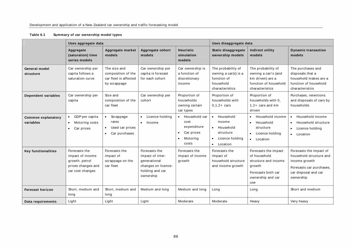
Development and application of a New Zealand car ownership and traffic forecasting model
86
Table 6.1 Summary of car ownership model types
Uses aggregate data Uses disaggregate data
Aggregate
(saturation) time
series models
Aggregate market
models
Aggregate cohort
models
Heuristic
simulation
models
Static disaggregate
ownership models
Indirect utility
models
Dynamic transaction
models
General model
structure
Car ownership per
capita follows a
saturation curve
The size and
composition of the
car fleet is affected
by scrappage
Car ownership per
capita is forecast
for each cohort
Car ownership is
a function of
discretionary
income
The probability of
owning a car(s) is a
function of
household
characteristics
The probability of
owning a car/s (and
km driven) are a
function of household
characteristics
The purchases and
disposals that a
household makes are a
function of household
characteristics
Dependent variables Car ownership per
capita
Size and
composition of the
car fleet
Car ownership per
cohort
Proportion of
households
owning certain
car types
Proportion of
households with
0,1,2+ cars
Proportion of
households with 0,
1,2+ cars and km
driven
Purchases, retentions
and disposals of cars by
households
Common explanatory
variables
GDP per capita
Motoring costs
Car prices
Scrappage
rates
Used car prices
Car purchases
Licence holding
Income
Household car
cost
expenditure
Car prices
Motoring
costs
Household
income
Household
structure
Licence holding
Location
Household income
Household
structure
Licence holding
Location
Household income
Household structure
Licence holding
Location
Key functionalities Forecasts the
impact of income
growth, petrol
prices changes and
car cost changes
Forecasts the
impact of
scrappage on the
car fleet
Forecasts the
impact of inter-
generational
changes on licence-
holding and car
ownership
Forecasts the
impact of income
growth
Forecasts the
impact of
household structure
and income growth
Forecasts the impact
of household
structure and income
growth
Forecasts both car
ownership and car
use
Forecasts the impact of
household structure and
income growth
Forecasts car purchases,
car disposal and car
ownership
Forecast horizon Short, medium and
long
Short, medium and
long
Medium and long Medium and long Long Long Short and medium
Data requirements Light Light Light Moderate Moderate Heavy Very heavy

6 Review of international evidence and forecasting practices
87
Each of these model archetypes is discussed below.
6.2.1 Aggregate time series model
Aggregate time series approaches formed the earliest models and were developed during the 1950s by
Farrell (1954), Cramer (1959) and Tanner (1962). These models fitted an s-curve as a function of time,
with car ownership per capita growing rapidly at moderate levels of car ownership but tapering off as car
ownership approached saturation. The s-curve (see figure 6.1) was used to simulate the product life cycle
of other consumables, with a slow increase in sales during the early years of marketing, a rapid rise as
product acceptance became widespread, and a ‘tailing off’ of new sales as saturation was approached (ie
everyone who wanted one had one). Car ownership was extrapolated into the future, based on an
assumption that car ownership would follow a certain saturation curve.
Figure 6.1 The car ownership s-curve
These aggregate approaches made forecasts using aggregate (ie national) time series data, with the
dependent variable being car ownership per capita and the explanatory variables initially including time
and GDP per capita. Later models such as Tanner (1975) were modified to incorporate other explanatory
variables such as motoring costs. These models implied that a growth in income or motoring costs could
speed up or slow down the approach towards saturation.
Tanner (1977; 1979) introduced a power growth function which approximated a slower approach to the
saturation level. Tanner (1983) then modified the power growth model to accommodate inertia effects.
Other researchers have employed power function curves and Gompertz curves. Dargay and Gately (1999)
estimated Gompertz functions using partial adjustment models, which enabled estimation of short-run
and long-run dynamics.
Aggregate time series models described above have been criticised on a number of grounds. Booz Allen
Hamilton (2000) noted that the initial Tanner model had since been discredited, largely based on the ad
hoc nature of saturation levels (see section 6.2.1.1). Romilly et al (1998) criticised aggregate time series
models that incorporated saturation curves. They argued that hindsight showed that car ownership per
capita did not follow a sigmoid trend (ie s-curve). This criticism was also reflected in the comments of
Whelan, Wardman and Daly (2000).
Time (Year)
Ca
rs/H
ea
d
Saturation level
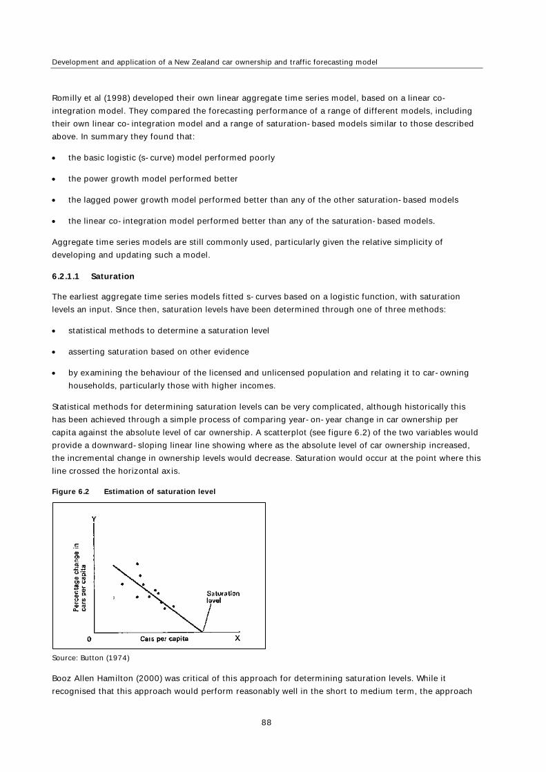
Development and application of a New Zealand car ownership and traffic forecasting model
88
Romilly et al (1998) developed their own linear aggregate time series model, based on a linear co-
integration model. They compared the forecasting performance of a range of different models, including
their own linear co-integration model and a range of saturation-based models similar to those described
above. In summary they found that:
the basic logistic (s-curve) model performed poorly
the power growth model performed better
the lagged power growth model performed better than any of the other saturation-based models
the linear co-integration model performed better than any of the saturation-based models.
Aggregate time series models are still commonly used, particularly given the relative simplicity of
developing and updating such a model.
6.2.1.1 Saturation
The earliest aggregate time series models fitted s-curves based on a logistic function, with saturation
levels an input. Since then, saturation levels have been determined through one of three methods:
statistical methods to determine a saturation level
asserting saturation based on other evidence
by examining the behaviour of the licensed and unlicensed population and relating it to car-owning
households, particularly those with higher incomes.
Statistical methods for determining saturation levels can be very complicated, although historically this
has been achieved through a simple process of comparing year-on-year change in car ownership per
capita against the absolute level of car ownership. A scatterplot (see figure 6.2) of the two variables would
provide a downward-sloping linear line showing where as the absolute level of car ownership increased,
the incremental change in ownership levels would decrease. Saturation would occur at the point where this
line crossed the horizontal axis.
Figure 6.2 Estimation of saturation level
Source: Button (1974)
Booz Allen Hamilton (2000) was critical of this approach for determining saturation levels. While it
recognised that this approach would perform reasonably well in the short to medium term, the approach

6 Review of international evidence and forecasting practices
89
ignored changes in economic influences (eg income, real costs of motoring) on the growth path. It was
also likely that the make-up of the driving population would change over time. For example, recent years
have seen a significant increase in the proportion of female licence holders, due primarily to changes in
social expectations – this change would undoubtedly have increased the level of saturation. It is therefore
feasible to think that saturation levels change through time, thus calling into question statistical
approaches for estimating saturation.
The second approach that has commonly been used is to assert a saturation level using evidence from
other markets. This approach is unsatisfactory due to the factors that are apparent in these markets – in
particular, car ownership levels are lower in Europe because of constraints on parking, better access to
public transport etc. Car ownership in North America is typically higher, due to lower public transport use
in many areas, longer distances travelled (due to urban sprawl), and the lower costs of car ownership. The
propensity to own a car is context specific and difficult to translate to other situations.
The third approach that has been used historically is to examine the characteristics of licensed and
unlicensed drivers. Often the behaviour of the car-owning population with relatively high incomes is
examined and it is then assumed that these people have reached the saturation level of car ownership.
This saturation level is assumed to be applicable to the remaining population as their real income levels
increase over time. The saturation level of per person car ownership will also be influenced by the
following factors:
the proportion of the population who are permitted by law to drive a car
the proportion of the potential car-owning population unable to drive because of physical or mental
disability
the proportion of the potential car-owning population who choose not to own a car.
The above factors can be estimated by various techniques and collected data.
6.2.2 Aggregate market model
Aggregate market models simulate supply and demand in the car market (although the focus is usually on
the used car market). The key driver in these models is a scrappage model – the scrappage model predicts
the rate at which cars are scrapped, based on age and the price of used cars. A used car market model is
used to determine the price of used cars.
The key functionality of these models is that they can be used to predict the composition of the car fleet
because they incorporate the scrapping of used cars. For example, these models are useful for predicting
energy consumption and/or emissions and could be used to predict when a significant amount of energy
inefficient vehicles are going to be retired.
The key output from these models is information about the vehicle fleet. As they use aggregate data they
are unable to relate car purchases to household characteristics such as household structure.
These models require aggregate data on the car market, including the vehicle stock and/or imports,
scrappage rate and used vehicle prices by vehicle type and perhaps by age.

Development and application of a New Zealand car ownership and traffic forecasting model
90
6.2.3 Aggregate cohort model
The cohort approach involves segmenting the population by cohort (ie year of birth) and then making
predictions for each individual cohort. These models forecast car ownership per cohort based on licence
holding and income growth forecasts for each cohort.
Aggregate cohort models are similar to aggregate time series models in that they take aggregate data and
(in effect) extrapolate it into the future.
Aggregate cohort models differ significantly from disaggregate models (eg static disaggregate models)
because they produce data that is person based (rather than household based). Therefore, aggregate
cohort models do not distinguish between first and second cars in the household.
The key functionality of aggregate cohort models is that they take into account inter-generational trends
that can be anticipated. In particular, these models take cohorts into account.
The key outputs from aggregate cohort models are licence holding and the number of cars per person.
Van den Broecke (1987) developed a cohort model that related car ownership in each cohort to licence
holding and income growth in each cohort. A licence-holding model was used to predict licence holding in
each cohort.
6.2.4 Heuristic simulation model
Heuristic simulation models predict car ownership by assuming that households have a budget they spend
on cars. This budget is assumed to be a constant proportion of discretionary income.
The range of possible cars is categorised into car types. These types can be based on fuel type, weight
and/or age of the car.
The households then choose a car type (or a set of car types) that fits within their budget. Households
with high incomes will be able to afford the most expensive car types. Households with low incomes may
not be able to afford any cars.
The key functionality of these models is that they can be used to predict car type choice, in addition to car
ownership. However, the accuracy of the car type choice predictions is questionable because the model
assumes that households choose the most expensive car possible within their budget, and this
assumption is contrary to economic theory.
The key output from these models is car ownership data including data on both the number and types of
cars owned.
6.2.5 Static disaggregate model
The static disaggregate approach makes forecasts using cross-sectional data (ie the car ownership
patterns, income, household structures of a sample of households at a certain point in time).
Cross-sectional data is used to estimate how explanatory variables (such as income and household
structure) influence the probability of households owning a car, or more than one car. The static
disaggregate approach then makes inferences about how car ownership patterns will change in
accordance with expected future changes in income, household structure, etc.

6 Review of international evidence and forecasting practices
91
An early example of the static disaggregate approach was the Netherlands government transport
forecasting model system (LMS), which was developed by Hague Consulting Group (1989). The LMS model
predicts the number of cars owned by a household, given the number of licences in that household.
MVA Consultancy was commissioned by the UK Department of Transport in 1996 to report on an
improved car ownership model. The NRTF car ownership model (DETR 1997a; 1997b) was consequently
developed, which reflected the recommendations of the MVA report.
The 1997 NRTF model was similar to the LMS model. The NRTF model predicted whether a household
owned at least one car, based on licences per adult, household structure, household income and area
type. The model also predicted the probability of the household owning two or more cars (given that it
owned at least one car). The UK Department of Transport acknowledged that an unresolved difficulty of
the car ownership model was the omission of either car purchase prices or fuel prices as explanatory
variables.
Whelan et al (2000) noted that the saturation levels (‘S’) in the 1997 NRTF were an input into the model.
Saturation levels were determined by plotting cars per household against income within each household
category – the levels of car ownership among the highest income groups were then examined.
Whelan et al (2000) noted that saturation levels could be estimated using the aggregate time series
approach described in the preceding section. However, the authors concluded in favour of an approach
that employed disaggregate data. This approach involved estimating the proportion of the population who
were constrained not to own a car (see Whelan et al for more information).
Whelan (2001) audited the 1997 NRTF model and identified a number of possible improvements. The
revised 2001 NRTF model incorporated an additional submodel, which predicted the probability of
households having three or more cars (given that the household had two or more cars). In addition, the
probability of owning two or more cars and the probability of owning three or more cars were both
influenced by the number of company cars the household possessed.
The incorporation of company cars is similar to the approach adopted by the Hague Consulting Group
(2001; 2002) when it developed the Sydney strategic transport model (STM) which explored a range of
options for incorporating company cars:
modelling private and company car ownership independently
modelling private car ownership conditional on company car ownership
modelling company car ownership conditional on private car ownership.
The Hague Consulting Group concluded that the best approach was to model private car ownership
conditional on company car ownership.
6.2.6 Indirect utility model
Indirect utility models replicate household budget decisions. Households select both car ownership and
car use based on household income, fixed car costs and variable car costs. Other explanatory variables
include household size, age, gender and occupation of the head of the household.
Development and application of a New Zealand car ownership and traffic forecasting model
92
The key functionality of these models is that they estimate both car ownership and car use. Furthermore,
these are both estimated within the context of a single model. The key outputs of these models are
predictions of car use and car ownership.
The other functionalities of these models include the fact that they enable estimation of the impact of
household variables such as household income and household structure. In this regard, indirect utility
models are similar to static disaggregate models.
Indirect utility models also have similar data requirements to static disaggregate models. Both models
require disaggregate data on household car ownership and car use (the dependent variables) and
explanatory variables, such as household income, household size and age. The main difference is that
indirect utility models require information on both car ownership and car use.
Indirect utility models are also similar to static disaggregate models in other ways, in that both models
predict car ownership and car use as a function of household explanatory variables. A key difference is
that indirect utility models are constructed based on microeconomic theories about the maximisation of
utility within budget constraints. In contrast, static disaggregate models are not as strongly founded on
microeconomic theories.
6.2.7 Dynamic transaction model
Dynamic transaction models predict future ‘transactions’ (ie purchases and/or disposal of cars). If a
household does not ‘transact’ then car ownership is assumed to be the same as the previous year. The
time between transactions is determined using a duration model. The type of purchase is predicted using
a type-choice model.
The key functionality of these models is that they predict both car ownership and car purchases. In
addition, these models predict the type of purchase without assuming that households can choose a car
instantaneously. The key outputs from these models are broader than most models; the outputs include
both car ownership patterns and car purchases/disposals.
These models require disaggregate household data that relates vehicle purchases to explanatory variables
(income, household structure, location, etc).
These models are similar to static disaggregate models because they use disaggregate data to predict car
ownership. However, dynamic transaction models differ because they predict how car ownership changes
through time (ie they are dynamic).
6.3 Features of key model types
There are three model types which, from our literature review, have been most widely adopted. Their
technical attributes are discussed in this section.
aggregate time series model
static disaggregate model
aggregate market model.
It is also noted that cohort approaches are often incorporated into static disaggregate models.

6 Review of international evidence and forecasting practices
93
6.3.1 Aggregate time series model
6.3.1.1 Inputs
These models employ aggregate time series data on car ownership per capita and varying combinations of
the following explanatory variables:
GDP per capita
motoring costs
car prices
population
vehicle ownership.
Where possible, aggregate time series models should include car prices and GDP per capita, as excluding
GDP can result in misleading forecasts. For example, the Bureau of Transport and Regional Economics
(BTRE) obtained erroneous forecasts because they excluded car costs and GDP from earlier versions of
their CARMOD model. The model failed to anticipate the impacts of recent GDP growth and, in particular, a
recent decrease in real car prices.
Romilly et al (1998) looked at a range of explanatory variables and found that GDP per capita, motoring
costs and bus fares were all significant. Their research is discussed in more detail in section 6.3.1.2.
6.3.1.2 Parameter valuations
Romilly et al (1998) provided the most econometrically robust estimates of parameter valuations for an
aggregate time series model:
Table 6.2 Cointegration and error-correction model estimates, Romilly et al (1998)
Dependent variable: car ownership per capita
Short run Long run
Time trend 0.09 -0.04
Real personal disposable income per capita 0.34 1.14
Real motoring cost index -0.29 -2.19
Real bus fare 0.09 1.70
The estimates produced by Romilly et al showed the following:
a 1.0% increase in income caused car ownership per capita to increase by 0.3% in the short-run (ie
within a year) and 1.1% in the long-run
a 1.0% increase in motoring costs caused car ownership per capita to decrease by 0.3% in the short-
run and 2.2% in the long-run
a 1.0% increase in real bus fares caused car ownership per capita to increase by 0.1% in the short-run
and 1.7% in the long-run
the estimates of long-run impacts were all larger than the estimates of short-run impacts – this
finding is consistent with economic theory.

Development and application of a New Zealand car ownership and traffic forecasting model
94
Romilly et al also estimated the impacts of unemployment rate, size of road network, real interest rate and age
structure. But these variables were not statistically significant so they were excluded from the final model.
6.3.1.3 Outputs
The main output from an aggregate time series model is an estimate of car ownership per capita. An
aggregate time series model can also produce an estimate of ‘saturation’ (ie long-run) car ownership per
capita, but the accuracy of this is yet to be proved.
6.3.1.4 Model function
As discussed earlier, aggregate time series models generally fit an s-curve to time series data. This s-
curve approach was pioneered by Tanner (1958; 1962). The Tanner approach assumed that car ownership
could be predicted by the following equation:
(Equation 6.1)
where:
Ct = cars per capita at time t
t = time
S = saturation
a, b = constants
The equation above assumes that the growth rate diminishes as cars per capita grows. By fitting data to
this curve, the country’s position along that saturation curve can be estimated.
The approach above was modified by Tanner (1974) to accommodate causal variables of income and
motoring costs. The model implied that a growth in income or decrease in motoring costs could ‘speed
up’ the approach towards saturation. Tanner (1977; 1979) then revised this approach to incorporate a
power function, so that saturation was approached more gradually:
(Equation 6.2)
where:
Ct = cars per capita
t = time
i = per capita income
P = real motoring costs
a, b, c, d, n = constants
The Tanner approach has also been modified using a Gompertz curve. The general model form below was
adopted by Van Der en Buningh (1978) and Dargay and Gately (1999):
(Equation 6.3)
where:
Ct = cars per capita
t = time
S = Saturation
i = per capita income or other independent variable
a, b = constants
(see Ogut 2004).
1t bt
SC
ae
1 ( ln( ) ln( ))t n
SC
a bt c i d P
biaetC Se

6 Review of international evidence and forecasting practices
95
However, all of these s-curve approaches have the same basic shape with varying degrees of steepness at
different points along the curve.
The s-curve approaches described above have the following functional limitations:
In these models, the forecast level of saturation is assumed to be constant, regardless of changes in
income, attitudes, car prices or fuel cost. Such variables may affect the speed at which the economy
approaches saturation, but they do not affect the actual saturation level.
These models do not provide information about the types of cars or the number of cars owned by
households
6.3.1.5 National models
The BTRE has developed a car ownership/use model for Australia, using aggregate time series techniques.
The original model assumed that vehicle ownership followed a simple logistic function over time. This
model failed to anticipate the recent surge in car ownership (which appears to have been driven by GDP
growth and decreases in real vehicle prices). However, this model has been modified due to short-
comings in forecasting performance.
The modified model is unusual because it directly estimates VKT per capita without calculating cars per
capita. VKT per capita is estimated using a logistic saturation curve. Interestingly, the trend in VKT per
capita is consistent with a saturation curve. This model then derives VKT per car and cars per capita as an
output of the VKT per capita forecasts described above. VKT per car is estimated as a function of GDP,
trend in household ownership of cars and projected changes in the proportion of the population of
working age.
6.3.2 Static disaggregate model
6.3.2.1 Inputs
Static disaggregate models estimate the impacts of household-based explanatory variables (household
structure, household income etc) on household car-ownership patterns. Therefore, static disaggregate
models require data for a sample of households – the data should show the number of cars the household
owns and any explanatory variables of interest. The key inputs into static disaggregate models are
household structure, household income and the licence-holding patterns within the household.
Unfortunately, static disaggregate models generally only use cross-sectional data – data from a sample of
households at a point in time (or, at best, data from a sample of households at a few points in time).
Therefore, incorporating variables that are constant across households (eg petrol prices, car prices) into
static disaggregate models is problematic.
Static disaggregate models require other models as inputs. In particular, a model is required to forecast
the number of households in each household structure category. In addition, a model is required to
forecast income growth for each of the static disaggregate models sub-groups (eg area type, household
structure type)
Static disaggregate models can be used to produce forecasts at sub-regional levels. For example, the UK
NRTF model enables estimates of future car ownership to differ by area type. There are five area types in
the NRTF model:

Development and application of a New Zealand car ownership and traffic forecasting model
96
Greater London
metropolitan districts
districts with density 10+ persons per hectare
districts with density 2.0 to 10.0 persons per hectare
districts with density 0.0 to 2.0 persons per hectare.
The NRTF model analysed some 130,000 households and extracted datasets on:
gross household Income
number of adults
number of children
total number employed
number of retired adults
area type (as above)
number of cars and vans.
6.3.2.2 Outputs
Static disaggregate models produce outputs by breaking the population down into subgroups (eg region
and household type) and then estimating the probability of a household in that subgroup owning a car.
These probabilities are then combined with the number of people in that sub-group, producing the total
number of households in that sub-group with at least one car. A similar process is used for estimating the
number of households with two or more cars. Therefore, the static disaggregate model can be used to
estimate of the number of households with zero, one, two or more cars. This output is a key advantage of
static disaggregate models because it seems highly plausible that the number of kilometres driven by a
household is influenced by the number of cars that the household owns. Static disaggregate models are
often also used to predict company car ownership.
6.3.2.3 Model function
Probability models are used to predict whether a household owns zero, one, two or more vehicles based
on household variables.
The NRTF model has the following structure:
There are three binary choice models that examine the household decision to own one or more vehicles
(P1+), two or more vehicles conditional on the ownership of one of more vehicles (P2+1+), and three or
more vehicles conditional on the ownership of two or more vehicles (P3+2+).
The mathematical equations are as follows:
(Equation 6.4)
1
11
1
ahU
SP
e

6 Review of international evidence and forecasting practices
97
3 2
33
1
ah
U
SP
e
Where:
S = saturation level by area (a) and household type (h)
U = the utility of ownership
The utility of ownership equations include the following variables:
number of driving licences per adult for all of Great Britain
household income
household type
area
number of adults employed
purchase cost index
vehicle use cost index
number of company cars in the household.
The Sydney STM consists of the following sub-models:
a model to predict licence holding by household
a model to predict car ownership, conditional on licence holding
a model to predict the frequency of trips to work, by employed individuals.
Model for licence holding
In Sydney, between 1971 and 1998, licence holding increased from 62% to 81%. It was estimated that
around 80% of this increase could be attributed to the ‘catching up’ of women’s licence holding relative to
men’s licence holding. This occurred due to the replacement of older generations of women who had low
licence holding by younger women, who had licence holding similar to men.
The report notes that many car ownership models include a ‘trend’ variable representing increasing car
ownership that cannot be explained by income. This ‘trend’ can be attributed, at least in part, to a growth
in licence holding. Therefore, it is important that projections into the future take into account the impact
of licence holding.
The Sydney STM predicts the likelihood of households being in one the following four states:
neither member of household has a licence
head of household has a licence; partner does not have a licence
head of household does not have a licence; partner does have a licence
2 1
22
1
ahU
SP
e

Development and application of a New Zealand car ownership and traffic forecasting model
98
both head of household and partner have a licence.
Households are more likely to have licences as income increases, the number of children increases and
with the presence of employment.
Households are less likely to have licences if the head of the household is female, the head of the
household is under 25 or over 70 or if the household is large.
Model for car ownership
The Sydney STM company car ownership model predicts the probability of households having the
following:
no company cars
1 company car
2 company cars.
The predictions of the company car ownership model are influenced by (the log of) household income, the
number of licences in the household, the ages of the household members and the presence of a female
head of household.
Then, the Sydney STM total car ownership model predicts the probability of households having the
following:
0 cars
1 cars
2 cars
3 or more cars.
The predictions of the total car ownership model are influenced by (the log of) household income, the
number of licences in the household, the ages of the household members, the presence of company cars
and the employment status (part-time, full-time) of the members of the household.
6.3.2.4 National models
The UK Department for Transport (DfT) has had a car ownership model for many years. The original NRTF
model was based on an aggregate time series model and used s-shaped growth curves incorporating
income, motoring costs and time as explanatory variables.
In the late 1990s the DfT moved to a disaggregate model. Since then the model has undergone updates to
extend the car ownership choice levels (to three or more cars), include company cars, assess the impacts
of employment levels and to include purchase and use costs.
6.3.3 Aggregate market model
6.3.3.1 Inputs
Aggregate market models simulate supply and demand in the car market. Their key driver is a scrappage
model which predicts the rate at which cars are scrapped based on age and other factors. These models
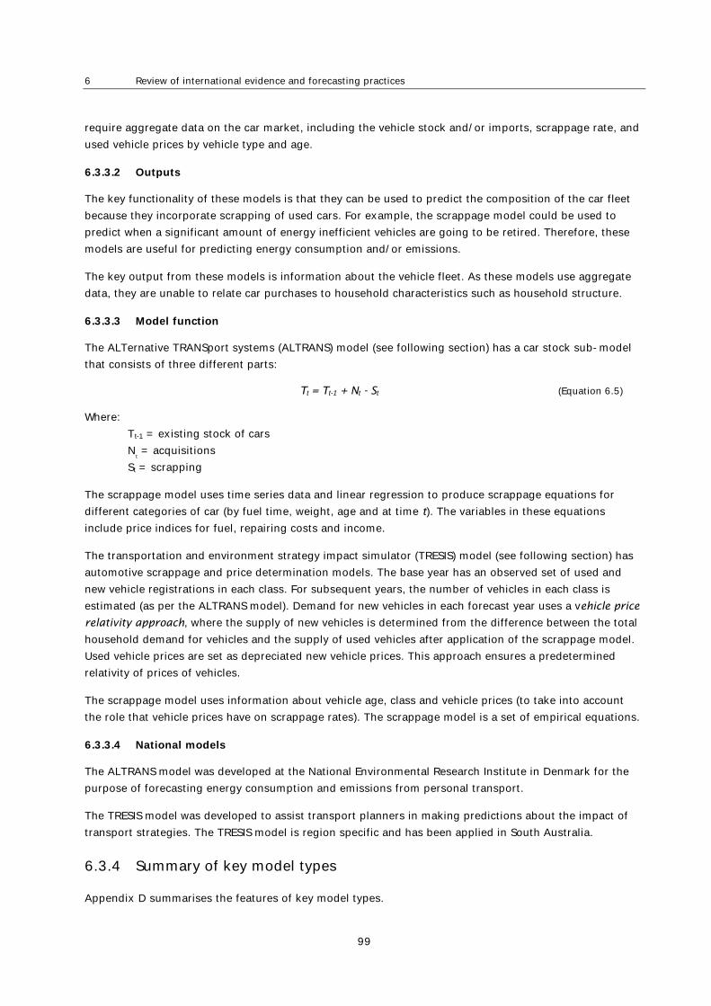
6 Review of international evidence and forecasting practices
99
require aggregate data on the car market, including the vehicle stock and/or imports, scrappage rate, and
used vehicle prices by vehicle type and age.
6.3.3.2 Outputs
The key functionality of these models is that they can be used to predict the composition of the car fleet
because they incorporate scrapping of used cars. For example, the scrappage model could be used to
predict when a significant amount of energy inefficient vehicles are going to be retired. Therefore, these
models are useful for predicting energy consumption and/or emissions.
The key output from these models is information about the vehicle fleet. As these models use aggregate
data, they are unable to relate car purchases to household characteristics such as household structure.
6.3.3.3 Model function
The ALTernative TRANSport systems (ALTRANS) model (see following section) has a car stock sub-model
that consists of three different parts:
Tt = Tt-1 + Nt - St (Equation 6.5)
Where:
Tt-1 = existing stock of cars
Nt = acquisitions
St = scrapping
The scrappage model uses time series data and linear regression to produce scrappage equations for
different categories of car (by fuel time, weight, age and at time t). The variables in these equations
include price indices for fuel, repairing costs and income.
The transportation and environment strategy impact simulator (TRESIS) model (see following section) has
automotive scrappage and price determination models. The base year has an observed set of used and
new vehicle registrations in each class. For subsequent years, the number of vehicles in each class is
estimated (as per the ALTRANS model). Demand for new vehicles in each forecast year uses a vehicle price
relativity approach, where the supply of new vehicles is determined from the difference between the total
household demand for vehicles and the supply of used vehicles after application of the scrappage model.
Used vehicle prices are set as depreciated new vehicle prices. This approach ensures a predetermined
relativity of prices of vehicles.
The scrappage model uses information about vehicle age, class and vehicle prices (to take into account
the role that vehicle prices have on scrappage rates). The scrappage model is a set of empirical equations.
6.3.3.4 National models
The ALTRANS model was developed at the National Environmental Research Institute in Denmark for the
purpose of forecasting energy consumption and emissions from personal transport.
The TRESIS model was developed to assist transport planners in making predictions about the impact of
transport strategies. The TRESIS model is region specific and has been applied in South Australia.
6.3.4 Summary of key model types
Appendix D summarises the features of key model types.

Development and application of a New Zealand car ownership and traffic forecasting model
100
6.4 Examples of international models
Table 6.3 summarises the following international car ownership models, based on published literature.
These models were selected for review as information was readily available. These models have been
adopted in various countries and applied at a national level, as discussed previously in this section:
NRTF model – United Kingdom
ALTRANS model – Denmark
CARMOD model – Australia
TRESIS model – Australia
STM model – Australia
FACTS models – Netherlands.
Appendix E provides more detail on each of these models.

6 Review of international evidence and forecasting practices
101
Table 6.3 National models
Model CARMOD STM TRESIS NRFT FACTS ALTRANS
Country Australia Australia Australia UK UK The Netherlands Denmark
Developer Bureau of
Transport and
Regional
Economics (BTRE)
Hague Consulting
Group and the
Institute of
Transport Studies
See Hensher and Ton
(2002)
Department of the
Environment, Transport
and the Regions
Department of
the Environment,
Transport and
the Regions
The Transport Research
Centre (AVV) of the
Dutch Ministry of
Transport
See Kveiborb
(1999)
Year 2002 2001 2002 1997 1997 2002 1999
Objective To forecast
greenhouse gas
emissions
To forecast travel
patterns (including
mode-choice and
trip patterns) in the
Greater Sydney
Metropolitan
Region
To forecast the impact
of a wide range of
policies (eg congestion
pricing, new
infrastructure, land-use
change, and PT service
changes) on variables of
interest, including
kilometres driven,
energy use, emissions,
and mode share.
To forecast national
traffic levels
To forecast
national traffic
levels
To forecast emissions
from the transport fleet
To forecast
energy
consumption
and emissions
from personal
transport
Relevance to
VKT and/or
car
ownership
End-model
estimates fuel use.
Sub-model
estimates VKT per
capita but this is
only used to derive
cars per capita
Car ownership
model and work
trip model
Car ownership model Car ownership model Car use model Car ownership model
and car use model
Car ownership
model
General
category of
model
(RAND)
Aggregate time
series –
‘saturation’ curve
for VKT per capita
Static disaggregate
ownership model
Aggregate car market
model of total demand,
scrappage and new
purchases.
Static disaggregate
ownership model
Static
disaggregate use
model, combined
with an
aggregate time
series model.
Heuristic simulation
model, in which
expenditure (on vehicle
and kilometres driven)
is a heuristic function
of household budget.
Aggregate car
market model
of stocks,
acquisitions
and scrappage.

Development and application of a New Zealand car ownership and traffic forecasting model
102
Model CARMOD STM TRESIS NRFT FACTS ALTRANS
General
structure
Fuel use is
assumed to be a
function of cars
per capita,
population, VKT
per car and fuel
efficiency.
Cars per capita is
derived from
estimates for VKT
per capita and VKT
per car.
VKT per capita is
the ‘driver’ of the
forecasts and this
is related to GDP
per capita using a
logistic ‘saturation’
function.
A licence-holding
model predicts the
number of licences
in each household,
using explanatory
variables such as
age dummies and
employment status
of household
members..
A car ownership
model predicts the
number of cars
owned by
households – This
stage consists first
of a company car
ownership model
and second, a total
car ownership
model, conditional
on company car
ownership.
A travel frequency
model is also used
to predict the
number of work
‘tours’ made by
each employed
individual.
A scappage model
determines scrappage
based on the age of
used cars and used car
prices. Used car prices
are influenced by the
exogenous price of new
cars. New purchases are
determined as the
difference between total
demand for cars and
the supply of used cars
(after scrappage).
A household sub-model
is used to estimate the
number of households,
by eight household
types.
Income is assumed to
grow at 2.5% from 1996
to 2001 and 2.25% from
2001 to 2031.
The probability of
owning at least one car
was estimated as a
function of forecast
income (modified by
region & household
type) and forecast
licences per adult.
The probability of
owning two cars (if the
household owns at least
one car) was estimated
as a function of forecast
income (modified by
region & household
type) and forecast
licences per adult.
Licences per adult was
forecast using cohort
data.
The probabilities are
combined with the
forecast number of
household types, to
produce forecasts for
car ownership.
A cross-sectional
model is used to
calculate car use
elasticities,
broken down by
household type
and car
ownership
numbers – These
are then used to
produce initial
car use forecasts.
A fuel cost
elasticity is
estimated and
this is used to
modify car use
forecasts.
The car use
forecasts are
modified in the
end by a
company car
adjustment.
A simulation model
creates a number of
households.
Households are
allocated a certain
number of kilometres
driven.
Households then select
the best car that they
can, given the
proportion of their
budget allowed for
expenditure on cars
and kilometres driven.
The household may not
be able to afford a car;
alternatively, the
household may be able
to afford multiple cars.
A ‘scrappage
model’ is
developed to
predict car
scrappage (by
fuel type,
weight and
age) and a
‘behavioural
model’ predicts
the car stock.
The remainder
is assumed to
be vehicle
acquisitions.

6 Review of international evidence and forecasting practices
103
Model CARMOD STM TRESIS NRFT FACTS ALTRANS
National
regional
applications
No regional
components
The model is
specifically
designed for
application to the
Sydney region.
The model is integrated
and is modified to take
into account the details
of each region
No regional forecasts,
other than for area-
types (ie Greater
London, Metropolitan
districts and three other
categories with
differing levels of
population density).
No regional
forecasts
No regional forecasts
mentioned
No regional
forecasts
mentioned
Forecast
time period
Forecasts to 2020 Forecast period not
stated
Forecasts for 1998,
2003, 2008 and 2013
Forecasts to 2031 Forecasts to
2031
Forecasts period not
stated
Forecasts are
not discussed
in detail
Variables
involved in
model
(and
sensitivity)
GDP per capita
Fuel prices
Car prices
Proportion of
population of
working age
‘Trend in
Household
ownership of
vehicles’
Employment
status
Female head of
household
Number of
children
Income of head
of household
Income of
partner
Parking cost
Number of
licences in
household
Price of new cars
Age of existing fleet
Commuter mode
choice
(note –variables not
explicitly identified)
Numbers of people
in each household
type
GDP per capita (with
income effect
modified by region
and household type)
Licence holding
Numbers of
people in
each
household
type and
their location
Forecasts of
car
ownership by
household
type
GDP per
capita (by
household
type)
Fuel cost
(including
fuel prices
and fuel
efficiency)
Income
Share of income
spent on cars
Vehicle prices
(perhaps)
Income
Fuel prices
Repair costs
Acquisition
costs
Coverage
(cars, all)
All cars – no
distinction
All cars – no
distinction
Cars distinguished by
age, size and fuel-type
All cars – no distinction All cars – no
distinction
Cars distinguished by
18 car types (including
fuel-type) and age
(>5,<5)
Cars
distinguished
by fuel-type,
age and weight

Development and application of a New Zealand car ownership and traffic forecasting model
104
Model CARMOD STM TRESIS NRFT FACTS ALTRANS
Critique and
commentary
The cars per capita
variable does not
appear to be an
explanatory
variable; rather, it
appears to be the
level of car
ownership
deduced given the
forecasts for VKT
per capita and VKT
per car
The model is
statistically robust
because it uses
cross-sectional
data.
The paper
describes cohort
analysis of licensing
patterns but does
not use the cohorts
to predict future
licensing
The licencing and
car ownership
models use dummy
variables for age,
rather than
continuous
variables.
The paper/s do not
discuss the details of
the model.
The model does not
appear to incorporate
common explanatory
variables for car
ownership, such as
income, but this may be
because these have not
been stated.
The scrappage model,
which bases scrappage
on age and used car
prices, seems to be a
useful model for
development of car
ownership model with
details about the fleet.
The model entails an
assumption that used car
prices are related to new
car prices, which may or
may not be correct.
The model is
statistically robust
because it uses cross-
sectional data.
The model is incoherent
because licence holding
feeds through both as a
constraint – via
‘saturation’ levels – and
as an explanatory
variable via licences per
adult.
The model is
statistically
robust because it
uses cross-
sectional data,
but it has the
added benefit of
using time series
data to produce
fuel cost
elasticities
The model is counter-
intuitive because it
assumes that people
maximise expenditure
on cars.
In addition, the model
only has a few
explanatory variables
(income, share of
income spent on cars)
and does not seem to
account for other
variables, such as fuel
prices.
The impact of
the explanatory
variables is not
discussed in
detail.
The model is
very effective at
describing the
composition of
the fleet, and
hence
emissions, but
is less
appropriate for
predicting
traffic
Key
references
There are no key
references
There are no key
references
The paper refers to
Hensher and Greene
(2000) who use logit
models and RP/SP data
to develop a model of
car choice. Variables
that affected car choices
included car price and
running costs, engine
size, acceleration and
boot size.
There are no key
references
There are no key
references
There are no key
references
The paper
refers to an
‘acquisitions
model’
developed by
Cowi (1998)

7 Development of a recommended New Zealand modelling framework
105
7 Development of a recommended New Zealand modelling framework
7.1 Introduction
This section considers the development of a New Zealand modelling framework and methodology for car
ownership and traffic forecasting. This has been based on the previous research that:
examined New Zealand literature and current car ownership models
reviewed New Zealand car ownership and use trends and data
examined international car ownership models
considered results from the ‘needs survey’ that was undertaken.
The methodology could be a new modelling suite, or an enhancement to an existing platform currently
being used.
7.2 Potential model types
Section 5 reviewed the New Zealand models for car ownership while section 6 reviewed the types of
models currently used internationally for car ownership and traffic forecasting.
There are three main types of car ownership models that are commonly used internationally as national
car ownership car models. These are:
aggregate time series models
static disaggregate models
aggregate car market model
The following section compares the three model types with the functional requirements detailed in section
4 that came out of the needs survey.
7.2.1 Aggregate time series models
New Zealand examples of the aggregate time series models are used in the MoT’s VFEM and the Tauranga
transport model. An aggregate time series model was also developed in this research (section 3).
International examples include the Australian Bureau of Transport and Regional Economics (BTRE)
CARMOD model.
Table 7.1 below compares the desired functionality with the general aggregate time series model.

Development and application of a New Zealand car ownership and traffic forecasting model
106
Table 7.1 Aggregate time series model
Desired functionality Meets
requirements
Comment
Include segments of vehicles (eg private,
company, LCVs) XX
Not included in models
Ability to apply at national, regional and local
contexts
The models provide a national forecast that can
be applied to regional and local contexts
Focus on 25-year horizon Models perform better in short-medium term
Include link between household structure and
demographics XX
Models do not specifically include link to
household structure and demographics
Segments vehicles by fuel type/efficiency
-
Models do not include, but as with the MoT VFEM
can be supplemented with an additional model
Sensitive to changes in income
Models can include GDP/capita as an explanatory
variable.
Sensitive to changes in fixed/variable vehicle
costs
Models can include car price index as an
explanatory variable
Sensitive to the level of PT/TDM/land-use supply XX
Not included in models
Outputs should include vehicle numbers, traffic
forecasting and fuel consumption measures - Separate models are required for traffic
forecasting and fuel consumption, as with the
VFEM
Key: meets requirements, somewhat meets requirements, - potential to meet requirements, X unlikely to meet
requirements, XX does not meet requirements
It is clear that the aggregate model type, an example of which is reported in section 5 and is also used in a
number of New Zealand models, is not able to provide all of the desired features specified in the needs
survey. However, it is important to note that the data requirements for such models are relatively light and
these types of models are currently used in New Zealand.
7.2.2 Static disaggregate models
A form of a static disaggregate car ownership model is used in the Auckland Regional Transport (ART2)
model. An international example is the UK DfT (NRTF) model.
Table 7. compares the desired functionality with the general static disaggregate model.

7 Development of a recommended New Zealand modelling framework
107
Table 7.2 Static disaggregate model
Desired functionality Meets
requirements
Comment
Include segments of vehicles (eg private, company,
LCVs) Models can include
Ability to apply to national, regional and local
contexts Models can include area types
Focus on 25-year horizon Models perform well over the medium-long
term
Include link between household structure and
demographics Models are based on detailed household
structure information
Segment vehicles by fuel type/efficiency X Vehicles are not segmented by type
Sensitive to changes in income Income is an explanatory variable
Sensitive to changes in fixed/variable vehicle costs Car purchase prices and use costs are
explanatory variables
Sensitive to the level of PT/TDM/land-use supply Area type can be used as a proxy for PT and
accessibility
Outputs should include vehicle numbers, traffic
forecasting and fuel consumption measures NRTF model provides these outputs
Key: meets requirements, somewhat meets requirements, - potential to meet requirements, X unlikely to meet
requirements, XX does not meet requirements
It is clear that static disaggregate model types are able to provide most of the features that are desired.
However, it is important to note that the data requirements for these models are relatively significant.
7.2.3 Aggregate car market models
International examples of an aggregate car market model include the Denmark ALTRANS model and the
Australian TRESIS model.
Table 7.3 below compares the desired functionality of a New Zealand car ownership model with the
general aggregate car market model.
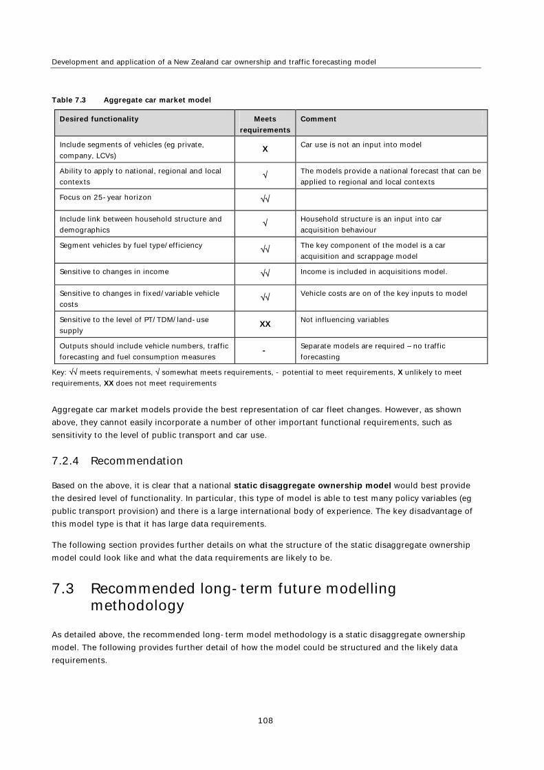
Development and application of a New Zealand car ownership and traffic forecasting model
108
Table 7.3 Aggregate car market model
Desired functionality Meets
requirements
Comment
Include segments of vehicles (eg private,
company, LCVs) X Car use is not an input into model
Ability to apply to national, regional and local
contexts The models provide a national forecast that can be
applied to regional and local contexts
Focus on 25-year horizon
Include link between household structure and
demographics Household structure is an input into car
acquisition behaviour
Segment vehicles by fuel type/efficiency The key component of the model is a car
acquisition and scrappage model
Sensitive to changes in income Income is included in acquisitions model.
Sensitive to changes in fixed/variable vehicle
costs Vehicle costs are on of the key inputs to model
Sensitive to the level of PT/TDM/land-use
supply XX Not influencing variables
Outputs should include vehicle numbers, traffic
forecasting and fuel consumption measures - Separate models are required – no traffic
forecasting
Key: meets requirements, somewhat meets requirements, - potential to meet requirements, X unlikely to meet
requirements, XX does not meet requirements
Aggregate car market models provide the best representation of car fleet changes. However, as shown
above, they cannot easily incorporate a number of other important functional requirements, such as
sensitivity to the level of public transport and car use.
7.2.4 Recommendation
Based on the above, it is clear that a national static disaggregate ownership model would best provide
the desired level of functionality. In particular, this type of model is able to test many policy variables (eg
public transport provision) and there is a large international body of experience. The key disadvantage of
this model type is that it has large data requirements.
The following section provides further details on what the structure of the static disaggregate ownership
model could look like and what the data requirements are likely to be.
7.3 Recommended long-term future modelling methodology
As detailed above, the recommended long-term model methodology is a static disaggregate ownership
model. The following provides further detail of how the model could be structured and the likely data
requirements.

7 Development of a recommended New Zealand modelling framework
109
7.3.1 Overview and structure
The UK NRTF model has had considerable development over the last decade and has accessible
documentation. The proposed structure and data requirements are based on the latest version of this
model.
7.3.1.1 Car ownership model
Figure 7.1 shows the overall proposed structure of the car ownership model. Each of the key components
of the model is described in further detail below. This structure is based on the latest updates to the UK
car ownership model (DETR 2007 and Whelan 2001).
Figure 7.1 Car ownership model framework
Household sub-model
Future population forecasts are usually in the form age–sex distribution and total people. This data then
needs to be converted into future household characteristics. The household sub-model uses the existing
household survey to produce a sample of households that is internally consistent (the household survey is
unlikely to be directly representative of the population) while also achieving consistency with aggregate
statistics. The technique of ‘prototypical sample enumeration’ can be used, which utilises the existing
sample in the base year while meeting the targets in the forecast years.
Household Sub-Model:Estimates the number of households by each household type (eg one adult, not retired) and by each area type
Household Sub-Model:Estimates the number of households by each household type (eg one adult, not retired) and by each area type
Input Assumptions:Information and forecasts of:•Income by household type•Age specific licence holding•Car ownership saturation by household type•Car purchase costs•Vehicle use costs•Employment•Company car availability
Input Assumptions:Information and forecasts of:•Income by household type•Age specific licence holding•Car ownership saturation by household type•Car purchase costs•Vehicle use costs•Employment•Company car availability
Estimates of Probabilities of Car Ownership:Calibration of the sub models:•Binary Logit Models•Utility of Ownership
Estimates of Probabilities of Car Ownership:Calibration of the sub models:•Binary Logit Models•Utility of Ownership
Car Ownership Forecasts:By year, area type, household and car type
Car Ownership Forecasts:By year, area type, household and car type
Binary Logit Models:•Separate models for probability of household owning 1, 2 & 3+ cars•Saturation level varying by area and household type•Influenced by Utility of Ownership
Binary Logit Models:•Separate models for probability of household owning 1, 2 & 3+ cars•Saturation level varying by area and household type•Influenced by Utility of Ownership )exp(1 1
11
U
SP ah
Utility of Ownership Models:•Calibrated to: drivers licences per adult, household income, household type, area type, adult employed, purchase costs, vehicle use costs and number of company cars•Separate models for probability of household owning 1, 2 & 3+ cars
Utility of Ownership Models:•Calibrated to: drivers licences per adult, household income, household type, area type, adult employed, purchase costs, vehicle use costs and number of company cars•Separate models for probability of household owning 1, 2 & 3+ cars
Key
Inputs
Key Models
Input Models
Output
Aggregate Model:Cross-check of forecasts
Aggregate Model:Cross-check of forecasts

Development and application of a New Zealand car ownership and traffic forecasting model
110
Binary logit models
The binary models assess household decisions to own zero, one, two or three vehicles. The form of the
equations is as follows:
(Equation 7.1)
Where:
P+ is the probability of a household owning one or more vehicles
P2+I1+ is the probability of a household owning two or more vehicles, conditional on the ownership
of one or more vehicles
S is the saturation level by area (a), household type (h) and U is the utility of ownership (see below).
Utility of ownership models
The utility models are related to the socio-economic characteristics of the household, geographical-
location, car purchase and use costs, and average licence holding. The models are in the form of:
(Equation 7.2)
Where:
LPA is the number of driver licences per adult in NZ
Y is the household income
Dh is a vector of household type dummy variables
Da is a vector of area type dummy variables
E is the number of adults employed
O is an index of purchase costs
R is an index of vehicle use costs
CC1 is a dummy variable if there is one company car in the household
CC2 is a dummy variable if there are two company cars in the household

7 Development of a recommended New Zealand modelling framework
111
ASC is a vector of alternative specific constants
b,c,d,e,f and g are parameter vectors (estimated)
Aggregate model
An aggregate model, as developed in section 3 of this report, could provide a cross-check on the sum of
the disaggregate model forecast.
Process of applying model
The models, detailed above, can be used to develop ownership forecasts for particular zones (eg census
zones). A six-stage process is used to apply the models:
1 Base sample definition
The base sample of the population households is defined from survey information.
2 Target area definition
The second stage is to define the geographical ‘target’ areas for which the forecasts are required (eg
census zone areas or larger areas).
3 Forecasting period definition
Forecasts are required at five-yearly internals for the forecast period.
4 Target variable definition
In this stage the aggregate socio-demographic characteristics of each target area in each time interval are
described in terms of the target variables (see below). A sampling method is used to generate artificial
disaggregate samples that when aggregated, match the totals of the target variables and also maintain the
detailed relationships in the base-year data.
Target variables could include:
the number of people who live in the zone
the number of children aged between 0 and 15 in the zone
the number of males in the zone, aged between 16–64 in fulltime employment
the number of males in the zone, aged between 16–64 in part-time employment
the number of males in the zone, aged between 16–64 who are students
the number of males in the zone, aged between 16–64 who are neither students nor employed
the number of males in the zone who are 65 or more years old
as above for females
the total number of people in the zone in employment
the number of single person households in the zone
the number of households in the zone with more than one person

Development and application of a New Zealand car ownership and traffic forecasting model
112
the number of company cars in the zone.
While household income is not included in the above target variables, the variation in income levels across
zones is achieved by factoring income levels in each zone.
5 Household category
Households are grouped into pre-defined categories that cover the key dimensions of the sample.
6 Adjusting constraints
To ensure that the model is able to replicate the base ownership probability for each zone, the model
constants (ASCs) are adjusted so that the forecast matches the actual ownership levels from the base year
census information.
The outputs form the car ownership forecasts (by year, area type, household and car type) can then be
applied at a regional/local level. This would be done by applying the forecasts to the regional/local
estimate of area types and household types.
7.3.1.2 Traffic forecasting (car use) model
Figure 7.2 below shows the overall proposed structure of the traffic forecasting model. Each of the key
components of the model are described in further detail below. This structure has been based on the UK
car use model (DETR 1997a; 1997b).
Figure 7.2 Traffic forecasting model
Cross-sectional model
In order to be compatible with the car ownership model, traffic forecasting should also use the same
household types. In the cross-sectional model the ‘first’ car is defined as the car with the highest use (ie
kilometres travelled) and the ‘second’ car includes the use of any additional cars.
Input Assumptions:Forecasts of:•Changes in household types and location•Car ownership by household type•Income by household type
Input Assumptions:Forecasts of:•Changes in household types and location•Car ownership by household type•Income by household type
Cross-Sectional Model:Estimates elasticities of car use for each household type and ownership type
Cross-Sectional Model:Estimates elasticities of car use for each household type and ownership type
Time Series Model:Estimates of aggregate elasticity of car use with respect to changes in fuel costs
Time Series Model:Estimates of aggregate elasticity of car use with respect to changes in fuel costs
Car Use Forecasts:Forecasts of annual car use per car
Car Use Forecasts:Forecasts of annual car use per car
Company Car Adjustment:Adjustment to take into account company car use
Company Car Adjustment:Adjustment to take into account company car use
Input Assumptions:Forecasts of:•Fuel prices•Fuel efficiency•National GDP
Input Assumptions:Forecasts of:•Fuel prices•Fuel efficiency•National GDP
Key
Inputs
Key Models
Output

7 Development of a recommended New Zealand modelling framework
113
The model could be based on a national travel survey with the following explanatory variables:
real gross annual household income
number of employed people per household
proximity of bus services
proximity to rail services
a variable to indicate whether the head of the household is disabled
a variable indicating the location of the household (eg if there are five generic locations then there will
be five variable values)
a variable to indicate whether the head of the household is a full-time student
a variable indicated whether the car modelled is a company car.
The form of the cross-sectional model is as follows:
(Equation 7.3)
All variables, except income, are discrete dummy variables (either a value of 0 or 1). For example, if there
is one or more persons employed in the household the employment variable is 1, otherwise it is 0. The log
form of car use and income means that the estimated income elasticities are constant across all income
levels within each household type.
Using regression analysis, the elasticities of car use by household type and car type (eg first or second car)
are determined.
Time series model
The above cross-sectional model does not incorporate time dependent determinants of traffic forecasting.
The key influencing variable of car use is fuel cost. The elasticity of traffic forecasting with respect to fuel
costs over time is influenced by:
fuel costs themselves (including tax changes over time)
personal or household income
fuel efficiency of vehicles.
Using regression analysis, elasticities for car use with respect to fuel can be derived. In order to provide a
time series model, assumptions will need to be made on how the above variables will change with time.
Company car adjustment
Company car use is generally higher than private-ownership car use as the fuel costs and other running
costs are paid for (or contributed to) by a company. An exaggeration of traffic forecasting could occur if it
is assumed that as a household moves from a one-car to a multi-car household they adopt the same
company car rate as existing multi-car households. To avoid potential overestimation of traffic
log( ), , , ,
, , ,log ( )
income employment bus services rail services
disabilities houshold area type student company car statuscar use function

Development and application of a New Zealand car ownership and traffic forecasting model
114
forecasting, in the future it can be assumed that the overall proportion of company cars in each household
type remains unchanged and an adjustment factor calculated.
7.3.2 Data requirements
The data requirements have been based on the above proposed structure (UK models). The data
requirements have then been compared with the currently available New Zealand data to identify gaps
where additional data would need to be collected.
7.3.2.1 Car ownership model
The UK car ownership models are based on data from:
the Expenditure and Food Survey (formally Family Expenditure Survey) and the National Travel Survey
to form household car ownership data
constructed indices for car ownership costs, car running costs, general prices (CPI) and historical
trends on the average number of driving licences per adult.
Household car ownership data
Household datasets (for multiple years, last 20–30 years) is required including:
gross household income
number of adults
number of children
total number employed
number of retired adults
area type
number of cars and vans (separated by company and private).
The UK dataset had 7000–15,000 observations in each dataset. Datasets were collected every five years
from 1971 to 1996, and then yearly from 1997.
The New Zealand five-yearly census could provide a dataset that is broadly similar to that used in the UK.
Discussions with Statistics NZ have identified that census data back to 1981 can be interrogated and should
be able to provide a suitable dataset. There would be limitations with the data as the questions vary from
one census to another and most data has been put into bands. Certain information, such as company cars, is
not available from earlier years. Considerable processing of the census data would be required and one of its
most significant limitations would appear to be the five-year interval between data points.
Another source of the data would be the MoT New Zealand Household Travel Survey. This survey collects
information on sample households travel behaviour, including household characteristics (eg income,
employment status). Processing of the data would be required to determine area type. However, the survey
has only been undertaken in 1997/98, 1989/90 and yearly from 2003 and would not give sufficient time
series of data on its own to provide the required data for the model.

7 Development of a recommended New Zealand modelling framework
115
Based on the high-level review, it would appear that there is not one data set on its own that could
currently provide the required data to construct a static disaggregate model. However a combination of
census and household travel survey data might be able to provide the required data, especially if the latter
is undertaken regularly in the future.
Indices
Historical indices are required for licences per adult, car purchase and running costs, and CPI.
Licences per adult can be obtained from the MoT.
A car purchase index has already been developed by Statistics NZ.
An index of real running costs (fuel, maintenance, tax and insurance) would need to be developed.
Historical CPI data is readily available from Statistics NZ.
Future forecasts
In order to use these models to forecast future car ownership, projections are required to be developed at
five-yearly intervals for the extent of the forecast (eg 30 years into the future), including:
population demographic by area
GDP
changes in car running and purchase costs
inputs from various organisations would be required to obtain robust future forecasts.
7.3.2.2 Traffic forecasting model
The UK model uses data from the National Travel Survey. Key data requirements for the cross-sectional
estimation of income elasticities by household type are:
car use (kilometres travelled)/car type (eg first, second car)/household type (eg one adult, retired)
annual household income
number of employed people per household
proximity to bus services
proximity to rail services
variable indicating whether the head of the household is disabled
variable indicating the type of location of the household
variable indicated whether the household head is a fulltime student
variable indication whether the car modelling is company owned.
The New Zealand Household Travel Survey collects information on car use. The survey collects most of the
information detailed above. The travel survey does not collect information on disabilities and proximity to
bus/rail services may have to be derived.

Development and application of a New Zealand car ownership and traffic forecasting model
116
In addition to the above household data, forecasts of fuel prices, fuel efficiency and national GDP are
required. These would need to be derived with input from various stakeholder groups and with key
assumptions documented.
7.3.2.3 Recommendations
Based on the above high-level review, it appears that the New Zealand Household Travel Survey collects
most of the data ideally required to build a static disaggregate car ownership and use model. The key
limiting factor is the relatively short length of time of data collection. Continuing to undertake the travel
survey annually should provide a solid base in the future in which a static disaggregate model could be
constructed.
It is recommended that the MoT seek a detailed review of the New Zealand Household Travel Survey to
ensure the survey would be capable of providing a suitable data set should a static disaggregate model be
constructed for New Zealand.
As previously identified, there are different definitions used for car ownership levels. For example census
data is not directly comparable with TRC figures due to the different definitions. It would be beneficial if
these definitions could be brought into line.
7.3.3 Model development and data collection process
Assuming that the recommended model approach is adopted, the following further key steps are
recommended to progress the model development and data collection:
Seek proposals from suitably qualified consultants or organisations to develop the model.
Confirm methodology and undertake detailed investigation into the data availability and cost of
processing or collected further data (if necessary). Adjust methodology accordingly.
Collect further survey data (if required)
Develop the model
Peer review the model.
It is noted that the development of a new model and the associated data processing and collection would
require a considerable effort, is likely to be relatively expensive and could take a number of years. The
model will also require regular updating. Therefore the decision to proceed with a new model requires
careful consideration, against other options (see section 7.4).
7.3.4 Use of the model
Should a static disaggregate ownership model be developed, it is expected the model could be used and
applied as follows;
The transport sector agencies could use the model to study changes in car ownership as a result of
various factors, including changes to:
- household structure and demographics
- income

7 Development of a recommended New Zealand modelling framework
117
- public transport supply, travel demand management measures and land use supply
- emissions from the vehicle fleet
The transport sector, particularly the NZTA, could use the traffic forecasting part of the model to
provide guidance on future traffic growth rates (by area) for evaluation of transport projects.
As the model is sensitive to the factors including household structure and public transport supply,
which vary from region to region, it could also be used to predict regional car ownership.
7.4 Short- to medium-term modelling methodology
It is recognised that developing a static disaggregate car ownership model for New Zealand is a
substantial undertaking and the development costs are likely to be significant. It would probably take a
number of years to develop the model as the data required to construct the model is not readily available
and would need to be collected and processed.
As developing a national static disaggregate car ownership model could be a long-term undertaking, there
is merit in exploring a short-to medium-term modelling framework. This could be viewed as an
intermediate step in working towards the desired end point (ie a national static disaggregate model).
7.4.1 Short- to medium-term framework
Currently the MoT VFEM provides the only accepted national car ownership model. Each region appears to
have different methodologies for car ownership forecasting. What appears to be missing is a hierarchy of
models where a national model can provide an input into regional models or national and regional models
can be checked against each other to ensure consistency.
Figure 7.3 shows a proposed framework that could be implemented in the short to medium term. This
framework could be used as a basis to work towards a national disaggregate ownership and use model.
At the highest level in the framework is an agreed set of inputs and assumptions that are used for all car
ownership forecasting (this is discussed further below). These assumptions feed into both the regional
models and national model. The national model outputs could provide an input into regional models (eg
Wellington, Christchurch), depending on the regional car ownership modelling methodology adopted or
the national/regional models could provide a cross-check to ensure consistency.
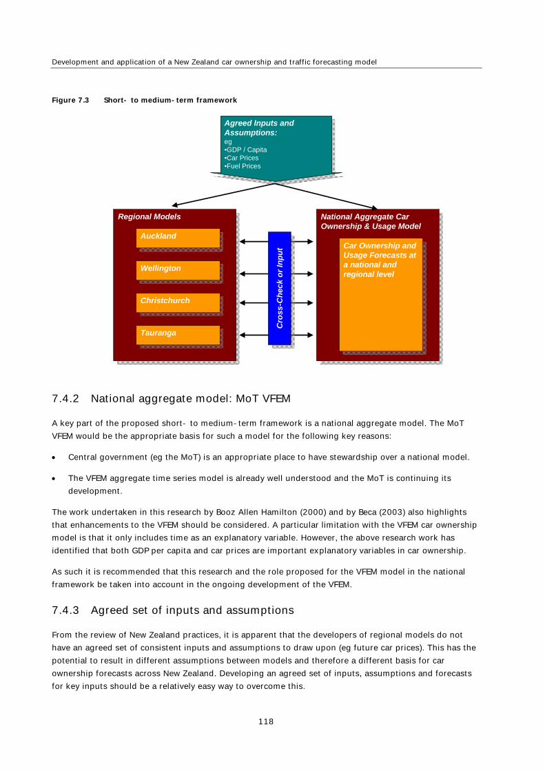
Development and application of a New Zealand car ownership and traffic forecasting model
118
Figure 7.3 Short- to medium-term framework
7.4.2 National aggregate model: MoT VFEM
A key part of the proposed short- to medium-term framework is a national aggregate model. The MoT
VFEM would be the appropriate basis for such a model for the following key reasons:
Central government (eg the MoT) is an appropriate place to have stewardship over a national model.
The VFEM aggregate time series model is already well understood and the MoT is continuing its
development.
The work undertaken in this research by Booz Allen Hamilton (2000) and by Beca (2003) also highlights
that enhancements to the VFEM should be considered. A particular limitation with the VFEM car ownership
model is that it only includes time as an explanatory variable. However, the above research work has
identified that both GDP per capita and car prices are important explanatory variables in car ownership.
As such it is recommended that this research and the role proposed for the VFEM model in the national
framework be taken into account in the ongoing development of the VFEM.
7.4.3 Agreed set of inputs and assumptions
From the review of New Zealand practices, it is apparent that the developers of regional models do not
have an agreed set of consistent inputs and assumptions to draw upon (eg future car prices). This has the
potential to result in different assumptions between models and therefore a different basis for car
ownership forecasts across New Zealand. Developing an agreed set of inputs, assumptions and forecasts
for key inputs should be a relatively easy way to overcome this.
Regional ModelsRegional Models
Agreed Inputs and Assumptions:eg•GDP / Capita•Car Prices•Fuel Prices
Agreed Inputs and Assumptions:eg•GDP / Capita•Car Prices•Fuel Prices
National Aggregate Car Ownership & Usage Model
National Aggregate Car Ownership & Usage Model
Car Ownership and Usage Forecasts at a national and regional level
Car Ownership and Usage Forecasts at a national and regional level
AucklandAuckland
WellingtonWellington
ChristchurchChristchurch
TaurangaTauranga Cro
ss-C
hec
k o
r In
pu
tC
ross
-Ch
eck
or
Inp
ut

7 Development of a recommended New Zealand modelling framework
119
7.5 Summary
The development of a static disaggregate model is the recommended car ownership and use modelling
methodology. This is because it provides the desired level of functionality identified in the needs survey
completed in this research. In particular a static disaggregate ownership model is able to test many policy
variables (eg public transport provision) and there is a large international body of experience to draw upon.
However it is recognised that developing a static disaggregate car ownership model for New Zealand is a
substantial undertaking and the development costs are likely to be significant. Consequently, there is
merit in exploring a short- to medium-term modelling framework. This framework would look to build
upon the MoT VFEM aggregate model to provide the basis for car ownership and use forecasts and to
ensure national consistency.

Development and application of a New Zealand car ownership and traffic forecasting model
120
8 Conclusions and recommendations
8.1 Conclusions
Examination of New Zealand car ownership and use data shows the following:
Car ownership in New Zealand has continued to increase. In 1970 car ownership was 0.310 cars per
person, by 2005 it had risen to 0.574 cars per person.
There appears to be a relationship between times of increasing GDP/person and decreasing car prices
corresponding to increased car ownership per person.
New Zealand continues to have one of the highest rates of car ownership in the world.
Information on vehicle kilometres travelled has been collected since 2001, using odometer readings
taken during the vehicle WoF inspections. This data shows that light vehicle travel per person
increased between 2001 and 2005, but decreased in 2006. Average annual travel per vehicle has been
decreasing since 2002.
Previous research has shows that increased petrol prices result in less fuel consumption per person.
An aggregate car model, previously developed by Booz Allen Hamilton (2000) has been updated as part of
this research. The following key conclusions have been made from its results:
The current level of car ownership in New Zealand, approximately 0.58 cars per capita, is below the
estimated saturation level of car ownership. The current saturation levels are estimated to be in the
range 0.67 cars per capita (lower) to 0.75 cars/capita (upper). By year 2041 the saturation level is
predicted to increase, due to changes in age distribution, to 0.71 cars per capita (lower) and 0.79 cars
per capita (upper).
Elasticities of GDP per capita and car price index can be used to predict future changes in car
ownership, particularly in the short to medium term. These appear to be a strong set of relationships.
There is considerable uncertainty over factors that could have a significant impact on car ownership.
For example it is unlikely that the real downward trend in the car price index will continue. The ability
to forecast future car ownership is dependent on the ability to accurately forecast changes in GDP and
car prices.
Economic conditions and car prices are predicted to have a significant impact on future car ownership.
Using the Booz aggregate model under the ‘high’ scenario, car ownership could reach the lower
estimate of saturation by approximately 2021.
The Booz aggregate model appears to perform better than the other examined New Zealand aggregate
models in the short-term (< 10 years). Over the medium term (10–20 years) the three models perform
in a similar manner.
A car ownership and use modelling ‘needs survey’ was conducted with transport practitioners in
New Zealand. The purpose of this survey was to examine the needs of users of car ownership and use
data. Conclusions drawn from this survey were used as an input to the development of a New Zealand car

8 Conclusions and recommendations
121
ownership and use modelling framework. They indicated that a modelling methodology for car ownership
and use should ideally:
be segmented by private vehicles (private and company ownership) and LCVs
be applied to national, regional, and local contexts
focus on forecasting within a 25-year horizon
segment vehicles by fuel type/efficiency and split between private and business
be sensitive to changes in fixed/variable costs, and in particular changes in fuel taxes and road user
charges, changes in income and the level of PT supply
have outputs that include vehicle numbers, usage, emissions and fuel consumption measures and to a
lesser extent, government revenue.
This review of New Zealand modelling practices and literature has identified the lack of a consistent
approach to forecasting car ownership in New Zealand. While some of the regional models are regulated
by national forecasts for car ownership, they are not the same forecasts. There does not appear to be a
consistent set of key input assumptions for these model forecasts (eg future GDP or income, car prices).
As these regional models are used to predict future transport requirements, the outputs forming an input
to project prioritisation, it would be highly desirable if the forecasting of car ownership was undertaken on
a consistent basis. As such, what appears to be lacking in New Zealand is an integrated framework for
forecasting car ownership.
The development of a national static disaggregate model is the recommended car ownership and use
modelling methodology. This is because it provides the desired level of functionality as identified in the
needs survey. In particular a static disaggregate ownership model is able to test many policy variables (eg
public transport provision).
However it is recognised that developing a static disaggregate car ownership model for New Zealand is a
substantial undertaking and the development costs are likely to be significant. Consequently, there is
merit in exploring a short- to medium-term modelling framework. This framework would look to build
upon the MoT VFEM aggregate model to provide the basis for forecasting car ownership and use, and
ensure national consistency.
8.2 Recommendations
The following actions are recommended for the transport sector:
To undertake a detailed review of the New Zealand Household Travel Survey and census data to ensure
these would meet the future requirements of a static disaggregate car ownership model. The travel
survey might need to be modified and should be undertaken on an annual basis.
To review definitions of vehicle ownership and classification used in census data, the household travel
survey and motor vehicle registration records with a view to achieving consistency throughout.
To implement a short- to medium-term framework for car ownership and use by:
- continuing development of the VFEM to strengthen it as a national car ownership and use model

Development and application of a New Zealand car ownership and traffic forecasting model
122
- developing a nationally consistent set of inputs, assumptions and forecasts for use in car
ownership at both the national and regional level
- encouraging developers and users of regional models to use the national car ownership model as
an input or cross-check of regional models (as appropriate).
To develop a static disaggregate car ownership and use model.
To review national guidelines for transport professionals to take into account changes in car
ownership and use when evaluating projects. Ideally these guidelines should be linked to the national
car ownership and use model.

9 References
123
9 References
Beca Carter Hollings & Ferner (Beca) (2003) Smartgrowth – car ownership forecasting. Prepared for
Smartgrowth, Tauranga.
Beca Carter Hollings & Ferner and Sinclair Knight Merz (Beca and SKM) (2003) Wellington transport
strategy model: TN15.1 car ownership report. Prepared for Greater Wellington Regional Council,
Wellington.
Booz Allen Hamilton (NZ) (1999) Wellington area transport strategic model report.
Booz Allen Hamilton (NZ) (2000) Model for forecasting vehicle ownership in New Zealand. Transfund NZ
research report 161.
Booz Allen Hamilton (NZ) (2007) Impacts of transport fuel price changes. Land Transport NZ research
report 331.
Bureau of Transport and Regional Economics (2002) Greenhouse gas emissions from transport, Australian
trends to 2020. Bureau of Transport and Regional Economics report 107.
Button, KJ (1974) A critical review of techniques used for forecasting car ownership in discrete areas. The
Statistician 23, no.2: 117–128.
Clark, LG (1982) The accuracy of economic roading evaluation. National Roads Board Road Research Unit.
Cited in Koorey et al (2000).
Cowi (1998) Energy efficiency from personal cars – possibilities for improvements through the tax
structure. (In Danish). Lyngby, Denmark: Cowi.
Cramer, JS (1959) Private motoring and the demand for petrol. Journal of the Royal Statistical Society:
334–47. Cited in Button (1974).
Dargay, J and D Gately (1999) Income’s effect on car and vehicle ownership, world wide: 1960–2015.
Transportation Research Part A: Policy and Practice 33, no.2: 101–138.
De Jong, G, J Fox, A Daly, M Pieters and R Smit (2004) Comparison of car ownership models. Transport
Reviews 24, no. 4: 379–408
Department of the Environment, Transport and Regions (DETR) (1997a) Car ownership: modelling and
forecasting. National road traffic forecasts (Great Britain) 1997 working paper no.1: 46pp.
Department of the Environment, Transport and Regions (DETR) (1997b) Car use: modelling and
forecasting. National road traffic forecasts (Great Britain) 1997 working paper no.2: 49pp.
Department of the Environment, Transport and Regions (DETR) (2001) Updating car ownership forecasts.
Final report. Institute for Transport Studies.
Department of the Environment, Transport and Regions (DETR) (2007) Updating national car ownership
model. MVA Consultancy.
Farrell, MJ (1954) The demand for motor cars in the United States. Journal of the Royal Statistical Society,
191-93. Cited in Button (1974).

Development and application of a New Zealand car ownership and traffic forecasting model
124
Hague Consulting Group (1989) Resource papers for Landelijk model, vol 2. Cited in De Jong et al (2004).
Hague Consulting Group and the Institute of Transport Studies (2001) Sydney strategic travel model: stage
1 estimation: estimation summary report. Report for New South Wales Department of Transport.
Hague Consulting Group and the Institute of Transport Studies (2002) Sydney strategic travel model: stage
1 estimation: further model estimation report. Report for New South Wales Department of Transport.
Hensher, DA and T Ton (2002) TRESIS: a transportation, land use and environmental strategy impact
simulator for urban areas. Transportation 29, no.4: 439–457.
Hensher, DA and WG Greene (2000) Choosing between conventional, electric and LPG/CNG vehicles in
single vehicle households. Prepared for the 9th World Conference of Transport Research, Seoul, July
2001.
Hounsell, N (1989) Limits to traffic growth in congested urban networks. TRRL Contractor Report 171.
Koorey, GG, TJ Mitchell, CM Fisk, SF Moynihan and ML Mara (2000) Traffic growth prediction. Transfund
NZ research report 191.
Kveiborg, O (1999) Forecasting developments of the car fleet in the Altrans model. Paper presented at the
Trafikdage på AUC conference. 30–31 August 1999.
Land Transport New Zealand (2006) Economic evaluation manual. Wellington.
Ministry of Transport (MoT) (1998) Vehicle fleet emissions model: New Zealand vehicle fleet database and
model development. Wellington: Ministry of Transport.
Ministry of Transport (MoT) (2007) The New Zealand light vehicle fleet: light fleet statistics 2007.
Wellington: Ministry of Transport.
OECD Factbook 2006 – economic, environmental and social statistics (2006),
http://oberon.sourceoecd.org/vl=1603667/cl=16/nw=1/rpsv/fact2006/
Ogut, KS (2004) S-curve models to determine car ownership in Turkey. The Bulletin of the Istanbul
Technical University 54, no.2.
Read, NSL (1971) The selection of data for economic appraisals of highway projects. National Roads Board
Road Research Unit. Cited in Koorey et al (2000).
Romilly, E, H Song and X Liu (1998) Modelling and forecasting car ownership in Britain: A cointegration
and general to specific approach. Journal of Transport Economics and Policy 32, part 2:165–185.
Stopher, P (2005) Challenges to using an integrated land-use transport model in Australia. Presentation at
the Oregon Integrated Models Symposium, November 2005.
Tanner, JC (1962) Forecasts of future numbers of vehicles in Great Britain. Roads and Road Construction:
263–74. Cited in Button (1974).
Tanner, JC (1965) Forecasts of vehicle ownership in Great Britain. Roads and Road Construction: 341–7.
Cited in Button (1974).
Tanner, JC (1966) Comments on ‘Forecasting car ownership and use’. Urban Studies: 143–5. Cited in
Button (1974).

9 References
125
Tanner, JC (1974) Forecasts of vehicles and traffic in Great Britain. Transport and Road Research
Laboratory report LR 650. Crowthorne: Transport and Road Research Laboratory.
Tanner, JC (1975) Forecasts of vehicles and traffic in Great Britain: 1974 revision. Transport and Road
Research Laboratory report LR 650. Crowthorne: Transport and Road Research Laboratory.
Tanner, JC (1977) Car ownership trends and forecasts. Transport and Road Research Laboratory report LR
799. Crowthorne: Transport and Road Research Laboratory.
Tanner, JC (1979) Choice of model structure for car ownership forecasting. Transport and Road Research
Laboratory report SR523. Crowthorne: Transport and Road Research Laboratory.
Tanner, JC (1983) A lagged model for car ownership forecasting. Transport and Road Research Laboratory
report LR 1070. Crowthorne: Transport and Road Research Laboratory.
Tanner, JC and AH Tulpule (1970) Recent work at the RRL on car ownership and forecasting. Car
ownership forecasting, PTRC Seminar Proceedings 5. Cited in Button (1974).
The Treasury (2007) Half year economic & fiscal update 2007. Wellington: The Treasury.
Whelan, G (2001) Methodological advances in modelling and forecasting car ownership in Great Britain.
Paper presented at the European Transport Conference 2001. Cambridge, UK.
Whelan, G, M Wardman and A Daly (2000) Is there a limit to car ownership growth? An exploration of
household saturation levels using two novel approaches. Paper presented at the European Transport
Conference 2000. Cambridge, UK.

Development and application of a New Zealand car ownership and traffic forecasting model
126
Appendix A: New Zealand vehicle ownership data
Table A.1 New Zealand vehicle ownership data (000)
NZ Yearbook licensed motor vehicles as at 31 March NZ Statistics licensed motor vehicles-Sept
quarter MoT
Year Cars Motorcycles Goods Other Total Cars Mcycs Goods Buses Total Lic veh to 31/12
1951 252.5 21.0 84.9 6.9 365.4 447.1
1952 282.0 26.7 95.2 7.0 410.9 494.2
1953 307.3 29.2 101.0 7.2 444.7 513.7
1954 325.3 29.7 103.0 7.3 465.3 553.5
1955 358.1 30.4 107.3 7.5 503.2 601.1
1956 395.5 28.8 115.2 7.7 547.1 638.3
1957 427.0 31.2 121.5 7.8 587.4 672.6
1958 464.6 33.9 115.3 7.8 621.7 702.9
1959 482.6 36.2 117.7 7.3 643.8 728.2
1960 504.8 36.8 119.4 7.2 668.3 762.7
1961 526.3 39.3 124.4 7.2 697.2 806.3
1962 555.8 44.4 130.2 7.5 737.8 844.1
1963 586.8 45.7 133.0 7.9 773.3 899.4
1964 633.3 46.9 138.3 7.6 826.1 963.9
1965 691.5 50.1 153.8 8.8 904.2 1013.8
1966 727.7 49.7 163.4 8.2 949.0 1060.2
1967 784.1 49.6 163.0 7.7 1004.5 1087.6
1968 810.9 48.4 164.7 7.7 1031.7 1114.7
1969 836.6 47.9 167.0 7.9 1059.3 1148.7
1970 865.2 48.0 171.5 7.8 1092.4 874.1 40.3 169.4 3.1 1086.8 1208.7
1971 911.9 53.1 181.8 7.4 1154.1 913.3 47.7 175.8 3.0 1139.9 1272.4
1972 959.5 62.9 190.6 7.3 1220.3 968.0 55.8 180.3 3.0 1207.0 1349.1
1973 1,025.0 72.4 194.7 7.3 1299.4 1029.5 63.6 187.3 3.0 1283.4 1438.8
1974 1,083.8 87.1 200.1 7.3 1378.4 1092.1 76.3 192.9 3.0 1364.4 1515.3
1975 1,134.9 93.7 206.8 7.6 1442.9 1134.0 83.4 194.6 3.1 1415.2 1574.5
1976 1,177.4 103.0 211.2 7.6 1499.2 1159.6 88.0 216.4 3.1 1467.2 1631.3
1977 1,205.9 107.0 232.2 7.7 1552.8 1181.9 85.5 221.3 3.2 1491.9 1642.8
1978 1,221.2 105.8 236.7 7.7 1571.3 1203.5 82.7 230.4 3.2 1519.9 1675.1
1979 1,250.2 106.5 247.9 7.7 1612.3 1239.9 95.8 235.6 3.2 1574.5 1732.9
1980 1,289.6 125.1 253.6 7.9 1676.2 1273.0 108.1 245.1 3.4 1629.6 1789.4
1981 1,325.4 138.5 264.5 8.0 1736.4 1308.5 113.5 257.3 3.3 1682.6 1846.1
1982 1,366.7 145.9 281.2 7.9 1801.8 1347.1 114.3 262.4 3.7 1727.4 1896.3
1983 1,401.2 145.4 288.0 7.5 1842.2 1378.3 112.6 270.9 4.0 1765.9 1921.5

Appendix A
127
Table A.1 New Zealand vehicle ownership data (000)
NZ Yearbook licensed motor vehicles as at 31 March NZ Statistics licensed motor vehicles-Sept
quarter MoT
Year Cars Motorcycles Goods Other Total Cars Mcycs Goods Buses Total Lic veh to 31/12
1984 1439.2 142.5 294.0 7.9 1883.6 1427.1 108.0 275.1 4.5 1814.8 1969.3
1985 1491.9 138.9 299.8 7.6 1938.2 1454.8 105.2 283.5 4.9 1848.4 1995.0
1986 1523.2 134.8 306.0 8.1 1972.1 2010.1
1987 2030.6
1988 1382.3 98.3 289.2 11.0 1780.8 1404.3 91.8 292.5 8.1 1796.8 2045.4
1989 1438.7 90.7 289.2 11.1 1829.7 1464.8 82.4 295.3 8.4 1850.9 2108.4
1990 1497.7 82.3 295.3 11.2 1886.5 1511.3 72.1 300.5 7.8 1891.8 2197.7
1991 1548.1 74.8 301.2 10.8 1934.8 1549.9 69.0 312.1 7.2 1938.2 2220.1
1992 1551.4 66.7 309.3 10.9 1938.2 1524.4 55.5 313.4 7.8 1901.0 2227.1
1993 1571.8 61.2 322.4 12.0 1967.4 1562.8 52.9 334.3 8.3 1958.4 2243.8
1994 1611.8 59.1 340.3 12.7 2023.9 1626.9 52.0 353.9 8.8 2041.7 2289.3
1995 1660.5 55.9 355.8 13.6 2085.8 1662.3 46.7 359.6 9.1 2077.8 2354.6
1996 1650.1 49.3 342.2 15.0 2056.6 1698.4 43.5 357.7 9.7 2109.3 2379.8
1997 1691.0 46.7 346.5 16.1 2100.4 1757.3 43.3 352.9 10.4 2163.9 2392.7
1998 1776.0 46.2 359.4 17.5 2199.1 1795.7 43.8 357.2 11.1 2207.8 2440.4
1999 1883.4 48.2 371.4 19.0 2322.0 1888.4 45.5 367.3 11.9 2313.2 2512.3
2000 1905.0 45.0 368.6 20.0 2338.7 1913.1 42.8 363.4 12.4 2331.7 2601.7
2001 1933.9 43.3 363.2 19.8 2360.1 1947.4 42.3 361.1 12.9 2363.6 2633.2
2002 1988.5 43.4 366.9 20.9 2419.8 1999.4 42.1 365.2 13.6 2420.2 2709.5
2003 2056.6 41.5 374.4 21.9 2494.3 2091.0 41.3 376.2 14.3 2522.8 2801.0
2004 2140.4 43.5 386.3 23.0 2593.2 2172.2 44.0 389.2 15.1 2620.5 2920.7
2005 2211.8 48.0 399.8 23.8 2683.5 2242.5 51.5 402.8 15.8 2712.5 3030.4
2006 2280.5 60.2 409.7 16.7 2767.1 3124.3

Development and application of a New Zealand car ownership and traffic forecasting model
128
Table A.2 Estimates of NZ motor vehicle ownership 1970–2006 (000)
Year Licensed vehicles
1 Sept quarter
Adjustment
factor
Booz & Company
estimate
1970 1086.8 0.99 1075.9
1971 1139.9 0.99 1128.5
1972 1207.0 0.99 1195.0
1973 1283.4 0.99 1270.6
1974 1364.4 0.99 1350.7
1975 1415.2 0.99 1401.0
1976 1467.2 0.99 1452.5
1977 1491.9 0.99 1476.9
1978 1519.9 0.99 1504.7
1979 1574.5 0.99 1558.7
1980 1629.6 0.99 1613.3
1981 1682.6 0.99 1665.8
1982 1727.4 0.99 1710.1
1983 1765.9 0.99 1748.2
1984 1814.8 0.99 1796.6
1985 1848.4 0.99 1829.9
1986 1859.3 0.99 1840.7
1987 1891.4 0.99 1872.5
1988 1796.8 1.05 1886.7
1989 1850.9 1.05 1943.4
1990 1891.8 1.05 1986.3
1991 1938.2 1.05 2035.1
1992 1901.0 1.05 1996.1
1993 1958.4 1.05 2056.3
1994 2041.7 1.05 2143.8
1995 2077.8 1.05 2181.6
1996 2109.3 1.05 2214.8
1997 2163.9 1.05 2272.1
1998 2207.8 1.05 2318.2
1999 2313.2 1.05 2428.8
2000 2331.7 1.05 2448.3
2001 2363.6 1.05 2481.8
2002 2420.2 1.05 2541.2
2003 2522.8 1.05 2648.9
2004 2620.5 1.05 2751.5
2005 2712.5 1.05 2848.1
2006 2767.1 1.05 2905.4
Notes:
(1) NZ Statistics September quarter (Table D.1)
(2) Figures for 1986 and 1987 estimated

Appendix A
129
Table A.3: New Zealand motor vehicle ownership 1970–2006
Year Cars (000) Motorcycles
(000)
Goods
(000)
Buses
(000)
Total
(000)
Population
mean
(000)
Cars
per
person
Motor-
cycles per
head
1970 865.3 39.9 167.7 3.0 1075.9 2788.9 0.310 0.014
1971 904.1 47.2 174.1 3.0 1128.5 2831.2 0.319 0.017
1972 958.3 55.2 178.5 3.0 1195.0 2876.0 0.333 0.019
1973 1019.2 63.0 185.4 2.9 1270.6 2931.3 0.348 0.021
1974 1081.2 75.6 190.9 3.0 1350.7 2993.6 0.361 0.025
1975 1122.7 82.6 192.7 3.1 1401.0 3057.8 0.367 0.027
1976 1148.0 87.1 214.2 3.1 1452.5 3111.3 0.369 0.028
1977 1170.1 84.7 219.1 3.1 1476.9 3136.2 0.373 0.027
1978 1191.5 81.9 228.1 3.2 1504.7 3143.5 0.379 0.026
1979 1227.5 94.8 233.2 3.2 1558.7 3143.1 0.391 0.030
1980 1260.3 107.0 242.6 3.4 1613.3 3138.0 0.402 0.034
1981 1295.4 112.3 254.8 3.3 1665.8 3146.7 0.412 0.036
1982 1333.6 113.1 259.8 3.7 1710.1 3161.2 0.422 0.036
1983 1364.6 111.4 268.2 4.0 1748.2 3189.5 0.428 0.035
1984 1412.8 107.0 272.4 4.5 1796.6 3230.6 0.437 0.033
1985 1440.3 104.1 280.6 4.9 1829.9 3259.3 0.442 0.032
1986 1451.7 105.2 278.1 5.8 1840.7 3273.3 0.444 0.032
1987 1478.4 102.7 285.3 6.1 1872.5 3281.6 0.451 0.031
1988 1474.6 96.4 307.2 8.5 1886.7 3310.2 0.445 0.029
1989 1538.0 86.5 310.1 8.8 1943.4 3318.3 0.463 0.026
1990 1586.8 75.7 315.5 8.2 1986.3 3336.5 0.476 0.023
1991 1627.4 72.5 327.7 7.5 2035.1 3373.1 0.482 0.021
1992 1600.6 58.2 329.1 8.2 1996.1 3415.8 0.469 0.017
1993 1641.0 55.6 351.0 8.7 2056.3 3452.0 0.475 0.016
1994 1708.3 54.6 371.6 9.2 2143.8 3491.1 0.489 0.016
1995 1745.5 49.0 377.6 9.6 2181.6 3539.3 0.493 0.014
1996 1783.3 45.6 375.6 10.1 2214.8 3618.3 0.493 0.013
1997 1845.2 45.4 370.6 10.9 2272.1 3747.3 0.492 0.012
1998 1885.5 46.0 375.1 11.6 2318.2 3792.2 0.497 0.012
1999 1982.8 47.8 385.7 12.5 2428.8 3821.9 0.519 0.013
2000 2008.7 44.9 381.6 13.0 2448.3 3842.9 0.523 0.012
2001 2044.7 44.5 379.1 13.5 2481.8 3867.5 0.529 0.011
2002 2099.3 44.2 383.4 14.3 2541.2 3899.6 0.538 0.011
2003 2195.6 43.4 395.0 15.0 2648.9 3970.0 0.553 0.011
2004 2280.8 46.2 408.7 15.8 2751.5 4044.9 0.564 0.011
2005 2354.6 54.1 422.9 16.6 2848.1 4101.3 0.574 0.013
2006 2394.5 63.2 430.2 17.5 2905.4 4148.0 0.577 0.015
Note: Figures for 1986 and1987 estimated

Development and application of a New Zealand car ownership and traffic forecasting model
130
Appendix B: Components of general model archetypes
Table B.1 General model types
MACRO
Aggregate (saturation)
time series models
Aggregate market
models
Heuristic
simulation
models
MICRO
Static disaggregate
ownership models
Indirect utility
models
COHORT
Cohort models or
panel models
Dynamic transaction
models
General
model
structure
The earliest models Tanner
(1958, 1962) fitted an ‘S-
curve’ as a function of time:
car ownership per capita
grew rapidly a moderate
levels of car ownership but
tapered off as car
ownership approached
saturation.
Later models such as
Tanner (1974) were
modified to incorporate
other explanatory variables
such as per capita income
and motoring costs. These
models implied that a
growth in income or
motoring costs could
‘speed up’ the approach
towards saturation.
However, it is important to
note that the eventual
‘saturation level’ of car
ownership is not affected
by income or motoring
costs – These variables only
influence the speed at
which saturation is
These models
simulate supply and
demand in the car
market (although
the focus is usually
on the used car
market).
The key driver these
models is the
scrappage model –
The scrappage
model predicts the
rate at which cars
are scrapped, based
on age and the price
of used cars.
The used car market
model is used to
determine the price
of used cars.
Other models are
used to predict
either the desired
stock of cars or new
car purchases.
These models
predict car
ownership, based
on heuristic
assumptions about
the proportion of
net income (after
expenses) that is
spent on cars.
In the FACTS
model, households
are assigned
desired kilometres
and they then
choose cars so as
to use up the
proportion of net
income available
for expenditure on
cars.
Low income
households may
be unable to
afford any cars,
while high income
These models
estimate the
probability of a
household owning
at least one car. This
estimate is influence
by characteristics of
the household,
including income
and household
structure.
They models also
estimate the
probability of a
household owning
more than one car,
given than that own
at least one car.
The estimations are
produced using
limited dependent
variable regression
models and cross-
sectional data.
These models
allow
households to
choose the
combination of
car ownership
and car use that
maximises their
utility
These models
generally group
and average
households into
age-based
cohorts. Each
cohort is treaded
as an observation
through time
Some models use
longitudinal data
of individuals
throughout time.
These models
generally estimate
car ownership
forecasts for each
cohort
These models predict
future ‘transactions’
(ie purchases and/or
disposal of cars)
These models begin
with current car
ownership patterns.
A duration model is
used to predict the
time (eg years) until a
household next
‘transacts’.
If a household does
not ‘transact’ then car
ownership is assumed
to be the same as it
was last year.
If a household does
‘transact’ then a type-
choice model will be
used to predict the
type of car purchased.

Appendix B
131
MACRO
Aggregate (saturation)
time series models
Aggregate market
models
Heuristic
simulation
models
MICRO
Static disaggregate
ownership models
Indirect utility
models
COHORT
Cohort models or
panel models
Dynamic transaction
models
approached.
The earliest models fitted
s-curves based on a logistic
function. However, other
researchers have employed
power function curves and
Gompertz curves.
households may
be able to afford
two cars.
Attributes
of model
Aggregate time series
models may be useful for
long-term predictions
because they focus on
‘saturations’.
However, these models
assume that the ‘end-state’
is the same, regardless of
intervening events (eg
people will eventually want
two cars per household,
regardless of what happens
to population density). This
assumption may not be
accurate.
In addition, these models
appear to implicitly assume
that the impact of
explanatory variables (such
as GDP per capita)
diminishes as households
get closer to saturation.
This appears to be a
reasonable approximation
Aggregate market
models are useful
for predicting the
composition of the
future car fleet
because they
incorporate
scrapping of used
cars
Therefore, these
models are useful
for predicting
energy consumption
and//ore emissions.
Heuristic
simulation models
exploit the
observed
consistency of the
proportion of net
income spent on
cars and car travel
Static disaggregate
models have two
main advantages:
1. These models use
cross-sectional
data, which avoids
issues with time
series data
2. These models
incorporate
characteristics (such
as household
structure) that are
likely to influence
car ownership and
use in the future.
Dynamic transaction
models are the
‘dynamic’ version of
static disaggregate
models – They enable
the use of
disaggregate models
in predicting type-
choice, without
assuming that
households can
choose a new car
instantaneously.

Development and application of a New Zealand car ownership and traffic forecasting model
132
MACRO
Aggregate (saturation)
time series models
Aggregate market
models
Heuristic
simulation
models
MICRO
Static disaggregate
ownership models
Indirect utility
models
COHORT
Cohort models or
panel models
Dynamic transaction
models
but, nevertheless, this
assumption should be
considered in assessment
of models.
Inputs
required
by the
model
Aggregate time series data:
average car ownership
rates
GDP per capita
other.
Assumptions about the
appropriate functional form
Aggregate data:
scrappage by
age and vehicle
type
used vehicle
prices by vehicle
type and
perhaps by age
imports and/or
vehicle stock by
vehicle type.
other.
Aggregate data:
household
expenditure on
cars and car
travel
vehicle prices.
Disaggregate car
ownership models
require cross-
sectional data on
household car
ownership and
explanatory
variables:
income
household
structure
location
other.
Disaggregate car
type ownership
models require
disaggregate data
collected from SP
and/or RP surveys.
Disaggregate
data collected
from SP surveys
Longitudinal data
and/or household
data that can be
aggregated into
cohorts
Disaggregate data
relating to household
vehicle choice data:
income
household
structure
location
other.

Appendix C
133
Appendix C: Model archetypes influencing factors
Economic growth
Static disaggregate models generally incorporate economic growth in the most sophisticated manner. For
example, the national road traffic forecasts (NRTF) model uses forecasts of income by household-type and
area to predict the probability of a household (in a particular household-type-area segment) owning a car.
Aggregate time series models incorporate economic growth into their models but only in a simple manner:
one of the key explanatory variables is forecast GDP per capita.
Heuristic simulation models also incorporate economic growth by making heuristic assumptions about the
relationship between net income and car purchases. However, the validity of these assumptions seems
questionable, especially for long-term forecasts, because the relationships between net income and car
purchases may change in the future.
Indirect utility models and dynamic transaction models also incorporate economic growth by incorporating
income as an explanatory variable. Cohort models and aggregate market models are designed to focus on
other aspects of car ownership.
Population and household size
Static disaggregate times series models and dynamic transaction models allow transport planners to
incorporate expected changes in household structure into forecast car ownership. This is a key advantage
of these models because household structure is likely to have an important influence on future car
ownership (eg future households are likely to have less children and more single-person households).
Furthermore, household structure is relatively easy to forecast so it is important that forecasts utilise this
information. Household structure can potentially also be incorporated into heuristic simulation models,
indirect utility models and cohort models.
However, models that use aggregate data, such as aggregate time series models and aggregate market
models cannot incorporate disaggregate data like household structure. This is a major disadvantage of
these models.
Age distribution and cohort effects
Cohort models are the only models that incorporate the impacts of generational trends in a comprehensive
manner. A key generational trend is the increased incidence of licence-holding amongst young females –
this will have implications for future car ownership.
These generational trends would appear to be an important influence on car ownership. Therefore, the
long-term forecasting ability of a car ownership model may be undermined if it does not incorporate a
licence-holding cohort model as an input into the main model. For this reason, the NRTF static
disaggregate ownership models uses a licence-holding cohort models as an input. The authors of the
Sydney STM static disaggregate ownership model mention that a licence-holding cohort model could be
developed as an input.

Development and application of a New Zealand car ownership and traffic forecasting model
134
The remaining models are more limited in their incorporation of age or ageing effects. In particular,
models that use aggregate data, such as aggregate time series models and aggregate market models
cannot incorporate disaggregate data like age.
Lag effects
The concept of lag effects is only applicable to aggregate time series models. Models with lag effects are
designed to reflect the time taken for changes in explanatory variables (eg petrol price changes, car price
changes) to feed through into car ownership patterns. Romilly et al (1998) found that the incorporation of
lag effects improved the forecasting performance of aggregate time series models considerably (see
Forecasting Performance for more information).
Saturation effects
Both the aggregate time series models and the static disaggregate models incorporate the concept of
‘saturation’.
However, the concept of ‘saturation’ underlying an aggregate time series model is quite different from the
concept of ‘saturation’ underlying a static disaggregate model. These differences are illustrated in the
table below:
Table C.1 Differences in concept of ‘saturation’
Saturation in aggregate time
series models
Saturation in disaggregate models (eg
NRTF)
Dependent variable Aggregate car ownership Proportion of households that own a car
Main explanatory variable Time
Income
Other key explanatory variables
GDP per capita
Household structure
Licence holding
Incorporation of saturation level
into model
The model assumes that there is
a saturation level for car
ownership.
The model assumes that the proportion
of households that own a car is between
zero and the saturation level (eg 80%)
Incorporation of saturation curve
into model
As time increases car ownership
follows a s-curve: early in an
economy’s development car
ownership grows rapidly, then it
diminishes towards saturation
As income increases, the probability of
owning a car follows an s-curve: at low
levels of income increases in income
have a big impact on the probability of
owning a car, but this effect diminishes
as income grows.
The table shows that the ‘saturation’ concept for aggregate time series models relates to car ownership
per capita, while the ‘saturation’ concept for static disaggregate models relates to the probability of a
household owning a car. Obviously, there are interlinkages between the two different concepts.

Appendix C
135
Factors influencing distance travelled
The following factors that affect car use were identified by the UK Department of Transport:
household income
composition of household and their location
changes in the level of car ownership including the proportions of single and multi car-owning
households
changes in fuel prices
change in fuel economy/efficiency.
The key determinants in car use were found to be income, the location and composition of households,
and the costs of motoring.
Car prices and fuel price changes
Disaggregate car ownership models do not generally incorporate car prices and fuel prices because they
are based on cross sectional data (ie a sample of people at a point in time). The UK Department for
Transport acknowledged that this was an unresolved difficulty of the 1997 NRTF model. In contrast,
aggregate time series models can incorporate car prices and fuel prices because they are based on time
series data (ie observations throughout time).
Some of the other models incorporate car prices (and sometimes also fuel prices): aggregate market
models and heuristic simulation models both have a strong focus on modelling the impact of car prices on
car purchases. Car prices could also be potentially incorporated into indirect utility models and dynamic
transaction models.
PT service and accessibility levels
Very few models incorporate PT service and accessibility levels. In particular, aggregate time series models
do not incorporate PT service or accessibility levels because they only use aggregate data.
There are a few exceptions. One exception is a static disaggregate model – the NRTF model – that
produces forecasts for different area-types (ie Greater London, Metropolitan districts and three other
categories with differing levels of population density) – This serves as a proxy for public transport
accessibility.
Data inputs
Aggregate time series models have the least demanding data input requirements. All these models require
is aggregate data on car ownership, GDP per capita, petrol prices, car prices, etc. Aggregate market
models and heuristic simulation models also have relatively low data requirements because they also use
aggregate data.

Development and application of a New Zealand car ownership and traffic forecasting model
136
Static disaggregate models and dynamic transaction models require more detailed data. These models
require a sample of households, along with data about each of these households including the number of
cars in the household, the number of licences, household income, etc.
Cohort models have one of the most demanding data input requirements. These models require
longitudinal data on individuals and/or household data that can be aggregated into cohorts.
Indirect utility models have to be estimated using disaggregate data collected from stated preference
surveys. The quality of this data is less than ideal because it is based on stated rather than revealed
preferences.
Model outputs
Aggregate time series models only produce estimates of car ownership per capita.
Cohort models predict single variables, such as car ownership per capita or incidence of licence holding,
amongst specific cohorts.
Dynamic transaction models and aggregate market models focus on the car stock as the key output. Both
of these models forecast based on the number of cars in use, the number purchased and the number
disposed.
Static disaggregate models and heuristic simulation models produce a richer set of predictions. These
models predict the number of households with no cars, one car and multiple cars. This information can be
used to forecast car use, using the number of vehicles in a household as an explanatory variable.
Forecasting performance
Research by Romilly et al (1998) explored the forecasting performance of a range of car ownership
models. The researchers compared the UK Department of Transport’s forecasts, which are based on a
static disaggregate model, with their own forecasts, which were based on a simple linear aggregate time
series model. The researchers found that the forecasts using the aggregate time series model were
superior.
References
Romilly, E, H Song and X Liu (1998) Modelling and forecasting car ownership in Britain: A cointegration
and general to specific approach. Journal of Transport Economics and Policy 32, part 2:165–185.

Appendix D
137
Appendix D: Summary of key model types
Aggregate (saturation) time series models Static disaggregate ownership models Aggregate market models
General model
structure
The earliest models Tanner (1962) fitted an ‘S-curve’
as a function of time: car ownership per capita grew
rapidly a moderate levels of car ownership but
tapered off as car ownership approached saturation.
Later models such as Tanner (1974) were modified
to incorporate other explanatory variables such as
per capita income and motoring costs. These models
implied that a growth in income or motoring costs
could ‘speed up’ the approach towards saturation.
However, it is important to note that the eventual
‘saturation level’ of car ownership is not affected by
income or motoring costs – These variables only
influence the speed at which saturation is
approached.
The earliest models fitted s-curves based on a
logistic function. However, other researchers have
employed power function curves and Gompertz
curves.
These models estimate the probability of a household
owning at least one car. This estimate is influence by
characteristics of the household, including income and
household structure.
These models also estimate the probability of a
household owning more than one car, given than that
own at least one car.
The estimations are produced using limited dependent
variable regression models and cross-sectional data.
Aggregate market models simulate supply
and demand in the car market (although the
focus is usually on the used car market). The
key driver in these models is a scrappage
model – the scrappage model predicts the
rate at which cars are scrapped, based on age
and the price of used cars. A used car market
model is used to determine the price of used
cars.
The key functionality of these models is that
they can be used to predict the composition
of the car fleet because they incorporate
scrapping of used cars. For example, the
scrappage model could be used to predict
when a significant amount of energy
inefficient vehicles are going to be retired.
Therefore, these models are useful for
predicting energy consumption and/or
emissions.
Variants/
supplementary
models
Dargay and Gately (1999) estimated Gompertz
functions using partial adjustment models. These
partial adjustment models enabled estimation of
short-run and long-run dynamics.
The car type choice model estimates the impact of
explanatory variables on the type of vehicle purchased.
These models predict the type of vehicle purchased as a
function of explanatory variables, such as household
income, vehicle prices, number of children and fuel costs.
These models are estimated using data from SP and RP
surveys.
There is variation in how vehicle scappage
and acquisition is modelled.

Development and application of a New Zealand car ownership and traffic forecasting model
138
Aggregate (saturation) time series models Static disaggregate ownership models Aggregate market models
National models
reviewed
CARMOD
NRTF
NRTF
STM
ALTRANS
TRESIS
Other national
models
LMS
VMM (car-type choice) for the UK
TREMOVE
Inputs required
by the model
Aggregate time series data:
Average car ownership rates
GDP per capita
other influencing factors (eg car prices).
Assumptions about the appropriate functional form
Disaggregate car ownership models require cross-
sectional data on household car ownership and
explanatory variables:
income
household structure
location
other.
Often data is collected from stated preference (SP)
and/or revealed preference (RP) surveys.
These models require aggregate data on the
car market, including the vehicle stock and/or
imports, scrappage rate and used vehicle
prices by vehicle type and perhaps by age.
(Dis)advantages
+ limited data requirements
+ dynamic
no or limited vehicle type distinctions
no or limited number of policy variables and
demographic distinctions
no car use.
+ behavioural foundation
+ many car types possible
+ many policy variables possible
large data requirements (but data on a household
level is often available
no car use (but can be included)
problems with shorter-time periods.
+ limited data requirements
+ both supply and demand side represented
static model
limited vehicle type distinctions
limited number of policy variables
no car use.

Appendix D
139
Aggregate (saturation) time series models Static disaggregate ownership models Aggregate market models
Outputs/
functionalities
Aggregate saturation models use time series data to
produce a forecast of a possible long-run saturation
level for car ownership per capita.
The models are limited in the sense that the long-
run saturation level is assumed independent of
income, fuel costs, etc. In particular, these models
assume that policy variables have no permanent
impact on ‘long-run’ car ownership. Saturation
models also produce forecasts for future
progression towards the saturation level.
The rate of progression towards the saturation level
is influenced by explanatory variables such as
income, etc.
The model is of limited use for traffic forecasting
because it only forecasts car ownership per capita –
The model does not distinguish between the number
of first, second and third cars, whereas this
distinction is important for forecasts of future traffic
levels.
Disaggregate ownership models predict the number of
households that own no cars, one car, two cars, etc.
A key functionality across all of the main disaggregate
ownership models is that they enable estimation of the
impact of income growth on car ownership. They do this
by looking at car ownership patterns across different
income groups, and then using that information to
extrapolate the impacts of income growth.
All of the main disaggregate ownership models also
enable estimation of the impact of household structure
on car ownership. However, different models represent
household structure in different ways
The Sydney STM also incorporates licence holding as an
explanatory variable. In addition the STM estimates
company car ownership separately.
None of the disaggregate ownership models reviewed
incorporate the impact of variables such fuel prices into
forecasts because they depend on the use of cross-
sectional data, rather than time series data.
Disaggregate car type models employ SP/RP data
relating to new vehicles cars purchased. Therefore, the
main functionality of car type models is in forecasting
the market share of each car type in new vehicle
forecasts.
Disaggregate car type models do not generally generate
the total number of new vehicles purchased so a
separate model is required to meet this functional need.
The key output from these models is
information about the vehicle fleet. These
models use aggregate data so they are unable
to relate car purchases to household
characteristics such as household structure.

Development and application of a New Zealand car ownership and traffic forecasting model
140
Aggregate (saturation) time series models Static disaggregate ownership models Aggregate market models
Outputs/
accuracy of
forecasts
The model’s forecasts will be relatively less accurate
because the forecasts use time series data –
Econometric analysis using time series data is often
less accurate that analysis using cross sectional
data, due to small sample size and autocorrelation.
In addition, the amount of confidence one can have
in ‘saturation’ levels is debated in the literature.
The model might produce accurate long-term
forecasts if one has confidence in the long-run
‘saturation’ level that is estimated.
The model may not be very effective at producing
short-term forecasts because it is so strongly based
around a long-term curve tracing toward saturation.
The forecasts from a disaggregate car ownership model
can be quite accurate because cross sectional data is
employed. This provides for a high sample size and
econometric issues with time series are avoided because of
random sample independence between observations.
The disaggregate models produce insightful long-term
forecasts because they incorporate long-run drivers of car
ownership, such as income and household structure.
One possible weakness of disaggregate models (in
terms of long-term forecasts) is that they do not
generally take into account drivers that can only be
measured with time series data, such as fuel costs.
Another possible weakness of disaggregate models is
that they make inferences about the effect of income on
car ownership by comparing car ownership across income
groups. However, some of the differences in car
ownership across income groups may be due to factors
other than just income (eg differences in attitudes).
The disaggregate models are relatively less effective at
short-term forecasts because the explanatory variables,
such as household structure, do not explain much of
short-term volatility in car ownership. Short-term
volatility in car ownership is caused primarily by variables
that are excluded from these models (car prices,
exchange rates, petrol prices, public transport prices).
The forecasts for car-type market share from
disaggregate car-type models are dependent on the
quality of SP/RP data. Research by Brownstone, Bunch
and Train (2000) suggests plausible forecasts require RP
data in addition to SP data.
The aggregate market models are particularly
useful in providing emissions forecasts as
they are able predict vehicle types (including
age, class, fuel) and vehicle use.
The weakness of this model type is that it is
effectively a static model. For example the
TREMOVE model is described as scenario
explorer as the equations used are
specifically designed to analyse changes in
behaviour as a result of changes in economic
conditions.

Appendix D
141
References
Brownstone, D, D Bunch and K Train (2000) Joint mixed logit models of stated and revealed preference for
alternative-fuel vehicles, Transportation Research Part B: Methodological 34, no.5: 315–338.
Button, KJ (1974) A critical review of techniques used for forecasting car ownership in discrete areas. The
Statistician 23, no.2: 117–128.
Dargay, J and D Gately (1999) Income’s effect on car and vehicle ownership, world wide: 1960-2015,
Transportation Research Part A: Policy and Practice 33, no.2: 101–138.
Tanner, JC (1962) Forecasts of future numbers of vehicles in Great Britain. Roads and Road Construction:
263–74. Cited in Button (1974).
Tanner, JC (1974) Forecasts of vehicles and traffic in Great Britain. Transport and Road Research
Laboratory report LR 650. Crowthorne: Transport and Road Research Laboratory.

Development and application of a New Zealand car ownership and traffic forecasting model
142
Appendix E: Review of international models
MODEL: Various
Reference
De Jong, G, J Fox, A Daly, M Pieters and Smit, R (2004) Comparison of car ownership models. Transport
Reviews 24, no.4: 379–408.
General forecasting model structure
The paper reviews nine types of car ownership models:
aggregate time series models
aggregate cohort models
aggregate car market models
heuristic simulation methods
static disaggregate car ownership models
indirect utility car ownership and use models
static disaggregate car-type choice models
(pseuo)-panel methods
dynamic car transactions models with vehicle type condition on transaction.
Aggregate time series models usually contain a sigmoid-type function of GDP per capita. The function that
increases slowly at low levels of GDP per capita, then rises steeply, then ends approaching a saturation
level. These models can be modified to incorporate fuel price levels, population density, road network
density, rail network density and time trends.
Aggregate cohort models segregate the current population into groups with the same birth year, and then
car ownership patterns for each of these cohorts. Certain cohorts have certain characteristics. For example,
the older generations grew up when a car-ownership lifestyle had not yet become firmly established;
therefore, this group retained relatively low rates of motorisation. In contrast, younger generations have
grown up during the ‘car era’ and can have more cars and can be expected to keep cars for longer.
Aggregate car market models distinguish between the demand and supply of cars in the car market. The
second-hand car-price is determined endogenously. The supply of new cars is generally assumed to be
perfectly elastic.
The TREMOVE model, as developed by KU Leuven and Standard & Poor’s DRI (1999) is an aggregate car
market model with three key components:
The first component determines transport flows by mode choice.

Appendix E
143
The second component describes how transport flows by mode choice, scrapping rates and car prices
affect car ownership by car-type.
The third component calculates emissions based on the number of kilometres driven by each vehicle.
The paper also discusses the ALTRANS model, which was described by Kveiborg (1999) and the TRESIS
model, developed by Hensher and Ton (2002) for Australian cities.
Heuristic simulation methods assume that households spend a constant proportion of net income on
transport. A discussion on evidence on these assumptions is provided in Schafer (2000).
The FACTS model, which was developed for the Netherlands, is provided as an example of a heuristic
simulation method. The model allocates business cars to households. The model then has households
picking car categories based on their household incomes. Households choose the most expensive car that
they can given their household incomes; the author points out that this is cost-maximising behaviour,
which is inconsistent with economic theory.
Static disaggregate car ownership models predict the number of cars owned by each household, generally
using binary logit models or similar empirical techniques.
The Dutch national model system (LMS), which is discussed by the Hague Consulting Group (1989) is an
early example of a static disaggregate car ownership model. This model first predicts licence holding, also
using disaggregate modelling. The model then uses licence holding to predict car ownership:
households with no licence will have no cars
household with one licence will choose between zero cars or one or more cars
households with two or more licences will choose between one car or two or more cars.
The decisions about number of cars owned in the LMS model are influenced by net monthly income (i.e.
income less expenditure on food, clothing and housing); therefore, if monthly income rises the probability
of car ownership increases. There is a fixed cost associated with car ownership; therefore, if fixed car
costs rise the probability of car ownership decreases.
The Sydney strategic transport model (STM), as described by the Hague Consulting Group (2000)
incorporates company car ownership into a static disaggregate car ownership model. In the Sydney STM,
the company car ownership model uses explanatory variables to predict the number of company cars
owned. It then uses a total car ownership model to predict the total number of cars in each household,
conditional on the number of company cars owned.
The UK Department for Transport modified its NRTF model to incorporate car ownership using a static
disaggregate car ownership model. First, the model predicts whether households have at least one car.
Then, if the model has at least one car, it predicts whether the household has two or more cars. The
model is influenced by a saturation level and licences per adult, household income and area type.
The NRTF model was later revised, based on an audit by Whelan (2001). An additional model was added
that estimated the probability of households having three or more cars. In addition, the model was
modified to allow single-person households to own more than one car; however, additional cars do not
impact on traffic forecasts because one person can only drive one car at a time.

Development and application of a New Zealand car ownership and traffic forecasting model
144
Indirect utility car ownership and use models integrate both car ownership and car use into an integrated
micro-economic framework.
De Jong (1989) developed two models that integrate car ownership and car use:
The first model – the ‘statistical model’ – assumes that a household has a structural desired annual
kilometrage, which depends on household income, household size, age, gender and occupation of the
head of the household. The household will own a car if the desired annual kilometrage exceeds a
certain threshold.
The second model – the ‘indirect utility model’ – allows households to compare combinations of car
ownership and car use and allows them to choose the combination with the highest utility. This
decision is influenced by both fixed car cost and variable car cost.
‘Indirect utility models’ were also developed by Train (1986), Hensher et al (1992) and for Norway’s
national model.
Norway’s national model is similar to the De Jong (1989) model, except that it has two components:
one component decides if the household has at least one car
another component decides if the household has one car or two cars (conditional on it having at least
one car).
The following variables were found to have a statistically significant impact on the number of cars chosen
in Norway’s national model: log of remaining household income, the variable cost of driving, the log of
household size and percentage urbanisation. The presence of a female head of household had a
significant impact on the first-car decision. The age of head of household (over 45 years, over 65 years)
also had an impact on the second-car decision.
Static disaggregate car-type choice models are similar to the models above, except that they also address
the choice of car-type in the household, given car ownership. These models are not discussed in detail in
the review of this paper because the research project is less concerned with car-type ownership.
(Pseudo) panel methods involve creating an artificial panel based on (cohort) averages of repeated cross-
sections. However, the averaging process means that information about individuals is lost because it is
captured in cohort means. The paper notes that, when defining cohorts, one should pursue homogeneity
within the cohorts and heterogeneity between the cohorts.
The research by Dargay and Vythoulkas (1995) is an example of pseudo panel methods. The researchers
broke the data down by five-year cohorts and by year between 1983–93, creating 165 pseudo-cohorts.
The dependent variable in the Dargay and Vythoulkas (1995) is the average number of vehicles per cohort,
while the explanatory variables included a lagged dependent variable, car purchase costs, car running
costs, public transport fares, income, the number of adults, the number of children, metropolitan and
rural areas and a generation effect for the head of the household. The only insignificant variables were
public transport fares and the number of children.
Dynamic car transactions models with vehicle type conditional on transaction model car purchase
decisions. For example, the Hocherman, Prashker and Ben-Akiva (1983) model allows a zero-car
household to choose to either purchase a new car or to do nothing. For a one-car household, the options
are replacement or do nothing.

Appendix E
145
Another example of a dynamic transaction model is the DVTM model developed by the Hague Consulting
Group (1993; 1995). The DVTM model also makes transaction decisions, which involve expanding or
replacing household vehicles. However, transactions are only made occasionally, and the time between
transactions is determined by a hazard-based duration model.

Development and application of a New Zealand car ownership and traffic forecasting model
146
Table E.1 Summary table
Aggregate time
series models
Aggregate
cohort models
Aggregate market
models
Heuristic
simulation models
Static
disaggregate
ownership
models
Indirect utility
models
Static
disaggregate
type choice
models
Panel models Pseudo-
panel models
Dynamic
transaction
models
General
structure
Most models use
a sigmoid-
shaped
‘saturation’
function to
predict car
ownership
These models
generally
estimate car
ownership
forecasts for each
cohort
These models
simulate the supply
and demand for cars
These models
assume that a
certain proportion
of net income (after
some expenses eg
food, rent) is spent
on cars.
Households on very
low incomes will be
unable to afford
any cars
These models first
estimate impacts
on the decision to
have at least one
car, then they
estimate the
number of cars
owned. At least
one model
incorporates
company car
ownership
These models allow
households to
choose the
combination of car
ownership and car
use that maximises
their utility
These models
address the
choice of car type
of the household,
given car
ownership
These models
use
longitudinal
data of
individuals
throughout
time
These models
group and
average
households
into age-
based
cohorts. Each
cohort is
treaded as an
observation
through time
These
models
predict
‘transaction
s’ (ie
purchases
and/or
disposal of
cars)
Underlying
theory
‘Saturation’ based
on product life-
cycle and
diffusion theories
Car ownership is
driven by forecast
licence-holding
within each
cohort
The supply of
existing cars (along
with cost and price
information)
influences new sales
of cars
The model is
heuristic because it
lacks underlying
theory and predicts
cost-maximisation
behaviour (which
contradicts
economic theory)
The model
assumes that
explanatory
variables affect
the decisions
about car
ownership
The model assumes
that households
maximise their utility
The model
assumes that
households
maximise their
utility
The number of
cars per
household is
assumed to
change over
time, as
explanatory
variables
change
The number
of cars per
household is
assumed to
change over
time, as
explanatory
variables
change
Car types No No Yes Yes No No Yes No No Sometimes
Dependent
variable
Car ownership
per capita
Car ownership
per capita (for
each cohort)
The number of
vehicles of each type
in the vehicle stock
The number of
vehicles in each
household, broken
down by vehicle-
type
The probability of
owning a car at
each stage of the
decision-making
process
Unestablished Unestablished The number of
cars per
household
The number
of cars per
household
Explanatory
variables
The main
explanatory
The main
explanatory
Inputs to the
simulation model
Inputs to the
simulation model
The explanatory
variables are net
The explanatory
variables considered
The explanatory
variables
The
explanatory
The
explanatory

Appendix E
147
Table E.1 Summary table
Aggregate time
series models
Aggregate
cohort models
Aggregate market
models
Heuristic
simulation models
Static
disaggregate
ownership
models
Indirect utility
models
Static
disaggregate
type choice
models
Panel models Pseudo-
panel models
Dynamic
transaction
models
variable is GDP
per capita, but
other variables
(population
density, fuel
prices) can also
be incorporated
variable is the
predicted number
of licences in
each cohort.
Other explanatory
variables include
income growth
per cohort
can include demand
for transport across
modes, the prices of
vehicles, and
scrapping rates.
only include
income, annual
kilometrage (see
below) and the
costs (fixed &
variable) associated
with each vehicle-
type
income (income
less expenditure
on food, housing
and clothing),
fixed car costs,
age, gender,
household size,
number of
workers in
household, and
region-specific
variables.
include fixed car
cost, variable car
cost, remaining
household income,
household size and
level of urbanisation.
The gender and age
of the head of the
household also had
an effect on
decisions
considered
include vehicle
attributes (price,
engine size, fuel
type, etc) and
household
attributes (gender
of head of
household,
number of
children, etc)
variables can
include socio-
economic
characteristics
of the
household
(income,
number of
adults,
number of
children, etc)
variables can
include socio-
economic
characteristics
of the
household
(income,
number of
adults,
number of
children, etc)
Cohort
effects
No Yes No No No, but age is an
explanatory
variable
No No Yes Yes No
Lag effects Yes ? No No Possible with time
series data
No No Yes Yes No
Saturation
levels
Yes Yes No No No No No No No No
Links to
traffic
modelling
None None The TREMOVE model
calculates transport
flows and modal
choice, and then
uses this information
to predict demand in
the car market.
The FACTS model
draws annual
kilometrage at
random from a
distribution and
uses this as an
input into the
model
These models
calculate both car
ownership and car
use simultaneously;
therefore, the car
use outputs can be
incorporated into
traffic modelling
These models are
used to describe
the composition
of the vehicle
fleet and are less
applicable to
traffic modelling
These models
can also
predict car
usage, but
only if data on
km driven is
available
These models
can also
predict car
usage, but
only if data on
km driven is
available
Empirical
techniques
Time series
analysis (eg artial
Unestablished Simulation model Simulation model Binary or
multinomial logit
Unestablished
Binary or
multinomial logit
Panel data
analysis
Panel data
analysis
Logistic
models are

Development and application of a New Zealand car ownership and traffic forecasting model
148
Table E.1 Summary table
Aggregate time
series models
Aggregate
cohort models
Aggregate market
models
Heuristic
simulation models
Static
disaggregate
ownership
models
Indirect utility
models
Static
disaggregate
type choice
models
Panel models Pseudo-
panel models
Dynamic
transaction
models
used adjustment
model)
models
The data can be
modelled using
ordered or
unordered
response choice
mechanisms
Bhat and
Pulugurta (1998)
recommend
unordered
response choice
mechanisms
models are used
to predict vehicle
choices, using
both SP and RP
data
used to
predict
‘transaction
s’
Hazard-
based
simulation
models
predict the
time
between
transactions
Features These models are
particularly
attractive for
application to
development
countries because
income is
considered to be
the driving
influence behind
car ownership
(and data
requirements are
low)
These models are
useful for
predicting the
impact of
population
changes on car
ownership
These models are
useful for estimating
impacts of car types
and, hence,
emissions
These models have
the limitation that
vehicle choice is
affected only by the
fixed and variable
costs associated
with each vehicle
category
These models have
the advantage that
they explain both car
ownership and car
use within the same
integrated
framework
These models are
primarily used to
predict the
composition of
the vehicle fleet
Examples TREMOVE model FACTS model UK NRTF model

Appendix E
149
MODEL: National road traffic forecasts (NRTF) – car ownership
References
Department of the Environment, Transport and Regions (1997) Car ownership: modelling and forecasting.
National road traffic forecasts (Great Britain) 1997 working paper no.1. 46pp.
Department of the Environment, Transport and Regions (2001) Updating car ownership forecasts. Final
report. Institute for Transport Studies.
Department of the Environment, Transport and Regions (2007) Updating national car ownership model.
MVA Consultancy.
General forecasting model structure
The UK Department of the Environment, Transport and Regions (DETR) developed both a car ownership
model and a car use model, which are then combined to create traffic forecasts.
There is, in effect, a car ownership model for each of the following household types:
one adult, not retired
one adult, retired
one adult, with children
two adults, retired
two adults, no children
two adults, with children
three-plus adults, no children
three-plus adults, with children.
DETR created ‘saturation’ levels for each of these household types. These ‘saturation’ levels were
influenced by both reasoning and analysis of licence data. For example, the model assumes that single
adult households will never own more than one car.
DETR used a three-step method to predict car ownership for each of the household types:
First, as noted above, the department created ‘saturation’ curves for each of the household types.
These ‘saturation’ curves predict the maximum proportion of households that own at least one car.5 It
then uses a logistic model to predict (in effect) where each household type is along their ‘saturation’
curve. Each household type’s position along their ‘saturation’ curve is affected by a utility of
ownership, based on explanatory variables (which is discussed below).
5 For example, the maximum proportion of one adult retired households that own at least one car is assumed to be 0.7

Development and application of a New Zealand car ownership and traffic forecasting model
150
Second, DETR created additional ‘saturation’ curves for the proportion of households owning two or
more cars, given that the household owns at least one car. Again, the household type’s position along
their ‘saturation’ curve is affected by a linear predictor of explanatory variables.
Third, DETR created additional ‘saturation’ curves for the proportion of households owning three or
more cars, given that the household owns at least two cars. Again, the household type’s position
along their ‘saturation’ curve is affected by a linear predictor of explanatory variables.
Forecasting model variables and their incorporation into model
The utility of ownership equations incorporate the following explanatory variables:
household income (by household type and area type)
number of adults employed
licences per adult
index of purchase costs
index of vehicle use costs
company cars.
The models are estimated using data from the Expenditure and Food Survey and the National Travel
Survey and relate the number of cars owned to:
socio-economic characteristics of the household
its geographical location
purchase and use costs
licence holding.
These explanatory variables are combined with car ownership ‘saturation’ assumptions and used to create
forecasts of car ownership by household types. The number of households within each household type is
also forecast (using demographic forecasts). These are combined with the forecasts of car ownership by
household types – the resulting forecasts reflect a prediction of car ownership in the future.
Table E.2 Forecasting model variables and their incorporation into model
Component Content
Economic growth or
income growth
The GDP or ‘income’ is included as an explanatory variable (and is modified
by household-type and area)
The report notes that distribution of ‘income’ is also important, but is
assumed to be unchanged into the future, for the purposes of forecasting.
Population and household
size
The number of households (broken down by household type) is forecast
using demographic forecasts.
Cohort effects The car ownership model does not directly include cohort effects. However,
the saturation levels are set with regard to cohorts. Also, the forecasts for
future licences per adult were based on analysis of cohorts.
Time trend effects There are no explicit time trend variables but a method was adopted which
forecasts ‘year specific constants’ into the future, by relating them to the

Appendix E
151
Component Content
projected growth in licence holding.
Lag effects There are no lag effects
Saturation effects There are saturation effects in this model – the assumed ‘saturation’ rates
constrain the forecast car ownerships. For example, single-adult households
are assumed to only have either no car or one car; similarly, only 70% of
single-adult retired households are assumed to ever have a car.
Car price and fuel price
effects
Car purchase prices and use costs are explanatory variables.
PT service and
accessibility effects
The are no explicit allowances for PT. However, the area type discussed
below may serve as a proxy for accessibility to PT services because the area
types reflect differing population densities.
Region effects The model allows the impact of ‘income’ on car ownership to differ by area
type. Five area types are incorporated:
Greater London
Metropolitan districts
districts with density 10+ persons per hec.
districts with density 2 to 10 persons per hec.
districts with density 0 to 2 persons per hec.
Trends in distance
travelled per car
Car use is discussed in working paper 2.
Linkages between car ownership model and traffic models
Forecasts for car ownership and forecasts for car use (ie kilometres per car) are combined together to
create traffic forecasts.
Approaches to forecasting at national, regional and sub-regional/local levels
The model is capable of producing forecasts for each of the five area-types discussed earlier.
Application of the model
The model is implemented and is used for the NRTF.
MODEL: NRTF – car use
Reference
Department of the Environment, Transport and Regions (1997) Car use: modelling and forecasting.
National road traffic forecasts (Great Britain) 1997 working paper no.2. 49pp.
General forecasting model structure
This model focuses on forecasting car use (defined as the average annual distance travelled per car).
The forecasting process consists of three stages:

Development and application of a New Zealand car ownership and traffic forecasting model
152
Stage 1 – incorporate elasticities of car use with respect to income, broken down by household
type and car ownership patterns
Stage 2 – incorporate an aggregate elasticity of car use with respect to changes in fuel costs
Stage 3 – refine model using company car adjustment
During stage 1, DETR estimated the elasticities of car use with respect to income using cross-sectional
data from the 1991/93 National Travel Survey. However, the car use forecasts produced using stage 1 had
no regard to the impact of fuel costs (fuel prices and fuel efficiency) on car use. Therefore, during stage 2,
DETR estimated fuel cost elasticities using an error correction model. DETR then used the error correction
model to project two series for car use forecasts: one series included assumptions about future fuel costs;
the other series assumed that fuel costs stayed constant. The difference between these two series was
used to adjust the forecasts from stage 1. During stage 3, the forecasts from stage 2 were modified using
a company car adjustment. This adjustment was made to ensure that the proportion of company cars in
the car stock (and the consequent effects on kilometres driven) did not increase disproportionately as the
number of multi-car-owning households increased.
The general form of the resulting equation is:
(Equation E.1)
adjustment
car
company
x
households
carowning
numberof
arforecastye
xomeuseholdincbaseyearho
oldincomeyearhousehforecastx
effecttfuel
milageyearbase densityIncomehousehold
carnumberof
j
typehouseholodeach
icos
sin
Table E.3 Forecasting model variables and their incorporation into model
Component Comment
Economic growth or
Income growth
The cross sectional car use model (from stage 1) uses forecast income, by
household type and car ownership, as an input into the model.
The paper notes that there is a clear relationship between income and car-
use – the relationship is almost linear – there is no evidence of a ‘saturation’
effect, as there is with car ownership.
Population and household
size
The cross sectional car use model incorporates forecasts for numbers of
people in each household type. For example, the number of one adult,
retired households was forecast to rise by 135% from 1996 to 2031.
Cohort effects The car use models do not explicitly incorporate cohort effects but they use
forecasts of numbers of people in each household type, which may be based
on cohort analyses.
Time trend effects There are no time trend effects.
Lag effects There are no lag effects
Saturation effects There are no saturation effects
Car price and fuel price
effects
The time series model (from stage 2) estimates the impact of fuel cost (fuel
price and fuel efficiency) on car use.
PT service and
accessibility effects
Proximity to bus services and proximity to rail services were included in
cross-sectional analyses of 1991–93 National Travel Survey data.
However, these variables were not used in the final cross sectional model.
The reasons for this are not stated, but the empirical output shows that the

Appendix E
153
Component Comment
coefficients on these variables were often counter-intuitive.
Region effects The paper claims on paragraph 8 that location is incorporated into the car
use model, but there is no evidence elsewhere of this, including in the
empirical output.
Trends in distance
travelled per car
The paper notes that car use has generally growth. However, there have been
periods of decline (1973–79, 1990 onwards) which can generally be
associated with shocks to the price of fuel, and lower growth in GDP.
Linkages between car ownership model and traffic models
The car use forecasts are combined with the car ownership forecasts to produce forecasts for total traffic.
Estimates of parameters produced
Car use in Great Britain, measured in annual kilometres per car, has grown from an average of 13,860km
in 1951 to 15,970km in 1996. It was also identified that in the 20 years up to 1996, there was an
increased in the proportion of shorter journeys and the average car trip length increased.
The following table provides the household elasticities from the model:
Figure E.1 Household elasticities of car use with respect to income, and average kilometres per car
Approaches to forecasting at national, regional and sub-regional/local levels
The method does not appear to vary by region.
Application of the model
The model is implemented and is used for the NRTF.

Development and application of a New Zealand car ownership and traffic forecasting model
154
Model: CARMOD
Reference
Bureau of Transport and Regional Economics (BTRE) (2002) Greenhouse gas emissions from transport,
Australian trends to 2020. Bureau of Transport and Regional Economics report 107,
General forecasting model structure
The Bureau of Transport and Regional Economics (BTRE) developed the CARMOD model for the purpose of
forecasting car fuel use. Previous versions of CARMOD calculated total vehicle numbers as the product of
population and vehicle ownership – vehicle ownership was assumed to follow a simple logistic function
over time. However, GDP growth and decreases in real vehicle prices have encouraged higher car
ownership levels than that implied by the older model, as depicted in the following figure.
Figure E.2 Projected car ownership in Australia
Notes: ‘Old fit’ refers to projected values used in BTCE Report 94 (BTCE 1996b).
‘New fit’ refers to revised estimates allowing for price and income effects (including the recent surge in vehicle sales).
CARMOD has been revised to take into account the surge in vehicle ownership experienced over the past
five ears. It is now based on a function that relates total private vehicle travel to real income growth. Car
ownership rates are then derived using forecast VKT per person and forecast VKT per car.
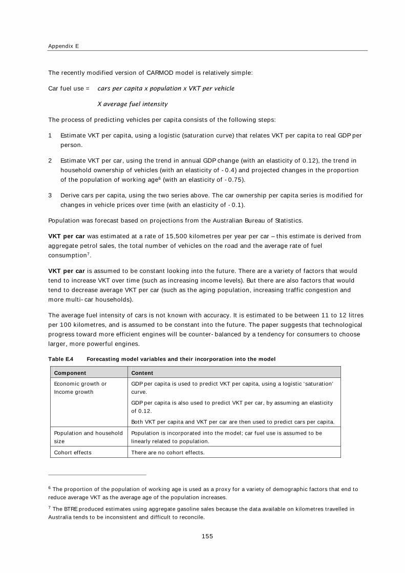
Appendix E
155
The recently modified version of CARMOD model is relatively simple:
Car fuel use = cars per capita x population x VKT per vehicle
X average fuel intensity
The process of predicting vehicles per capita consists of the following steps:
1 Estimate VKT per capita, using a logistic (saturation curve) that relates VKT per capita to real GDP per
person.
2 Estimate VKT per car, using the trend in annual GDP change (with an elasticity of 0.12), the trend in
household ownership of vehicles (with an elasticity of -0.4) and projected changes in the proportion
of the population of working age6 (with an elasticity of -0.75).
3 Derive cars per capita, using the two series above. The car ownership per capita series is modified for
changes in vehicle prices over time (with an elasticity of -0.1).
Population was forecast based on projections from the Australian Bureau of Statistics.
VKT per car was estimated at a rate of 15,500 kilometres per year per car – this estimate is derived from
aggregate petrol sales, the total number of vehicles on the road and the average rate of fuel
consumption7.
VKT per car is assumed to be constant looking into the future. There are a variety of factors that would
tend to increase VKT over time (such as increasing income levels). But there are also factors that would
tend to decrease average VKT per car (such as the aging population, increasing traffic congestion and
more multi-car households).
The average fuel intensity of cars is not known with accuracy. It is estimated to be between 11 to 12 litres
per 100 kilometres, and is assumed to be constant into the future. The paper suggests that technological
progress toward more efficient engines will be counter-balanced by a tendency for consumers to choose
larger, more powerful engines.
Table E.4 Forecasting model variables and their incorporation into the model
Component Content
Economic growth or
Income growth
GDP per capita is used to predict VKT per capita, using a logistic ‘saturation’
curve.
GDP per capita is also used to predict VKT per car, by assuming an elasticity
of 0.12.
Both VKT per capita and VKT per car are then used to predict cars per capita.
Population and household
size
Population is incorporated into the model; car fuel use is assumed to be
linearly related to population.
Cohort effects There are no cohort effects.
6 The proportion of the population of working age is used as a proxy for a variety of demographic factors that end to
reduce average VKT as the average age of the population increases.
7 The BTRE produced estimates using aggregate gasoline sales because the data available on kilometres travelled in
Australia tends to be inconsistent and difficult to reconcile.

Development and application of a New Zealand car ownership and traffic forecasting model
156
Component Content
Time trend effects There was a time-trend effect in the previous version of CARMOD, but this
has been abandoned in favour of a model that is related more to GDP per
capita.
Lag effects There are no lag effects.
Saturation effects A saturation effect is assumed for the relationship between VKT per capita
and GDP per capita; therefore, a logistic ‘saturation’ model is used to model
this relationship.
Car price and fuel price
effects
Car price is incorporated into the model because the forecasts for cars per
capita was modified based on forecasts for car prices and an assumed
elasticity of -0.1.
PT service and
accessibility effects
There are no PT service effects.
Region effects There are no region effects.
Trends in distance
travelled per car
The paper does point out the surprising surge in car ownership for the five
years leading up to 2000. This was attributed to GDP growth and decreases
in real vehicle prices.
Linkages between the car ownership model and traffic models
In a sense, the CARMOD model begins with traffic model variables (VKT per capita, VKT per car) and it
uses these to derive car ownership (ie cars per capita). The cars per capita variable is then used, in
conjunction with other variables, to predict total fuel use. This approach is confusing, especially since VKT
per capita is already calculated and seems to remove any need to estimate cars per capita.
Empirical/MR techniques for estimating parameters
The logistic relationship between VKT per capita and GDP per capita was estimated using Australian data.
The elasticities for the forecasts of other variables were estimated, where possible, using regression
analyses on BTRE long-term data sets for Australian vehicle characteristics. Where this was not possible,
elasticities were based on the literature.
Estimates of parameters produced
VKT per car with respect to GDP: 0.12
VKT per car with respect to ‘the trend in household ownership of vehicles’: -0.4
VKT per car with respect to the proportion of population of working age: 0.75
VKT per car with respect to fuel price changes: -0.1
Cars per capita with respect to vehicle prices: -0.1
Approaches to forecasting at national, regional and sub-regional/local levels
The model is national.

Appendix E
157
Application of the model
The model has been implemented and is used for predicting future emissions from the transport sector.
Critique and commentary
The BTRE initially estimated the relationship between VKT per capita and GDP per capita.
The most efficient method of calculating total fuel use would be to combine VKT per capita, total
population and fuel efficiency.
However, the BTRE appears to use a less efficient method:
VKT per car is also estimated
VKT per car and VKT per capita are used to estimate cars per capita
Cars per capita, VKT per car, population and fuel efficiency are all used to estimate total fuel use.
Model: ALTRANS
Reference
Kveiborg, O (1999) Forecasting developments of the car fleet in the Altrans model. Paper presented at the
conference Trafikdage på AUC. August 30-31st 1999.
General forecasting model structure
The Altrans (ALternative TRANSport systems) model was developed at the National Environmental
Research Institute (DMU) in Denmark for the purpose of forecasting energy consumption and emissions
from personal transport. The Altrans model has a car stock sub-model that consists of three different
parts:
Tt = Tt-1 + Nt - St
Where: Tt = existing stock of cars
Nt = acquisitions
St = scrapping.
The car stock sub-model uses existing information on the stock of cars from Statistics Denmark. This
information is also used to calculate estimates for scrappage. The level of scrappage is calculated for cars
broken down by fuel-type, weight and age. These breakdowns are all considered important because these
attributes all influence emissions. A ‘scrappage model’ is used to estimate the level of scrappage in the
future (St). Scrappage is assumed to be a function of various exogenous variables, including income and
price indices for fuel, acquisitions and repairing costs.
The acquisitions of new cars (Nt) is assumed to be the difference remaining after the stocks and
scrappages above are estimated.

Development and application of a New Zealand car ownership and traffic forecasting model
158
Table E.5 Forecasting model variables and their incorporation into model
Component Content
Economic growth or Income growth Income is an explanatory variable
Population & household size Population is not an explanatory variable
Cohort effects No cohort effects
Time trend effects No time trend effects
Lag effects No lag effects, but predictions of future stocks are based around
current stock levels
Saturation effects No saturation effects
Car price and fuel price effects The price of fuel and acquisitions (of cars) are both included in
the model as explanatory variables
PT service and accessibility effects Not included
Region effects Not discussed
Trends in distance travelled per car Not discussed
Linkages between car ownership model and traffic models
The models described above are used to estimate future vehicle stocks.
The ‘behavioural model’ is also used to estimate the absolute level of driven kilometres. This absolute
level of driven kilometres is then apportioned out to the vehicle stock, using information on the average
distance driven by cars of certain ages.
Empirical/MR techniques for estimating parameters
Maximum likelihood is used to predict the impact of fuel type, weight and age on scrapping in each of the
120 categories.
Estimates of parameters produced
The paper does not discuss parameter estimates.
Approaches to forecasting at national, regional and sub-regional/local levels
The paper indicates that the model is only used for national forecasting
Application of the model
The model has been implemented and is used to prediction national emissions.

Appendix E
159
Model: TRESIS
Reference
Hensher, DA and T Ton (2002) TRESIS: A transportation, land use and environmental strategy impact
simulator for urban areas. Transportation 29, no.4: 439–457.
With supporting evidence from:
Stopher, P (2005) Challenges to using an integrated land-use transport model in Australia. Presentation at
the Oregon Integrated Models Symposium, November 2005.
General forecasting model structure
The transportation and environment strategy impact simulator (TRESIS) was developed to assist transport
planners in making predictions about the impact of transport strategies.
TRESIS contains a number of discrete choice models:
household location and type of dwelling
work locations for household workers
number and type of vehicles owned by the household
levels of use of vehicles by trip purpose
means of travel by departure time.
This review focuses on the discrete choice models for the number and type of vehicles owned by the
household. There are 10 size classes for conventional fuel vehicles (micro, small, medium, upper medium
1, upper medium 2, large, luxury, light commercial, four wheel drive and light trucks). There is also
capacity for including vehicles based on alternative fuels. Vehicles are also distinguished by age.
TRESIS predicts automobile fleet size and vehicle type mix choice conditional on commuter mode,
departure time choice and residential locations. More information on these models can be found in
Hensher and Ton (2002).
TRESIS can model vehicle ownership using two alternative methods:
The vehicle price relativity approach:
In the vehicle price relativity approach, new vehicle prices are exogenous. Used vehicle prices are
predicted based on new vehicle prices, using a non-linear empirical equation. This approach ensures a
relativity between new vehicle prices and used vehicle prices. The scrappage rate is predicted as a function
of vehicle age and used vehicle prices.
The supply of new vehicles is determined as the difference between total household demand for new
vehicles and the supply of used vehicles (which is affected by scrappage).

Development and application of a New Zealand car ownership and traffic forecasting model
160
The equilibration approach
In the equilibration approach, new vehicle prices are also exogenous. However, used vehicle prices are
determined by equilibrium. As with the vehicle price relativity approach, the scrappage rate is a function of
age and value.
Total demand for vehicles (by class) is determined by vehicle choice and fleet size models. The difference
between demand and scrappage gives the number of new vehicles by class.
Table E.6 Forecasting model variables and their incorporation into model
Component Content
Economic growth or
Income growth
Income is not explicitly mentioned as an explanatory variable
Population and household
size
Population and household size are not explicitly mentioned as an
explanatory variable.
However, the impact of residential density on household behaviour, such as
kilometres driven, can be estimated.
Cohort effects Cohort effects are not discussed.
Time trend effects Time trend effects are not discussed
Lag effects Lag effects are not discussed
Saturation effects Saturation effects are not discussed, but the behavioural models that
determine car choice possibly incorporate plausible assumptions about the
number of cars owned by households.
Car price and fuel price
effects
Vehicle prices are exogenous explanatory variables in the model so the
impact of vehicle price changes on the vehicle fleet could be explored.
Fuel prices are not discussed as an explanatory variable for car ownership,
but they are an explanatory variable in the wider TRESIS model.
PT service and
accessibility effects
PT service and accessibility are not explicitly mentioned as an explanatory
variables for car ownership. However, modal share is an output variable in
the TRESIS model – so PT service is incorporated into the TRESIS model in
some manner.
Region effects The TRESIS prototype was developed to be applicable to the Sydney
Metropolitan Area. It was also been applied in South Australia and the paper
notes that it can be applied to six urban areas.
Trends in distance
travelled per car
These are not discussed.
Linkages between car ownership model and traffic models
The TRESIS model is integrated so it incorporates both car ownership and travel demand.
Empirical/MR techniques for estimating parameters
This is not discussed.
Estimates of parameters produced
This is not discussed.

Appendix E
161
Approaches to forecasting at national, regional and sub-regional/local levels
The TRESIS model is region-specific. It contains a lot of detail that appears to be specific to the region of
interest.
Application of the model
The model has been developed and applied in South Australia.
Model: STM
Reference
Hague Consulting Group and the Institute of Transport Studies (2001) Sydney strategic travel model: stage
1 estimation: estimation summary report. Report for New South Wales Department of Transport.
Hague Consulting Group and the Institute of Transport Studies (2002) Sydney strategic travel model: stage
1 estimation: further model estimation report. Report for New South Wales Department of Transport.
General forecasting model structure
The Sydney strategic travel model (STM) consists of the following sub-models:
1 A model to predict licence holding by household
2 A model to predict car ownership, conditional on licence-holding
3 A model to predict the frequency of trips to work, by employed individuals
Model for licence holding
In Sydney, from 1971 to 1998, licence holding increased from 62% to 81%.
About four fifths of this increase in licence holding can be attributed to a ‘catching up’ of women’s licence
holding relative to men’s licence holding. This occurred because of a gradual replacement of generations
of women who had low licence holding by younger women whose licence holding has always been very
similar to men’s. This ‘catching up’ effect has been the main driver of changes in licence holding over the
last 20 years. The effect will probably continue to be a major driver of licence over the next 20 years.
However it may be dampened by immigration from countries where women’s licence holding is generally
low.
Many car ownership models include a ‘trend’ variable representing increasing car ownership that cannot
be explained by income. This ‘trend’ can be attributed, at least in part, to a growth in licence holding.
Therefore, it is important that projections into the future take into account the impact of licence holding.
Cohort analysis could be used to forecast licence holding for the future, but it is not in the Sydney STM.
However, the accuracy of those forecasts will depend on information on immigration from South
American, African and Asian countries.
The Sydney STM predicts the likelihood of households being in one the following four states:
neither member of household has a licence

Development and application of a New Zealand car ownership and traffic forecasting model
162
head of household has a licence; partner does not have a licence
head of household does not have a licence; partner does have a licence
both head of household and partner have a licence
Households are more likely to have licences as income increases, the number of children increases and
with the presence of employment. Households are less likely to have licences if the head of the household
is female, the head of the household is under 25 or over 70 or if the household is large.
Model for car ownership:
First, the Sydney STM company car ownership model predicts the probability of households having the
following:
no company cars
1 company car
2 company cars.
The predictions of the company car ownership model are influenced by (the log of) household income, the
number of licences in the household, the ages of the household members and the presence of a female
head of household.
The Sydney STM total car ownership model then predicts the probability of households having the
following:
0 cars
1 cars
2 cars
3 or more cars
The predictions of the total car ownership model are influenced by (the log of) household income, the
number of licences in the household, the ages of the household members, the presence of company cars,
and the employment status (part-time, full-time) of the members of the household. Interestingly, in the
total car model, the income term is reduced by the average car ownership for the cars owned by the
household.
Model for travel frequency
The Sydbey STM for travel frequency predicts the number of trips to work for employed individuals. The
first stage of the travel frequency model predicts whether any work ‘tours’ will be made. The second stage
of the model predicts whether more than one ‘tour’ will be made each day due to, for example, a second
job. The travel frequency model is influenced by age dummies, gender, the presence of a licence, income,
manufacturing employment and employment status (eg full-time, part-time, casual).

Appendix E
163
Table E.7 Forecasting model variables and their incorporation into model
Component Content
Economic growth or
Income growth
Household income is an explanatory variable in the car ownership models
and in the travel frequency model.
Population and household
size
Prototypical sampling was employed – The sample was ‘re-weighted’ to
reflect future populations.
Cohort effects Cohort effects were discussed and presented in graphs, but were not
incorporated into the model.
Time trend effects These were not employed, and the use of time trends in other car ownership
models was criticised.
Lag effects These were not discussed.
Saturation effects There was no saturation function, but the models used to predict car
ownership only allow up to three cars. Furthermore, the number of cars is
influenced by licence-holding.
Car price and fuel price
effects
Car prices and fuel prices do not affect the number of cars owned in the
model.
PT service and
accessibility effects
PT service accessibility does not affect the number of cars owned in the
model.
Region effects The model is designed to be applicable to the Sydney region.
Trends in distance
travelled per car
These are not discussed in detail.
Linkages between car ownership model and traffic models
The initial models predict car ownership and this is used as an input for predicting the frequency of travel
to work and the times of the day in which travel to work occurs.
Empirical/MR techniques for estimating parameters
The models were all estimated using cross sectional data.
Estimates of parameters produced
The parameter estimates are provided in appendices A, B and C of the Hague Consulting Group and the
Institute of Transport Studies (2002) report.
Approaches to forecasting at national, regional and sub-regional/local levels
The model is designed to be applicable to the Sydney region.
Application of the model
The model is implemented.
References
Bhat, C and V Pulugurta (1998) A comparison of two alternative behavioural choice mechanisms for
household auto ownership decisions, Transportation Research Part B: Methodological 32, no.1: 61–75.

Development and application of a New Zealand car ownership and traffic forecasting model
164
Bureau of Transport and Regional Economics (BTRE) (2002) Greenhouse gas emissions from transport,
Australian trends to 2020. Bureau of Transport and Regional Economics report 107.
Dargay, J.M and PC Vythoulkas (1999) Car ownership in urban and rural areas: a pseudo panel analysis.
London: ESRC Transport Studies Unit, Centre for Transport Studies, University College London.
De Jong, GC (1989) Simulating car cost changes using an indirect utility model of car ownership and car
use. Paper presented at PTRC SAM. Brighton UK, 1989.
De Jong, G, J Fox, A Daly, M Pieters and R Smit (2004) Comparison of car ownership models. Transport
Reviews 24, no.4: 379–408.
Department of the Environment, Transport and Regions (DETR) (1997) Car ownership: modelling and
forecasting. National road traffic forecasts (Great Britain) 1997 working paper no.1. 46pp.
Department of the Environment, Transport and Regions (DETR) (1997) Car use: modelling and forecasting.
National road traffic forecasts (Great Britain) 1997 working paper no.2. 49pp.
Department of the Environment, Transport and Regions (DETR) (2001) Updating car ownership forecasts.
Final report. Institute for Transport Studies.
Department of the Environment, Transport and Regions (DETR) (2007) Updating national car ownership
model. MVA Consultancy.
Hague Consulting Group (1989) Resource papers for Landelijk model, vol. 2. Cited in De Jong et al (2004).
Hague Consulting Group (1993) Een gedisaggregeerd model van bezitsduur, typekeuze, jaarkilometrage
en brandstofverbruik van personeauto’s. Report 319–1. The Hague: Hague Consulting Group.
Hague Consulting Group (1995) Further development of a dynamic vehicle transactions model. Report
5037–1. The Hague: Hague Consulting Group.
Hague Consulting Group (2000) Sydney car ownership models. Report 9009–3B. The Hague: Hague
Consulting Group.
Hague Consulting Group and the Institute of Transport Studies (2002) Sydney strategic travel model: stage
1 estimation: further model estimation report. Report for New South Wales Department of Transport.
Hensher, D.A. and T Ton (2002) TRESIS: a transportation, land use and environmental strategy impact
simulator for urban areas. Transportation 29, no.4: 439–457.
Hensher, DA, PO Barnard, NC Smith and FW Milthorpe (1992) Dimensions of automobile demand: a
longitudinal study of vehicle ownership and use. Amsterdam: North Holland.
Hocherman, I, JN Prashker and M Ben-Akiva (1983) Estimation and use of dynamic transaction models of
automobile ownership. Transportation Research Record 944: 134–141.
KU Leuven and Standard and Poor’s DRI (1999) Auto-oil II cost effectiveness: study description of the
analytical tools TREMOVE 1. Second draft, working document. Leuven: KU Leuven en Standard and
Poor’s DRI.
Kveiborg, O (1999) Forecasting developments of the car fleet in the Altrans model. Paper presented at the
Trafikdage på AUC conference. 30–31 August 1999.

Appendix E
165
Schafer, A (2000) Regularities in travel demand: an international perspective, Journal of Transportation
and Statistics 3, no.3: 1–32.
Train, K (1986) Qualitative choice analysis: theory, econometrics and an application to automobile
demand. Cambridge, MA: MIT Press.

Development and application of a New Zealand car ownership and traffic forecasting model
166