Carleton University

STAT5703W Data Mining I

Research Project

Partial Least Squares

Authors: Mounika Reddy, Kamran Karim, Olga Shumeyko

March 26, 2018

Statement of the Responsibilities:

1. Mounika Reddy: In detail explanation about the steps to perform, functions to be used in PLS

and Real time applications of PLS, Summary.

2. Kamran Karim: Performing a literature review of the topic, introducing PLS as a feature

extraction technique and explaining in theory how PLS works.

3. Olga Shumeyko: application of Partial Least Square analysis to gasoline dataset, R code.

Contents Introduction .................................................................................................................................................. 4

Feature Extraction ......................................................................................................................................... 5

Principle Component Regression .................................................................................................................. 5

Partial Least Squares Regression .................................................................................................................. 6

Algorithm to use:[1] .............................................................................................................................. 6

Real life Applications of Partial Least Squares .............................................................................................. 7

Example using PLSR ....................................................................................................................................... 8

Fitting models ............................................................................................................................................. 12

Number of Latent Variables to Use: ................................................................................................... 12

Analysing the Quality of Prediction: ................................................................................................... 12

Inspecting Fitted models ............................................................................................................................. 13

Plotting ................................................................................................................................................ 13

Predicting new observations....................................................................................................................... 14

Summary ..................................................................................................................................................... 14

References .................................................................................................................................................. 15

Appendix A – R code ................................................................................................................................... 16

Introduction In this report we will introduce a popular method of dimension reduction. Dimension reduction in

statistical modelling, refers to reducing the number of input variables (to reduce complexity of the

model), by forming linear combinations of the original predictor variables and using the new linear

combinations, instead of the original variables to predict the response variable(s). The need of such

reduction of dimension is sometimes because of high correlation between the predictor variables,

sometimes for interpretability, i.e. reducing the number of variables give us more information about the

relations between the dependent and independent variables and finally sometimes it is needed just to

be able to run a regression, as the sample size is small compared to the number of predictor variables,

that we cannot run the full model as is. The new variables that are created from the original predictor

variables are called “Latent Variables”, and there are various ways to achieve these Latent Variables, not

all of which would give us the same result. This whole class of technique is known as Structural Equation

Modeling (SEM), which comprises of many different techniques to perform the Latent variable analysis.

The SEM techniques can be divided into two main areas, first is the Covariance-based SEM and the other

is the Variance-Based SEM, the Covariance one being more general, is the more generalizable of the

two, but due the easiness of implementation and some other benefits that we don’t see in the

covariance-based technique (due to complexity and assumptions) the variance-based is very widely

used. In the variance based SEM, the most widely used technique is the Principle Component Regression

(PCR). A more generalized case of PCR is the Partial Least Squares or Projection on Latent Structures

(either way PLS) Regression. In this report we will have our focus on this technique more than any else,

we will use some other known techniques, as to compare with the PLS, which will help understand PLS

better. The report will be consisting of three sections, the first section will comprise of the definition of

PLS and supporting Literature, in the following section we give examples of where the topic is being

used, and in the final section we will give an example by taking some raw data and implementing the

technique to realise the relation between the dependent and independent variables. Note that for a

greater understanding of this report we would try to be as less technical in our approach as possible, in

the context we would try to explain stuff using what is known and avoid the use of too much

mathematics in our approach.

Feature Extraction Feature Extraction is a method that leads to the dimension reduction of data, where the p predictors are

projected to the M-dimensional space (where p<M, i.e. dimensions decrease in number). The ways it is

achieved is by calculating M different linear combinations of the original p predictor variables. Once the

M new latent variables (as defined in the introduction) are achieved, a linear regression model by least

squares is applied on these new latent variables to seek the relation between dependent and

independent variables.1

There are mainly two kinds of approaches for feature extraction, first is the unsupervised, the most

common one used is the Principle Component Regression, where as the one for supervised is the Partial

Least Squares. Before we get into explaining the Partial Least squares, it might be beneficial to put some

main features of the Principle component analysis, which is the reader might be more familiar with and

then introduce PLS by comparing it with the former.

Principle Component Regression By far the Principle Component Analysis/Regression (PCA/PCR)2 is the most common type of dimension

reduction, is a feature extraction method that is viewed as a special kind of scoring method under the

Singular Value Decomposition3 or SVD (method using orthogonal linear projections to capture

underlying variance of data). The main assumption that PCR makes is that the way data shows variation

in the predictor variables is the same way data shows variation in the predicted variables (dependent

variables). The idea behind its usage is to use as less variables as possible that shows the most variation

of the response variables. Using this idea, PCR chooses the top M combinations of predictor variables,

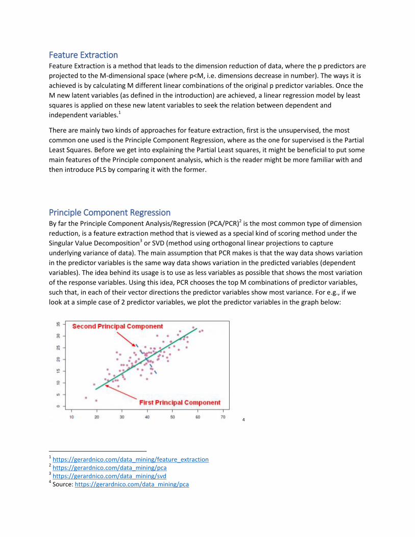
such that, in each of their vector directions the predictor variables show most variance. For e.g., if we

look at a simple case of 2 predictor variables, we plot the predictor variables in the graph below:

4

1 https://gerardnico.com/data_mining/feature_extraction

2 https://gerardnico.com/data_mining/pca

3 https://gerardnico.com/data_mining/svd

4 Source: https://gerardnico.com/data_mining/pca

In the figure above we see that most variation in the predictor variables is shown in the direction that is

labelled as First Principal Component, whereas after taking this into account the next direction that

shows maximum variance and is also orthogonal (90 ) to the first component is the dashed line.

According to our assumption, these two directions will give us the paths in which the response variable

varies the most, but the response variable itself is not used to determine these directions, and for this

report this might be the most noteworthy point, the question why will be answered later in the report.

Note that from how we have defined the latent variables, the more the predictor variables are

correlated with each other, the better the new latent variable helps in the explaining the response

variable.

Partial Least Squares Regression Partial Least Square Regression is another technique that comes under the umbrella of variance-based

SEM, and just like PCR, the PLSR also does the SVD technique, i.e. the latent variable found are

orthogonal to each other. That is, it is almost similar to the PCA except for the fact that it doesn’t make

the assumption that the variation in the predictor variables is mimicked in the variation in the response

variables. So unlike the Principal components method the Partial least squares take into account the

value of the response variables along with that of the predictor variables, in order to calculate the latent

variables. Hence, this method can be seen as more generalised than the former. Similar to other

methods in the set of techniques to perform dimension reduction or feature extraction, the PLS is also

used either when the number of predictor variables is too large, and hence to reduce this number or if

there is high multicollinearity between predictor variables. The way PLS achieves this is by searching for

the latent vectors that perform a simultaneous decomposition of X and Y with the constraint that these

components explain as much as possible of the covariance between X and Y.

Algorithm to use:[1]

PLS regression decomposes X and Y as a product of a common set of orthogonal factors and a specific

set of loadings. The independent variables are decomposed as with , where I is the

identity matrix, T is the score matrix and P is the loading matrix. Similarly, Y is estimated as ,

where left hand side is the prediction and B is a diagonal matrix with regression weights, and C is the

weight matrix of dependent variables. Now the latent variables can be found in a lot of different ways, in

essence we have to find two sets of weights w and c, such that the linear combinations of columns of X

and Y have the highest covariance. The first pair of such vector obtained is denoted by:

With constrains and . Than the t vector found is the first latent vector

found is subtracted from X and from Y to get X’ and Y’. Now the same process is reiterated on X’ and Y’

to get the second latent vector. The process goes on until X matrix becomes null.

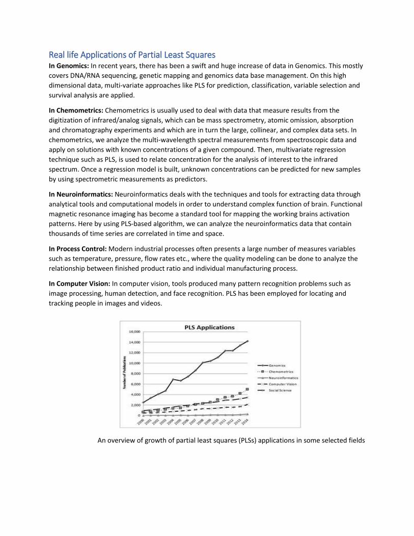
Real life Applications of Partial Least Squares In Genomics: In recent years, there has been a swift and huge increase of data in Genomics. This mostly

covers DNA/RNA sequencing, genetic mapping and genomics data base management. On this high

dimensional data, multi-variate approaches like PLS for prediction, classification, variable selection and

survival analysis are applied.

In Chemometrics: Chemometrics is usually used to deal with data that measure results from the

digitization of infrared/analog signals, which can be mass spectrometry, atomic omission, absorption

and chromatography experiments and which are in turn the large, collinear, and complex data sets. In

chemometrics, we analyze the multi-wavelength spectral measurements from spectroscopic data and

apply on solutions with known concentrations of a given compound. Then, multivariate regression

technique such as PLS, is used to relate concentration for the analysis of interest to the infrared

spectrum. Once a regression model is built, unknown concentrations can be predicted for new samples

by using spectrometric measurements as predictors.

In Neuroinformatics: Neuroinformatics deals with the techniques and tools for extracting data through

analytical tools and computational models in order to understand complex function of brain. Functional

magnetic resonance imaging has become a standard tool for mapping the working brains activation

patterns. Here by using PLS-based algorithm, we can analyze the neuroinformatics data that contain

thousands of time series are correlated in time and space.

In Process Control: Modern industrial processes often presents a large number of measures variables

such as temperature, pressure, flow rates etc., where the quality modeling can be done to analyze the

relationship between finished product ratio and individual manufacturing process.

In Computer Vision: In computer vision, tools produced many pattern recognition problems such as

image processing, human detection, and face recognition. PLS has been employed for locating and

tracking people in images and videos.

An overview of growth of partial least squares (PLSs) applications in some selected fields

Example using PLSR The function plsr and dataset gasoline presented here are from pls package [2]. The pls package

implements Partial Least Squares Regression (PLSR) in R.

First the package should be loaded:

library(pls)

gasoline - dataset consisting of octane number (octane) and NIR spectra (NIR) of 60 gasoline

samples [3]. Each NIR spectrum consists of 401 diffuse reflectance measurements from 900 to 1700 nm

(see ?gasoline).

plsr(formula, ncomp, data) – is the simplest form to call plsr function. Where parameter formula is a

formula that consist of a left hand side (representing the response), a tilde (~), and a right hand side

(representing the predictors); ncomp is the number of components, and data is the data frame

containing the variables to use in the model. There are other parameters as well.

We did PLSR on gasoline data to illustrate the use of PLSR. First, we loaded the dataset:

data(gasoline)

Then we divided the dataset into train and test datasets: gasTrain and gasTest.

We called plsr function on train data set and 10 components and leave-one-out (LOO) cross-validated predictions:

pls.gas1 <- plsr(octane ~ NIR, ncomp = 10, data = gasTrain, validation = "LOO")

summary(pls.gas1) Data: X dimension: 45 401 Y dimension: 45 1 Fit method: kernelpls Number of components considered: 10 VALIDATION: RMSEP Cross-validated using 45 leave-one-out segments. (Intercept) 1 comps 2 comps 3 comps 4 comps 5 comps 6 comps 7 comps 8 comps 9 comps 10 comps CV 1.464 1.319 0.5358 0.2303 0.2172 0.221 0.2226 0.2296 0.2357 0.2525 0.2738 adjCV 1.464 1.319 0.5337 0.2286 0.2168 0.220 0.2215 0.2271 0.2320 0.2501 0.2721

TRAINING: % variance explained 1 comps 2 comps 3 comps 4 comps 5 comps 6 comps 7 comps 8 comps 9 comps 10 comps X 68.85 79.37 85.09 95.46 96.15 96.77 97.01 97.33 98.22 98.83 octane 26.81 89.50 98.07 98.44 98.82 99.01 99.15 99.24 99.29 99.36

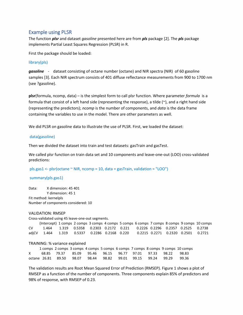
The validation results are Root Mean Squared Error of Prediction (RMSEP). Figure 1 shows a plot of

RMSEP as a function of the number of components. Three components explain 85% of predictors and

98% of response, with RMSEP of 0.23.

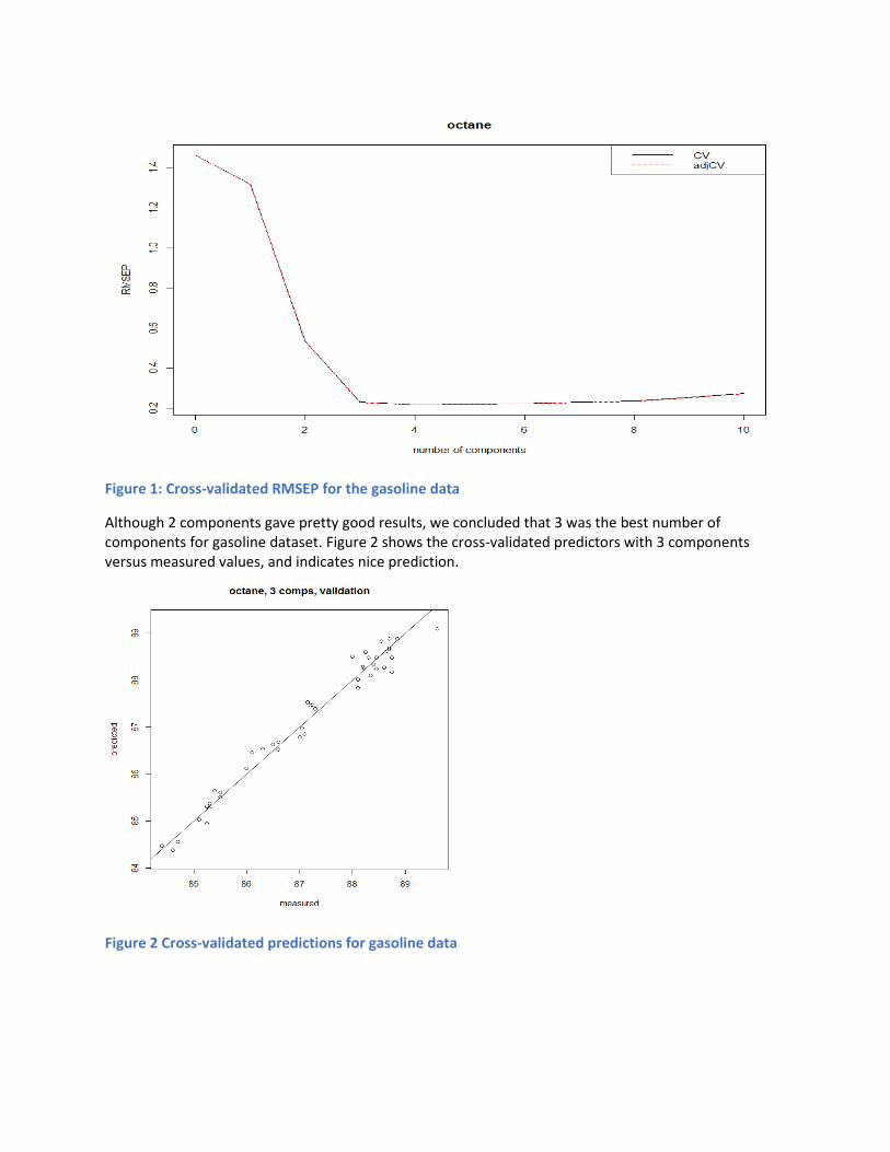
Figure 1: Cross-validated RMSEP for the gasoline data

Although 2 components gave pretty good results, we concluded that 3 was the best number of components for gasoline dataset. Figure 2 shows the cross-validated predictors with 3 components versus measured values, and indicates nice prediction.

Figure 2 Cross-validated predictions for gasoline data

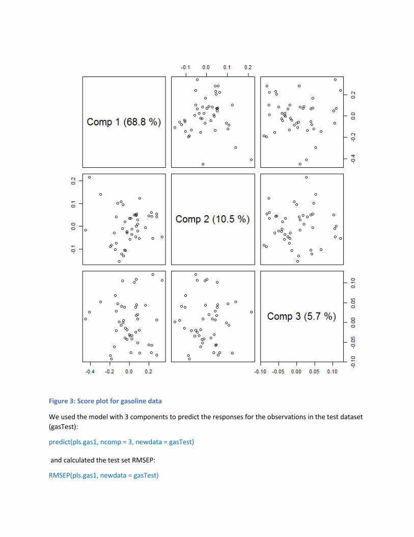
Figure 3: Score plot for gasoline data

We used the model with 3 components to predict the responses for the observations in the test dataset

(gasTest):

predict(pls.gas1, ncomp = 3, newdata = gasTest) and calculated the test set RMSEP:

RMSEP(pls.gas1, newdata = gasTest)

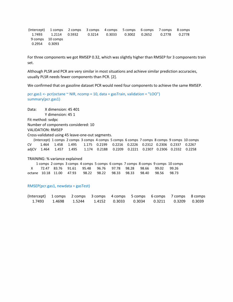
(Intercept) 1 comps 2 comps 3 comps 4 comps 5 comps 6 comps 7 comps 8 comps 1.7493 1.2114 0.5932 0.3214 0.3033 0.3002 0.2652 0.2778 0.2778 9 comps 10 comps 0.2954 0.3093

For three components we got RMSEP 0.32, which was slightly higher than RMSEP for 3 components train

set.

Although PLSR and PCR are very similar in most situations and achieve similar prediction accuracies,

usually PLSR needs fewer components than PCR. [2].

We confirmed that on gasoline dataset PCR would need four components to achieve the same RMSEP.

pcr.gas1 <- pcr(octane ~ NIR, ncomp = 10, data = gasTrain, validation = "LOO") summary(pcr.gas1) Data: X dimension: 45 401 Y dimension: 45 1 Fit method: svdpc Number of components considered: 10 VALIDATION: RMSEP Cross-validated using 45 leave-one-out segments. (Intercept) 1 comps 2 comps 3 comps 4 comps 5 comps 6 comps 7 comps 8 comps 9 comps 10 comps CV 1.464 1.458 1.495 1.175 0.2199 0.2216 0.2226 0.2312 0.2306 0.2337 0.2267 adjCV 1.464 1.457 1.495 1.174 0.2188 0.2209 0.2221 0.2307 0.2306 0.2332 0.2258

TRAINING: % variance explained 1 comps 2 comps 3 comps 4 comps 5 comps 6 comps 7 comps 8 comps 9 comps 10 comps X 72.47 83.76 91.61 95.48 96.76 97.78 98.28 98.66 99.02 99.26 octane 10.18 11.00 47.93 98.22 98.22 98.33 98.33 98.40 98.56 98.73

RMSEP(pcr.gas1, newdata = gasTest) (Intercept) 1 comps 2 comps 3 comps 4 comps 5 comps 6 comps 7 comps 8 comps 1.7493 1.4698 1.5244 1.4152 0.3033 0.3034 0.3211 0.3209 0.3039

Fitting models The main functions for fitting models are pcr and plsr. We will use both plsr and pcr and compare their

results below.

Syntax for Fitting models: plsr (formula, ncomp, data, validation) (the same syntax applies to pcr as

well). Where,

ncomp: number of components one chooses to fit.

data: Data frame containing variables to use in the model.

Validation: it is for sending arguments to the underlying functions, (i.e.) to a cross-validation function

mvrCv.

The above function returns a fitted model which can be used for predicting new observations. In the

above function, if the argument ncomp is not provided then maximum possible number of components

is used. Also data is optional and if it is missing, it can be searched for in the user’s workspace. But It is

usually preferred to keep the variables in data frames, in that case we have to use formulas like

octane~NIR and have to specify the data frame with data=gasTrain as below.

Fitting model when applied to our gasoline data set:

pls.gas1<-plsr (octane~NIR, ncomp=10, data=gasTrain, validation=”LOO”). This scatter corrects NIR prior

to the fitting, and this makes the new spectra to be automatically scatter corrected, since we use the

same reference spectrum in predict as well. Below is the syntax for predict.

predict (pls.gas1,ncomp=3,newdata=gasTest)

Number of Latent Variables to Use:

The quality of model does not always strictly increase with the increase in the number of latent

variables in the PLS techniques, typically, the quality first increases and then decreases after a certain

number of additions of variables. If the quality is decreasing, it means that we maybe over fitting the

data and taking away the aspect of generalisability of the model, if all latent variables of X are used than

we are not really doing anything it’s a simple regression model. When only a subset of the variables is

used, the prediction of Y is optimal for this number of predictors. To look at the optimal number of

variables to choose, please refer to the article by Herve Abdi (2010) [1], page 5, which talks about the

theory behind the optimal choice of number of these latent variables.

Analysing the Quality of Prediction:

In a fixed effects model, i.e. where the set of observations is considered the population of interest (and

not just a sample), here the latent variables shall have a meaning full interpretation, i.e. one shall be

able to explain the relation that comes out in the form of an equation. Here the overall quality of the PLS

regression model using L latent variables is evaluated by first computing the predicted matrix of

dependent variables and then comparing it with the original matrix Y. The most popular such

comparison is called Residual sum of squares and is defined as:

The lower the RRES the better the model is. For a fixed effects model, the higher the value of L is the

better is the model.

In contrast to the fixed effects model in a random effects model (where the observations are just a

sample from the population of interest, hence the goal is to build a model that can later be used to

better predict the new observations. Techniques like bootstrap or jackknife can be used to find the

appropriate number of latent variables which will give the best model. Once again, the reader is referred

to look at Abdi (2010) [1] to look at the details for this section to know more theory behind it.

Now we will give a quick comparison of the PCR and the generalised technique PLS. Note that both

techniques serve two basic purposes in the regression, first is to convert highly correlated variables to a

set of independent variables using linear transformations and secondly both lead to variable reductions.

The main difference between the two techniques is the fact that PLS is supervised, and explains

comparatively more variation in Y, given same number of latent variables chosen for both the

techniques. Note that usually the assumption that we make for PCA, i.e. the variation in the predictor

variables mimic that of the response variable, almost holds, hence the results from each technique

might have very similar results, but theoretically the PLS has some edge over the PCA technique for

regressions.[1]

Inspecting Fitted models

Plotting

All plotting functions can be accessed through “plottype” argument of the plot method for mvr objects.

This is simply a wrapper function calling the actual plot functions. PLS package has number of plot

functions for plotting cross-validated predictions, scores, loading and correlation loading. A detailed

explanation for each kind of the plottype is given below:

Prediction plot (predplot): It is used for showing predicted versus measured values. Predictions are

made according to the data set that is fed to the model. When the dataset is Test set, or model was built

using cross-validation then Test set predictions and cross-validated predictions are made respectively.

This can be overridden with the “which” argument. An example of this type of plot can be seen in the

figure 2.

Validation plot (validationplot): It can be used to measure the prediction performance (RMSEP, MSEP

or R2) against the number of components. An example of this type of plot can be seen in the figure 1.

Regression coefficients (coefplot): The regression coefficients can be visualized using plottype=”coef” in

the plot method. In this method, Regression vectors for different number of components can be all

plotted at once.

Scores and loading (scoreplot): Scores and loading can be plotted. In this, number of components can

be indicated with the help of “comps” argument. When scores are plotted there occurs a Pairs plot,

when more than two components are given, otherwise a scatter plot. An example of this type of plot

can be seen in the figure 3.

The plot function usually accepts most of the ordinary plot parameters such as col and pch. But if the

model has more than one model size like: ncomp=3:4, then the plotting window will be divided and one

plot will be shown for each combination of response and model size.

Predicting new observations As we discussed earlier, fitting model gives predictions for new observations and pls implements a

predict method for PLSR and PCR models. The syntax for it is:

predict (mymod, ncomp=myncomp, newdata=mynewdata)

mymod: fitted model

myncomp: specifies model size

mynewdata: data frame with new observations.

Data frame can also contain response measurements for the new observations, which can be used to

compare the predicted value with the measured ones. If “newdata” is missing then predict function uses

data that is used to fit the model and hence it returns fitted values. Missing values in “newdata” are

given as NAs in the predicted response by default and also the “newdata” does not have to be a data

frame, since PLSR and PCR formulas right hand side are a single matrix term, the predict method allows

“newdata” to be matrix. However this may not be applied to functions such as RMSEP as they require

“newdata” to be data frame, as they also need the response values. Also, predict function can perform

more tests such as the dimensions and types of variables, if it is a data frame.

Summary PCA and PLS, these both techniques are used to convert a set of highly correlated variables to a set of

independent variables by using linear transformations. Also, both the techniques are used for dimension

reductions. However, when a dependant variable is specified for regression, PLS technique is more

efficient than the PCA technique for dimension reduction as it is a supervised learning algorithm.

References [1] Harve Abdi (2010) : http://www.utdallas.edu/~herve/abdi-wireCS-PLS2010.pdf

[2] The pls Package: Principal Component and Partial Least Squares Regression in R, Bjørn-Helge Mevik

Norwegian University of Life Sciences Ron Wehrens Radboud University Nijmegen

[3] Two data sets of near infrared spectra. John H. Kalivas Chemometrics and Intelligent Laboratory Systems, 37:255{259, 1997)

[4] The diversity in the applications of partial least squares: an overview Tahir Mehmooda, b and Bilal

Ahmedc

[5] Human Detection Using Partial Least Squares Analysis William Robson Schwartz, Aniruddha

Kembhavi, David Harwood, Larry S. Davis University of Maryland, A.V.Williams Building, College Park,

MD 20742

[6] Elements of Statistical Learning 2 Ed. , Trevor Hastie, Robert Tibshirani, Jerome Friedman. 2008 79:85

Appendix A – R code # Loading pls package

library(pls)

# Dataset description

?gasoline

# Loading the dataset

data(gasoline)

# Functions for setting the indices for train/test dataset

"%w/o%" <- function(x,y) x[!x %in% y]

get.train <- function (data.sz, train.sz) {

# Take subsets of data for training/test samples

# Return the indices

train.ind <- sample(data.sz, train.sz)

test.ind <- (1:data.sz) %w/o% train.ind

list(train=train.ind, test=test.ind)

}

# Dividing the gasoline dataset into the train and test datasets

train.sz <- 45

(tt.ind <- get.train(dim(gasoline)[1], train.sz))

gasTrain <- gasoline[tt.ind$train,]

gasTest <- gasoline[tt.ind$test,]

# Performing PLSR

pls.gas1 <- plsr(octane ~ NIR, ncomp = 10, data = gasTrain, validation = "LOO")

summary(pls.gas1)

# Visualization of the results

# RMSEP

graphics.off()

plot(RMSEP(pls.gas1), legendpos = "topright")

# Prediction plot

graphics.off()

plot(pls.gas1, ncomp = 3, asp = 1, line = TRUE)

# Scores

plot(pls.gas1, plottype = "scores", comps = 1:3)

# Testing the model

predict(pls.gas1, ncomp = 3, newdata = gasTest)

RMSEP(pls.gas1, newdata = gasTest)

# Runing PCA on train dataset

pcr.gas1 <- pcr(octane ~ NIR, ncomp = 10, data = gasTrain, validation = "LOO")

summary(pcr.gas1)

# Testing the model

RMSEP(pcr.gas1, newdata = gasTest)