Research problems on numerical ranges in quantum computing

This article was downloaded by: [Umeå University Library]On: 07 October 2014, At: 14:11Publisher: Taylor & FrancisInforma Ltd Registered in England and Wales Registered Number: 1072954 Registeredoffice: Mortimer House, 37-41 Mortimer Street, London W1T 3JH, UK

Linear and Multilinear AlgebraPublication details, including instructions for authors andsubscription information:http://www.tandfonline.com/loi/glma20

Research problems on numerical rangesin quantum computingDavid W. Kribs a b , Aron Pasieka c , Martin Laforest b , Colm Ryanb & Marcus P. da Silva da Department of Mathematics and Statistics , University ofGuelph , Guelph, ON, N1G 2W1, Canadab Institute for Quantum Computing, University of Waterloo,Waterloo , ON, N2L 3G1, Canadac Department of Physics , University of Guelph , Guelph, ON, N1G2W1, Canadad Département de Physique , Université de Sherbrooke ,Sherbrooke, QC, J1K 2R1, CanadaPublished online: 22 Jun 2009.

To cite this article: David W. Kribs , Aron Pasieka , Martin Laforest , Colm Ryan & Marcus P. daSilva (2009) Research problems on numerical ranges in quantum computing, Linear and MultilinearAlgebra, 57:5, 491-502, DOI: 10.1080/03081080802677441

To link to this article: http://dx.doi.org/10.1080/03081080802677441

PLEASE SCROLL DOWN FOR ARTICLE

Taylor & Francis makes every effort to ensure the accuracy of all the information (the“Content”) contained in the publications on our platform. However, Taylor & Francis,our agents, and our licensors make no representations or warranties whatsoever as tothe accuracy, completeness, or suitability for any purpose of the Content. Any opinionsand views expressed in this publication are the opinions and views of the authors,and are not the views of or endorsed by Taylor & Francis. The accuracy of the Contentshould not be relied upon and should be independently verified with primary sourcesof information. Taylor and Francis shall not be liable for any losses, actions, claims,proceedings, demands, costs, expenses, damages, and other liabilities whatsoever orhowsoever caused arising directly or indirectly in connection with, in relation to or arisingout of the use of the Content.

This article may be used for research, teaching, and private study purposes. Anysubstantial or systematic reproduction, redistribution, reselling, loan, sub-licensing,systematic supply, or distribution in any form to anyone is expressly forbidden. Terms &

http://www.tandfonline.com/loi/glma20

http://www.tandfonline.com/action/showCitFormats?doi=10.1080/03081080802677441

http://dx.doi.org/10.1080/03081080802677441

Conditions of access and use can be found at http://www.tandfonline.com/page/terms-and-conditions

Dow

nloa

ded

by [

Um

eå U

nive

rsity

Lib

rary

] at

14:

11 0

7 O

ctob

er 2

014

http://www.tandfonline.com/page/terms-and-conditions

http://www.tandfonline.com/page/terms-and-conditions

Linear and Multilinear AlgebraVol. 57, No. 5, July 2009, 491–502

Research problems on numerical ranges in quantum computing

David W. Kribsab*, Aron Pasiekac, Martin Laforestb,Colm Ryanb and Marcus P. da Silvad

aDepartment of Mathematics and Statistics, University of Guelph, Guelph, ON N1G 2W1,Canada; bInstitute for Quantum Computing, University of Waterloo, Waterloo, ON N2L 3G1,

Canada; cDepartment of Physics, University of Guelph, Guelph, ON N1G 2W1, Canada;dDepartement de Physique, Universite de Sherbrooke, Sherbrooke, QC J1K 2R1, Canada

Communicated by C.-K. Li

(Received 6 October 2008; final version received 8 December 2008)

We describe some instances in quantum information processing where numericalrange techniques arise. We focus on two basic settings: higher-rank numericalranges and their relevance in theoretical quantum error correction, and theclassical numerical range and its use for comparing quantum informationprocessing operations. We present the basic theory, discuss examples andformulate open problems.

Keywords: numerical range; higher-rank numerical range; quantum informationprocessing; quantum error correction; gate fidelity

AMS Subject Classifications: 15A60; 15A90; 47N50; 81P68

1. Introduction

The tools of matrix analysis and operator theory arise in a growing number of diversescientific settings. Wherever matrices and operators are in use, it is also natural to expectthat numerical range techniques will find application. The emerging disciplines ofquantum information science [17] are no different. As two examples in quantumcomputing, for instance, higher-rank numerical ranges have been recently introducedin the context of quantum error correction [3,4], and numerical range techniques haverecently been applied in quantum information processing and quantum optimal control[6,20,21]. There are certainly other instances of note, but for the sake of this article we shallfocus on these two. We thus begin this article with a brief introduction to the basicmathematical setting for quantum computing. Then we describe in some detail these twoscenarios, including examples and open problems.

2. A (very) brief quantum computing primer

Here we give a compressed introduction to basics of quantum information andcomputation. More extensive introductions can be found elsewhere.

*Corresponding author. Email: [email protected]

ISSN 0308–1087 print/ISSN 1563–5139 online

� 2009 Taylor & Francis

DOI: 10.1080/03081080802677441

http://www.informaworld.com

Dow

nloa

ded

by [

Um

eå U

nive

rsity

Lib

rary

] at

14:

11 0

7 O

ctob

er 2

014

2.1. Qubits

The study of quantum information is chiefly concerned with qubits, which differ from the

classical notion of bits in that qubits can exist in a linear combination of the two states

0 and 1. In the quantum setting these two states are written as unit vectors j0i and j1i and

the state of a single qubit may be expressed as a vector j i ¼ �j0i þ �j1i, where � and �are complex numbers such that j�j2 þ j�j2 ¼ 1. A state vector j i may then be considered

to be an element of the state space of a qubit, represented by a 2-dimensional complex

Hilbert space, where

j0i ¼10

� �and j1i ¼

01

� �:

More generally, an n-qubit quantum system can be represented by 2n-dimensional

complex Hilbert space created by taking the tensor (or Kronecker) product of n single

qubits:

H ffi C2n� C

2� � � � � C

2:

The standard basis vectors in this space are taken to be all of the vectors labelled by strings

of length n in 0 and 1. For example, the standard basis states for a 2-qubit system would be

fj00i, j01i, j10i, j11ig, where j00i � j0i � j0i and so forth.Equivalently, the state of a quantum system may be represented by a density operator

(or density matrix), which can be formed by the tensor product of a state vector with its

dual-vector, h j � j i�:

� ¼ j ih j,

or more generally by a weighted sum of tensor products:

� ¼Xi

pij iih ij

whereP

i pi ¼ 1. Density operators are elements of LðHÞ, the linear operators on H, and

satisfy � � 0 and Tr� ¼ 1. A state is called pure if � is a rank 1 operator or equivalently

if Tr�2 ¼ 1; otherwise the state is called mixed.Physically, a qubit may be some degree of freedom of a particular quantum mechanical

system such as the spin (up or down) of an electron or two energy states (ground or

excited) of an atom. More often though, due to experimental concerns, a qubit may be

some less-obvious collective degree of freedom in a group of particles or some further

logical encoding of those. However, any of these options can be described mathematically

in the same manner as above and thus one does not generally need a further description

of the system.

2.2. Dynamics

In order to describe evolution of quantum mechanical systems over time we must first

make a distinction between two types of systems for which this description differs. A

closed system is one that does not interact with its environment (or, in practice, interacts

sufficiently weakly that the interaction can be ignored) while an open system does interact

with its environment.

492 D.W. Kribs et al.

Dow

nloa

ded

by [

Um

eå U

nive

rsity

Lib

rary

] at

14:

11 0

7 O

ctob

er 2

014

Closed quantum systems evolve via unitary maps. In the state vector description, the

state of the system at some point in time t is given by

j ðtÞi ¼ Utj ð0Þi,

where Ut is a unitary matrix that describes the evolution of the system. From our

description of density matrices above it should be clear that in the density matrix

description we have

�ðtÞ ¼ Ut�ð0ÞU�t :

Where the � operation is Hermitian conjugation.On the other hand, to describe the evolution of open quantum systems completely

positive trace-preserving (CPTP) maps are used. A completely positive map is a map of

the form

Et : �ð0Þ� �ðtÞ ¼Xi

Ai�ð0ÞA�i ,

where Ai 2 LðHÞ are called the Choi–Kraus operators or noise operators of the map.

The trace-preservation condition implies thatXi

A�i Ai ¼ I:

Importantly, a unitary map is a special case of the CPTP map description where there is

only one unitary noise operator.In general, an open quantum system can be viewed as a section of a larger closed

system. In principle, if we consider enough of the environment around a particular system

of interest then the combined system will look like a closed quantum system. (This can

always be done with an environment of dimension at most the system dimension squared.)

This is reflected in a theorem of Stinespring [23] which tells us that every CPTP map can be

constructed by combining a system of interest S with part of its environment E, allowing

that combined system S� E to evolve unitarily U with the environment initially in a fixed

pure state j Ei, and then performing a partial trace to recover the system of interest.

Symbolically,

�ð0Þ�TrE�Uð�ð0Þ � j Eih EjÞU

��¼ Etð�ð0ÞÞ: ð1Þ

2.3. Channels

In the context of quantum information, CPTP maps are generally referred to as quantum

channels or quantum operations and the time reference is often suppressed. They are

generally referred to in short-hand as a list of noise operators; however, the noise

operators for a particular channel are not unique. Nevertheless, two sets of noise operators

fAig and fBjg for any channel (both sets of which can be assumed to have the same

cardinality at most N2) will be related by a scalar unitary matrix V ¼ ðvijÞ such that

Ai ¼Xj

vijBj:

Linear and Multilinear Algebra 493

Dow

nloa

ded

by [

Um

eå U

nive

rsity

Lib

rary

] at

14:

11 0

7 O

ctob

er 2

014

An important family of operators that appear frequently in quantum computing are

known as the Pauli operators, represented in the standard basis for C2 as:

�x ¼0 1

1 0

!, �y ¼

0 �i

i 0

� �, �z ¼

1 0

0 �1

� �:

Together with the 2 2 identity operator, these four operators form an orthonormal basis

for the algebra of 2 2 complex matrices in the Hilbert–Schmidt inner product,

hA,Bi ¼ TrðB�AÞ. Notice that �x acts as the bit-flip operation: �xj0i ¼ j1i and �xj1i ¼ j0i.�z is referred to as a phase-flip – it does nothing to j0i but changes the phase of j1i by

180 degrees: �zj0i ¼ j0i and �zj1i ¼ ei�j1i ¼ �j1i. We can extend the Pauli operators to

multiple qubit systems using the following notation:

X1 ¼ �x � I� I� � � �

X2 ¼ I� �x � I� � � �

..

.

This notation allows us to concisely define the n-qubit Pauli group as the subgroup of

unitary operators on n-qubit Hilbert space generated by the Xi and Zi,

Pn ¼ hXi,Zi : 1 i ni:

We call a channel a Pauli channel if each of its noise operators are scalar multiples of

elements of the Pauli group. For example, a channel E with fAig ¼ f12 I,

12X1,

12X2,

12X3g

would be a Pauli channel and, when applied to a density matrix � 2 LðHÞ, would look like

Eð�Þ ¼1

4�þ X1�X

�1 þ X2�X

�2 þ X3�X

�3

� �,

where H ffi C8. Physically, application of this channel results in nothing happening to �

with probability 14 or an independent bit-flip on one of the three qubits, each with

probability 14.

3. Quantum error correction

3.1. Basic framework

The study of quantum error correction considers a quantum channel to be a description of

noise or errors that are introduced into a system with the goal of encoding information

in such a way that it can be recovered after that noise has occurred. In general, information

can only be recovered on some portion of a system space, referred to as a quantum code

subspace C � H. This motivates the following:

Definition 3.1 A code C is said to be correctable for a channel E if there exists a second

(recovery) channel R such that

R � Eð Þ �ð Þ ¼ � ð2Þ

for all � ¼ PC�PC, where PC is a projection on C.

We now consider a pair of demonstrative examples.


Dow

nloa

ded

by [

Um

eå U

nive

rsity

Lib

rary

] at

14:

11 0

7 O

ctob

er 2

014

Example 3.2 As a non-trivial 2-qubit example, consider the noise given by the quantum

channel Eð�Þ ¼ 12 �þ X1X2�X

�1X�2

� �on C

4. We can encode one logical qubit in the code

given by

C ¼ span1ffiffiffi2p ðj00i þ j11iÞ,

1ffiffiffi2p ðj01i þ j10iÞ

� �

such that (2) is satisfied with R ¼ id. Indeed, observe that the noise has no effect on states

encoded in this subspace. Thus, no non-trivial recovery operation is necessary to encode

information on the subspace C – this is referred to as a decoherence-free subspace

[7,12,15,25,26].

Example 3.3 Now consider the 3-qubit bit-flip channel with noise operators

f12 I,12X1,

12X2,

12X3g and the code C ¼ span j000i, j111ið Þ. A quick check will show that

each of the four noise operators maps C to an orthogonal subspace:

I : span j000i, j111ið Þ� span j000i, j111ið Þ ¼ C :¼ C0

X1: span j000i, j111ið Þ� span j100i, j011ið Þ � C1

X2: span j000i, j111ið Þ� span j010i, j101ið Þ � C2

X3: span j000i, j111ið Þ� span j001i, j110ið Þ � C3:

Thus, a quantum measurement, given by the projections fPCjg, can be performed that will

determine which subspace the qubit has evolved to and therefore which error occurred.

The appropriate unitary reversal operation can then be applied. As a result, (2) can be seen

to be satisfied by the following recovery operation:

Rð�Þ ¼ PC�PC þX3i¼1

XiPCi�PCiX�i :

Although the above two examples demonstrate correctable codes, they do not show us

a direct way to determine whether or not a particular code is correctable for a given

channel. The following result provides us with that tool.

THEOREM 3.4 [11] A code C is correctable for a channel E, with noise operators fAig, if and

only if there exists a complex scalar matrix � ¼ ð�ijÞ such that

PCA�i AjPC ¼ �ijPC, 8i, j: ð3Þ

Returning to our previous example of the 3-qubit bit-flip channel, straightforward

calculation shows that C satisfies (3) with the resultant matrix:

� ¼

14 0 0 00 1

4 0 00 0 1

4 00 0 0 1

4

0BB@

1CCA:

Theorem 3.4 provides a simple way to test for correctability but relies on trial-and-

error to find correctable codes for a given channel. Ultimately, it would be more efficient to

have a direct method for finding correctable codes.


Dow

nloa

ded

by [

Um

eå U

nive

rsity

Lib

rary

] at

14:

11 0

7 O

ctob

er 2

014

3.2. Higher-rank numerical ranges

One tool that can be used for finding correctable codes in special cases is the higher-rank

numerical range.

Definition 3.5 [3] Given A 2 LðHÞ, the rank-k numerical range of A is given by

�kðAÞ :¼ � 2 CjPAP ¼ �P for some rank-k projection P� �

: ð4Þ

The rank-1 numerical range is the classical numerical range. The following theorem

provides a way to calculate �kðAÞ for normal matrices.

THEOREM 3.6 Given a normal matrix A, the rank-k numerical range of A is equal to

�kðAÞ ¼\

��ðAÞ;j�j¼dimH�kþ1

conv �ð Þ, ð5Þ

where convð�Þ is the convex hull of the set � and �ðAÞ is the spectrum of A.

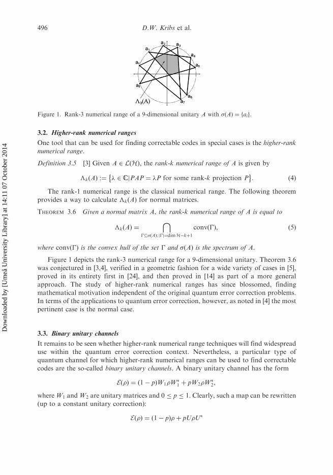
Figure 1 depicts the rank-3 numerical range for a 9-dimensional unitary. Theorem 3.6

was conjectured in [3,4], verified in a geometric fashion for a wide variety of cases in [5],

proved in its entirety first in [24], and then proved in [14] as part of a more general

approach. The study of higher-rank numerical ranges has since blossomed, finding

mathematical motivation independent of the original quantum error correction problems.

In terms of the applications to quantum error correction, however, as noted in [4] the most

pertinent case is the normal case.

3.3. Binary unitary channels

It remains to be seen whether higher-rank numerical range techniques will find widespread

use within the quantum error correction context. Nevertheless, a particular type of

quantum channel for which higher-rank numerical ranges can be used to find correctable

codes are the so-called binary unitary channels. A binary unitary channel has the form

Eð�Þ ¼ ð1� pÞW1�W�1 þ pW2�W

�2,

whereW1 andW2 are unitary matrices and 0 p 1. Clearly, such a map can be rewritten

(up to a constant unitary correction):

Eð�Þ ¼ ð1� pÞ�þ pU�U�

Figure 1. Rank-3 numerical range of a 9-dimensional unitary A with �ðAÞ ¼ faig.


Dow

nloa

ded

by [

Um

eå U

nive

rsity

Lib

rary

] at

14:

11 0

7 O

ctob

er 2

014

where U ¼W�1W2 is again a unitary matrix. The noise operators are therefore A1 ¼ffiffiffiffiffiffiffiffiffiffiffi1� pp

I and A2 ¼ffiffiffipp

U.Theorem 3.4 says that a code C is correctable for E if (3) is satisfied. Given that A�1A1

and A�2A2 are scalar multiples of the identity, two of four requirements are trivially

satisfied. The remaining two requirements both amount to PCUPC ¼ �PC which means

that there is a rank-k correctable code for E if and only if �kðUÞ 6¼ ;. Furthermore, as U

is a normal matrix, we can apply Theorem 3.6.Each � 2 �kðUÞ corresponds to a particular family of codes of dimension k that are

correctable for E. Therefore, in the case of binary unitary channels, we have a robust

method for finding correctable codes of any size for a given channel.

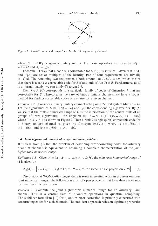
Example 3.7 Consider a binary unitary channel acting on a 2-qubit system (dimH ¼ 4).

Let the eigenvalues of U be �ðUÞ ¼ fuig and f ig the corresponding eigenvectors. By (5)

we see that the rank-2 numerical range of U is the intersection of the convex hulls of all

groups of three eigenvalues – the singleton set � ¼ tu1 þ ð1� tÞu3 ¼ su2 þ ð1� sÞu4� �

where 0 s, t 1 as shown in Figure 2. Then a rank-2 (single qubit) correctable code for

a binary unitary channel is given by C ¼ span j�1iÞ, j�2ið where j�1i ¼ffiffitpj 1iþffiffiffiffiffiffiffiffiffiffi

1� tp

j 3i and j�2i ¼ffiffispj 2i þ

ffiffiffiffiffiffiffiffiffiffiffi1� sp

j 4i.

3.4. Joint higher-rank numerical ranges and open problems

It is clear from (3) that the problem of describing error-correcting codes for arbitrary

quantum channels is equivalent to obtaining a complete characterization of the joint

higher-rank numerical range.

Definition 3.8 Given A ¼ ðA1,A2, . . . ,AdÞ, Ai 2 LðHÞ, the joint rank-k numerical range of

A is given by

�kðAÞ � � ¼ ð�1, . . . , �dÞ 2 CdjPAiP ¼ �iP for some rank-k projection P 8i

n oð6Þ

Discussions at WONRA08 suggest there is some interesting work in progress on these

joint numerical ranges. The following is a list of open problems that have direct relevance

to quantum error correction.

Problem 1 Compute the joint higher-rank numerical range for an arbitrary Pauli

channel. This is a central class of quantum operations in quantum computing.

The stabilizer formalism [10] for quantum error correction is primarily concerned with

constructing codes for such channels. The stabilizer approach relies on algebraic properties

Figure 2. Rank-2 numerical range for a 2-qubit binary unitary channel.


Dow

nloa

ded

by [

Um

eå U

nive

rsity

Lib

rary

] at

14:

11 0

7 O

ctob

er 2

014

of the Pauli group, and hence it would be interesting to compare codes obtained through

a potentially complementary numerical range approach with the stabilizer codes.

Problem 2 Compute the joint higher-rank numerical range for the class of randomized

unitary channels, which are channels with noise operators fAig given by scalar multiples of

unitary operators. Such channels are central in many quantum information investigations,

and include the Pauli channels as a special case. This class is also a natural one to consider

from the mathematical perspective since the higher-rank numerical ranges of unitary

operators are now completely understood.

Problem 3 Compute the joint higher-rank numerical ranges for channels with mutually

commuting normal noise operators fAig. In this case, the spectral theorem gives a joint

eigenspace decomposition for the Ai, which should be useful in code constructions. As

an example that builds on the binary unitary case, one could consider independent and

identically distributed (i.i.d.) noise over a composite quantum system; �E ¼ E � E � � � � � E,

where E has noise operators f 1ffiffi2p I, 1ffiffi

2p Ug.

Problem 4 Stinespring’s dilation theorem gives an important description (1) of

a quantum channel E as a piece of a unitary U acting on a larger Hilbert space. Is it

possible to somehow recognize the quantum error-correcting code structure of E in terms

of properties of U? In particular, do the higher-rank numerical ranges of the unitary U give

information on this code structure?

Problem 5 Formulate the higher-rank numerical range machinery in a continuous time

picture. The characterization (3) of quantum error-correcting codes arises from the

discrete ‘snapshot’ description of open quantum system dynamics, but it would be

interesting to see what higher-rank numerical range differences arise when continuity

enters the picture.

4. Gate fidelities and numerical ranges

Quantum process tomography [17] is the standard method used to fully characterize the

noise affecting experimental implementations of quantum information processing. Often

the desired quantum channel is a unitary transformation, or a unitary ‘gate’, that could be

the mathematical description of a particular quantum algorithm or quantum logic gate for

instance. This ‘target operation’ is implemented by a quantum channel that arises through

the appropriate modulation of a physical Hamiltonian for the system, which we call the

‘physical operation’. Thus, two distinct mathematical and physical perspectives that

generate quantum channels are brought together, with the goal of obtaining channels that

are ‘close’ to each other. Quantum process tomography, and quantum information more

generally, is therefore naturally concerned with the various metrics that can estimate how

close quantum channels are to each other.One possible metric is the fidelity between the states that result from applying the target

and physical operations to identical copies of a particular quantum state j i, where

h j i ¼ 1. For a given target unitary U, the associated channel is denoted by

Uð�Þ ¼ Uð�ÞU�. Letting y denote the dual of a quantum operation, and E denote the

physical operation, the gate fidelity for a state j i is defined as

F ðE,UÞ :¼ h jUy � Eðj ih jÞj i: ð7Þ


Dow

nloa

ded

by [

Um

eå U

nive

rsity

Lib

rary

] at

14:

11 0

7 O

ctob

er 2

014

In the case where the physical operation is also known to be a unitary V – this expression

is greatly simplified to

F ðE,UÞ ¼ jh jU�Vj ij2, ð8Þ

thus demonstrating the connection between gate fidelities and numerical ranges. This is

particularly relevant to the task of designing optimal quantum control sequences.

The evolution of the system under a proposed sequence of control operations can be

simulated on a classical computer and the simulated unitary V can then be compared

to the desired unitary using the fitness function (Equation (8)) (or generalizations below).

The control field can then be numerically optimized to maximize the fitness function [21].

This approach has had success in a variety of implementations of quantum information

processing such as NMR [19], superconducting qubits [22] and ion traps [16].The above two expressions for the gate fidelity are dependent on choice of the state j i.

In order to eliminate this dependency, there are two standard approaches: averaging over

all states uniformly, or choosing the state which minimizes the gate fidelity [9]. In the case

where E has noise operators fAig acting on a Hilbert space of dimension D, this average

gate fidelity Fg is defined as

FgðE,UÞ :¼

Zh jUy � Eðj ih jÞj id ¼

Pi jTrðU

�AiÞj2 þD

D2 þDð9Þ

where the integral is over the Fubini–Study pure state measure [1]. In the case where

physical operation is unitary, this average is the centroid of the numerical range of the

product of the target unitary and the adjoint of the physical unitary. The target and

physical operations are indistinguishable precisely when Fg ¼ 1, and Fg decreases as E acts

on states in a manner more and more different from U. The main disadvantage of this

approach is that it is possible to construct two processes that have a very high average

fidelity, but yet for some input state j i the gate fidelity is zero. In particular, for

dimension D, such a construction can yield Fg 1�Oð1=DÞ while F ¼ 0 for some j i.In order to avoid this problem we consider the worst-case gate fidelity F, which is

defined as

FðE,UÞ ¼ minj i

F ðE,UÞ: ð10Þ

In the case where both the target and physical processes are unitary, computing F simply

corresponds to finding the complex number with smallest norm inside the numerical range

of U�V, which is a straightforward classical calculation given the eigenvalues of U�V.In the case where E is not unitary but some general quantum operation, the

computation of F using numerical ranges is not so straightforward. Decomposing E into

an operator sum results in

FðE,UÞ ¼ minj i

Xi

jh jU�Aij ij2: ð11Þ

Note that noise operators Ai are not normal in general, and so their numerical range is not

as easily computed. Moreover, instead of finding the minimum over the numerical range of

a single operator, one must consider minimization over multiple numerical ranges of non-

normal operators simultaneously. Here joint numerical range techniques could be useful,

for instance see [8,13,18].


Dow

nloa

ded

by [

Um

eå U

nive

rsity

Lib

rary

] at

14:

11 0

7 O

ctob

er 2

014

A different approach would be to consider a different representation for the

quantum operations and the quantum states. This representation is known as the

Liouville representation [2], where a quantum operation E with noise operators fAig

is represented by

E ¼Xi

A�i � Ai ð12Þ

and a density operator � corresponding to a state is represented by

j�ii ¼ ð11� �ÞXDj¼1

jjijji: ð13Þ

In this representation, Eð�Þ is given by the product Ej�ii, and thus the gate fidelity for

a pure input state � is

hh�jU�Ej�ii ð14Þ

under the constraints that

hh�j�ii ¼ Tr�2 ¼ 1, ð15Þ

hhj�ii ¼ Tr� ¼ 1, ð16Þ

� � 0: ð17Þ

In general, nothing can be said about the diagonalizability of E. However, because we

know the gate fidelity for valid states is always non-negative and at most 1, we canconsider the numerical range for only the Hermitian part of U�E. What remains unclear is

how to enforce the constraints that hh11j�ii ¼ 1 and � � 0, which are necessary in order to

ensure that the input state be a valid pure quantum state. Although this minimization can

be performed numerically [9], the problem of analytically solving for the worst-case gatefidelity between a unitary and a general quantum operation remains open.

In some experimentally relevant cases, some restrictions may be placed on E. For

particular systems, the non-unitary evolution comes from inhomogeneities in either

time or space. The leads to a channel which is a generalization of the binary unitarychannel to a distribution over unitaries. Solving the worst case fidelity in this restricted

case might be a useful first step – as would solving it in any of the special cases

outlined in the problems posed in the previous section. We state this as a single meta

problem.

Problem 6 Find a technique to analytically compute the worst-case gate fidelity (11)

between a unitary and a general quantum operation (CPTP map).

Acknowledgements

D.W. Kribs is grateful for several interesting conversations with participants of WONRA08, andfor helpful conversations with M.B. Ruskai. D.W. Kribs was partially supported by NSERCgrant 400160, by NSERC Discovery Accelerator Supplement 400233, and by Ontario EarlyResearcher Award 048142. A. Pasieka was partially supported by an Ontario Graduate Scholarship.


Dow

nloa

ded

by [

Um

eå U

nive

rsity

Lib

rary

] at

14:

11 0

7 O

ctob

er 2

014

M.P. da Silva and C. Ryan were partially supported by NSERC, M. Laforest was partiallysupported by NSERC and FQRNT.

References

[1] I. Bengtsson and K. _Zyczkowski, Geometry of Quantum States: An Introduction to Quantum

Entanglement, Cambridge University Press, Cambridge, UK, 2006.[2] K. Blum, Density Matrix Theory and Applications, Springer, New York, 1996.

[3] M.D. Choi, D. Kribs, and K. _Zyczkowski, Higher-rank numerical ranges and compression

problems, Lin. Alg. Appl. 418 (2006), pp. 828–839.[4] M.D. Choi, D.W. Kribs, and K. _Zyczkowski, Quantum error correcting codes from the

compression formalism, Rep. Math. Phys. 58 (2006), pp. 77–91.[5] M.D. Choi, J. Holbrook, D. Kribs, and K. _Zyczkowski, Higher-rank numerical ranges of unitary

and normal matrices, Oper. Matrices 1 (2007), pp. 409–426.[6] G. Dirr, U. Helmke, M. Kleinsteuber, and T. Schulte-Herbruggen, Relative C-numerical ranges

for applications in quantum control and quantum information, Lin. Multilin. Alg. 56 (2008),

pp. 27–51.[7] L.M. Duan and G.C. Guo, Preserving coherence in quantum computation by pairing quantum

bits, Phys. Rev. Lett. 79 (1997), pp. 1953–1956.[8] M.K.H. Fan and A.L. Tits, m-Form numerical range and the computation of the structured

singular value, IEEE Trans. Automat. Contr. 33(3) (1988), pp. 284–289.

[9] A. Gilchrist, N.K. Langford, and M.A. Nielsen, Distance measures to compare real and ideal

quantum processes, Phys. Rev. A 71 (2005), pp. 062310–062324.[10] D. Gottesman, Class of quantum error-correcting codes saturating the quantum Hamming bound,

Phys. Rev. A 54 (1996), pp. 1862–1883.[11] E. Knill and R. Laflamme, Theory of quantum error-correcting codes, Phys. Rev. A 55 (1997),

pp. 900–905.[12] E. Knill, R. Laflamme, and L. Viola, Theory of quantum error correction for general noise,

Phys. Rev. Lett. 84 (2000), pp. 2525–2528.

[13] C.K. Li and Y.T. Poon, Convexity of the joint numerical range, SIAM J. Matrix Anal. Appl. 21

(1999), pp. 668–678.[14] C.K. Li and N.S. Sze, Canonical forms, higher rank numerical ranges, totally isotropic subspaces,

and matrix equations, Proc. Amer. Math. Soc. 136 (2008), pp. 3013–3023.[15] D. Lidar, I. Chuang, and K. Whaley, Decoherence-free subspaces for quantum computation,

Phys. Rev. Lett. 81 (1998), pp. 2594–2597.

[16] V. Nebendahl, H. Haffner, and C.F. Roos, Optimal control of entangling operations

for trapped ion quantum computing, preprint. Available at arXiv:0809.1414 (2008).

[17] M.A. Nielsen and I.L. Chuang, Quantum Computation and Quantum Information, Cambridge

University Press, New York, 2000.[18] Y.T. Poon, On the convex hull of the multiform numerical range, Lin. Multilin. Alg. 37 (1994),

pp. 221–223.[19] C.A. Ryan, C. Negrevergne, M. Laforest, E. Knill, and R. Laflamme, Liquid-state nuclear

magnetic resonance as a testbed for developing quantum control methods, Phys. Rev. A 78 (2008),

pp. 012328–012342.[20] T. Schulte-Herbruggen, A. Sporl, N. Khaneja, and S.J. Glaser, Optimal control-based efficient

synthesis of building blocks of quantum algorithms: A perspective from network complexity

towards time complexity, Phys. Rev. A. 72 (2005), pp. 042331–042337.[21] T. Schulte-Herbruggen, A. Sporl, N. Khaneja, and S.J. Glaser, Optimal control for generating

quantum gates in open dissipative systems, preprint. Available at arXiv:quant-ph/0609037v1

(2006).


Dow

nloa

ded

by [

Um

eå U

nive

rsity

Lib

rary

] at

14:

11 0

7 O

ctob

er 2

014

[22] A. Sporl, T. Schulte-Herbruggen, S.J. Glaser, V. Bergholm, M.J. Storcz, J. Ferber, andF.K. Wilhelm, Optimal control of coupled Josephson qubits, Phys. Rev. A 75 (2007),pp. 012302–012309.

[23] W. Stinespring, Positive functions on C*-algebras, Proc. Amer. Math. Soc. 6 (1955), pp. 211–216.

[24] H.J. Woerdeman, The higher rank numerical range is convex, Lin. Multilin. Alg. 56 (2008),pp. 65–67.

[25] P. Zanardi, Stabilizing quantum information, Phys. Rev. A 63 (2001), pp. 12301–12305.

[26] P. Zanardi and M. Rasetti, Noiseless quantum codes, Phys. Rev. Lett. 79 (1997), pp. 3306–3309.


Dow

nloa

ded

by [

Um

eå U

nive

rsity

Lib

rary

] at

14:

11 0

7 O

ctob

er 2

014

Documents

Research problems on numerical ranges in quantum computing