Embed Size (px)
Citation preview
research paper series Theory and Methods
Research Paper 2008/36
Endowment Differences and the Composition of Intra-Industry Trade
by
Manuel Cabral, Rod Falvey and Chris Milner
The Centre acknowledges financial support from The Leverhulme Trust under Programme Grant F/00 114/AM
The Authors Manuel Cabral is a Professor Auxiliar at the University of Minho, Rod Falvey is Professor of
International Economics and Research Fellow in GEP and Chris Milner is Professor of
International Economics and Research Fellow in GEP.
Acknowledgements Falvey and Milner gratefully acknowledge financial support from the Leverhulme Trust under Programme Grant F/00 114/AM. All the authors are grateful for helpful comments on earlier drafts of the paper provided by Rob Elliott, Paulo Bastos, Joanna Silva and Paula Veiga.
Endowment Differences and the Composition of Intra-Industry Trade
by
Manuel Cabral, Rod Falvey and Chris Milner
Abstract This paper investigates the relationship between differences in endowments and different types of trade, in particular vertical intra-industry trade (VIIT). We build a general equilibrium framework based on a hybrid of the Chamberlain-Heckscher-Ohlin and the specific factors models that generates predictions about how the shares of different types of intra-industry and net trade flows change with differences in endowments. We also present some empirical evidence for European Union trade with its 51 major trading partners. The econometric models of the determinants of the different types of trade confirm the theoretical predictions, namely that the effect of cross country differences in the endowments of trading partners on the share of vertical IIT in total bilateral trade differs from their effect on both horizontal IIT and net trade. The share of horizontal IIT (net trade) decreases (increases) for all increases in absolute endowment differences, but the share of vertical IIT can both increase and decrease with increases in endowment differences.
JEL classification: F11, F14
Keywords: Intra-industry trade, factor endowments
Outline
1. Introduction
2. Relationship to the existing empirical literature
3. Some evidence on endowment differences and trade patterns 3
4. A general equilibrium framework..
5. Empirical modelling and strategy
6. Regression results
7. Conclusions
Non-Technical Summary
Factor endowment differences play an important role in international trade theory, for both the pattern and volume of trade. Both the Heckscher-Ohlin and monopolistic competition models predict that the share of net or inter-industry trade in total trade will be larger the greater the differences in relative factor endowments between countries. Monopolistic competition models also involve intra-industry trade (IIT), which is generally assumed to be horizontal (HIIT) in nature, involving the exchange of differentiated varieties of the same good, produced using a common increasing returns to scale technology, and therefore involving no net exchange of factor services. This can be distinguished from matched exchanges of vertically differentiated commodities - vertical intra-industry trade (VIIT) - which involves the exchange of different qualities of the same good, produced using different technologies. Explanations of VIIT involve differences in endowments (between countries) and in factor requirements within each industry.
While theory has focused on HIIT, empirical studies reveal that VIIT is the dominant type of trade for most developed countries, and that VIIT embodies net exchanges of factor services. The presumption has been that VIIT, like net trade (NT), will show a positive monotonic relationship with endowment differences between countries. But existing trade models do not allow us to draw clear inferences about this, and we show that the data suggests a more complex relationship between VIIT and differences in endowments. In order to clarify both the relationship between VIIT and HIIT and that between VIIT and NT, we develop a framework that allows for the simultaneous existence of HIIT, VIIT and NT, from which we are able to draw some testable hypotheses about the relation between endowment differences and the shares of HIIT, VIIT and NT in total bilateral trade. The predictions for HIIT are quite conventional - larger endowment differences would reduce such trade. But the predictions for VIIT are more factor and trading partner specific. VIIT should grow with differences in sector specific factor endowments, as long as these differences remain small. The effects of larger specific factor endowment differences depend on whether the specific factor is used by the industry. If not, then VIIT declines for larger endowment differences. If so, then the share of VIIT increases (decreases) if the trading partner has an ever larger (smaller) endowment.
We test these hypotheses for European Union trade with its 51 major trading partners. Our results confirm that HIIT declines with growing endowment differences. They also confirmed the sensitivity of VIIT flows to the magnitude of endowment differences. The specific predictions on endowment differences in the specific factor used by the industry (assumed to be capital) are also confirmed. But the nonlinearities predicted for the other specific factor (assumed to be land) do not appear, perhaps due to insufficient variability in the sample. Overall these findings support the view that both within and between industry specialization and trade can be driven by factor endowment considerations, and undermine the view that VIIT is simply disguised inter-trade associated with industry (mis)aggregation.
1. Introduction
Differences in endowments play a central role in international trade theory. According to both
the Heckscher-Ohlin and the monopolistic competition models (Helpman 1981, Helpman and
Krugman 1995), the share of net or inter-industry trade in total trade is expected to be larger the
greater the differences in relative factor endowments between countries. Monopolistic
competition models also involve intra-industry trade (IIT), which is generally assumed to be
horizontal (HIIT) in nature – i.e. to involve the exchange of differentiated varieties of the same
good, produced using a common increasing returns to scale technology – and therefore to
involve no net exchange of factor services. This can be distinguished from matched exchanges
of vertically differentiated commodities - vertical intra-industry trade (VIIT) - which involves
the exchange of different qualities of the same good, produced using different technologies.
Explanations of VIIT involve differences in endowments (between countries) and in factor
requirements within each industry (e.g. Falvey, 1981; Falvey and Kierzkowski, 1987; and
Gullstrand, 2000).
While most of the theory has focussed on HIIT, empirical studies reveal that matched exchanges
of vertically differentiated commodities are the dominant type of trade in most developed
countries1 2, and that VIIT embodies net exchanges of factor services . These studies have tended
to presume that, like net trade (NT), there is a positive monotonic relationship between the
extent of endowment differences between countries and the share of VIIT in total bilateral trade.
But existing trade models do not allow us to draw clear inferences about this, and we show
below that the data suggest a more complex relationship between VIIT and differences in
endowments.
Responding to this evidence and to the need to clarify both the relationship between VIIT and
HIIT and that between VIIT and net trade, we develop a framework that links the Chamberlain-
Heckscher-Ohlin (C-H-O) model with the specific factors model. In doing this we follow a
similar line to Krueger (1977) and Deardorff (1984), who combine elements from the
Heckscher-Ohlin and specific factor models3. The result is a modelling framework that allows
for the simultaneous existence of HIIT, VIIT and NT, from which we are able to draw some 1 E.g. Greenaway et al. (1994, 1995), Durkin and Krygier (2000), Blanes and Martin (2000) and Fukao et al. (2003). 2 Using factor content analysis, Cabral, Falvey and Milner (2005) show that the net exchanges of factors embodied in VIIT are as intense as those embodied in the same volume of net trade and are consistent with the factor abundance predicted by the endowments.
1
testable hypotheses about the relation between endowment differences and the shares of HIIT,
VIIT and NT in total bilateral trade. In particular, we argue that the relation between VIIT and
inter-country endowment differences is not necessarily monotonic, with the share of VIIT
increasing with small differences in endowments but decreasing for wider differences in
endowments. To test these hypotheses we follow the method used by Greenaway et al. (1994;
1995), disentangling VIIT from HIIT, and estimating separate regressions for the determinants
of each of these types of trade flows. We also follow the suggestion of Hummels and Levinsohn
(1995) and use direct measures of the endowments as country determinants.
The remainder of the paper is organised as follows. Section 2 presents the relationship of the
present work with the existing empirical literature. Section 3 presents some descriptive evidence
on the patterns of EU trade and endowment differences with its trading partners. Section 4 sets
up the model and extracts the hypotheses to be tested empirically. Section 5 outlines our
empirical strategy and section 6 presents the results of the econometric testing. The conclusions
of the study are set out in section 7.
2. Relationship to the Existing Empirical Literature Early empirical studies of the determinants of IIT tended to test the C-H-O model of IIT on the
presumption that IIT was predominantly two-way trade in horizontally differentiated goods
which did not involve significant net exchanges of factor services. This was consistent with the
evidence that IIT dominated North-North trade, while net trade or inter-industry trade which did
embody important exchanges of factor services dominated North-South trade. Using total IIT
most of these studies found negative signs for the difference in GDP per capita variable (used as
a proxy for differences in endowments), which was seen as confirmation of the C-H-O model.
But Hummels and Lehvison (1995) cast doubt on the robustness of these results. Using direct
measures of endowments (rather than GDP per capita) they obtain results contrary to the C-H-O
predictions. One explanatory factor is that the early empirical work on the determinants of IIT
did not separate vertical from horizontal matched exchanges, and more recent work reveals that
matched trade flows may include net exchanges of factor services similar to those included in
net trade, when these consist of exchanges of vertically differentiated commodities (Cabral,
Falvey and Milner, 2006).
3 In a similar fashion Davis (1995) adds Ricardian elements (technology differences) to the HO model to explain HIIT under constant returns to scale technologies and perfectly competitive markets.
2
The work of Abd-el-Raman (1991) and Greenaway et al. (1994) established a method to
separate vertical from horizontal IIT, and provided evidence that matched exchanges of
vertically differentiated commodities are the dominant form of IIT, even in the trade between
developed countries4. Most of the studies that disentangle vertical from horizontal IIT
hypothesize a positive relationship between endowment differences and VIIT and a negative
relationship between HIIT and endowment differences. The studies that run separate regressions
for horizontal and vertical IIT failed to confirm these expectations for VIIT. Rather they reveal
contradictory results. Greenaway et al. (1994, 1999)5, Blanes and Martin (2000) and Fukao et al.
(2003) obtained negative signs for the differences in GDP per capita when used to explain VIIT,
while Gullstrand (1999), Martin-Montaner and Orts Rios (2002), Durkin and Krygier (2000),
and Crespo and Fontoura (2001) found positive signs on the same variable. The use of direct
measures of factors, as suggested by Hummels and Levinsohn (1995), has been applied in only a
few of the empirical studies that separate vertical from horizontal IIT. Martin-Montaner and
Orts Rios (2002) found a positive and significant relationship between VIIT and differences in
endowments of human capital and capital per worker6. Crespo and Fontoura (2001) find,
however, a negative sign for the case of differences in human capital7.
Here we argue that the approach followed by the earlier empirical studies was mistaken in
expecting VIIT to behave like HIIT. We also argue that the hypothesis considered in recent
empirical studies, namely that the share of VIIT flows in total trade is related to differences in
endowments in the same way as NT, cannot necessarily be inferred from a general equilibrium
framework that allows for simultaneous HIIT, VIIT and NT flows and is not reflected in the
data.
4The Greenaway et al. (1994) study of the UK trade in 1988 report that about 70% of the matched trade should be classified as vertical intra-industry trade. Similar evidence was presented by Abd-el Raman (1991), for French trade in 1985-87, and by Durkin and Krygier (1997) for US trade with the OECD countries in 1989 to 1992. In our calculations we found that VIIT accounts for 78% of the bilateral IIT between the UK and the OECD countries in 1996. 5The Greenaway et al. (1994) results show a negative sign for the variable differences in GDP per capita both for vertical and horizontal IIT. Greenaway et al. (1999) also found negative signs for differences in per capita income, but obtained a positive sign for differences in the capital stock per worker. This corresponded to what they expected for VIIT, but not for HIIT, for which the same sign is reported. 6 Note that their study is concerned only with the trade of Spain with the OECD countries. Most of these countries have higher GDP per capita than Spain. This may influence their result, which is interesting and valid but probably refers only to one type and not to the whole of VIIT flows. See section 6. 7 Fukao et al. (2003) also consider differences in human capital, but obtain insignificant results.
3
3. Some Evidence on Endowment Differences and Trade Patterns We follow Abd-el-Rahman (1991) and Greenaway et al. (1994) and use the unit values of
exports and imports to determine if matched exchanges of a particular sector are considered as
VIIT or HIIT. For each product the ratio Xij ijUV UV M , where and are the unit value
of exports and imports (the price per tonne) of the sub-sector j which is included in industry i,
determines the quality of the exports relative to the imports. For values of this ratio in the
interval:
XijUV M
ijUV
αα +≤≤− 11 Mij
Xij
UVUV
the matched trade of the sub-sector i is considered as HIIT, while for values below or above it is
considered VIIT8. The Grubel and Lloyd (GL) index of IIT for each type of trade flow is given
by:
∑∑∑+
−−+=
iicic
iicic
iicic
MX
MXMXGL
)(
||)(* **
****
where the X* and M* represent the exports and imports of each commodity that are considered
to be of type * (i.e. are considered to be horizontally or vertically differentiated).
Applying this methodology to the EU member countries’ trade with 51 major trading partners in
2002, Figure 1(a) shows an inverse relationship between VIIT and differences in GDP per
worker overall, although with some tendency for the share of VIIT to rise for small endowment
differences9. This is certainly not in line with the traditional expectation of a positive
relationship. VIIT tends, however, to be higher the more developed (level of GDP per worker) is
the partner country of the EU (see Figure 1(b)). This does correspond with other findings that
VIIT is predominantly North-North in nature.10 Figures 1(c) and 1(d) show the relation between
differences in GDP per worker and HIIT and NT. The clear picture that emerges is that the share
of HIIT decreases with differences in GDP per worker and that of NT increases with endowment
differences, as the CHO model predicts. Also, when one plots the level of GDP per worker (or 8 When the price per unit (tonne) of the exports exceeds that of the imports by a significant margin the proportion given by the parameter (α) will determine that VIIT is high quality, when it is below the interval that the vertical IIT is low quality. There is a degree of arbitrariness in the selection of the dispersion criterion which may give rise to concerns (see for example Nielsen and Luthje, 2002). The methodology does allow a comprehensive measurement of trade types, however. 9 Graphics for GDP per capita and capital per worker were also calculated. The plotted results are very similar for the relation of the share of VIIT in total trade with each of these three variables (GDP per worker, GDP per capita or Capital per worker).
4
per capita) the proportion of NT in total trade tends to be smaller the larger is GDP per worker,
while the proportion of HIIT tends to be larger the larger is the GDP per worker of the trading
partner of the EU. This corresponds well with the established idea that (HIIT) takes place in
North-North trade, while inter-industry trade dominates North-South trade.
It is evident from these Figures that VIIT is different to both HIIT and NT in terms of its
relationship to endowment differences for this sample of countries. This is even clearer when we
separate the countries in our sample into high income countries (Figure 1(e)) and middle and
low income countries (Figure 1(f))11. The first group includes countries with similar or higher
per capita incomes than the EU average, while the second group includes countries that are all
below the EU average. The plots indicate a positive relationship between VIIT and differences
in endowments for the first group of countries, and a negative relationship for the latter. For
large samples of countries, including those with both larger and smaller endowments, we should
not therefore expect to generate a monotonic relationship between differences in endowments
and VIIT.
If one separates the countries so that only countries above (below) the average are included, the
results expressed in differences became very similar to those expressed in levels, since the larger
(smaller) the GDP per worker (or per capita) the larger will be the difference in GDP per
worker. When we are dealing only with countries with a higher (lower) level of development
most of the VIIT will be of the type where the reference country exports (imports) the lower
quality varieties and imports (exports) the higher quality. In such samples one is studying only
one type of vertical IIT and its relation with the level of endowments or income per capita. In
this sense, the evidence obtained in those studies (e.g. Martin-Montaner and Orts Rios, 2002;
Gabrisch and Segana, 2002), should be seen as modelling of the determinants of a type of VIIT,
not of VIIT in general.
10 Although it is worth noting that the share of VIIT is much larger in the trade between the EU and less developed countries in particular. 11 Countries with more than $US 20,000 of per capita income in 2002 were considered to be High Income and include Australia, Austria, Belgium, Canada, Denmark, Finland, France, Germany, Hong Kong, Ireland, Italy, Japan, Netherlands, New Zealand, Norway, Singapore, Sweden, Switzerland, UK, USA. Those with income per capita less than $US 20,000 were included in Middle Income and Developing – namely Argentina, Brazil, Bulgaria, Chile, China, Colombia, Costa Rica, Croatia, Czech Rep., Estonia, Greece, Hungary, India, Indonesia, Israel, Malaysia, Mexico, Peru, Philippines, Poland, Portugal, Romania, Russia, Slovakia, Slovenia, South Africa, South Korea, Spain. Sri Lanka, Thailand, Turkey, Venezuela.
5
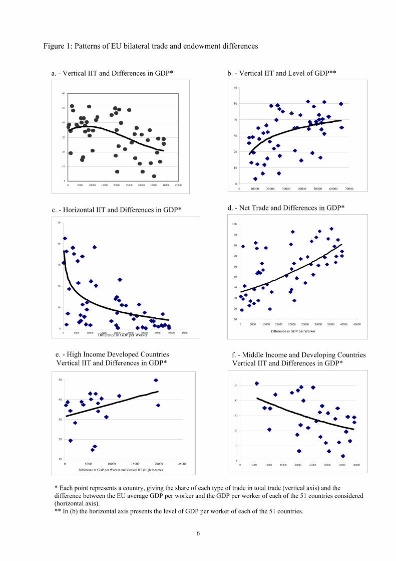
Figure 1: Patterns of EU bilateral trade and endowment differences
a. - Vertical IIT and Differences in GDP*
0
10
20
30
40
50
60
0 5000 10000 15000 20000 25000 30000 35000 40000 45000
c. - Horizontal IIT and Differences in GDP*
0
10
20
30
40
50
0 5000 10000 15000 20000 25000 30000 35000 40000 45000Difference in GDP per Worker
e. - High Income Developed Countries
Vertical IIT and Differences in GDP*
10
20
30
40
50
0 5000 10000 15000 20000 25000
Difference in GDP per Worker and Vertical IIT (High Income)
b. - Vertical IIT and Level of GDP**
0
10
20
30
40
50
60
0 10000 20000 30000 40000 50000 60000 70000
d. - Net Trade and Differences in GDP*
10
20
30
40
50
60
70
80
90
100
0 5000 10000 15000 20000 25000 30000 35000 40000 45000
Difference in GDP per Worker
f. - Middle Income and Developing Countries Vertical IIT and Differences in GDP*
0
10
20
30
40
50
0 5000 10000 15000 20000 25000 30000 35000 40000
* Each point represents a country, giving the share of each type of trade in total trade (vertical axis) and the difference between the EU average GDP per worker and the GDP per worker of each of the 51 countries considered (horizontal axis). ** In (b) the horizontal axis presents the level of GDP per worker of each of the 51 countries.
6
4. A General Equilibrium Framework In this section we lay out a simple general equilibrium model that features the simultaneous
presence of HIIT, VIIT and NT, in order to illustrate their interactions and to explore their links
with factor endowments. We do this by combining models that are familiar from the literature -
the CHO model (Helpman, 1981; Helpman and Krugman, 1985), which explains HIIT and NT
in a general equilibrium setting; the partial equilibrium VIIT model (Falvey, 1981); and a hybrid
Heckscher-Ohlin-Specific-Factors model introduced by Krueger (1977) and developed by
Deardorff (1984). In short, we model HIIT as the exchange of high quality, capital-intensive,
differentiated products in a monopolistically competitive market; VIIT as the exchange of these
products for a basic lower quality, labour-intensive, homogeneous manufactured product; and
NT as the exchange of either of these products for a homogeneous agricultural output which is
produced using land and labour.
Assumptions
We consider two sectors. Agriculture employs land and labour to produce a homogeneous
product (denoted by A) using a constant returns to scale technology. Manufacturing uses capital
and labour, and produces two types of output, a homogeneous, basic product (denoted by B),
and differentiated higher quality varieties (denoted by D)12. The basic product is produced under
a constant returns to scale technology by competitive firms. Production of the differentiated
varieties is best viewed as taking place in two steps. First, capital and labour are combined to
produce a (hypothetical) homogeneous input (denoted by I) using a constant returns to scale
technology that is more capital intensive than that used in the basic output. This input is then be
used to produce the differentiated varieties, via a standard Krugman (1979) technology where
production of each variety involves a fixed cost and a constant marginal cost, both expressed in
terms of the hypothetical input. This leads to each variety being produced by a single firm in a
monopolistically competitive setting. For convenience, units of differentiated output are chosen
so that the marginal cost of producing one unit of differentiated output is one unit of the
hypothetical input. Thus production of x units of a differentiated variety requires
Ix f x= +
units of hypothetical input, where denotes the fixed cost. 0f >
12 The underlying idea is that in manufacturing industries a relatively small number of large firms compete with a fringe of a large number of small firms. The former in many cases are companies that produce differentiated goods
7
All goods are traded internationally, and all countries have access to the same production
technologies13. As in most trade models, preferences are assumed to be identical across
countries. We follow Krugman (1979) in assuming that there is love for variety in the demand
for the differentiated varieties. We further suppose that the utility of the representative consumer
is a Cobb-Douglas function of consumption of the agricultural good, the basic manufactured
product and a composite of the differentiated varieties:
A B DU c c uα β δ=
1
1
n
D jj
u cρ
ρ
=
⎡ ⎤= ⎢ ⎥⎣ ⎦∑where , 0 1ρ< < is the differentiated variety composite. Profit maximisation
implies that the price of a typical variety ( Dp ) is a markup on its marginal cost
1D Ip pεε
=−
Ipwhere is the cost of a unit of the hypothetical input. Free entry implies zero profits in
equilibrium, which leads to an optimum firm size of
[ 1x f ]ε= −
Since preferences are identical and symmetric, and the same amount of each variety is produced
in equilibrium, their prices must be identical. This implies, given a common markup, that the
unit price of the hypothetical input must also be identical across countries. Trade will equalize
the prices of the basic manufactured output and the agricultural good (which will be taken as the
numeraire). A country producing all three types of output in equilibrium will have competitive
profit conditions
( )1 ( ,A A )p c w v≡ =
( , )B Bp c w r=
( , )I Ip c w r=
where is the unit cost function for output , ,j A B I=(.,.)jc , which depend only on factor prices
since their respective technologies are all CRS. Two countries that produce all three outputs will
(with strong brand identification) under increasing returns to scale, while the latter are small firms that compete on a cost basis. 13 As noted earlier, Davis (1995) explains IIT by extending the HO model to include cross-country technology differences in the different goods produced by a multi-product industry. His objective is to explain IIT in goods produced with similar factor intensities, and thus involving negligible net embodied-factor trade, which are the characteristics of HIIT. Since the evidence suggests that VIIT does involve net embodied-factor trade, an assumption of technology differences across goods of differing quality seems appropriate here.
8
have the same factor prices and therefore, given common technologies, produce using the same
input combinations. Their mix of outputs will depend on their factor endowments, however.
Diagrammatic representation
The patterns of specialization and trade in this model can be represented using the technique
employed by Deardorff (1984, p.735). The upper panel in Figure 2 represents the tangency of a
unit cost line (whose slope represents the relative costs of capital and labour in the non-
specialised equilibrium) with the unit value isoquants for the two manufacturing outputs (B and
I). This tangency determines the equilibrium capital-labour ratios employed in this industry
when both outputs are produced ( ). Suppose the country’s capital stock is given by .
Then its equilibrium output mix in the manufacturing sector depends on that sector’s
employment of labour. If this is less than
,I Bk k EK
1ML , then full employment requires that this country’s
manufacturing specialises in the differentiated varieties, with the capital labour ratio employed
in producing the hypothetical input exceeding , and the factor returns corresponding to their
value marginal products in hypothetical input production. Similarly, if the labour employment in
manufacturing exceeds
Ik
2ML , the sector specialises in the base product which is produced using a
capital labour ratio less than . In between both manufacturing outputs are produced, and
increased employment is absorbed by readjustments of the output mix towards the more labour
intensive basic product at constant factor prices.
Bk
The lower panel in Figure 2 represents the labour market equilibrium diagram familiar from the
specific factors model. The value of the marginal product of labour in the Agricultural sector
depends on the land endowment and the quantity of labour employed in Agriculture, as shown
by the schedule measured relative to the right-hand axis. The corresponding schedule for
manufacturing (
AW
MW ) is downward sloping in the employment ranges where the sector is
specialised in one of the two products, but is horizontal (at the FPE wage rate) in the range
where this sector is non-specialised. The manufacturing employments over which this horizontal
section occurs clearly depend on the size of the capital endowment.
Our objective is to explore how the different factor endowments of countries are reflected in
their trade patterns in this equilibrium. For purposes of comparison we begin with a “reference”
country that is non-specialised in the trading equilibrium and has labour market equilibrium as
9
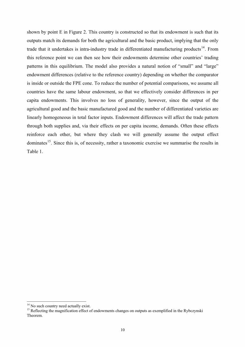
shown by point E in Figure 2. This country is constructed so that its endowment is such that its
outputs match its demands for both the agricultural and the basic product, implying that the only
trade that it undertakes is intra-industry trade in differentiated manufacturing products14. From
this reference point we can then see how their endowments determine other countries’ trading
patterns in this equilibrium. The model also provides a natural notion of “small” and “large”
endowment differences (relative to the reference country) depending on whether the comparator
is inside or outside the FPE cone. To reduce the number of potential comparisons, we assume all
countries have the same labour endowment, so that we effectively consider differences in per
capita endowments. This involves no loss of generality, however, since the output of the
agricultural good and the basic manufactured good and the number of differentiated varieties are
linearly homogeneous in total factor inputs. Endowment differences will affect the trade pattern
through both supplies and, via their effects on per capita income, demands. Often these effects
reinforce each other, but where they clash we will generally assume the output effect
dominates15. Since this is, of necessity, rather a taxonomic exercise we summarise the results in
Table 1.
14 No such country need actually exist. 15 Reflecting the magnification effect of endowments changes on outputs as exemplified in the Rybczynski Theorem.
10
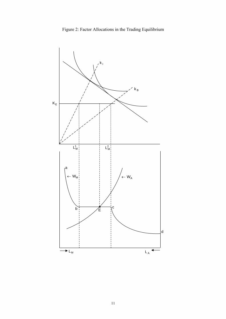
Figure 2: Factor Allocations in the Trading Equilibrium
Bk
Ik
EK
2ML 1
ML
MW
← AW←
b c
a
E
d
ML AL
11
Differences in land endowments
Trade patterns: We begin by considering countries that differ from the reference country only in
their land endowments. A slightly smaller land endowment would leave the intersection between
the two “wage schedules” somewhere in the range Ec. Output of the agricultural good would be
lower and it will be imported. Output of differentiated products (specifically the number of
differentiated products produced) will also be lower, while output of the basic manufactured
good will be higher. This suggests exports of the basic manufactured good in exchange for
imports of differentiated manufactured products and agricultural output. A significantly smaller
land endowment would mean an equilibrium on the cd section of the manufacturing wage
schedule. Such a country would only produce agricultural and basic manufactured products, but
with basic manufactured output much higher and agricultural output much lower than in the
reference country. The former will be imported and the latter exported as a consequence.
Alternatively, a country with a land endowment slightly larger than that of the reference country
(and therefore on Eb), will produce more agricultural goods and differentiated varieties and less
of the basic manufactured product. Its trade pattern will show exports of agriculture and
differentiated varieties, and imports of the basic manufactured product. For a relatively land
abundant country, the labour market equilibrium will lie on section ab of the manufacturing
wage schedule. Production is specialized in differentiated varieties and agricultural goods, but
output of the former is lower than at point b (where output of differentiated varieties is greatest).
The trade pattern involves imports of basic manufactures and exports of the agricultural product
and differentiated varieties, with the latter declining as the land endowment gets larger.
Trade Shares: In this setting there will exist some HIIT between any two countries, as long as
there is some production of the differentiated varieties in both. The share of HIIT is maximized
in the reference country, however, where all trade is HIIT. Since endowment differences
generate other forms of trade, the share of HIIT must fall. A larger land endowment implies: (a)
increased agricultural exports and hence an increased share of NT; and (b) increased imports of
basic manufactures which will involve increased VIIT until production of the differentiated
varieties begins to fall, when VIIT will also begin to decline. A smaller land endowment implies
(a) increased agricultural imports and hence an increased share of NT; and (b) increased exports
of basic manufactures and increased imports of differentiated varieties implying increased VIIT.
But once production of differentiated varieties ceases, there is no HIIT, and imports of
differentiated varieties begin to fall as per capita income declines, implying reduced VIIT.
12
Differences in capital endowments
Trade Pattern: A larger (smaller) capital endowment shifts the downward sloping sections of the
manufacturing wage schedule to the right (left), with a corresponding shift of the horizontal
segment (at the same wage level). A slightly larger (smaller) capital stock than the reference
country (with the same land and labour endowment), leads to no change in agricultural output,
as long as the equilibrium remains on the horizontal section of the manufacturing wage
schedule, and a switch in the composition of manufactured output away from basic
(differentiated) towards differentiated (basic) products. There are net imports (exports) of
agricultural goods because per capita income has risen (fallen), supplemented by the export
(import) of high quality differentiated varieties in exchange for basic product imports (exports).
Larger differences in capital endowments shift the labour market equilibrium to one of the
downward sections of the manufacturing wage schedule. Thus if a country has a much larger
capital endowment than the reference country, its manufacturing sector will specialize in
differentiated varieties, and its output of agricultural goods will be less than the reference. All
basic manufactures consumed are imported, as are some agricultural products. Differentiated
varieties are exported. Alternatively, if a country’s capital endowment is much smaller than that
of the reference country, its manufacturing sector will specialize in the basic product. Its
agricultural output will be higher than in the reference country and its demand (per capita) will
be smaller since its income per capita has fallen. The trading outcome is the export of
agricultural output and basic manufactures for differentiated manufactured imports.
Trade Shares: The share of HIIT falls relative to the reference country for the same reason as
above. An increasing capital endowment leads to (a) increasing agricultural imports and hence
growing NT; and (b) increasing exports of differentiated varieties and imports of basic
manufactures, hence increasing VIIT. All basic manufactures consumed are imported once the
equilibrium is on the (transposed) ab range of the manufacturing wage schedule. A falling
capital endowment leads to (a) increasing agricultural exports implying growing NT; and (b)
increasing exports of basic products in exchange for differentiated varieties, implying increased
VIIT. However, once the capital endowment difference is sufficiently large, production of
differentiated varieties ceases and there is no HIIT. Further decreases in the capital endowment
reduce basic manufactures output and VIIT begins to decline.
13
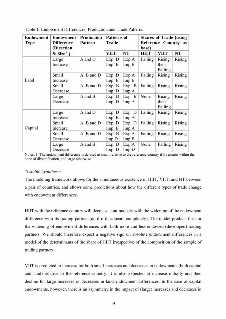
Table 1: Endowment Differences, Production and Trade Patterns
Patterns of Trade
Shares of Trade (using Reference Country as base)
Endowment Endowment ProductionType Difference Pattern
(Direction & Size 1 ) VIIT NT HIIT VIIT NT Large Increase
A and D
Exp D Imp B
Exp A Imp B
Falling Rising then Falling
Rising
Small Increase
A, B and D Exp D Imp B
Exp A Imp B
Falling Rising
Rising
Small Decrease
A, B and D Exp B Imp D
Exp B Imp A
Falling Rising
Rising
Land
Large Decrease
A and B Exp B Imp D
Exp B Imp A
None Rising Rising then
Falling Large Increase
A and D
Exp D Imp B
Exp D Imp A
Falling Rising
Rising
Small Increase
A, B and D Exp D Imp B
Exp D Imp A
Falling Rising
Rising
Small Decrease
A, B and D Exp B Imp D
Exp A Imp B
Falling Rising
Rising
Capital
Large Decrease
A and B Exp B Imp D
Exp A None Falling Rising Imp D
Notes: 1. The endowment difference is defined as small relative to the reference country if it remains within the cone of diversification, and large otherwise.
Testable hypotheses
The modeling framework allows for the simultaneous existence of HIIT, VIIT, and NT between
a pair of countries, and allows some predictions about how the different types of trade change
with endowment differences.
HIIT with the reference country will decrease continuously with the widening of the endowment
difference with its trading partner (until it disappears completely). The model predicts this for
the widening of endowment differences with both more and less endowed (developed) trading
partners. We should therefore expect a negative sign on absolute endowment differences in a
model of the determinants of the share of HIIT irrespective of the composition of the sample of
trading partners.
VIIT is predicted to increase for both small increases and decreases in endowments (both capital
and land) relative to the reference country. It is also expected to increase initially and then
decline for large increases or decreases in land endowment differences. In the case of capital
endowments, however, there is an asymmetry in the impact of (large) increases and decreases in
14
endowments; the share of VIIT rising for large increases and falling for large decreases. Thus,
while we can expect a non-linear relationship between VIIT and absolute land endowment
differentials (an ‘n-shaped’ relationship), where the sample of trading partners includes
countries with both similar and significantly different capital endowments (both more and less
developed), there is ambiguity. For a sample of trading partners with larger endowments than
the reference country we would expect a positive relationship between the share of VIIT and the
capital endowment differential. For a sample with only smaller endowments than the reference
country we would expect, in general, an ‘n-shaped’ relationship, or a negative relationship if
only countries with significantly smaller endowments are included in the sample.
The share of NT in total bilateral trade increases for small and large increases in absolute
endowment differentials (capital and land). For those increases in endowment differentials
where the share of VIIT also increases there is strictly ambiguity about how the ratio of VIIT to
NT changes. For the cases where the share of VIIT falls with endowment differential increases
we expect the ratio of VIIT to NT to fall, namely for large decreases in capital endowments
relative to the reference country and sufficiently large increases or decreases in land
endowments. The sign on the absolute endowment differential term in a regression of the
determinants of the ratio of VIIT to NT is strictly ambiguous therefore, unless we constrain the
characteristics of the sample of trading partners. We have, for instance, a stronger expectation of
a negative sign in a sample of trading partners with significantly smaller endowments than the
reference country.
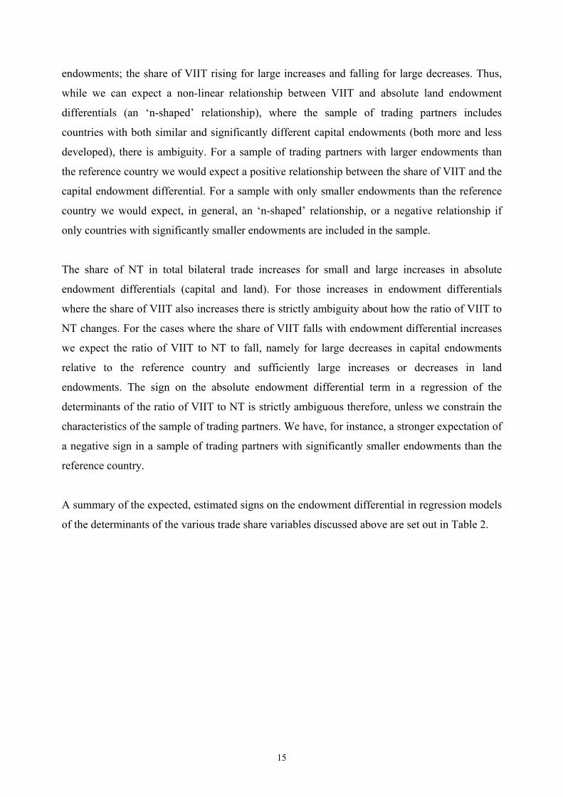
A summary of the expected, estimated signs on the endowment differential in regression models
of the determinants of the various trade share variables discussed above are set out in Table 2.
15
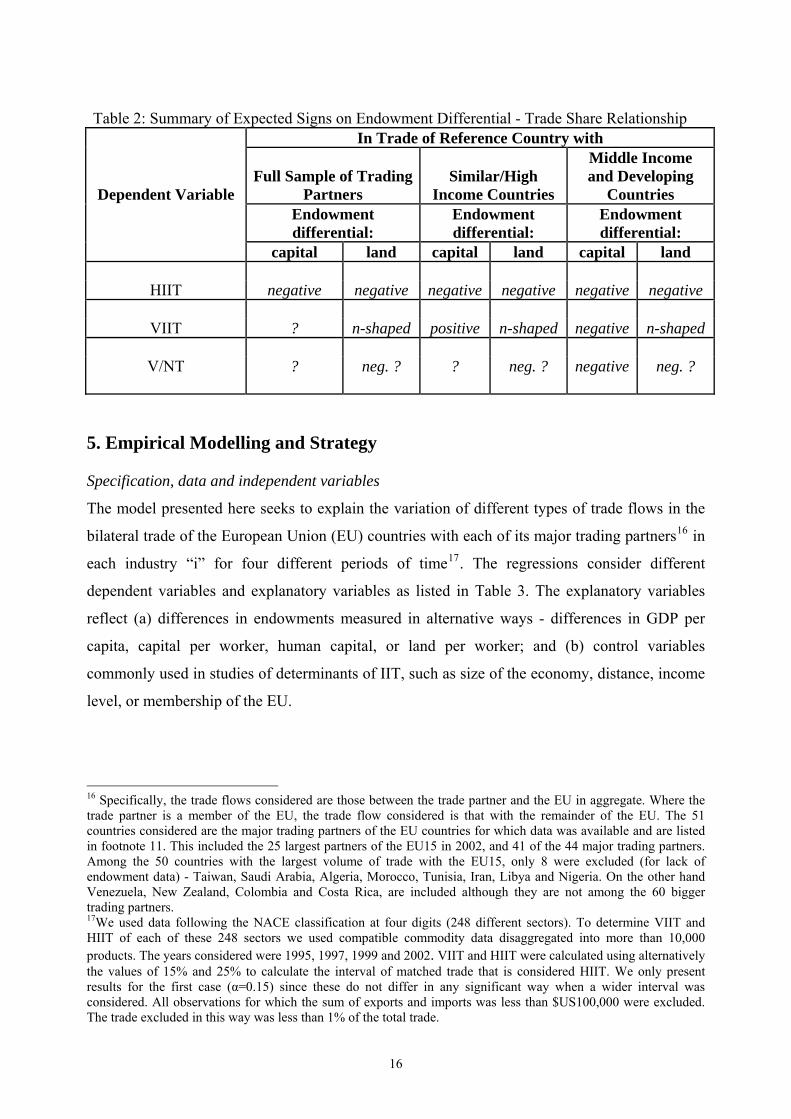
Table 2: Summary of Expected Signs on Endowment Differential - Trade Share Relationship In Trade of Reference Country with
Middle Income and Developing
Countries Full Sample of Trading
Partners Similar/High
Income Countries Dependent Variable Endowment differential:
Endowment differential:
Endowment differential:
capital land capital land capital land
negative negative negative negative negative negative HIIT ? n-shaped positive n-shaped negative n-shaped VIIT ? neg. ? ? neg. ? negative neg. ? V/NT
5. Empirical Modelling and Strategy Specification, data and independent variables
The model presented here seeks to explain the variation of different types of trade flows in the
bilateral trade of the European Union (EU) countries with each of its major trading partners16 in
each industry “i” for four different periods of time17. The regressions consider different
dependent variables and explanatory variables as listed in Table 3. The explanatory variables
reflect (a) differences in endowments measured in alternative ways - differences in GDP per
capita, capital per worker, human capital, or land per worker; and (b) control variables
commonly used in studies of determinants of IIT, such as size of the economy, distance, income
level, or membership of the EU.
16 Specifically, the trade flows considered are those between the trade partner and the EU in aggregate. Where the trade partner is a member of the EU, the trade flow considered is that with the remainder of the EU. The 51 countries considered are the major trading partners of the EU countries for which data was available and are listed in footnote 11. This included the 25 largest partners of the EU15 in 2002, and 41 of the 44 major trading partners. Among the 50 countries with the largest volume of trade with the EU15, only 8 were excluded (for lack of endowment data) - Taiwan, Saudi Arabia, Algeria, Morocco, Tunisia, Iran, Libya and Nigeria. On the other hand Venezuela, New Zealand, Colombia and Costa Rica, are included although they are not among the 60 bigger trading partners. 17We used data following the NACE classification at four digits (248 different sectors). To determine VIIT and HIIT of each of these 248 sectors we used compatible commodity data disaggregated into more than 10,000 products. The years considered were 1995, 1997, 1999 and 2002. VIIT and HIIT were calculated using alternatively the values of 15% and 25% to calculate the interval of matched trade that is considered HIIT. We only present results for the first case (α=0.15) since these do not differ in any significant way when a wider interval was considered. All observations for which the sum of exports and imports was less than $US100,000 were excluded. The trade excluded in this way was less than 1% of the total trade.
16
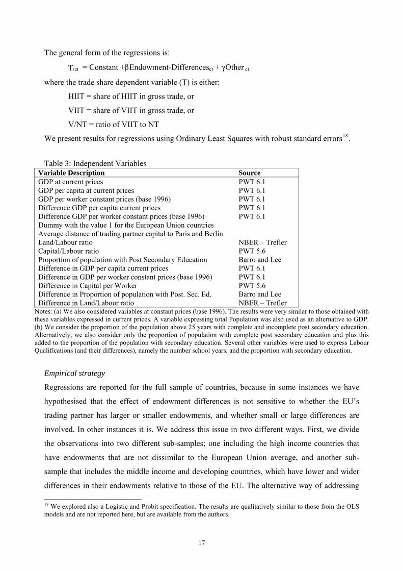
The general form of the regressions is:
Tict = Constant +βEndowment-Differences + γOtherct ct
where the trade share dependent variable (T) is either:
HIIT = share of HIIT in gross trade, or
VIIT = share of VIIT in gross trade, or
V/NT = ratio of VIIT to NT 18We present results for regressions using Ordinary Least Squares with robust standard errors .
Table 3: Independent Variables
Variable Description Source GDP at current prices PWT 6.1 GDP per capita at current prices PWT 6.1 GDP per worker constant prices (base 1996) PWT 6.1 Difference GDP per capita current prices PWT 6.1 Difference GDP per worker constant prices (base 1996) PWT 6.1 Dummy with the value 1 for the European Union countries Average distance of trading partner capital to Paris and Berlin Land/Labour ratio NBER – Trefler Capital/Labour ratio PWT 5.6
Barro and Lee Proportion of population with Post Secondary Education Difference in GDP per capita current prices PWT 6.1 Difference in GDP per worker constant prices (base 1996) PWT 6.1 Difference in Capital per Worker PWT 5.6
Barro and Lee Difference in Proportion of population with Post. Sec. Ed. Difference in Land/Labour ratio NBER – Trefler
Notes: (a) We also considered variables at constant prices (base 1996). The results were very similar to those obtained with these variables expressed in current prices. A variable expressing total Population was also used as an alternative to GDP. (b) We consider the proportion of the population above 25 years with complete and incomplete post secondary education. Alternatively, we also consider only the proportion of population with complete post secondary education and plus this added to the proportion of the population with secondary education. Several other variables were used to express Labour Qualifications (and their differences), namely the number school years, and the proportion with secondary education.
Empirical strategy
Regressions are reported for the full sample of countries, because in some instances we have
hypothesised that the effect of endowment differences is not sensitive to whether the EU’s
trading partner has larger or smaller endowments, and whether small or large differences are
involved. In other instances it is. We address this issue in two different ways. First, we divide
the observations into two different sub-samples; one including the high income countries that
have endowments that are not dissimilar to the European Union average, and another sub-
sample that includes the middle income and developing countries, which have lower and wider
differences in their endowments relative to those of the EU. The alternative way of addressing 18 We explored also a Logistic and Probit specification. The results are qualitatively similar to those from the OLS models and are not reported here, but are available from the authors.
17
this issue is to decompose VIIT into that where the EU (trade partner) is the importer (exporter)
of high quality varieties and that where the EU (trade partner) is the importer (exporter) of low
quality varieties19. We expect, from our model, that countries with higher endowments than the
EU will be exporters of high quality varieties and those with lower endowments to be exporters
of low quality varieties.
6. Regression Results
Horizontal IIT
As outlined earlier, our expectations about the sign on the endowment differences – HIIT
relationship are unambiguous and insensitive to the selection of the sample of trading partners.
A negative sign on absolute endowment differences (capital and land) is expected in a
regression of the determinants of the share of horizontal IIT for the full sample of the EU’s
trading partners. The results reported in Table 4, estimations 1 and 2 fully confirm the expected
relationship; the per capita GDP differential (eq. 2) or capital per worker differential (eq.1), and
land per worker differential (eq. 1 and 2) variables are all negative and significant. As found in
other studies of the determinants of HIIT we find strong support for a similarity thesis, namely
that the share of horizontal IIT in gross trade increases, other things constant, as endowment
differentials between countries are reduced. The signs on the other control variables are also as
expected.
For completeness we also check that the results in Table 4 are insensitive to sample selection.
In Table 5 we report the determinants of the share of HIIT estimated separately for the EU’s
bilateral trade with high income trading partners (5a) and for middle income and developing
countries (5b). Again negative signs with significance are found on all the endowment
differential variables in equations 1 and 2 for both sub-samples of trading partners.
19 A case where the value per tonne of its exports to the EU is greater than 15% of that of its imports from the EU of the same product.
18
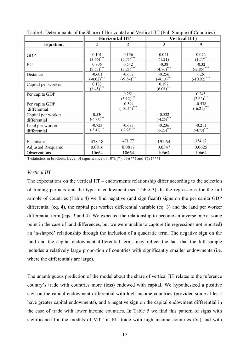
Table 4: Determinants of the Share of Horizontal and Vertical IIT (Full Sample of Countries) Horizontal IIT Vertical IIT)
Equation: 1 2 3 4
0.101 0.156 0.041 0.072 GDP (3.66)*** (5.71)*** (1.21) (1.77)*
EU 0.806 0.542 -0.38 -0.32 (9.53)*** (7.21)*** (4.76)*** (-2.85) ***
Distance -0.601 -0.652 -0.256 -1.26 (-8.02)*** (-9.34)*** (-4.13)*** (-10.92) ***
Capital per worker 0.183 0.197 (8.45)*** (6.06)***
Per capita GDP 0.251 0.245 (3.12)*** (2.62)***
Per capita GDP -0.594 -0.538 differential (-10.54)*** (-6.21)***
Capital per worker differential
-0.530 -0.532 (-3.73)*** (-4.25)***
Land per worker -0.723 -0.683 -0.236 -0.211 differential (-3.41)*** (-2.98)*** (-5.23)*** (-4.73)***
471.77 354.62 F-statistic 478.18 191.64
Adjusted R-squared 0.0816 0.0817 0.0347 0.0625 Observations 10664 10664 10664 10664 T-statistics in brackets. Level of significance of 10% (*), 5%(**) and 1% (***)
Vertical IIT
The expectations on the vertical IIT – endowments relationship differ according to the selection
of trading partners and the type of endowment (see Table 3). In the regressions for the full
sample of countries (Table 4) we find negative (and significant) signs on the per capita GDP
differential (eq. 4), the capital per worker differential variable (eq. 3) and the land per worker
differential term (eqs. 3 and 4). We expected the relationship to become an inverse one at some
point in the case of land differences, but we were unable to capture (in regressions not reported)
an ‘n-shaped’ relationship through the inclusion of a quadratic term. The negative sign on the
land and the capital endowment differential terms may reflect the fact that the full sample
includes a relatively large proportion of countries with significantly smaller endowments (i.e.
where the differentials are large).
The unambiguous prediction of the model about the share of vertical IIT relates to the reference
country’s trade with countries more (less) endowed with capital. We hypothesized a positive
sign on the capital endowment differential with high income countries (provided some at least
have greater capital endowments), and a negative sign on the capital endowment differential in
the case of trade with lower income countries. In Table 5 we find this pattern of signs with
significance for the models of VIIT in EU trade with high income countries (5a) and with
19
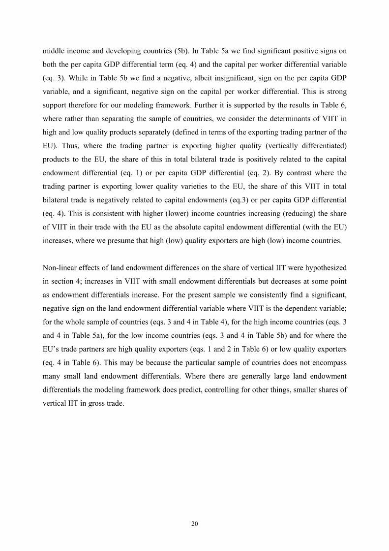
middle income and developing countries (5b). In Table 5a we find significant positive signs on
both the per capita GDP differential term (eq. 4) and the capital per worker differential variable
(eq. 3). While in Table 5b we find a negative, albeit insignificant, sign on the per capita GDP
variable, and a significant, negative sign on the capital per worker differential. This is strong
support therefore for our modeling framework. Further it is supported by the results in Table 6,
where rather than separating the sample of countries, we consider the determinants of VIIT in
high and low quality products separately (defined in terms of the exporting trading partner of the
EU). Thus, where the trading partner is exporting higher quality (vertically differentiated)
products to the EU, the share of this in total bilateral trade is positively related to the capital
endowment differential (eq. 1) or per capita GDP differential (eq. 2). By contrast where the
trading partner is exporting lower quality varieties to the EU, the share of this VIIT in total
bilateral trade is negatively related to capital endowments (eq.3) or per capita GDP differential
(eq. 4). This is consistent with higher (lower) income countries increasing (reducing) the share
of VIIT in their trade with the EU as the absolute capital endowment differential (with the EU)
increases, where we presume that high (low) quality exporters are high (low) income countries.
Non-linear effects of land endowment differences on the share of vertical IIT were hypothesized
in section 4; increases in VIIT with small endowment differentials but decreases at some point
as endowment differentials increase. For the present sample we consistently find a significant,
negative sign on the land endowment differential variable where VIIT is the dependent variable;
for the whole sample of countries (eqs. 3 and 4 in Table 4), for the high income countries (eqs. 3
and 4 in Table 5a), for the low income countries (eqs. 3 and 4 in Table 5b) and for where the
EU’s trade partners are high quality exporters (eqs. 1 and 2 in Table 6) or low quality exporters
(eq. 4 in Table 6). This may be because the particular sample of countries does not encompass
many small land endowment differentials. Where there are generally large land endowment
differentials the modeling framework does predict, controlling for other things, smaller shares of
vertical IIT in gross trade.
20
Table 5: Determinants of the Share of Horizontal and Vertical IIT: High Income and Middle Income and Developing Countries Separated a: High Income Countries HIIT HIIT VIIT VIIT
Equation: 1 2 3 4 GDP 0.229 0.219 0.150 0.110
(3.82)*** (3.67)*** (2.36)** (1.67)*
EU 0.98 0.63 0.34 0.31 (5.90)*** (3.54)*** (2.01)** (1.78)*
Distance -0.624 -1.023 -1.16 -1.22 (4.51)*** (7.56)*** (-5.52)*** (-5.63)***
Capital per worker -0.101 0.126 (-0.41) (2.12)**
Per capita GDP -0.541 0.978 (-3.13)*** (5.35)***
Per capita GDP -0.812 0.652 differential (-4.25)*** (2.88)***
Capital per worker -0.914 0.512 differential (-3.83)*** (3.12)***
Land per worker -0.131 -0.168 -0.116 -0.125 differential (-2.09)** (-2.91)*** (-1.78)* (-2.01)**
139.96 138.58 106.35 121.33 F-statistic
Adjusted R-squared 0.0511 0.0506 0.0392 0.0446 Observations 5157 5157 5157 5157
(a) For the list of countries included see footnote 11. (b) Vertical and Horizontal Grubel and Lloyd indexes (share of HIIT and of VIIT in total trade). b: Middle Income and Developing Countries HIIT HIIT VIIT VIIT
Equation: 1 2 3 4 GDP 0.007 0.037 0.127 0.189
(0.24) (1.25) (2.92)*** (4.26)***
EU 0.38 0.31 -1.18 -1.03 (3.54)*** (2.92)*** (-9.11)*** (-8.15)***
Distance -0.287 -0.220 -0.105 -0.115 (-3.71)*** (2.82)*** (-10.25)*** (11.17)***
Capital per worker 0.132 0.142 (3.27)*** (3.86)***
Per capita GDP 0.659 1.12 (5.34)*** (7.31)***
Per capita GDP -1.17 -0.101 (-7.55)*** (-0.53) differential
Capital per worker -0.480 -1.56 differential (-3.42)*** (-3.23)***
Land per worker -0.226 -0.198 -0.875 -0.794 differential (-5.40)*** (-4.81)*** (-16.32)*** (-14.77)***
78.36 102.45 259.28 265.25 F-statistic
Adjusted R-squared 0.0276 0.0359 0.0867 0.0885 Observations 5444 5444 5444 5444
T-statistics in brackets. Level of significance of 10% (*), 5%(**) and 1% (***)
21
Ratio of vertical IIT to net trade
Where the share of vertical IIT falls with increasing endowment differentials we expect also the
ratio of vertical IIT to net trade to fall. We find support for this in the results of the determinants
of V/NT in Table 7. The sign on the land per worker differential is negative and significant for
all the specifications in this table. Although there is strictly ambiguity about the relative changes
in the shares of VIIT and NT as capital endowment differences change (especially for trade with
countries with greater incomes or capital endowments), it is the case that VIIT should decrease
after some point for endowment differential increases with countries with lower incomes or
capital endowments. In which case, in sample of countries with a substantial proportion of lower
income countries one would expect there to be an inverse relationship overall between the
VIIT/NT ratio and absolute endowment differences. This is what we find for the full sample of
trading partners in Table 7. Both the proxies for the capital endowment differential (per capita
GDP differential and capital per worker differential) have a negative sign with significance
(even after trying to control for large endowment difference effects through the inclusion of
dummies).
22
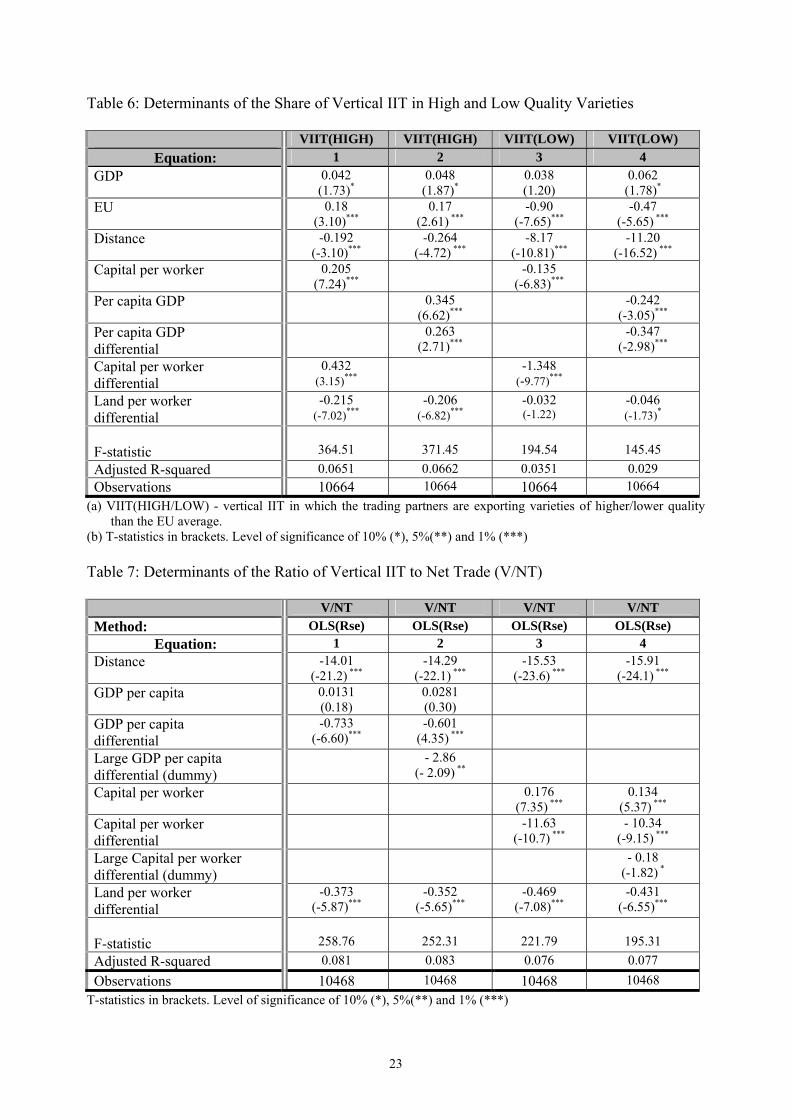
Table 6: Determinants of the Share of Vertical IIT in High and Low Quality Varieties VIIT(HIGH) VIIT(HIGH) VIIT(LOW) VIIT(LOW)
Equation: 1 2 3 4 GDP 0.042 0.048 0.038 0.062
(1.73)* (1.87)* (1.20) (1.78)*
EU 0.18 0.17 -0.90 -0.47 (3.10)*** (2.61) *** (-7.65)*** (-5.65) ***
Distance -0.192 -0.264 -8.17 -11.20 (-3.10)*** (-4.72) *** (-10.81)*** (-16.52) ***
Capital per worker 0.205 -0.135 (7.24)*** (-6.83)***
Per capita GDP 0.345 -0.242 (6.62)*** (-3.05)***
Per capita GDP 0.263 -0.347 differential (2.71)*** (-2.98)***
Capital per worker 0.432 -1.348 differential (3.15)*** (-9.77)***
Land per worker -0.215 -0.206 -0.032 -0.046 (-1.22) differential (-7.02)*** (-6.82)*** (-1.73)*
364.51 371.45 194.54 145.45 F-statistic
Adjusted R-squared 0.0651 0.0662 0.0351 0.029 Observations 10664 10664 10664 10664
(a) VIIT(HIGH/LOW) - vertical IIT in which the trading partners are exporting varieties of higher/lower quality than the EU average.
(b) T-statistics in brackets. Level of significance of 10% (*), 5%(**) and 1% (***)
Table 7: Determinants of the Ratio of Vertical IIT to Net Trade (V/NT) V/NT V/NT V/NT V/NT Method: OLS(Rse) OLS(Rse) OLS(Rse) OLS(Rse)
Equation: 1 2 3 4 Distance -14.01 -14.29 -15.53 -15.91
(-21.2) *** (-22.1) *** (-23.6) *** (-24.1) ***
GDP per capita 0.0131 0.0281 (0.18) (0.30)
GDP per capita -0.733 -0.601 differential (-6.60)*** (4.35) ***
Large GDP per capita - 2.86 (- 2.09) **differential (dummy)
Capital per worker 0.176 0.134 (7.35) *** (5.37) ***
Capital per worker -11.63 - 10.34 differential (-10.7) *** (-9.15) ***
Large Capital per worker - 0.18 (-1.82) *differential (dummy)
Land per worker -0.373 -0.352 -0.469 -0.431 differential (-5.87)*** (-5.65)*** (-7.08)*** (-6.55)***
258.76 252.31 221.79 195.31 F-statistic
Adjusted R-squared 0.081 0.083 0.076 0.077 Observations 10468 10468 10468 10468
T-statistics in brackets. Level of significance of 10% (*), 5%(**) and 1% (***)
23
7. Conclusions Our main aim in this paper has been to investigate, both theoretically and empirically, the
relationship between endowment differences and the share of intra-industry trade. This was
partly prompted by the contradictory empirical evidence on the effects of endowment
differences on vertical intra-industry trade, with some authors finding a positive and others a
negative relationship. To this end we constructed an illustrative theoretical model from which
we drew inferences on the implications of small and large endowment differences for the shares
of horizontal and vertical intra-industry trade. The predictions for horizontal intra-industry trade
were quite conventional - that larger endowment differences would reduce such trade. But the
predictions for vertical intra-industry trade were more factor and trading partner specific. The
model predicted that vertical intra-industry trade would grow with differences in specific factor
endowments, as long as these differences remain small. The effects of larger specific factor
endowment differences depend on whether the specific factor is used by the industry. If not,
then VIIT declines for larger endowment differences. If so, then the share of VIIT increases
(decreases) if the trading partner has an ever larger (smaller) endowment. Our results on EU
trade confirmed that horizontal intra-industry trade declines with growing endowment
differences. They also confirmed the sensitivity of vertical intra-industry trade flows to the
magnitude of endowment differences. The specific predictions on endowment differences in the
specific factor used by the industry (assumed to be capital) were also confirmed. But the
nonlinearities predicted for the other specific factor (assumed to be land) did not appear, perhaps
due to insufficient variability in the sample.
These findings help to resolve the uncertainty that had arisen from earlier work on how vertical
IIT varies with endowment differences. Because of its dominance in North-North trade it might
be viewed as being affected by endowment differences in the same way as horizontal IIT.
Equally the theoretical models of vertical IIT in North-South trade suggest a similar influence of
endowment differences on both vertical ITT and inter- or net trade. Here we find a difference in
the way endowments affect vertical IIT from both horizontal IIT and net or inter-industry trade.
The share of horizontal IIT decreases for all increases in absolute endowment increases and the
share of net trade increases for all increases in endowment differences with trading partners, but
the share of vertical IIT both increases and decreases with increases in specific endowment
differences. This finding supports the view that both within and between industry specialization
24
and trade can be driven by factor endowment considerations, and undermines the view that
vertical IIT is simply disguised H-O trade associated with industry (mis)aggregation.
25
REFERENCES
Abn-el-Rahman, K. (1991), ‘Firms’ Competitive Advantages as Joint Determinants of Trade Composition’, Review of World Economics, 127, 83-97.
Blanes, V. and C. Martin (2000), ‘The Nature and Causes of Intra-Industry Trade: Back to the Comparative Advantage Explanation? The Case of Spain’, Review of World Economics, 136, 423-41.
Cabral, M., Falvey, R. and C. Milner (2006), ‘The Skill Content of Inter- and Intra-Industry Trade: Evidence for the UK’, Review of World Economics, 142, 546-66.
Crespo, Nuno and Fontoura, Maria Paula (2001), ‘Determinants of the Pattern of Horizontal and Vertical Intra-Industry Trade: What Can We Learn From Portuguese Data?’, Mimeo, ISEG Technical University of Lisbon.
Davis, D. D. (1995) “Intra-industry trade: A Heckscher-Ohlin-Ricardo approach” Journal of International Economics 39, 201-226.
Deardorff, A. (1984), ‘An Exposition of Krueger’s Trade Model’, Canadian Journal of
Economics, 17, 731-46.
Durkin, John T. and Krygier, Markus (2000), ‘Differences in GDP Per Capita and the Share of Intra-industry Trade: The Role of Vertically Differentiated Trade’, Review of International Economics; 8, 760-74.
Falvey, R. E. (1981), ‘Commercial Policy and Intra-Industry Trade’, Journal of International Economics, 11, 495-511.
Falvey, R. E. and H. Kierzkowski, (1987), ‘Product Quality, Intra-industry Trade and (Im)perfect Competition’, in Henryk Kierzkowski (ed.), Protection and Competition in International Trade, Basil Blackwell, Oxford, Chapter II.
Fukao, K, Ishido, H, Ito, K (2003), ‘Vertical Intra-industry Trade and Foreign Direct Investment in East Asia’, The Institute of Economic Researsh, Hitotsubashi University Discussion Paper, nº 434, Series A.
Gabrisch, H. and Segnana (2002), ‘Intra-Industry Trade between European Union and the Transition Economies. Does Income Distribution matter?’, LIS Working Paper , Nº 297.
Greenaway, David, Hine, R.C. and Milner, Chris (1994), ‘Country-Specific Factors and Pattern of Horizontal and Vertical Intra-industry Trade in the UK’, Review of World Economics, 130, 77-100.
Greenaway, David, Hine, R.C. and Milner, Chris (1995), ‘Vertical and Horizontal Intra-industry Trade: A Cross Industry Analysis for The United Kingdom’, Economic Journal, 105, 1505-18.
Greenaway, David, Milner, Chris and Elliott, Robert (1999), ‘UK Intra-Industry Trade with the EU North and South’, Oxford Bulletin of Economics and Statistics, 61, 364-84.
Gullstrand, Joakim (2000), ‘Country-Specific Determinants of Vertical Intra-Industry Trade With Application to Trade Between Poland and EU’, in B. Wawrzynjak (ed.), Globalisation and Change – Ways to Future, Leon Kozminski Academy of Enterpreneurship and Management, Warsaw.
26
Helpman, Elhanan (1981), ‘International Trade in the Presence of Product Differentiation, Economies of Scale and Monopolistic Competition’, Journal of International Economics, 11, 305-340
Helpman, Elhanan and Krugman, Paul R.(1985), Market Structure and Foreign Trade - Increasing Returns, Imperfect Competition and the International Economy, Mass, MIT Press, Cambridge.
Hummels, D. and Levinsohn, J. (1995), ‘Monopolistic Competition and International Trade: Reconsidering the Evidence’, Quarterly Journal of Economics, 110, 799- 836.
Krueger, A.O. (1977), Growth Distortions and Patterns of Trade Among Many Countries, Princeton Studies in International Finance, No: 40, (Princeton, NJ, Princton University).
Krugman, Paul R. (1979), ‘Increasing Returns, Monopolistic Competition and International Trade’, Journal of International Economics, 9, 469-79.
Martin-Montaner, J. A. and Orts Rios, Vicente (2002), ‘Vertical Specialization and Intra-Industry Trade: The Role of Factor Endowments’, Review of World Economics, 138, 340-365.
Nielsen, J.U.-M., and Luthje, T. (2002), ‘Tests of Empirical Classification of Horizontal and Vertical Intra-Industry Trade’, Review of World Economics, 138, 587-604.
27