RESEARCH PAPER Directed Movements in Probabilistic Time Geography · Time geography represents the reachable locations of this agent by a space-time cone, a right cone in x-y-t-space

January 16, 2010 7:37 Journal of Geographical Information Science winter09probabilistic-final

Journal of Geographical Information ScienceVol. 00, No. 00, January 2008, 1–17

RESEARCH PAPER

Directed Movements in Probabilistic Time Geography

Stephan Wintera∗ and Zhang-Cai Yina,b

aDepartment of Geomatics, The University of Melbourne, Australia;bSchool of Resources and Environmental Engineering, Wuhan University of Technology,

China;

(January 16, 2010)

This paper studies probabilistic time geography for space-time prisms, i.e., for situationswhere observers know the location of an agent at one time and then again at another time.In between the agent has moved freely, according to its time budget. The paper demonstratesthat the probability to find the agent somewhere in the space-time prism is not equallydistributed, such that any attempt of a quantitative time geographic analysis must considerthe actual probability distribution. This distribution is developed in this paper, implementedand demonstrated. The paper is a second, after introducing first probabilistic time geographyfor space-time cones. With cones and prisms, the elementary space-time volumes of timegeography are provided.

Keywords: probabilistic time geography; uncertainty; spatiotemporal reasoning; movingobjects

1. Introduction

Probabilistic time geography accepts likelihoods for the location of an agent ata particular time. In a space-time aquarium formed by (x, y, t) the tradition-ally Boolean space-time volumes of time geography in isotropic space—cones andprisms—can, in a probabilistic approach, be replaced by clouds of probability dis-tributions. Analytically these clouds can be computed by probability distributionsat any time instance, and between time instances there are correlations: if a mobileagent is most likely at time t at a particular location, then at time t + ∆t thisagent is most likely still nearby. This means, we expect continuous distributions ofprobabilities over time within these clouds.

In a previous paper the concept of probabilistic time geography was introduced(Winter 2009). It was demonstrated how these correlations over time can be mod-eled in a discrete, voxel-based space-time cone by iterative computations of theprobability values. The individual probabilities in each cell, characterizing the like-lihood of the agent being in this cell at this time t, allow elementary forms ofreasoning. By this way it was possible to say, for example, how likely it is to findagent a at time t at a discrete location (x, y) or in an area

∑(x, y), or how likely it

is that two agents a and b are in the same location at t. The computation of suchprobabilities in a discrete space-time cone turned out to be efficient.

∗Corresponding author. Email: [email protected]

ISSN: 1365-8816 print/ISSN 1362-3087 onlinec© 2008 Taylor & FrancisDOI: 10.1080/1365881YYxxxxxxxxhttp://www.informaworld.com


2 Winter and Yin

So far, however, the elementary theory of probabilistic time geography consistsonly of measures dealing with uncertain space-time cones. This paper will extendthese first steps by two significant improvements. First, it will study probabilisticspace-time prisms. Cones are the volumes in time geography where an agent’s max-imum speed and their location at a time ts are known, and nothing else. Prismsmodel in time geography the volume where in addition to the previous also theagent’s location at a time te, te > ts, is known, and nothing else. Requiring thisadditional knowledge the computation of space-time prisms is of course only possi-ble in hindsight, probabilistic or not. However, in probabilistic time geography thisadditional knowledge is also impacting the local probabilities. We will develop herethe mathematical foundations to compute these probabilistic space-time prisms.Secondly, in our pursuit to develop these foundations we also extend the discretevoxel-based model of recursive computations by direct computations on a continu-ous time scale, now being able to compute the probability distribution at any timet ∈ R. As a result, we will have a complete theory for probabilistic time geographyin an isotropic space.

The paper is structured as follows. Section 2 summarizes the previous paper(Winter 2009), including the references to classical time geography. Then we pro-ceed to directed movements (Section 3), or movements between two known loca-tions. The developed model to compute these probabilistic space-time prisms willbe implemented and tested in Matlab in Section 4. Conclusions close the paper(Section 5).

2. Background

This section summarizes a preliminary introduction of probabilistic time geography(Winter 2009), which was exploring the first principles of the theory for simplespace-time cones. These first insights are also related to the further contributions ofthis paper. Probabilistic time geography was suggested as an extension of (classical)time geography (Hagerstrand 1970), based on random walks. Random walks forspace-time cones were unbiased ones, where nothing else is known or assumed thanthe location of an agent at a particular time and its maximum velocity. This paperwill introduce biased random walks, to reflect the additional knowledge comingwith space-time prisms that the agent is at a later time at another registeredlocation.

2.1. Time geography

Time geography answers questions such as: Given a location of a mobile agentat ts, where is the agent at a later time t > ts? Or where was it at a past timet < ts? Assume that the agent can move in any direction and is limited only by amaximum speed. Time geography represents the reachable locations of this agentby a space-time cone, a right cone in x-y-t-space. The cone apex represents theagent’s location at ts, and the aperture the maximum speed of the agent, such thata cone base represents the set of locations the agent may settle at a time t > ts(Figure 1a), and similarly for t < ts.

Time geographic models of movements where start and destination are knownare sketched in Figure 2. For sufficiently dense tracking data (see the samplingtheorem Shannon and Weaver 1949), as assumed for example in moving objectdatabases (Guting and Schneider 2005), a linear interpolation might be sufficient(Fig. 2a). However, a complete model, as provided by time geography, captures also


International Journal of Geographical Information Science 3

Figure 1. Traditional time geography concepts.

Figure 2. Time geographic concepts of directed movement: (a) linear interpolation, (b) straight space-timeprism, (c) oblique space-time prism, (d) probabilistic space-time prism.

all the possible intermediate locations by an oblique or even a straight space-timeprism. So if the agent’s location is known at ts and then again at te, the possiblyreachable volume is described by a cone with apex in ts, reduced by the intersectionwith an inverse cone with an apex at te. This space-time prism (Hagerstrand 1970)(sometimes called bead (Hornsby and Egenhofer 2002)) is straight if the agentreturns at te to the location of the origin at ts (Fig. 2b); otherwise it is oblique(Fig. 2c).

Miller (1991) maps space-time prisms to network spaces, considering link-basedtravel speeds in a transportation system. Note that volumes reduce to vertical sec-tions if travel is constrained on linear paths. Time geography was also implementedin GIS for the analysis and visualization of access for individuals, and long-termmovement patterns (e.g., Kwan 2004, Shaw and Yu 2009). A survey of applicationsof time geography is beyond the scope of this paper; here it is only important tonote that time geography so far stayed qualitative in modeling and analyzing thesespace-time volumes.

The basic qualitative question is simply where an agent A may be located aftersome time, let us say, at time t. To answer this question, only the base of thespace-time volume at t has to be computed. Derived qualitative questions con-cern multiple agents. Examples are whether an agent A has possibly met agentB (Figure 1b), or whether agent A has possibly reached the location of an immo-bile agent or object C (Figure 1c). The immobile agent or object is also called aspace-time station in time geography. A space-time station is a degenerated cone ofzero aperture. Some derived qualitative questions are answered by testing whetherthe agents’ space-time volumes intersect, which is a relative complex computation.Other derived qualitative questions are simpler to answer, just by testing whetherthe bases of the space-time volumes at time t intersect.

For the qualitative analysis of intersections one can apply the usual relational cal-culi for extended objects: the 9-intersection model (Egenhofer and Herring 1991),or the region connection calculus (Randell et al. 1992). Even extensions for uncer-tain objects exist of these calculi (Winter and Bittner 2002, Cohn and Gotts 1996,Clementini and Di Felice 1996, Neutens et al. 2007b), in case we would like toextend crisp space-time volumes by uncertain ones. However, the qualitative state-ments derived from these calculi have to consider the point-like nature of the agents


4 Winter and Yin

that are described by the space-time volumes. This means all the possible topolog-ical relationships have to be mapped onto the only distinguishable 0-dimensionalrelationship, meet, and its qualitative likelihoods: impossible or possible.

Questions involving quantification were not suggested so far. An exception maybe Neutens et al. (2007a) who suggest a fuzzy space-time volume, but not yetdeveloping the analysis tools. Quantitative questions would be of the kind: Whatis the most probable arrival time of A at C? Or what is the probability that A andB have met by time t? Or, if A searches at ts for a collision-free travel in a withagents populated environment, what is the safest path? Generally, a quantificationwould require assumptions on the probability of an agent’s presence at particularlocations within its space-time volume. A naive approach would assume a uniformprobability distribution over sections of space-time volumes, and simply computerelative sizes of intersection. But this assumption is wrong as we will explain later.Figure 2d sketches a space-time prism with a non-uniform probability distribution.

2.2. Random walks

Unknown movements of agents can be modeled as random walks. These randomwalks would be unbiased in absence of any evidence to assume otherwise, or bi-ased if such evidence exists. An unbiased random walk models continuous diffusionprocesses such as Brownian motion, which is approximating sufficiently the goal-oriented behavior of (bounded) rational agents (Rubinstein 1998) only over largetime spans. On smaller time spans the behavior of rational agents appears to bemore directed and, frequently, regular (Bovy and Stern 1990). We will model thisbehavior by biased random walks. A bias can easily brought in existing randomwalk models by biased transition probabilities, but biased random walks have notfound much attention in the literature.

For infinite random walks in one- and two-dimensional discrete space the like-lihood of an agent returning to the origin (or, equivalently, reaching any otherparticular point in space) is always 1 (Polya 1921). However, in this paper we aremore interested in finite time spans, as they occur in time geography, and hence, weexpect probabilities of an agent reaching a particular location smaller than 1. Fur-thermore, a finite partition of space guarantees probabilities of agents at particularlocations larger than 0.

Random walks are also used to model the behavior of large numbers of mo-bile agents. For example, transportation research simulates by random walks largenumbers of mobile agents to study higher order patterns such as flocking behavior,crowding, queuing or congestions (e.g., Batty 2003, Hoogendoorn and Bovy 2003,Balmer et al. 2004), and in sensor network research they are deployed to estab-lish a population of mobile sensor nodes that then can be studied for their ad-hoccommunication behavior (e.g., Camp et al. 2002).

In contrast, here random walks simulate the many wayfinding options a singleagent has. Large numbers of random walk simulations provide frequencies of vis-ited places at particular times, which can be normed to probabilities. Besides ofagent-based simulation, also combinatorics or convolution can be used to repre-sent random walks mathematically. The following section summarizes how Winter(2009) introduced probabilistic time geography for unbiased movements, using theapproach by convolution.



2.3. Probabilistic time geography

Let us study an agent A with a known location at ts and a known maximum speed.For this purpose, an isotropic discrete space-time aquarium was assumed that isregularly partitioned into voxels of (∆x, ∆y, ∆t). The agent starts at ts movingfrom a known location, and ending at te after n time steps of a priori unknownmovements. The discrete steps of the agent are limited by its maximum speedvmax. Assume a discrete vmax = 1, which always can be realized by choosing asuited temporal resolution ∆t, and a distance measure based on 4-neighborhood.Then in one time interval the agent can move to the South, North, West, or Eastneighbor of its actual location, or it can stay where it is (Fig. 3). Thus a randomwalk consists of a sequence of a pair of actions in each time interval: a randomassignment of a heading, and a move according to the actual heading. The randomassignment of the heading is chosen unbiased because no prior knowledge of theagent’s goal exists.

Figure 3. A random walk of vmax = 1 in discrete space.

Expressing this random walk behavior by convolution is straight forward. Imagineat ts an agent in (xs, ys) in an otherwise empty discrete spatial field g: a unit impulsefunction. The convolution, or discrete linear spatial filtering of g by a kernel h, isgiven by:

g′x,y = gx,y ⊗ h =∞∑

i=−∞

∞∑

j=−∞hi,j gx−i,y−j (1)

with g′ the resulting filtered spatial field at time ts+1. In this most general ex-pression of a convolution, the neighborhood of a focal point (x, y) is unlimited(−∞ . . .∞), but in practical applications its area of influence can be limited to asmall neighborhood, supported by Tobler’s law: “Everything is related to every-thing else, but near things are more related than distant things.” (Tobler 1970,p. 236). A typical size of a kernel is only 3 × 3, describing the neighborhood of afocal point from (x− 1, y − 1) to (x + 1, y + 1). We say this kernel has a radius ofd = 1. In the present context, however, the reason to limit the kernel to a radiusof 1 is given by the maximum speed vmax of the agent.

The 3 × 3 convolution kernel h reflecting the above described discrete randomwalk is:

h =

0 1 01 1 10 1 0

(2)


6 Winter and Yin

Applied recursively on the unit impulse function at (xs, ys) the collected convolu-tions at the discrete times ts+i provide frequencies of visits of locations. At timets+1 the result g′ = g1 equals an image of h, indicating equal probability for atransition from (xs, ys) to any of its neighbors, or to stay, and at time ts+2 theresult g′′ = g2 would already be:

. . . . . . . . . . . . . . . . . . . . . . . . . . .

. . . . . . . . . . . . 0 . . . . . . . . . . . .

. . . . . . . . . 0 1 0 . . . . . . . . .

. . . . . . 0 1 2 1 0 . . . . . .

. . . 0 1 2 3 2 1 0 . . .

. . . . . . 0 1 2 1 0 . . . . . .

. . . . . . . . . 0 1 0 . . . . . . . . .

. . . . . . . . . . . . 0 . . . . . . . . . . . .

. . . . . . . . . . . . . . . . . . . . . . . . . . .

indicating that more random movements would lead through (x0, y0) than throughany other cell. Now, using a normalized kernel:

h′ =15h (3)

provides directly the probabilities of visits, instead their frequencies (Fig. 4). Forexample, the probability for an agent to stay between ts and ts+1 in (xs, ys) is 0.2,as it is for reaching any of its four neighbors. Only the second convolution providesmore differentiated probabilities, where the intensity in grey is proportional to theprobability value.

Figure 4. The normalized convolution kernel (left) and the probability distribution of locations of a mobileagent at two sequential time steps (right).

A careful recursive formulation of the convolution further avoids the computationof values for empty cells: the cells outside of the space-time volume. If the convo-lution is only computed for the voxels within the cylinder enclosing the space-timecone, then still 75% of all cells in the cylinder are empty. Thus, for an agent beinglocated at (xs, ys) at ts the space-time cone between ts and te consists of a discretenumber n of layers computed by this limited and recursive convolution:

gx,y,k ={

0 if max(|x− xs|, |y − ys|) > kgx,y,k−1 ⊗ h else (4)

This means the computational complexity of the recursive convolution is a functionof time only, more precisely, of the number of time intervals for which a cone iscomputed. For each time step i the convolution computes (2i + 1)2 new values(O(n2)).



3. Biased random movement

Up to now the knowledge of an analyst was limited to three parameters: the locationof an agent at a time ts, (xs, ys), and its maximum speed. Due to lack of any otherknowledge all directions of traveling were considered equally likely for an agent’smove. Thus, the computations so far are sufficient to replace traditional space-timecones by probabilistic ones. But with additional knowledge, e.g., the location of theagent at a later point in time, these assumptions have to be revised, including theprobabilistic representation and reasoning model. This extension will be introducedhere.

3.1. From cones to prisms

If the location of an agent at a time ts is known, and then at te again, traditionaltime geography combines two space-time cones to space-time prisms (Figures 2b–c). Formally, the movement is from a start location to an end location, although—depending on the time budget—the agent can travel substantial deviations fromthe direct route between the two locations. The agent even may not call the firstlocation the start or the second the end, since these two observations can have beenmade at any time during a continuous movement of the agent. Nevertheless, withthe knowledge of a start and an end location we can say the agent has a generalheading between ts and te. At least on average the agent’s travel parameters aredetermined by (a) the direction from start to end, and (b) the expected or averagespeed v coming out of the proportion of the distance between start and end andthe time interval te − ts. The average speed v must be smaller than vmax for theagent being able to reach the end location within this time frame, or if v = vmax

then the prism degenerates to a straight line.Such assumptions are worth to be discussed further. They are bare of any further

world knowledge of the traveling agent, or of any world conditions or constraints.Further knowledge would be likely require to modify these assumptions. For in-stance, if the environment offers preferential routes, or various modes of traveling,or if the maximum speed is restricted variably across the environment, these as-sumptions do no longer hold. They are, from a probabilistic perspective and dueto the central limit theorem, only true for an isotropic space and a large numberof random walking agents between (xs, ys, ts) and (xe, ye, te).

To determine a probabilistic space-time prism (Figure 2d, or more detailed Fig-ure 5) one can follow the previous argument for a computation by convolutionson a discrete grid network. In line with Section 2.3, a (probabilistic) space-timeprism g in the grid network is the time-expanded set of possible paths betweenstart and end. It can be computed from two cones gs and ge, one from each apex,and progressing towards each other, i.e., gs growing from the start at ts towardste, and ge from the end at te towards ts. This way, the two cones permeate eachother. Since together they describe one phenomenon—the movement of a singleagent—they also constrain each other. Hence, they have to be intersected by thefollowing rule:

gx,y,k ={

max(gsx,y,k, ge

x,y,k) if gsx,y,k · ge

x,y,k > 00 else

(5)

saying the probability of finding an agent at a location that is outside of one ofthe cones is a priori 0, and the probability within the volume where gs and ge

intersect is the larger probability of both cones. For example, close at (xs, ys, ts)


8 Winter and Yin

Figure 5. The agent’s potential path area (PPA) from the space-time prism.

the probability from gs will be quite large and the one from ge low.This rule reflects also the point symmetry about the central point between start

and end location. This means, the computation of g can be shortened by acknowl-edging this symmetry. Consider the two apexes (xs, ys, ts) and (xe, ye, te) formingthe datums of two local coordinate systems. Then, with the translation constants∆x = xe − xs, ∆y = ye − ys and ∆t = n (for n discrete time steps), in the aboveEquation 5 ge

x,y,k can be replaced by:

gex,y,k = gs

x+∆x,y+∆y,k+∆t (6)

However, the general heading of the agent violates the assumption of uniformtransition probabilities. For unbiased movements, the potential path area, whichis the set of geographic locations that the agent can have visited between ts andte Miller (1991, p. 291), is circular—the projection of the cone to the x-y-plane.But with a biased movement the potential path area is no longer circular, butelliptic(Figure 5)—the projection of the prism to the x-y-plane—, with the twofoci of the ellipse in the start and end locations. Direction requires a re-thinkingthrough probability distributions.

3.2. Introducing a direction

The knowledge that the agent has moved from (xs, ys, ts) (the start location atts) to (xd, yd, te) (the end location at te) implies a general heading of the agent ina particular direction, which violates the assumption of uniform transition prob-abilities from Equation 3. Instead, this additional knowledge of a bias towards aparticular direction can be expressed by a correspondingly non-uniform probabilitydistribution. With this additional knowledge the best guess for transition proba-bilities is a linear movement from start to end (Fig. 2a, also present in Fig. 5), themovement of lowest energy and also the movement of lowest description length.

Then, according to Figure 6, the heading of the agent can be computed fromstart location and end location:

λ = arctan∆y

∆x(7)

φ = arccot

√∆x2 + ∆y2

∆t(8)

Herein, λ represents the longitude and φ the latitude of the end from the start.Equation 7 has a singularity at ∆x = 0, at which λ is π

2 ,−π2 , or even 0, depending on

the sign of ∆y. Because of the directed time axis φ can only be positive, 0 < φ ≤ π2 .

In fact, the agent has a maximum speed vmax which sets the lower bound for φ,



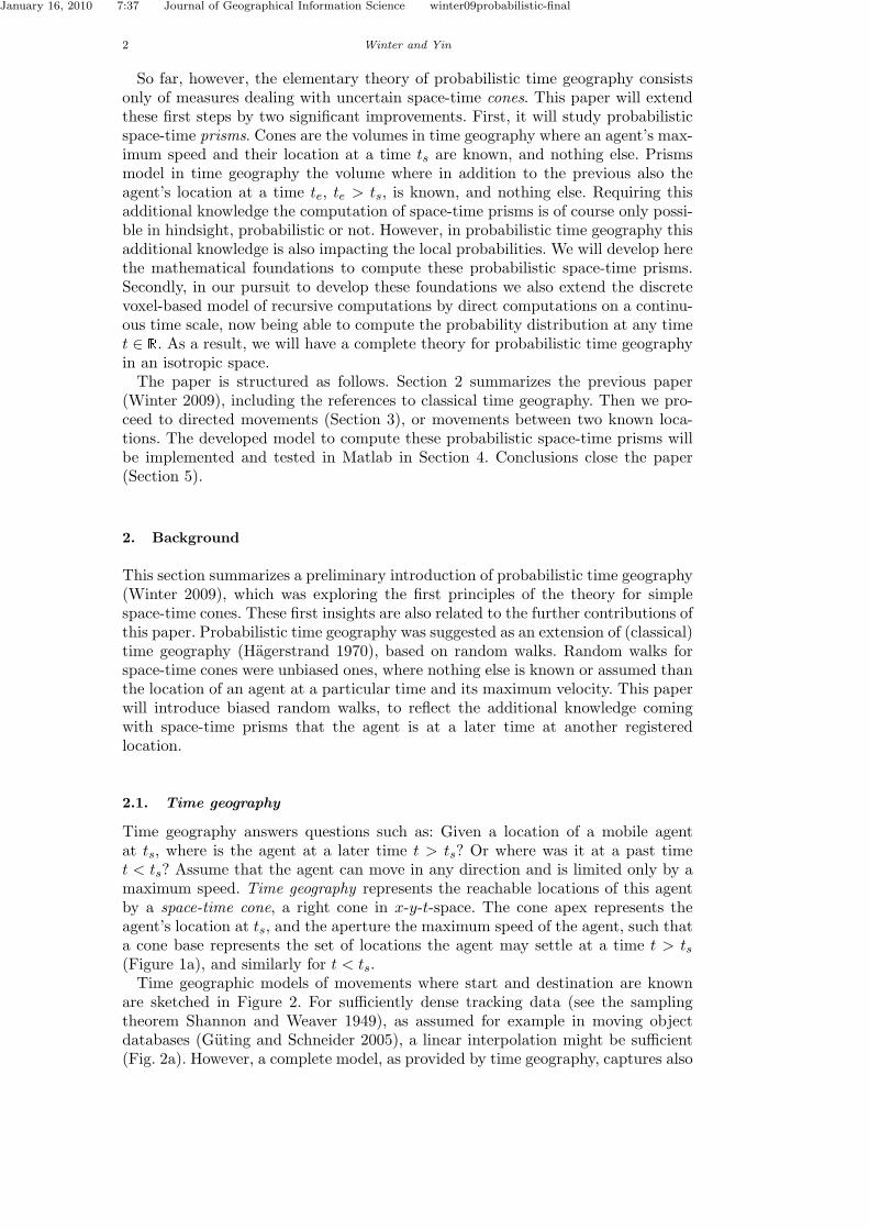
Figure 6. An agent heading towards a destination.

and if we choose a temporal resolution such that vmax = 1, as we did above, thenπ4 ≤ φ ≤ π

2 . Thus, for any ∆t > 0 Equation 8 has no singularity.Now see again Figure 6: Moving from the start (xs, ys, ts) along the vector (λ, φ)

for some time t leads to the average intermediate location µt = (µx, µy) relativeto xs, ys. The location µt is the one where the agent is expected to be found att with highest likelihood, according to the global knowledge to find this agent atte at xe, ye and the general behavior of a random walker. With this intermediatetravel time t somewhere between ts and te, tx < t ≤ te, the distance of µt from(xs, ys), dµ, can be computed by:

dµ = cotφ · (t− ts) = v · (t− ts) (9)

With dµ we can compute the components of µ at time t:

µt = (µx, µy)t = (dµ cosλ, dµ sinλ)t (10)

3.3. Introducing a probability distribution

To model the average movement along µt requires biased transition probabilitiesof a random walker towards µt, and hence, Equation 3 does no longer hold. Fur-thermore, the probability distribution at each time t must (continue to) be finite,limited to the base of the space-time prism at t. The following considerations andformulas continue to be applicable to the discrete space-time aquarium, but arealso generic enough to be computed at any time on a continuous time scale. Thus,from now on we will no longer stick to a discrete space-time aquarium.

A non-uniform probability distribution comes with a mean at µt, but still has notmuch reason to be asymmetric. One reason to expect symmetry is that the base atany time t is symmetric. The other reason again goes back to the random walkingmodel: there is statistically no reason to assume that an agent is locally more likelyto be faster than slower (a wave-shaped distribution) compared to average speed,or has a stronger preference to make right turns than left turns along the route. Toapproximate this finite distribution over the base the bivariate normal distributionis chosen. Since this approximation is of infinite domain, a clipping to the baseand a normalization step will be added. This bivariate normal distribution willbe centered at µ, and spreads with a variance-covariance matrix Σ. Since both, µand also Σ (as will be shown later), are functions of time, this bivariate normal


10 Winter and Yin

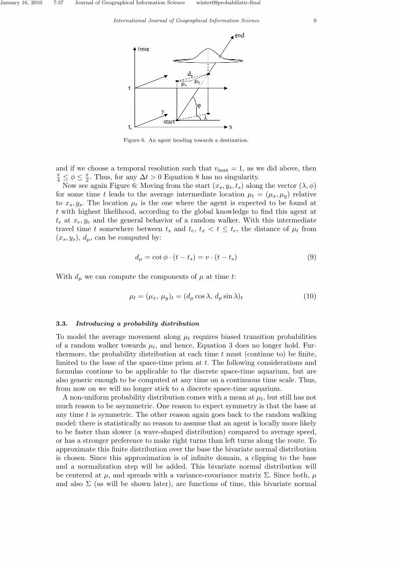
Figure 7. Parameters to compute elements of the space-time prism.

distribution is a function of time:

ft =1

2π√|Σ|e

− (x−µ)′Σ−1(x−µ)2 (11)

Next the potential path area is developed, then the clipping of the distribution,and finally the variance-covariance matrix of the bivariate normal distribution.

3.3.1. The potential path area

Finiteness at each time extends to finiteness over the whole period te − ts, de-scribed by the potential path area:

• If start and end location are identical, i.e., dµ = 0, the potential path arearemains a circle.• If start and end location do not coincide, the potential path area forms an

ellipse.• With the maximum biased movement of vmax = 1 (φ = π

4 ) the agent has noother choice than heading with maximal speed in the direction of λ. Practicallythis means complete knowledge of the agent’s trajectory, or a probability of 1 atµ, and 0 everywhere else. The potential path area degenerates to a line.

Figure 7 shows a typical space-time prism with an elliptic potential path area. Thesemifocus c of the ellipse, which is half of the distance between the foci, is:

c =|F1F2|

2(12)

The semimajor axis of the ellipse follows as:

a =vmax · (te − ts)

2(13)

Also:

|DF1| = a− c (= |AB|) (14)



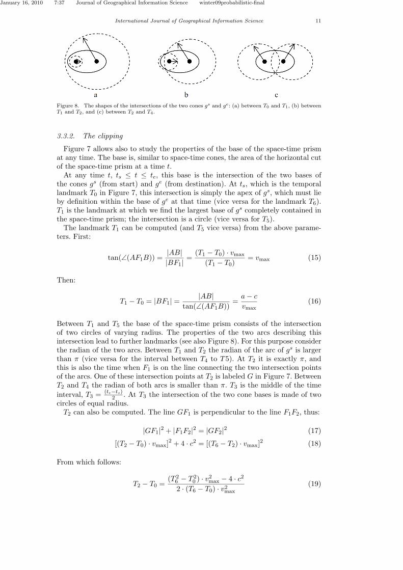
Figure 8. The shapes of the intersections of the two cones gs and ge: (a) between T0 and T1, (b) betweenT1 and T2, and (c) between T2 and T4.

3.3.2. The clipping

Figure 7 allows also to study the properties of the base of the space-time prismat any time. The base is, similar to space-time cones, the area of the horizontal cutof the space-time prism at a time t.

At any time t, ts ≤ t ≤ te, this base is the intersection of the two bases ofthe cones gs (from start) and ge (from destination). At ts, which is the temporallandmark T0 in Figure 7, this intersection is simply the apex of gs, which must lieby definition within the base of ge at that time (vice versa for the landmark T6).T1 is the landmark at which we find the largest base of gs completely contained inthe space-time prism; the intersection is a circle (vice versa for T5).

The landmark T1 can be computed (and T5 vice versa) from the above parame-ters. First:

tan(∠(AF1B)) =|AB||BF1| =

(T1 − T0) · vmax

(T1 − T0)= vmax (15)

Then:

T1 − T0 = |BF1| = |AB|tan(∠(AF1B))

=a− c

vmax(16)

Between T1 and T5 the base of the space-time prism consists of the intersectionof two circles of varying radius. The properties of the two arcs describing thisintersection lead to further landmarks (see also Figure 8). For this purpose considerthe radian of the two arcs. Between T1 and T2 the radian of the arc of gs is largerthan π (vice versa for the interval between T4 to T5). At T2 it is exactly π, andthis is also the time when F1 is on the line connecting the two intersection pointsof the arcs. One of these intersection points at T2 is labeled G in Figure 7. BetweenT2 and T4 the radian of both arcs is smaller than π. T3 is the middle of the timeinterval, T3 = (te−ts)

2 . At T3 the intersection of the two cone bases is made of twocircles of equal radius.

T2 can also be computed. The line GF1 is perpendicular to the line F1F2, thus:

|GF1|2 + |F1F2|2 = |GF2|2 (17)

[(T2 − T0) · vmax]2 + 4 · c2 = [(T6 − T2) · vmax]2 (18)

From which follows:

T2 − T0 =(T 2

6 − T 20 ) · v2

max − 4 · c2

2 · (T6 − T0) · v2max

(19)


12 Winter and Yin

Figure 9. The minimum bounding box of the clipping area at time t, with its parameters mx and my ina coordinate system aligned to λ.

3.3.3. The variance-covariance matrix Σ

While µ can be computed by Equation 10 at any time, what is still lacking isa model for the variance-covariance matrix Σ. Two aspects have to be considered.First, a relationship of the variances with the time budget of the traveler can bepostulated: the more time a traveler has to make detours the higher the variancesshould be. Accordingly, if the traveler has no time for detours, i.e., the potentialpath area has been degenerated to a line, the variances must be 0. This means, thevariances should be related to the size of the base of the space-time prism, i.e., theclipping areas considered above, which vary over time.

Secondly, the finite domain, the current base of the space-time prism at t, wouldrequire a normal distribution being clipped and normalized. But the knowledgethat the traveler is inside of the clipping area can also be used to choose appro-priate values for variances expressing this knowledge. The following considerationsguarantee that the probability to find the traveler within the clipping area is alwayslarger than 99.7% even without normalization, a figure where normalization caneven be neglected for most applications.

Let us assume that σx = σy; the observed fact that a traveler heads towardsa particular destination does not mean that we can assume anything about thedetours this traveler might take. For the same reason let us assume the covarianceσxy = 0, i.e., the movements in x and y are independent.

Now consider Figure 9, showing the clipping area at time t with its minimumbounding box oriented with F1F2, or in a coordinate system rotated by λ. Withinthis minimum bounding box two parameters can be introduced, mx and my. Thefirst parameter, mx, describes the shorter distance of µt to one of the sides ofthe minimum bounding box. Note, for this purpose, that µt is not always in thecenter of the minimum bounding box. Before T3 µt is in the center or right ofit, and afterwards it is in the center or left of it. For the situation in Figure 9(T0 < t < T3) this parameter can be described by mx = (vmax − v) · (t − T0).Accordingly, the second parameter, my, is the distance of µt to the top or bottomof the minimum box, which is symmetric. From the construction of the clippingarea it can be concluded that mx ≤ my at all times.

The figure also comes with a circle of radius mx: we do know now that such acircle must be always inside of the clipping area. Hence, by setting mx = 3σ theconsiderations above can be realized: the probability to find the traveler withinthe clipping area is always larger than 99.7%, and a normalization is not requiredfrom a practical perspective. Choosing any other σ would require normalization, sothis choice is not an arbitrary one but—in the end—derived from the possibilitiesof movement. With this choice, σ is also a function of time. Between T0 and T3

the variance follows from 3σ = (vmax − v) · (t − T0), and between T3 and T6 from



Figure 10. The standard deviation σ over time.

3σ = (vmax − v) · (T6 − t) (Figure 10). At T3 these values are equal, because atthat time µt is in the center of the clipping area. Figure 10 also shows the half ofheight and width of the minimum bounding box. Note that while my is equal tothe half of the height of the minimum bounding box, mx is not always equal tothe half of its width. For example, the half of the width of the minimum boundingbox is vmax(t− T0) between [T0, T1], then vmax(T1− T0) between [T1, T5], and thenvmax(T6 − t) between [T5, T6].

With the standard deviations and covariance at hand, Σt at time t and orientedinto the direction of the heading of the agent computes to:

Σt =(

cosλ − sinλsinλ cosλ

)(σ2

x 00 σ2

y

)

i

(cosλ sinλ− sinλ cosλ

)

=(

cos2 λσ2x + sin2 λσ2

y sinλ cosλσ2x − sinλ cosλσ2

y

sinλ cosλσ2x − sinλ cosλσ2

y sin2 λσ2x + cos2 λσ2

y

)

t

(20)

In this equation the rotation parallel to F1F2 is expressed by the eigen decompo-sition of Σt, with the eigenvalues σ2

x and σ2y , and the rotation matrix consisting of

the two eigenvectors of Σt.With these variables the bivariate normal distribution is determined completely.

Since Equation 11 was developed carefully as a function of time, it can be usedflexibly for any time t.

4. Example

This section illustrates the methodology introduced above. For this purpose themethodology was implemented in Matlab R2009a (Matlab is a product and regis-tered trademark from MathWorks). All figures in this section are computed withMatlab.

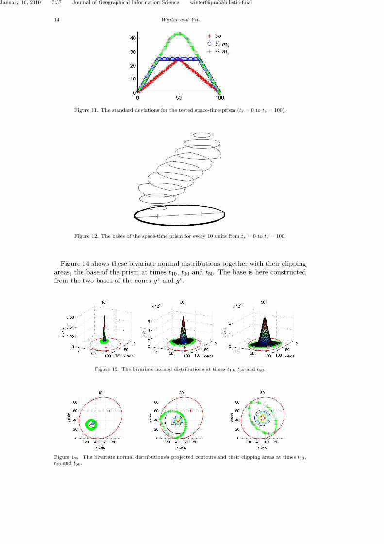
The bivariate normal distribution can represent the probability of an agent atany time. For the following illustrations we have chosen a start at (xs = 30, ys =30, ts = 0) and a destination at (xe = 70, ye = 60, te = 100). The maximal speedis vmax = 1. For these parameters the standard deviations show the behaviorpresented in Figure 11.

Figure 12 shows the bases of the space-time prism for every 10 units from ts = 0to te = 100. Theses bases will form the clipping areas for the bivariate normaldistributions.

Figure 13 shows the bivariate normal distributions, computed for t ={t10, t30, t50}, respectively. Additionally their contours are shown, projected intothe x − y−plane. Note that t50(= T3) is exactly the middle of the time intervalbetween start (ts) and end (te).


14 Winter and Yin

Figure 11. The standard deviations for the tested space-time prism (ts = 0 to te = 100).

Figure 12. The bases of the space-time prism for every 10 units from ts = 0 to te = 100.

Figure 14 shows these bivariate normal distributions together with their clippingareas, the base of the prism at times t10, t30 and t50. The base is here constructedfrom the two bases of the cones gs and ge.

Figure 13. The bivariate normal distributions at times t10, t30 and t50.

Figure 14. The bivariate normal distributions’s projected contours and their clipping areas at times t10,t30 and t50.



5. Conclusions

This paper extends a previous work on probabilistic space-time cones (Winter2009). It develops the mathematical foundations for modeling probabilistic space-time prisms, the time geography concept for movements between two known loca-tions in space and time. It shows that the pure fact of knowing an agent’s arrivalat a particular location at a particular time destroys the previous assumption ofuniform transition probabilities in a discrete space-time aquarium. Instead, theheading of the agent must be introduced as bias in a probabilistic model. This biasleads to a shift of the center of a probability distribution (towards the destination),but also to a time dependent variance-covariance matrix. The model is formulatedno longer as a discrete combinatorial one, as it was in Winter (2009), but as aclipped bivariate normal distribution. With probabilistic space-time cones (Winter2009) and probabilistic space-time prisms at hand, the set of space-time volumesin time geography is complete.

The model was successfully implemented in Matlab, which facilitates visual plau-sibility testing. Also, the resulting values of a clipped and normalized bivariatenormal distribution can now be used for probabilistic reasoning. With the proba-bility of an agent being at time t at a particular location questions can be answeredlike what is the probability of the agent to be in a specific area, or to have visiteda particular location by time t, or have met another agent. Developing a set ofqueries and the corresponding formula is part of the future work.

Another item of future work is the generalization of the presented model toa spatial and temporal discrete space-time aquarium. This generalization wouldbridge to the previous model of discrete space-time cones. Alternatively, the previ-ous model can now be formulated in a continuous manner. As both models assumeisotropic space, another extension of the presented model is required for anisotropicspace, such as network space.

The model presented in this paper is a purely theoretical one, and future workclearly needs to discuss its practical value or even its limitations in practical situ-ations. Looking at people’s activities, for example, their regularity would fit to thetheory: people leave their home on weekdays at 8am and arrive at work at 9am;the movements in between, collected over many days, may form a probabilisticspace-time prism. On the other hand we know that people’s wayfinding behavioris habitual, which violates a random walking model. For example, Gonzalez et al.(2008, p. 779) observe: “We find that, in contrast with the random trajectoriespredicted by the prevailing Levy flight and random walk models, human trajecto-ries show a high degree of temporal and spatial regularity, each individual beingcharacterized by a time independent characteristic travel distance and a significantprobability to return to a few highly frequented locations.” Such observations,based on the behavior of individuals, do not answer whether the sum of a largenumber of individuals—each of habitual behavior—would come closer to randombehavior patterns. It can also be argued that habitual wayfinding behavior devel-ops in street networks rather than open space. Accordingly, Helbing et al. (1997,2001), studying how people develop over time ‘trails’ in open spaces and findingthat these trails approximate shortest paths, provide again support for our model:physical trails emerge on paths chosen by a large number of people.

Gonzalez et al., referring to random walk models, cite studies of animal behav-ior (Viswanathan et al. 1996, Edwards et al. 2007). In fact, animal movements arecloser to random walks, also because of their comparatively unconstraint migration.In another example, (Laube et al. 2007) have studied the migratory behavior ofhoming pigeons from the same release site. Their data (e.g., their Figure 9) shows


16 REFERENCES

a nice similarity to the probability densities computed by our theoretic model.Similarly, one could expect to find in crowd movements similar patterns; for ex-ample, trajectories of a crowd crossing a street at a traffic light might lead to aprobabilistic space-time prism.

While more work needs to be done to empirically test the results across a broadrange of domains and applications, it has become clear that (a) the probability den-sity within space-time prisms is non-uniform, (b) a random walk model providesa sound and computationally feasible model to represent this density, further sup-porting time-geographic analysis, and (c) some empirical studies appear to cometo results supporting a random walk model.

Acknowledgements

The paper could be significantly improved by the comments of anonymous review-ers. Stephan Winter has been supported by grants of the Australian Academy ofScience and the Australian Research Council (DP0878119).

References

Balmer, M., Nagel, K. and Raney, B., 2004. Large Scale Multi-Agent Simulationsfor Transportation Applications. Journal of Intelligent Transport Systems, 8(4), 205–221.

Batty, M., 2003. Agent-Based Pedestrian Modelling. In: P.A. Longley and M. Batty,eds. Advanced Spatial Analysis. Redlands: ESRI Press, 81–106.

Bovy, P.H.L. and Stern, E., 1990. Route Choice: Wayfinding in Transport Networks.Dordrecht: Kluwer.

Camp, T., Boleng, J. and Davies, V., 2002. A Survey of Mobility Models for AdHoc Network Research. Wireless Communication and Mobile Computing, 2(5), 483–502.

Clementini, E. and Di Felice, P., 1996. An Algebraic Model for Spatial Objects withIndeterminate Boundaries. In: P.A. Burrough and A.U. Frank, eds. GeographicObjects with Indeterminate Boundaries., Vol. 2 of ESF GISDATA Taylor &Francis, 155–169.

Cohn, A.G. and Gotts, N.M., 1996. The ’Egg-Yolk’ Representation of Regions withIndeterminite Boundaries. In: P.A. Burrough and A.U. Frank, eds. GeographicObjects with Indeterminate Boundaries., Vol. 2 London: Taylor & Francis,171–187.

Edwards, A.M., Phillips, R.A., Watkins, N.W., Freeman, M.P., Murphy, E.J.,Afanasyev, V., Buldyrev, S.V., da Luz, M.G.E., Raposo, E.P., Stanley, H.E.and Viswanathan, G.M., 2007. Revisiting Levy Flight Search Patterns of Wan-dering Albatrosses, Bumblebees and Deer. Nature, 449 (25 October 2007),1044–1048.

Egenhofer, M.J. and Herring, J.R., Categorizing Binary Topological RelationshipsBetween Regions, Lines, and Points in Geographic Databases. , 1991. , Tech-nical report, Department of Surveying Engineering, University of Maine.

Gonzalez, M.C., Hidalgo, C.A. and Barabasi, A.L., 2008. Understanding IndividualHuman Mobility Patterns. Nature, 453 (5 June 2008), 779–782.

Guting, R.H. and Schneider, M., 2005. Moving Objects Databases. Amsterdam:Elsevier.

Hagerstrand, T., 1970. What about people in regional science?. Vol. 24, 7–21.


REFERENCES 17

Helbing, D., Keltsch, J. and Molnar, P., 1997. Modelling the Evolution of HumanTrail Systems. Nature, 388 (3 July 1997), 47–50.

Helbing, D., Molnar, P., Farkas, I.J. and Bolay, K., 2001. Self-Organzing PedestrianMovement. Environment and Planning B, 28 (3), 361–383.

Hoogendoorn, S.P. and Bovy, P.H.L., 2003. Traveller wayfinding in multimodaltransport networks. In: S. Timpf and M. Gould, eds. Euresco Conference onModelling for Wayfinding Services Bad Herrenalb: ESF.

Hornsby, K. and Egenhofer, M., 2002. Modeling Moving Objects over MultipleGranularities. Annals of Mathematics and Artificial Intelligence, 36 (1-2), 177–194.

Kwan, M.P., 2004. GIS Methods in Time-Geographic Research: Geocomputationand Geovisualization of Human Activity Patterns. Geografiska Annaler B, 86(4), 267–280.

Laube, P., Dennis, T., Forer, P. and Walker, M., 2007. Movement beyond theSnapshot: Dynamic Analysis of Geospatial Lifelines. Computers, Environmentand Urban Systems, 31 (5), 481–501.

Miller, H.J., 1991. Modeling Accessibility Using Space-Time Prism ConceptsWithin Geographical Information Systems. International Journal of Geograph-ical Information Science, 5 (3), 287–301.

Neutens, T., Witlox, F., van de Weghe, N. and de Maeyer, P., 2007a. Space-TimeOpportunities for Multiple Agents: A Constrained-Based Approach. Interna-tional Journal of Geographical Information Science, 21 (10), 1061–1076.

Neutens, T., Witlox, F., Van de Weghe, N. and De Maeyer, P., 2007b. HumanInteraction Spaces Under Uncertainty. Transportation Research Record, 2021,28–35.

Polya, G., 1921. Uber eine Aufgabe der Wahrscheinlichkeitsrechnung betreffenddie Irrfahrt im Straßennetz. Mathematische Annalen, 84, 149–160.

Randell, D.A., Cui, Z. and Cohn, A., 1992. A Spatial Logic Based on Regionsand Connection. In: R. Brachmann, H. Levesque and R. Reiter, eds. ThirdInternational Conference on the Principles of Knowledge Representation andReasoning. Los Altos, CA: Morgan-Kaufmann, 165–176.

Rubinstein, A., 1998. Modeling Bounded Rationality. Cambridge, Mass.: The MITPress.

Shannon, C.E. and Weaver, W., 1949. The Mathematical Theory of Communica-tion. Urbana, Illinois: The University of Illinois Press.

Shaw, S.L. and Yu, H., 2009. A GIS-Based Time-Geographic Approach of Study-ing Individual Activities and Interactions in a Hybrid PhysicalVirtual Space.Journal of Transport Geography, 17 (2), 141–149.

Tobler, W., 1970. A computer movie simulating urban growth in the Detroit region.Economic Geography, 46 (2), 234–240.

Viswanathan, G.M., Afanasyev, V., Buldyrev, S.V., Murphy, E.J., Prince, P.A. andStanley, H.E., 1996. Levy Flight Search Patterns of Wandering Albatrosses.Nature, 381 (30 May 1996), 413–415.

Winter, S., 2009. Towards a Probabilistic Time Geography. In: M. Mokbel,P. Scheuermann and W.G. Aref, eds. ACM SIGSPATIAL GIS 2009 ACMPress.

Winter, S. and Bittner, T., 2002. Hierarchical Topological Reasoning with VagueRegions. In: W. Shi, P. Fisher and M.F. Goodchild, eds. Spatial Data Quality.London: Taylor & Francis, 35–49.

Documents

RESEARCH PAPER Directed Movements in Probabilistic Time Geography · Time geography represents the reachable locations of this agent by a space-time cone, a right cone in x-y-t-space