Optimization Methods and SoftwareVol. 00, No. 00, Month 200x, 1–14

RESEARCH PAPER

COAL: A Generic Modelling and Prototyping Framework for

Convex Optimization Problems of Variational Image Analysis

Dirk Breitenreicher, Jan Lellmann, and Christoph Schnorr

Image and Pattern Analysis Group & HCI

Dept. of Mathematics and Computer Science, University of Heidelberg

breitenreicher,lellmann,schnoerr@math.uni-heidelberg.de(Received 00 Month 200x; in final form 00 Month 200x)

We present COAL, a flexible C++ framework for modelling and solving convex optimizationproblems in connection with variational problems of image analysis. COAL connects solverimplementations with specific models via an extensible set of properties, without enforcinga specific standard form. This allows to exploit the problem structure and to handle large-scale problems while supporting rapid prototyping and modifications of the model. Based onpredefined building blocks, a broad range of functionals encountered in image analysis can beimplemented and be reliably optimized using state-of-the-art algorithms, without the need toknow algorithmic details. We demonstrate the use of COAL on four representative variationalproblems of image analysis.

Keywords: image processing, variational modelling, convex optimization, sparse large-scaleprogramming

AMS Subject Classification: 90C25, 68U10, 62M40, 68T45

1. Introduction

Motivation and Related Work Variational approaches pervade the literature onimage processing and related aspects of machine learning and pattern recogni-tion [3, 17–19]. Such approaches are generally based on making models of observeddata and prior knowledge mathematically explicit through a joint optimizationcriterion, providing a sound basis for algorithm design. In particular, all kinds ofconvex optimization approaches have been established as major components ofvarious models in the recent years, since they can be solved globally optimal evenfor many large-scale problems, which allows to separate modelling questions fromoptimization issues.Choosing the best solver for a specific model is not straightforward however,

due to the vast amount of work published on both mathematical programmingand optimization-based image analysis, see e.g. [2, 4, 16, 18]. Available solvers andsoftware are often explicitly tailored to a specific problem formulation which raisessome issues:

• Commonly a self-contained description is lacking, hidden parameters are involvedor the solver is not thoroughly analysed;

• Improvements of the model may entail substantial modifications of the optimiza-tion process;

• Transferring methodological progress from one application area to another oneis a tedious task.

ISSN: 1055-6788 print/ISSN 1029-4937 onlinec⃝ 200x Taylor & FrancisDOI: 10.1080/03081080xxxxxxxxxhttp://www.informaworld.com

2

As a consequence, researchers interested in modelling advanced problems of imageanalysis require specific knowledge in algorithmic optimization in order to use,modify and combine models. This constitutes a considerable entry threshold whichmay drive them to abandon variational models altogether, and to resort to theheuristics they were originally trying to overcome.In contrast to such model-specific solvers, more generic optimization algorithms

and frameworks supporting higher-level languages provide greater flexibility andconcise representation, and thus are more suitable for model development [1, 11,15]. From the viewpoint of image analysis, however, there are significant drawbacks.

• Tools that provide an integrated modelling language such as AMPL1 [9],CVX [10], and YALMIP [14] transform the problem to an explicit, in-memoryintermediate standard form representation. Such representations do not scalevery well to the large-scale problems typical for low-level image analysis, such asvariational image labelling (Fig. 1) or video processing.

• Using solver packages directly, such as LAPACK, SeDuMi, CPLEX, MOSEK[15], TFOCS [1], or FastInf [11], one can usually avoid the explicit representationby using callback interfaces. This however requires a reformulation of the problemin a specific standard form, which is error-prone [14] and laborious to modify,introduces extra variables, and ignores specific problem structure.

• Higher-level languages such as MATLAB and Mathematica require a completere-implementation once a decision has been made to use research code outsidethe lab in a real application scenario. This again is an involved and error-proneprocess. Moreover, any modifications of the model beyond this stage requiresextensive modifications of the production code.

Therefore, we see a need for a framework that supports modelling of optimization-based approaches to image analysis and combines the speed and low memory foot-print of a lower-level language such as C++ with the ease of use, reusability, andconciseness of higher-level modelling languages.

Contribution We present the Convex Optimization Algorithms Library (COAL), aflexible algorithmic framework written in C++, that connects solvers – relying oncertain generic properties of the problem, such as differentiability, linearity, specificconstraint forms etc. – to models that exhibit these properties. COAL addressesthe issues raised above as follows:

• COAL neither enforces nor relies on an explicit representation. Instead, it sup-ports a compact problem implementation based on implicit representations wher-ever possible, similar to using callbacks. In particular, it efficiently handles large-scale problems.

• Using an extensible set of properties allows to formulate problems as close as pos-sible to their native mathematical formulation. This enables the solver to accessall information available about the problem, as long as a corresponding interfacehas been implemented. While COAL is not a complete modelling language, itallows to build complex problems from simple building blocks in a plug-and-playfashion, without transforming them to a standard form.

• COAL is implemented in C++ and relies on a fast lower-level linear algebrasubsystem. Overall performance is only slightly lower than for customized im-plementations. Therefore, a re-implementation can be avoided when moving frommodelling to production. Nevertheless, due to the modularity of the higher-level

1AMPL, CPLEX, Mathematica, MATLAB, and MOSEK are trademarks of their respective corporations.

3

Figure 1. Application of the proposed framework to exemplary multi-class labelling problems (Sect. 3.1).Top: histogram-based 3-class segmentation using total variation regularization where image regions charac-teristic for these classes have been marked by the user (top-left). The resulting partition of the input imageis shown top-right. Bottom: 16-class depth-from-stereo problem. A truncated linear distance regularizerwas used to infer the 16 different depth values in the scene (bottom-right). Solvers in COAL rely on fewgeneric properties of the objective functions available through interfaces, which makes them suitable for alarge class of models and facilitates the reuse of model components (Sect. 2).

optimization layer it is easy to add additional constraints, change the solver, oradd new functions if the problem specification changes.

We introduce COAL as a prototyping framework to support convex variationalmodelling of image analysis problems. However, similar problems commonly occurin many areas of image processing, computer vision and machine learning. There-fore the application of COAL in other fields is conceivable.Since COAL is implemented in C++, it can be easily used to extend most high-

level languages such as MATLAB or Mathematica, and scripting languages suchas Python.Rather than to replace existing dedicated solvers or to outperform them in terms

of efficiency, the primary motivation for our work is to provide a framework thatfacilitates the interaction between modelling and optimization, and supports pro-totyping, reproducibility of results, competitive evaluations, benchmarking, andranking of models.

Organization We outline COAL’s basic structure in Sect. 2 and show how we ad-dressed the issues discussed above. The practicability of COAL is demonstrated inSect. 3 on four prototypical problems from variational image analysis: multi-classlabelling, framelet-based inpainting, compressive sensing, and multi-view recon-struction. In Sect. 4 we provide a conclusion and point out availability of COAL.

4

Require: a signal y to be inpainted, a matrix A such as a gradient or framelet operator[5], a set of indices Ω of points to be inpainted.

1: g(x)← 12∥Ax∥22

2: h(x)← δ(x) =

0, if x(i) = y(i) for all i /∈ Ω,

+∞, otherwise.

3: f(x)← g(x) + h(x)4: Minimize f

Figure 2. Original specification of the pseudo-code required to solve the image inpainting problem(Sect. 3.2). Realizing the approach in COAL requires minimal problem-specific code (Fig. 3).

Require: y, A, Ω as in Fig. 2, a solver s.m = size(A, 1);n = size(A, 2);ConstantVector v(0.0, m);DenseVector l(n), u(n);

1: ...initialize l, u such that l(i) = u(i) = y(i) for i /∈ Ω and ±∞ otherwise...2: LeastSquaresFn g(A, v);3: BoxFn h(l, u);4: AutoSumFn f (&g, &h);5: s.Solve(&f);

Figure 3. Solving the image inpainting problem (Sect. 3.2) using COAL. With the exception of the tem-porary variables, the required C++ code corresponds almost line by line to the pseudo-code in Fig. 2.

2. Structure and Main Components of COAL

COAL consists of three main components:

• a template-based lower-level linear algebra subsystem providing the basic datastructures,

• a set of predefined building blocks, or functions, for formulating problems, and

• a set of solvers, each covering a broad range of problems, and relying on acommon set of function properties.

As outlined in the introduction, this structure aims at optimizing the trade-offbetween rapid prototyping and computational efficiency.We aim at providing a tool for quick modelling and optimization for non-expert

C/C++ users. In particular, the syntax should be non-cluttered and intuitive,with a similar ease of use as higher-level languages such as MATLAB. Thereforewe based the modelling part of the library on traditional object orientation usingvirtual inheritance, as opposed to more intricate template mechanisms.On the other hand, the performance-critical linear algebra subsystem uses a

template mechanism similar to FLENS [12]. The latter introduces additional com-plexity in the back end, but allows for efficient and concise expressions on the userside, and better compile-time optimizations.Both the high-level and low-level part encourage implicit, problem-specific rep-

resentations. Problems of moderate complexity such as image inpainting [18] (algo-rithm sketched in Fig. 2) can be realized in COAL in a straightforward way usingonly a few lines of code (Fig. 3).In the following, we provide a more detailed description of the three main parts

of the library: functions, solvers, and the linear algebra subsystem.

2.1. Functions

Many approaches for solving image analysis and computer vision problems arebased on balancing a performance criterion with prior knowledge by minimizing

5

Figure 4. An examplary inheritance and usage diagram for a simple differentiable objective function inthe COAL framework. Problems are uniformly represented as functions implementing certain interfaces,such as gradient- and function value computation while solvers use these interfaces in order to accessspecific function properties.

an objective function f(x) over some constraint set C of feasible solutions:

min f(x) s.t. x ∈ C . (1)

While the subdivision into objective and constraint set is intuitive, it is often notunique and leads to redundant code and data structures for solving equivalent butdifferently formulated problems.Instead, we adopt the unifying representation often encountered in the optimiza-

tion literature, where constraints x ∈ C are not explicitly represented, but ratherspecified as part of the objective: minimize f(x) = g(x) + δC(x), where δC is theindicator function,

δC(x) =

0, x ∈ C ,

+∞, x ∈ C . (2)

Consequently, in COAL every problem is represented as a function f : Rn 7→R ∪ +∞, whose minimum should be computed. Each function class inheritsfrom the Function base class and provides several interfaces that correspond toproperties of the underlying mathematical functions.

Interfaces All knowledge about the specific problem is introduced by means ofinterfaces: for instance, functions may be composed of a sum of simpler functions(ISum), differentiable functions may provide a method to evaluate the gradient(IGradient), or the user may be able to explicitly compute proximal/backwardsteps [7] (IBackwardStep).Using this approach, we reduce the interaction between solvers and functions to a

small set of interfaces (sketched in Fig. 4). This increases interoperability betweensolvers and functions, and maximizes code reuse, since functions that implement acertain set of interfaces can automatically be used by a wide range of solvers.Some properties, such as differentiability, are usually fixed at compile time, while

others can dynamically change at run time depending on the input data: for ex-ample, linear regression problems of the form f(x) = 1

2∥Ax − b∥22 can be triviallysolved if the matrix A, coming from the specific problem instance, has diagonal ortriangular form, while the general case is much more involved.These concepts are supported by a run-time interface mechanism. Properties are

accessed using expressions such as intf<IGradient>(f)->Gradient(x). Using thesame mechanism, functions may provide reformulations in terms of standard formssuch as linear programs, second-order cone programs, or saddle-point problems(Sect. 2.2) for solvers that rely on these representations.

6

Custom Functions and Properties When implementing a custom function, theuser generally has to reflect about its structure and to decide which interfacescan be supported. For common cases such as the sum of simpler functions withknown properties, COAL provides composite function adapters such as AutoSumFn,that automatically infer many properties from properties of the contained parts.Interfaces can be freely added on the function and solver side as required. Forinstance, the interface to evaluate LeastSquaresFn is defined by the source code:

1: class LeastSquaresFn : public Function, protected IEvaluatable 2: ...3: virtual double Evaluate(const ConstVectorRef& x) const 4: // code for evaluating the least squares function5: 6: DefineInterfaces_(7: Interface_(IEvaluatable, this);8: );9: ;

Subsequently, each instance f of a LeastSquaresFn can be evaluated via the prop-erties mechanism intf<IEvaluatable>(f)->Evaluate(x).

2.2. Solvers

In view of the previous discussion, we postulate that solvers should be formulatedin their most general form. As an example, consider a simple projected-gradientsolver minimizing a function g over some convex constraint set C, hence minimizingf = g + δC , in the COAL framework.While this could be implemented using a “project onto set” interface for the

constraints, it is better to regard the projection operation as a specific instanceof a proximal/backward step on δC : by designing the solver to just rely on themore general backward step operation, it becomes applicable for the far largerclass of problems of the form f = g+h, where h can be any function on which thebackward step can be performed. This generalized method is known as forward-backward splitting in the operator splitting framework [7, 8], and is obtained at noadditional cost when implementing the scheme in COAL.Below we provide the code for an exemplary forward-backward solver. The vari-

ables control, step, point are the class internal control structure, a step-sizeparameter, and a storage container:

1: class ForwardBackward : public Solver 2: ...3: virtual Status Solve(const Function* f) 4: const ISum::FunctionArray* fct = &intf<const ISum>(f)->Functions();5: const IGradient* grad = intf<const IGradient>((*fct)[0]);6: const IBackwardStep* bw = intf<const IBackwardStep>((*fct)[1]);7:

8: int k = 1;9: do

10: axpyi(-step, grad->Gradient(*point), *point);11: copy(bw->BackwardStep(*point, step), *point);12:

13: control->Accept("k", k);14: ++k;15: while (!control->Terminate());16:

17: return status.SetCode(Status::Solved);18: 19: virtual ConstVectorRef Solution() const

7

20: return *point;21: 22: virtual void SetParameter(const string& s, const parameter_type& p) 23: ... // set solver parameters such as step-size or control24: 25: ;

Currently Supported Solvers In the current implementation we settled on twogeneric problem classes. First, since many generic convex solvers rely on a certainconic program form (cf. [2]), we implemented the quadratic form with second-order cone constraints. It includes second-order cone programs (SOCP) and linearprograms (LP) as special cases, and assumes the structure

minx

x⊤Qx+ q⊤x

s.t. Ax ≤ b, Cx = d, l ≤ x ≤ u, x ∈ K ,(3)

where K denotes a set of second-order cones. In addition, we provide an interfacefor the saddle-point formulation

minx∈C

maxv∈Dh(x) + ⟨v,Ax⟩ − g(v) , (4)

where h(x) and g(v) are convex functions in the primal and dual domain. Thisformulation has the advantage of explicitly formalizing the dual variables whilekeeping the number of slack variables minimal.In the back end, COAL currently includes three prototypical solvers: an interface

to the commercial – but free for academic use – MOSEK package [15], Nesterov’sefficient first-order optimization scheme [16], and a simple but powerful primal-dualsolver [6], which generalizes the previously presented forward-backward scheme [7,8]. Including new algorithms and solvers in future versions is straight-forward, bycreating a class which derives from Solver and implements the required interfacefunctions Solve, Solution, and SetParameter.

2.3. Linear Algebra Subsystem

In order to cope with large-scale real-world data, the lower-level matrix/vector datastructures and elementary operations have to be sufficiently fast. COAL builds ona sub-library that provides a basic set of data structures, that can also be usedindependently of the modelling part.For maximum efficiency, we rely on a C++ template mechanism inspired by

the FLENS library [12]. Costly virtual function calls are completely avoided. Newmatrix and vector types are introduced by defining a corresponding class, andspecializing functions that compute basic operations on these matrices or vectors,such as element access of matrix-vector products.COAL includes basic types for dense matrices based on BLAS, sparse matrices,

and several special types such as constant, diagonal, and block matrices.The library strongly encourages the introduction of new types as required, in

particular in cases where matrices have a specific or sparse structure or can be im-plemented without explicitly allocating storage. Third-party data structures canbe easily interfaced by providing a wrapper. COAL includes such a wrapper forworking transparently with the MATLAB “mex” matrix type in MATLAB exten-sions.

8

The approach is fully scalable in the sense that getting new types up and runningrequires the user to implement only very few functions to access the size and theelements of the matrix. If required, performance can be gradually increased byproviding fast substitutes for the generic fallbacks, such as for vector addition ormatrix-vector multiplication.For instance, a ScaledIdentityMatrix of size s × s could be implemented as

follows:

1: class ScaledIdentityMatrix : public ConstViewBase<ScaledIdentityMatrix>2: 3: ...4: double c; mindex dim;5:

6: DiagonalMatrix (const double c_in, index s)7: : c(c_in), dim(s, s) 8: const mindex& size() const 9: return dim;

10: 11: double operator()(index i) const 12: return ((i-1)%dim(1)==(i-1)/dim(1)) ? c : 0.0;13: 14: double operator()(index i, index j) const 15: return (i==j) ? c : 0.0;16: 17: bool contains (const double* location) const 18: return false;19: 20: ;

All matrix-vector operations are encapsulated in templated kernel classes, whichcan be specialized to provide faster implementations. As an example, the follow-ing code speeds up the generic matrix-vector inner product x⊤Qy for Q of typeScaledIdentityMatrix by specializing inner_kernel:

1: template<typename TX, typename TY>2: struct inner_kernel::implementation<TX, ScaledIdentityMatrix, TY>3: 4: double operator()(const inner_kernel&, const TX& x,5: const ScaledIdentityMatrix& Q, const TY& y) 6: return Q.c * dot(x,y);7: 8: ;

Here the COAL function dot(·,·) implements the standard dot product for twovectors.

3. Case Studies

In this section, we consider different applications from the field of computer vision,and show how they can be solved using COAL. For each of the problems, we statethe model, provide the code for constructing the model and calling the solver, andshow some numerical results.

3.1. Image Labelling

Model Many problems in image analysis and computer vision can be reduced tothe basic problem of assigning, to each point x in the image, one of l discretelabels 1, . . . , l. This is typically achieved by minimizing an energy consisting of a

9

local data fidelity term and a regularization term that enforces spatial coherence.Applications include segmentation, stereo matching, photo montage, and manymore [18].For many interesting regularizers, such as the total variation (TV), the multiclass

labelling problem can be relaxed to a variational problem of the form

minx∈C⟨x, s⟩+Ψ(Lx) . (5)

Here the primal constraint set C is a product of unit simplices. The data termis described by the vector s, while the regularization is encoded in the matrixL (usually exhibiting gradient-like structure), and in the positively homogeneous,lower semi-continuous function Ψ.Using Fenchel duality, the problem can be naturally reformulated as a saddle-

point problem [13],

minx∈C

maxv∈D⟨x, s⟩+ ⟨Lx, v⟩ , (6)

where the structure of Ψ is encoded in the dual constraint set D. This class of prob-lems includes linear programming relaxations of classical pairwise Markov randomfields, as well as more recent higher-order labelling and lifting approaches [6, 13].

Implementation Implementing and optimizing (6) in COAL reduces to specifyingthe matrix L, implementing functions that represent the primal and dual constraintsets, and providing a method to project onto these sets. The linear terms arehandled out-of-the-box. The actual C++ code for building the model and passingit to the solver is as follows:

1: LinearFn dataterm(im);2: TVFn reg(dims, D);3: SimplexFn constraints(dims);4: AutoSumFn primalPart(&dataterm, &constraints);5: AutoPrimalDualForm problem(&primalPart, &reg);6:

7: FastPrimalDual s;8: s.SetParameter("tau_primal",step);9: s.SetParameter("tau_dual",step);

10: s.SetParameter("start",ConstantVector(1.0/dims.Components(), dims.NTotal()));11: s.Solve(&problem);12: copy(s.Solution(), y)

where im represents the image, step encodes an appropriate step-size parameterand dims is a user defined struct containing additional information such as numberof variables or number of components, to simplify notations.Although the gradient matrix D could be provided as a standard dense matrix,

this would be very inefficient in terms of memory. Instead, letting A define thedesired properties of the regularizer, we use an implicit representation in terms ofa block matrix, where each block contains a gradient operator:

1: BlockMatrix D;2: for (int i = 1; i <= dims.Components; ++i) 3: BlockMatrix* row = new BlockMatrix();4: for (int j = 1; j <= dims.Components(); ++j) 5: GradientMatrix* g = new GradientMatrix(s1, s2,6: GradientMatrix::Neumann, A(i,j));7: row->Append(*g, 2);8:

10

9: D.Append(*row, 1);10:

Constructing D in this manner fully retains its sparse structure, thereby decreasingmemory requirements and increasing performance.

Results Figure 1 shows exemplary applications to 3-class image segmentationbased on colour histograms with total variation regularization, and depth-from-stereo using 16 depth labels and truncated linear regularization.Although the applications are conceptually different, once the data term s has

been computed and the matrix L has been assembled, the models can be solvedusing the same code base, and one of the available solvers [6, 16].

3.2. Image Inpainting

Model Another prototypical problem in computer vision is the image inpaintingproblem [5, 18]. For a given signal y with missing data at pixels specified by a setof indices Ω, a “likely” signal x should be reconstructed such that for i /∈ Ω, xi = yi(Fig. 2). This can be cast into the constrained least squares problem

minx

1

2∥Ax∥22 s.t. xi = yi, ∀i /∈ Ω , (7)

where y defines the image to be reconstructed, Ω specifies the inpainting region andA refers to a matrix, such as a framelet matrix, that introduces prior knowledge [5].

Implementation To realize the problem in COAL (Fig. 3), the user has to providethe problem structure, i.e., to specify l, u such that the information encoded inΩ can be written as a box constraint l ≤ x ≤ u, where l(i) = u(i) for all i /∈ Ωand l(i) = −∞, u(i) = +∞ otherwise, as well as the filter matrix A, either asexplicit values or implicitly in terms of an algorithm for computing the matrix-vector product. Due to its large-scale nature, representing A explicitly is typicallyinfeasible [5], therefore we chose an implicit representation. Given an input imageim and output image y, as well as a lower and upper bound l, u that encode theinpainting region, the procedure to solve the inpainting problem is as follows:

1: CubicFrameletMatrix A (size(im,1), size(im,2));2:

3: BoxFn constraint (l, u);4: LeastSquaresFn lsq (A, ConstantVector(0.0, size(A,1)));5: AutoSumFn problem (&lsq, &constraint);6:

7: Nesterov s;8: s.SetParameter("start", ConstantVector(0.0, size(A,2)));9: s.Solve(&problem);

10: copy(s.Solution(), y);

The final code is very close to the original algorithm in Fig. 3.

Results For solving (7), we use the efficient first-order algorithm from [16]. Be-sides specifying the stopping criterion, no additional problem-specific code is re-quired, since the problem is decomposed automatically such that the solver canbe applied (see Fig. 5). The final result for the 256 × 256 input image, with a

11

Figure 5. Prototypical use of the proposed software framework for the problem of image inpainting(Sect. 3.2). We used a simplified framelet approach [5] without sub-sampling. The underlying mathe-matical problem of recovering the white regions (left) can be modelled efficiently using COAL (Fig. 3).Variants such as replacing the least squares objective (middle) by a robust Huber kernel (right) can beevaluated by changing a single line of code.

524288 × 65536 matrix A (cf. [5]), is determined in a few minutes using a singlecore Pentium 4 3.00 GHz machine.A particular benefit of using COAL is the flexibility during the prototyping

stage. As the least squares objective (7) tends to be sensitive to sharp edges,robust distance measures such as the Huber kernel [5] have been proposed. Suchmodifications can be evaluated easily, in this case by changing line 4: in the abovesource code to HuberFn g(A, v), where v = ConstantVector(0.0, size(A,1)).

3.3. Multi-View 3D Reconstruction

Model We now consider the problem of multi-view reconstruction. Given a setof projected 2D measurements along with corresponding camera parameters, theobjective is to reconstruct the three-dimensional shape of the object (Fig. 6). Math-ematically, this problem can be modelled using an ℓ1 objective with second-ordercone constraints [20, Eqn. (5)] as

minx∥Dx∥1 , s.t. Ax = b, l ≤ x, x ∈ C , (8)

where D,A refers to a matrix and b, l are vectors. C denotes a set of cones specifiedby a set of indices I ∈ Nm,n such that x ∈ C if ∀ i = 1, . . .m, xIi,1 ≥ (

∑nk=2 x

2Ii,k

)1

2 ,

cf. [20] and the references therein.

Implementation Starting from this formulation, the user can combine the individ-ual parts in COAL directly using the provided functions, in an analogue fashion toFig. 3. The corresponding source code is given by

1: AffineEqFn constraint (A, b);2: L1Fn l1 (D, ConstantVector(0.0, size(D,1)));3: SecondOrderConeFn cone (cone_index, size(A,2));4: BoxFn box (l, BoxFn::Lower);5: AutoSumFn problem (&l1, &constraint);6: problem.Append(&box);7: problem.Append(&cone);8: AutoConicForm conic_form (&problem);9:

10: Mosek msk;11: msk.Solve(&conic_form);

12

Figure 6. Application of COAL to the multi-view 3D reconstruction problem [20]. Given a set of sampleviews (prototypical views depicted on the left, middle), the objective is to reconstruct the corresponding3D point cloud (right, Sect. 3.3). The problem can be prototyped and solved in COAL with only a fewlines of code.

where cone_index represents C by means of a set of indices for each constraint.We point out that it is not necessary to manually introduce slack variables for

the ℓ1 objective in order to arrive at formulation (3), as is the case when usingstandard solvers such as [15]. Instead, COAL handles the introduction of slackvariables automatically (Line 8:), since AutoSumFn is capable of merging the con-tained functions into a single SOCP suitable for solvers such as MOSEK. Thismakes the error-prone task of manual problem reformulation obsolete.

Results Although the library is only moderately tuned in its current form, the final≈ 5000 3D points (Fig. 6), causing D to be a diagonal 146513 × 146513 matrixand A ∈ R98592×146513 being sparse with 410800 non-zero elements, are delivered inless than one minute when using the MOSEK interface. This is comparable to thetime reported in [20] where a Douglas-Rachford like splitting algorithm was usedto optimize different reformulations of (8). In order to further increase runtimeperformance, exploiting problem specific structures (e.g., fill-in patterns of sparsematrices) and parallel computation could be considered.

3.4. Sparse Representation

Model Mathematically related to the image inpainting problem is the sparse rep-resentation problem, where the goal is to select a small set of atoms from a largedictionary a1, . . . , an ∈ Rm such that a given signal f ∈ Rm is well-approximatedby their weighted sum, where typically m ≪ n. We consider this application tocompare the runtime and memory requirements of COAL to a problem-specificnative C++ implementation.The sparse representation problem is often solved by considering the mathemat-

ical problem

minx∈Rn

1

2∥Ax− f∥22 + µ∥x∥1 , (9)

where A = (a1, . . . , an), ∥ · ∥1 is the non-smooth ℓ-1 norm measuring sparsity ofthe argument and µ refers to a user control parameter.

Implementation To solve (9), we consider the primal-dual algorithm [6]. GivenA, f, µ, the optimization problem can be implemented in COAL as follows:

13

100 200 300 400 500m

0.005

0.010

0.050

0.100

0.500

1.000

sec

cu stom ized im p l.

COAL im p l.

100 200 300 400 500m

1

10

100

1000

kB

cu stom ized im p l.

COAL im p l.

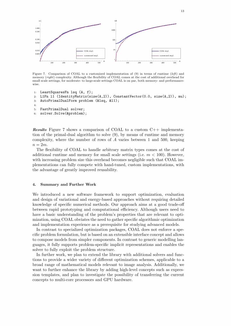
Figure 7. Comparison of COAL to a customized implementation of (9) in terms of runtime (left) andmemory (right) complexity. Although the flexibility of COAL comes at the cost of additional overhead forsmall scale settings, for moderate- to large-scale settings COAL is on par, both memory- and performance-wise.

1: LeastSquaresFn lsq (A, f);2: L1Fn l1 (IdentityMatrix(size(A,2)), ConstantVector(0.0, size(A,2)), mu);3: AutoPrimalDualForm problem (&lsq, &l1);4:

5: FastPrimalDual solver;6: solver.Solve(&problem);

Results Figure 7 shows a comparison of COAL to a custom C++ implementa-tion of the primal-dual algorithm to solve (9), by means of runtime and memorycomplexity, where the number of rows of A varies between 1 and 500, keepingn = 2m.The flexibility of COAL to handle arbitrary matrix types comes at the cost of

additional runtime and memory for small scale settings (i.e. m < 100). However,with increasing problem size this overhead becomes negligible such that COAL im-plementations can fully compete with hand-tuned, custom implementations, withthe advantage of greatly improved reusability.

4. Summary and Further Work

We introduced a new software framework to support optimization, evaluationand design of variational and energy-based approaches without requiring detailedknowledge of specific numerical methods. Our approach aims at a good trade-offbetween rapid prototyping and computational efficiency. Although users need tohave a basic understanding of the problem’s properties that are relevant to opti-mization, using COAL obviates the need to gather specific algorithmic optimizationand implementation experience as a prerequisite for studying advanced models.In contrast to specialized optimization packages, COAL does not enforce a spe-

cific problem formulation, but is based on an extensible interface concept and allowsto compose models from simpler components. In contrast to generic modelling lan-guages, it fully supports problem-specific implicit representations and enables thesolver to fully exploit the problem structure.In further work, we plan to extend the library with additional solvers and func-

tions to provide a wider variety of different optimization schemes, applicable to abroad range of mathematical models relevant to image analysis. Additionally, wewant to further enhance the library by adding high-level concepts such as expres-sion templates, and plan to investigate the possibility of transferring the currentconcepts to multi-core processors and GPU hardware.

14 REFERENCES

As the theory and computational approaches to image analysis consolidate, therewill be an increasing need for higher-level software environments supporting theinvestigation of increasingly complex systems. With COAL we aim to take a timelystep in this direction.COAL will be made publicly available under an open source license on our web-

site1 in the near future.

References

[1] Becker, S., Candes, E. J., and Grant, M. Templates for convex cone problems with applicationsto sparse signal recovery. Math. Programming Comput. 3, 3 (2011), 165–218.

[2] Ben-Tal, A., and Nemirovski, A. Lectures on Modern Convex Optimization. MPS-SIAM Series onOptimization, 2001.

[3] Bennett, K., and Parrado-Hernandez, E. The interplay of optimization and machine learningresearch. J. Mach. Learning Res. 7 (2006), 1265–1281.

[4] Boykov, Y., and Funka-Lea, G. Graph cuts and efficient N-D image segmentation. Int. J. Com-put. Vision 70, 2 (2006), 109–131.

[5] Cai, J., Chan, R., and Shen, Z. A framelet-based image inpainting algorithm. Applied and Com-putational Harmonic Analysis 24 (2008), 131–149.

[6] Chambolle, A., and Pock, T. A first-order primal-dual algorithm for convex problems with appli-cations to imaging. J. Math. Imaging Vis. 40, 1 (2011), 120–145.

[7] Combettes, P. L., and Pesquet, J.-C. Proximal splitting methods in signal processing. In Fixed-Point Algorithms for Inverse Problems in Science and Engineering. Springer, New York, 2010.

[8] Combettes, P. L., and Wajs, V. R. Signal recovery by proximal forward-backward splitting. Mul-tiscale Model. Simul. 4, 4 (2005), 1168–1200.

[9] Fourer, R., Gay, D. M., and Kernighan, B. W. AMPL: A Modeling Language for MathematicalProgramming. Duxbury Press, 2002.

[10] Grant, M., and Boyd, S. CVX: Matlab software for disciplined convex programming.http://cvxr.com/cvx, 2010.

[11] Jaimovich, A., Meshi, O., and Elidan, G. FastInf: An efficient approximate inference library.J. Mach. Learning Res. 11 (2010), 1733–1736.

[12] Lehn, M. FLENS – a flexible library for efficient numerical solutions in C++.http://flens.sourceforge.net.

[13] Lellmann, J., Becker, F., and Schnorr, C. Convex optimization for multi-class image labelingwith a novel family of total variation based regularizers. In Int. Conf. Comput. Vision (2009).

[14] Lofberg, J. YALMIP: A toolbox for modeling and optimization in MATLAB. In Proc. CACSDConf. (2004).

[15] The MOSEK optimization package. www.mosek.com.[16] Nesterov, Y. Smooth minimization of non-smooth functions. Math. Prog. 103, 1 (2004), 127–152.[17] NIPS 3rd international workshop on optimization for machine learning, 2010.

http://opt.kyb.tuebingen.mpg.de.[18] Paragios, N., Chen, Y., and Faugeras, O. D., Eds. Handbook of Mathematical Models in Computer

Vision. Springer, 2005.[19] Wainwright, M., and Jordan, M. Graphical models, exponential families, and variational inference.

Found. Trends Mach. Learning 1, 1-2 (2008), 1–305.[20] Zach, C., and Pollefeys, M. Practical methods for convex multi-view reconstruction. In Proc. Eu-

rop. Conf. Comput. Vision (2010).

1http://ipa.iwr.uni-heidelberg.de