Embed Size (px)
Citation preview
Journal of theBrazilian Computer Society
Saraiva et al. Journal of the Brazilian ComputerSociety (2017) 23:11 DOI 10.1186/s13173-017-0060-0
RESEARCH Open Access
Incorporating decision maker’spreferences in a multi-objective approach forthe software release planningRaphael Saraiva1* , Allysson Allex Araújo2, Altino Dantas3, Italo Yeltsin1 and Jerffeson Souza1
Abstract
Background: Release planning (RP) is one of the most complex and relevant activities in the iterative andincremental software development, because it addresses all decisions associated with the selection and assignmentof requirements to releases. There are many approaches in which RP is formalized as an optimization problem. In thiscontext, search-based software engineering (SBSE) deals with the application of search techniques to solve complexproblems of software engineering. Since RP is a wicked problem with a large focus on human intuition, the decisionmaker’s (DM) opinion is a relevant issue to be considered when solving release planning problem. Thus, weemphasize the importance in gathering the DM’s preferences to guide the optimization process through searchspace area of his/her interests.
Methods: Typically, RP is modelled as a multi-objective problem by considering to maximize overall clientssatisfaction and minimize project risk. In this paper, we extend this notion and consider DM’s preferences as anadditional objective. The DM defines a set of preferences about the requirements allocation which is stored in apreference base responsible for influencing the search process. The approach was validated through an empiricalstudy, which consists of two different experiments, respectively identified as (a) automatic experiment and (b)participant-based experiment. Basically, the former aims to analyze the approach using different search-basedalgorithms (NSGA-II, MOCell, IBEA, and SPEA-II), over artificial and real-world instances, whereas the latter aims atevaluating the use of the proposal in a real scenario composed of human evaluations.
Results: The automatic experiment points out that NSGA-II obtained overall superiority in two of the three datasetsinvestigated, positioning itself as a superior search technique for scenarios with few number of requirements andpreferences, while IBEA showed to be better for larger ones (with more requirements and preferences). Regarding theparticipant-based experiment, it was found that two thirds of the participants evaluated the preference-basedsolution better than the non-preference-based one.
Conclusions: The results suggest that it is feasible to investigate the approach in a real-world scenario. In addition,we made available a prototype tool in order to incorporate the human’s preferences about the requirementsallocation into the solution of release planning.
Keywords: Release planning, Multi-objective optimization, Human preferences, Search-based software engineering
*Correspondence: [email protected] University of Ceará, Dr. Silas Munguba Avenue, 1700 Fortaleza, CE, BrazilFull list of author information is available at the end of the article
© The Author(s). 2017 Open Access This article is distributed under the terms of the Creative Commons Attribution 4.0International License (http://creativecommons.org/licenses/by/4.0/), which permits unrestricted use, distribution, andreproduction in any medium, provided you give appropriate credit to the original author(s) and the source, provide a link to theCreative Commons license, and indicate if changes were made.
Saraiva et al. Journal of the Brazilian Computer Society (2017) 23:11 Page 2 of 19
IntroductionThe incremental and iterative software life cycle is basedon the idea of developing an initial system implementa-tion and evolving it through several releases in a cyclic way[1]. Release planning (RP) addresses all decisions relatedto the requirements selection and assignment to a consec-utive sequence of releases [2]. As stated by Ruhe and Saliu[3], good RP practices ensure that the software is builton providing the maximum business value by offering thebest possible blend of features in the right sequence ofreleases. On the other hand, poor RP decisions can resultin the following: (i) unsatisfied customers; (ii) release plansthat are unlikely to be delivered within a given schedule,quality, and effort specifications; and (iii) release plansthat do not offer the best business values.Given the cognitive effort involved in dealing with RP,
defining a “suitable” set of releases is inherently chal-lenging. As “suitable,” we may consider that it properlydeals with variables that present complex relations suchas stakeholders’ preferences, technical constraints, limitedresources, and subjective business aspects. In addition,this process can be time-consuming, requiring one to ana-lyze an exhaustive list of possible combinations, whichtend to be extremely large if the number of requirements isgreat. There are a number of existing approaches that arebased on the belief that RP can be formalized as an opti-mization problem and widely explored by Search-basedsoftware engineering (SBSE) as well. In summary, SBSEproposes to apply search techniques to solve complexproblems of software engineering [4].However, RP is a wicked problem with a large focus on
human intuition, communication, and human capabilities.For a wicked problem, it is not clear what the problem isand, therefore, what the solution is [3]. Additionally, turn-ing the decision maker’s (DM) feelings as a useful part ofthe resolution process may help avoid some resistance orlittle confidence in the final result [5]. Instead of just pro-viding a simple weight factor for each requirement, forexample, we emphasized the importance of providing arefined mechanism to efficiently capture the human pref-erences and, consequently, guide the search process. Thismechanism must intuitively enable the DM to expresshis/her preferences in a broad scope, focusing the timein essential subjective aspects. As subjective aspects, werefer to the questions that are complex to define withouthuman interaction, especially implicit information. Forinstance, the DM may want to allocate specific featuresin different releases, establish precedence relations orcoupling relations between features according to his/hersubjective knowledge.In other words, we have to integrate the computational
intelligence power with the human expertise to obtainmore realistic and acceptable solutions for some wickedproblems. In general, two main benefits arise from this
perspective, which are to provide meaningful insights tothe DM and increase the human engagement [6]. As dis-cussed by Marculescu et al. [7], intuitive interaction withdomain specialists is a key factor in industrial applicabil-ity, since it makes the system more usable and more easilyaccepted in an industrial setting. Despite the promisingoutlook, the definition regarding the type and how thepreferences are exploited by optimization algorithms is arelevant challenge and has attracted attention in recentyears.Recently, the SBSE approaches based on this assumption
have been discussed under the requirements engineeringcontext. Araújo et al. [8] propose an architecture for thenext release problem (NRP) based on the usage of an inter-active genetic algorithm alongside a machine learningmodel. In that work, the preferences are gathered througha subjective mark provided by the DM to each solution,while a machine learning model learns his/her evaluationprofile. After a certain number of subjective evaluations,the machine learning model replaces the DM and evalu-ates the remainder of the solutions. While considering theNRP, Ferreira et al. [9] propose an interactive ant colonyoptimization, where the DM is asked to specify whichrequirements he/she expects to be present or not in thenext release. While these previous studies are focused onthe requirements selection, Tonella, Susi, and Palma [10]present an interactive approach to the requirements prior-itization. The information elicited from the user consistsof a pairwise comparison between the requirements thatare ordered differently in equally scored prioritization.Regarding planning more than one release, an initial
proposal of the present work was described by Dantaset al. [11]. It was designed as a single-objective model,which allows the DM to express different types of pref-erences considering the requirements allocation. Suchpreferences are stored in the preference base, in whichthe main purpose is to influence the search process. Itwas verified in the performed experiment that there wasan unavoidable trade-off between the problem’s metrics(score and risk) and the subjective preference. This con-flict occurs because sometimes the solutions have to losesome value in score or risk to satisfy the DM’s preferences.To extend Dantas et al.’s [11] proposal, an earlier ver-
sion of this work is investigated to deal with the DMpreferences as another objective to be maximized in amulti-objective model [12]. Notwithstanding, the pro-posed approach included a strategy called the referencepoint method [13] to mitigate the usual cognitive effortof selecting a solution from the Pareto front. Empiri-cal results were able to demonstrate the feasibility of theapproach in an artificial environment.Therefore, this paper significantly extends the previous
work in twomajor aspects: (a) besides increasing the auto-matic experiment through two more search techniques,
Saraiva et al. Journal of the Brazilian Computer Society (2017) 23:11 Page 3 of 19
one large artificial dataset, and additional results, we alsoconduct a participant-based experiment to observe thebehavior of the approach in a real-world context and (b)a prototype tool was developed and made available toenable a novel way to incorporate the human preferencesduring the release planning. The primary contributions ofthis paper can be summarized as follows:
• Experimental analyses considering both simulatedand real human evaluations
• The presentation of a prototype tool for the releaseplanning process
The remainder of this paper is organized as follows. The“Background” section presents the approach background,whereas the “Mathematical formulation” section detailsthe mathematical model. The “Empirical study” sectiondiscusses the empirical study, and finally, the “Concludingremarks” section presents some conclusions and direc-tions for future works.
BackgroundSearch-based software engineeringSoftware engineers often face problems associated withbalancing competing constraints, trade-off between con-cerns, and requirement imprecision. Software engineeringis typically concerned with a near optimal solution orthose that fall within a specified acceptable tolerance [14].In these situations, automated optimization techniquesare natural candidates. Thus, search-based software engi-neering (SBSE) seeks to reformulate software engineeringproblems as search problems. A search problem is one inwhich optimal or near optimal solutions are sought in asearch space of candidate solutions [4].As highlighted by Harman [15], there are only two key
ingredients for the application of search-based optimiza-tion to software engineering problems:
• The choice of the problem representation amenableto symbolic manipulation
• The definition of the fitness function to characterizewhat is considered to be a good solution
SBSE has been applied to many fields within the gen-eral area of software engineering, such as requirements
engineering [16], software design [17], and testing [18].A wide range of different optimization and search tech-niques have been used by SBSE, with evolutionary algo-rithms (EAs) being the most popular ones [19]. EAsare generic and stochastic population-based algorithmsthat are inspired by biological and natural evolution con-cepts, such as reproduction, mutation, recombination,and selection [20]. In this work, we evaluated four differ-ent EAs, namely NSGA-II [21], MOCell [22], IBEA [23],and SPEA-II [24].
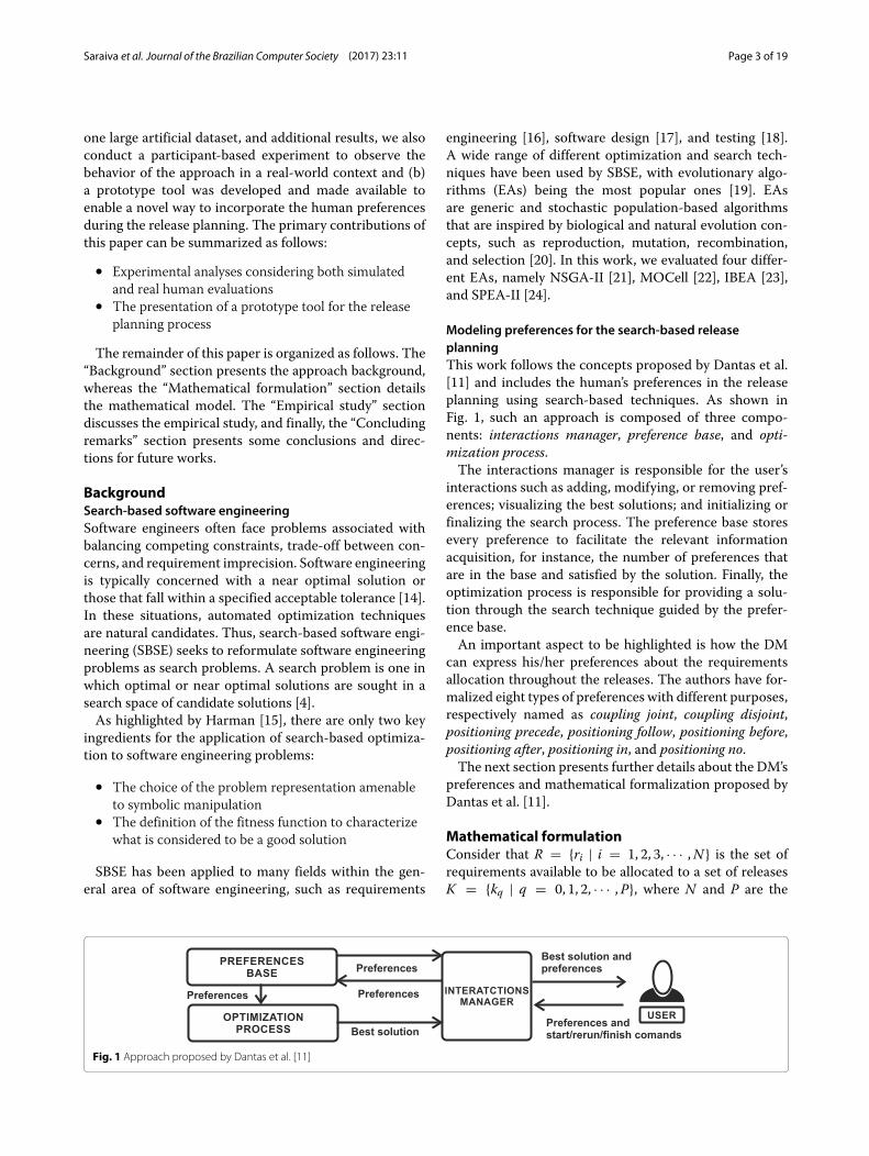
Modeling preferences for the search-based releaseplanningThis work follows the concepts proposed by Dantas et al.[11] and includes the human’s preferences in the releaseplanning using search-based techniques. As shown inFig. 1, such an approach is composed of three compo-nents: interactions manager, preference base, and opti-mization process.The interactions manager is responsible for the user’s
interactions such as adding, modifying, or removing pref-erences; visualizing the best solutions; and initializing orfinalizing the search process. The preference base storesevery preference to facilitate the relevant informationacquisition, for instance, the number of preferences thatare in the base and satisfied by the solution. Finally, theoptimization process is responsible for providing a solu-tion through the search technique guided by the prefer-ence base.An important aspect to be highlighted is how the DM
can express his/her preferences about the requirementsallocation throughout the releases. The authors have for-malized eight types of preferences with different purposes,respectively named as coupling joint, coupling disjoint,positioning precede, positioning follow, positioning before,positioning after, positioning in, and positioning no.The next section presents further details about the DM’s
preferences and mathematical formalization proposed byDantas et al. [11].
Mathematical formulationConsider that R = {ri | i = 1, 2, 3, · · · ,N} is the set ofrequirements available to be allocated to a set of releasesK = {kq | q = 0, 1, 2, · · · ,P}, where N and P are the
Fig. 1 Approach proposed by Dantas et al. [11]
Saraiva et al. Journal of the Brazilian Computer Society (2017) 23:11 Page 4 of 19
number of requirements and releases, respectively. Thevector S = {x1, x2, · · · , xN } represents the solution, wherexi ∈ {0, 1, 2, · · · ,P} stores the release kq in which therequirement ri is allocated, and xi = 0 means that sucha requirement was not allocated. In addition, considerC = {cj | j = 1, 2, 3, · · · ,M}, where M is the numberof clients and each client cj has a weight wj to estimatehis/her importance to the company that develops thesoftware. The function Value(i), which represents howvaluable requirement ri is, returns the weighted sum of thescores that each client cj assigned to the requirement ri asfollows:
Value(i) =M∑
j=1wj × Score(cj, ri), (1)
where Score(cj, ri) quantifies the perceived importancethat a client cj associates with a requirement ri assigninga value ranging from 0 (no importance) to 10 (the high-est importance). Thus, the value of the objective related tothe overall client satisfaction is given by
Satisfaction(S) =N∑
i=1(P − xi + 1) × Value(i) × yi, (2)
where yi ∈ {0, 1} is a decision variable that has a valueof 1 if the requirement ri is allocated to some release and0 otherwise. This binary variable is necessary to avoida requirement ri being computed when it is not allo-cated. As suggested by Baker et al. [25], the clients areusually satisfied when the requirements they most pre-fer are implemented. Therefore, (P − xi + 1) is used forSatisfaction(S) to become higher when the requirementswith a high Value(i) are allocated in the first releases, i.e,maximizing the overall clients’ satisfaction.In addition to maximizing the client’s satisfaction,
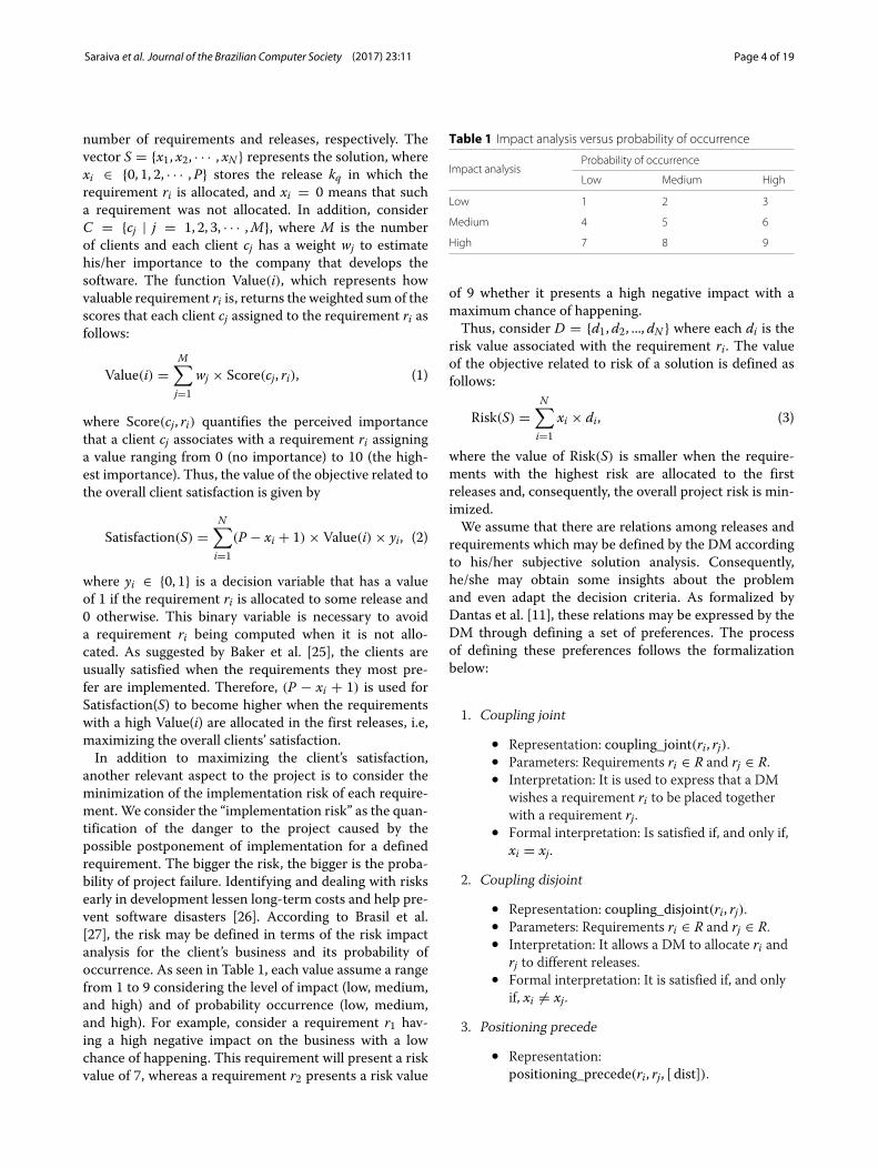
another relevant aspect to the project is to consider theminimization of the implementation risk of each require-ment. We consider the “implementation risk” as the quan-tification of the danger to the project caused by thepossible postponement of implementation for a definedrequirement. The bigger the risk, the bigger is the proba-bility of project failure. Identifying and dealing with risksearly in development lessen long-term costs and help pre-vent software disasters [26]. According to Brasil et al.[27], the risk may be defined in terms of the risk impactanalysis for the client’s business and its probability ofoccurrence. As seen in Table 1, each value assume a rangefrom 1 to 9 considering the level of impact (low, medium,and high) and of probability occurrence (low, medium,and high). For example, consider a requirement r1 hav-ing a high negative impact on the business with a lowchance of happening. This requirement will present a riskvalue of 7, whereas a requirement r2 presents a risk value
Table 1 Impact analysis versus probability of occurrence
Impact analysisProbability of occurrence
Low Medium High
Low 1 2 3
Medium 4 5 6
High 7 8 9
of 9 whether it presents a high negative impact with amaximum chance of happening.Thus, consider D = {d1, d2, ..., dN } where each di is the
risk value associated with the requirement ri. The valueof the objective related to risk of a solution is defined asfollows:
Risk(S) =N∑
i=1xi × di, (3)
where the value of Risk(S) is smaller when the require-ments with the highest risk are allocated to the firstreleases and, consequently, the overall project risk is min-imized.We assume that there are relations among releases and
requirements which may be defined by the DM accordingto his/her subjective solution analysis. Consequently,he/she may obtain some insights about the problemand even adapt the decision criteria. As formalized byDantas et al. [11], these relations may be expressed by theDM through defining a set of preferences. The processof defining these preferences follows the formalizationbelow:
1. Coupling joint
• Representation: coupling_joint(ri, rj).• Parameters: Requirements ri ∈ R and rj ∈ R.• Interpretation: It is used to express that a DM
wishes a requirement ri to be placed togetherwith a requirement rj.
• Formal interpretation: Is satisfied if, and only if,xi = xj.
2. Coupling disjoint
• Representation: coupling_disjoint(ri, rj).• Parameters: Requirements ri ∈ R and rj ∈ R.• Interpretation: It allows a DM to allocate ri and
rj to different releases.• Formal interpretation: It is satisfied if, and only
if, xi �= xj.
3. Positioning precede
• Representation:positioning_precede(ri, rj, [ dist]).
Saraiva et al. Journal of the Brazilian Computer Society (2017) 23:11 Page 5 of 19
• Parameters: Requirements ri ∈ R, rj ∈ R and aminimum distance between the requirements,with a value always greater than zero.
• Interpretation: It enables a DM to specify that arequirement ri must be positioned at least distreleases before a requirement rj.
• Formal interpretation: It is satisfied if at leastone of the following conditions is fulfilled:
(xi, xj �= 0 and xj − xi ≥ dist) OR(xi �= 0 and xj = 0).
4. Positioning follow
• Representation:positioning_follow(ri, rj, [ dist]).
• Parameters: Requirements ri ∈ R, rj ∈ R and aminimum distance between the requirements,with a value always greater than zero.
• Interpretation: It expresses that a requirement rimust be positioned at least dist releases afteranother requirement rj.
• Formal interpretation: It is satisfied if at leastone of the following conditions is met:
(xi, xj �= 0 and xi − xj ≥ dist) OR(xi = 0 and xj �= 0).
5. Positioning before
• Representation: positioning_before(ri, kq).• Parameters: Requirement ri ∈ R and a release kq.• Interpretation: It defines that a requirement ri
may be assigned to any release before a specificrelease kq.
• Formal interpretation: It is satisfied when thefollowing conditions are met:
(xi �= 0) AND (kq − xi ≥ 1).
6. Positioning after
• Representation: positioning_after(ri, kq).• Parameters: Requirement ri ∈ R and a release kq.• Interpretation: It defines that a requirement ri
may be assigned to any release after a specificrelease kq.
• Formal interpretation: It is satisfied when thefollowing conditions are met:
(xi �= 0) AND (xi − kq ≥ 1).
7. Positioning in
• Representation: positioning_in(ri, kq).• Parameters: Requirement ri ∈ R and a release kq.• Interpretation: It allows the DM to place a
requirement ri in a specific release kq.• Formal interpretation: It is satisfied if, and only
if, xi = kq.
8. Positioning no
• Representation: positioning_no(ri, kq).• Parameters: Requirement ri ∈ R and a release kq.• Interpretation: It defines that a requirement ri
should not be assigned in the release kq.• Formal interpretation: It is satisfied if, and only
if, xi �= kq.
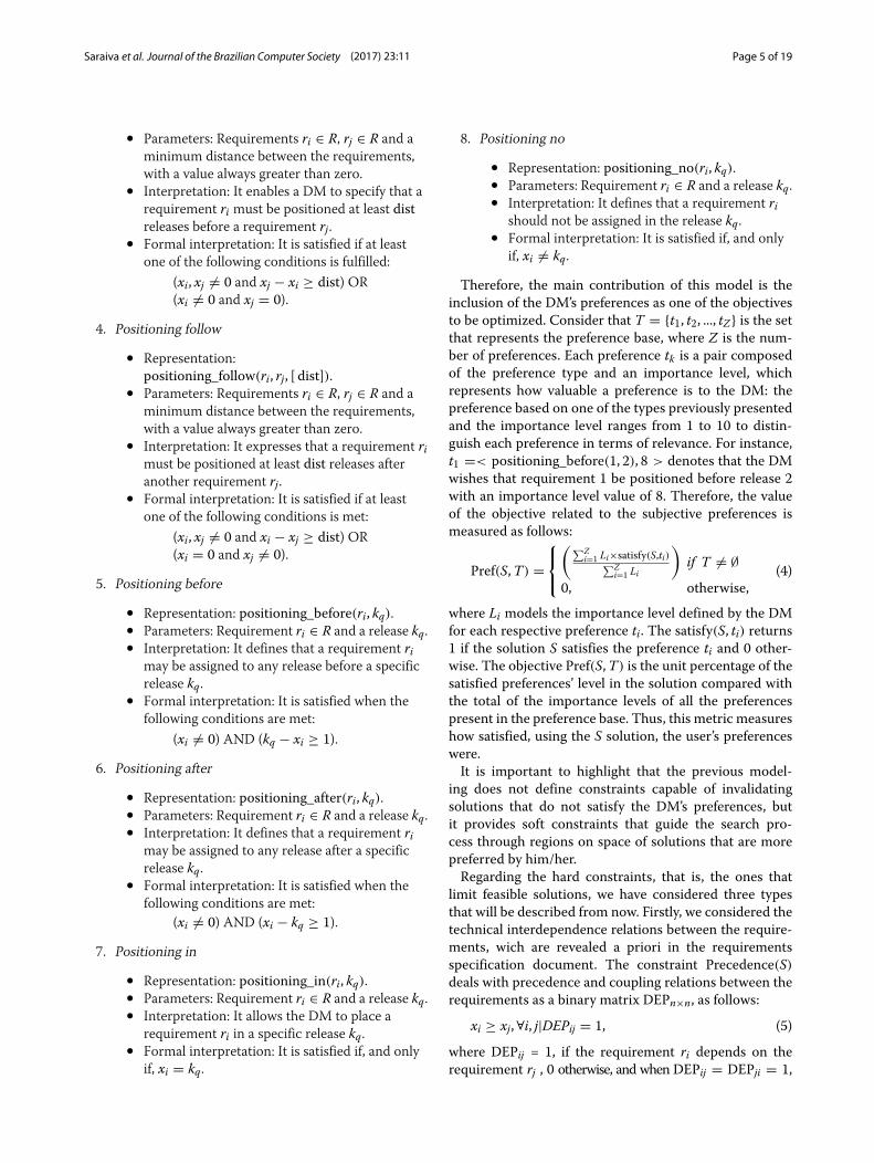
Therefore, the main contribution of this model is theinclusion of the DM’s preferences as one of the objectivesto be optimized. Consider that T = {t1, t2, ..., tZ} is the setthat represents the preference base, where Z is the num-ber of preferences. Each preference tk is a pair composedof the preference type and an importance level, whichrepresents how valuable a preference is to the DM: thepreference based on one of the types previously presentedand the importance level ranges from 1 to 10 to distin-guish each preference in terms of relevance. For instance,t1 =< positioning_before(1, 2), 8 > denotes that the DMwishes that requirement 1 be positioned before release 2with an importance level value of 8. Therefore, the valueof the objective related to the subjective preferences ismeasured as follows:
Pref(S,T) =⎧⎨
⎩
(∑Zi=1 Li×satisfy(S,ti)∑Z
i=1 Li
)if T �= ∅
0, otherwise,(4)
where Li models the importance level defined by the DMfor each respective preference ti. The satisfy(S, ti) returns1 if the solution S satisfies the preference ti and 0 other-wise. The objective Pref(S,T) is the unit percentage of thesatisfied preferences’ level in the solution compared withthe total of the importance levels of all the preferencespresent in the preference base. Thus, this metric measureshow satisfied, using the S solution, the user’s preferenceswere.It is important to highlight that the previous model-
ing does not define constraints capable of invalidatingsolutions that do not satisfy the DM’s preferences, butit provides soft constraints that guide the search pro-cess through regions on space of solutions that are morepreferred by him/her.Regarding the hard constraints, that is, the ones that
limit feasible solutions, we have considered three typesthat will be described from now. Firstly, we considered thetechnical interdependence relations between the require-ments, wich are revealed a priori in the requirementsspecification document. The constraint Precedence(S)deals with precedence and coupling relations between therequirements as a binary matrix DEPn×n, as follows:
xi ≥ xj,∀i, j|DEPij = 1, (5)
where DEPij = 1, if the requirement ri depends on therequirement rj , 0 otherwise, and when DEPij = DEPji = 1,
Saraiva et al. Journal of the Brazilian Computer Society (2017) 23:11 Page 6 of 19
the requirements ri and rj must be implemented in thesame release. The remainder of the matrix is filled with 0,indicating that there is no relation between the require-ments and no technical limitation on their position assign-ment.Furthermore, the Budget(S) constraint treats the
resources available for each release. Thus, considering thateach requirement ri has a costi and each release kp has abudget value bp, this constraint guarantees that the sum ofthe costs of all requirements allocated to each release doesnot exceed the correspondent budget:
N∑
i=1inRelease(xi, kj) × costi < bj,
∀j ∈ {1, 2, 3, . . . ,P},inRelease(xi, j) =
{1, if xi = j0, otherwise.
Finally, the constraint ReqForRelease(S) guarantees thateach release j has at least one allocated requirement. Thisconstraint is described below:
N∑
i=1inRelease(xi, j) > 0. (6)
Therefore, our multi-objective formulation of therelease planning consists of:
maximize Satisfaction(S),maximize Pref(S,T),minimize Risk(S),subject to: 1)Precedence(S),
2)ReqForRelease(S),3)Budget(S).
(7)
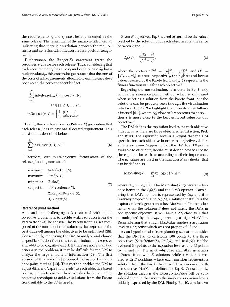
Reference point methodAn usual and challenging task associated with multi-objective problems is to decide which solution from thePareto front will be chosen. The Pareto front is a set com-posed of the non-dominated solutions that represents thebest trade-off among the objectives to be optimized [28].Consequently, requesting the DM to analyze and choosea specific solution from this set can induce an excessiveand additional cognitive effort. If there are more than twocriteria in the problem, it may be difficult for the DM toanalyze the large amount of information [29]. The firstversion of this work [12] proposed the use of the refer-ence point method [13]. This method enables the DM toadjust different “aspiration levels” to each objective basedon his/her preferences. These weights help the multi-objective technique to achieve solutions from the Paretofront suitable to the DM’s needs.
GivenG objectives, Eq. 8 is used to normalize the valuesreached by the solution S for each objective i in the rangebetween 0 and 1.
�fi(S) = fi(S) − o∗i
onadi − o∗i, (8)
where the vectors Onad = {onad1 , . . . , onadG
}and O∗ ={
o∗1, . . . , o∗
G}express, respectively, the highest and lowest
values reached by the Pareto front and fi(S) represents thefitness function value for each objective i.Regarding the normalization, it is done in Eq. 8 only
within the reference point method, which is only usedwhen selecting a solution from the Pareto front, but thesolutions can be properly seen through the visualizationinterface (Fig. 4). We highlight the normalization followsa interval [0,1], where �fi close to 0 represents that a solu-tion S is more close to the best achieved value for thisobjective i.The DMdefines the aspiration level ai for each objective
i. In our case, there are three objectives (Satisfaction, Pref,and Risk). The aspiration level is a weight that the DMspecifies for each objective in order to subjectively differ-entiate each one. Supposing that the DM has 100 pointsavailable to distribute, he/she must decide how to allocatethese points for each ai according to their importance.The ai values are used in the function MaxValue(S) thatcan be defined as
MaxValue(S) = maxi=1,...,G
�fi(S) × �qi, (9)
where �qi = ai/100. The MaxValue(S) generates a bal-ance between the �fi(S) and the DM’s opinion. Consid-ering that DM’s opinion is represented by �qi and it isinversely proportional to �fi(S), a solution that fulfills theaspiration levels generates a low MaxValue. On the otherhand, when the solution S does not satisfy the DM’s inone specific objective, it will have a �fi close to 1 thatis multiplied by the �qi, generating a high MaxValue.Remembering that a high MaxValue implies a aspirationlevel to a objective which was not properly fulfilled.As an hypothetical release planning scenario, consider
that the DM has to distribute 100 points to the threeobjectives (Satisfaction(S), Pref(S), and Risk(S)). He/sheassigned 34 points to the aspiration level a1 and 33 pointsto a2 and a3. The multi-objective algorithm generatesa Pareto front with E solutions, while a vector is cre-ated with E positions where each position represents asolution from the Pareto front, which is associated witha respective MaxValue defined by Eq. 9. Consequently,the solution that has the lowest MaxValue will be con-sidered the one that meets the majority aspiration levelsinitially expressed by the DM. Finally, Eq. 10, also known
Saraiva et al. Journal of the Brazilian Computer Society (2017) 23:11 Page 7 of 19
as the scalarizing function, represents the solution searchprocess from the Pareto front:
minimize MaxValue(S),subject to: S ∈ E.
(10)
Empirical studyThe following sections present all of the details regardingthe empirical study in which we followed some empiricalsoftware engineering guidelines, such as data collectionprocedure and quantitative results presentation [30, 31].First, the experimental design specifications as well asresearch questions are presented. Then, the analysis anddiscussion of the achieved results are explained. Finally,the threats that may affect the validity of the experimentsare emphasized.
Experimental designThe empirical study was divided into two different exper-iments, (a) automatic experiment and (b) participant-based experiment. Essentially, the first one aims to analyzethe approach using different search-based algorithms,over artificial and real-world instances, while the secondone aims to evaluate the use of the proposal in a realscenario composed of human evaluations.
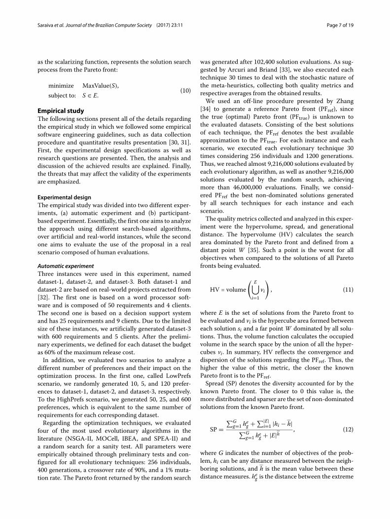
Automatic experimentThree instances were used in this experiment, nameddataset-1, dataset-2, and dataset-3. Both dataset-1 anddataset-2 are based on real-world projects extracted from[32]. The first one is based on a word processor soft-ware and is composed of 50 requirements and 4 clients.The second one is based on a decision support systemand has 25 requirements and 9 clients. Due to the limitedsize of these instances, we artificially generated dataset-3with 600 requirements and 5 clients. After the prelimi-nary experiments, we defined for each dataset the budgetas 60% of the maximum release cost.In addition, we evaluated two scenarios to analyze a
different number of preferences and their impact on theoptimization process. In the first one, called LowPrefsscenario, we randomly generated 10, 5, and 120 prefer-ences to dataset-1, dataset-2, and dataset-3, respectively.To the HighPrefs scenario, we generated 50, 25, and 600preferences, which is equivalent to the same number ofrequirements for each corresponding dataset.Regarding the optimization techniques, we evaluated
four of the most used evolutionary algorithms in theliterature (NSGA-II, MOCell, IBEA, and SPEA-II) anda random search for a sanity test. All parameters wereempirically obtained through preliminary tests and con-figured for all evolutionary techniques: 256 individuals,400 generations, a crossover rate of 90%, and a 1% muta-tion rate. The Pareto front returned by the random search
was generated after 102,400 solution evaluations. As sug-gested by Arcuri and Briand [33], we also executed eachtechnique 30 times to deal with the stochastic nature ofthe meta-heuristics, collecting both quality metrics andrespective averages from the obtained results.We used an off-line procedure presented by Zhang
[34] to generate a reference Pareto front (PFref), sincethe true (optimal) Pareto front (PFtrue) is unknown tothe evaluated datasets. Consisting of the best solutionsof each technique, the PFref denotes the best availableapproximation to the PFtrue. For each instance and eachscenario, we executed each evolutionary technique 30times considering 256 individuals and 1200 generations.Thus, we reached almost 9,216,000 solutions evaluated byeach evolutionary algorithm, as well as another 9,216,000solutions evaluated by the random search, achievingmore than 46,000,000 evaluations. Finally, we consid-ered PFref the best non-dominated solutions generatedby all search techniques for each instance and eachscenario.The quality metrics collected and analyzed in this exper-
iment were the hypervolume, spread, and generationaldistance. The hypervolume (HV) calculates the searcharea dominated by the Pareto front and defined from adistant point W [35]. Such a point is the worst for allobjectives when compared to the solutions of all Paretofronts being evaluated.
HV = volume( E⋃
i=1vi
), (11)
where E is the set of solutions from the Pareto front tobe evaluated and vi is the hypercube area formed betweeneach solution si and a far point W dominated by all solu-tions. Thus, the volume function calculates the occupiedvolume in the search space by the union of all the hyper-cubes vi. In summary, HV reflects the convergence anddispersion of the solutions regarding the PFref. Thus, thehigher the value of this metric, the closer the knownPareto front is to the PFref.Spread (SP) denotes the diversity accounted for by the
known Pareto front. The closer to 0 this value is, themore distributed and sparser are the set of non-dominatedsolutions from the known Pareto front.
SP =∑G
g=1 heg + ∑|E|i=1 |hi − h|
∑Gg=1 heg + |E|h , (12)
where G indicates the number of objectives of the prob-lem, hi can be any distance measured between the neigh-boring solutions, and h is the mean value between thesedistance measures. heg is the distance between the extreme
Saraiva et al. Journal of the Brazilian Computer Society (2017) 23:11 Page 8 of 19
solutions of PFref and E, corresponding to the gth objec-tive function.Finally, the generational distance (GD) contributes to
calculating the distance between the known Pareto frontobtained by the optimization technique and the PFref.
GD =√∑E
i=1 euc2in
, (13)
where the value of euci is the smallest Euclidean distanceof a solution i ∈ E to a solution from PFref.
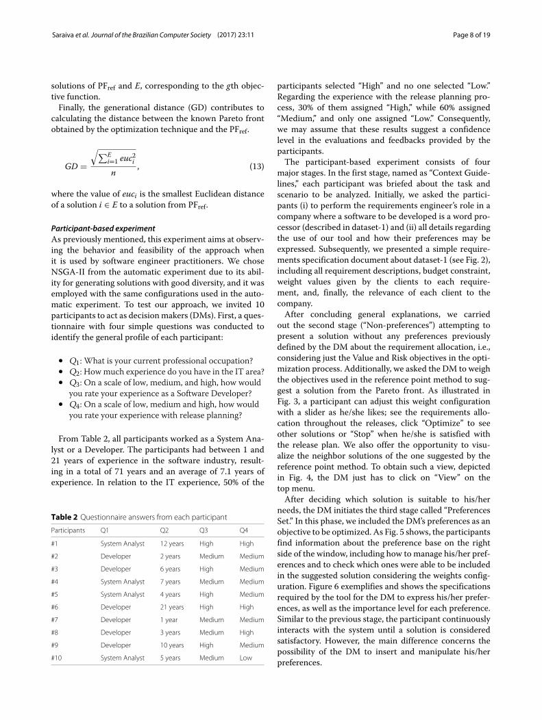
Participant-based experimentAs previously mentioned, this experiment aims at observ-ing the behavior and feasibility of the approach whenit is used by software engineer practitioners. We choseNSGA-II from the automatic experiment due to its abil-ity for generating solutions with good diversity, and it wasemployed with the same configurations used in the auto-matic experiment. To test our approach, we invited 10participants to act as decisionmakers (DMs). First, a ques-tionnaire with four simple questions was conducted toidentify the general profile of each participant:
• Q1: What is your current professional occupation?• Q2: Howmuch experience do you have in the IT area?• Q3: On a scale of low, medium, and high, how would
you rate your experience as a Software Developer?• Q4: On a scale of low, medium and high, how would
you rate your experience with release planning?
From Table 2, all participants worked as a System Ana-lyst or a Developer. The participants had between 1 and21 years of experience in the software industry, result-ing in a total of 71 years and an average of 7.1 years ofexperience. In relation to the IT experience, 50% of the
Table 2 Questionnaire answers from each participant
Participants Q1 Q2 Q3 Q4
#1 System Analyst 12 years High High
#2 Developer 2 years Medium Medium
#3 Developer 6 years High Medium
#4 System Analyst 7 years Medium Medium
#5 System Analyst 4 years High Medium
#6 Developer 21 years High High
#7 Developer 1 year Medium Medium
#8 Developer 3 years Medium High
#9 Developer 10 years High Medium
#10 System Analyst 5 years Medium Low
participants selected “High” and no one selected “Low.”Regarding the experience with the release planning pro-cess, 30% of them assigned “High,” while 60% assigned“Medium,” and only one assigned “Low.” Consequently,we may assume that these results suggest a confidencelevel in the evaluations and feedbacks provided by theparticipants.The participant-based experiment consists of four
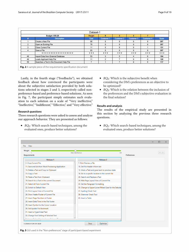
major stages. In the first stage, named as “Context Guide-lines,” each participant was briefed about the task andscenario to be analyzed. Initially, we asked the partici-pants (i) to perform the requirements engineer’s role in acompany where a software to be developed is a word pro-cessor (described in dataset-1) and (ii) all details regardingthe use of our tool and how their preferences may beexpressed. Subsequently, we presented a simple require-ments specification document about dataset-1 (see Fig. 2),including all requirement descriptions, budget constraint,weight values given by the clients to each require-ment, and, finally, the relevance of each client to thecompany.After concluding general explanations, we carried
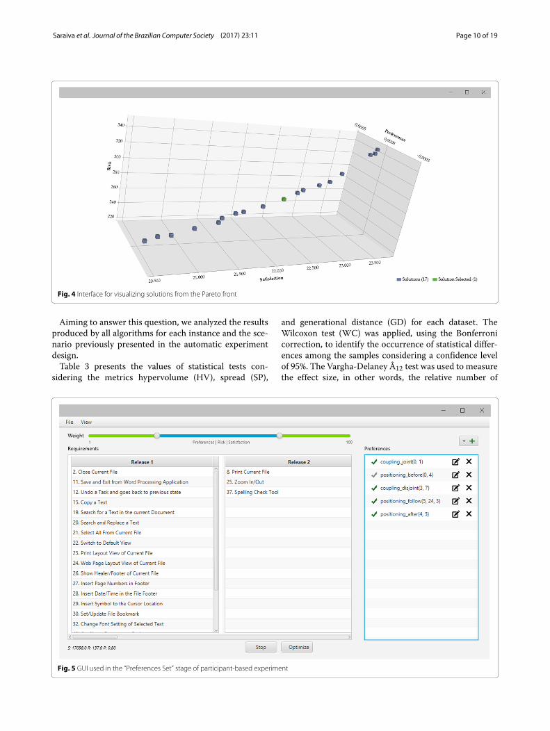
out the second stage (“Non-preferences”) attempting topresent a solution without any preferences previouslydefined by the DM about the requirement allocation, i.e.,considering just the Value and Risk objectives in the opti-mization process. Additionally, we asked the DM to weighthe objectives used in the reference point method to sug-gest a solution from the Pareto front. As illustrated inFig. 3, a participant can adjust this weight configurationwith a slider as he/she likes; see the requirements allo-cation throughout the releases, click “Optimize” to seeother solutions or “Stop” when he/she is satisfied withthe release plan. We also offer the opportunity to visu-alize the neighbor solutions of the one suggested by thereference point method. To obtain such a view, depictedin Fig. 4, the DM just has to click on “View” on thetop menu.After deciding which solution is suitable to his/her
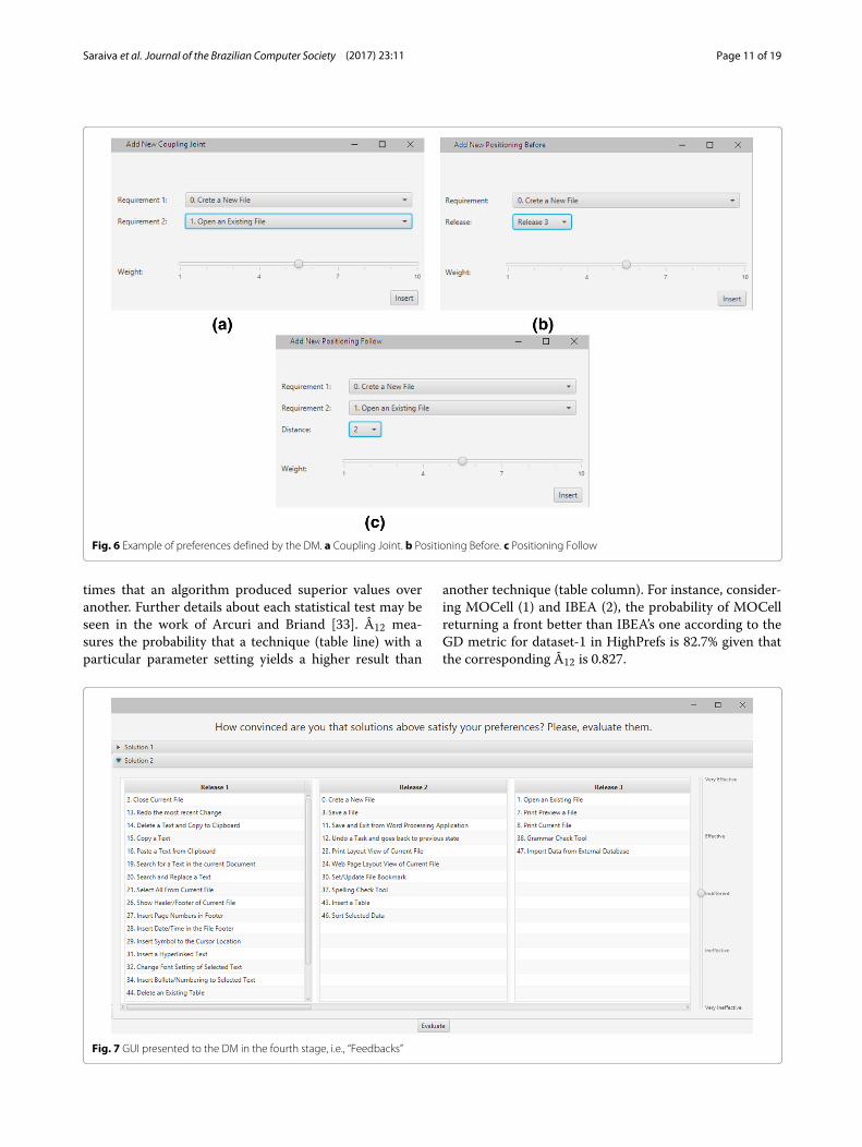
needs, the DM initiates the third stage called “PreferencesSet.” In this phase, we included the DM’s preferences as anobjective to be optimized. As Fig. 5 shows, the participantsfind information about the preference base on the rightside of the window, including how to manage his/her pref-erences and to check which ones were able to be includedin the suggested solution considering the weights config-uration. Figure 6 exemplifies and shows the specificationsrequired by the tool for the DM to express his/her prefer-ences, as well as the importance level for each preference.Similar to the previous stage, the participant continuouslyinteracts with the system until a solution is consideredsatisfactory. However, the main difference concerns thepossibility of the DM to insert and manipulate his/herpreferences.
Saraiva et al. Journal of the Brazilian Computer Society (2017) 23:11 Page 9 of 19
Fig. 2 A sample piece of the requirements specification document
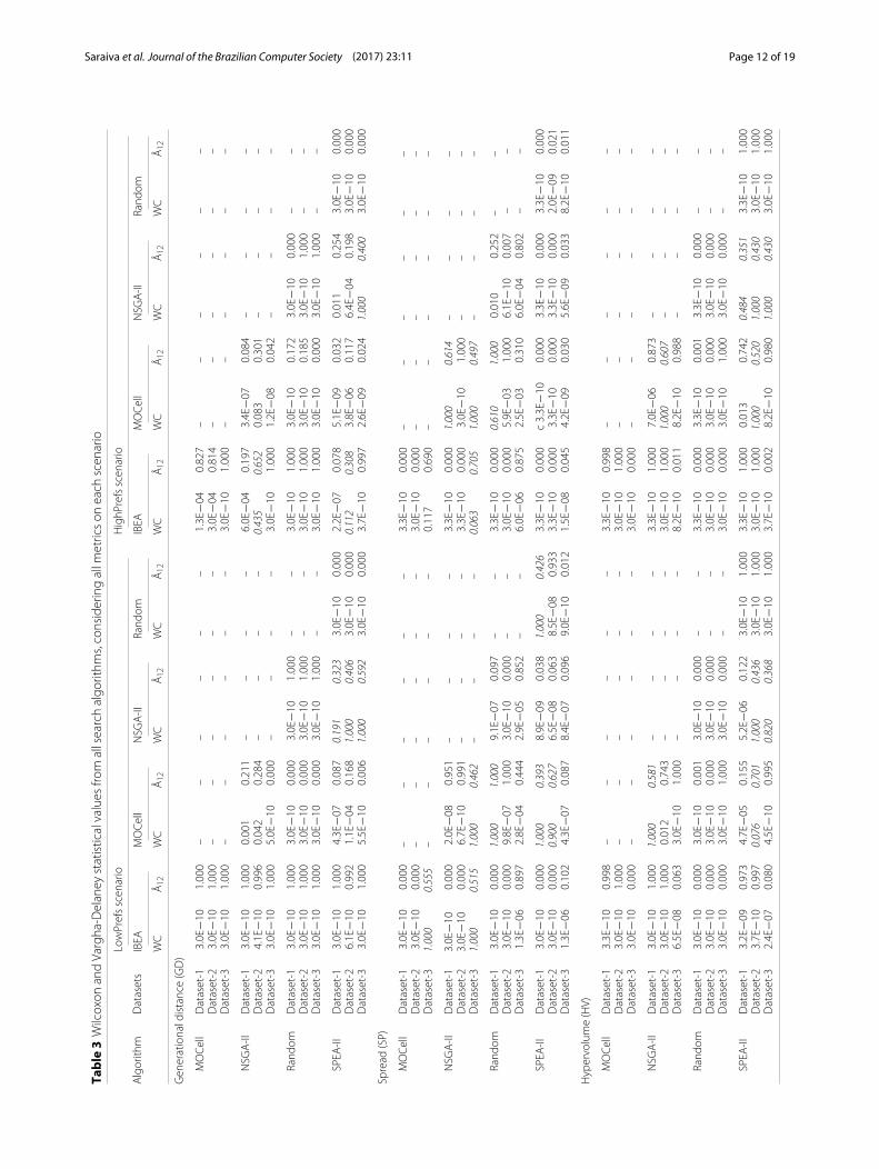
Lastly, in the fourth stage (“Feedbacks”), we obtainedfeedback about how convinced the participants wereabout the subjective satisfaction provided by both solu-tions selected in stages 2 and 3, respectively called non-preference-based and preference-based solutions. As seenin Fig. 7, the participant simply estimates such evalu-ation to each solution on a scale of “Very ineffective,”“Ineffective,” “Indifferent,” “Effective,” and “Very effective.”
Research questionsThree research questions were asked to assess and analyzeour approach behavior. They are presented as follows:
• RQ1: Which search-based techniques, among theevaluated ones, produce better solutions?
• RQ2: Which is the subjective benefit whenconsidering the DM’s preferences as an objective tobe optimized?
• RQ3: Which is the relation between the inclusion ofthe preferences and the DM’s subjective evaluation inthe final solution?
Results and analysisThe results of the empirical study are presented inthis section by analyzing the previous three researchquestions.
• RQ1: Which search-based techniques, among theevaluated ones, produce better solutions?
Fig. 3 GUI used in the “Non-preferences” stage of participant-based experiment
Saraiva et al. Journal of the Brazilian Computer Society (2017) 23:11 Page 10 of 19
Fig. 4 Interface for visualizing solutions from the Pareto front
Aiming to answer this question, we analyzed the resultsproduced by all algorithms for each instance and the sce-nario previously presented in the automatic experimentdesign.Table 3 presents the values of statistical tests con-
sidering the metrics hypervolume (HV), spread (SP),
and generational distance (GD) for each dataset. TheWilcoxon test (WC) was applied, using the Bonferronicorrection, to identify the occurrence of statistical differ-ences among the samples considering a confidence levelof 95%. The Vargha-Delaney Â12 test was used to measurethe effect size, in other words, the relative number of
Fig. 5 GUI used in the “Preferences Set” stage of participant-based experiment
Saraiva et al. Journal of the Brazilian Computer Society (2017) 23:11 Page 11 of 19
Fig. 6 Example of preferences defined by the DM. a Coupling Joint. b Positioning Before. c Positioning Follow
times that an algorithm produced superior values overanother. Further details about each statistical test may beseen in the work of Arcuri and Briand [33]. Â12 mea-sures the probability that a technique (table line) with aparticular parameter setting yields a higher result than
another technique (table column). For instance, consider-ing MOCell (1) and IBEA (2), the probability of MOCellreturning a front better than IBEA’s one according to theGD metric for dataset-1 in HighPrefs is 82.7% given thatthe corresponding Â12 is 0.827.
Fig. 7 GUI presented to the DM in the fourth stage, i.e., “Feedbacks”
Saraiva et al. Journal of the Brazilian Computer Society (2017) 23:11 Page 12 of 19
Table
3Wilcoxon
andVargha-Delaney
statisticalvalues
from
allsearchalgo
rithm
s,consideringallm
etricson
each
scen
ario
Algorith
mDatasets
LowPrefsscen
ario
HighP
refsscen
ario
IBEA
MOCell
NSG
A-II
Rand
omIBEA
MOCell
NSG
A-II
Rand
om
WC
Â12
WC
Â12
WC
Â12
WC
Â12
WC
Â12
WC
Â12
WC
Â12
WC
Â12
Gen
erationaldistance(GD)
MOCell
Dataset-1
3.0E
−10
1.000
––
––
––
1.3E
−04
0.827
––
––
––
Dataset-2
3.0E
−10
1.000
––
––
––
3.0E
−04
0.814
––
––
––
Dataset-3
3.0E
−10
1.000
––
––
––
3.0E
−10
1.000
––
––
––
NSG
A-II
Dataset-1
3.0E
−10
1.000
0.001
0.211
––
––
6.0E
−04
0.197
3.4E
−07
0.084
––
––
Dataset-2
4.1E
−10
0.996
0.042
0.284
––
––
0.435
0.652
0.083
0.301
––
––
Dataset-3
3.0E
−10
1.000
5.0E
−10
0.000
––
––
3.0E
−10
1.000
1.2E
−08
0.042
––
––
Rand
omDataset-1
3.0E
−10
1.000
3.0E
−10
0.000
3.0E
−10
1.000
––
3.0E
−10
1.000
3.0E
−10
0.172
3.0E
−10
0.000
––
Dataset-2
3.0E
−10
1.000
3.0E
−10
0.000
3.0E
−10
1.000
––
3.0E
−10
1.000
3.0E
−10
0.185
3.0E
−10
1.000
––
Dataset-3
3.0E
−10
1.000
3.0E
−10
0.000
3.0E
−10
1.000
––
3.0E
−10
1.000
3.0E
−10
0.000
3.0E
−10
1.000
––
SPEA
-IIDataset-1
3.0E
−10
1.000
4.3E
−07
0.087
0.191
0.323
3.0E
−10
0.000
2.2E
−07
0.078
5.1E
−09
0.032
0.011
0.254
3.0E
−10
0.000
Dataset-2
6.1E
−10
0.992
1.1E
−04
0.168
1.000
0.406
3.0E
−10
0.000
0.112
0.308
3.8E
−06
0.117
6.4E
−04
0.198
3.0E
−10
0.000
Dataset-3
3.0E
−10
1.000
5.5E
−10
0.006
1.000
0.592
3.0E
−10
0.000
3.7E
−10
0.997
2.6E
−09
0.024
1.000
0.400
3.0E
−10
0.000
Spread
(SP)
MOCell
Dataset-1
3.0E
−10
0.000
––
––
––
3.3E
−10
0.000
––
––
––
Dataset-2
3.0E
−10
0.000
––
––
––
3.0E
−10
0.000
––
––
––
Dataset-3
1.000
0.555
––
––
––
0.117
0.690
––
––
––
NSG
A-II
Dataset-1
3.0E
−10
0.000
2.0E
−08
0.951
––
––
3.3E
−10
0.000
1.000
0.614
––
––
Dataset-2
3.0E
−10
0.000
6.7E
−10
0.991
––
––
3.3E
−10
0.000
3.0E
−10
1.000
––
––
Dataset-3
1.000
0.515
1.000
0.462
––
––
0.063
0.705
1.000
0.497
––
––
Rand
omDataset-1
3.0E
−10
0.000
1.000
1.000
9.1E
−07
0.097
––
3.3E
−10
0.000
0.610
1.000
0.010
0.252
––
Dataset-2
3.0E
−10
0.000
9.8E
−07
1.000
3.0E
−10
0.000
––
3.0E
−10
0.000
5.9E
−03
1.000
6.1E
−10
0.007
––
Dataset-3
1.3E
−06
0.897
2.8E
−04
0.444
2.9E
−05
0.852
––
6.0E
−06
0.875
2.5E
−03
0.310
6.0E
−04
0.802
––
SPEA
-IIDataset-1
3.0E
−10
0.000
1.000
0.393
8.9E
−09
0.038
1.000
0.426
3.3E
−10
0.000
c3.3E
−10
0.000
3.3E
−10
0.000
3.3E
−10
0.000
Dataset-2
3.0E
−10
0.000
0.900
0.627
6.5E
−08
0.063
8.5E
−08
0.933
3.3E
−10
0.000
3.3E
−10
0.000
3.3E
−10
0.000
2.0E
−09
0.021
Dataset-3
1.3E
−06
0.102
4.3E
−07
0.087
8.4E
−07
0.096
9.0E
−10
0.012
1.5E
−08
0.045
4.2E
−09
0.030
5.6E
−09
0.033
8.2E
−10
0.011
Hypervolume(HV)
MOCell
Dataset-1
3.3E
−10
0.998
––
––
––
3.3E
−10
0.998
––
––
––
Dataset-2
3.0E
−10
1.000
––
––
––
3.0E
−10
1.000
––
––
––
Dataset-3
3.0E
−10
0.000
––
––
––
3.0E
−10
0.000
––
––
––
NSG
A-II
Dataset-1
3.0E
−10
1.000
1.000
0.581
––
––
3.3E
−10
1.000
7.0E
−06
0.873
––
––
Dataset-2
3.0E
−10
1.000
0.012
0.743
––
––
3.0E
−10
1.000
1.000
0.607
––
––
Dataset-3
6.5E
−08
0.063
3.0E
−10
1.000
––
––
8.2E
−10
0.011
8.2E
−10
0.988
––
––
Rand
omDataset-1
3.0E
−10
0.000
3.0E
−10
0.001
3.0E
−10
0.000
––
3.3E
−10
0.000
3.3E
−10
0.001
3.3E
− 10
0.000
––
Dataset-2
3.0E
−10
0.000
3.0E
−10
0.000
3.0E
−10
0.000
––
3.0E
−10
0.000
3.0E
−10
0.000
3.0E
−10
0.000
––
Dataset-3
3.0E
−10
0.000
3.0E
−10
1.000
3.0E
−10
0.000
––
3.0E
−10
0.000
3.0E
−10
1.000
3.0E
−10
0.000
––
SPEA
-IIDataset-1
3.2E
−09
0.973
4.7E
−05
0.155
5.2E
−06
0.122
3.0E
−10
1.000
3.3E
−10
1.000
0.013
0.742
0.484
0.351
3.3E
−10
1.000
Dataset-2
3.7E
−10
0.997
0.076
0.701
1.000
0.436
3.0E
−10
1.000
3.0E
−10
1.000
1.000
0.520
1.000
0.430
3.0E
−10
1.000
Dataset-3
2.4E
−07
0.080
4.5E
−10
0.995
0.820
0.368
3.0E
−10
1.000
3.7E
−10
0.002
8.2E
−10
0.980
1.000
0.430
3.0E
−10
1.000
Saraiva et al. Journal of the Brazilian Computer Society (2017) 23:11 Page 13 of 19
Observing the data from Table 3, it is noticeable thatthere was a statistical difference in most of the compar-isons, except for 14.4% of the times in which there was nostatistical difference (values in italic).Before analyzing the results obtained from the GD met-
ric, it is important to highlight that a value close to 0 isdesirable because it indicates that the Pareto front is closerto the PFref. Thus, looking at dataset-1 and LowPref sce-nario, we can note that IBEA achieved better results ofGD, due to Â12 being 1 when the other algorithms arecompared with IBEA. This means that 100% of the times,other techniques produced results higher than IBEA, forthe GD metric. Such a behavior is verified in almost allof the scenarios. However, in dataset-1, when the numberof preferences is high, IBEA lost to NSGA-II. Therefore,in general, IBEA outperforms all the other algorithmsin terms of GD, and NSGA-II is the second best searchtechnique among the evaluated ones.As noted in the “Automatic experiment” section, the
metric SP measures the dispersion between the Paretofront solutions. In practice, lower values for this metricbring about more uniformly distributed solutions fromthe front. Thus, observing the statistical test results forSP, we can see that IBEA achieves the worst results 100%of the times in comparison with all the other techniquesfor each scenario of dataset-1 and dataset-2. This obser-vation indicates that even solutions returned by IBEA arenext to the reference Pareto front. However, these solu-tions are not well distributed in the search space. On theother hand, SPEA-II obtained the best results in SP forall instances, although no statistical difference was veri-fied in dataset-1 and dataset-2 with low preferences whencompared with MOCell.Observing both approximations to the PFref (conver-
gence) and diversity, hypervolume (HV) is essential forevaluating the multi-objective algorithms. Because the
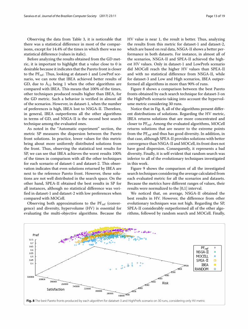
HV value is near 1, the result is better. Thus, analyzingthe results from this metric for dataset-1 and dataset-2,which are based on real data, NSGA-II shows a better per-formance in both datasets. For instance, in almost all ofthe scenarios, NSGA-II and SPEA-II achieved the high-est HV values. Only in dataset-1 and LowPrefs scenariodid MOCell reach the higher HV values than SPEA-IIand with no statistical difference from NSGA-II, whilefor dataset-3 and Low and High scenarios, IBEA outper-formed all algorithms in more than 90% of runs.Figure 8 shows a comparison between the best Pareto
fronts obtained by each search technique for dataset-3 onthe HighPrefs scenario taking into account the hypervol-ume metric considering 30 runs.Notice that in Fig. 8, all of the algorithms present differ-
ent distributions of solutions. Regarding the HV metric,IBEA returns solutions that are more concentrated andcloser to PFref. Among the evaluated algorithms, MOCellreturns solutions that are nearer to the extreme pointsfrom the PFref and thus has good diversity. In addition, inthat case, although SPEA-II provides solutions with betterconvergence thanNSGA-II andMOCell, its front does nothave good dispersion. Consequently, it represents a baddiversity. Finally, it is self-evident that random search wasinferior to all of the evolutionary techniques investigatedin this work.Figure 9 shows the comparison of all the investigated
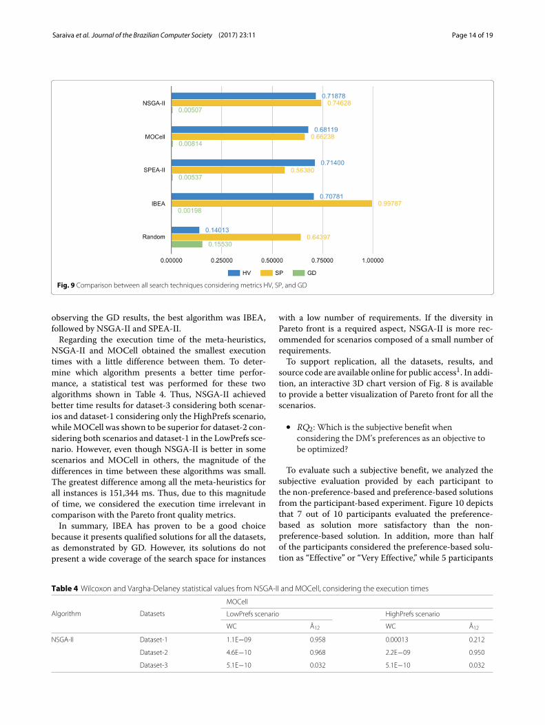
search techniques considering the average calculated fromeach evaluated metric for all the scenarios and datasets.Because the metrics have different ranges of values, theirresults were normalized to the [0,1] interval.We noticed that, on average, NSGA-II obtained the
best results in HV. However, the difference from otherevolutionary techniques was not high. Regarding the SP,SPEA-II considerably outperformed all of the other algo-rithms, followed by random search and MOCell. Finally,
Fig. 8 The best Pareto fronts produced by each algorithm for datatset-3 and HighPrefs scenario on 30 runs, considering only HV metric
Saraiva et al. Journal of the Brazilian Computer Society (2017) 23:11 Page 14 of 19
Fig. 9 Comparison between all search techniques considering metrics HV, SP, and GD
observing the GD results, the best algorithm was IBEA,followed by NSGA-II and SPEA-II.Regarding the execution time of the meta-heuristics,
NSGA-II and MOCell obtained the smallest executiontimes with a little difference between them. To deter-mine which algorithm presents a better time perfor-mance, a statistical test was performed for these twoalgorithms shown in Table 4. Thus, NSGA-II achievedbetter time results for dataset-3 considering both scenar-ios and dataset-1 considering only the HighPrefs scenario,whileMOCell was shown to be superior for dataset-2 con-sidering both scenarios and dataset-1 in the LowPrefs sce-nario. However, even though NSGA-II is better in somescenarios and MOCell in others, the magnitude of thedifferences in time between these algorithms was small.The greatest difference among all the meta-heuristics forall instances is 151,344 ms. Thus, due to this magnitudeof time, we considered the execution time irrelevant incomparison with the Pareto front quality metrics.In summary, IBEA has proven to be a good choice
because it presents qualified solutions for all the datasets,as demonstrated by GD. However, its solutions do notpresent a wide coverage of the search space for instances
with a low number of requirements. If the diversity inPareto front is a required aspect, NSGA-II is more rec-ommended for scenarios composed of a small number ofrequirements.To support replication, all the datasets, results, and
source code are available online for public access1. In addi-tion, an interactive 3D chart version of Fig. 8 is availableto provide a better visualization of Pareto front for all thescenarios.
• RQ2: Which is the subjective benefit whenconsidering the DM’s preferences as an objective tobe optimized?
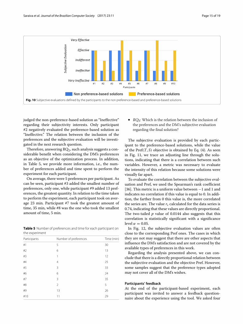
To evaluate such a subjective benefit, we analyzed thesubjective evaluation provided by each participant tothe non-preference-based and preference-based solutionsfrom the participant-based experiment. Figure 10 depictsthat 7 out of 10 participants evaluated the preference-based as solution more satisfactory than the non-preference-based solution. In addition, more than halfof the participants considered the preference-based solu-tion as “Effective” or “Very Effective,” while 5 participants
Table 4 Wilcoxon and Vargha-Delaney statistical values from NSGA-II and MOCell, considering the execution times
Algorithm Datasets
MOCell
LowPrefs scenario HighPrefs scenario
WC Â12 WC Â12
NSGA-II Dataset-1 1.1E−09 0.958 0.00013 0.212
Dataset-2 4.6E−10 0.968 2.2E−09 0.950
Dataset-3 5.1E−10 0.032 5.1E−10 0.032
Saraiva et al. Journal of the Brazilian Computer Society (2017) 23:11 Page 15 of 19
Fig. 10 Subjective evaluations defined by the participants to the non preference-based and preference-based solutions
judged the non-preference-based solution as “Ineffective”regarding their subjectivity interests. Only participant#2 negatively evaluated the preference-based solution as“Ineffective.” The relation between the inclusion of thepreferences and the subjective evaluation will be investi-gated in the next research question.Therefore, answering RQ2, such analysis suggests a con-
siderable benefit when considering the DM’s preferencesas an objective of the optimization process. In addition,in Table 5, we provide more information, i.e., the num-ber of preferences added and time spent to perform theexperiment for each participant.On average, there were 5 preferences per participant. As
can be seen, participant #3 added the smallest number ofpreferences, only one, while participant #9 added 13 pref-erences, the greatest quantity. In relation to the time takento perform the experiment, each participant took on aver-age 23 min. Participant #7 took the greatest amount oftime, 35 min, while #8 was the one who took the smallestamount of time, 5 min.
Table 5 Number of preferences and time for each participant onthe experiment
Participants Number of preferences Time (min)
#1 5 30
#2 6 13
#3 1 12
#4 4 25
#5 3 33
#6 6 24
#7 3 35
#8 2 5
#9 13 26
#10 11 29
• RQ3: Which is the relation between the inclusion ofthe preferences and the DM’s subjective evaluationregarding the final solution?
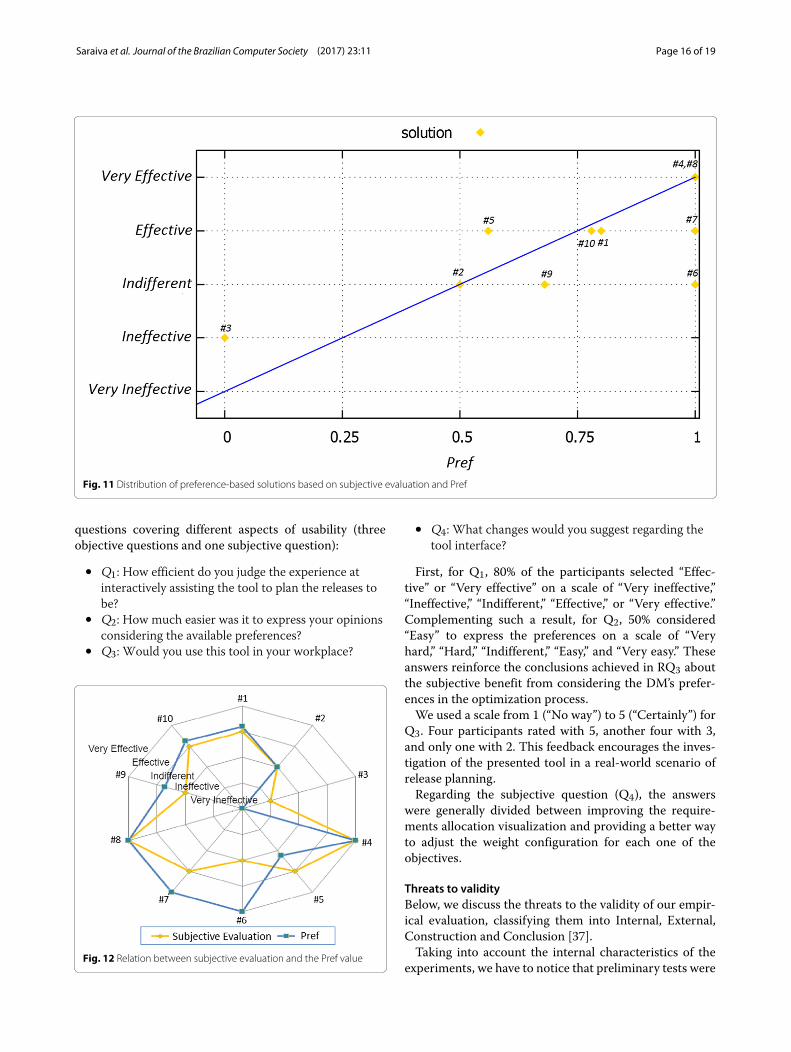
The subjective evaluation is provided by each partic-ipant to the preference-based solutions, while the valueof the Pref(T , S) objective is obtained by Eq. (4). As seenin Fig. 11, we trace an adjusting line through the solu-tions, indicating that there is a correlation between suchvariables. However, a metric was necessary to evaluatethe intensity of this relation because some solutions werevisually far apart.To evaluate the correlation between the subjective eval-
uation and Pref, we used the Spearman’s rank coefficient[36]. This metric is a uniform value between −1 and 1 andindicates no correlation if this value is equal to 0. In addi-tion, the farther from 0 this value is, the more correlatedthe series are. The value rs calculated for the data series is0.74, indicating that these values are directly proportional.The two-tailed p value of 0.0144 also suggests that thiscorrelation is statistically significant with a significancelevel α = 0.05.In Fig. 12, the subjective evaluation values are often
close to the corresponding Pref ones. The cases in whichthey are not may suggest that there are other aspects thatinfluence the DM’s satisfaction and are not covered by theavailable types of preferences in this work.Regarding the analysis presented above, we can con-
clude that there is a directly proportional relation betweenthe subjective evaluation and the objective Pref. However,some samples suggest that the preference types adoptedmay not cover all of the DM’s wishes.
Participants’ feedbackAt the end of the participant-based experiment, eachparticipant was invited to answer a feedback question-naire about the experience using the tool. We asked four
Saraiva et al. Journal of the Brazilian Computer Society (2017) 23:11 Page 16 of 19
Fig. 11 Distribution of preference-based solutions based on subjective evaluation and Pref
questions covering different aspects of usability (threeobjective questions and one subjective question):
• Q1: How efficient do you judge the experience atinteractively assisting the tool to plan the releases tobe?
• Q2: How much easier was it to express your opinionsconsidering the available preferences?
• Q3: Would you use this tool in your workplace?
Fig. 12 Relation between subjective evaluation and the Pref value
• Q4: What changes would you suggest regarding thetool interface?
First, for Q1, 80% of the participants selected “Effec-tive” or “Very effective” on a scale of “Very ineffective,”“Ineffective,” “Indifferent,” “Effective,” or “Very effective.”Complementing such a result, for Q2, 50% considered“Easy” to express the preferences on a scale of “Veryhard,” “Hard,” “Indifferent,” “Easy,” and “Very easy.” Theseanswers reinforce the conclusions achieved in RQ3 aboutthe subjective benefit from considering the DM’s prefer-ences in the optimization process.We used a scale from 1 (“No way”) to 5 (“Certainly”) for
Q3. Four participants rated with 5, another four with 3,and only one with 2. This feedback encourages the inves-tigation of the presented tool in a real-world scenario ofrelease planning.Regarding the subjective question (Q4), the answers
were generally divided between improving the require-ments allocation visualization and providing a better wayto adjust the weight configuration for each one of theobjectives.
Threats to validityBelow, we discuss the threats to the validity of our empir-ical evaluation, classifying them into Internal, External,Construction and Conclusion [37].Taking into account the internal characteristics of the
experiments, we have to notice that preliminary tests were
Saraiva et al. Journal of the Brazilian Computer Society (2017) 23:11 Page 17 of 19
carried out for defining the search technique parametriza-tion. However, some specific settings on a given algorithmcan obtain better results for some instances. Despite thefact that two datasets were based on real data, some infor-mation was necessary to be randomly generated (risk val-ues and number of releases), that is, they do not representa fully real-world scenario. The risk of implementing eachrequirement, which did not originally exist, was manuallydefined by a Developer and appended to the instances.The number of releases was changed from 3 to 5 and 8for dataset-1 and dataset-2, respectively. This choice wasmade to increase the variation of the DM’s preferences.Regarding the participant-based experiment, the par-
ticipants may have changed their behavior since theyknew that they were under evaluation, corroborating theHawthorne’s effect [38]. To mitigate this problem, the par-ticipants received an explanation about the approach butnot about the assumptions that were under investigation.We believe that our empirical study has a weakness
regarding the generalization of the achieved results. Forinstance, the datasets based on real information have fewrequirements, which makes it hard to conclude that theresults would be similar for large-scale instances. Such acircumstance was the motivation to generate and use theartificial dataset with a large number of requirements. Asimilar problem is encountered in the participant-basedexperiment because the number of participants was nothigh enough to represent expressive scenarios.Concerning the experiment construction threats, the
metrics that we used to estimate client’s satisfaction andoverall risk are based on values that are defined a pri-ori by the development team. These estimated values mayvary as the project goes on, which requires rerunningthe approach to adapt these changes. Despite this limita-tion, this strategy is widely used in the literature, such as[3, 39, 40]. In addition, it is known that meta-heuristicscan vary their final solutions and execution time accord-ing to the instance. Unfortunately, we did not investigatetime concerns. In addition, there is no longer an expla-nation about the evaluated metrics. Nevertheless, all ofthem have been widely used in the related works as well asthe multi-objective optimization literature. Still, consid-ering the participant-based experiment, the major metricused to measure the satisfaction of each participant wasa subjective evaluation provided for the final solutionfollowing a scale of “Very ineffective,” “Ineffective,” “Indif-ferent,” “Effective,” and “Very effective.” This feedback maynot properly represent the DM’s feeling.Finally, the threats to the experiment conclusions’ valid-
ity are mainly related to the characteristics of the algo-rithms that were investigated. Meta-heuristics present astochastic behavior, and thus, distinct runs may producedifferent results for the same problem. Aiming at mini-mizing such a weakness, for each combination between
datasets, scenarios and the DM’s preferences for thesearch algorithmswere executed 30 times in the automaticexperiment. Given all obtained results, we conducted sta-tistical analyses as recommended by Arcuri and Briand[41]. Analyzing the conclusions of the participant-basedexperiment, some of themmay be affected by each partic-ipant’s understanding level after receiving an explanationabout the study as well as their experience on releaseplanning using automatic tools.
ConclusionsRelease planning is one of the most complex and relevantactivities performed in the iterative and incremental soft-ware development process. Recently, the SBSE approacheshave been discussed based on the strength of the com-putational intelligence with the human expertise. In otherwords, it allows the search process to be guided by thehuman’s knowledge and, consequently, provide valuablesolutions to the decision maker (DM). Thus, we claimthe importance of providing a mechanism to capture theDM preferences in a broader scope, instead of just requir-ing a weight factor, for instance. Besides increasing thehuman’s engagement, he/she will progressively gain moreconsciousness of how feasible the preferences are.The evaluated multi-objective approach consists of
treating the human’s preferences as another objective tobe maximized, as well as maximizing the overall client sat-isfaction and minimizing the project risk. In sum, the DMdefines a set of preferences about the requirements alloca-tion, which are stored in a preference base responsible forinfluencing the search process.Therefore, we have significantly extended our previous
work through the accomplishment of new experimen-tal analysis considering both simulated and real humanevaluations. The automatic experiment points out thatNSGA-II obtained overall superiority in two of the threedatasets investigated, positioning itself as a good searchtechnique for smaller scenarios, while IBEA showed a bet-ter performance for large datasets, since the loss in the ini-tial diversity of the algorithm decreases as the number ofrequirements increases. Regarding the participant-basedexperiment, it was found that two thirds of the partici-pants evaluated the preference-based solution better thanthe non-preference-based one, encouraging the investi-gation of the presented tool in a real-world scenario ofrelease planning. In addition, we made a novel tool forthe release planning process to be able to incorporate thehuman preferences during the optimization process1.As future work, we intend to evolve our GUI to provide
a more intuitive interaction, solutions visualization andpreferences specification by the DM. We also intend tocompare our approach with other search-based proposals,which explore the human’s preferences in the optimizationprocess.
Saraiva et al. Journal of the Brazilian Computer Society (2017) 23:11 Page 18 of 19
Endnote1Webpage: http://goes.uece.br/raphaelsaraiva/multi4rp/en/.
AbbreviationsDM: Decision maker; EA: Evolutionary algorithm; GD: Generational distance;HV: Hypervolume; IBEA: Indicator-based evolutionary algorithm; MOCell:Multi-objective cellular genetic algorithm; NRP: Next release problem; NSGA-II:Nondominated sorting genetic algorithm II; PFtrue: Pareto front; PFref:Reference Pareto front; RP: Release planning; SBSE: Search-based softwareengineering; SP: Spread; SPEA-II: Strength Pareto evolutionary algorithm II
AcknowledgementsThe authors acknowledged all the participants for their availability to theexperiment.
FundingWe would like to thank the Foundation of Scientific and TechnologicalDevelopment Supporting from Ceará (FUNCAP) for the financial support.
Availability of data andmaterialsThe datasets and results supporting the conclusions of this article are availableat webpage: http://goes.uece.br/raphaelsaraiva/multi4rp/en/.
Authors’ contributionsAll authors have contributed to the methodological and experimental aspectsof the research. The authors have also read and approved the final manuscript.
Competing interestsThe authors declare that they have no competing interests.
Publisher’s NoteSpringer Nature remains neutral with regard to jurisdictional claims inpublished maps and institutional affiliations.
Author details1State University of Ceará, Dr. Silas Munguba Avenue, 1700 Fortaleza, CE, Brazil.2Federal University of Ceará, Cratéus, CE, Brazil. 3Federal University of Goiás,Goiânia, GO, Brazil.
Received: 9 January 2017 Accepted: 10 July 2017
References1. Sommerville I (2011) Software engineering. Addison Wesley, Boston2. Ngo-The A, Ruhe G (2008) A systematic approach for solving the wicked
problem of software release planning. Soft Comput Fusion FoundMethodologies Appl 12(1):95–108
3. Ruhe G, Saliu MO (2005) The art and science of software release planning.Softw IEEE 22(6):47–53
4. Harman M, McMinn P, de Souza JT, Yoo S (2012) Search based softwareengineering: techniques, taxonomy, tutorial. Empir Softw Eng Verification7007:1–59
5. Miettinen K (2012) Nonlinear multiobjective optimization, Vol. 12.Springer, New York
6. Zhang Y, Finkelstein A, Harman M (2008) Search based requirementsoptimisation: existing work & challenges. In: Proceedings of the 14thInternational Working Conference, Requirements Engineering:Foundation for Software Quality (RefsQ ’08). Springer, MontpellierVol. 5025. pp 88–94
7. Marculescu B, Poulding S, Feldt R, Petersen K, Torkar R (2016) Testerinteractivity makes a difference in search-based software testing: Acontrolled experiment. Inf Softw Technol 78:66–82
8. Araújo AA, Paixao M, Yeltsin I, Dantas A, Souza J (2016) An Architecturebased on interactive optimization and machine learning applied to thenext release problem. Autom Softw Eng 3(24):623–671
9. Ferreira TdN, Arajo AA, Baslio Neto AD, de Souza JT (2016) Incorporatinguser preferences in ant colony optimization for the next release problem.Appl Soft Comput 49(C):1283–1296
10. Tonella P, Susi A, Palma F (2013) Interactive requirements prioritizationusing a genetic algorithm. Inf Softw Technol 55(1):173–187
11. Dantas A, Yeltsin I, Araújo AA, Souza J (2015) Interactive software releaseplanning with preferences base. In: International Symposium on SearchBased Software Engineering. Springer, Cham. pp 341–346
12. Saraiva R, Araújo AA, Dantas A, Souza J (2016) Uma AbordagemMultiobjetivo baseada em Otimização Interativa para o Planejamento deReleases. In: VII Workshop em Engenharia de Software Baseada em Busca.CBSoft, Maringá
13. Wierzbicki AP (1980) The use of reference objectives in multiobjectiveoptimization. In: Multiple Criteria Decision Making Theory andApplication. Springer, West Germany Vol. 117. pp 468–486
14. Harman M, Jones BF (2001) Search-based software engineering. Inf SoftwTechnol 43(14):833–839
15. Harman Mark (2007) The current state and future of search basedsoftware engineering. In: 2007 Future of Software Engineering. IEEEComputer Society, Washington. pp 342–357
16. Pitangueira AM, Maciel RSP, de Oliveira Barros M (2015) Softwarerequirements selection and prioritization using sbse approaches: asystematic review andmapping of the literature. J Syst Softw 103:267–280
17. Räihä O (2010) A survey on search-based software design. Comput SciRev 4(4):203–249
18. McMinn P (2004) Search-based software test data generation: a survey.Softw Testing Verification Reliab 14(2):105–156
19. Harman M, Mansouri SA, Zhang Y (2009) Search based softwareengineering: a comprehensive analysis and review of trends techniquesand applications. Department of Computer Science, King’s CollegeLondon, Tech. Rep. TR-09-03
20. Back T (1996) Evolutionary algorithms in theory and practice: evolutionstrategies, evolutionary programming, genetic algorithms. Oxforduniversity press, New York
21. Deb K, Pratap A, Agarwal S, Meyarivan T (2002) A fast and elitistmultiobjective genetic algorithm: Nsga-ii. IEEE Trans Evol Comput6(2):182–197
22. Nebro AJ, Durillo JJ, Luna F, Dorronsoro B, Alba E (2009) Mocell: a cellulargenetic algorithm for multiobjective optimization. Int J Intell Syst24(7):726–746
23. Zitzler E, Künzli S (2004) Indicator-based selection in multiobjectivesearch. In: International Conference on Parallel Problem Solving fromNature. Springer, Berlin. pp 832–842
24. Zitzler E, Laumanns M, Thiele L, et al (2001) SPEA2: Improving the strengthPareto evolutionary algorithm. In: Eurogen. ETH-TIK, Zürich Vol. 3242(103).pp 95–100
25. Baker P, Harman M, Steinhofel K, Skaliotis A (2006) Search basedapproaches to component selection and prioritization for the nextrelease problem. In: 2006 22nd IEEE International Conference on SoftwareMaintenance. IEEE, Philadelphia. pp 176–185
26. Boehm BW (1991) Software risk management: principles and practices.IEEE Softw 8(1):32–41
27. Brasil MMA, da Silva TGN, de Freitas FG, de Souza JT, Cortés MI (2012) AMultiobjective Optimization Approach to the Software Release Planningwith Undefined Number of Releases and Interdependent Requirements.In: Enterprise Information Systems: 13th International Conference, ICEIS2011, Revised Selected Papers. Springer, Beijing Vol. 102. p 300
28. Deb K (2001) Multi-objective optimization using evolutionary algorithms,Vol. 16. John Wiley & Sons, United Kingdom
29. Thiele L, Miettinen K, Korhonen PJ, Molina J (2009) A preference-basedevolutionary algorithm for multi-objective optimization. Evol Comput17(3):411–436
30. Kitchenham BA, Pfleeger SL, Pickard LM, Jones PW, Hoaglin DC, Emam KE,Rosenberg J (2002) Preliminary guidelines for empirical research insoftware engineering. IEEE Trans Softw Eng 28(8):721–734
31. Yin RK (2003) Case study research: Design and methods. In: Applied SocialResearch Methods Series. Sage Publications, California Vol. 5
32. Karim MR, Ruhe G (2014) Bi-objective genetic search for release planningin support of themes. In: SSBSE’14. Springer, Cham. pp 123–137
33. Arcuri A, Briand L (2014) A hitchhiker’s guide to statistical tests forassessing randomized algorithms in software engineering. Softw TestingVerification Reliab 24(3):219–250
34. Zhang Y (2010) Multi-objective search-based requirements selection andoptimisation. University of London, London
Saraiva et al. Journal of the Brazilian Computer Society (2017) 23:11 Page 19 of 19
35. ZITZLER E (1999) Evolutionary Algorithms for Multiobjective Optimization:Methods and Applications. Swiss Fed Inst Technol (ETH) Zurich.TIK-Schriftenr 30
36. Siegel S (1956) Nonparametric statistics for the behavioral sciences. 1stedn. McGraw-Hill, Columbus
37. de Oliveira Barros M, Dias-Neto AC (2011) 0006/2011-Threats to Validity inSearch-based Software Engineering Empirical Studies. RelaTe-DIA5(1):1–12
38. McCambridge J, Witton J, Elbourne DR (2014) Systematic review of thehawthorne effect: new concepts are needed to study researchparticipation effects. J Clin Epidemiol 67(3):267–277
39. Colares F, Souza J, Carmo R, Pádua C, Mateus GR (2009) A new approachto the software release planning. In: Software Engineering, 2009. SBES’09.XXIII Brazilian Symposium on. IEEE, New York. pp 207–215
40. Greer D, Ruhe G (2004) Software release planning: an evolutionary anditerative approach. Inf Softw Technol 46(4):243–253
41. Arcuri A, Briand L (2011) A practical guide for using statistical tests toassess randomized algorithms in software engineering. In: 2011 33rdInternational Conference on Software Engineering (ICSE). IEEE, New York.pp 1–10