RESEARCH Open Access Particle filter track-before-detect

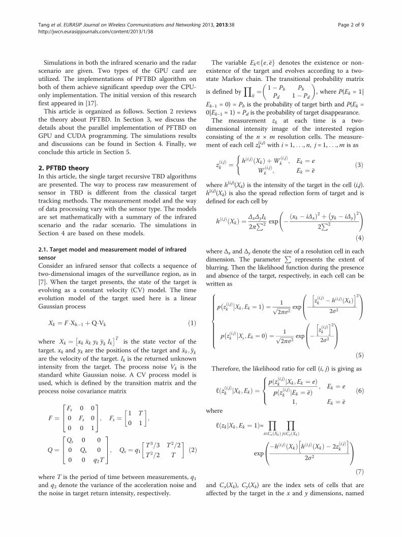
Tang et al. EURASIP Journal on Wireless Communications and Networking 2013, 2013:38http://jwcn.eurasipjournals.com/content/2013/1/38

RESEARCH Open Access

Particle filter track-before-detect implementationon GPUXu Tang*, Jinzhou Su, Fangbin Zhao, Jian Zhou and Ping Wei

Abstract

Track-before-detect (TBD) based on the particle filter (PF) algorithm is known for its outstanding performance indetecting and tracking of weak targets. However, large amount of calculation leads to difficulty in real-timeapplications. To solve this problem, effective implementation of the PF-based TBD on the graphics processing units(GPU) is proposed in this article. By recasting the particles propagation process and weights calculating process onthe parallel structure of GPU, the running time of this algorithm can greatly be reduced. Simulation results in theinfrared scenario and the radar scenario are demonstrated to compare the implementation on two types of theGPU card with the CPU-only implementation.

Keywords: Track-before-detect, Particle filter, GPU

1. IntroductionClassical target detection and tracking is performed onthe basis of pre-processed measurements, which arecomposed of the threshold output of the sensor. Inthis way, no effective integrations over time can betaken place and much information is lost. To avoidthis problem, the track-before-detect (TBD) techniqueis developed to use directly the un-threshold or lowthreshold measurements of sensors to utilize the rawinformation. The TBD-based procedures jointly processmore consecutive measurements, thus can increase thesignal-to-noise ratio (SNR), and realize the detectionand tracking of weak targets simultaneously.The scenarios faced by TBD are almost nonlinear and

non-Gaussian, so the particle filter (PF) [1] is a reason-able solution. The PF is a Monte Carlo simulationmethod and widely used in target tracking of linear ornonlinear dynamic systems [2,3]. Salmond and coauthors[4,5] first introduced the PF implementation of TBD(PFTBD) in infrared scenario. Then, Rutten et al. [6-8]proposed several improved PFTBD algorithms. Boersand Driessen [9] extended the work of PFTBD into theradar targets detection and the tracking application.PFTBD algorithms have demonstrated the improvedtrack accuracy and the ability to follow the low SNR

* Correspondence: [email protected] of Electronic Engineering, University of Electronic Science andTechnology of China, Chengdu, People’s Republic of China

© 2013 Tang et al.; licensee Springer. This is anAttribution License (http://creativecommons.orin any medium, provided the original work is p

targets but at the price of an extreme increase of thecomputational complexity.In recent years, the field programmable gate array

(FPGA) and the graphics processing unit (GPU) are themost important architectures in parallel computing. Asthe rapid development of GPU technology, GPU is fam-ous for its significant ability in parallel computing forboth the graphic processing and the general-purposecomputing. Moreover, the compute unified device archi-tecture (CUDA) [10] is introduced to facilitate a hybridutilization of GPU and central process unit (CPU) [11].FPGA has been used to implement PFs, such as in[12,13]. However, with the increasing of number ofparticles, GPU is expected to obtain a better perform-ance than FPGA. More specifically, the PF algorithmshave been implemented on GPU [14-16], and achievesignificant speedup ratio over the implementations onthe traditional CPU fashion but with no losing the per-formance for its float point computation ability.From the best of the authors’ knowledge, no PFTBD

algorithm implemented on GPU is given in the litera-ture. In this article, we propose a novel implementationof PFTBD algorithm on GPU by the CUDA program-ming. Concerned with the difficulty of PFTBD beyondthe PF, new scheme to dispatch the GPU resources forparticles are developed and the programming about thelikelihood ratio area are considered carefully.

Open Access article distributed under the terms of the Creative Commonsg/licenses/by/2.0), which permits unrestricted use, distribution, and reproductionroperly cited.

mailto:[email protected]

http://creativecommons.org/licenses/by/2.0

Tang et al. EURASIP Journal on Wireless Communications and Networking 2013, 2013:38 Page 2 of 9http://jwcn.eurasipjournals.com/content/2013/1/38

Simulations in both the infrared scenario and the radarscenario are given. Two types of the GPU card areutilized. The implementations of PFTBD algorithm onboth of them achieve significant speedup over the CPU-only implementation. The initial version of this researchfirst appeared in [17].This article is organized as follows. Section 2 reviews

the theory about PFTBD. In Section 3, we discuss thedetails about the parallel implementation of PFTBD onGPU and CUDA programming. The simulations resultsand discussions can be found in Section 4. Finally, weconclude this article in Section 5.

2. PFTBD theoryIn this article, the single target recursive TBD algorithmsare presented. The way to process raw measurement ofsensor in TBD is different from the classical targettracking methods. The measurement model and the wayof data processing vary with the sensor type. The modelsare set mathematically with a summary of the infraredscenario and the radar scenario. The simulations inSection 4 are based on these models.

2.1. Target model and measurement model of infraredsensorConsider an infrared sensor that collects a sequence oftwo-dimensional images of the surveillance region, as in[7]. When the target presents, the state of the target isevolving as a constant velocity (CV) model. The timeevolution model of the target used here is a linearGaussian process

Xk ¼ F⋅Xk�1 þQ⋅Vk ð1Þ

where Xk ¼ xk �xk yk �yk Ik� �T

is the state vector of thetarget. xk and yk are the positions of the target and �xk ;�ykare the velocity of the target. Ik is the returned unknownintensity from the target. The process noise Vk is thestandard white Gaussian noise. A CV process model isused, which is defined by the transition matrix and theprocess noise covariance matrix

F ¼Fs 0 0

0 Fs 0

0 0 1

264375; Fs ¼

1 T

0 1

� �;

Q ¼Qs 0 0

0 Qs 0

0 0 q2T

264375; Qs ¼ q1

T 3=3 T 2=2

T 2=2 T

� �ð2Þ

where T is the period of time between measurements, q1and q2 denote the variance of the acceleration noise andthe noise in target return intensity, respectively.

The variable Ek∈ e;�ef g denotes the existence or non-existence of the target and evolves according to a two-state Markov chain. The transitional probability matrix

is defined byY

ij¼ 1� Pb Pb

Pd 1� Pd

� �, where P(Ek = 1|

Ek−1 = 0) = Pb is the probability of target birth and P(Ek =0|Ek−1 = 1) = Pd is the probability of target disappearance.The measurement zk at each time is a two-

dimensional intensity image of the interested regionconsisting of the n × m resolution cells. The measure-ment of each cell zk

(i,j) with i = 1, . . ., n, j = 1, . . .,m is as

z i;jð Þk ¼ h i;jð Þ Xkð Þ þW i;jð Þ

k ; Ek ¼ e

W i;jð Þk ; Ek ¼ �e

(ð3Þ

where h(i,j)(Xk) is the intensity of the target in the cell (i,j).h(i,j)(Xk) is also the spread reflection form of target and isdefined for each cell by

h i;jð Þ Xkð Þ ¼ ΔxΔyIk2πP2 exp � xk � iΔxð Þ2 þ yk � iΔy

� 22P2

!ð4Þ

where Δx and Δy denote the size of a resolution cell in eachdimension. The parameter

Prepresents the extent of

blurring. Then the likelihood function during the presenceand absence of the target, respectively, in each cell can bewritten as

p�z i;jð Þk

Xk ; Ek ¼ 1 ¼ 1ffiffiffiffiffiffiffiffiffiffi

2πσ2p exp �

z i;jð Þk � h i;jð Þ Xkð Þ

h i2σ2

20B@1CA

p�z i;jð Þk

Xk ;Ek ¼ 0 ¼ 1ffiffiffiffiffiffiffiffiffiffi

2πσ2p exp �

z i;jð Þk

h i22σ2

0B@1CA

8>>>>>>>>><>>>>>>>>>:ð5Þ

Therefore, the likelihood ratio for cell (i, j) is giving as

ℓðz i;jð Þk Xk ; Ekj Þ ¼

pðz i;jð Þk Xk ; Ek ¼ ej Þ

pðz i;jð Þk Ek ¼ �ej Þ

; Ek ¼ e

1; Ek ¼ �e

ð6Þ

8><>:where

ℓðzk Xk ;Ek ¼ 1j Þ≈Y

i∈Cx Xkð Þ

Yj∈Cy Xkð Þ

exp�h i;jð Þ Xkð Þ h i;jð Þ Xkð Þ � 2z i;jð Þ

k

h i2σ2

0@ 1Að7Þ

and Cx(Xk), Cy(Xk) are the index sets of cells that areaffected by the target in the x and y dimensions, named


as the likelihood ratio area. The size of them isdetermined by the application parameter, such as theresolution of the observation area and the intensity ofthe target. The bigger likelihood ratio area, the more la-tent target information can be utilized.The measurement noise Wk

(i,j) in each cell is assumedas the independent white Gaussian distribution withzero mean and variance σ2. The SNR for the target isdefined by

SNR ¼ 10 log IkΔxΔy=2πΣ2

� =σ

� �2dBð Þ ð8Þ

2.2. Target model and measurement model of radarsensorDifferent from infrared sensor, the raw measurement dataof radar sensor are always based on range-Doppler-bearingof the signal, as in [9]. The time evolution model of the tar-get used here is also a linear Gaussian process:

Xk ¼ F⋅Xk�1 þQ⋅Vk ð9Þ

where Xk ¼ xk �xk yk �yk� �T

is the state vector of the target.xk and yk are the positions of the target and �xk ;�yk are thevelocity of the target. If we make T as the update time, thenthe transition matrix and the process noise covariancematrix can be defined as

F ¼1 0 T 00 1 0 T0 0 1 00 0 0 1

26643775;

Q ¼1=2 amaxx=3ð ÞT2 0

0 1=2 amaxy=3�

T 2

1=2 amaxx=3ð ÞT 00 1=2 amaxy=3

� T

26643775

ð10Þ

where amaxx, amaxy is the maximum accelerations and theprocess noise Vk is the standard white Gaussian noise.At each discrete time k, the measurement zk is the

reflected power of target. zk is based on the presence ofthe target and is defined by

zk ¼ h Xkð Þ þWk ; Ek ¼ eWk ; Ek ¼ �e

�ð11Þ

In this article, the measurements are modeled aspower levels in range-Doppler-bearing Nr × Nd × Nb

sensor cells. Thus, zk can be defined by zk ¼ fzði;j;lÞk : i =1, . . .,Nr, j = 1, . . .,Nd, l = 1, . . .,Nb}. The power mea-surements per range-Doppler-bearing cell can be definedas zk

(i,j,l) = |zA,k(i,j,l)|2, where zA,k

(i,j,l) represents the complexamplitude data of the target, which is

z i;j;lð ÞA;k ¼ Akh

i;j;lð ÞA Xkð Þ þ nk ; Ek ¼ e

nk ; Ek ¼ �e

�ð12Þ

where Ak is the complex amplitude and Ak ¼eAkeiφk ;φk∈ 0; 2πð Þ . nk is complex Gaussian noise definedby nk = nIk + inQk, where nIk and nQk are independent,zero mean white Gaussian noise with variance σn

2. Theyare related to Wk as Wk = |nIk + nQk|

2. hA(i,j,l)(Xk) is the re-

flection form that is defined for every range-Doppler-bearing cell by

h i;j;lð ÞA Xkð Þ ¼ exp � ri � rkð Þ2

2RLr �

dj � dk� 2

2DLd � bl � bkð Þ2

2BLb

!ð13Þ

where i = 1,. . .,Nr, j = 1,. . .,Nd, and l = 1,. . .,Nb with

rk ¼ffiffiffiffiffiffiffiffiffiffiffiffiffiffiffix2k þ y2k

qdk ¼ 1ffiffiffiffiffiffiffiffiffiffiffiffiffiffiffi

x2k þ y2k

q xk�xk þ yk�yk�

bk ¼ arctan yk=xkð Þ

:

8>>>><>>>>: ð14Þ

Lr, Ld, and Lb are constants of power losses. R, D,and B are related to the size of a range, a Doppler,and a bearing cell. In summary, the power in everyrange-Doppler-bearing measurement cell can be de-fined as

z i;j;lð Þk ¼ z i;j;lð Þ

A;k

2¼ Akh

i;j;lð ÞA Xkð Þ þ nIk þ inQk

2 Ek ¼ e

nIk þ inQk 2 Ek ¼ �e

8<:ð15Þ

These measurements are suppose to be exponentiallydistributed [10],

pðz i;j;lð Þk Xk ;Ekj Þ ¼ 1

μ i;j;lð Þ0

exp � z i;j;lð Þk

μ i;j;lð Þ0

!ð16Þ


where

μ i;j;lð Þ0 ¼ EnIk ;nQk z i;j;lð Þ

k

h i¼ EnIk ;nQk

"( eAkeiφk h i;j;lð ÞA Xkð Þ þ nIk þ inQk

2nIk þ inQk 2

#

¼( eAk

2 h i;j;lð ÞA Xkð Þ

�2þ 2σ2n

σ2n

¼ Ph i;j;lð ÞP Xkð Þ þ 2σ2n Ek ¼ e

σ2n Ek ¼ �e

�ð17Þ

with

h i;j;lð ÞP Xkð Þ ¼ h i;j;lð Þ

A Xkð Þ �2

¼ exp

(� ri � rkð Þ2

RLr �

dj � dk� 2

DLd

� bl � bkð Þ2B

Lb

)ð18Þ

which generalizes the power of the target in every range-Doppler-bearing cell.The process of the likelihood ratio in the measurement

model of radar sensor is the same with that in the meas-urement model of infrared sensor of (6).The SNR for the radar model is defined by

SNR ¼ 10 log P=2σ2�

dB½ � ð19Þ

2.3. PF solution for TBDDifferent from PF, the posteriori filtering distribution iscalculated with a mixture of two parts of particles.

(1) One part is the birth particles X bð Þik ; ew bð Þi

k

n o, which

did not existed in the previous time and aresampled from proposal distribution, when E bð Þi

k�1 ¼ �e,but Ek

(b)i = e.(2) The other part is the continuing particles

X cð Þik ; ew cð Þi

k

n o, which keep existence and are sampled

from state transition probability density, whenEk−1(c)i = e, but Ek

(c)i = e.

The algorithm routine of PFTBD is given as follows [6]:Sample a set of Nb birth particles from the proposal

density X bð Þik ∼qb Xk Ek ¼ e;Ek�1 ¼ �e; zkj Þð and calculate

the unnormalized weights of birth particles from thelikelihood ratio:

ew bð Þik ¼ lðzk jX bð Þi

k ;E bð Þik ¼ eÞpðX bð Þi

k jE bð Þik ¼ e;E bð Þi

k�1 ¼ �eÞNbq X bð Þi

k E bð Þik ¼ e;E bð Þi

k�1 ¼ �e; zk �

;

ð20Þ

where qb X bð Þik E bð Þi

k ¼ e; E bð Þik�1 ¼ �e

� is the prior density

of the target.Sample a set of Nc continuing particles from state

transition probability density Xk(c)i ∼ qc(Xk|Ek = e, Ek−1 =

e, zk). The unnormalized weights of continuing particlesare given as

ew cð Þik ¼ 1

Ncl zk X cð Þi

k ;E bð Þik ¼ e

� ð21Þ

where qc(Xk|Ek = e, Ek−1 = e, zk) is the state transitiondensity of the target.Calculate the probability of existence about the target

according to the unnormalized weights of particles

P̂k ¼eMb þ eMceMb þ eMc þ PdP̂k�1 þ 1� Pb½ � 1� P̂k�1

� � ð22Þ

witheMb ¼ Pb 1� P̂k�1

� �XNb

i¼1

ew bð Þik ; eMc ¼ 1� Pd½ �P̂k�1

XNc

i¼1

ew cð Þik :

Normalize the weights of particles as w bð Þik ¼

Pb 1�P̂ k�1½ �eMbþeMc

ew bð Þik ; w cð Þi

k ¼ 1�Pb½ �P̂ k�1eMbþeMc

ew cð Þik and resample Nb +

Nc particles down to Nc particles {Xki , 1/Nc}. Give the es-

timate of the target state at time k and calculate theroot mean square error (RMSE) of location error by:

LRMSE ¼Xni¼1

ffiffiffiffiffiffiffiffiffiffiffiffiffiffiffiffiffiffiffiffiffiffiffiffiffiXik � X̂

i

k

�2r=Nc:

The main difference of PFTBD from the general PF inboth the infrared scenario and the radar scenario is thata product of cell’s intensity in the observation area isneeded in the calculation of particle weight, as in (6).Moreover, this operation is the main body thatcontributes the high time complexity of PFTBD. Sup-pose that the time complexity in weight process of PF isO(m) with m particles. Then in PFTBD, the time com-plexity of weight process is O(m × n2 × n) for a sequen-tial algorithm with n × n cells and m particles. Thus,some efficient parallel implementations should beintroduced to relief this overhead.

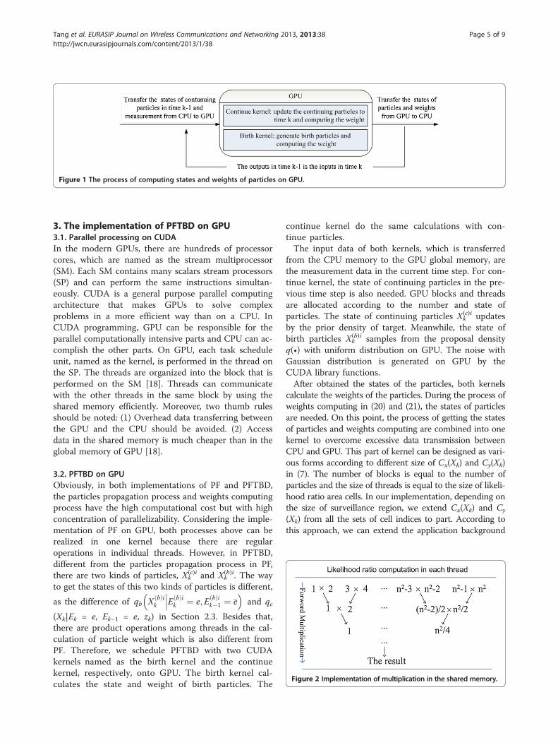
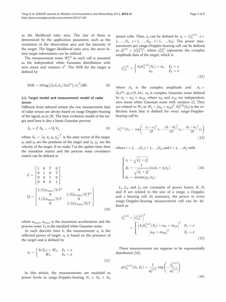
Figure 1 The process of computing states and weights of particles on GPU.

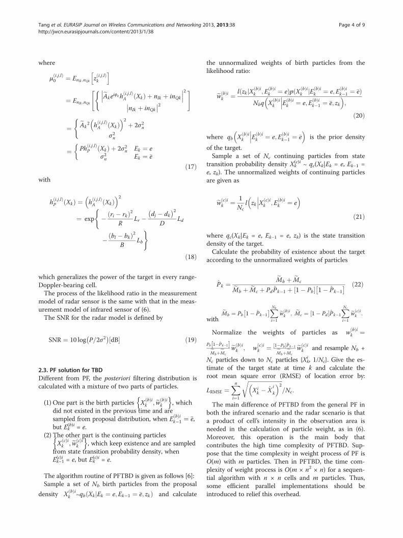
Figure 2 Implementation of multiplication in the shared memory.


3. The implementation of PFTBD on GPU3.1. Parallel processing on CUDAIn the modern GPUs, there are hundreds of processorcores, which are named as the stream multiprocessor(SM). Each SM contains many scalars stream processors(SP) and can perform the same instructions simultan-eously. CUDA is a general purpose parallel computingarchitecture that makes GPUs to solve complexproblems in a more efficient way than on a CPU. InCUDA programming, GPU can be responsible for theparallel computationally intensive parts and CPU can ac-complish the other parts. On GPU, each task scheduleunit, named as the kernel, is performed in the thread onthe SP. The threads are organized into the block that isperformed on the SM [18]. Threads can communicatewith the other threads in the same block by using theshared memory efficiently. Moreover, two thumb rulesshould be noted: (1) Overhead data transferring betweenthe GPU and the CPU should be avoided. (2) Accessdata in the shared memory is much cheaper than in theglobal memory of GPU [18].

3.2. PFTBD on GPUObviously, in both implementations of PF and PFTBD,the particles propagation process and weights computingprocess have the high computational cost but with highconcentration of parallelizability. Considering the imple-mentation of PF on GPU, both processes above can berealized in one kernel because there are regularoperations in individual threads. However, in PFTBD,different from the particles propagation process in PF,there are two kinds of particles, Xk

(c)i and Xk(b)i. The way

to get the states of this two kinds of particles is different,

as the difference of qb X bð Þik E bð Þi

k ¼ e;E bð Þik�1 ¼ �e

� and qc

(Xk|Ek = e, Ek−1 = e, zk) in Section 2.3. Besides that,there are product operations among threads in the cal-culation of particle weight which is also different fromPF. Therefore, we schedule PFTBD with two CUDAkernels named as the birth kernel and the continuekernel, respectively, onto GPU. The birth kernel cal-culates the state and weight of birth particles. The

continue kernel do the same calculations with con-tinue particles.The input data of both kernels, which is transferred

from the CPU memory to the GPU global memory, arethe measurement data in the current time step. For con-tinue kernel, the state of continuing particles in the pre-vious time step is also needed. GPU blocks and threadsare allocated according to the number and state ofparticles. The state of continuing particles Xk

(c)i updatesby the prior density of target. Meanwhile, the state ofbirth particles Xk

(b)i samples from the proposal densityq(•) with uniform distribution on GPU. The noise withGaussian distribution is generated on GPU by theCUDA library functions.After obtained the states of the particles, both kernels

calculate the weights of the particles. During the process ofweights computing in (20) and (21), the states of particlesare needed. On this point, the process of getting the statesof particles and weights computing are combined into onekernel to overcome excessive data transmission betweenCPU and GPU. This part of kernel can be designed as vari-ous forms according to different size of Cx(Xk) and Cy(Xk)in (7). The number of blocks is equal to the number ofparticles and the size of threads is equal to the size of likeli-hood ratio area cells. In our implementation, depending onthe size of surveillance region, we extend Cx(Xk) and Cy

(Xk) from all the sets of cell indices to part. According tothis approach, we can extend the application background

Figure 3 The programming on GPU for the likelihood ratio area of large scene.


from small scenes to large scenes. This problem is made afarther discussion in Section 3.3.Figure 1 shows that both kernels need current

measurements zk as the inputs. Meanwhile, to updatethe continuing particles, the previous states of continu-ing particles Xk−1

(c)i are also needed. After computing stateand weight of particles on GPU, the state and weights ofboth parts of particles, as the outputs, are transferredback to CPU.Other operations, such as calculating the probability of

detection, resampling, and estimating the state of thetarget which needs interaction for all state of particlesand their weights cannot be implemented in parallel, arearranged on CPU.

Table 1 Benchmark systems

System 1 System 2 System 3

Software Visual studio 2010 professional withCUDA 4.1 SDK

MATLAB 2010a

Hardware Nvidia GeForceGT9500

Nvidia GeForce240GT

Pentium(R) Dual-CoreE5800 @ 3.20 GHz

32 cores @ 550MHz

96 cores @ 550MHz

16.0 GB/s GDDR2 54.4 GB/s GDDR3

3.3. Likelihood ratio area programmingThe likelihood ratio function is a multiplication over allthe contributions of likelihood ratio area cells. For ascale of n2 array of likelihood ratio area cells with mparticles are used, the computing of weight will entail mblocks and resulting n2 threads in each block. The valueof n2 should be smaller than the maximum number ofthreads limited by the hardware. Under this condition,the calculating of likelihood ratio in each cell can beparallelized in every thread, but the process of productcannot be parallelized.In order to alleviate the time complexity caused by the

multiplication, the reduction algorithm is adopted in theshared memory of each block to do the product asillustrated in Figure 2. In this way, running time of themultiplication can be reduced significantly. As a result,the time complexity of weight process in PFTBD couldbe O(log2n) comparing to O(n) without using the sharedmemory.For larger application scenarios, such as in radar appli-

cation, the likelihood ratio area includes a 3D array ofdimension R × D × B, which always exceeds the max-imum available threads in one block. Thus, some strat-egies must be applied to resolve the massive parallelism

in large scene. According to the number of threads inone block, the likelihood area is divided into small areasas illustrated in Figure 3. The multiplications of eacharea A1, A2,. . .,Alast are calculated on GPU at the sametime and other areas are sequentially calculated. Thenthe result of the likelihood ratio area is the product ofall the small areas.Obviously, the operations in Figure 3 are complex.

From algorithm aspect, Torstensson and Trieb [19] havemade a research on different size of likelihood ratioareas in radar application. Its scheme is to use smalllikelihood ratio areas to obtain the tradeoff between theperformance and the extremely high computational cost.In the GPU implementation, we can follow the idea of[19] to sidestep the complex operations discussed above.More specifically, by using likelihood ratio areas withsizes that are just lower than the block, we can obtainbetter performance but with little computational cost in-crease. The simulations on different size of likelihoodratio areas are given in Section 4.2.

4. Simulation results4.1. Simulations in infrared scenarioThe simulation in infrared scenario is based on themodel in [7]. The length of observation time is 30 and atarget presents from frames 7 to 21. The observationarea is divided into n × m = 20 × 20 cells and the cellsize is Δx = Δ = 1. The probability of birth and death is

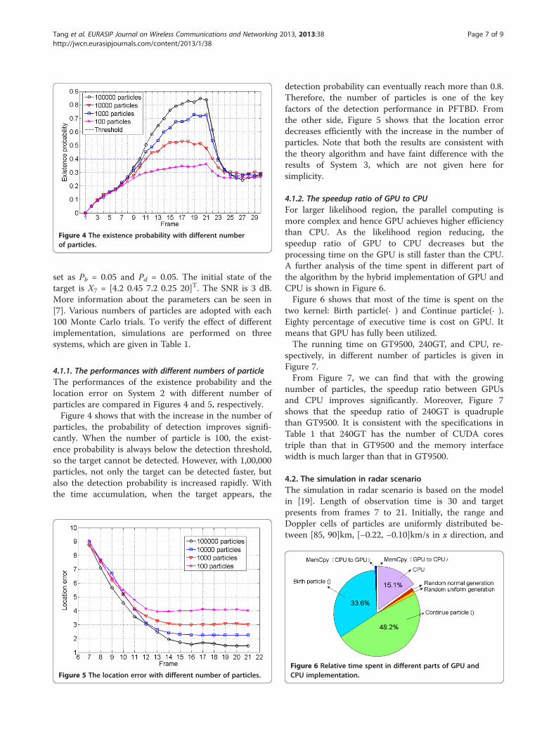
Figure 4 The existence probability with different numberof particles.


set as Pb = 0.05 and Pd = 0.05. The initial state of thetarget is X7 = [4.2 0.45 7.2 0.25 20]T. The SNR is 3 dB.More information about the parameters can be seen in[7]. Various numbers of particles are adopted with each100 Monte Carlo trials. To verify the effect of differentimplementation, simulations are performed on threesystems, which are given in Table 1.

4.1.1. The performances with different numbers of particleThe performances of the existence probability and thelocation error on System 2 with different number ofparticles are compared in Figures 4 and 5, respectively.Figure 4 shows that with the increase in the number of

particles, the probability of detection improves signifi-cantly. When the number of particle is 100, the exist-ence probability is always below the detection threshold,so the target cannot be detected. However, with 1,00,000particles, not only the target can be detected faster, butalso the detection probability is increased rapidly. Withthe time accumulation, when the target appears, the

Figure 5 The location error with different number of particles.

detection probability can eventually reach more than 0.8.Therefore, the number of particles is one of the keyfactors of the detection performance in PFTBD. Fromthe other side, Figure 5 shows that the location errordecreases efficiently with the increase in the number ofparticles. Note that both the results are consistent withthe theory algorithm and have faint difference with theresults of System 3, which are not given here forsimplicity.

4.1.2. The speedup ratio of GPU to CPUFor larger likelihood region, the parallel computing ismore complex and hence GPU achieves higher efficiencythan CPU. As the likelihood region reducing, thespeedup ratio of GPU to CPU decreases but theprocessing time on the GPU is still faster than the CPU.A further analysis of the time spent in different part ofthe algorithm by the hybrid implementation of GPU andCPU is shown in Figure 6.Figure 6 shows that most of the time is spent on the

two kernel: Birth particle(∙ ) and Continue particle(∙ ).Eighty percentage of executive time is cost on GPU. Itmeans that GPU has fully been utilized.The running time on GT9500, 240GT, and CPU, re-

spectively, in different number of particles is given inFigure 7.From Figure 7, we can find that with the growing

number of particles, the speedup ratio between GPUsand CPU improves significantly. Moreover, Figure 7shows that the speedup ratio of 240GT is quadruplethan GT9500. It is consistent with the specifications inTable 1 that 240GT has the number of CUDA corestriple than that in GT9500 and the memory interfacewidth is much larger than that in GT9500.

4.2. The simulation in radar scenarioThe simulation in radar scenario is based on the modelin [19]. Length of observation time is 30 and targetpresents from frames 7 to 21. Initially, the range andDoppler cells of particles are uniformly distributed be-tween [85, 90]km, [−0.22, −0.10]km/s in x direction, and

Figure 6 Relative time spent in different parts of GPU andCPU implementation.

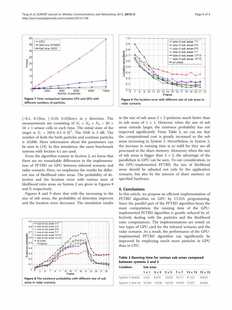
Figure 9 The location error with different size of sub areas inradar scenario.

Figure 7 Time comparison between CPU and GPU withdifferent numbers of particles.


[−0.1, 0.1]km, [−0.10, 0.10]km/s in y direction. Themeasurements are consisting of Nr × Nd × Nb = 50 ×16 × 1 sensor cells in each time. The initial state of thetarget is X7 = [89.6 0.2 0 0]T. The SNR is 3 dB. Thenumber of both the birth particles and continue particlesis 10,000. More information about the parameters canbe seen in [19]. In this simulation, the same benchmarksystems with Section 4.1 are used.From the algorithm routine in Section 2, we know that

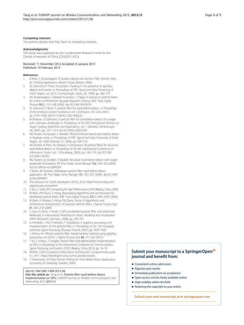
there are no remarkable differences in the implementa-tion of PFTBD on GPU between infrared scenario andradar scenario. Here, we emphasize the results for differ-ent size of likelihood ratio areas. The probability of de-tection and the location error with various sizes oflikelihood ratio areas on System 2 are given in Figures 8and 9, respectively.Figures 8 and 9 show that with the increasing in the

size of sub areas, the probability of detection improvesand the location error decreases. The simulation results

Figure 8 The existence probability with different size of subareas in radar scenario.

in the size of sub areas 3 × 3 performs much better thanin sub areas of 1 × 1. However, when the size of subareas extends larger, the existence probability has notimproved significantly. From Table 2, we can see thatthe computational cost is greatly increased as the subareas increasing in System 3. Nevertheless, in System 2,the increase in running time is so mild for they are allprocessed in the share memory. Moreover, when the sizeof sub areas is bigger than 5 × 5, the advantage of theparallelism in GPU can be seen. To our consideration, inthe GPU-implemented PFTBD, the size of likelihoodareas should be adjusted not only by the applicationscenario, but also by the amount of share memory onspecified hardware.

5. ConclusionsIn this article, we propose an efficient implementation ofPFTBD algorithm on GPU by CUDA programming.Since the parallel part of the PFTBD algorithm bears themain computation, the running time of the GPU-implemented PFTBD algorithm is greatly reduced by ef-fectively dealing with the particles and the likelihoodratio computations. The implementations are tested ontwo types of GPU card for the infrared scenario and theradar scenario. As a result, the performance of the GPU-implemented PFTBD algorithm can significantly beimproved by employing much more particles in GPUthan in CPU.

Table 2 Running time for various sub areas comparedbetween systems 2 and 3

Condition Sub areas

1 × 1 3 × 3 5 × 5 7 × 7 13 × 13 15 × 15

System 3 time(s) 3.422 6.070 10.025 16.171 41.322 50.853

System 2 time (s) 10.343 10.436 10.578 10.976 15.972 20.446


Competing interestsThe authors declare that they have no competing interests.

AcknowledgmentsThis study was supported by the Fundamental Research Funds for theCentral Universities of China (ZYGX2011J012).

Received: 11 December 2012 Accepted: 8 January 2013Published: 19 February 2013

References1. B Ristic, S Arulampalam, N Gordon, Beyond the Kalman Filter: Particle Filters,

for Tracking Applications (Artech House, Boston, 2004)2. DJ Salmond, D Fisher, NJ Gordon, Tracking in the presence of spurious

objects and clutter, in Proceedings of SPIE, Signal and Data Processing ofSmall Targets, vol. 3373 (, Farnborough, Hants, UK, 1998), pp. 460–747

3. MS Arulampalam, S Maskell, N Gordon, T Clapp, A tutorial on particle filtersfor online nonlinear/non-Gaussian Bayesian tracking. IEEE Trans SignalProcess 50(2), 174–188 (2002). doi:10.1109/78.978374

4. DJ Salmond, H Birch, A particle filter for track-before-detect, in Proceedingsof the American Control Conference. vol. 5 (Arlington, VA, USA, 2001),pp. 3755–3760. doi:10.1109/ACC.2001.946220

5. M Rollason, D Salmond, A particle filter for track-before-detect of a targetwith unknown amplitude, in Proceedings of the IEEE International Seminar onTarget Tracking Algorithms and Applications. vol. 1 (QinetiQ, Farnborough,UK, 2001), pp. 14-1–14-4. doi:10.1049/ic:20010240

6. MG Rutten, NJ Gordon, S Maskell, Efficient Particle based track before detectin Rayleigh noise, in Proceedings of SPIE, Signal and Data Processing of SmallTargets, vol. 5428 (Orlando, FL, 2004), pp. 509–519

7. MG Rutten, B Ristic, NJ Gredon, A comparison of particle filters for recursivetrack-before-detect, in Proceedings of the 8th International Conference onInformation Fusion. vol. 1 (Piscataway, 2005), pp. 169–175. doi:10.1109/ICIF.2005.1591851

8. MG Rutten, NJ Gordon, S Maskell, Recursive track-before-detect with targetamplitude fluctuations. IEE Proc Radar Sonar Navigat 152, 345–352 (2005).doi:10.1049/ip-rsn:20045041

9. Y Boers, JN Driessen, Multitarget particle filter track before detectapplication. IEE Proc Radar Sonar Navigat 151, 351–357 (2004). doi:10.1049/ip-rsn:20040841

10. The resource for CUDA developers (2010), 2010. http://www.nvidia.com/object/cuda_home.html

11. Z Shu, C Yanli, GPU Computing for High Performance-CUDA (Beijing, China, 2009)12. M Bolic, PM Djuric, S Hong, Resampling algorithms and architectures for

distributed particle filters. IEEE Trans Signal Process 53(7), 2442–2450 (2005)13. M Bolic, A Athalye, S Hong, PM Djuric, Study of algorithmic and

architectural characteristics of Gaussian particle filters. J Signal Process Syst61, 205–218 (2009)

14. C Lenz, G Panin, A Knoll, A GPU-accelerated particle filter with pixel-levellikelihood, in International Workshop on Vision, Modeling and Visualization(VMV) (Konstanz, Germany, 2008), pp. 235–241

15. G Hendeby, J Hol, R Karlsson, F Gustafsson, A graphics processing unitimplementation of the particle filter, in Proceedings of the 15th EuropeanStatistical Signal Processing (Poznan, Poland, 2007), pp. 1639–1643

16. L Peihua, An efficient particle filter–based tracking method using graphicsprocessing unit (GPU). J Signal Process Syst 68, 317–332 (2012)

17. T Xu, S Jinzhou, Z Fangbin, Particle filter track-before-detect implementationon GPU, in Proceedings of the International Conference on Communications,Signal Processing, and Systems (CSPS) (Beijing, China, 2012), pp. 16–18

18. NVIDIA, CUDA (Compute Unified Device Architecture) C programming guide4.1, 2011. https://developer.nvidia.com/cuda-downloads

19. J Torstensson, M Trieb, Particle Filtering for Track Before Detect Applications(University of Linkoping, Sweden, 2005)

doi:10.1186/1687-1499-2013-38Cite this article as: Tang et al.: Particle filter track-before-detectimplementation on GPU. EURASIP Journal on Wireless Communications andNetworking 2013 2013:38.

Submit your manuscript to a journal and benefi t from:

7 Convenient online submission

7 Rigorous peer review

7 Immediate publication on acceptance

7 Open access: articles freely available online

7 High visibility within the fi eld

7 Retaining the copyright to your article

Submit your next manuscript at 7 springeropen.com

http://dx.doi.org/10.1109/78.978374

http://dx.doi.org/10.1109/ACC.2001.946220

http://dx.doi.org/10.1049/ic:20010240

http://dx.doi.org/10.1109/ICIF.2005.1591851

http://dx.doi.org/10.1109/ICIF.2005.1591851

http://dx.doi.org/10.1049/ip-rsn:20045041



http://www.nvidia.com/object/cuda_home.html

http://www.nvidia.com/object/cuda_home.html

https://developer.nvidia.com/cuda-downloads

Documents

RESEARCH Open Access Particle filter track-before-detect