a SpringerOpen Journal

Thukral SpringerPlus 2014, 3:658http://www.springerplus.com/content/3/1/658

RESEARCH Open Access

Factorials of real negative and imaginarynumbers - A new perspectiveAshwani K Thukral

Abstract

Presently, factorials of real negative numbers and imaginary numbers, except for zero and negative integers areinterpolated using the Euler’s gamma function. In the present paper, the concept of factorials has been generalisedas applicable to real and imaginary numbers, and multifactorials. New functions based on Euler’s factorial functionhave been proposed for the factorials of real negative and imaginary numbers. As per the present concept, thefactorials of real negative numbers, are complex numbers. The factorials of real negative integers have theirimaginary part equal to zero, thus are real numbers. Similarly, the factorials of imaginary numbers are complexnumbers. The moduli of the complex factorials of real negative numbers, and imaginary numbers are equal to theirrespective real positive number factorials. Fractional factorials and multifactorials have been defined in a newperspective. The proposed concept has also been extended to Euler’s gamma function for real negative numbersand imaginary numbers, and beta function.

Keywords: Factorials of negative numbers; Factorials of imaginary numbers; Pi function; Fractional factorials;Multifactorials; Gamma function; Beta function

BackgroundThe factorial of a positive integer, n, is defined as,

n! ¼ 1:2:3 :::: n−1ð Þ nð Þ ¼ Πn

k¼1k;

0! ¼ 1

The factorials of positive integers follow the recur-rence relation,

n! ¼ n n−1ð Þ!; n≥1The factorials of negative integers cannot be com-

puted, since for n = 0, the recurrence relation,

n−1ð Þ! ¼ n!n;

involves a division by zero. Research on the interpolationof factorials started with correspondence among LeonhardEuler, Daniel Bernoulli and Christian Goldbach in theyear 1729 (Refer to the correspondence reproduced byDartmouth College 2014; and Luschny 2014a). Bernoulli

Correspondence: akthukral.gndu@gmail.comDepartment of Botanical & Environmental Sciences, Guru Nanak DevUniversity, Amritsar 143005, India

© 2014 Thukral; licensee Springer. This is an OpAttribution License (http://creativecommons.orin any medium, provided the original work is p

in the year 1729 gave an interpolating function of facto-rials as an infinite product (Gronau 2003). Euler in theyear 1730 proved that the integral,

x! ¼ Π xð Þ ¼Z10

− lntð Þxdt ¼Z∞

0

txe−tdt; x > −1; ð1Þ

gives the factorial of x for all real positive numbers(Srinivasan 2007). Euler’s factorial function, also knownas the Pi function, Π(x), follows the recurrence relationfor all positive real numbers.

Π xþ 1ð Þ ¼ xþ 1ð ÞΠ xð Þ; x≥0In 1768, Euler defined the gamma function, Γ(z), and

extended the concept of factorials to all real negativenumbers, except zero and negative integers. Γ(z), is anextension of the Pi function, with its argument shifteddown by 1. Also known as the Euler’s integral of the sec-ond kind (Gautschi 2008), it is a convergent improperintegral defined as follows:

Γ zð Þ ¼Z∞

0

tz−1e−tdt ð2Þ

en Access article distributed under the terms of the Creative Commonsg/licenses/by/4.0), which permits unrestricted use, distribution, and reproductionroperly credited.

Thukral SpringerPlus 2014, 3:658 Page 2 of 13http://www.springerplus.com/content/3/1/658

The Euler’s gamma function is related to the Pi func-tion as follows:

Π xð Þ ¼ Γ xþ 1ð Þ ¼ x!

The notation ‘!’ for the factorial function was intro-duced by C. Kramp in the year 1808 (Wolfram Research2014a,b). Legendre in 1808 gave the notation ‘Γ’ to theEuler’s gamma function (Gronau 2003). Gauss intro-duced the notation

Π sð Þ ¼ Γ sþ 1ð Þ;

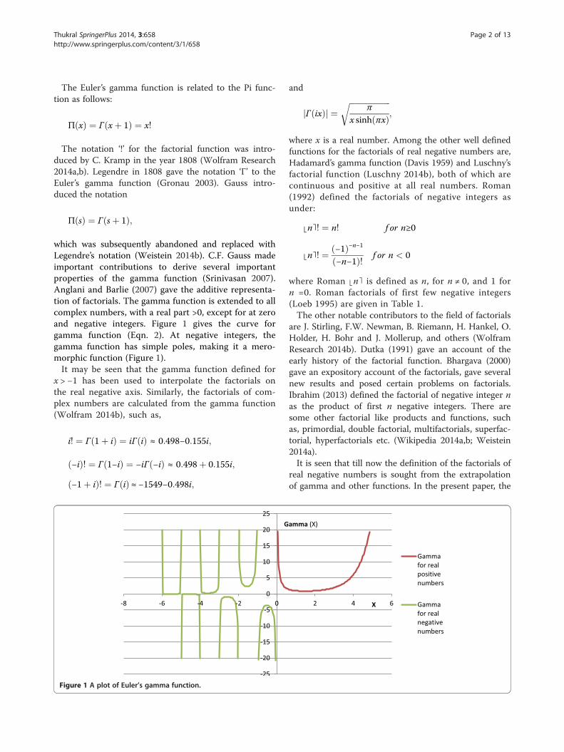
which was subsequently abandoned and replaced withLegendre’s notation (Weistein 2014b). C.F. Gauss madeimportant contributions to derive several importantproperties of the gamma function (Srinivasan 2007).Anglani and Barlie (2007) gave the additive representa-tion of factorials. The gamma function is extended to allcomplex numbers, with a real part >0, except for at zeroand negative integers. Figure 1 gives the curve forgamma function (Eqn. 2). At negative integers, thegamma function has simple poles, making it a mero-morphic function (Figure 1).It may be seen that the gamma function defined for

x > −1 has been used to interpolate the factorials onthe real negative axis. Similarly, the factorials of com-plex numbers are calculated from the gamma function(Wolfram 2014b), such as,

i! ¼ Γ 1þ ið Þ ¼ iΓ ið Þ ≈ 0:498−0:155i;

−ið Þ! ¼ Γ 1−ið Þ ¼ −iΓ −ið Þ ≈ 0:498þ 0:155i;

−1þ ið Þ! ¼ Γ ið Þ ≈ −1549−0:498i;

Figure 1 A plot of Euler’s gamma function.

and

ffiffiffiffiffiffiffiffiffiffiffiffiffiffiffiffiffiffiffiffiffir

Γ ixð Þj j ¼ π

x sinh πxð Þ;

where x is a real number. Among the other well definedfunctions for the factorials of real negative numbers are,Hadamard’s gamma function (Davis 1959) and Luschny’sfactorial function (Luschny 2014b), both of which arecontinuous and positive at all real numbers. Roman(1992) defined the factorials of negative integers asunder:

⌊n⌉! ¼ n! f or n≥0

⌊n⌉! ¼ −1ð Þ−n−1−n−1ð Þ! f or n < 0

where Roman ⌊n⌉ is defined as n, for n ≠ 0, and 1 forn =0. Roman factorials of first few negative integers(Loeb 1995) are given in Table 1.The other notable contributors to the field of factorials

are J. Stirling, F.W. Newman, B. Riemann, H. Hankel, O.Holder, H. Bohr and J. Mollerup, and others (WolframResearch 2014b). Dutka (1991) gave an account of theearly history of the factorial function. Bhargava (2000)gave an expository account of the factorials, gave severalnew results and posed certain problems on factorials.Ibrahim (2013) defined the factorial of negative integer nas the product of first n negative integers. There aresome other factorial like products and functions, suchas, primordial, double factorial, multifactorials, superfac-torial, hyperfactorials etc. (Wikipedia 2014a,b; Weistein2014a).It is seen that till now the definition of the factorials of

real negative numbers is sought from the extrapolationof gamma and other functions. In the present paper, the

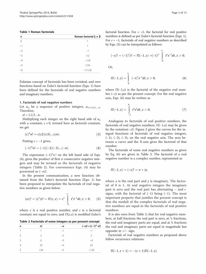
Table 1 Roman factorials

n Roman factorial ⌊ n ⌉!

0 1

−1 1

−2 −1

−3 1/2

−4 −1/6

−5 1/24

−6 −1/120

Thukral SpringerPlus 2014, 3:658 Page 3 of 13http://www.springerplus.com/content/3/1/658

Eularian concept of factorials has been revisited, and newfunctions based on Euler’s factorial function (Eqn. 1) havebeen defined for the factorials of real negative numbersand imaginary numbers.

1. Factorials of real negative numbersLet an be a sequence of positive integers, an=1,2,3,…,n.

Therefore,n! = 1.2.3…n.Multiplying each integer on the right hand side of an

with a constant, c ≠ 0, termed here as factorial constant,we get

cð Þnn! ¼ c c2ð Þ c3ð Þ… cnð Þ: ð3ÞPutting c = −1 gives,

−1ð Þnn! ¼ −1ð Þ −2ð Þ −3ð Þ… −nð Þ: ð4ÞThe expression (−1)nn ! on the left hand side of Eqn.

(4), gives the product of first n consecutive negative inte-gers and may be termed as the factorials of negativeintegers (Table 2). For convenience Eqn. (4) may bepresented as (−n)!.In the present communication, a new function ob-

tained from the Euler’s factorial function (Eqn. 1) hasbeen proposed to interpolate the factorials of real nega-tive numbers as given below:

czð Þ! ¼ czð Þz! ¼ Π c; zð Þ ¼ czZ∞

0

tze−tdt; z > 0; ð5Þ

where z is a real positive number, and c is a factorialconstant not equal to zero, and Π(c,z) is modified Euler’s

Table 2 Factorials of some integers as per present concept

n n! −n (−n)! = [(−1)n n!]

1 1 −1 −1

2 2 −2 2

3 6 −3 −6

4 24 −4 24

5 120 −5 −120

factorial function. For c =1, the factorial for real positivenumbers is defined as per Euler’s factorial function (Eqn. 1).For c = −1, factorials of real negative numbers as describedby Eqn. (5) can be interpolated as follows:

−zð Þ! ¼ −1ð Þzz! ¼ Π −1; zð Þ ¼ −1ð ÞzZ∞

0

tze−tdt; z > 0;

Or,

Π −1; zð Þ ¼Z∞

0

−tð Þze−tdt; z > 0; ð6Þ

where Π(−1,z) is the factorial of the negative real num-ber (−z) as per the present concept. For the real negativeaxis, Eqn. (6) may be written as

Π −1; zð Þ ¼Z0−∞

tzetdt; z > 0: ð7Þ

Analogous to factorials of real positive numbers, thefactorials of real negative numbers, Π(−1,z) may be givenby the notation(−z)!. Figure 2 gives the curves for the in-tegral functions of factorials of real negative integers,(−1), (−2), (−3), on the real negative axis. The area be-tween a curve and the X-axis gives the factorial of thatnumber.The factorials of some real negative numbers as given

by Eq. (6) are given in Table 3. The factorial of a realnegative number is a complex number, represented as

Π −1; zð Þ ¼ −zð Þ! ¼ xþ iy;

where x is the real part and y is imaginary. The factor-ial of 0 is 1. At real negative integers the imaginarypart is zero and the real part has alternating – and +signs, with the factorial of (−1) being (−1). The mostimportant property that justifies the present concept isthat the moduli of the complex factorials of real nega-tive numbers are equal to the factorials of real positivenumbers.It is also seen from Table 3, that for real negative num-

bers, at half fractions the real part is zero, at ¼ fractions,the real and imaginary parts are equal, and at ¾ fractionsthe real and imaginary parts are equal in magnitude butopposite in +/− sign.Factorials of real negative numbers as proposed above

follow recurrence relations:

Π −1; z þ 1ð Þ ¼ − z þ 1ð ÞΠ −1; zð Þ:

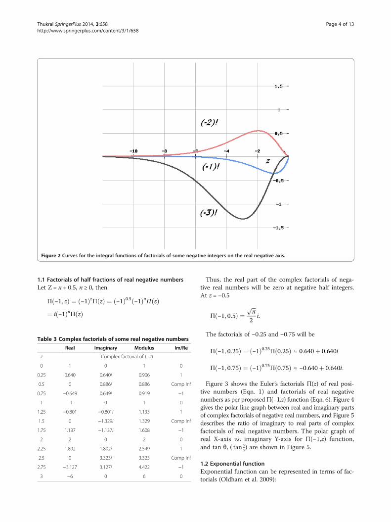
Figure 2 Curves for the integral functions of factorials of some negative integers on the real negative axis.

Thukral SpringerPlus 2014, 3:658 Page 4 of 13http://www.springerplus.com/content/3/1/658

1.1 Factorials of half fractions of real negative numbersLet Z = n + 0.5, n ≥ 0, then

Π −1; zð Þ ¼ −1ð ÞzΠ zð Þ ¼ −1ð Þ0:5 −1ð ÞnΠ zð Þ¼ i −1ð ÞnΠ zð Þ

Table 3 Complex factorials of some real negative numbers

Real Imaginary Modulus Im/Re

z Complex factorial of (−z)

0 1 0 1 0

0.25 0.640 0.640i 0.906 1

0.5 0 0.886i 0.886 Comp Inf

0.75 −0.649 0.649i 0.919 −1

1 −1 0 1 0

1.25 −0.801 −0.801i 1.133 1

1.5 0 −1.329i 1.329 Comp Inf

1.75 1.137 −1.137i 1.608 −1

2 2 0 2 0

2.25 1.802 1.802i 2.549 1

2.5 0 3.323i 3.323 Comp Inf

2.75 −3.127 3.127i 4.422 −1

3 −6 0 6 0

Thus, the real part of the complex factorials of nega-tive real numbers will be zero at negative half integers.At z = −0.5

Π −1; 0:5ð Þ ¼ffiffiffiπ

p2

i:

The factorials of −0.25 and −0.75 will be

Π −1; 0:25ð Þ ¼ −1ð Þ0:25Π 0:25ð Þ ≈ 0:640þ 0:640i

Π −1; 0:75ð Þ ¼ −1ð Þ0:75Π 0:75ð Þ ≈ −0:640þ 0:640i:

Figure 3 shows the Euler’s factorials Π(z) of real posi-tive numbers (Eqn. 1) and factorials of real negativenumbers as per proposedΠ(−1,z) function (Eqn. 6). Figure 4gives the polar line graph between real and imaginary partsof complex factorials of negative real numbers, and Figure 5describes the ratio of imaginary to real parts of complexfactorials of real negative numbers. The polar graph ofreal X-axis vs. imaginary Y-axis for Π(−1,z) function,and tan θ, ( tan y

x) are shown in Figure 5.

1.2 Exponential functionExponential function can be represented in terms of fac-torials (Oldham et al. 2009):

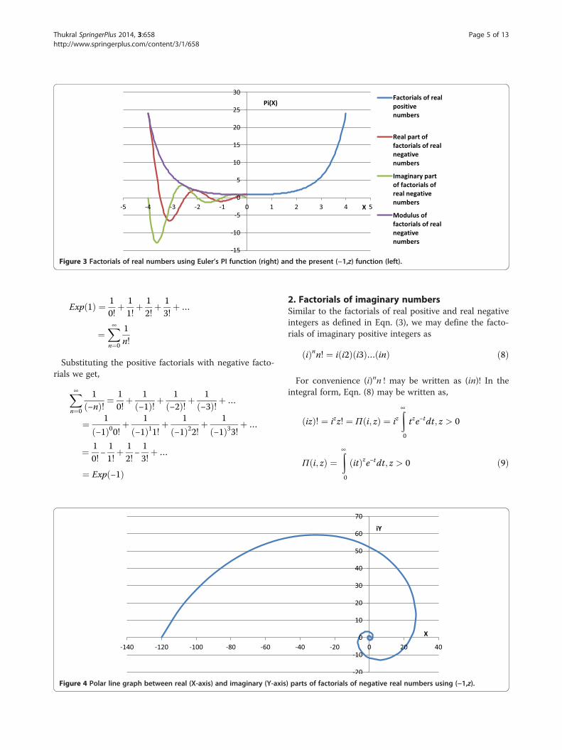
Figure 3 Factorials of real numbers using Euler’s PI function (right) and the present (−1,z) function (left).

Thukral SpringerPlus 2014, 3:658 Page 5 of 13http://www.springerplus.com/content/3/1/658

Exp 1ð Þ ¼ 10!þ 11!þ 12!þ 13!þ…

¼X∞n¼0

1n!

Substituting the positive factorials with negative facto-rials we get,

X∞n¼0

1−nð Þ! ¼

10!þ 1

−1ð Þ!þ1−2ð Þ!þ

1−3ð Þ!þ…

¼ 1

−1ð Þ00!þ1

−1ð Þ11!þ1

−1ð Þ22!þ1

−1ð Þ33!þ…

¼ 10!−11!þ 12!−13!þ…

¼ Exp −1ð Þ

Figure 4 Polar line graph between real (X-axis) and imaginary (Y-axis

2. Factorials of imaginary numbersSimilar to the factorials of real positive and real negativeintegers as defined in Eqn. (3), we may define the facto-rials of imaginary positive integers as

ið Þnn! ¼ i i2ð Þ i3ð Þ… inð Þ ð8Þ

For convenience (i)nn ! may be written as (in)! In theintegral form, Eqn. (8) may be written as,

izð Þ! ¼ izz! ¼ Π i; zð Þ ¼ izZ∞

0

tze−tdt; z > 0

Π i; zð Þ ¼Z∞

0

itð Þze−tdt; z > 0 ð9Þ

) parts of factorials of negative real numbers using (−1,z).

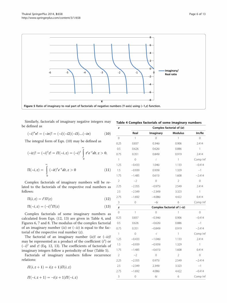
Figure 5 Ratio of imaginary to real part of factorials of negative numbers (Y-axis) using (−1,z) function.

Table 4 Complex factorials of some imaginary numbers

z Complex factorial of (iz)

Real Imaginary Modulus Im/Re

0 1 0 1 0

0.25 0.837 0.346i 0.906 2.414

0.5 0.626 0.626i 0.886 1

0.75 0.351 0.849i 0.919 2.414

1 0 i 1 Comp Inf

1.25 −0.433 1.046i 1.133 −0.414

1.5 −0.939 0.939i 1.329 −1

1.75 −1.485 0.615i 1.608 −2.414

2 −2 0 2 0

2.25 −2.355 −0.975i 2.549 2.414

2.5 −2.349 −2.349i 3.323 1

2.75 −1.692 −4.086i 4.422 0.414

3 0 −6i 6 Comp Inf

z Complex factorial of (−iz)

0 1 0 1 0

0.25 0.837 −0.346i 0.906 −0.414

0.5 0.626 −0.626i 0.886 −1

0.75 0.351 −0.849i 0.919 −2.414

1 0 -i 1 Comp Inf

1.25 −0.433 −1.046i 1.133 2.414

1.5 −0.939 −0.939i 1.329 1

1.75 −1.485 −0.615i 1.608 0.414

2 −2 0 2 0

2.25 −2.355 0.975i 2.549 −2.414

2.5 −2.349 2.349i 3.323 −1

2.75 −1.692 4.086i 4.422 −0.414

3 0 6i 6 Comp Inf

Thukral SpringerPlus 2014, 3:658 Page 6 of 13http://www.springerplus.com/content/3/1/658

Similarly, factorials of imaginary negative integers maybe defined as

−ið Þnn! ¼ −inð Þ! ¼ −ið Þ −i2ð Þ −i3ð Þ… −inð Þ ð10ÞThe integral form of Eqn. (10) may be defined as

−izð Þ! ¼ −ið Þzz! ¼ Π −i; zð Þ ¼ −ið ÞzZ∞

0

tze−tdt; z > 0;

Π −i; zð Þ ¼Z∞

0

−itð Þze−tdt; z > 0 ð11Þ

Complex factorials of imaginary numbers will be re-lated to the factorials of the respective real numbers asfollows:

Π i; zð Þ ¼ izΠ zð Þ ð12ÞΠ −i; zð Þ ¼ −ið ÞzΠ zð Þ ð13Þ

Complex factorials of some imaginary numbers ascalculated from Eqn. (12, 13) are given in Table 4, andFigures 6, 7 and 8. The modulus of the complex factorialof an imaginary number (iz) or (−iz) is equal to the fac-torial of the respective real number (z).The factorial of an imaginary number (iz)! or (−iz)!

may be represented as a product of the coefficient (iz) or(−i)z and z! (Eq. 12, 13). The coefficients of factorials ofimaginary integers follow a periodicity of four (Table 5).Factorials of imaginary numbers follow recurrence

relations:

Π i; z þ 1ð Þ ¼ i z þ 1ð ÞΠ i; zð Þ

Π −i; z þ 1ð Þ ¼ −i z þ 1ð ÞΠ −i; zð Þ

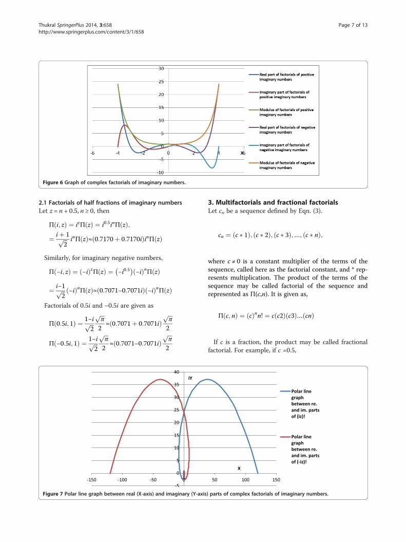
Figure 6 Graph of complex factorials of imaginary numbers.

Thukral SpringerPlus 2014, 3:658 Page 7 of 13http://www.springerplus.com/content/3/1/658

2.1 Factorials of half fractions of imaginary numbersLet z = n + 0.5, n ≥ 0, then

Π i; zð Þ ¼ izΠ zð Þ ¼ i0:5inΠ zð Þ;¼ iþ 1ffiffiffi

2p inΠ zð Þ≈ 0:7170þ 0:7170ið ÞinΠ zð Þ

Similarly, for imaginary negative numbers,

Π −i; zð Þ ¼ −ið ÞzΠ zð Þ ¼ −i0:5� �

−ið ÞnΠ zð Þ

¼ i−1ffiffiffi2

p −ið ÞnΠ zð Þ≈ 0:7071−0:7071ið Þ −ið ÞnΠ zð Þ

Factorials of 0.5i and −0.5i are given as

Π 0:5i; 1ð Þ ¼ 1−iffiffiffi2

pffiffiffiπ

p2

≈ 0:7071þ 0:7071ið Þffiffiffiπ

p2

Π −0:5i; 1ð Þ ¼ 1−iffiffiffi2

pffiffiffiπ

p2

≈ 0:7071−0:7071ið Þffiffiffiπ

p2

Figure 7 Polar line graph between real (X-axis) and imaginary (Y-axis

3. Multifactorials and fractional factorialsLet cn be a sequence defined by Eqn. (3).

cn ¼ c � 1ð Þ; c � 2ð Þ; c � 3ð Þ;…; c � nð Þ;

where c ≠ 0 is a constant multiplier of the terms of thesequence, called here as the factorial constant, and * rep-resents multiplication. The product of the terms of thesequence may be called factorial of the sequence andrepresented as Π(c,n). It is given as,

Π c; nð Þ ¼ cð Þnn! ¼ c c2ð Þ c3ð Þ… cnð Þ

If c is a fraction, the product may be called fractionalfactorial. For example, if c =0.5,

) parts of complex factorials of imaginary numbers.

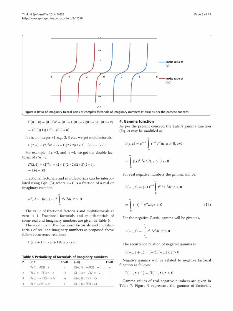
Figure 8 Ratio of imaginary to real parts of complex factorials of imaginary numbers (Y-axis) as per the present concept.

Thukral SpringerPlus 2014, 3:658 Page 8 of 13http://www.springerplus.com/content/3/1/658

Π 0:5; nð Þ ¼ 0:5ð Þnn! ¼ 0:5 � 1ð Þ 0:5 � 2ð Þ 0:5 � 3ð Þ… 0:5 � nð Þ

¼ 0:5ð Þ 1ð Þ 1:5ð Þ… 0:5 � nð ÞIf c is an integer >1, e.g., 2, 3 etc., we get multifactorials.

Π 2; nð Þ ¼ 2ð Þnn! ¼ 2 � 1ð Þ 2 � 2ð Þ 2 � 3ð Þ… 2nð Þ ¼ 2nð Þ!!

For example, if c =2, and n =4, we get the double fac-torial of c*n =8,

Π 2; 4ð Þ ¼ 2ð Þ44! ¼ 2 � 1ð Þ 2 � 2ð Þ 2 � 3ð Þ 2 � 4ð Þ;¼ 384 ¼ 8!!

Fractional factorials and multifactorials can be interpo-lated using Eqn. (5), where c ≠ 0 is a fraction of a real orimaginary number.

czð Þz! ¼ Π c; zð Þ ¼ czZ∞

0

tze−tdt; z > 0

The value of fractional factorials and multifactorials atzero is 1. Fractional factorials and multifactorials ofsome real and imaginary numbers are given in Table 6.The modulus of the fractional factorials and multifac-

torials of real and imaginary numbers as proposed abovefollow recurrence relations:

Π c; z þ 1ð Þ ¼ c z þ 1ð ÞΠ c; zð Þ; c≠0

Table 5 Periodicity of factorials of imaginary numbers

Z (iz) ! Coeff. (−iz) ! Coeff.

1 Π(i, 1) = iΠ(1) = i i Π(−i, 1) = − iΠ(1) = − i −i

2 Π(i, 2) = − Π(2) = − 2 −1 Π(−i, 2) = − Π(2) = − 2 −1

3 Π(i, 3) = − iΠ(3) = − 6i −i Π(−i, 3) = iΠ(3) = 6i i

4 Π(i, 4) = Π(4) = 24 1 Π(−i, 4) = Π(4) = 24 1

4. Gamma functionAs per the present concept, the Euler’s gamma function(Eq. 2) may be modified as,

Γ c; zð Þ ¼ cz−1Z∞

0

tz−1e−tdt; z > 0; c≠0

¼Z∞

0

ctð Þz−1e−tdt; z > 0; c≠0

For real negative numbers the gamma will be,

Γ −1; zð Þ ¼ −1ð Þz−1Z∞

0

tz−1e−tdt; z > 0

¼Z∞

0

−tð Þz−1e−tdt; z > 0 ð14Þ

For the negative Z-axis, gamma will be given as,

Γ −1; zð Þ ¼Z0−∞

tz−1etdt; z > 0

The recurrence relation of negative gamma is:

Γ −1; z þ 1ð Þ ¼ −zð ÞΓ −1; zð Þ; z > 0

Negative gamma will be related to negative factorialfunction as follows:

Γ −1; z þ 1ð Þ ¼ Π −1; zð Þ; z > 0

Gamma values of real negative numbers are given inTable 7. Figure 9 represents the gamma of factorials

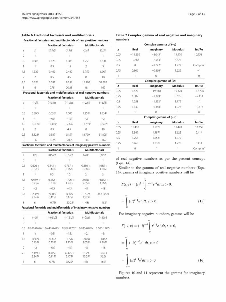
Table 6 Fractional factorials and multifactorials

Fractional factorials and multifactorials of real positive numbers

Fractional factorials Multifactorials

z z! (0.5z)! (1.5z)! (2z)!! (3z)!!!

0 1 1 1 1 1

0.5 0.886 0.626 1.085 1.253 1.534

1 1 0.5 1.5 2 3

1.5 1.329 0.469 2.442 3.759 6.907

2 2 0.5 4.5 8 18

2.5 3.323 0.587 9.158 18.799 51.805

3 6 0.75 20.25 48 162

Fractional factorials and multifactorials of real negative numbers

Fractional factorials Multifactorials

z (−z)! (−0.5)z! (−1.5z)! (−2z)!! (−3z)!!!

0 1 1 1 1 1

0.5 0.886i 0.626i 1.085 1.253i 1.534i

1 −1 −0.5 −1.5 −2 −3

1.5 −0.139i −0.469i −2.442 −3.759i −6.907i

2 2 0.5 4.5 8 18

2.5 3.323i 0.587 9.157 18.799i 51.805i

3 −6 −0.75 −20.25 −48 −162

Fractional factorials and multifactorials of imaginary positive numbers

Fractional factorials Multifactorials

z (iz!) (0.5iz)! (1.5iz)! (2iz)!! (3iz)!!!

0 1 1 1 1 1

0.5 0.626 +0.626i

0.443 +0.443i

0.767 +0.767i

0.886 +0.886i

1.085 +1.085i

1 i 0.5i 1.5i 2i 3i

1.5 −0.939 +0.939i

−0.332 +0.332i

−1.726 +1.726i

−2.658 +2.658i

−4.862 +4.862i

2 −2 −0.5 −4.5 −8 −18

2.5 −2.349-2.349i

−0.415-0.415i

−6.475-6.475i

−13.29-13.29i

36.6-36.6i

3 6i −0.75i −20.25i −48i −162i

Fractional factorials and multifactorials of imaginary negative numbers

Fractional factorials Multifactorials

z (−iz)! (−0.5iz)! (−1.5iz)! (−2iz)!! (−3iz)!!!

0 1 1 1 1 1

0.5 0.626-0.626i 0.443-0.443i 0.767-0.767i 0.886-0.886i 1.085-1.085i

1 -i −0.5i −1.5i −2i −3i

1.5 −0.939-0.939i

−0.332-0.332i

−1.726-1.726i

−2.658-2.658i

−4.862-4.862i

2 −2 −0.5 −4.5 −8 −18

2.5 −2.349 +2.349i

−0.415 +0.415i

−6.475 +6.475i

−13.29 +13.29i

−36.6 +36.6i

3 6i 0.75i 20.25i 48i 162i

Table 7 Complex gamma of real negative and imaginarynumbers

Complex gamma of (−z)

z Real Imaginary Modulus Im/Re

0.05 −19.230 −3.045i 19.470 0.158

0.25 −2.563 −2.563i 3.625 1

0.5 0 −1.772i 1.772 Comp Inf

0.75 0.866 −0.866i 1.225 −1

1 1 0 1 0

Complex gamma of (iz)

z Real Imaginary Modulus Im/Re

0.05 1.527 −19.410i 19.470 −12.706

0.25 1.387 −3.349i 3.625 −2.414

0.5 1.253 −1.253i 1.772 −1

0.75 1.132 −0.468i 1.225 −0.414

1 1 0 1 0

Complex gamma of (−iz)

z Real Imaginary Modulus Im/Re

0.05 19.410 1.527i 19.470 12.706

0.25 3.349 1.387i 3.625 2.414

0.5 1.253 1.253i 1.772 1

0.75 0.468 1.132i 1.225 0.414

1 0 i 1 Comp Inf

Thukral SpringerPlus 2014, 3:658 Page 9 of 13http://www.springerplus.com/content/3/1/658

of real negative numbers as per the present concept(Eqn. 14).Similar to the gamma of real negative numbers (Eqn.

14), gamma of imaginary positive numbers will be

Γ i; zð Þ ¼ ið Þz−1Z∞

0

tz−1e−tdt; z > 0;

¼Z∞

0

itð Þz−1e−tdt; z > 0: ð15Þ

For imaginary negative numbers, gamma will be

Γ −i; zð Þ ¼ −ið Þz−1Z∞

0

tz−1e−tdt; z > 0;

¼Z∞

0

−itð Þz−1e−tdt; z > 0

¼Z0−∞

itð Þz−1etdt; z > 0 ð16Þ

Figures 10 and 11 represent the gamma for imaginarynumbers.

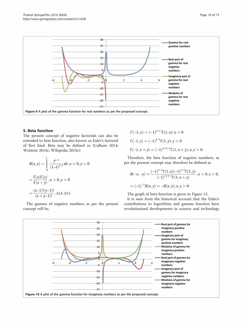
Figure 9 A plot of the gamma function for real numbers as per the proposed concept.

Thukral SpringerPlus 2014, 3:658 Page 10 of 13http://www.springerplus.com/content/3/1/658

5. Beta functionThe present concept of negative factorials can also beextended to beta function, also known as Euler’s factorialof first kind. Beta may be defined as (Culham 2014;Weistein 2014c; Wikipedia 2014c):

Β x; yð Þ ¼Z1

0

tx−1

1−tð Þy−1 dt; x > 0; y > 0

¼ Γ xð ÞΓ yð ÞΓ xþ yð Þ ; x > 0; y > 0

¼ x−1ð Þ! y−1ð Þ!xþ y−1ð Þ! ; x≥1; y≥1:

The gamma of negative numbers as per the presentconcept will be,

Figure 10 A plot of the gamma function for imaginary numbers as pe

Γ −1; xð Þ ¼ −1ð Þx−1‘Γ 1; xð Þ; x > 0

Γ −1; yð Þ ¼ −1ð Þy−1Γ 1; yð Þ; y > 0

Γ −1; xþ yð Þ ¼ −1ð Þxþy−1Γ 1; xþ yð Þ; x; y > 0:

Therefore, the beta function of negative numbers, asper the present concept may therefore be defined as

Β −x;−yð Þ ¼ −1ð Þx−1Γ 1; xð Þ −1ð Þy−1Γ 1; yð Þ−1ð Þxþy−1Γ 1; xþ yð Þ ; x > 0; y > 0;

¼ −1ð Þ−1Β x; yð Þ ¼ −Β x; yð Þ; x; y > 0:

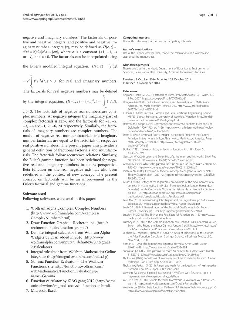
The graph of beta function is given in Figure 12.It is seen from the historical account that the Euler’s

contributions to logarithms and gamma function haverevolutionized developments in science and technology

r the proposed concept.

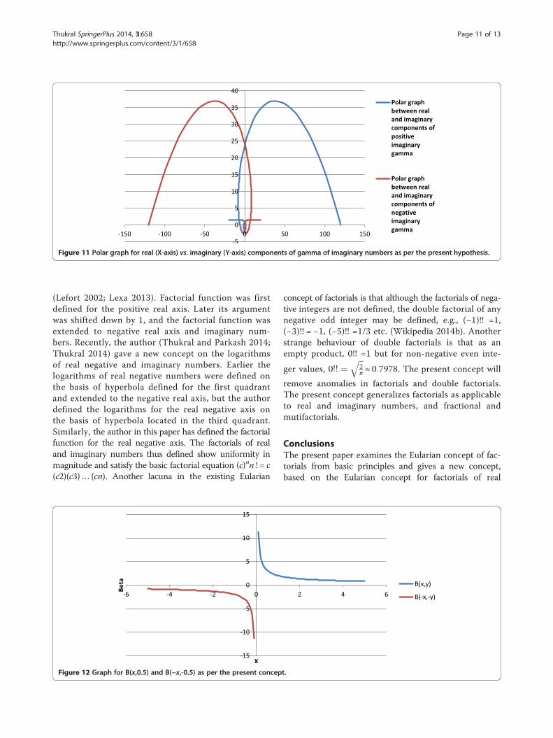
Figure 11 Polar graph for real (X-axis) vs. imaginary (Y-axis) components of gamma of imaginary numbers as per the present hypothesis.

Thukral SpringerPlus 2014, 3:658 Page 11 of 13http://www.springerplus.com/content/3/1/658

(Lefort 2002; Lexa 2013). Factorial function was firstdefined for the positive real axis. Later its argumentwas shifted down by 1, and the factorial function wasextended to negative real axis and imaginary num-bers. Recently, the author (Thukral and Parkash 2014;Thukral 2014) gave a new concept on the logarithmsof real negative and imaginary numbers. Earlier thelogarithms of real negative numbers were defined onthe basis of hyperbola defined for the first quadrantand extended to the negative real axis, but the authordefined the logarithms for the real negative axis onthe basis of hyperbola located in the third quadrant.Similarly, the author in this paper has defined the factorialfunction for the real negative axis. The factorials of realand imaginary numbers thus defined show uniformity inmagnitude and satisfy the basic factorial equation (c)nn ! = c(c2)(c3)… (cn). Another lacuna in the existing Eularian

Figure 12 Graph for B(x,0.5) and B(−x,-0.5) as per the present concep

concept of factorials is that although the factorials of nega-tive integers are not defined, the double factorial of anynegative odd integer may be defined, e.g., (−1)!! =1,(−3)!! = −1, (−5)!! =1/3 etc. (Wikipedia 2014b). Anotherstrange behaviour of double factorials is that as anempty product, 0!! =1 but for non-negative even inte-

ger values, 0!! ¼ffiffiffi2π

q≈ 0:7978. The present concept will

remove anomalies in factorials and double factorials.The present concept generalizes factorials as applicableto real and imaginary numbers, and fractional andmutifactorials.

ConclusionsThe present paper examines the Eularian concept of fac-torials from basic principles and gives a new concept,based on the Eularian concept for factorials of real

t.

Thukral SpringerPlus 2014, 3:658 Page 12 of 13http://www.springerplus.com/content/3/1/658

negative and imaginary numbers. The factorials of posi-tive and negative integers, and positive and negative im-aginary number integers (z), may be defined as Π(c, z) =czz ! = c(c2)(c3)… (cn), where c is a constant (+1, −1, +ior –i), and z >0. The factorials can be interpolated using

the Euler’s modified integral equation, Π c; zð Þ ¼ czð Þz!

¼ czZ∞

0

tze−tdt; z > 0 for real and imaginary numbers.

The factorials for real negative numbers may be defined

by the integral equation, Π −1; zð Þ ¼ −1ð Þzz! ¼Z0−∞

tzetdt;

z > 0. The factorials of negative real numbers are com-plex numbers. At negative integers the imaginary part ofcomplex factorials is zero, and the factorials for −1, −2,−3, −4 are −1, 2, −6, 24 respectively. Similarly, the facto-rials of imaginary numbers are complex numbers. Themoduli of negative real number factorials and imaginarynumber factorials are equal to the factorials of respectivereal positive numbers. The present paper also provides ageneral definition of fractional factorials and multifacto-rials. The factorials follow recurrence relations. Similarly,the Euler’s gamma function has been redefined for nega-tive real and imaginary numbers in a new perspective.Beta function on the real negative axis has also beenredefined in the context of new concept. The presentconcept on factorials will be an improvement in theEuler’s factorial and gamma functions.

Software usedFollowing softwares were used in this paper:

1. Wolfram Alpha Examples: Complex Numbers(http://www.wolframalpha.com/examples/ComplexNumbers.html)

2. Draw Function Graphs – Recheronline. (http://rechneronline.de/function-graphs/)

3. Definite integral calculator from Wolfram AlphaWidgets by Evan added in 2010 (http://www.wolframalpha.com/input/?i=definite%20integral%20calculator)

4. Integral calculator from Wolfram Mathematica Onlineintegrator (http://integrals.wolfram.com/index.jsp)

5. Gamma Function Evaluator – The WolframFunctions site http://functions.wolfram.com/webMathematica/FunctionEvaluation.jsp?name=Gamma

6. Function calculator by XIAO gang 2012 (http://wims.unice.fr/wims/en_tool~analysis~function.en.html)

7. Microsoft Excel.

Competing interestsThe author declares that he has no competing interests.

Author’s contributionsThe author conceived the idea, made the calculations and written andapproved the manuscript.

AcknowledgementsThanks are due to the Head, Department of Botanical & EnvironmentalSciences, Guru Nanak Dev University, Amritsar, for research facilities.

Received: 8 October 2014 Accepted: 23 October 2014Published: 6 November 2014

ReferencesAnglani R, Barlie M (2007) Factorials as Sums. arXiv:Math/0702010v1 [Math.HO].

1 Feb 2007. http://arxiv.org/pdf/math/0702010.pdfBhargava M (2000) The Factorial Function and Generalizations. Math. Assoc.

America. Am. Math. Monthly. 107:783–799. http://www.jstor.org/stable/2695734?origin=JSTOR-pdf

Culham JR (2014) Factorial, Gamma and Beta Functions. Engineering CourseME755- Special Functions. University of Waterloo, Waterloo. http://mhtlab.uwaterloo.ca/courses/me755/web_chap1.pdf

Dartmouth College (2014) Correspondance Between Leonhard Euler and Chr.Goldbach, 1729–1763, pp 1–59. https://www.math.dartmouth.edu/~euler/correspondence/fuss/goldbach1-59

Davis PJ (1959) Leonhard Euler’s Integral: A Historical Profile of the GammaFunction. In Memorium: Milton Abramowitz. Math. Assoc. America. AmerMath Monthly. 66:849–869. http://www.jstor.org/stable/2309786?origin=JSTOR-pdf

Dutka J (1991) The early history of factorial function. Arch Hist Exact Sci43(3):225–249

Gautschi W (2008) Leonhard Euler: His Life, the man, and his works. SIAM Rev50(1):3–33. http://www.euler-2007.ch/doc/EulerLec.pdf

Gronau D (2003) Why is the gamma function so as it is? Teach Math Comput Sci1:43–53. http://www.uni-graz.at/~gronau/TMCS_1_2003.pdf\

Ibrahim AM (2013) Extension of factorial concept to negative numbers. NotesTheory Discrete Math 19:30–42. http://nntdm.net/papers/nntdm-19/NNTDM-19-2-30_42.pdf

Lefort X (2002) History of the logarithms: an example of the development of aconcept in mathematics. (In: Project Penelope, editor: Miguel HernandezGonzalez) Fundaciõn Canaria Orotava de Historia de la Ciencia, La Orotava.pp 142–155. http://fundacionorotava.org/archivos%20adjuntos/publicaciones/penelope/08_Lefort_Penelope.pdf

Lexa MA (2013) Remembering John Napier and his Logarithms. pp 1–13. www.see.ed.ac.uk/~mlexa/supportingdocs/mlexa_napier_revised.pdf

Loeb DE (1995) A Generalization of the Binomial Coefficients. M.Sc. Report.Cornell University. pp 1–19. http://arxiv.org/abs/math/9502218v1

Luschny P (2014a) The Birth of the Real Factorial Function. pp 1–5. http://www.luschny.de/math/factorial/history.html

Luschny P (2014b) Is the Gamma Function mis-Defined? Or: Hadamard VersusEuler – Who Found the Better Gamma Function? p 31. http://www.luschny.de/math/factorial/hadamard/HadamardsGammaFunctionMJ.html

Oldham KB, Myland J, Spanier J (2009) An Atlas of Functions: With Equator,the Atlas Function Calculator. Springer Science + Business Media, LLC,New York, p 750

Roman S (1992) The logarithmic binomial formula. Amer Math Month99:641–648. http://www.jstor.org/stable/2324994

Srinivasan GK (2007) The gamma function: An eclectic tour. Amer Math Month114:297–315. http://www.jstor.org/stable/pdfplus/27642193.pdf

Thukral AK (2014) Logarithms of imaginary numbers in rectangular form: A newtechnique. Can J Pure Appl Sc 8(3):3131–3137

Thukral AK, Parkash O (2014) A new approach for the logarithms of real negativenumbers. Can J Pure Appl Sc 8(2):2955–2961.

Weistein EW (2014a) Factorial. MathWorld-A Wolfram Web Resource. pp 1–4.http://mathworld.wolfram.com/Factorial.html

Weistein EW (2014b) Double factorial. MathWorld-A Wolfram Web Resource.pp 1–3. http://mathworld.wolfram.com/DoubleFactorial.html

Weistein EW (2014c) Beta function. MathWorld-A Wolfram Web Resource. pp 1–3.http://mathworld.wolfram.com/BetaFunction.html

Thukral SpringerPlus 2014, 3:658 Page 13 of 13http://www.springerplus.com/content/3/1/658

Wikipedia (2014a) Factorial. pp 1–11. http://en.wikipedia.org/wiki/FactorialWikipedia (2014b) Double Factorial. pp 1–8. http://en.wikipedia.org/wiki/

Double_factorialWikipedia (2014c) Beta function. pp 1–5. http://en.wikipedia.org/wiki/

Beta_functionWolfram Research (2014a) Factorial. pp 1–19. http://functions.wolfram.com/PDF/

Factorial.pdfWolfram Research (2014b) Gamma. pp 1–24. http://functions.wolfram.com/PDF/

Gamma.pdf

doi:10.1186/2193-1801-3-658Cite this article as: Thukral: Factorials of real negative and imaginarynumbers - A new perspective. SpringerPlus 2014 3:658.

Submit your manuscript to a journal and benefi t from:

7 Convenient online submission

7 Rigorous peer review

7 Immediate publication on acceptance

7 Open access: articles freely available online

7 High visibility within the fi eld

7 Retaining the copyright to your article

Submit your next manuscript at 7 springeropen.com