RESEARCH Open Access A virtual infrastructure based on ... · A virtual infrastructure based on honeycomb tessellation for data dissemination in multi-sink mobile wireless sensor

RESEARCH Open Access

A virtual infrastructure based on honeycombtessellation for data dissemination in multi-sinkmobile wireless sensor networksAyşegül Tüysüz Erman*, Arta Dilo and Paul Havinga

Abstract

A new category of intelligent sensor network applications emerges where motion is a fundamental characteristic ofthe system under consideration. In such applications, sensors are attached to vehicles, or people that move aroundlarge geographic areas. For instance, in mission critical applications of wireless sensor networks (WSNs), sinks canbe associated to first responders. In such scenarios, reliable data dissemination of events is very important, as wellas the efficiency in handling the mobility of both sinks and event sources. For this kind of applications, reliabilitymeans real-time data delivery with a high data delivery ratio. In this article, we propose a virtual infrastructure and adata dissemination protocol exploiting this infrastructure, which considers dynamic conditions of multiple sinks andsources. The architecture consists of ‘highways’ in a honeycomb tessellation, which are the three main diagonals ofthe honeycomb where the data flow is directed and event data is cached. The highways act as rendezvous regionsof the events and queries. Our protocol, namely hexagonal cell-based data dissemination (HexDD), is fault-tolerant,meaning it can bypass routing holes created by imperfect conditions of wireless communication in the network.We analytically evaluate the communication cost and hot region traffic cost of HexDD and compare it with otherapproaches. Additionally, with extensive simulations, we evaluate the performance of HexDD in terms of datadelivery ratio, latency, and energy consumption. We also analyze the hot spot zones of HexDD and other virtualinfrastructure based protocols. To overcome the hot region problem in HexDD, we propose to resize the hotregions and evaluate the performance of this method. Simulation results show that our study significantly reducesoverall energy consumption while maintaining comparably high data delivery ratio and low latency.

1 IntroductionBased on recent technological advances in wireless com-munication, low-power microelectronics integration andminiaturization, the manufacturing of a large number oflow cost wireless sensors became technically and eco-nomically feasible. Wireless sensors are constraineddevices with relatively small memory resource, restrictedcomputation capability, short range wireless transmitter-receiver and limited built-in battery. Hundreds or thou-sands of these devices can potentially be networked as awireless sensor network (WSN) for many applicationsthat require unattended, long-term operations. Conse-quently, WSNs have emerged as a promising technologywith various applications, such as activity recognition

[1], intrusion detection [2], structural health monitoring[3], disaster management, etc.In all these applications, the primary goal of a WSN is

to collect useful information by monitoring phenomenain the surrounding environment. Common sensing tasksare heat, pressure, light, sound, vibration, presence ofobjects, etc. In WSNs, each sensor individually sensesthe local environment, but col-laboratively achievescomplex information gathering and dissemination tasks.Typically a WSN follows the communication pattern ofconvergecast, where sensors -source nodes- generatedata about a phenomenon and relay streams of data to amore resource rich device called sink. This procedure iscalled data dissemination, which is a preplanned way ofdistributing data and queries of sinks among thesensors.Traditional static WSN systems use a n-to-1 commu-

nication paradigm in which sensors forward their data

* Correspondence: [email protected] Systems Research Group, Department of Computer Science,University of Twente, Enschede, The Netherlands

Erman et al. EURASIP Journal on Wireless Communications and Networking 2012, 2012:17http://jwcn.eurasipjournals.com/content/2012/1/17

© 2012 Erman et al; licensee Springer. This is an Open Access article distributed under the terms of the Creative Commons AttributionLicense (http://creativecommons.org/licenses/by/2.0), which permits unrestricted use, distribution, and reproduction in any medium,provided the original work is properly cited.

mailto:[email protected]

http://creativecommons.org/licenses/by/2.0

towards a common static sink. However, deploying onestatic sink limits the network lifetime as the close neigh-bors of the sink can become the bottlenecks of the net-work. Multiple sinks deployment helps to spread loadover the network, while mobility of sinks reduces thebottleneck problem of static sinks. Exploiting multiple,mobile sinks in a WSN, instead of static ones, is thus aninteresting concept to enhance the network lifetime byavoiding excessive transmission at the nodes that areclose to the location of the static sink.The study presented in this article is motivated by dis-

aster management scenarios where we have a mobilemulti-sink WSN in which the deployment of sensors isperformed in a random fashion, e.g., dropping sensorsfrom helicopters flying above the field [4]. As shown inFigure 1, in this mobile multi-sink WSN, unmannedaerial vehicles (UAVs), emergency responders, e.g., fire-fighters, or vehicles, e.g., firetrucks, carry sink nodes on-board. These mobile sinks are used to collect more reli-able data about the event in the dangerous/inaccessibleregions. In this scenario, both the number of sources

and that of mobile sinks may vary over time. The speedof sources and sinks also vary from a typical pedestrianto a flying UAV.Sink mobility brings new challenges to data dissemina-

tion in WSNs. Since the location of the sink changes intime, the difficulty for sensor nodes is to efficientlytrack the location of the mobile sink to report the col-lected measurements about the event. Although severaldata dissemination protocols have been proposed forsensor networks, e.g., Directed Diffusion [5], they allsuggest that each mobile sink needs to periodically floodits location information through the sensor field, so thateach sensor is aware of the sink location for sendingfuture events and measurements. However, such a strat-egy leads to increased congestion and collisions in thewireless transmission and is thus mainly suited for(semi) static setups.Flat networks, where each node typically plays the

same role, and flooding-based protocols do not scaledue to frequent location updates from multiple sinks.Therefore, overlaying a virtual infrastructure over the

Figure 1 WSN and communication structure in an emergency response scenario.


Page 2 of 27

physical network has been investigated as an efficientstrategy for data dissemination towards mobile sinks [6].In this article, we investigate the use of virtual infra-structures to support mobile sinks in WSNs. Once a vir-tual infrastructure is overlaid onto the physical network,it acts as a rendezvous region for storing and retrievingcollected event data. Sensor nodes in the rendezvousregion store the generated data during the absence ofthe sink. When the mobile sink crosses the network, thesensors in the rendezvous region are queried to notifyof the event data.We first present the advantages and challenges of

using mobile sinks in WSNs. Next, we introduce ourvirtual infrastructure based on honeycomb tessellationand the protocol based on it, hexagonal cell-based datadissemination (HexDD). HexDD is a geographical rout-ing protocol based on this virtual infrastructure concept,proposing rendezvous regions for events (data caching)and queries (look-up). It is designed to improve networkperformance in terms of data delivery ratio and latency,besides meeting the traditional requirements of WSNs,such as energy efficiency.In contrast to the rich literature on virtual infrastruc-

ture based data dissemination, especially those usinggreedy forwarding (GF) to send data from sources torendezvous region, in our previous study [7] we pro-posed to forward data generated by sources along prede-fined regions called highways, which are the rendezvousregions in HexDD. The main contribution of this articleis to improve our data dissemination protocol, HexDDwith a fault-tolerance mechanism that does not requireadditional networking overhead, such as extra messagingto find alternative paths. The following are the key high-lights of this study:

(i) We discuss the advantages and challenges ofmobile sinks and present a review of existing virtualinfrastructure based data dissemination protocols formobile multi-sink WSNs.(ii) We present our previously proposed HexDD pro-tocol that accommodates the dynamics of the WSNsuch as stimulus and sink mobility, in such a waythat it avoids excessive updates caused by frequentlychanging environment.(iii) We enhance the HexDD protocolby proposing acomplete fault-tolerance algorithm that detects rout-ing holes, and calculates and establishes alternativeforwarding paths.(iv) We evaluate analytically the communication costand hot region traffic cost of HexDD and compare itwith other approaches.(v) We evaluate the performance of HexDD withextensive simulations in NS2, and present a largestudy of comparisons with two other virtual

infrastructure based protocols. The protocols withdifferent virtual infrastructures allow us to study theeffects of the virtual infrastructure shape and thedata dissemination strategy on the networkingperformance.(vi) We show the “hot spot” regions (i.e., heavilyloaded nodes around rendezvous areas) that are cre-ated by different virtual infrastructure based proto-cols. We present a method for resizing ofrendezvous region in HexDD to alleviate hot spotproblem in the network.

The highlights (i), (iii), (iv), and (vi) are extensions toour previous studies [7,8] while the treatment of all (i)-(vi) in this article provides a comprehensive discussionof the protocol. The rest of this article is organized asfollows: The related studies are introduced with theirstrengths and weaknesses in Section 2. Section 3 moti-vates the use of mobile sinks in WSNs. Section 4 intro-duces the honeycomb tessellation and HexDD protocol.Section 5 provides analytical studies of communicationcost and hot spot traffic cost of HexDD. Section 6 pre-sents the simulation results to evaluate the performanceof the proposed protocol in comparison with existingprotocols. Finally, Section 7 draws the conclusions.

2 Related work2.1 Mobility patterns and data collection strategiesSink mobility can be classified as uncontrollable orcontrollable in general. The former is obtained byattaching a sink node on a mobile entity such as ananimal or a shuttle bus, which already exists in thedeployment environment and is out of control of thenetwork. The latter is achieved by intentionally addinga mobile entity e.g., a mobile robot, into the networkto carry the sink node. In this case, the mobile entityis an integral part of the network itself and thus canbe fully controlled [9].Different sink mobility patterns provide different data

gathering mechanisms ranging from single hop passivecommunication (i.e., direct-contact data collection),which may require controllable sink mobility, to multi-hop source to sink solutions, which can be achieved byuncontrollable or controllable sink mobility.Direct-contact data collection has great advantage for

energy savings. That is, sinks visit (possibly at slowspeed) all data sources one by one and obtain datadirectly from them. This data collection strategy needsintelligent sink movement computed as the best sinktrajectory that covers all data sources and minimizesdata collection delay [10]. With this approach, maxi-mum energy efficiency and longest network lifetime isachieved at the expense of long delays. This mobilityscheme is feasible for delay tolerant applications.


Page 3 of 27

Rendezvous-based data collection is proposed toachieve a good trade off between energy consumptionand time delay. Sensors send their measurement to asubset of sensors called rendezvous points (RPs) bymulti-hop communication; a sink moves around thenetwork and retrieves data from encountered RPs. Theuse of RPs enables the sink to collect a large volume ofdata with an energy cost of multi-hop data communica-tion, and at a time without traveling a long distance.Thus, the use of RPs greatly decreases data collectiondelay. If the virtual infrastructure of rendezvous-basedprotocol is well designed, one can achieve scalability andenergy efficiency. Rendezvous-based data collection canbe used when we have uncontrollable (e.g., random)sink movement in a WSN.

2.2 Data dissemination protocolsSeveral data dissemination protocols have been pro-posed for WSNs with mobile sinks. The proposed pro-tocols fall in two major categories: (i) Flooding-basedand (ii) Virtual infrastructure-based. In general, virtualinfrastructure-based protocols can be divided into (i)backbone-based approaches (e.g., [11]), and (ii) rendez-vous-based approaches (e.g., [12]) depending on how thevirtual infrastructure is formed by the set of potentialstoring nodes. All protocols discussed in this sectionassume uncontrolled mobility in the network.Directed diffusion [5] is a flooding-based approach

introducing data-centric routing for sensor networks. Inthis approach, each sink must periodically flood its loca-tion information through the sensor field. This proce-dure sets up a gradient from sensor node to the sinknode, so that each sensor becomes aware of the sink’slocation for sending future data. Although directed dif-fusion solves the problem of energy-efficiency by usingseveral heuristics to achieve optimized paths, its flood-ing-based approach does not scale with the network sizeand increases the network congestion.Pursuit-evasion games (PEG) [13] is a sensor network

system that detects an uncooperative mobile agent, eva-der, and assists an autonomous mobile robot called thepursuer in capturing the evader. The routing mechanismused in PEG, namely landmark routing, uses the node atthe center of the network as landmark (i.e., only one RP)to route packets from many sources to a few sinks. Itconstructs a spanning tree having the landmark node asthe root of the tree. For a node in the spanning tree toroute an event to a pursuer, it first sends the data up tothe root, the landmark. The landmark, then, forwardsthe data to the pursuer. The pursuer periodicallyinforms the network of its position by picking a node inits proximity to route a query to the landmark. Sincedata dissemination used in PEG is a combination ofdirected diffusion [5] towards the landmark and central

re-dissemination, in order to build the gradients fromsensors to landmark node (i.e., spanning tree), it usesflooding-based approach (i.e., each node sends a beaconpacket which is further re-broadcasted by all the neigh-bors of the node) which results in broadcast storm pro-blem increasing the congestion.As the flat networks and flooding-based protocols do

not scale, overlaying a virtual infrastructure over thephysical network often has been investigated as an effi-cient strategy for data dissemination in mobile WSNs[6]. This strategy uses the concept of virtual infrastruc-ture, which acts as a rendezvous area for storing andretrieving the collected measurements. The sensornodes belonging to the rendezvous area are designatedto store the generated measurements during the absenceof the sink. After the mobile sink crosses the network,the designated nodes are queried to report the sensoryinput. The concept of overlaying a virtual infrastructureover the physical network has several advantages. Theinfrastructure acts as a rendezvous region for thequeries and the generated data. Therefore, it enables thegathering of all of the generated data in the networkand permits the performing of certain data optimiza-tions (e.g., data aggregation) before sending the data tothe destination sink [6]. Second, in WSNs deployed inharsh environments, source nodes can be affected byseveral environmental conditions (e.g., wildfire, etc.),and therefore, the risk of losing important data is high.To ensure the persistence of the generated data, thesource node can disseminate the data towards the ren-dezvous area instead of storing it locally. Thus, the vir-tual infrastructure enables data persistence against nodefailures. Main disadvantage of using a virtual infrastruc-ture is the creation of hot spot regions in the network.However, it is possible to solve this problem by adjust-ing the size of rendezvous regions. Several protocolsthat implement a rendezvous-based virtual infrastructurehave been proposed in the literature. They vary in theway they construct the virtual infrastructure. In the restof this section, we summarize these protocols.The geographic hash table (GHT) [14], which is illu-

strated in Figure 2a, introduces the concept of data-cen-tric routing and storage. GHT hashes keys intogeographic coordinates, and stores a key-value pair atthe sensor node geographically nearest the hash of itskey. In GHT, the data report type is hashed into geo-graphic coordinates, and the corresponding data reportsare stored in the sensor node, called home-node, whichis the closest to these coordinates. This home-node actsas a rendezvous node for storing the generated datareports of a given type. There are as many home nodesas data types. The main drawback of this approach isthe hot spot problem because all data reports andqueries for the same meta-data are concentrated on the


Page 4 of 27

same home node. This may restrict the scalability andthe network lifetime.In two-tier data dissemination (TTDD) [15], each

source node proactively builds a uniform virtual gridstructure throughout the sensor field, as shown in Fig-ure 2b. A sink floods a query within its local grid cell.The query packet then propagates along the grid toreach the source node. While the query is disseminatedover the grid, a reverse path is established towards sinkand data is sent to the sink via this reverse path. If thestimulus is mobile, number of sources and gridsincrease. This situation can lead to excessive energydrain, and therefore, limit the network lifetime.Quadtree-based data dissemination (QDD) [16] proto-

col defines a common hierarchy of data forwardingnodes created by a quadtree-based partitioning of thephysical network into successive quadrants, as shown inFigure 2c. In this approach, when a source node detectsa new event, it calculates a set of RPs by successivelypartitioning the sensor field into four quadrants, and thedata reports are sent to the nodes which are closer tothe centroid of each successive partition. The mobilesink follows the same strategy for the query packettransmission. The main drawback of this approach isthat some of the static nodes that are selected as RPs (e.g., central node in the deployment area) will induce ahot spot problem which may decrease the network life-time and reliability.Line-based data dissemination (LBDD) [17], which is

proposed for mobility of sink and source nodes, definesa vertical line or strip that divides the sensor field intotwo equal sized parts, as shown in Figure 2d. Nodeswithin the boundaries of this wide line are called inlinenodes. This virtual line acts as a rendezvous area fordata storage and look-up. When a sensor detects a newevent, it transmits a data report towards the nodes inthe virtual line. This data is stored on the first inlinenode encountered. To collect the generated data reports,the sink sends its query toward the rendezvous area.This query is flooded along the virtual line until itarrives to the inline node that owns the requested data.

From there the data report is sent directly to the sinkusing GF. Using a line as rendezvous area at the middleof the network can results in high latency for the nodesnear the boundary of the network.RailRoad [12] places a virtual rail in the middle of the

deployment area, as shown in Figure 2e. When thesource node generates data, the generated data is storedlocally, whereas corresponding meta-data (i.e., eventnotification) is also forwarded to the nearest node insidethe rail. When a sink node wants to collect the gener-ated data, a query message is sent into the rail region.This message travels around the rail. When it reachesthe rail node that stores the relevant event notification,the rail node sends a query notification message to thesource node. Finally, source node sends data directly tothe sink using GF.Geographical cellular-like architecture (GCA) [11],

which is a backbone-based approach, defines a hierarch-ical hexagonal cluster architecture that basically adoptsthe concept of home-agent used in cellular networks.Each cluster is composed of a header positioned at thecenter of the hexagonal cell and member sensors, as pre-sented in Figure 2f. The mobile sink sends its query tothe cell header that sink belongs to. The query packetthen is propagated to all cell headers. When the sinkmoves to another cell, it registers to the new cell’sheader and also informs its old cell header (home-agent)about its new header’s position. The data packets stillare propagated towards the home-agent, which furtherforwards the packet to the sink’s new header. In case ofsink mobility, GCA results in inefficient (non-optimal)routing path which may increase the data deliverylatency.The hierarchical cluster-based data dissemination pro-

tocol (HCDD) [18] defines a hierarchical cluster archi-tecture to maintain the location of mobile sinks and tofind paths for the data dissemination from the sensorsto the sink. Unlike GCA, HCDD does not requirepowerful position aware nodes. Each cluster is com-posed of a cluster head, several gateways, and ordinarysensors. When a mobile sink crosses the network, it

(a) (b) (c) (d) (e) (f)

Sensor node Rendezvous node Sink node Source node

Figure 2 Virtual infrastructure-based data dissemination protocols: (a) GHT (hashed location), (b) TTDD (grid structure), (c) QDD (quad-treestructure), (d) LBDD (line-based structure), (e) RailRoad (rail structure), (f) GCA (hexagonal clustering).


Page 5 of 27

registers itself to the nearest cluster head. Then a notifi-cation message is propagated to all cluster heads. Duringthis procedure, each cluster head records the sink IDand its sender such that the transmission of future datareports can be performed easily from sources to sink.Table 1 shows a classification of the existing data dis-

semination protocols, which support multiple, mobilesinks and how HexDD differs from these existing works.All rendezvous based approaches use greedy geographicrouting (i.e., GF). Greedy geographic routing is attractivein WSNs due to its efficiency and scalability. However,greedy geographic routing may incur long routing paths,and even fail due to routing holes on random networktopologies. Most of the previous studies do not discusshow to maintain the virtual infrastructure if there areholes, a large space without active sensors, which is acommon behavior in any real WSN deployment. Torecover from the local minima, GPSR [19] and GOAFR[20] route a packet around the faces of a planar sub-graph extracted from the original network, while limitedflooding is used in [21] to circumvent the routing hole.Unfortunately, the recovery mode inevitably introducesadditional overhead and complexity to geographic rout-ing algorithms. The main problem of the backbone-based approach is the need to maintain the structure. Inaddition, the hot spot problem may occur as the trafficis concentrated over a group of cluster headers.Most of the previous studies do not focus on reliable

and real-time data dissemination in mobile sensor net-works. To handle dynamic environments efficiently andreliably, we introduce a rendezvous-based data dissemi-nation protocol, namely HexDD, which uses hexagonalcells for geographic routing and provides a fault toler-ance mechanism to deal with imperfect conditions ofreal deployments. To bypass routing holes, we present asimple hole recovery mechanism which avoids to floodany other control message to find new bridge nodes.

The hole recovery mechanism tries to find the shortestpath to recover holes; therefore, it decreases latency andincreases reliability of the data dissemination, as shownin Section 6. In Section 6, it is also shown that inWSNs, where there is no hole, the proposed protocolachieves a high data delivery ratio, low data deliverydelay, and low energy consumption and outperforms theexisting approaches in these metrics. Moreover, in Sec-tion 5 we analyze analytically and show that the com-munication cost of HexDD is lower than otherapproaches.

3 Motivating scenario: why mobile sinks?Sink mobility assumption may be useful for numerousapplications. A typical application scenario is emergencyresponse. As shown in Figure 1, sensors are randomlydeployed by UAVs to monitor the area of interest, e.g.,a forest in a fire fighting scenario, and detect dangerousevents, e.g., fire in forest. Detection of such events isrealized by event-detection algorithms, e.g., [22]. Sensorsreport an alarm (including data about the current situa-tion of the event) to mobile sinks. Mobile sinks monitorthe progression of the event and take the appropriateactions (e.g., sending location of the fire to the missioncoordinators via a satellite). Therefore, the sink repre-sents an important component of WSN as it acts as agateway between the sensor network and the end-users.The sink mobility assumption can be enforced by the

nature of the employed application. For example, in thefire fighting scenario, the mobile entities (e.g., firefigh-ters, firetrucks, UAVs, etc.) of the network have otherprimary tasks. Firefighters fight cooperatively to elimi-nate fire in the fire field, while UAVs are responsible fortransport load (e.g., water) near the fire field or deploysensors to inaccessible areas of the network. Theirmobility is regulated according to their primary tasks. Inthe meanwhile, they are informed by the source nodes

Table 1 Comparisons of virtual infrastructure-based data dissemination protocols for WSNs with mobile sinks

GHT TTDD QDD LBDD RailRoad GCA HCDD HexDD

Year (2002) (2002) (2006) (2008) (2005) (2005) (2006) (2010)

Position awareness + + + + + + - +

Virtual infrastructure hashedlocation

grid quad-tree line/strip rail clusters clusters highways

Disseminatedinformation

data data data data meta-data data data data

Data reportslocation 1 node 1node

1 out of Nnodes

1 out of Nnodes

1 out of Nnodes

1 node 1 out of Nnodes

1 out of N nodes

Routing towardsRPs

GF GF GF GF GF GF tree-basedrouting

honeycomb addressing basedrouting

Routing holerecovery

- - - - + - - +

Metric of interest energy energy Energyreliability

energy energy energy energy Energy reliability latency


Page 6 of 27

about the current situation of the event as they carrysink nodes onboard. The firefighters are warned aboutthe dangerous situation around them in time, the spreadof the fire, i.e., where it is spreading and how quickly.Therefore, from data collection point of view, the sinkmobility is uncontrollable. Sinks move randomly aroundthe network and get data from the sources. Moreover,in emergency response scenarios, the use of mobileobjects for data collection makes harder the damage ofsuch component. Indeed, if a static sink is located in thearea of interest, it can be damaged by the dangerousevent such as fire, thus making the sensors disconnectedfrom the end-users. The mobile sinks enable a morereliable data collection in the dangerous/inaccessibleregions.

4 Honeycomb tessellation and HexDD protocolIn this section, we describe how the physical network ispartitioned into virtual hexagonal cells by the honey-comb architecture (see Figure 3), and how this architec-ture is employed by the geographical routing HexDD.Individual sensor nodes in the network are bound tocells of the virtual hexagonal tessellation based on theirgeographic locations. The architecture also defines threeprinciple diagonal lines–’highways’ (or ‘border lines’)–which divide the sensor field into six parts. The lines,which intersect at the center of the network, constitutethe rendezvous region for queries and data.Division of the sensor field into a regular tessellation

is energy efficient compared to other schemes such asVoronoi diagram division [23]. The construction of Vor-onoi diagram consumes high energy in resource con-strained sensor nodes. Instead of square tessellation,which is used in many protocols [15,24], we use a hon-eycomb tessellation for the homogeneous neighborhoodit provides, i.e., all neighbors of a cell share an edgewith the cell, no neighboring cells that share only acorner.Hexagonal cells are used in literature for various

applications [11,25,26]. Here, we use hexagonal cells

only for the purpose of geographical routing towards aregion. Differently from [25], where the hexagonal griddefines the topology of the network, meaning a sensornode in each corner of the grid, we do not assume aregular topology but a random deployment.Creating of the architecture and our routing protocol

require knowledge of location. We assume that sensornodes are location-aware and also know the networkboundaries, as it is also assumed in [11-17]. The loca-tion information can be obtained either by GPS-freelocalization mechanisms [27,28] or by means of a virtualcoordinate system [29] during the network initializationphase. Two sensors can communicate when they arewithin a distance R of each other, called the communic-able distance. We assume that the radio range R is thesame for all nodes. Through periodic interactions (bea-con packets), a sensor node can learn the location andcell of its neighbors. Sensor nodes are mainly static, andthere are multiple sinks moving randomly in the sensorfield. Sinks are equal from the information point ofview; it does not matter to which sink a data packet issent.In the following, we introduce the operations of

HexDD protocol. The first phase is hexagonal cell-basednetwork partitioning, which establishes the architecture,i.e., honeycomb cells and rendezvous areas are formed.This phase is performed in the network setup. After thissetup, the network becomes ready to execute theHexDD protocol.

4.1 Hexagonal cell-based network partitioningHoneycomb architecture overlays a virtual honeycombover the sensor field as shown in Figure 4a. In the hon-eycomb tessellation, each cell has six neighbors coveringthe surroundings from all directions. For two adjacentcells, every sensor node in one cell can communicatewith all the nodes in the other cell. This defines theedge length of the hexagonal cell.As illustrated in Figure 4b, the longest distance

between two adjacent cells is l|AB| =√13r , where r is

r

r

r/2

5r/2

r

A

B

3√3r/2

[i,j]

Figure 3 Cell addressing in honeycomb architecture.


Page 7 of 27

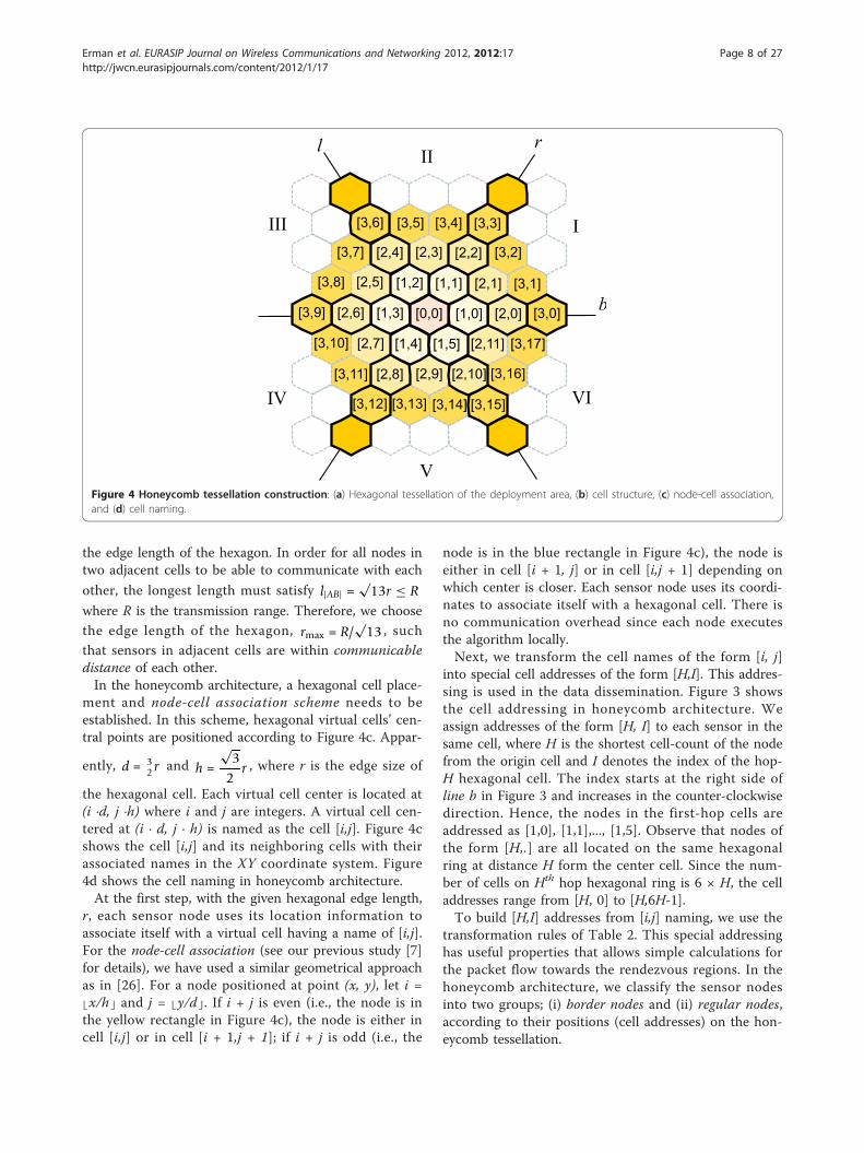
the edge length of the hexagon. In order for all nodes intwo adjacent cells to be able to communicate with each

other, the longest length must satisfy l|AB| =√13r ≤ R

where R is the transmission range. Therefore, we choose

the edge length of the hexagon, rmax = R/√13 , such

that sensors in adjacent cells are within communicabledistance of each other.In the honeycomb architecture, a hexagonal cell place-

ment and node-cell association scheme needs to beestablished. In this scheme, hexagonal virtual cells’ cen-tral points are positioned according to Figure 4c. Appar-

ently, d = 32 r and h =

√32

r , where r is the edge size of

the hexagonal cell. Each virtual cell center is located at(i ·d, j ·h) where i and j are integers. A virtual cell cen-tered at (i · d, j · h) is named as the cell [i,j]. Figure 4cshows the cell [i,j] and its neighboring cells with theirassociated names in the XY coordinate system. Figure4d shows the cell naming in honeycomb architecture.At the first step, with the given hexagonal edge length,

r, each sensor node uses its location information toassociate itself with a virtual cell having a name of [i,j].For the node-cell association (see our previous study [7]for details), we have used a similar geometrical approachas in [26]. For a node positioned at point (x, y), let i =⌊x/h⌋ and j = ⌊y/d⌋. If i + j is even (i.e., the node is inthe yellow rectangle in Figure 4c), the node is either incell [i,j] or in cell [i + 1,j + 1]; if i + j is odd (i.e., the

node is in the blue rectangle in Figure 4c), the node iseither in cell [i + 1, j] or in cell [i,j + 1] depending onwhich center is closer. Each sensor node uses its coordi-nates to associate itself with a hexagonal cell. There isno communication overhead since each node executesthe algorithm locally.Next, we transform the cell names of the form [i, j]

into special cell addresses of the form [H,I]. This addres-sing is used in the data dissemination. Figure 3 showsthe cell addressing in honeycomb architecture. Weassign addresses of the form [H, I] to each sensor in thesame cell, where H is the shortest cell-count of the nodefrom the origin cell and I denotes the index of the hop-H hexagonal cell. The index starts at the right side ofline b in Figure 3 and increases in the counter-clockwisedirection. Hence, the nodes in the first-hop cells areaddressed as [1,0], [1,1],..., [1,5]. Observe that nodes ofthe form [H,.] are all located on the same hexagonalring at distance H form the center cell. Since the num-ber of cells on Hth hop hexagonal ring is 6 × H, the celladdresses range from [H, 0] to [H,6H-1].To build [H,I] addresses from [i,j] naming, we use the

transformation rules of Table 2. This special addressinghas useful properties that allows simple calculations forthe packet flow towards the rendezvous regions. In thehoneycomb architecture, we classify the sensor nodesinto two groups; (i) border nodes and (ii) regular nodes,according to their positions (cell addresses) on the hon-eycomb tessellation.

[1,0]

[1,1][1,2]

[1,3]

[1,4] [1,5]

[2,0]

[2,1] [3,1][2,5][3,8]

[2,2] [3,2][2,4][3,7]

[3,4] [3,3][3,5][3,6]

[2,6]

[2,11] [3,17][2,7][3,10]

[2,10] [3,16][2,8][3,11] [2,9]

[0,0]

[2,3]

[3,14] [3,15][3,13][3,12]

[3,9] [3,0] b

l r

I

II

III

IV

V

VI

Figure 4 Honeycomb tessellation construction: (a) Hexagonal tessellation of the deployment area, (b) cell structure, (c) node-cell association,and (d) cell naming.


Page 8 of 27

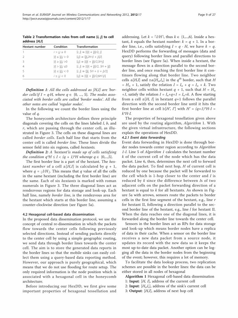
Definition 1: All the cells addressed as [H,I] are ‘bor-der cells’if I = q·H, where q Î {0, ..., 5}. The nodes asso-ciated with border cells are called ‘border nodes’. All theother notes are called ‘regular nodes’.In the following we count the border lines using the

value of q.The honeycomb architecture defines three principle

diagonals covering the cells on the lines labeled l, b, andr, which are passing through the center cell, as illu-strated in Figure 3. The cells on these diagonal lines arecalled border cells. Each half line that starts from thecenter cell is called border line. These lines divide thesensor field into six regions, called hextants.Definition 2: A ‘hextant’is made up of cells satisfying

the condition q*H ≤ I < (q + 1)*H whereqe q Î {0,...,5}.The first border line is a part of the hextant. The hex-

tant number of a cell a[H,I] is calculated by q + 1,where q = ⌊I/H⌋. This means that q value of all the cellsin the same hextant (including the first border line) arethe same. Each of six hextants is marked with romannumerals in Figure 3. The three diagonal lines act asrendezvous regions for data storage and look-up. Eachhalf line, namely border line, is the rendezvous area forthe hextant which starts at this border line, assuming acounter-clockwise direction (see Figure 5a).

4.2 Hexagonal cell-based data disseminationIn the proposed data dissemination protocol, we use theconcept of central re-dissemination in which the packetsflow towards the center cells following previouslyselected directions. Instead of sending packets directlyto the center cell by using a simple geographic routing,we send data through border lines towards the centercell. The aim is to store the generated data reports inthe border lines so that the mobile sinks can easily col-lect them using a query-based data reporting method.However, our approach is purely geographical, whichmeans that we do not use flooding for route setup. Theonly required information is the node position which isassociated with a hexagonal cell in the honeycombarchitecture.Before introducing our HexDD, we first give some

important properties of hexagonal tessellation and

addressing. Let k = ⌈I/H⌉, thus k Î {1,...,6}. Inside a hex-tant, k equals the hextant number: k = q + 1. In a bor-der line, i.e., cells satisfying I = q · H, we have k = q.HexDD performs the forwarding of messages (data andquery) following border lines and parallel directions toborder lines (see Figure 5a). When inside a hextant, themessage flows in a direction parallel to the second bor-der line, and once reaching the first border line it con-tinues flowing along that border line. Two neighborcells a[H,I] and na[Hn,In] in the qth border, such that H= Hn + 1, satisfy the relation I = In + q = In + k. Twoneighbor cells within hextant q + 1, such that H = Hn

+1, satisfy the relation I = In+q+1 = In+k. A flow startingfrom a cell s[H, I] in hextant q+1 follows the paralleldirection with the second border line until it hits thefirst border line at cell b[H’, I’] with H’ = (q+1)*H-I =k*H-I.The properties of hexagonal tessellation given above

are used by the routing algorithm, Algorithm 1. Withthe given virtual infrastructure, the following sectionsexplain the operations of HexDD.4.2.1 Event data forwardingEvent data forwarding in HexDD is done through bor-der nodes towards center region according to Algorithm1-I. Line 5 of Algorithm 1 calculates the hextant numberk of the current cell of the node which has the datapacket. Line 6, then, determines the next cell to forwardthe data packet. To find next hop, H of current cell isreduced by one because the packet will be forwarded tothe cell which is 1-hop closer to the center and I isreduced by k since the difference between Is of twoadjacent cells on the packet forwarding direction of ahextant is equal to k for all hextants. As shown in Fig-ure 5a with arrows, sensors route the packets to bordercells in the first line segment of the hextant, e.g., line rfor hextant II, following a direction parallel to the sec-ond border line of the hextant, e.g., line l for hextant II.When the data reaches one of the diagonal lines, it isforwarded along the border line towards the center cell.Sensors in the border lines act as RPs for data storage

and look-up which means border nodes have a replicaof data in their cache. When a sensor on the border linereceives a new data packet from a source node, itupdates its record with the new data so it keeps themost up-to-date data packet. Another option can be log-ging all the data in the border nodes from the beginningof the event; however, this requires a lot of memory.To facilitate the data lookup process, two replication

schemes are possible in the border lines: the data can beeither stored in all nodes of hexagonalAlgorithm 1 Hexagonal cell-based data dissemination1: Input: [H, I], address of the current cell2: Input: [Hs,Is], address of the sink’s current cell3: Output: [H,I], address of next hop cell

Table 2 Transformation rules from cell name [i, j] to celladdress [H,I]

Hextant number Condition Transformation

1 i > j,j ≥ 0 [i, j] ⇒ [(|i| + |j|)/2, j]

2 |i| ≤ |j|,j > 0 [i,j] ⇒ [|j|,2H-(i + j)|2]

3 |i| ≥ |j|,j >0 [i,j] ⇒ [(|i| + |j|)/2,3H-j]

4 |i| > |j|,j ≤0 [i, j] ⇒ [(|i| + |j|)/2, 3H + |j|]

5 |i| ≤ |j|,j < 0 [i, j] ⇒ [|j|, 5H + (i + j)/2]

6 i ≥ j,j < 0 [i,j] ⇒ [(|i| + |j|)/2,6H-\j\]


Page 9 of 27

4: I. Find next hop cell towards center5: k = ⌈I/H⌉6: [H,I] ⇐ [H-1,I-k]7: II. Find next hop cell towards sink8: ks = ⌈Is/Hs⌉9: H ⇐ H + 110: if H <= ks Hs -Is then11: I ⇐ I+ks-1//In the border line12: else13: I ⇐ I+ks //within the hextant14: end ifcells or just in the cell-leader of each cell. The first

scheme needs a fine-tuning of border line width, w, toprevent an increase of congestion under high traffic loadconditions, while the second one requires a periodiccell-leader election and a replication mechanism. As in[17,30], we disregard the lines’ width w. We assume thateach border line covers only one cell (see Figure 5b).The HexDD keeps the traffic flow in all regions of the

network nearly balanced because honeycomb architec-ture divides the network space into six partitions andeach partition uses a different border line segment fordata dissemination; therefore, the traffic is spreadamong the different border lines.4.2.2 QueryingIn order to retrieve specific data, a sink sends a querytowards the center by using Algorithm 1-I. The data andquery packets are sent towards the center by using thesame forwarding directions which are shown in Figure5a. The first border node which receives the query for-wards it towards the center cell. Each node in the

border cells checks its cache when it receives a query. Ifthe data requested is in the cache of a border node, itsends data back to the sink. Replicating data on the bor-der cells can decrease the cost of data look-up and thedata delivery latency.4.2.3 Event data delivery to sinkTo send data towards the sink, the reverse path of thesink ’s query forwarding path can be calculated byusing the cell address of the sink as given in the Algo-rithm 1-II, or can be stored in the query packet. Theforwarding directions of the data packets from centerto the sinks are exactly the opposite directions of thearrows shown in Figure 5a. Line 8 of the Algorithm 1calculates the hextant number of the sink’s currentcell. Line 9 increases the H by one to get to the nexthexagonal ring which is 1-hop closer to the hexagonalring of the sink’s cell. The data first travels in one ofthe border lines according to hextant number ks ofsink’s cell. In line 10, H is compared with ksHs - Is todetermine the number of hops that the packet shouldbe forwarded along the border line. Thus, the condi-tion in line 10 ensures that the packet does not gofurther on the border line when it reaches the turningpoint towards the sink. If the packet is still on the bor-der line, I is increased by ks -1 in line 11. When thepacket reaches the cell which is on the same line (i.e.,line s parallel to line r in Figure 5b) where sink’s cell isalso located, the packet is forwarded towards the insideof the hextant. Within the hextant, I of the current cellis increased by ks in line 13 until the packet reachesthe cell of the sink.

I

II

III

IV

V

VI

b

l r

[0,0] [1,0] [2,0]

s

[1,3][2,6][3,9]

[2,4]

[3,6]

[1,2]

[4,8][5,11]

[6,14]

[1,4]

[2,8]

[3,12][4,15][5,18]

[3,1]

[4,2]

[5,3]

query

data

data

k=1

k=2

k=3

k=4

k=5

k=6

{kHs- I s= 2 hops[3,10]

[4,14] [3,11]

[2,7]

(a) (b)Figure 5 HexDD in honeycomb tessellation: (a) Packet forwarding directions, (b) data and query dissemination.


Page 10 of 27

Before sending data to a regular node, the algorithmalways checks if there is a sink node in the next hopcell. If so, the data is sent to the sink in the next cell.Otherwise, it sends the data packet to a sensor node inthe next cell until the packet reaches to a sink.Figure 5b shows the data and query dissemination in

HexDD. If there is no neighbor node to forward thepacket (i.e., query or data packet) in the next 2-hop cellscalculated by the Algorithm 1, the protocol switches toroute recovery procedure explained in the followingsection.

4.3 Handling imperfect conditions of wirelesscommunicationIn our hexagonal tessellation construction, we considera widely used assumption for transmission range. Allsensors have the same circular transmission range, R.However, in real sensor deployed environments, radioirregularity (i.e., non-uniform transmission range and/ornon-circular transmission range), which obviously affectsthe network connectivity, can be observed. The effect ofthe radio irregularity on our hexagonal tessellationbased routing is that a sensor node a in cell A may notbe able to communicate with some of the sensor nodesin neighboring cells if the transmission range of node ais smaller that R (i.e., Ra <R) or the transmission rangeis non-circular. In case of small difference between Ra

and R, the possibility of having some links to neighbor-ing cells (i.e., connected neighbors to node a) is higher.However, the difference between Ra and R may be highin some environments. In this case, node a cannot com-municate with some of the neighboring cells or it maybe disconnected from the network. Both cases createsome routing holes in the network.An other issue, which can create routing holes, is

localization errors in real deployments. The hexagonaltessellation and our geographic forwarding protocolrely on each node being able to estimate its own coor-dinates. These estimates are highly likely affected by anon-negligible error, which in turn affects the calcu-lated cell addressing [H, I] used for packet forwarding.We use a kind of polar coordinate system to addressthe cells of the tessellation. This addressing schemeserves as a positioning (coordinate) system that isrougher than the coordinates of the sensor nodes, witha precision appropriate for the transition range. Alocalization estimate with a reasonable error err < r,where r is the edge length of a hexagonal cell, willresult in the same cell address [H, I]. Therefore, thepacket forwarding mechanism will not be affected bythe localization errors. If a given node, which is closeto the boundary of its hexagonal cell, calculates awrong cell address due to localization error, the erro-neous cell address will be one of the neighbor cells of

its real cell. The localization errors may result in someempty cells or some deviations form the regular pathof a packet in HexDD.To handle routing holes and forwarding path devia-

tions created by the imperfect conditions of the wirelessenvironment, in the following section we present a faulttolerance mechanism, which discusses how to determineand bypass the routing holes. This fault tolerancemechanism makes our scheme more feasible in real sen-sor network deployments. As long as a node, which hasa packet to forward, has at least one neighbor in one ofthe neighboring cells, HexDD combined with fault toler-ance mechanism can find an alternative path towardsthe destination of the packet.4.3.1 Fault toleranceAlgorithm 1 assumes that there is at least one nodewhich will perform multi-hop routing within each cell.However, this may not be always the case. Sometimesan area of the network can be lost for different reasons,e.g., environmental reasons such as fire. Holes are cre-ated where there is a group of cells that do not haveany active node inside. Moreover, the imperfect condi-tions of the wireless communication discussed abovemay also create holes in the network. In our previousstudy [8], we discuss possible solutions for fault toler-ance. In this article, we propose and present a completehole detection and bypassing mechanism, which is oneof the most important features that shows how wemaintain the honeycomb architecture even if parts ofthe network are lost.A sensor can easily detect the hole region by checking

its neighbor table, which is updated by periodic beaconpackets. If the sensor has no neighbor on the next 2-hop cells in its radio range, it concludes that there is ahole at that area of the network. Algorithm 2a gives thedetails of HexDD with hole recovery.Algorithm 2 HexDD with Hole Recovery1: Input: [H, I], address of the current cell2: [Hs,Is], address of the sink’s current cell3: N = {n1,..., nm}, list of neighbors4: Na = {[H1,I1],..., [Hm, Im]}, list of cell addresses of

neighbors5: Output: n, next hop neighbor to forward the packet6: I. Find next hop neighbor towards center7: [Hc,Ic] ⇐ Find next hop cell towards center (Alg. 1.I)8: if [Hc, Ic] = [Hi, Ii] Î Na then9: n ⇐ ni {forward data to neighbor in next cell}10: else {there is a hole, enter route recovery}11: n ⇐ nj with Hj the smallest H in Na

12: end if13: II. Find next hop neighbor towards sink14: k = ⌈Is/Hs⌉15: p = Is-(k- 1)Hs

16: if [H, I] in the regular path then


Page 11 of 27

17: [Hc, Ic] ⇐ Find next hop cell towards sink (Alg. 1.II)18: if [Hc, Ic] = [Hi, Ii] Î Na then19: n ⇐ ni {forward data to neighbor in next cell}20: else {there is a hole, enter route recovery}21: n ⇐ nj with [Hj,Ij] where |Hs - Hj| + |Ij - (k - 1)

Hj - p\ is the minimum in Na

22: end if23: else {packet is already in the route recovery}24: n ⇐ nj with [Hj, Ij] where |Hs-Hj| + |Ij -(k- 1)Hj

-p| is the minimum in Na

25: end ifAlgorithm 2-I explains route recovery when sending

packets towards center. Line 7 of the algorithm calcu-lates the next hop cell and line 8 checks if there is aneighbor in the next cell. If there is no neighbor in thenext cell, the algorithm enters route recovery in line 10.To find an alternative path, in line 11, the sensor send-ing its packet (i.e., data or query) towards center checksits neighbors and chooses the neighbor having the smal-lest H, which shows the shortest cell-count of the nodefrom the origin cell (see node C in Figure 6).

Algorithm 2-II explains route recovery when the datais being sent from the center to the sink. In line 15, p,the maximum number of hops between the cell of thesink and the first border line, is calculated. That is thenumber of hops between lines s and b (i.e., first borderline of the hextant) in Figure 6. Line 16 checks if thecurrent node is in the regular path of the packet toknow if the packet is already in the route recovery ornot. The node is in the regular path if H <= Hs - p andI = Hk - (Hs - p) or H > Hs - p and I = (Hs - H)k, other-wise it is off the regular path. If the packet is in the reg-ular path, in line 17, the next hop cell is calculatedbased on Algorithm 1-II. If there is no neighbor in thenext hop cell, the packet enters route recovery at line20. In line 21, the packet is forwarded to the neighbornj within cell [Hj, Ij] where Hj is the closest to Hs and Ijis the closest to p + (k - 1)Hj in neighbor list, Na. Thisapproach achieves to forward the data packet to the cellwhich is on the hexagonal ring that is the closest to thehexagonal ring of the sink. At the same time, it tries tokeep the same distance from the second border line (i.e.,line r) as sink. In Figure 6, where both the sink and the

[0,0] [1,0] [2,0]

s

[1,3][2,6][3,9]

[2,4]

[3,6]

[1,2]

[4,8]

[1,4]

[2,8]

[4,15]

[5,18]

[3,1]

[4,2]

[5,3]

k=1k=2

k=3

k=4

k=5

k=6

{Hs -p

[3,10]

[4,14] [3,11]

[2,7]

[1,1]

[2,2]

[3,3]

[4,4]

[5,5]

p=Is -(k-1)Hs

{[3,2]

2 hops

3 hops

[3,12]

[4,13]

[5,17]

C

[4,11] [3,8]Communication range of node C

[4,12][5,15] [3,0][4,0] [5,0]

[1,5]

[2,10]

[3,15]

[4,20]

[5,25]

[5,13]

[2,1][4,1]

[2,11]

E

[3,16]

[3,17]

[4,22]

[5,1]

[5,2]

[4,3]

xx

Communication range of node E

b

r

Figure 6 Fault tolerance mechanism in HexDD.


Page 12 of 27

node E are located on the line s, node E in cell [2,0] for-wards the packet to the cell [4,1] according to the rulein line 21. If the packet is already in the route recovery,it applies the same rule in line 24.This mechanism is simple and efficient since it avoids

to flood any other control message to inform othernodes about the hole, which is required to find newbridge nodes. This is mainly the advantage of using hon-eycomb tessellation and the chosen addressing scheme.It is important to point out that in HexDD, if a holehappens at the center of the network, the crossing areaof the border lines at the central region should beshifted to a closer location which is not affected by thehole, or the first possible hexagonal ring which excludesthe hole can become the central region.Instead of calculating forwarding path between the

center and a sink by Algorithm 2-II, the reverse pathcan be stored in the query. Since the sink sends a newquery whenever it changes its cell, saving the path inthe query is also efficient. The reverse path in the queryrecovers the hole at the path back to sink (i.e., assumingcommunication links are bidirectional) because whenthe query is being sent towards center, the alternativepath is calculated and stored in the query. However, if anew hole is formed on the path back to the sink, thereverse path stored in the query packet will not be validanymore.

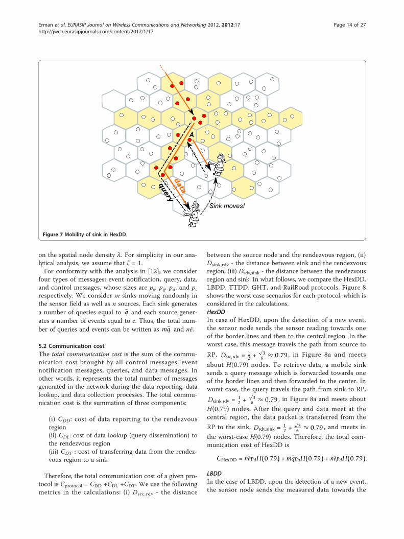
4.4 Mobility supportThe mobility of WSN, where most of the sensors arestationary, can be divided into the source (stimulus)mobility and sink mobility.The impact of source mobility on the dissemination

scheme is very small because when stimulus movesfrom one cell to another cell, a sensor that captures thestimulus becomes the source node and sends the datatowards the center. In our study, the aim is collectingdata about the event. For also tracking the event, eachdata should be augmented with the location of thesource node. On the other hand, to support sink mobi-lity, tracking the location of a sink becomes more criti-cal for data delivery. If the sink moves inside its currentcell, there is no need for another process since the datawill be forwarded to the same neighboring cell until thesink leaves its cell. When the sink moves to anothercell, it needs to send a new query message towards thecenter to inform the center nodes about its new cell. Ifany border node has the requested data in its cache (seenode A in Figure 7), it directly sends data to the newcell of the sink.Although it is assumed that sensor nodes are station-

ary in our study, HexDD can also handle mobility ofsensor nodes. Sensors can easily recalculate their newhexagonal cells by using node-cell association algorithm

[7] while they are moving. However, the uniformdeployment of the sensor network should not beaffected by the mobility of sensors. Thus, HexDD allowsfor a limited mobility of sensor nodes, meaning that thepercentage of moving nodes should be low, so that therisk of having disconnected network partitions and toomany holes in the network will be kept low.

4.5 Resizing rendezvous regionsIn HexDD protocol, most of the traffic is concentratedon the center cell. If the number of events and sinks ishigh, congestion may happen around the center of thenetwork and creates a hot spot region problem. A solu-tion to hot spot region problem is to adjust the size ofthe central region (i.e., number of center cells and num-ber of sensors in the center cells) according to the sizeof the network and the network traffic. The HexDDprotocol can easily establish the size of the centralregion according to the number of sink-source pairs inthe network. While there is only one sink-source pair inthe network, one center cell can be enough to avoidcongestion. On the other hand, for larger number ofsink-source pairs, the central region consisting of centercell and the cells at the first and/or second hexagonalrings can achieve better performance. For this adaptivemechanism, HexDD simply checks the queue size of thenodes in the central region. If the queue size is above acertain threshold, one more hexagonal ring joins thecentral region to serve as rendezvous area. The effect ofcentral region resizing on the performance of HexDDprotocol is evaluated in Section 6.2.5.

5 Performance analysisThis section provides an analytical study of communica-tion cost and hot spot traffic cost of HexDD and otherprotocols given in Section 2. The communication costrepresent the total amount of messages generated in thenetwork during the data dissemination and look up pro-cess. It is important to estimate communication cost sinceit has a direct influence on the network lifetime. The hotspot traffic cost is the total energy consumption of one sin-gle node located at hot regions. It is also importantbecause it restricts the network scalability and lifetime.

5.1 Analysis model and assumptionsWe consider a network with large number of nodesbeing deployed uniformly and distributed over a unitarea. We use the function H(l) as the number of hopson a path between two arbitrary nodes x and y suchthat |x,y| = l is the euclidean distance between thesetwo nodes. According to [31], given a geographical rout-

ing protocol, we have H(l) = ζ 1r where r is the commu-

nication range and ζ ≥ 1 is a scaling factor that depends


Page 13 of 27

on the spatial node density l. For simplicity in our ana-lytical analysis, we assume that ζ = 1.For conformity with the analysis in [12], we consider

four types of messages: event notification, query, data,and control messages, whose sizes are pe, pq, pd, and pcrespectively. We consider m sinks moving randomly inthe sensor field as well as n sources. Each sink generatesa number of queries equal to q and each source gener-ates a number of events equal to ē. Thus, the total num-ber of queries and events can be written as mq and nē.

5.2 Communication costThe total communication cost is the sum of the commu-nication cost brought by all control messages, eventnotification messages, queries, and data messages. Inother words, it represents the total number of messagesgenerated in the network during the data reporting, datalookup, and data collection processes. The total commu-nication cost is the summation of three components:

(i) CDD: cost of data reporting to the rendezvousregion(ii) CDL: cost of data lookup (query dissemination) tothe rendezvous region(iii) CDT : cost of transferring data from the rendez-vous region to a sink

Therefore, the total communication cost of a given pro-tocol is Cprotocol = CDD +CDL +CDT. We use the followingmetrics in the calculations: (i) Dsrc,rdv - the distance

between the source node and the rendezvous region, (ii)Dsink,rdv - the distance between sink and the rendezvousregion, (iii) Drdv,sink - the distance between the rendezvousregion and sink. In what follows, we compare the HexDD,LBDD, TTDD, GHT, and RailRoad protocols. Figure 8shows the worst case scenarios for each protocol, which isconsidered in the calculations.HexDDIn case of HexDD, upon the detection of a new event,the sensor node sends the sensor reading towards oneof the border lines and then to the central region. In theworst case, this message travels the path from source to

RP, Dsrc,rdv = 12 +

√36 ≈ 0.79 , in Figure 8a and meets

about H(0.79) nodes. To retrieve data, a mobile sinksends a query message which is forwarded towards oneof the border lines and then forwarded to the center. Inworst case, the query travels the path from sink to RP,

Dsink,rdv = 12 +

√36 ≈ 0.79 , in Figure 8a and meets about

H(0.79) nodes. After the query and data meet at thecentral region, the data packet is transferred from the

RP to the sink, Drdv,sink = 12 +

√36 ≈ 0.79 , and meets in

the worst-case H(0.79) nodes. Therefore, the total com-munication cost of HexDD is

CHexDD = nepdH(0.79) +mqpqH(0.79) + nepdH(0.79).

LBDDIn the case of LBDD, upon the detection of a new event,the sensor node sends the measured data towards the

query

data

Sink moves!

A

Figure 7 Mobility of sink in HexDD.


Page 14 of 27

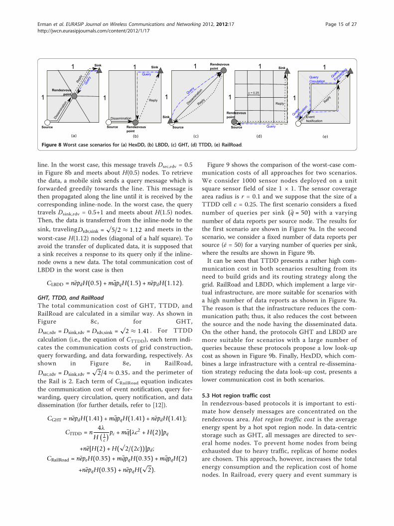
line. In the worst case, this message travels Dsrc,rdv = 0.5in Figure 8b and meets about H(0.5) nodes. To retrievethe data, a mobile sink sends a query message which isforwarded greedily towards the line. This message isthen propagated along the line until it is received by thecorresponding inline-node. In the worst case, the querytravels Dsink,rdv = 0.5+1 and meets about H(1.5) nodes.Then, the data is transferred from the inline-node to thesink, travelingDrdv,sink =

√5/2 ≈ 1.12 and meets in the

worst-case H(1.12) nodes (diagonal of a half square). Toavoid the transfer of duplicated data, it is supposed thata sink receives a response to its query only if the inline-node owns a new data. The total communication cost ofLBDD in the worst case is then

CLBDD = nepdH(0.5) +mqpqH(1.5) + nepdH(1.12).

GHT, TTDD, and RailRoadThe total communication cost of GHT, TTDD, andRailRoad are calculated in a similar way. As shown inFigure 8c, for GHT,

Dsrc,rdv = Dsink,rdv = Drdv,sink =√2 ≈ 1.41 . For TTDD

calculation (i.e., the equation of CTTDD), each term indi-cates the communication costs of grid construction,query forwarding, and data forwarding, respectively. Asshown in Figure 8e, in RailRoad,

Dsrc,rdv = Dsink,rdv =√2/4 ≈ 0.35, and the perimeter of

the Rail is 2. Each term of CRailRoad equation indicatesthe communication cost of event notification, query for-warding, query circulation, query notification, and datadissemination (for further details, refer to [12]).

CGHT = nepdH(1.41) +mqpqH(1.41) + nepdH(1.41);

CTTDD = n4λ

H(1c

)pc +mq[λc2 +H(2)]pq

+ne[H(2) +H(√2/(2c))]pd;

CRailRoad = nepeH(0.35) +mqpqH(0.35) +mqpqH(2)

+nepqH(0.35) + nepqH(√2).

Figure 9 shows the comparison of the worst-case com-munication costs of all approaches for two scenarios.We consider 1000 sensor nodes deployed on a unitsquare sensor field of size 1 × 1. The sensor coveragearea radius is r = 0.1 and we suppose that the size of aTTDD cell c = 0.25. The first scenario considers a fixednumber of queries per sink (q = 50) with a varyingnumber of data reports per source node. The results forthe first scenario are shown in Figure 9a. In the secondscenario, we consider a fixed number of data reports persource (ē = 50) for a varying number of queries per sink,where the results are shown in Figure 9b.It can be seen that TTDD presents a rather high com-

munication cost in both scenarios resulting from itsneed to build grids and its routing strategy along thegrid. RailRoad and LBDD, which implement a large vir-tual infrastructure, are more suitable for scenarios witha high number of data reports as shown in Figure 9a.The reason is that the infrastructure reduces the com-munication path; thus, it also reduces the cost betweenthe source and the node having the disseminated data.On the other hand, the protocols GHT and LBDD aremore suitable for scenarios with a large number ofqueries because these protocols propose a low look-upcost as shown in Figure 9b. Finally, HexDD, which com-bines a large infrastructure with a central re-dissemina-tion strategy reducing the data look-up cost, presents alower communication cost in both scenarios.

5.3 Hot region traffic costIn rendezvous-based protocols it is important to esti-mate how densely messages are concentrated on therendezvous area. Hot region traffic cost is the averageenergy spent by a hot spot region node. In data-centricstorage such as GHT, all messages are directed to sev-eral home nodes. To prevent home nodes from beingexhausted due to heavy traffic, replicas of home nodesare chosen. This approach, however, increases the totalenergy consumption and the replication cost of homenodes. In Railroad, every query and event summary is

1

1

1

1

1

1

1

1

1

1

Source

Sink

Rendezvous point

Dissem

inatio

n

Query

Reply

Source

Rendezvous point

Sink

Query

Reply

c = 0.25

Dissemination

Query

Reply

Sink

Source Rendezvous point

Rendezvous point

Sink

Source

Quer

y

Diss

emina

tion

Reply

EventNotification

QueryCirculation

Reply

(c) (d)(b)(a) (e)

Query

Forward

ing

Query

Notific

ation

Figure 8 Worst case scenarios for (a) HexDD, (b) LBDD, (c) GHT, (d) TTDD, (e) RailRoad.


Page 15 of 27

sent to the Rail, which can be the bottleneck that limitsthe network lifetime. Also, in HexDD queries and datapackets are forwarded toward border lines, which arebecoming hot regions in the network. In this section, weanalyze the hot region traffic cost of GHT, RailRoad,LBDD and our approach HexDD. In the following calcu-lations, T is the amount of energy for a node to transmita single bit, and R is the energy needed to receive a bit.In data-centric storage, the home nodes can be hot

spots, and the hot spot traffic cost can be written as fol-lows [30]:

EHGHT = R[nespd +

1γ

mqspq

]+ T

[1γ

nespd

]

where g is the number of nodes in a replica set includ-ing the home node. It means a home node has g - 1replicas. When g is set to 1, there exists no replicanodes but the home nodes. There are s different eventtypes in the network. We assume that there is only oneevent type (s = 1) in the network for the calculations.All data and query packets coming from sources andsinks are received by the home node, i.e.,

R(nepd + 1

γmqpq

). The home node, then, transmits the

data packet to the sinks, i.e., T(1γnepd

).

The hot spot traffic cost of Railroad can be written asfollows [30]:

EHRR =1NR

[RnepeNST + RmqpqNRT+

Tnepe + Tnepq + TmqpqNRT

]

where NR, NST, and NRT stand for the number of therail nodes, the number of rail nodes in a stationb, andthe number of nodes that a query stays in a single touraround Rail, respectively. In an event notification pro-cess, one node out of NST nodes transmits the eventnotification packet (i.e., Tnēpe) sent by a source node

and NST nodes receive this event notification packet (i.e., RnēpeNST). For query flooding in the Rail, NRT nodesout of NR nodes receive a query packet (i.e., RmqpqNRT )sent by a sink and NRT nodes out of NR nodes transmitthe query packet (i.e., TmqpqNRT ). Finally, one node outof NRT nodes transmits the query packet to the sourcenode (i.e., Tnēpq). The data is directly sent from sourceto sink with GF.The hot spot traffic cost of LBDD can be written as

follows:

EHLBDD =1NL

[RnepdNST + RmqpqNL+

Tnepd + TmqpqNL

]

where NL is number of inline nodes and NST is thenumber of inline nodes in a station which is a smallgroup of nodes in the virtual line. In the data dissemina-tion process, NST nodes out of NL nodes receive a datapacket (i.e., RnēpdNST) sent by a source node. For queryflooding in the line/strip, NL nodes receive the querypacket (i.e., RmqpqNL ) sent by a sink and NL nodes

transmit the query packet (i.e., TmqpqNL ). Finally, onenode out of NST nodes sends the data packet to the sink(i.e., Tnēpd). GF is used to send data to the sink.The hot spot traffic cost of HexDD is as follows,

EHHexDD =1

3NBL

[2Rnepd

NBL2NC

+ RmqpqNBL2NC

+

2Tnepd NBL2NC

+ Tmqpq NBL2NC

]

where NBL is the number of border nodes in a diago-nal line, and NC is the average number of nodes in acell. NBL/2NC is the number of cells on a border linec.Since one node per cell transmit or receive the packets,NBL/2NC is also the number of nodes having the packetson a border line. In data dissemination and data transferprocess, a node in each cell receives and transmits thedata packet along the diagonal line (i.e.,

0

50000

100000

150000

200000

250000

0 50 100 150 200 250

Worst case communication cost

Number of data reports per source

HexDDLBDDTTDDGHT

RailRoad

0

20000

40000

60000

80000

100000

120000

140000

160000

180000

200000

0 50 100 150 200 250

Worst case communication cost

Number of queries per sink

HexDDLBDDTTDDGHT

RailRoad

(a) (b)

Figure 9 Worst case communication costs (m = 5 sinks, n = 10 sources): (a) number of queries q = 50 , (b) number of events ē = 50.


Page 16 of 27

q = 50 ). The sink’s query travels the border line (i.e.,

Rmqpq NBL2NC

+ Tmqpq NBL2NC

). The above formula for the hot

spot traffic cost of HexDD can be written as:

EHHexDD =1

3NC

[Rnepd + Rmqpq(0.5)+

Tnepd + Tmqpq(0.5)

]

For calculation of the hot spot traffic costs of the pro-tocols, the number of sources n and number of sinks mvary between 1 to 18 in the first set of analysis to seethe effect of number of sinks and sources on the hotspot regions. In the second set of analysis, we set n to 5and m to 15 and the number of queries per sink andthe number of events per source are varied to see theeffect of the network traffic generated by sinks andsources on the hot spot regions. Total number of nodesN in a sensor field of 1000 m × 1000 m is set to 10000.The number of rail nodes NR is 8% of total nodes andthe number of nodes that receive a query in the RailNRT is 480. In the analysis, we use the same values usedin [30] for the number of rail nodes in a station NST,and R/T which are taken as 16 and 3/8, respectively.Both the width of the Rail and the station are set to 40m, that is the radio range of the sensor nodes. Based onthe values given above, the average number of nodes ina cell, NC, is 3 in HexDD. We set pe = pc = pq and pd =2 × pq.In Figures 10, 11, and 12 we show the hotspot traffic

cost of HexDD compared with other protocols. In thefirst graphs of Figures 10a, 11a, and 12a, x axis is thenumber of sinks (m) and y axis is the number of sources(n). In the second graphs of Figures 10b, 11b, and 12b, xaxis is the total number of queries (mq) and y axis isthe total number of events (nē). The z axis of the graphsshows the ratio between the hot spot traffic cost ofHexDD (EHHexDD) and the hot spot traffic cost ofanother protocol (EHprotocol). A border node in HexDDprocesses less data than a rendezvous node in the otherprotocol if the ratio EHHexDD/EHprotocol < 1.0. In thefirst set of graphs, the aim is to see the effect of varyingnumber of sinks and sources on the hot spot trafficcosts of the protocols. The second set of graphs showsthe hot spot traffic costs in the event-driven scenario,where the number of event messages per source (ē) islarger than the number of queries per sink (q), and inthe query-based scenario, where the number of queriesper sink is larger than the number of event messagesper source.Figure 10a shows the hot region traffic cost of HexDD

compared with the data-centric storage GHT with vary-ing number of sinks and sources. The result shows thata home node in a data-centric storage has to processmuch more requests than a border node in HexDD

protocol since EHHexDD/EHGHT < 1.0 for all the givenvalues of number of sinks and number of sources. Thisis more remarkable as the number of sources increasesand the number of sinks decreases. In Figure 10b, wherewe vary the number of queries per sink and the numberof data reports per source, the same behavior isobserved as the total number of events increases andthe total number of queries decreases. Both graphs showthat the hot spot traffic cost of HexDD is much lessthan that of a data-centric storage.In Figure 11 we compare the hot region traffic costs of

HexDD and RailRoad. The results in Figure 11a showthat when we have many event sources but a couple ofsinks in the network (i.e., see n = 15, m = 3, andEHHexDD/EHRR = 1.8 in the figure), a border node inHexDD processes much more requests than a rail nodein RailRoad. This is due to the fact that RailRoad doesnot process/forward data reports in the Rail region; onthe other hand, in HexDD diagonal lines are also usedfor data forwarding to cache data on the border nodesfor sink queries. This is an expected results becauseHexDD is designed for networks where the differencebetween the number of sinks and sources is not veryhigh. For instance, when n = 15 and m = 6, the ratioEHHexDD/EHRR = 0.98 so HexDD is still better than Rail-Road. As observed in the figure, when the number ofsinks is greater than or equal to the number of sources,the hot spot traffic cost of HexDD is much less thanthat of RailRoad. Figure 11b presents the results of ascenario having 15 sinks and 5 sources in the network.Apparently, HexDD becomes advantageous over Rail-Road in terms of hot spot traffic cost in the query-drivenscenarios, where the query generation rate is higher thanthe event generation rate. Also, when the total numberof queries is close to the total number of events,HexDD still processes less requests on the rendezvouslines than RailRoad.Figure 12 compares the hot region traffic costs of

HexDD and LBDD. It has a similar behavior with theprevious graphs for RailRoad comparison because theratio EHRR/EHLBDD ≃ 0.6 for the given network specifi-cations. This means that an inline node of LBDDalready processes more requests in the line-based ren-dezvous region than a rail node in RailRoad. Also, asshown in Figure 12a,b, an inline node of LBDD pro-cesses much more requests than a border node ofHexDD in most of the cases. The same observationspreviously discussed for RailRoad comparison are alsovalid for LBDD comparison. Only the ratio EHHexDD/EHLBDD is smaller than the ratio EHHexDD/EHRR for thesame inputs. For instance, when n = 15 and m = 6, theratio EHHexDD/EHLBDD = 0.59.In this section, we analyzed the influence of the ren-

dezvous region placement on the number of packets (i.


Page 17 of 27

e., query and data) processed (i.e., received/transmitted)in each protocol during the data dissemination. We alsoanalyzed the effect of network traffic generated by sinksand sources on the load created in rendezvous regions

of different protocols. In these analytical analyses, net-working issues, such as packet drops, retransmissions,congestion near hot spot regions, were not taken intoaccount. In the following section, we evaluate the

0

3

6

9

12

15

18 0

3

6

9

12

15

18

0.11

0.12

0.13

0.14

0.15

0.16

0.17

0.18

m (number of sinks) n (number of sources)

EHHexDD/EHGHT

e = 50 q = 50

Total number of queries (mq) Total number of events (ne)

EHHexDD/EHGHT

15 5N = 10, 000

pd= 2pq

050

100150

200250

300

0

50

100

150

200

0.10

0.12

0.14

0.16

0.18

0.20

(a) (b)Figure 10 Analysis of hot spot traffic cost of HexDD compared with GHT: (a) number of sinks vs. number of sources, (b) total number ofqueries vs. total number of events.

0

36

912

15

180

3

6

9

12

15

180.0

0.2

0.4

0.6

0.8

1.0

1.2

1.4

1.6

1.8

2.0


EHHexDD/EHRR

e = 50 q = 50

Total number of queries (mq) Total number of events (ne)

EHHexDD/EHRR

15 5N = 10, 000

NR = 800NRT = 480NST =16pd= 2pq

0

50100

150200

250

3000

50

100

150

2000.0

0.2

0.4

0.6

0.8

1.0

1.2

(a) (b)

Figure 11 Analysis of hot spot traffic cost of HexDD compared with RailRoad: (a) number of sinks vs. number of sources, (b) total numberof queries vs. total number of events.


Page 18 of 27

performance of the protocols by simulating realistic sce-narios and networking conditions.

6 Performance evaluationFor the purpose of performance evaluation, we comparethe proposed protocol, HexDD, with two other rendez-vous-based approaches, LBDD, and TTDD. We chooseTTDD and LBDD for the comparison since we wouldlike to investigate the effect of using hexagonal tessella-tion instead of rectangular grids and using three diago-nal lines acting as rendezvous area instead of only oneline-based region. The simulations were carried out toevaluate routing performance and the fault-toleranceperformance of the protocols. We also investigate theeffect of central region size on HexDD protocol.For this purpose, first, we analyze the protocols with

varying number of sink-source pairs. Second, we explorethe impact of sink mobility (i.e., sink’s maximum speed)on the performance of these protocols. We then analyzethe fault-tolerance performance and vary the total num-ber of holes and the size of holes in the network. Wealso analyze the protocols’ energy distribution mapswhich are important to see hot spot regions created byeach protocol in the network. Indeed, since all datareports and queries are concentrated over the centralregion in HexDD protocol, the hot spot problem canarise, limiting the network lifetime and the scalability.To prevent the central cell from being a bottleneck, it ispossible to design a larger central region, including the

first hexagonal ring, to better distribute the load amongits nodes. Therefore, we, finally, test the routing perfor-mance of HexDD with different size of central region (i.e., center with one cell or center with first hexagonalring) to see if we can reduce energy consumption pernode at the center with a larger central rendezvousregion.

6.1 Simulation environmentHexDD protocol is implemented and tested in NS2 [32].To guarantee a fair comparison between TTDD andHexDD, we set simulation parameters comparable tothose used in [15]. This includes simulation of IEEE802.11 DCF as the underlying MAC and an energymodel in which a sensor’s transmitting, receiving andidling power consumptions are set to 0.66W, 0.395W,and 0.035W, respectively. Although IEEE 802.15.4 is astandard developed to meet the needs for low-powerand low-cost wireless communication, we prefer to useIEEE 802.11 standard in our simulations to be compar-able with previous studies. A comparative performancestudy of IEEE 802.15.4 and IEEE 802.11 can be found in[33]. The cell size in TTDD is set to 600 m. In LBDD,width of the virtual line is set to 250 m. Each node hasa transmission range of 250 m. For routing performancesimulations, 250 sensor nodes are randomly distributedon a 2000×2000 m2 field. For fault-tolerance perfor-mance simulations, 210 nodes are randomly distributedon a 1500×1500 m2 field. Each simulation run lasts for

0

36

912

15

180

3

6

9

12

15

180.0

0.2

0.4

0.6

0.8

1.0

1.2


EHHexDD/EHLBDD

e = 50 q = 50

Total number of queries (mq)Total number of events (ne)

EHHexDD/EHLBDD

15 5N = 10, 000

NL = 400NST =16pd= 2pq

0

50100

150200

250

3000

50

100

150

2000.0

0.2

0.4

0.6

0.8

1.0

(a) (b)

Figure 12 Analysis of hot spot traffic cost of HexDD compared with LBDD: (a) number of sinks vs. number of sources, (b) total number ofqueries vs. total number of events.


Page 19 of 27

200 s. Results are averaged over six random networktopologies. A source generates one data packet per sec-ond, so there are in total 200 data packets/source sent.Sinks’ mobility follows the standard linear mobilitymodel. Mobile sinks could attain a maximum speed upto 14 m/s with 5 s pause time. The stimuli remain staticduring the simulation time. For different sets of simula-tions, speed, and pause times of sink are varied.We use the following metrics to evaluate the perfor-

mance of the protocols: (i) Data delivery ratio: definedas the ratio between the total number of data packetsreceived by the sinks and the total number of event datagenerated by the sources; (ii) Data delivery delay:defined as the total time elapsed between the data gen-eration by a source and its reception by a sink, alsoaveraged over all sink-source pairs; and (iii) Energy con-sumption: defined as the communication (transmittingand receiving) energy the network consumes; the idleenergy is not counted since it depends largely on thedata generation interval and does not indicate the effi-ciency of data delivery.

6.2 Simulation resultsFor each metric, we have evaluated the performance infour different scenarios:

• Impact of the number of sink-source pairs: In thisscenario, the number of sink-source pairs is varied.Mobile sinks could attain a maximum speed up to10 m/s with 5 s pause time.• Impact of sink mobility: We test the performanceof the protocols under both low mobility (i.e., 4-5km/h for walking humans) and high mobility (e.g.,50-60 km/h for UAVs) scenarios. The sinks’ speedsare set to 0, 5, 10, 15, and 20 m/s (0 to 72 km/h)with a pause time of 5 s, where the speed of 0 m/sallows for static sinks in the network. The speed 20m/s means that a sink crosses the border of a cellapproximately every 7 s (i.e., 2r = 138.5 m which isthe longest distance in a hexagon, 138.5/20 ≅ 7 s) inHexDD. There are 6 sink-source pairs in thisscenario.• Impact of the number of holes in the network: Tosee the performance of the fault tolerance mechan-ism, we create holes in the network for this scenar-ios. Each different shaped and middle sized holecovering 5 cells in the network is randomly gener-ated and positioned on a hextant or over the borderlines. The number of sources is equal to the numberof holes in the network. Each source is placed on alocation where it is affected by at least one hole.Three destination sinks are chosen randomly in thenetwork.

• Impact of the size of holes in the network: In thisscenario, we test the performance of the fault toler-ance mechanism in terms of size of holes. In this setof simulations, there are one sink-source pair andone hole in the network. The size and the shape ofthe hole is changed for different runs. The size ofthe hole is represented as the number of cells thatthe hole covers.

6.2.1 Data delivery ratioIn the first three scenarios showing impact of sink-source pairs, sink mobility, and number of holes, weobserve that HexDD outperforms others, as shown inFigure 13a-c. In these scenarios data delivery ratio forLBDD and TTDD is in the range 86%-98%, whereas forHexDD the range is 94%-100%. The use of six borderlines in HexDD allows to better distribute the loadamong the nodes inside the rendezvous area. Thisassures high delivery ratio even for large number ofsink-source pairs (see Figure 13a). Even though there isno explicit mobility tracking scheme in HexDD, it func-tions well under high mobility (see Figure 13b). Thehole recovery mechanism in HexDD achieves a morereliable packet delivery than LBDD and TTDD (see Fig-ure 13c).Figure 13d shows the data delivery ratio vs. increasing

hole size. The hole recovery mechanism in HexDDworks well also for varying size of holes, as a result thedata delivery ratio is high. TTDD performs better insuch a scenario. Its grid structure allows the data pack-ets to find other paths to bypass a hole even when wehave a large hole in the network, thus the success ratioof TTDD is the highest. LBDD has the lowest perfor-mance because for larger holes the GF has more diffi-culties to find a path along the boundary of the holeand most of the time fails to route packets across thebig holes.6.2.2 Data delivery delayAs shown in Figure 14a-d, in all scenarios TTDD hasthe highest delay. In Figure 14a, the increase in thedelay of TTDD is due to the time spent for the creationand the propagation of the grid for each source. Thereason of the high delay of TTDD in Figure 14b is thatsink mobility causes the reconstruction of a new pathbetween the sink and the dissemination point on thegrid every time the sink changes its local cell. TTDDhas the highest delay in Figure 14c,d since the alterna-tive paths along the grids to bypass holes are in most ofthe cases longer than the possible shortest path betweena source and a sink. The delay of LBDD and HexDD areclose to each other in all scenarios. The delay of HexDDis smaller than LBDD in scenarios showing the impactsof sink-source pairs, and sink mobility in Figure 14a,b,respectively. This is because a sink can access data


Page 20 of 27

stored in the border lines in a short time in HexDDeven while it is moving around the network. In routinghole scenarios, the delay of LBDD is lower that HexDDas shown in Figure 14c,d. The reason of this is that inLBDD more packets get stuck in the holes and the lostpackets are not included in the delay results. HexDDtries to forward packets along the boundary of a holevia the shortest possible path so it also has a low delay.6.2.3 Energy consumptionIn all scenarios shown in Figure 15, TTDD presents arather higher energy consumption than HexDD andLBDD. In varying sink-source pairs and sink mobilityscenarios (see Figure 15a,b, respectively), the energyconsumption of TTDD is the highest since there is noglobal virtual infrastructure in TTDD, instead for eachsource node a separate grid structure is constructed. Inrouting hole scenarios (see Figure 15c,d), the energyconsumption of TTDD is the highest due to long dataforwarding paths on the grid between sources and sinksto evade holes. Thus, in TTDD there is a trade-offbetween the energy spent for recovering holes and the

data delivery ratio. TTDD achieves a high data deliveryratio in hole recovery scenarios (see Figure 13d), but itis very costly.Energy consumption of HexDD is the lowest in all

scenarios as shown in Figure 15. The global virtual hex-agonal infrastructure of HexDD results in lower energyconsumptions since data packets are required to sendonly towards the rendezvous nodes (i.e., nodes in borderlines). In routing hole scenario shown in Figure 15c, theenergy consumption of HexDD first increases until acertain point (see between 0 and 3 holes in the figure)since it achieves to recover holes and find paths betweensources and sinks. After that point, the energy consump-tion decreases slightly because the data delivery ratio ofHexDD also decreases slightly (see Figure 13c). Lessdata forwarding results in less energy consumption.Energy consumption of HexDD in Figure 15d has also asimilar behavior. The energy consumption of LBDD ishigher than HexDD, but it stays more or less samewhen we increase the number or size of holes in thenetwork (see also Figure 13c,d, respectively). This is

(a) (b)

(c) (d)

0.7

0.75

0.8

0.85

0.9

0.95

1

0 5 10 15 20

Data Delivery Ratio (%)

Maximum Sink Speed (m/s)

HEXDDLBDDTTDD

0.6

0.65

0.7

0.75

0.8

0.85

0.9

0.95

1

0 1 2 3 4 5 6


Number of Holes

HEXDDLBDDTTDD 0.6

0.65

0.7

0.75

0.8

0.85

0.9

0.95

1

1 2 3 4 5 6 7 8 9 10


Size of Hole (Number of Cells)

HEXDDLBDDTTDD

0.7

0.75

0.8

0.85

0.9

0.95

1

0 2 4 6 8 10


Number of Sinks and Sources

HEXDDLBDDTTDD

Figure 13 Data delivery ratio of the protocols against varying (a) number of sink-source pairs, (b) sink speed, (c) number of holes,and (d) size of holes.


Page 21 of 27

because the LBDD protocol always tries to find a pathon the border of a hole and it forwards data packetuntil it gets stuck at some point. Therefore, LBDD stillconsumes energy on the same level although it has alower data delivery ratio (see Figure 13c,d) when weincrease the number or size of holes in the network.6.2.4 Hotspot regionsThe use of a virtual infrastructure for the data dissemi-nation can lead to the hot spot problem. Indeed, as alldata reports and queries are concentrated over the ren-dezvous area, the hot spot problem can arise, limitingthus the network lifetime and the scalability. In this setof simulations, we analyze hot spot region in a networkhaving six sources and one sink, which is located at dif-ferent locations for three different scenarios. The simu-lation run lasts for 600 s.Figure 16 shows the distribution map of energy con-

sumption for the protocols. Energy consumptions inhello packet transmissions for neighbor discovery andidle mode are not shown in the maps since it dependslargely on the data generation interval and does notindicate the efficiency of the protocol. Although energy

consumption is highly variable and depends on the cur-rent location of the sink and source, an importantobservation about our approach is that nodes in theborder lines experience a higher energy consumption,which shows that energy consumption is distributedamong the nodes in the rendezvous region. On theother hand, the nodes close to the center of the networkconsume the highest energy, as expected. The maximumenergy expenditure of a center node is around 1200W(see Table 3). It is, therefore, observed that in HexDDthe network lifetime is defined by a few nodes that areat the center of the network (see Figure 16c). Concern-ing LBDD, we notice that energy consumption is alsodistributed among the nodes in the rendezvous region,which is the central strip in the network. However,LBDD also has the highest energy consumption (around900W) at the center of the network (see Figure 16b).The sensor node, which consumes the highest energy inthe network, spends around 1000W in TTDD. Since aseparate grid structure is constructed by each individualsource in TTDD, the energy consumption is equallyhigh throughout the network (see Figure 16a). This

0

20

40

60

80

100

120

0 2 4 6 8 10

Data Delivery Delay (msec)


HEXDDLBDDTTDD

0

20

40

60

80

100

120

0 5 10 15 20



HEXDDLBDDTTDD

10

15

20

25

30

35

40

0 1 2 3 4 5 6


Number of Holes

HEXDDLBDDTTDD

10

15

20

25

30

35

1 2 3 4 5 6 7 8 9 10



HEXDDLBDDTTDD

(a) (b)

(c) (d)Figure 14 Data delivery delay of the protocols against varying (a) number of sink-source pairs, (b) sink speed, (c) number of holes,and (d) size of holes.


Page 22 of 27

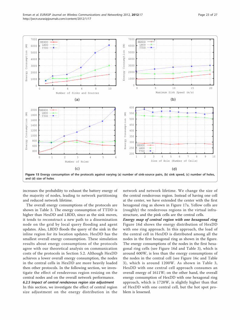
increases the probability to exhaust the battery energy ofthe majority of nodes, leading to network partitioningand reduced network lifetime.The overall energy consumptions of the protocols are

shown in Table 3. The energy consumption of TTDD ishigher than HexDD and LBDD, since as the sink moves,it tends to reconstruct a new path to a disseminationnode on the grid by local query flooding and agentupdates. Also, LBDD floods the query of the sink in theinline region for its location updates. HexDD has thesmallest overall energy consumption. These simulationresults about energy consumptions of the protocolsagree with our theoretical analysis on communicationcosts of the protocols in Section 5.2. Although HexDDachieves a lower overall energy consumption, the nodesin the central cells in HexDD are more heavily loadedthen other protocols. In the following section, we inves-tigate the effect of rendezvous region resizing on thecentral nodes and on the overall network performance.6.2.5 Impact of central rendezvous region size adjustmentIn this section, we investigate the effect of central regionsize adjustment on the energy distribution in the

network and network lifetime. We change the size ofthe central rendezvous region. Instead of having one cellat the center, we have extended the center with the firsthexagonal ring as shown in Figure 17a. Yellow cells are(roughly) the rendezvous regions in the virtual infra-structure, and the pink cells are the central cells.Energy map of central region with one hexagonal ringFigure 16d shows the energy distribution of HexDDwith one ring approach. In this approach, the load ofthe central cell in HexDD is distributed among all thenodes in the first hexagonal ring as shown in the figure.The energy consumptions of the nodes in the first hexa-gonal ring cells (see Figure 16d and Table 3), which isaround 600W, is less than the energy consumptions ofthe nodes in the central cell (see Figure 16c and Table3), which is around 1200W. As shown in Table 3,HexDD with one central cell approach consumes anoverall energy of 1611W; on the other hand, the overallenergy consumption of HexDD with one hexagonal ringapproach, which is 1728W, is slightly higher than thatof HexDD with one central cell, but the hot spot pro-blem is lessened.

(a) (b)

(c) (d)

0

1000

2000

3000

4000

5000

6000

7000

0 2 4 6 8 10

Energy Consumption (W)


HEXDDLBDDTTDD

0

1000

2000

3000

4000

5000

6000

7000

0 5 10 15 20



HEXDDLBDDTTDD

400

600

800

1000

1200

1400

1600

1800

2000

0 1 2 3 4 5 6


Number of Holes

HEXDDLBDDTTDD

200

250

300

350

400

450

500

550

600

1 2 3 4 5 6 7 8 9 10



HEXDDLBDDTTDD

Figure 15 Energy consumption of the protocols against varying (a) number of sink-source pairs, (b) sink speed, (c) number of holes,and (d) size of holes.


Page 23 of 27

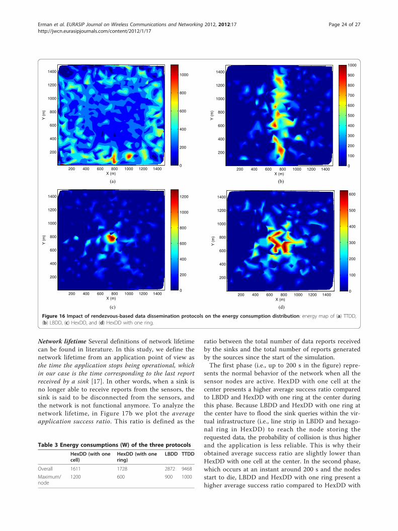
Network lifetime Several definitions of network lifetimecan be found in literature. In this study, we define thenetwork lifetime from an application point of view asthe time the application stops being operational, whichin our case is the time corresponding to the last reportreceived by a sink [17]. In other words, when a sink isno longer able to receive reports from the sensors, thesink is said to be disconnected from the sensors, andthe network is not functional anymore. To analyze thenetwork lifetime, in Figure 17b we plot the averageapplication success ratio. This ratio is defined as the

ratio between the total number of data reports receivedby the sinks and the total number of reports generatedby the sources since the start of the simulation.The first phase (i.e., up to 200 s in the figure) repre-

sents the normal behavior of the network when all thesensor nodes are active. HexDD with one cell at thecenter presents a higher average success ratio comparedto LBDD and HexDD with one ring at the center duringthis phase. Because LBDD and HexDD with one ring atthe center have to flood the sink queries within the vir-tual infrastructure (i.e., line strip in LBDD and hexago-nal ring in HexDD) to reach the node storing therequested data, the probability of collision is thus higherand the application is less reliable. This is why theirobtained average success ratio are slightly lower thanHexDD with one cell at the center. In the second phase,which occurs at an instant around 200 s and the nodesstart to die, LBDD and HexDD with one ring present ahigher average success ratio compared to HexDD with

X (m)

Y (m

)

200 400 600 800 1000 1200 1400

200

400

600

800

1000

1200

1400

0

200

400

600

800

1000

X (m)

Y (m

)

200 400 600 800 1000 1200 1400

200

400

600

800

1000

1200

1400

0

100

200

300

400

500

600

700

800

900

1000

X (m)

Y (m

)

200 400 600 800 1000 1200 1400

200

400

600

800

1000

1200

1400

0

200

400

600

800

1000

1200

0

100

200

300

400

500

600

(a) (b)

(c) (d)

200 400 600 800 1000 1200 1400

200

400

600

800

1000

1200

1400

X (m)

Y (m

)

Figure 16 Impact of rendezvous-based data dissemination protocols on the energy consumption distribution: energy map of (a) TTDD,(b) LBDD, (c) HexDD, and (d) HexDD with one ring.

Table 3 Energy consumptions (W) of the three protocols

HexDD (with onecell)

HexDD (with onering)

LBDD TTDD

Overall 1611 1728 2872 9468

Maximum/node

1200 600 900 1000


Page 24 of 27

one cell. Since they have a larger virtual infrastructure,the energy consumption of LBDD and HexDD with onering is distributed over the entire rendezvous area,avoiding thus the hot spot problem and the existence of

critical nodes such as the central nodes of HexDD withone cell at the center. Larger infrastructure introducesmore redundancy between nodes, increasing the proto-col robustness. This directly impacts the application

HexDD with one cell HexDD with one ring

(a)

0

0.2

0.4

0.6

0.8

1

0 200 400 600 800 1000Average Application Success Ratio

Time (sec)

HEXDD-one ringHEXDD-one cell

LBDD

(b)Figure 17 Average application success ratio: (a) central rendezvous region size adjustment, (b) average application success ratio.


Page 25 of 27

success ratio which remains higher with LBDD andHexDD with one ring than with HexDD with one cen-tral cell.Another way for better distributing the load or the

energy consumption over the network in HexDD protocolis shifting the central cells to another location in the net-work (for both one-cell and one-ring approaches) androtating the border lines over time. The central cell shiftingcan be easily done by taking the new position of the centeras the reference point in the node-cell association process.For rotating border lines over the center cell, the wholehoneycomb tessellation should be rotated to keep the sameaddressing scheme for routing. This requires some addi-tional steps in the node-cell association algorithm.

7 Conclusions and future workIn this article, our goal was designing a routing protocolthat supports mobility of sink and source by keeping thedata delivery ratio as high as possible and data deliverydelay as low as possible, while taking care of energy con-sumption by keeping it low. We proposed a virtual infra-structure called honeycomb architecture and an efficientprotocol for geographical routing of event messages,HexDD, based on this infrastructure. The HexDD usesthe concept of rendezvous region for events and queries.The border lines used as rendezvous areas, which lie onthree main direction of the network, make it faster forsinks to access data. Honeycomb tessellation offersadvantages in terms of algorithmic simplicity in routingand fault tolerance against node failures. HexDD makesthe system resistant to node failures in the virtual infra-structure and helps in quick routing hole recovery in thenetwork. We evaluated analytically the communicationcost and hot region traffic cost of HexDD and saw thatHexDD is a very suitable protocol for applications, wherewe have many mobile sinks and a reasonable number ofsources in the network, such as emergency situation sce-narios. Also, the simulation results show that our archi-tecture helps to minimize overall energy consumptionand keeps the data delivery ratio high even when routingholes exist in the network. To avoid the hot region pro-blem, which may be observed in the border lines and thecentral cells, one solution is to adjust the size of the bor-der lines and shape of the central region according to thesize of the network and the network traffic. In the simu-lations, we show the energy distribution over the networkwhen we have different central regions (i.e., one centralcell or one central ring). As recent studies have beenexploiting heterogeneity in the WSNs, deployment ofhigher energy and communication capacity nodes can beused at the center of the network to leverage the overallsystem capability of HexDD. Deploying more nodes tothese regions is also another solution for the hot spotproblem.

In the future, we plan to investigate the in-networkdata aggregation. Since the forwarding paths along thediagonals of sensor field are shared among all source-sink pairs, it provides an opportunity for similar data tomeet at some common border nodes. Data from multi-ple sources can be aggregated and replaced by a singledata packet and forwarded towards the destined sink.Our proposed scheme can achieve further performancegain by in-network data aggregation. Another issue tobe considered is the effect of underlying MAC protocolon the performance of the data dissemination. It shouldbe further investigated what impacts different MAC pro-tocols have on the system. Designing a MAC protocolwhich can cooperate with networking layer can reducethe impact of MAC on the data dissemination. Sinceour protocol is location-based, the impact of localizationerrors on the performance of the protocol should alsobe further investigated with additional scenariosalthough the fault tolerance mechanism handles posi-tioning errors. The final plan is to implement HexDD inreal nodes and see the effectiveness of the protocol inthe real world scenarios.

EndnotesaFor simplicity in Algorithm 2 we show neighbor check-ing for only next 1-hop cell.bIn RailRoad and LBDD, therendezvous region is divided into smaller subregionscalled station. All the nodes in a station are informedabout the data but one of them forwards data towardssink.c Border line is the half of a diagonal line.

AcknowledgementsThis study had been partially supported by the RECONSURVE project fundedby ITEA2 and Agentschap NL.

Competing interestsThe authors declare that they have no competing interests.

Received: 5 April 2011 Accepted: 16 January 2012Published: 16 January 2012

References1. M Marin-Perianu, C Lombriser, O Amft, P Havinga, G Troster, Distributed

activity recognition with fuzzy-enabled wireless sensor networks, inProceedings of 4th IEEE International Conference on Distributed Computing inSensor Systems, DCOSS ‘08, Santorini Springer Verlag, Greece, pp. 296–313(2008)

2. I Krontiris, Z Benenson, T Giannetsos, F Freiling, T Dimitriou, cooperativeintrusion detection in wireless sensor networks. Wirel Sensor Netw LectureNotes in Computer Science. 5432, 263–278 (2009). doi:10.1007/978-3-642-00224-3_17

3. S Kim, S Pakzad, D Culler, J Demmel, G Fenves, S Glaser, M Turon, Wirelesssensor networks for structural health monitoring, in Proceedings of the 4thinternational conference on Embedded networked sensor systems, SenSys ‘06,Boulder, Colorado, USA, pp. 427–428 (2006)

4. A Erman-Tuysuz, L van Hoesel, P Havinga, J Wu, Enabling mobility inheterogeneous wireless sensor networks cooperating with UAVs formission-critical management. IEEE Wirel Commun. 15(6), 38–46 (2008)

5. C Intanagonwiwat, R Govindan, D Estrin, Directed diffusion: a scalable androbust communication paradigm for sensor networks, in Proceedings of the


Page 26 of 27

6th annual international conference on Mobile computing and networking,MobiCom’00, Boston, MA, USA, pp. 56–67 (2000)

6. E Hamida, G Chelius, Strategies for data dissemination to mobile sinks inwireless sensor networks. IEEE Wirel Commun Mag. 15(6), 31–37 (2008)

7. A Tuysuz-Erman, P Havinga, Data dissemination of emergency messages inmobile multi-sink wireless sensor networks, in Proceedings of the 9th IFIPAnnual Mediterranean Ad Hoc Networking Workshop, Med-Hoc-Net’10, Juan-Les-Pins, France, pp. 1–8 (2010)

8. A Tuysuz-Erman, A Dilo, P Havinga, A fault-tolerant data disseminationbased on honeycomb architecture for mobile multi-sink wireless sensornetworks, in Proceedings of the 6th International Conference on IntelligentSensors, Sensor Networks and Information Processing, ISSNIP’10, Brisbane,Australia, pp. 97–102 (2010)

9. X Li, A Nayak, I Stojmenovic, Chapter 6: sink mobility in wireless sensornetworks, in Wireless Sensor and Actuator Networks: Algorithms and Protocolsfor Scalable Coordination and Data Communication, Wiley, (2010)

10. H Sabbineni, K Chakrabarty, Datacollection in event-driven wireless sensornetworks with mobile sinks. Int J Distrib Sensor Netw. 2010 (2010). ArticleID 402680

11. X Chen, M Xu, A Geographical cellular-like architecture for wireless sensornetworks, in Proceedings of the 1st International Conference on Mobile Ad-hocand Sensor Networks, MSN’05, Wuhan, China, pp. 249–258 (2005)

12. JH Shin, D Park, A virtual infrastructure for large-scale wireless sensornetworks. Comput Commun. 30(14-15), 2853–2866 (2007). doi:10.1016/j.comcom.2007.05.020

13. C Sharp, S Schaffert, A Woo, N Sastry, C Karlof, S Sastry, D Culler, Designand implementation of a sensor network system for vehicle tracking andautonomous interception, in Proceedings of the 2nd European Workshop onWireless Sensor Networks, EWSN’05, Istanbul, Turkey, pp. 93–107 (2005)

14. S Ratnasamy, B Karp, D Estrin, GHT: a geographic hash table for data-centricstorage, in Proceedings of 1st ACM International Workshop of Wireless SensorNetworks and Applications, WSNA’02, ACM, Atlanta, GA, USA, pp. 78–87(2002)

15. F Ye, H Luo, J Cheng, S Lu, L Zhang, A two-tier data dissemination modelfor large-scale wireless sensor networks, in Proceedings of the 8th annualinternational conference on Mobile computing and networking, MobiCom’02,ACM, Atlanta, GA, USA, pp. 148–159 (2002)

16. ZH Mir, YB Ko, A quadtree-based data dissemination protocol for wirelesssensor networks with mobile sinks, in Proceedings of 11th InternationalConference Personal Wireless Communications, PWC’06, Albacete, Spain, pp.447–458 (2006)

17. EB Hamida, G Chelius, A line-based data dissemination protocol for wirelesssensor networks with mobile sink, in Proceedings of the IEEE InternationalConference on Communications, ICC’08, IEEE, Beijing, China, pp. 2201–2205(2008)

18. CJ Lin, PL Chou, CF Chou, HCDD: hierarchical cluster-based datadissemination in wireless sensor networks with mobile sink, in Proceedingsof International conference on Wireless communications and mobilecomputing, IWCMC’06, Vancouver, BC, Canada, pp. 1189–1194 (2006)

19. B Karp, HT Kung, GPSR: greedy perimeter stateless routing for wirelessnetworks, in Proceedings of the 6th annual international conference onMobile computing and networking, MobiCom’00, Boston, MA, USA, pp.243–254 (2000)

20. F Kuhn, R Wattenhofer, A Zollinger, Worst-case optimal and average-caseefficient geometric ad-hoc routing, in Proceedings of the 4th ACMinternational symposium on Mobile ad hoc networking and computing,MobiHoc’03, Annapolis, MD, USA, pp. 267–278 (2003)

21. I Stojmenovic, X Lin, Loop-free hybrid single-path/flooding routingalgorithms with guaranteed delivery for wireless networks. IEEE TransParallel Distrib Syst. 12, 1023–1032 (2001). doi:10.1109/71.963415

22. M Bahrepour, N Meratnia, M Poel, Z Taghikhaki, P Havinga, Distributedevent detection in wireless sensor networks for disaster management, inProceedings of International Conference on Intelligent Networking andCollaborative Systems, INCoS’10, IEEE Computer Society, Thessaloniki, Greece,pp. 507–512 (2010)

23. A Okabe, B Boots, K Sugihara, Spatial Tessellations: Concepts and Applicationsof Voronoi Diagrams, (John Wiley & Sons, New York, USA, 1992)

24. Y Xu, J Heidemann, D Estrin, Geography-informed energy conservation forAd Hoc routing, in Proceedings of the 7th annual international conference onMobile computing and networking, MobiCom’01, ACM, Rome, Italy, pp. 70–84(2001)

25. A Sharieh, Q Mohammad, W Almobaideen, A Sliet, Hex-Cell: modeling,topological properties and routing algorithm. Eur J Sci Res. 22(2), 457–468(2008)

26. RP Liu, G Rogers, S Zhou, Honeycomb architecture for energy conservationin wireless sensor networks, in Proceedings of the IEEE GlobalTelecommunications Conference, GLOBECOM’06, San Francisco, CA, USA, pp.1–5 (2006)

27. X Cheng, A Thaeler, G Xue, D Chen, TPS: a time-based positioning schemefor outdoor wireless sensor networks, in Proceedings of the 23nd AnnualJoint Conference of the IEEE Computer and Communications Societies,INFOCOM’04, vol. 4. Hong Kong, pp. 2685–2696 (2004)

28. B Dil, P Havinga, COM-LOC++: a distributed range-free localizationalgorithm in wireless networks, in Proceedings of the 5th InternationalConference on Intelligent Sensors, Sensor Networks and Information Processing,ISSNIP’10, Brisbane, Australia, pp. 10–11 (2010)

29. A Rao, S Ratnasamy, C Papadimitriou, S Shenker, I Stoica, Geographicrouting without location information, in Proceedings of the 9th annualinternational conference on Mobile computing and networking, MobiCom’03,ACM, San Diego, CA, USA, pp. 96–108 (2003)

30. JH Shin, J Kim, K Park, D Park, Railroad: virtual infrastructure for datadissemination in wireless sensor networks, in Proceedings of the 2nd ACMinternational workshop on Performance evaluation of wireless ad hoc, sensor,and ubiquitous networks, PE-WASUN’05, ACM, Montreal, QC, Canada, pp.168–174 (2005)

31. S De, A Caruso, T Chaira, S Chessa, Bounds on hop distance in greedyrouting approach in wireless ad hoc networks. Int J Wirel Mob Comput.1(2), 131–140 (2006). doi:10.1504/IJWMC.2006.012472

32. Network Simulator ns-2 http://www.isi.edu/nsnam/ns Accessed on 01 April2011

33. J Zheng, M Lee, Chapter 4: a comprehensive performance study of IEEE802.15.4, in Sensor Network Operations, IEEE Press, Wiley Interscience, pp.218–237 (2006)

doi:10.1186/1687-1499-2012-17Cite this article as: Erman et al.: A virtual infrastructure based onhoneycomb tessellation for data dissemination in multi-sink mobilewireless sensor networks. EURASIP Journal on Wireless Communicationsand Networking 2012 2012:17.

Submit your manuscript to a journal and benefi t from:

7 Convenient online submission

7 Rigorous peer review

7 Immediate publication on acceptance

7 Open access: articles freely available online

7 High visibility within the fi eld

7 Retaining the copyright to your article

Submit your next manuscript at 7 springeropen.com


Page 27 of 27

Network Simulator ns-2http://www.isi.edu/nsnam/ns Accessed on 01 April 2011

http://www.springeropen.com/

http://www.springeropen.com/

Documents

RESEARCH Open Access A virtual infrastructure based on ... · A virtual infrastructure based on honeycomb tessellation for data dissemination in multi-sink mobile wireless sensor