Embed Size (px)
Citation preview

Research Methods WorkshopIntroduction to EViews
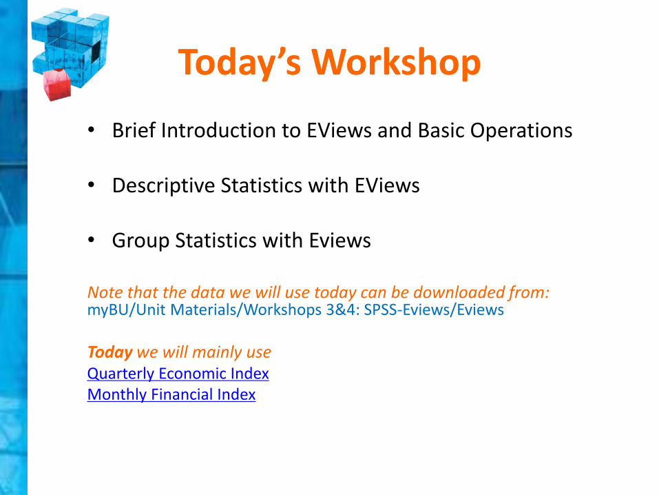
Today’s Workshop
• Brief Introduction to EViews and Basic Operations
• Descriptive Statistics with EViews
• Group Statistics with Eviews
Note that the data we will use today can be downloaded from: myBU/Unit Materials/Workshops 3&4: SPSS-Eviews/Eviews
Today we will mainly use Quarterly Economic IndexMonthly Financial Index

Brief Introduction to EViews and Basic Operations
Workfiles, objects and their basic operations Importing dataStructure your dataData operationGraphical skill Fundamental operation and function

Descriptive Statistics
Different ways of obtaining descriptive statistics for your data
Interpreting descriptive statisticsHistogramSeries Statistics

Group Statistics
CorrelationCointegrationSimple linear regression modelInterpreting the resultsIntroduction to multiple linear regression
modelling
What is Eviews (Econometrics Views) ?
EViews is an easy-to-use statistical, econometric, andeconomic modeling package, which provides data analysis,regression and forecasting tools:• Useful for many different analyses• Very user-friendly (like Windows)• Excellent help function
In this introduction workshop, we will introduce two differentways to work in EViews:• Graphical user interface (using mouse and menus/dialogs).• Single commands (using the command window).
Getting Start
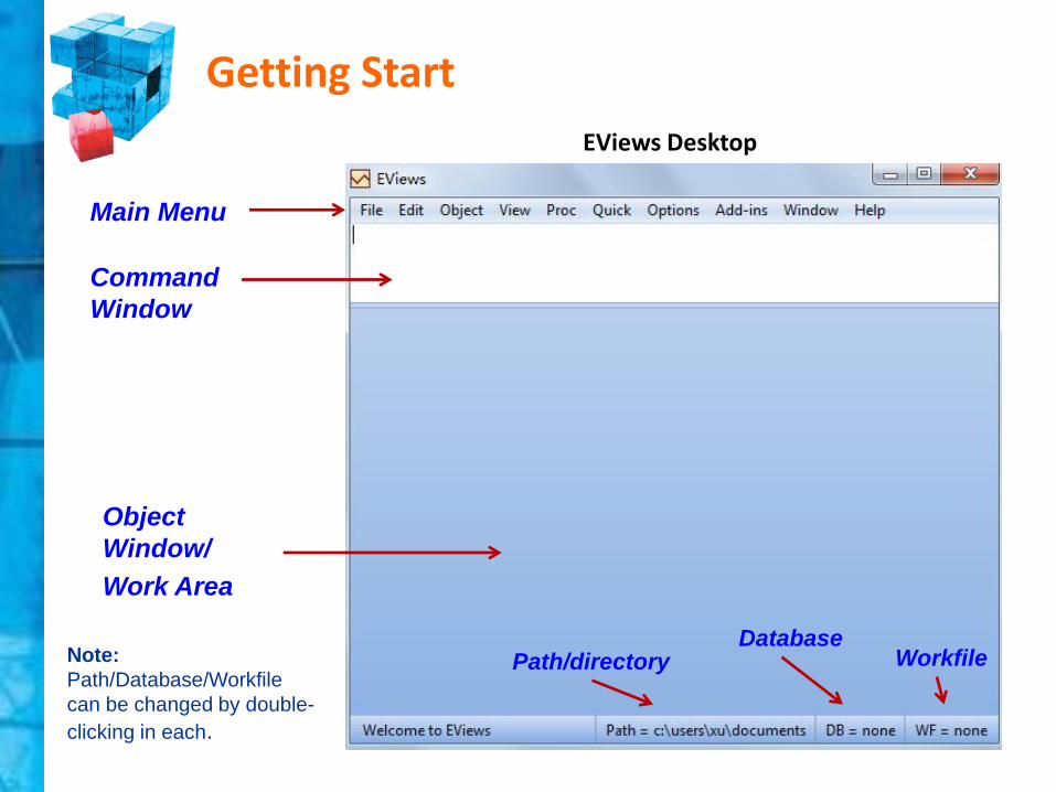
EViews Desktop
Command
Window
Object
Window/
Work Area
Main Menu
Path/directoryDatabase
WorkfileNote:
Path/Database/Workfile
can be changed by double-
clicking in each.

Workfiles and Objects
• EViews does NOT open up with a “blank” generic document (unlike Word ®, Excel ®, etc.).
• EViews documents (“workfiles”) need to be created and are not generic (they will contain information about your data, etc.).
• EViews is an “object”- oriented program. Objects are collections of information related to a particular analysis (series, groups, equations, graphs, tables).
• Workfiles are holders of these “objects”, it is the central place to keep all of your work.

Eviews Workfile
Workfile title bar
Workfile:
Contains at least one page
Each page contains a list of objects on that page
Workfile tool bar
Workfile Window

Eviews Workfile
Name of the workfile
Monthly financial index in this
example) Structure of the workfile
The data in this example is
dated and has monthly
frequency covering the
period from 1977 to 2012.
Range: shows the entire
range of the data in the
workfile. Here the range is
from M1 1977 to M11 2012
Sample: This is the part of data we are currently
working with. In this example, the sample runs
from Q1 1992 to Q4 2001.

Example Eviews Workfile and Objects
• This screenshot shows a list of Objectsin the example workfile.
• It is color-coded by Object type:
Yellow icons are data objects
Blue icons are estimation objects
Green icons are view objects (tables, graphs, etc…)
• Double clicking on one of these Object icons will open it up.
• Each Object has its own menu.
• Once an object is open, the menus in EViews change to represent the features available for that object.

Symbols of Different Types of Objects
Series, Groups
and Equations
are the most
common objects
in EViews.

The Object Window
Main menu
Workfile Toolbar
Object Toolbar
(in this example,
series toolbar)
Object Window
(in this example,
series window)

The Series Object
• This is the main data object.
• sp500 - has a yellow icon with a little line graph in it.
• It contains one column of data.
• Opening a series will reveal a spreadsheet view with a single column showing the data in the series.

The Group Object
• This is a collection of series objects.
• group01 - has a yellow icon with a capital G.
• It contains multiple columns of data.
• Opening a group will display a spreadsheet view with multiple columns showing the data in each series in the group.

Workfiles Operations
•Any work in EViews is created in workfiles – which are place-holders of EViews objects.
•Unlike other types of programs, an EViews workfilemust be created.
•Every workfile contains one or more workfile pages, each with its own objects.
•To set-up a workfile, you can either:
Create a “blank” workfile (this requires structuring);
Create a workfile by reading from a foreign source.

Creating a Workfile
• Creating a ‘’blank’’ workfile– Main menu → File→ New → Workfile
• Data Structure (Frequency, start/end dates, etc.)
The structure determines how many observations (i.e. rows)
every series in the workfile page contains. There are three general types of workfile structure:
Time Series → Dated/Regular → Frequency + Date Range
Cross-Sectional → Undated/Unstructured → Range of observations
Balanced Panel (panel data)
• Save & Name

Creating a Workfile
18
1.
2.
3.
Area 1.
Use the “Workfile structure
type” pull down menu to specify
the general structure type.
Area 2.
Use the “Date specification” area
to specify the frequency and the
start date/time and end date/time.
Area 3.
Enter a specific workfile name and
first page for the workfile.

Creating a Dated Workfile: Example 1
To create a workfile with monthly data from 1950 to 2012:
1. Click File → New → Workfile…
2. The Workfile Create dialog box
opens up.
3. Select Dated-regular frequency
from the drop-down menu of
“Workfile structure type”.
4. Select Monthly from the drop-down
menu of “Date specification”.
5. Enter the start and end date of your
data (1950 - 2012).

Creating an Undated Workfile: Example 2
1. Click File → New → Workfile
2. The Workfile Create dialog
box opens up.
3. Select Unstructured/Undated
from the drop down menu of
“Workfile structure type”.
4. Type the number of
observations in “Data Range”
(in this case 50).
To create a workfile with GDP data for all 50 states (50 observations)

Creating a Balanced Panel Workfile: Example 3
To create a Workfile Containing Quarterly Data from 1950-2010
for 100 countries
1. Click File → New → Workfile…
2. Select Balanced panel from the
drop down menu of “Workfile
structure type”.
3. Select Quarterly from the drop
down menu of “Panel
specification”.
4. Enter the start and end date of
your data (here 1950 - 2012).
5. Enter the number of cross
sections (here 100 countries).

Creating Workfiles Using Commands
Example 1Enter the following command into the command window, then press Enter
wfcreate(wf=monthly, page=dated) m 1950 2012The new workfile is named MONTHLY containing a single page named DATED, structured as a monthly workfile from 1950-2012.
Example 2Enter the following command into the command window, then press Enter
wfcreate(wf=undated, page=state) u 50The new workfile is named UNDATED containing a single page named STATE, structured as undated workfile with 50 observations.
Example 3Enter the following command into the command window, then press Enter
wfcreate(wf=panel, page=country) q 1950 2010 100The new workfile is named PANEL containing a single page named COUNTRY structured as a panel workfile with 100 cross-sections of quarterly data from 1950 - 2010.

Creating Workfiles from foreign data source
• EViews can create a new workfile by opening data from a variety of formats (Excel ®, HTML, CSV, ASCII, RATS, Stata, SPSS, SAS, etc…).
• EViews automatically recognizes the format and structure of files.
• Simply open the file in EViews and let the application do the rest.
• There are a number of ways to open a file in EViews:a) Drag/drop a file in the main EViews window (this is the easiest
method).
b) Click File → Open → Foreign Data as Workfile.
c) Copy/Paste as New Workfile in EViews desktop.

Dragging/Dropping Data: Example 1
1. The easiest way to create a workfile is to select a file and drag/drop it onto the EViews desktop.
2. A “+” (plus) “Copy” sign appears when the file is in the appropriate area.
3. The Excel Read dialog appears.
4. In most cases (including this one), clicking Finishon this dialog will load the data.
5. EViews scans the Excel file to determine the structure.
Note: If your data has lines of textbefore the column of data (showingdata sources, and other info), youcan tell EViews to skip these lines inthe Column headers section whichappears if you hit Next instead ofFinish.

Importing Data: Example 2
1. Click File → Open → Foreign Data as Workfile.
2. Select the directory where data is stored and open file.
3. The Excel Read dialogue appears again.
4. As in the previous examples, click Finish to load the data.

Copy/Paste: Example 3
1.Copy the source file (in this case the range of Excel rows) .
2.Right-click anywhere on the EViews desktop.
3.Select Paste as New Workfile.
4.As in the previous examples, the Excel Read dialog appears; click Finish to load the data.

Importing Data by Command
You can just as easily open a foreign source file in EViews bytyping in the command window.
1. Enter the following command into the commandwindow, then press Enter
wfopen(page=test) ‘’c:\test.xls’’
This creates a new workfile page named ‘’test’’. The secondpart of the command instructs Eviews where the file islocated.
2. The Excel Read dialog appears again, then click Finish toload the data.

Object Operation
• Series and Groups are the most important Data Objects in Eviews.
• The actual numeric values of your data are held in the Series Object.
• A collection of Series (multiple data columns) comprises a Group
Object.
• This section demonstrates basic work with Series and Groups:
Creating a Series
Bringing data into EViews
Creating New Series from Existing Series
Editing, documenting and displaying a Series
Creating Groups and working with Groups

Creating a New Series
Example 11. Select Object → New Object from the main
menu.
2. Click the Series option, name it (in this case series1).
3. Click OK.
Example 2Type the following command in the command window, then press Enter
series series2
Note that the new series created by either method will have the structure of the workfile and NA in all entries.

Getting Data into an Existing Workfile
Example 11.Open one of the new series with empty (NA) values we created above.
2.Click the Edit+/- button to turn on editing mode.
3.Start entering in data.
Example 21.Open the data in Excel (or other applicable applications ).
2.Highlight the series you wish to bring into Eviews and select copy (note that you do not need to copy dates since the Eviews workfile is already structured by date).
3.In EViews workfile click Quick → Empty Group (Edit Series).
4.A window opens up with a blank spreadsheet and dates on the side. Place the cursor on the upper-left cell, right-hand-click, and choose Paste.

Getting Data into an Existing Workfile
Example 3 (from foreign files)1.On the menu bar, select File (or Proc) → Import→ Import from file.
A standard File Open dialog box appears which allows you to locate the file.
2.Click Open once you locate the file. The Excel Read dialog box opens up prompting for additional information for the import procedure.
3.Click Finish to load the data.

Transforming Existing SeriesIn order to create a series y=log(sp500) Note that in Eviews, log(x) is the natural logarithm (not of base 10)
Example 1In the command window, type the following command then press Enter.
series y=log(sp500) or genr y=log(sp500)
Example 21.click Quick → Generate Series from the menu toolbar.
2.The window Generate Series by Equation opens. Type your data transformation here (in this case, x=log(sp500)).
3.Click OK.

Groups
• Groups help you work with multiple series.
• A Group is a list of series names (and potentially mathematical expressions) that provides access to all the data in that list.
• Once you create a Group Object, you can use the group name in many places to refer to all the series contained in that group.
• A few features of groups:
A group is a “live” feed and is NOT a copy of each individual series. This means that if the data in one of the series changes, these changes will also be reflected in the group containing the series.
If a series is deleted from a workfile, the series identifier will be maintained. In the group spreadsheet the deleted series will contain NA values.
Renaming a series changes the reference in every group containing the series.

Creating Groups
Example 11. Select Object → New Object from the main menu.
2. The New Object box opens up. Select the Group option.
3. You can name your group under the section Name for object (in this case, we named it group01), then press OK.
4. The Series List window appears. Enter the series names you wish to include in the group (separated by spaces).
Example 21.Select Quick → Show from the main menu (or Show from the
workfile menu).
2.The Show window appears. Type here the names of the series you wish to include in the group
3.Press OK.
4.Click Name button to save the group.
5.The Object Name box opens up, name the group here.

Creating Groups
Example 31. Highlight the series you wish to group together.
2. Right-click and select: Open → as Group.
3. As before, Click Name button to save the group.
4. The Object Name box opens up, name the group.
Example 4Type the following command in the command window, then press Enter.
group group03 tbill1y tbill3m tbill6m
This produces a group named ‘’group03’’, which includes series tbill1y, tbill3m and tbill6m.

Graphing in EViews
• Graphing is an important part of the process of data analysis and presentation.
• EViews provides a powerful, user-friendly, full-featured set of tools that will aid you in graphically displaying your information.
• Today we focus only on basic graphing in EViews. The main topics are:
Graph Options and Graph Objects
Graphing Single Series
Graphing Multiple Series

Creating a Graph1. Open series SP500.
2. Click View → Graph.
3. This brings up the Graph Optiondialog box. Under Option Pagesselect Basic type page.
4. Under the Graph type section, select Basic graph from the Generalcategory.
5. Select Line & Symbol from the Specific category.
6. Leave Details settings as specified by default options (and as shown here).
7. Click OK.
8. Click Freeze to save the graph by creating a new graph object
9. Click Name to save this new graph object
10. The Object Name box opens up, name the graph.

Graph Options Menu
The Graph Options menu is broken into several categories: 1. Option Pages: This is used for customization. 2. Graph Type: this specifies the type of graph you wish to display. It
has two categories: General and Specific General – this combo box
has two options:
o Basic graph: shows basic graph of data.
o Categorical graph: shows data divided into categories defined by factor variables
Specific: offers a list of the graph types available for use. Note that there are different options available for series and groups.
Series Groups

Graph Data – specifies the data to be used in
observation graphs
o Raw data – is the default setting. Every
observation is plotted.
o Summary Statistics – allows you to
compute summary statistics (means,
medians, etc).
For a single series, the summary
statistics shows a single data point.
For single series, you may want to
leave the setting at Raw data.
The Graph data option is more useful
with multiple series (Groups)
3. Details: this category specifies additional details, such as:
Graph Data
Orientation
Axis Borders
Multiple Series
Graph Options Menu

Orientation – allows you to choose between two options:
o Normal – observations are along the horizontal axis.
o Rotated – observations are along the vertical axis.
• Please note that for three types of graph – Distribution, Quantile-Quantile or Seasonal Graphs – different options appear instead of Orientation.
oDistribution Graphs – the Orientation option changes to Distribution with the drop-down menu shown here.
Graph Options Menu
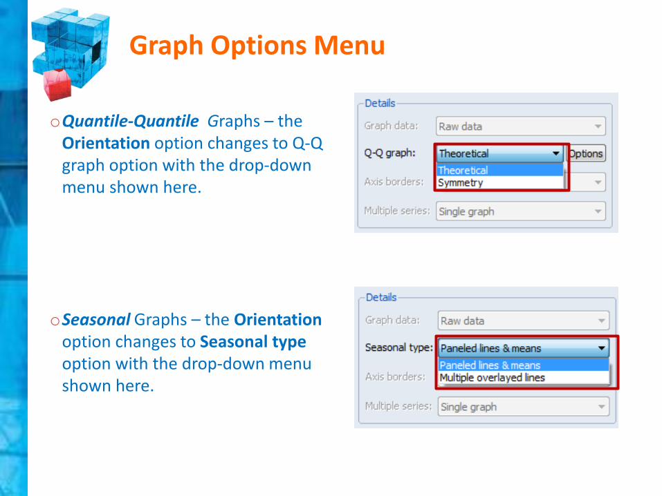
oQuantile-Quantile Graphs – the Orientation option changes to Q-Q graph option with the drop-down menu shown here.
oSeasonal Graphs – the Orientationoption changes to Seasonal type option with the drop-down menu shown here.
Graph Options Menu
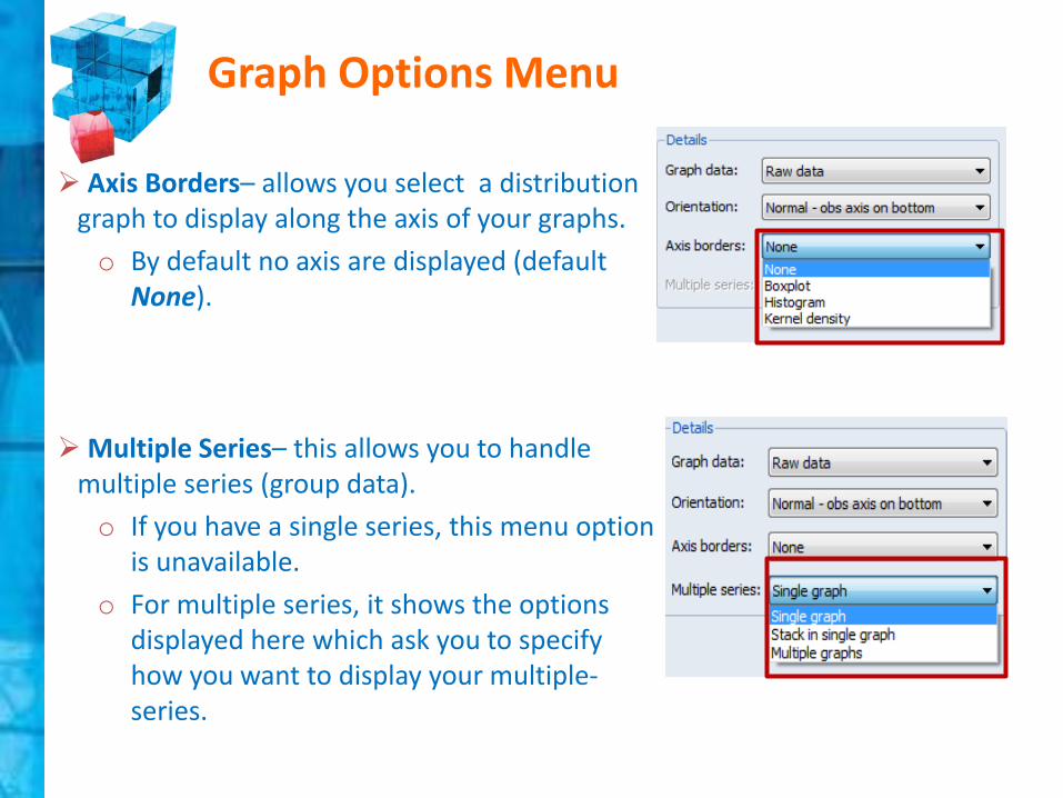
Axis Borders– allows you select a distribution graph to display along the axis of your graphs.
o By default no axis are displayed (default None).
Multiple Series– this allows you to handle multiple series (group data).
o If you have a single series, this menu option is unavailable.
o For multiple series, it shows the options displayed here which ask you to specify how you want to display your multiple-series.
Graph Options Menu

Graph Object
• When creating graphs by clicking on the Graph view from theView menu of a series or group, remember that what youcreate are simply graph views.
• These graph views are transitory: while you can customizethem, once you close the series or group object, most of thesesettings will be lost.
• You may save a graph by freezing it. This creates a graphobject.
• Freezing a view (graph object) creates a snapshot of thecurrent graph view, allowing you to create permanentcustomization of the output.

Single Series Simple Graphs
Example 1: Line & Symbol
44
• The simplest type of graph is the Line & Symbol.
• The graph shows data (as symbols, line or both) against observation identifiers.
Line & Symbol graph:
1. Open series tbill3M.
2. Click View → Graph.
3. This brings up the Graph
Option dialog box. Under
Option Pages select Basic
type page.
4. Under the Graph type
section, select Basic graph
from the General category.
5. Select Line & Symbol from
the Specific category.
6. Leave Details settings as
specified by default options
(and as shown here).
7. Click OK.
.

Single Series Simple Graphs
Example 2: Dot Plot
45
• The dot plot is a symbol-only version of the Line & Symbol graph.
• The graph uses circles to represent the value of each observation.
Dot Plots:
1. Open series tbill3m.
2. Follow steps 2-4 of Example 1.
3. Select Dot Plot from the
Specific category.
4. Leave Details settings as
specified by default options
(make sure Raw Data is
selected under Details/Graph
Data).
5. Click OK.
• The graph is shown here. .

Single Series Simple Graphs
Example 3: Bar Graph
• Bar Graphs use bars to represent the value of each observation.
• Bar Graphs are effective when there are few observations: for large numbers,
Bar Graphs and Area Graphs are almost indistinguishable from each other.
Bar Graphs:
1. Open series tbill3m.(choose
sample1977m01 to 1978m01)
2. Follow steps 2-4 shown in Example
1.
3. Select Bar (from Graph
type/Specific).
4. Leave Details settings as specified
by default options (make sure Raw
Data is selected under
Details/Graph Data).
5. Click OK. .

Single Series Simple Graphs
Example 4: Spike Plots
• Spike Plots use a thin bar to represent the value of each observation.
• Spike Plots are essentially Bar Graphs (with thin bars) and can be used to
display a moderate amount of observations.
Spike Plots:
1. Open series tbill3m.
Remember the sample is still
set in 1977m01 to 1978m01)
2. Follow steps 2-4 shown in
Example 1.
3. Select Spike (from Graph
type/Specific).
4. Leave Details settings as
specified by default options
(make sure Orientation is set
on Normal and Axis borders
on None).
5. Click OK.

Single Series Simple Graphs
Example 5: Area Plots
• An Area Graph is a line graph with the area underneath the line filled in.
Area Graphs:
1. Click on the Panel page.
2. Let’s first create a new series by
subtracting its own mean from the
tbill3m series. For this, type in the
command window:
series newseries=tbill3m-
@mean(tbill3m)
3. After creating it, now open the
series newseries. Follow steps 2-
4 shown in Example 1.
4. Select Area (from Graph
type/Specific).
5. Click OK.

Multiple Series Simple Graphs
49
• All types of graphs available for a single
series are also available for graphing
series in a group.
• Multiple Series have all the graph
options of Single series along with a few
additional ones.
• One important difference is that multiple
series graphing has one additional
option to choose that all plots in single
graph or in multiple graphs separately.
If you open a group of series, the
following graph types appear:

Multiple Series Simple Graphs
Example 1: Line & Symbol -- One Graph
Line & Symbol – One Graph:
1. Open group01.
2. Click View → Graph.
3. This brings up the Graph
Option dialog box. The
default is set on Basic
type page; keep the
default setting.
4. Under the Graph type
section, select Basic
graph from the General
category.
5. Select Line & Symbol
from the Specific
category.
6. Notice that now under
Details/Multiple Series
you have a few options.
Let’s select Single Graph.
7. Click OK.
Multiple Series Simple Graphs
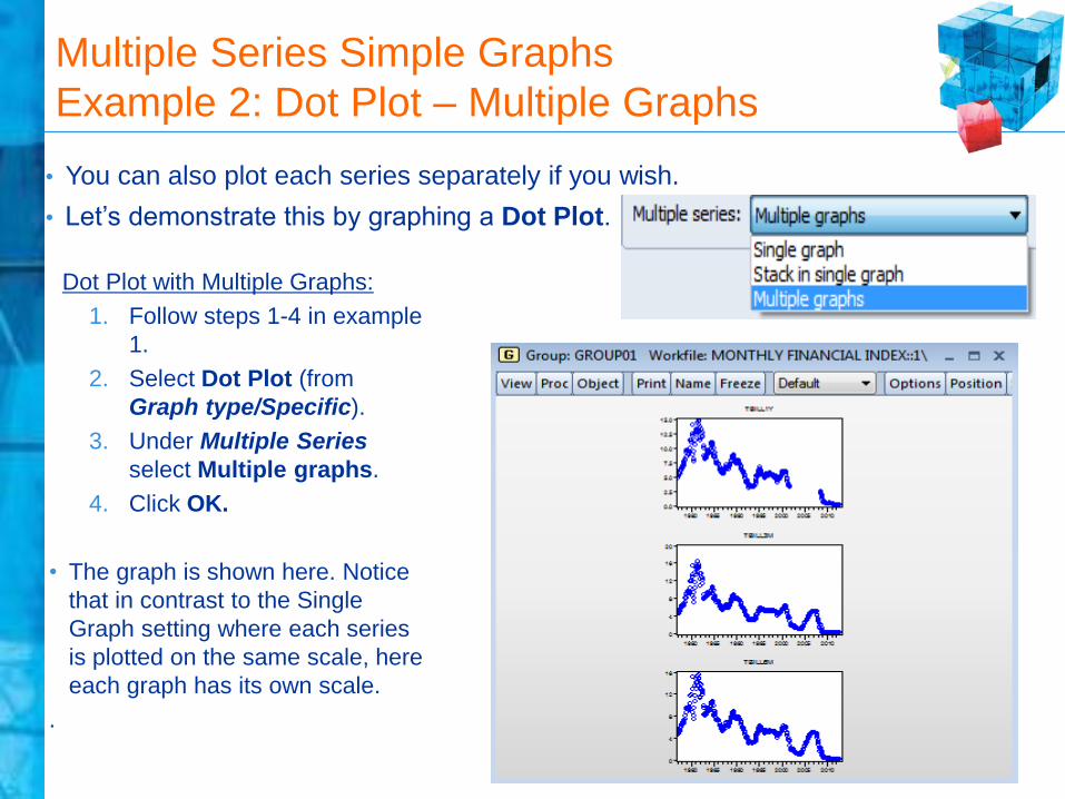
Example 2: Dot Plot – Multiple Graphs
51
• You can also plot each series separately if you wish.
• Let’s demonstrate this by graphing a Dot Plot.
Dot Plot with Multiple Graphs:
1. Follow steps 1-4 in example
1.
2. Select Dot Plot (from
Graph type/Specific).
3. Under Multiple Series
select Multiple graphs.
4. Click OK.
• The graph is shown here. Notice
that in contrast to the Single
Graph setting where each series
is plotted on the same scale, here
each graph has its own scale.
.

Multiple Series Simple Graphs
Example 3: Area Plot – Stack in One Graph
Area Plot – Stack in One Graph:
1. Follow steps 1-4 in example 1.
2. Select Area (from Graph
type/Specific).
3. Under Multiple Series select
Stack in single graph.
4. Click OK.
• The graph is shown here. Notice
that here the first series (tbill1y)
is plotted in the usual way. The
second series (tbill3m) is the sum
of the first and the second series.
The third series (tnote6m) is the
sum of the first three series, etc..
• You can also stack your series in a single graph. This sums the values of each
series vertically.
• Let’s demonstrate this by graphing an Area Plot.

Multiple Series Simple Graphs
Example 4: Bar Graph – Summary Statistics
Bar Graph – Means:
1. Follow steps 1-4 in example
1.
2. Select Bar (from Graph
type/Specific).
3. Under Graph data select
Means.
4. Click OK.
• The graph is shown here. Each
bar represents the mean of
each series.
• With multiple series it makes sense to take a look at summary statistics (means,
median etc.)
• Let’s plot the means of each series using a Bar Graph.

Descriptive Statistics in EViews
• The main data analysis item in EViews is the View menu.
• You can view all available actions for a series from this menu.
View menu:
1. Open one series
2. Click on the View menu item. A drop-
down menu appears with a number of
options grouped in 4 sections.
The first section/block lists views
that display the data series.
The second bloc provides general
statistics.
The third block provides general
statistics for time series.
The fourth block allows you to
modify/display the series labels.

Histogram and Stats
• Basic statistical summaries (including histograms) can be found in EViews
under the View → Descriptive Statistics & Tests
Descriptive Statistics: Histogram
1. Open one series
2. Click View →Descriptive Statistics & Tests → Histogram and Stats.

Histogram and Stats
The table of the right side will show if you click View →Descriptive Statistics & Tests →
Stats Table.(this is easy to copy and paste into a word processor or spreadsheet program)
1. The top of the statistics panel shows the name of the series, the sample(only for
Histogram and Stats ) , and the number of observations (bottom of Stats Table).
2. In the middle, EViews summarizes the main statistics for the GDP series.
(note: skewness measures the degree of asymmetry in data, where as kurtosis measures
the presence of “fat tails”).
3. The bottom of the panel shows the Jarque-Bera statistic and its associated probability
and tests whether the data is drawn from a normal distribution. Since here, the p-value is
0.0048, it is extremely unlikely that the data follows a normal distribution.

One-Way Tabulation
• If you want to see the entire distribution of the data, you can do so by using
One-Way Tabulation.
1. First, make sure you include all
observations in the workfile by
typing in the command window:
smpl @all
2. Open series GDP
3. Click View → One-Way
Tabulation. The Tabulate Series
dialog box opens up. Let’s
uncheck the boxes under the
section “Group into bins if.”
4. The tabulation is shown here. As
you can see, EViews provides
the counts, percentage counts
and cumulative counts for each
observation value.

View Menu for Groups
View menu for Groups:
1. Highlight series g gdp and inv, right
click and select Open → as Group.
2. Click on the View menu item. A
drop-down menu appears with a
number of options grouped in 4
sections.
The first section/block provides
various ways of looking at the
data in the group.
The second bloc provides general
statistics.
The third block provides general
statistics for time series.
The fourth block allows you to
modify/display the group labels.

• Basic statistical summaries of the series contained in one group can be
found in EViews under the View → Descriptive Statistics.
Descriptive Statistics:
Common / Individual Sample
1. Open group01.
2. Click View → Descriptive Statistics →
Common / Individual Sample.
• General stats for all the series in the
sample are shown here. Note that
statistics are computed using a
common sample. This means that if a
series has missing observations, stats
for all series are computed over the
common sample for which all series
have non-missing observations.
• You can also compute Descriptive
Statistics for the series in one group
over the sample of each individual
series.
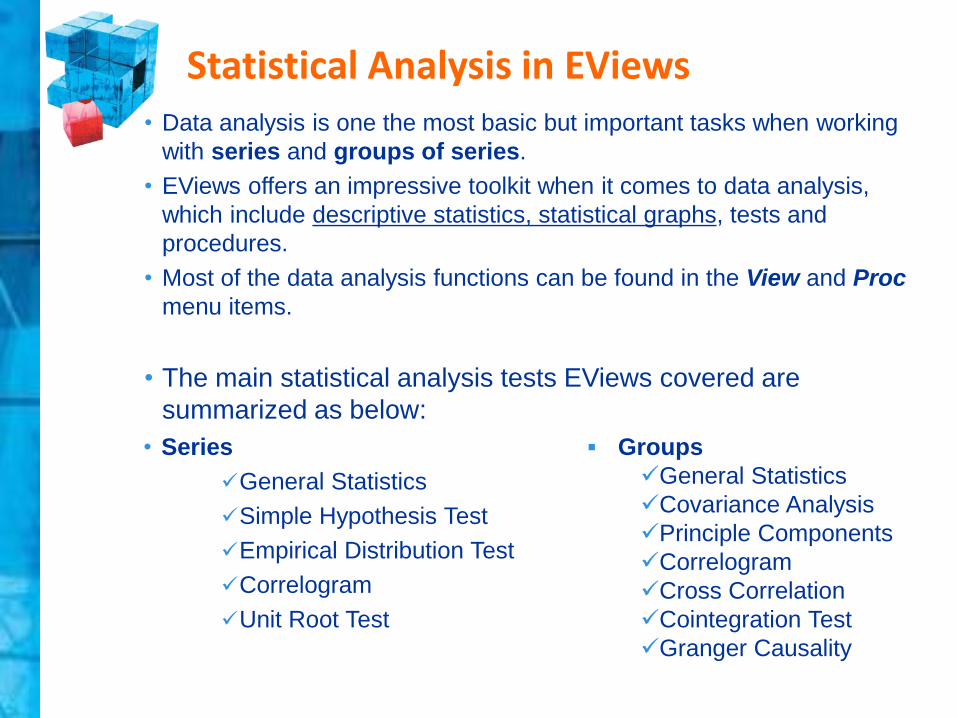
Statistical Analysis in EViews• Data analysis is one the most basic but important tasks when working
with series and groups of series.
• EViews offers an impressive toolkit when it comes to data analysis,
which include descriptive statistics, statistical graphs, tests and
procedures.
• Most of the data analysis functions can be found in the View and Proc
menu items.
• The main statistical analysis tests EViews covered are
summarized as below:
• Series
General Statistics
Simple Hypothesis Test
Empirical Distribution Test
Correlogram
Unit Root Test
Groups
General Statistics
Covariance Analysis
Principle Components
Correlogram
Cross Correlation
Cointegration Test
Granger Causality
Running Regression in EViews
The main topics include:
Specifying and estimating an equation
Equation Objects (saving, labeling, freezing)
Equation Output: analyzing and Interpreting results
Basic Multiple Regression Analysis

Equation Object
• Single equation regression estimation in EViews is performed using the
Equation Object.
There are a number of ways to create a simple OLS Equation Object:
1. From the Main menu,
select Object → New
Object → Equation.
2. From the Main menu, select Quick →
Estimate Equation.
3. On the command window type: ls

Equation Estimation Box
Specify your equation either by:
a) List
b) Formula
Specify your estimation method
(more methods in dropdown menu)
Specify your sample
In all cases after the previous step, the Equation Estimation box appears.
You need to specify three things in this dialogue box:
1. The equation specification.
2. The estimation method.
3. The sample.

Specifying an Equation
You can create an Equation simply by selecting the series and opening them as Equation.
1. Select employment_retail,
tnote10y and tnote2y by
clicking on these series in the
workfile (press CTRL to select
multiple series). Notice that
you need to select the
independent variable first.
2. Right click and select Open →
as Equation.

Specifying an EquationIn the Equation Estimation dialogue box, you can type in the Equation specification boxto specify your equation (same as the previous example):
employment_retail c tnote10y tnote2y
Note that always dependent variable first, followed by list of independent variables andconstant term c.
OR in the command window by typing in the following command then press Enter:
ls employment_retail c tnote10y tnote2y

Regression Output
• All previous methods will finally give
you the estimation output in
equation object.
• Click the Name button to name and
save the equation object.
• Freeze the results will save the
equation output in a table which will
never change.
• The Equation box has three main
parts, which we will discuss in turn:
1. The top panel summarizes the
input for the regression.
2. The middle panel summarizes
information about regression
coefficients.
3. The bottom panel provides
summary statistics about the
entire regression.
Top Panel
Middle Panel
Bottom Panel

Element Description
Dependent Variable Denotes the dependent variables.
Method Denotes the method of estimation (least squares in this
example).
Date/Time Shows the date and time when the regression was carried out.
Sample Shows the sample period over which the regression is carried out.
Included
Observation
Shows the number of observations included in estimation.
Coefficient Values • measures the marginal contribution of independent variable todependent variable.
• C is the estimated constant (or intercept) of the regression.
Standard Errors • Reports the standard errors of the coefficient estimates.• The larger the standard errors, the more noisy the estimates.
t-Statistic • Reports the t-statistics, computed by dividing coefficient estimates by their standard errors.
• Is used to test whether the coefficient in that row equals zero.
Prob. (p-value) • Reports probability of drawing a t-statistic as extreme as the one actually estimated.
• Is used to test whether the coefficient is equal to zero (against a two-sided alternative).
Regression Output

Regression Output
Statistic Description
R-squared Measures the success of the regression in predicting the values
of depended variable.
Adjusted R-
squared
Adjusts for the number of independent regressors by penalizing
R-squared for additional regressors.
S.E. of regression Is a summary measure based on estimated variance of the
residuals.
Sum squared
resid
Reports the sum of squared residuals. The same as (S.E. of
regression)2 * (T-k-1), where T is the number of observations, k is
the number of independent variables.
Log-likelihood Reports the log likelihood function evaluated at coefficient
estimates assuming normally distributed errors.
F-statistic Tests whether all slope coefficients (excluding the constant) are
zero.
Prob(F-Static) Reports the probability of drawing an F-statistics as the one
estimated.
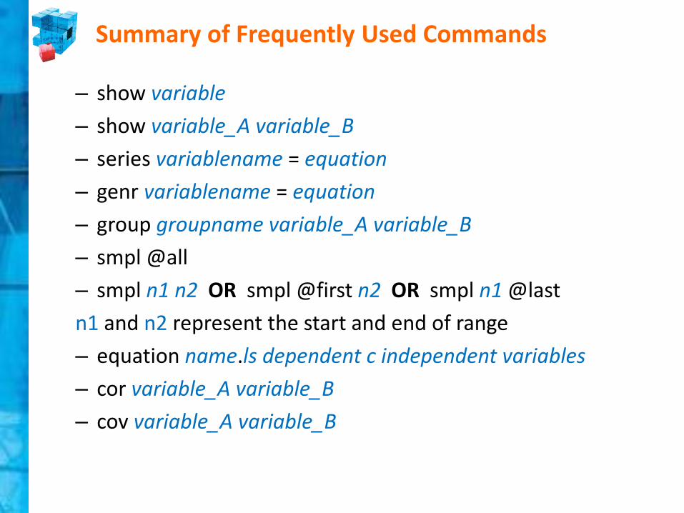
Summary of Frequently Used Commands
– show variable
– show variable_A variable_B
– series variablename = equation
– genr variablename = equation
– group groupname variable_A variable_B
– smpl @all
– smpl n1 n2 OR smpl @first n2 OR smpl n1 @last
n1 and n2 represent the start and end of range
– equation name.ls dependent c independent variables
– cor variable_A variable_B
– cov variable_A variable_B

Thanks for your attention!
Website: microsites.bournemouth.ac.uk/mathssupport/

Fundamental Operation and Functions
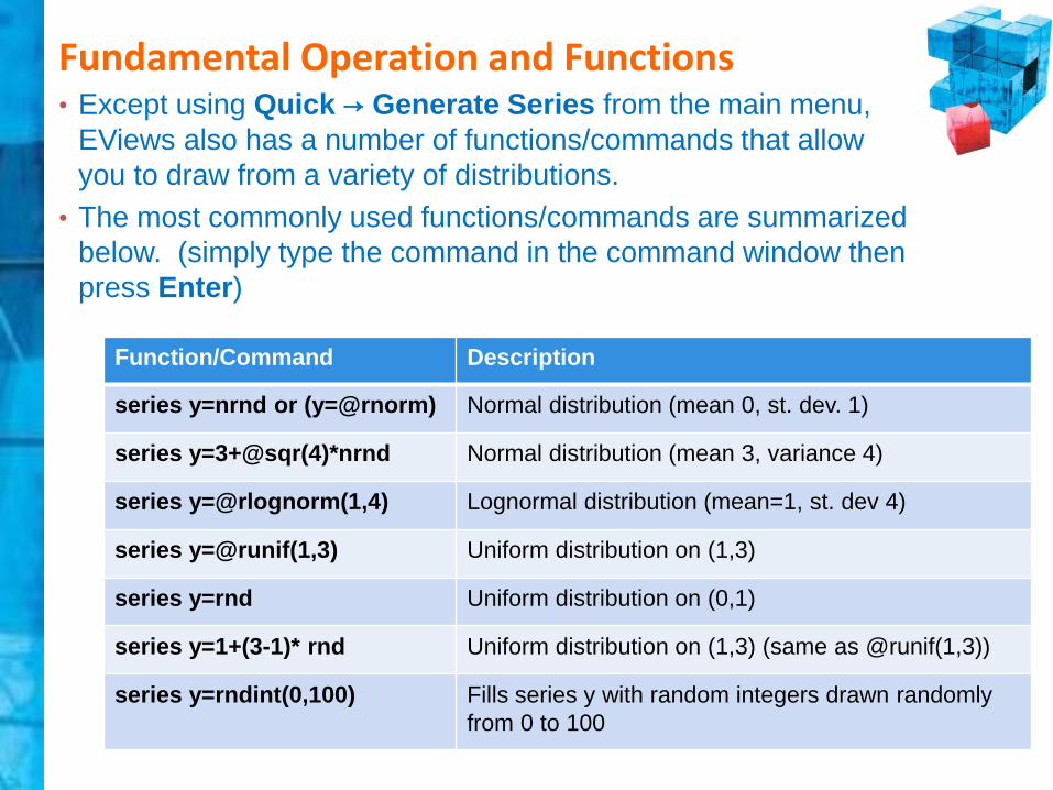
Function/Command Description
series y=nrnd or (y=@rnorm) Normal distribution (mean 0, st. dev. 1)
series y=3+@sqr(4)*nrnd Normal distribution (mean 3, variance 4)
series y=@rlognorm(1,4) Lognormal distribution (mean=1, st. dev 4)
series y=@runif(1,3) Uniform distribution on (1,3)
series y=rnd Uniform distribution on (0,1)
series y=1+(3-1)* rnd Uniform distribution on (1,3) (same as @runif(1,3))
series y=rndint(0,100) Fills series y with random integers drawn randomly
from 0 to 100
• Except using Quick → Generate Series from the main menu,
EViews also has a number of functions/commands that allow
you to draw from a variety of distributions.
• The most commonly used functions/commands are summarized
below. (simply type the command in the command window then
press Enter)

Time Series Functions
Type Function Description
Lags & leads
gdp(-4) Denotes the 4th lag of the GDP series
gdp(2) Denotes the 2nd lead of the GDP series
gdp (-1 to -4) Specifies all GDP lags from 1 to 4
gdp(to -5) OR gdp (0 to -5) Specifies all GDP lags from 0 to -5
series y = @lag(gdp,3) Generates series y, as the 3rd lag of GDP
series y =@lag((gdp-
inv)/gdp,4)
Generates series y, as the 4th lag of the
transformation (gdp-inv)/gdp
Differences
d(gdp) = gdp - gdp(-1) Takes the first difference of the GDP series
d(gdp,3) 3rd order difference of GDP series
dlog(gdp) = log(gdp) – log(gdp(-1)) Takes the first difference of log(GDP) series
dlog(gdp,4) 4th order difference of log(GDP) series
Trend
@trend Time trend increasing with each observation
@trend^2 Quadratic time trend increasing with each
observation
Common Commands/Functions
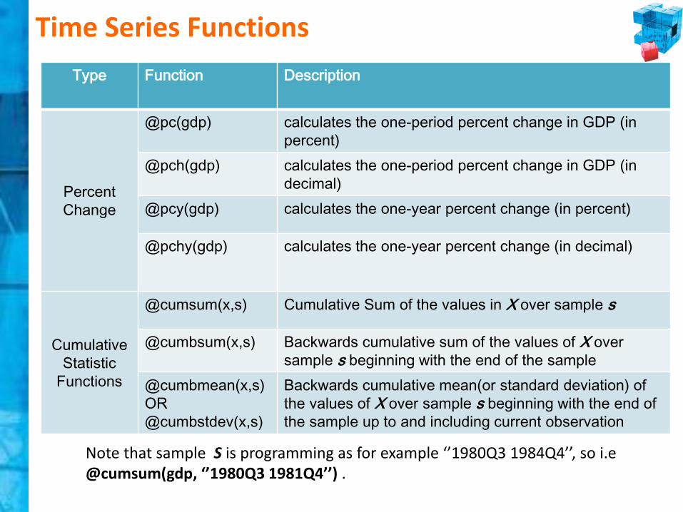
Type Function Description
Percent
Change
@pc(gdp) calculates the one-period percent change in GDP (in
percent)
@pch(gdp) calculates the one-period percent change in GDP (in
decimal)
@pcy(gdp) calculates the one-year percent change (in percent)
@pchy(gdp) calculates the one-year percent change (in decimal)
Cumulative
Statistic
Functions
@cumsum(x,s) Cumulative Sum of the values in X over sample s
@cumbsum(x,s) Backwards cumulative sum of the values of X over
sample s beginning with the end of the sample
@cumbmean(x,s)
OR
@cumbstdev(x,s)
Backwards cumulative mean(or standard deviation) of
the values of X over sample s beginning with the end of
the sample up to and including current observation
Time Series Functions
Note that sample S is programming as for example ‘’1980Q3 1984Q4’’, so i.e@cumsum(gdp, ‘’1980Q3 1981Q4’’) .

Empirical Distribution TestsEViews can carry out a number of empirical distribution tests, which test
whether the data generating process for our series comes from one of these
distributions:
Hypothesis Tests: Example 4
1. Open GDP series. Click View →
Descriptive Statistics & Tests →
Empirical Distribution Tests.
2. The EDF Test dialog box opens up. There
are two tabs:
Test Specification – allows you to
specify the parametric distribution
against which you want to test the
empirical distribution of the series.
Estimation Options – provides control
over any iterative estimation performed.
This tab is mostly used in those cases
when there is a failure in the estimation
process. Otherwise you won’t need to
use this particular tab.
3. Under the Parameters section you can
specify the values of any known
parameters. If you leave it blank, EViews
will estimate these from your data.
4. Click OK.

Descriptive Statistics-FunctionsEViews has extensive built-in descriptive statistical functions and the
common commands/functions are summarized as follows:
Function Description
series y=@gmean(x) Computes the geometric average of X
series y=@mean(x) Creates a series where each observation is equal to the
mean of X
series
y=@mean(x,“1980m01
1990m12”)
Creates a series where each observation is equal to the
mean of X for the defined sample (1980m01 to 1990m12)
series y=@median(x) Creates a series where each observation is equal to the
median of X
series y=@vars(x) Computes the sample variance of X (adj. by n-1)
series y=@varp(x) or
y=@var(x)
Computes the population variance of X (adj. by n)
series y=@stdev(x) or
y=@stdevs(x)
Computes the sample st. dev. of X (adj. by n-1)
series y=@stdevp(x) Computes the population st. dev. of X (adj. by n)

1. Open group02.
2. Click View → Covariance Analysis.
The Covariance Analysis dialog box
opens up. Under Method, click the
drop-down menu choose the type of
measure (let’s select Ordinary here).
3. Click the Covariance box (the
default).
4. Under Saved results basename,
name your results so they are saved
in the workfile (here cov1)
5. Click OK.
• The Covariance Analysis view is a very useful tool to obtain different measures
of association (covariance/correlation) for the series in a group.
• There are four general classes in EViews from which you can compute
measures of association: ordinary (Pearson), ordinary uncentered,
Spearman rank-order, and Kendall’s tau-a and tau-b.
Covariance Analysis