Research Highlights: Michigan State University

MURI Project Review

Santa Fe NM

11 December 2017

Mark M. Meerschaert

University Distinguished Professsor

Department of Statistics and Probability

Michigan State University

mcubed@stt.msu.edu

http://www.stt.msu.edu/users/mcubed

Research Area 1: Theory of non-local operators

• Zolotarev fractional derivative

• Nonlocal Dirichlet boundary conditions

• Duality for tempered fractional diffusion

• PhD project: Fractional calculus and turbulence

• PhD project: Fractional phase field model of failure

Area 2: Numerical solution of fractional PDEs

• Petrov-Gelerkin spectral methods (update)

• Fractional Neumann boundary conditions

• Open problem: Fractional Neumann BC in higher dimensions

• Open problem: Numerical methods for Zolotarev derivative

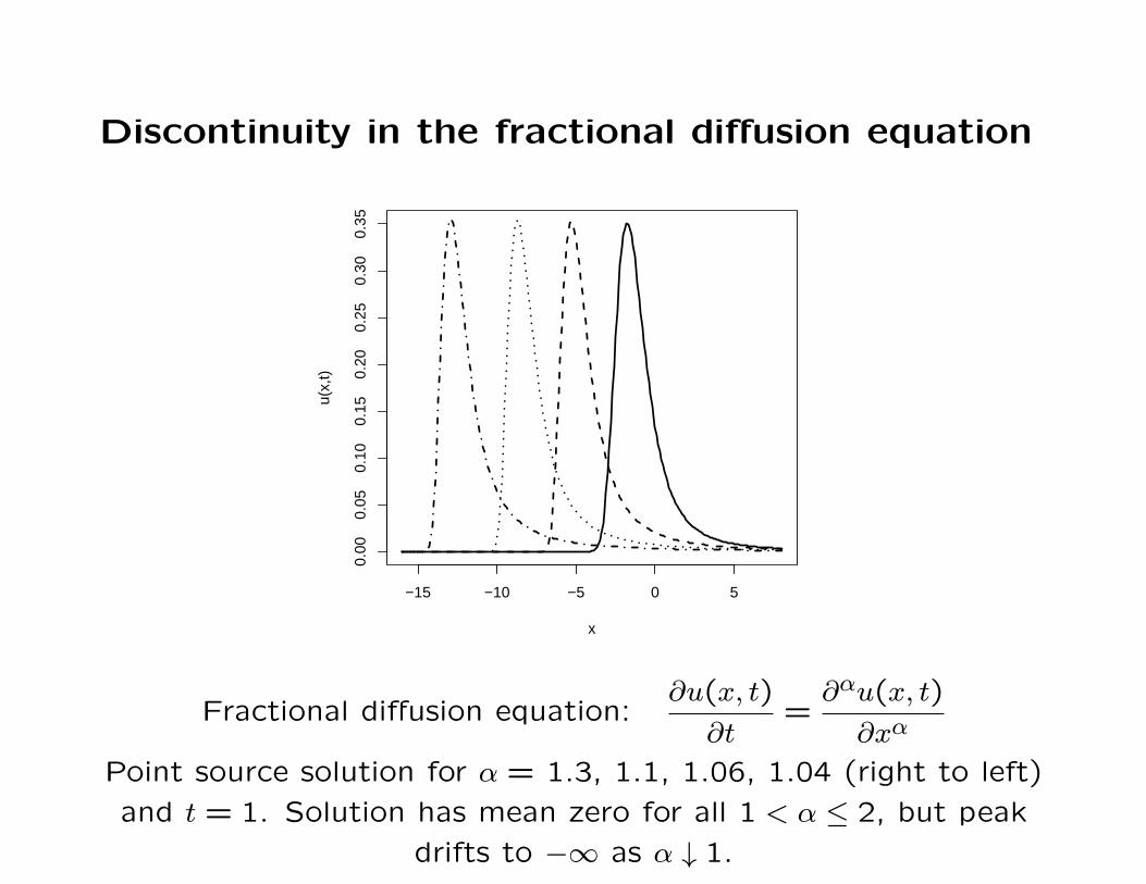
Discontinuity in the fractional diffusion equation

−15 −10 −5 0 5

0.00

0.05

0.10

0.15

0.20

0.25

0.30

0.35

x

u(x,

t)

Fractional diffusion equation:∂u(x, t)

∂t=

∂αu(x, t)

∂xα

Point source solution for α = 1.3, 1.1, 1.06, 1.04 (right to left)

and t = 1. Solution has mean zero for all 1 < α ≤ 2, but peak

drifts to −∞ as α ↓ 1.

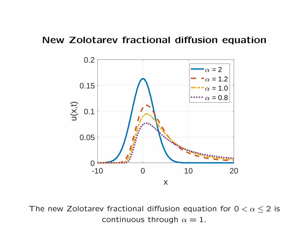
New Zolotarev fractional diffusion equation

-10 0 10 20x

0

0.05

0.1

0.15

0.2

u(x,

t) = 2 = 1.2 = 1.0 = 0.8

The new Zolotarev fractional diffusion equation for 0 < α ≤ 2 is

continuous through α = 1.

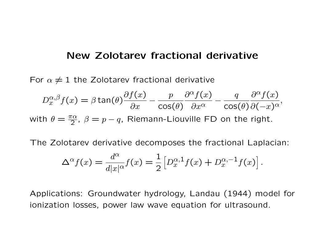
New Zolotarev fractional derivative

For α 6= 1 the Zolotarev fractional derivative

Dα,βx f(x) = β tan(θ)

∂f(x)

∂x−

p

cos(θ)

∂αf(x)

∂xα−

q

cos(θ)

∂αf(x)

∂(−x)α,

with θ = πα2 , β = p− q, Riemann-Liouville FD on the right.

The Zolotarev derivative decomposes the fractional Laplacian:

∆αf(x) =dα

d|x|αf(x) =

1

2

[

Dα,1x f(x) +Dα,−1

x f(x)]

.

Applications: Groundwater hydrology, Landau (1944) model for

ionization losses, power law wave equation for ultrasound.

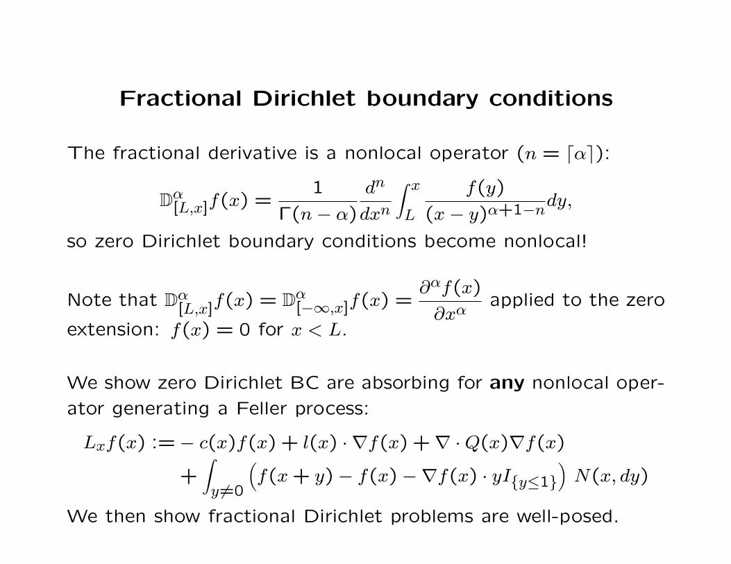
Fractional Dirichlet boundary conditions

The fractional derivative is a nonlocal operator (n = ⌈α⌉):

Dα[L,x]f(x) =

1

Γ(n− α)

dn

dxn

∫ x

L

f(y)

(x− y)α+1−ndy,

so zero Dirichlet boundary conditions become nonlocal!

Note that Dα[L,x]

f(x) = Dα[−∞,x]f(x) =

∂αf(x)

∂xαapplied to the zero

extension: f(x) = 0 for x < L.

We show zero Dirichlet BC are absorbing for any nonlocal oper-

ator generating a Feller process:

Lxf(x) :=− c(x)f(x) + l(x) · ∇f(x) +∇ ·Q(x)∇f(x)

+∫

y 6=0

(

f(x+ y)− f(x)−∇f(x) · yI{y≤1}

)

N(x, dy)

We then show fractional Dirichlet problems are well-posed.

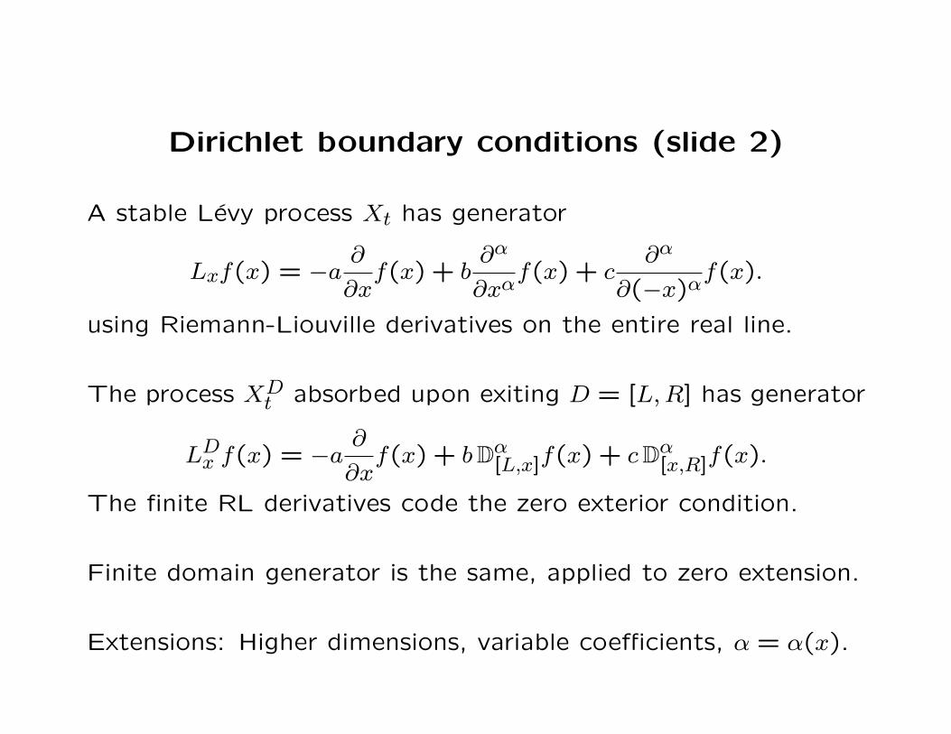
Dirichlet boundary conditions (slide 2)

A stable Levy process Xt has generator

Lxf(x) = −a∂

∂xf(x) + b

∂α

∂xαf(x) + c

∂α

∂(−x)αf(x).

using Riemann-Liouville derivatives on the entire real line.

The process XDt absorbed upon exiting D = [L,R] has generator

LDx f(x) = −a

∂

∂xf(x) + bDα

[L,x]f(x) + cDα[x,R]f(x).

The finite RL derivatives code the zero exterior condition.

Finite domain generator is the same, applied to zero extension.

Extensions: Higher dimensions, variable coefficients, α = α(x).

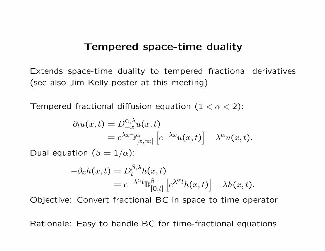
Tempered space-time duality

Extends space-time duality to tempered fractional derivatives

(see also Jim Kelly poster at this meeting)

Tempered fractional diffusion equation (1 < α < 2):

∂tu(x, t) = Dα,λ−x u(x, t)

= eλxDα[x,∞]

[

e−λxu(x, t)]

− λαu(x, t).

Dual equation (β = 1/α):

−∂xh(x, t) = Dβ,λt h(x, t)

= e−λαtDβ[0,t]

[

eλαth(x, t)

]

− λh(x, t).

Objective: Convert fractional BC in space to time operator

Rationale: Easy to handle BC for time-fractional equations

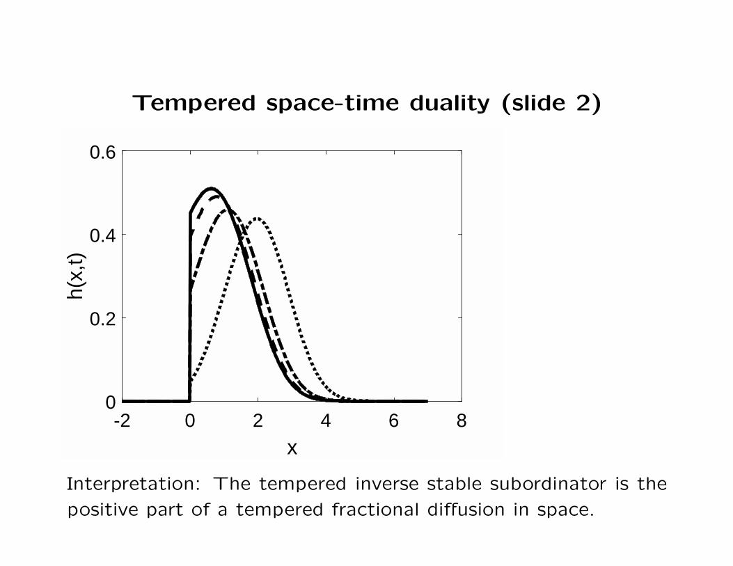
Tempered space-time duality (slide 2)

-2 0 2 4 6 8x

0

0.2

0.4

0.6

h(x,

t)

Interpretation: The tempered inverse stable subordinator is the

positive part of a tempered fractional diffusion in space.

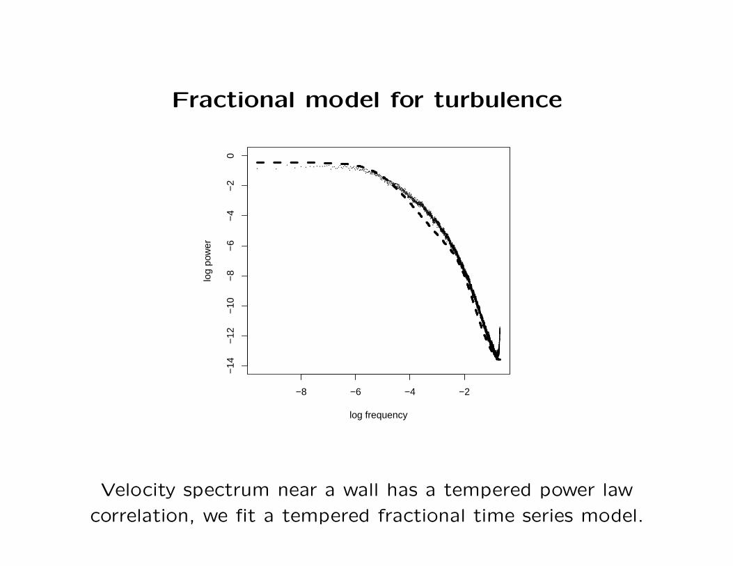
Fractional model for turbulence

−8 −6 −4 −2

−14

−12

−10

−8

−6

−4

−2

0

log frequency

log

pow

er

Velocity spectrum near a wall has a tempered power law

correlation, we fit a tempered fractional time series model.

Tempered fractional Navier-Stokes

Replace Laplacian ∆ with fractional Laplacian ∆α

Replace time derivative with (tempered) fractional derivative

Model passive scalar transport

Particle tracking using stable processes

Second part of PhD for Mehdi Samiee

Fractional phase field modeling

Reconsider phase field equations for material failure

Empirical observations of power law Energy spectrum

Investigate fractional phase field modeling

Perform relevant uncertainty quantification

PhD project for Eduardo de Moraes

Area 2: Numerical solution of fractional PDEs

• Petrov-Gelerkin spectral methods (update)

• Fractional Neumann boundary conditions

• Open problem: Fractional Neumann BC in higher dimensions

• Open problem: Numerical methods for Zolotarev derivative

Petrov-Gelerkin spectral methods (update)

Space-time diffusion in d dimensions with zero Dirichlet BC.

Jacobi poly-fractonomials are temporal basis/test functions.

Legendre polynomials are spatial basis/test functions.

Numerical implementation for fast linear solver.

Stability and error analysis.

Two papers were revised and resubmitted to the Journal of Com-

putational Physics.

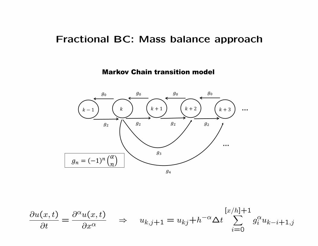
Fractional BC: Mass balance approach

+ 1 + 2 + 31 …

…

= 1

Markov Chain transition model

∂u(x, t)

∂t=

∂αu(x, t)

∂xα⇒ uk,j+1 = ukj+h−α∆t

[x/h]+1∑

i=0

gαi uk−i+1,j

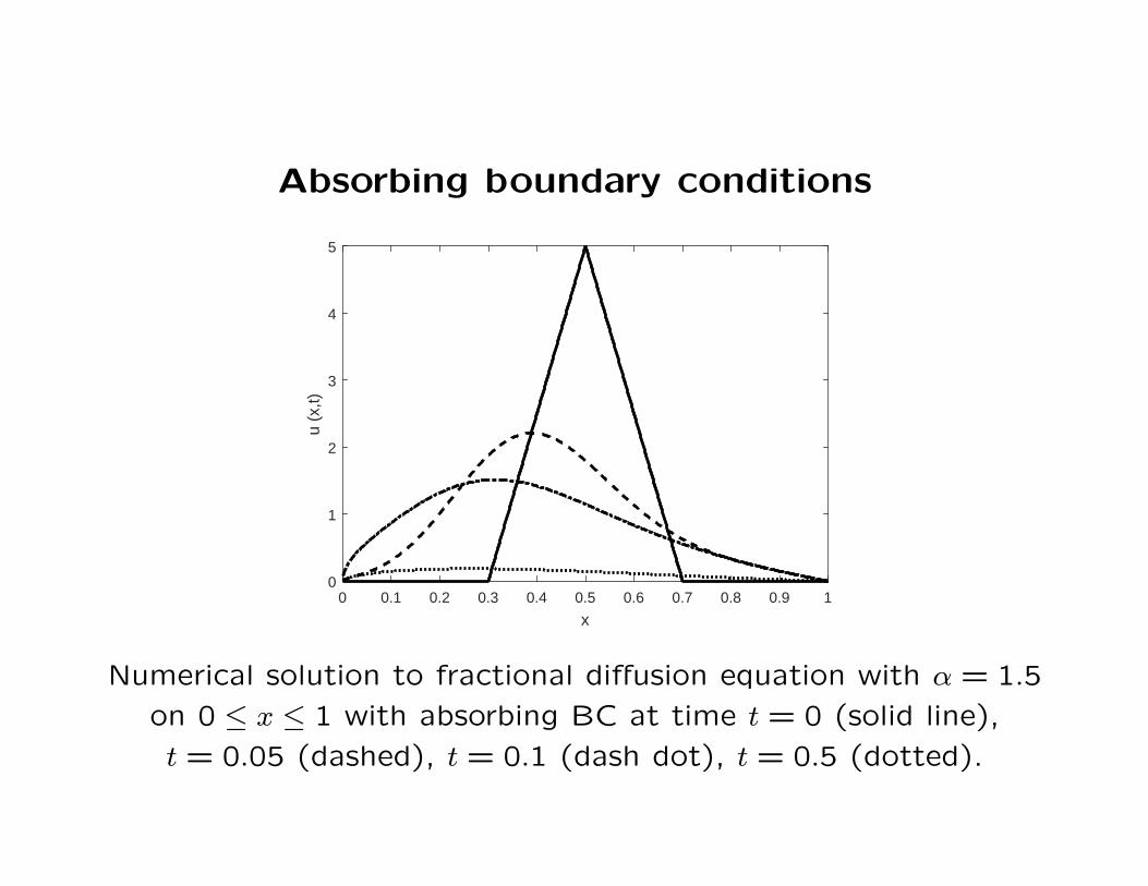
Absorbing boundary conditions

0 0.1 0.2 0.3 0.4 0.5 0.6 0.7 0.8 0.9 1

x

0

1

2

3

4

5

u (x

,t)

Numerical solution to fractional diffusion equation with α = 1.5

on 0 ≤ x ≤ 1 with absorbing BC at time t = 0 (solid line),

t = 0.05 (dashed), t = 0.1 (dash dot), t = 0.5 (dotted).

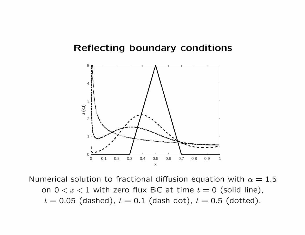
Reflecting boundary conditions

0 0.1 0.2 0.3 0.4 0.5 0.6 0.7 0.8 0.9 1

x

0

1

2

3

4

5

u (x

,t)

Numerical solution to fractional diffusion equation with α = 1.5

on 0 < x < 1 with zero flux BC at time t = 0 (solid line),

t = 0.05 (dashed), t = 0.1 (dash dot), t = 0.5 (dotted).

Fractional Neumann boundary conditions

The reflecting boundary conditions are written as

∂α−1

∂xα−1u(0, t) = 0 and

∂α−1

∂xα−1u(1, t) = 0.

This is a zero flux BC because

∂α

∂xαu(x, t) =

∂

∂x

∂α−1

∂xα−1u(x, t) = −

∂

∂xq(x, t)

where the flux q(x, t) = −∂α−1

∂xα−1u(x, t).

When α = 2 this reduces to the usual first derivative condition.

The steady state solution is u(x, t) = (α− 1)xα−2 on 0 < x < 1.

This solution has zero flux for all 0 < x < 1.

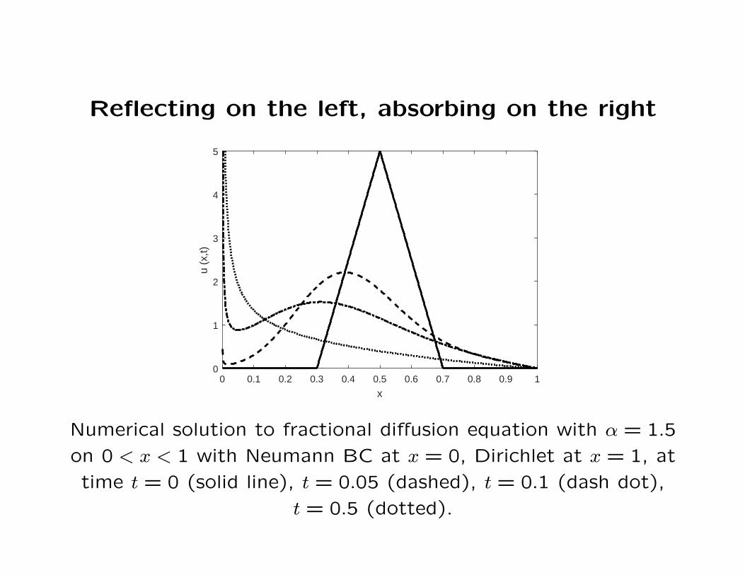
Reflecting on the left, absorbing on the right

0 0.1 0.2 0.3 0.4 0.5 0.6 0.7 0.8 0.9 1

x

0

1

2

3

4

5

u (x

,t)

Numerical solution to fractional diffusion equation with α = 1.5

on 0 < x < 1 with Neumann BC at x = 0, Dirichlet at x = 1, at

time t = 0 (solid line), t = 0.05 (dashed), t = 0.1 (dash dot),

t = 0.5 (dotted).

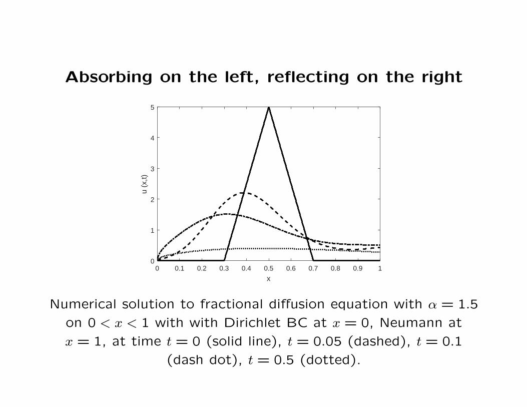
Absorbing on the left, reflecting on the right

0 0.1 0.2 0.3 0.4 0.5 0.6 0.7 0.8 0.9 1

x

0

1

2

3

4

5

u (x

,t)

Numerical solution to fractional diffusion equation with α = 1.5

on 0 < x < 1 with with Dirichlet BC at x = 0, Neumann at

x = 1, at time t = 0 (solid line), t = 0.05 (dashed), t = 0.1

(dash dot), t = 0.5 (dotted).

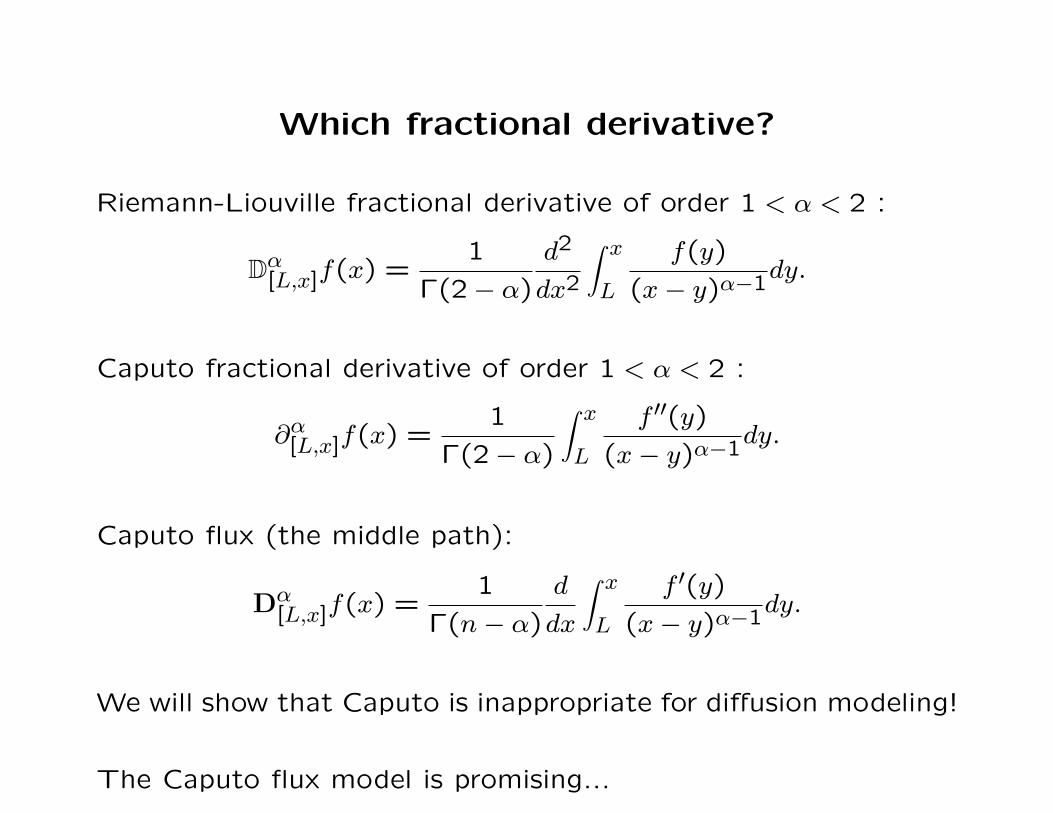
Which fractional derivative?

Riemann-Liouville fractional derivative of order 1 < α < 2 :

Dα[L,x]f(x) =

1

Γ(2− α)

d2

dx2

∫ x

L

f(y)

(x− y)α−1dy.

Caputo fractional derivative of order 1 < α < 2 :

∂α[L,x]f(x) =1

Γ(2− α)

∫ x

L

f ′′(y)

(x− y)α−1dy.

Caputo flux (the middle path):

Dα[L,x]f(x) =

1

Γ(n− α)

d

dx

∫ x

L

f ′(y)

(x− y)α−1dy.

We will show that Caputo is inappropriate for diffusion modeling!

The Caputo flux model is promising...

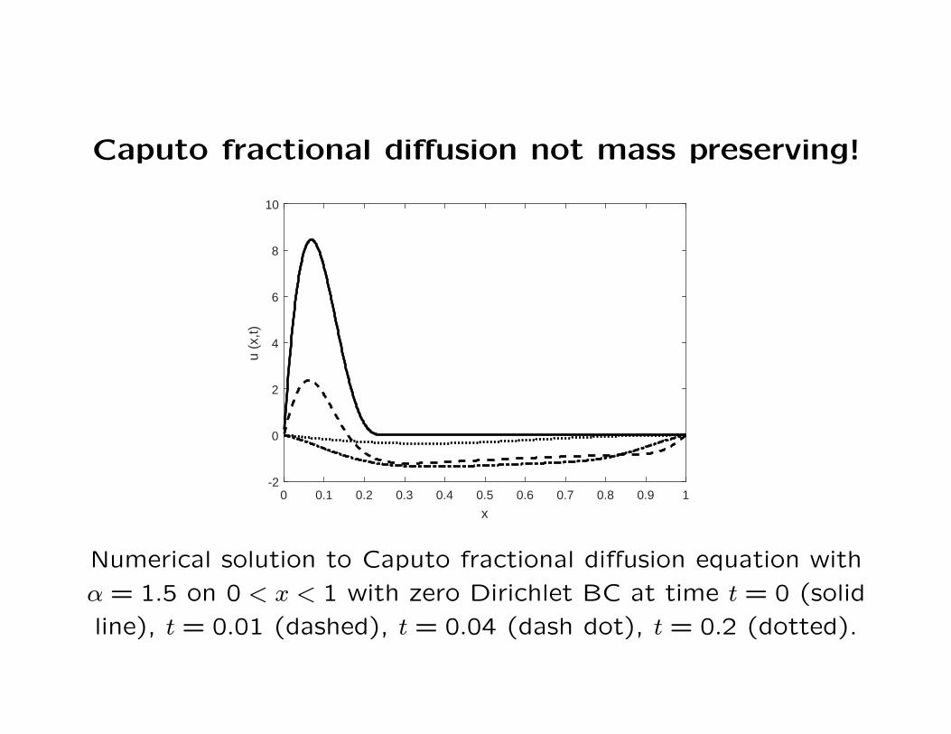
Caputo fractional diffusion not mass preserving!

0 0.1 0.2 0.3 0.4 0.5 0.6 0.7 0.8 0.9 1

x

-2

0

2

4

6

8

10

u (x

,t)

Numerical solution to Caputo fractional diffusion equation with

α = 1.5 on 0 < x < 1 with zero Dirichlet BC at time t = 0 (solid

line), t = 0.01 (dashed), t = 0.04 (dash dot), t = 0.2 (dotted).

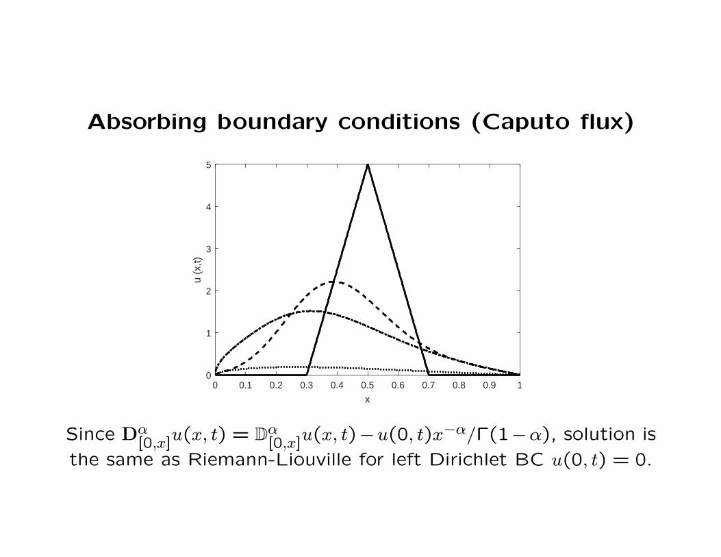
Absorbing boundary conditions (Caputo flux)

0 0.1 0.2 0.3 0.4 0.5 0.6 0.7 0.8 0.9 1

x

0

1

2

3

4

5

u (x

,t)

Since Dα[0,x]

u(x, t) = Dα[0,x]

u(x, t)−u(0, t)x−α/Γ(1−α), solution is

the same as Riemann-Liouville for left Dirichlet BC u(0, t) = 0.

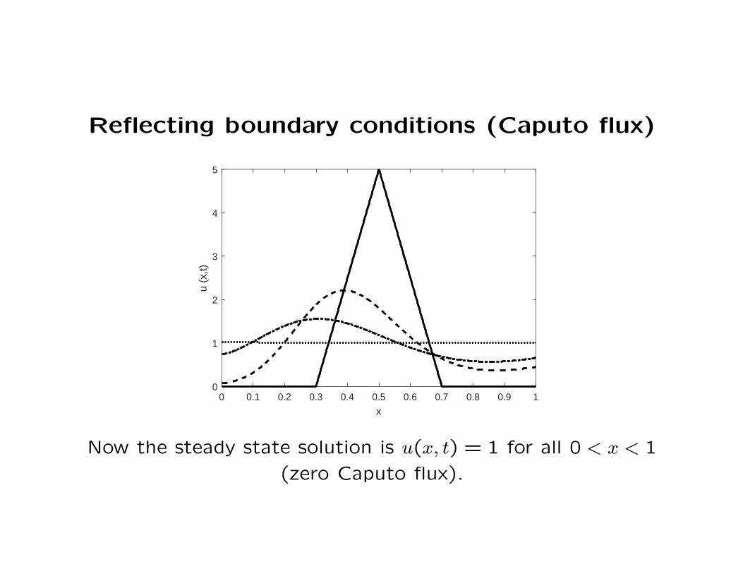
Reflecting boundary conditions (Caputo flux)

0 0.1 0.2 0.3 0.4 0.5 0.6 0.7 0.8 0.9 1

x

0

1

2

3

4

5

u (x

,t)

Now the steady state solution is u(x, t) = 1 for all 0 < x < 1

(zero Caputo flux).

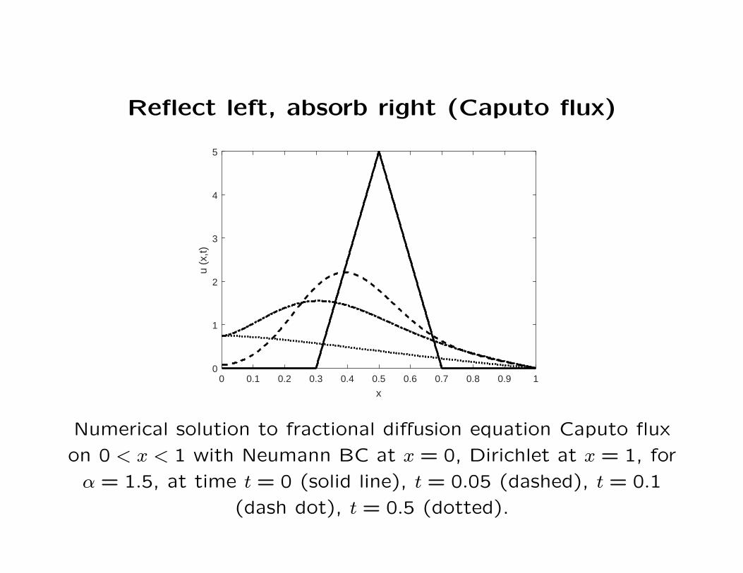
Reflect left, absorb right (Caputo flux)

0 0.1 0.2 0.3 0.4 0.5 0.6 0.7 0.8 0.9 1

x

0

1

2

3

4

5

u (x

,t)

Numerical solution to fractional diffusion equation Caputo flux

on 0 < x < 1 with Neumann BC at x = 0, Dirichlet at x = 1, for

α = 1.5, at time t = 0 (solid line), t = 0.05 (dashed), t = 0.1

(dash dot), t = 0.5 (dotted).

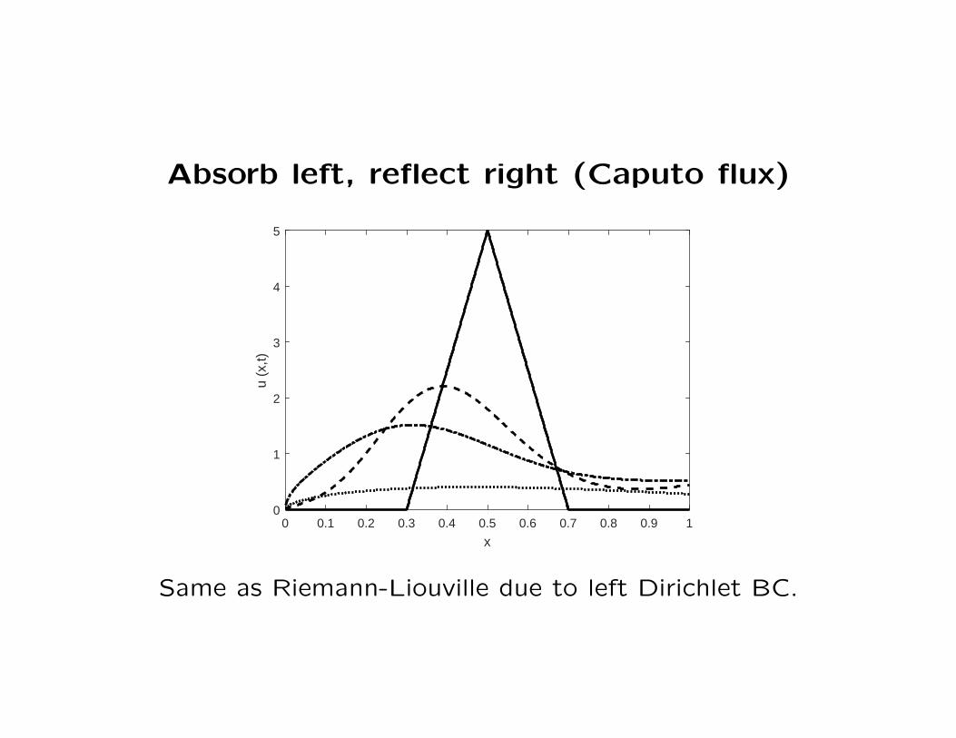
Absorb left, reflect right (Caputo flux)

0 0.1 0.2 0.3 0.4 0.5 0.6 0.7 0.8 0.9 1

x

0

1

2

3

4

5

u (x

,t)

Same as Riemann-Liouville due to left Dirichlet BC.

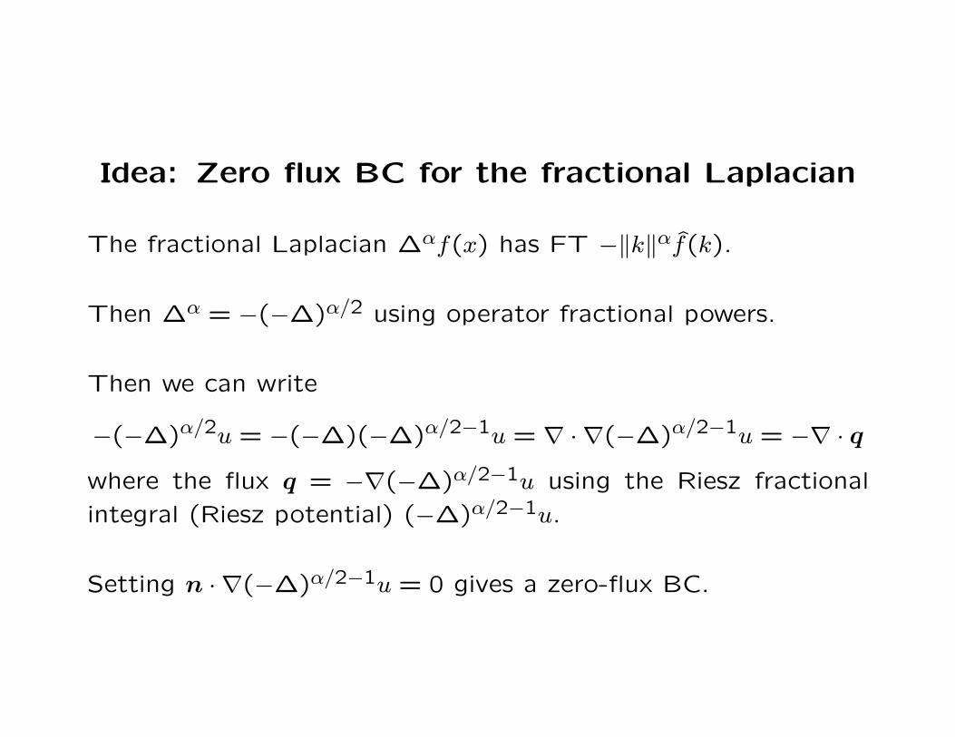
Idea: Zero flux BC for the fractional Laplacian

The fractional Laplacian ∆αf(x) has FT −‖k‖αf(k).

Then ∆α = −(−∆)α/2 using operator fractional powers.

Then we can write

−(−∆)α/2u = −(−∆)(−∆)α/2−1u = ∇ · ∇(−∆)α/2−1u = −∇ · q

where the flux q = −∇(−∆)α/2−1u using the Riesz fractional

integral (Riesz potential) (−∆)α/2−1u.

Setting n · ∇(−∆)α/2−1u = 0 gives a zero-flux BC.

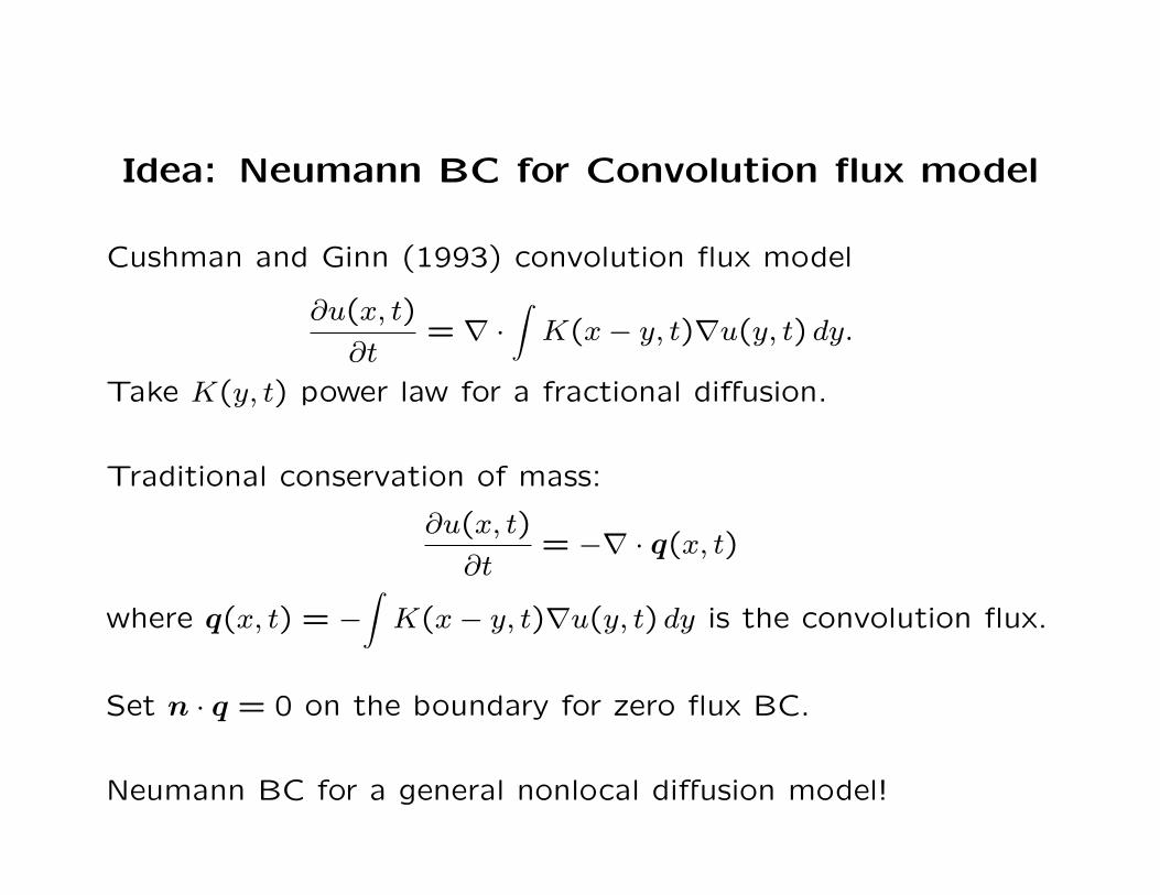
Idea: Neumann BC for Convolution flux model

Cushman and Ginn (1993) convolution flux model

∂u(x, t)

∂t= ∇ ·

∫

K(x− y, t)∇u(y, t) dy.

Take K(y, t) power law for a fractional diffusion.

Traditional conservation of mass:

∂u(x, t)

∂t= −∇ · q(x, t)

where q(x, t) = −∫

K(x− y, t)∇u(y, t) dy is the convolution flux.

Set n · q = 0 on the boundary for zero flux BC.

Neumann BC for a general nonlocal diffusion model!

Open problem: Numerical methods for Zolotarev dvt

Grunwald-Letnikov approximation for α 6= 1:

dαf(x)

dxα≈ h−α

∞∑

i=0

gαi f(x− (i− 1)h)

using the Grunwald weights

gαi = (−1)i(

αi

)

=−α(1− α) · · · (i− 1− α)

i!.

When α = 1 this is the first derivative!

For α = 1 we can write

Dα,1x f(x) =

2

π

∫ ∞

0

(

f(x− y)− f(x) + f ′(x) sin y)

y−2 dy

How can we approximate the Zolotarev derivative?

Products

Download at www.stt.msu.edu/users/mcubed

1. J.F. Kelly and M.M. Meerschaert, Space-time duality for the fractional advection dis-persion equation, Water Resources Research, Vol. 53 (2017), No. 4, pp. 3464–3475.

2. J.F. Kelly, D. Bolster, M.M. Meerschaert, J.D. Drummond, and A.I. Packman, FracFit:A Robust Parameter Estimation Tool for Fractional Calculus Models, Water ResourcesResearch, Vol. 53 (2017), No. 3, pp. 1763–2576.

3. M.S. Alrawashdeh, J,F. Kelly, M.M. Meerschaert, and H.-P. Scheffler, Applications ofInverse Tempered Stable Subordinators, Computers and Mathematics with Applications,Vol. 73 (2017), No. 6, pp. 892–905. DOI: 10.1016/j.camwa.2016.07.026. SpecialIssue on Time-fractional PDEs.

4. G. Didier, M.M. Meerschaert, and V. Pipiras, Domain and range symmetries of oper-ator fractional Brownian fields, Stochastic Processes and their Applications, Vol. 128(2018), No. 1, pp. 39–78.

5. G. Didier, M.M. Meerschaert, and V. Pipiras, Exponents of operator self-similar randomfields, Journal of Mathematical Analysis and Applications, Vol. 448 (2017), No. 2, pp.1450–1466.

6. B. Baeumer, M. Kovacs, and Harish Sankaranarayanan, Fractional partial differentialequations with boundary conditions. Journal of Differential Equations, Volume 264(2018), Issue 2, pp. 1377–1410. https://doi.org/10.1016/j.jde.2017.09.040

7. Anomalous Diffusion with Ballistic Scaling: A New Fractional Derivative, Journal ofComputational and Applied Mathematics, to appear the Special Issue on Modern frac-tional dynamic systems and applications (with James F. Kelly, Department of Statisticsand Probability, Michigan State University; and Cheng-Gang Li, Department of Math-ematics, Southwest Jiaotong University, Chengdu, China).

8. Boundary Conditions for Fractional Diffusion, revised for the Journal of Computationaland Applied Mathematics (with Boris Baeumer, Department of Mathematics and Statis-tics, University of Otago, Dunedin, New Zealand; Mihaly Kovacs, Department of Math-ematics, Chalmers University of Technology, Sweden; and Harish Sankaranarayanan,Department of Statistics and Probability, Michigan State University).

9. Space-time fractional Dirichlet problems, revised for Mathematische Nachrichten (withBoris Baeumer, Department of Mathematics and Statistics, University of Otago, Dunedin,New Zealand; and Tomasz Luks, Institut fur Mathematik, Universitat Paderborn, Ger-many).

10. A Unified Spectral Method for FPDEs with Two-sided Derivatives: A Fast Solver, re-vised for the Journal of Computational Physics (with Mohsen Zayernouri and MehdiSamiee, Department of Computational Mathematics, Science and Engineering, Michi-gan State University).

11. A Unified Spectral Method for FPDEs with Two-sided Derivatives: Stability and ErrorAnalysis, revised for the Journal of Computational Physics (with Mohsen Zayernouri andMehdi Samiee, Department of Computational Mathematics, Science and Engineering,Michigan State University).

12. Asymptotic behavior of semistable Levy exponents and applications to fractal path prop-erties, Journal of Theoretical Probability, to appear (with Peter Kern, MathematischesInstitut, Heinrich-Heine-Universitt Dsseldorf, Germany; and Yimin Xiao, Department ofStatistics and Probability, Michigan State University).

13. Relaxation patterns and semi-Markov dynamics, under review at Stochastic Processesand Their Applications (with Bruno Toaldo, Department of Statistical Sciences, SapienzaUniversity of Rome).

14. Parameter Estimation for Tempered Fractional Time Series, in revision (with FarzadSabzikar, Department of Statistics, Iowa State University; and A. Ian McLeod, Depart-ment of Statistical and Actuarial Sciences, University of Western Ontario).

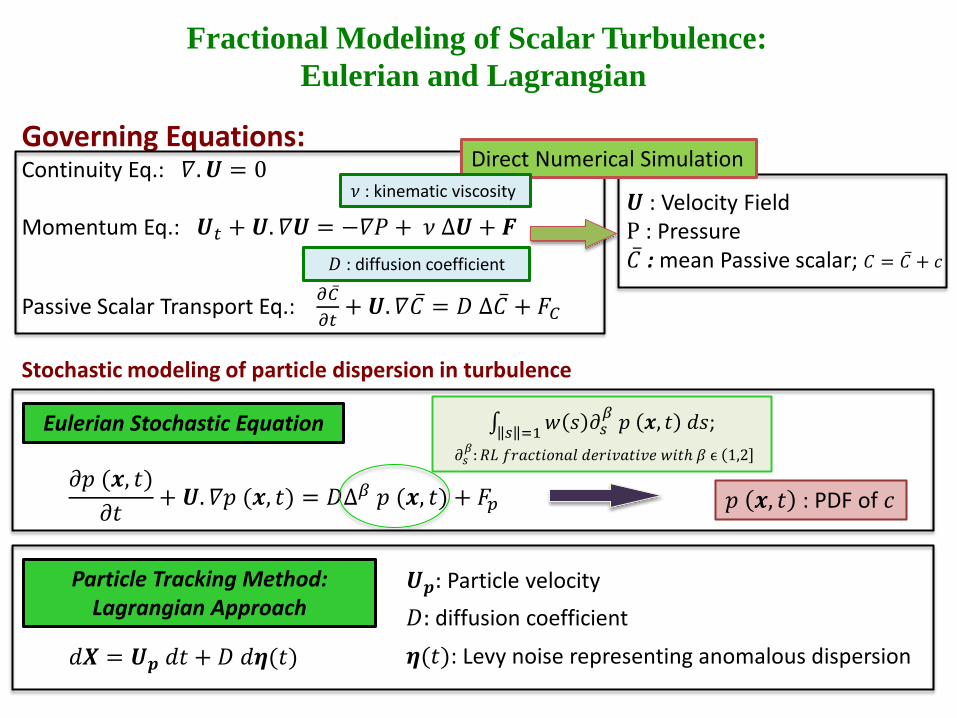
Governing Equations: Continuity Eq.: 𝛻.𝑼 = 0 Momentum Eq.: 𝑼𝑡 + 𝑼.𝛻𝑼 = −𝛻𝑃 + 𝜈 Δ𝑼 + 𝑭

Passive Scalar Transport Eq.: 𝜕��𝜕𝑡

+ 𝑼.𝛻�� = 𝐷 Δ�� + 𝐹𝐶 Stochastic modeling of particle dispersion in turbulence

Direct Numerical Simulation

Eulerian Stochastic Equation

Particle Tracking Method: Lagrangian Approach

𝜕𝑝 (𝒙, 𝑡)𝜕𝑡 + 𝑼.𝛻𝑝 (𝒙, 𝑡) = 𝐷∆𝛽 𝑝 (𝒙, 𝑡) + 𝐹𝑝

𝑑𝑿 = 𝑼𝒑 𝑑𝑡 + 𝐷 𝑑𝜼(𝑡) 𝜼(𝑡): Levy noise representing anomalous dispersion

∫ 𝑤 𝑠 𝜕𝑠𝛽 𝑝 𝒙, 𝑡 𝑑𝑠𝑠 =1 ;

𝜕𝑠𝛽:𝑅𝑅 𝑓𝑓𝑓𝑓𝑡𝑓𝑓𝑓𝑓𝑓 𝑑𝑑𝑓𝑓𝑑𝑓𝑡𝑓𝑑𝑑 𝑤𝑓𝑡𝑤 𝛽 ϵ 1,2

Fractional Modeling of Scalar Turbulence:

Eulerian and Lagrangian

𝑝 𝒙, 𝑡 : PDF of 𝑓

𝐷: diffusion coefficient 𝑼𝒑: Particle velocity

𝑼 : Velocity Field P : Pressure �� : mean Passive scalar; 𝐶 = 𝐶 + 𝑓

𝜈 : kinematic viscosity

𝐷 : diffusion coefficient

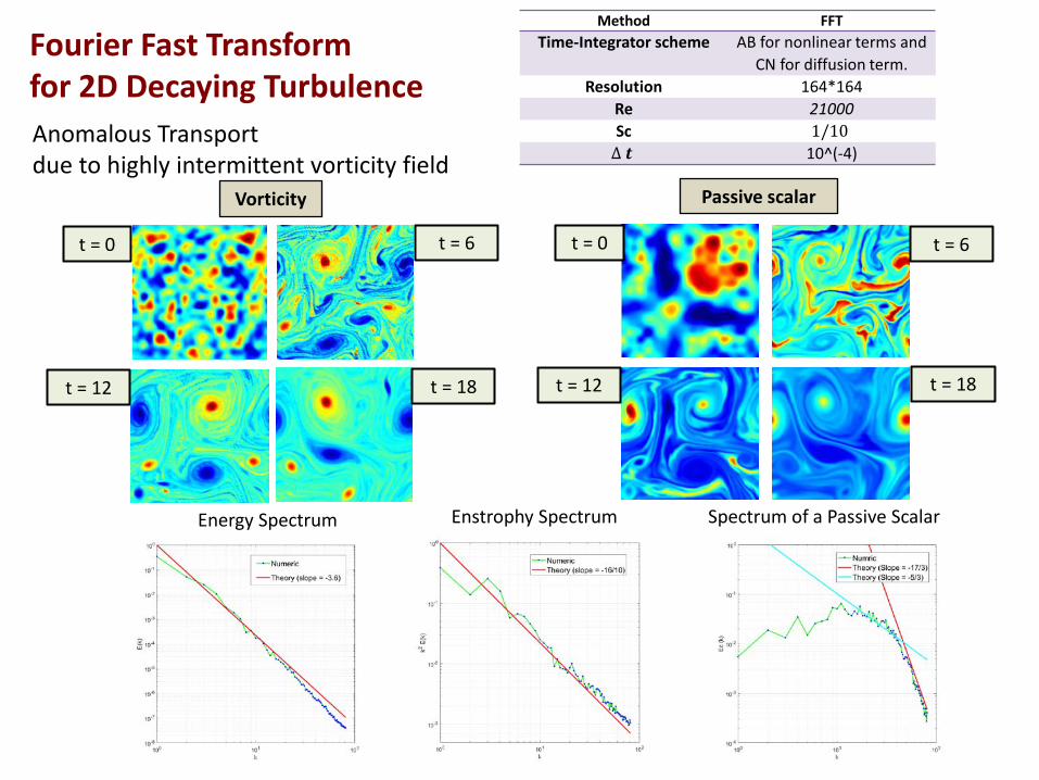
Method FFT Time-Integrator scheme AB for nonlinear terms and

CN for diffusion term. Resolution 164*164

Re 21000 Sc 1/10 ∆ 𝒕 10^(-4)

Anomalous Transport due to highly intermittent vorticity field

Fourier Fast Transform for 2D Decaying Turbulence

Vorticity Passive scalar

Energy Spectrum Enstrophy Spectrum Spectrum of a Passive Scalar

t = 0

t = 12

t = 6

t = 18

t = 0 t = 6

t = 12 t = 18

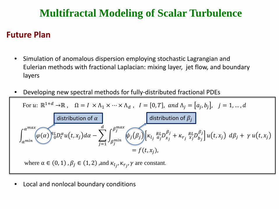
Multifractal Modeling of Scalar Turbulence Future Plan

• Simulation of anomalous dispersion employing stochastic Lagrangian and

Eulerian methods with fractional Laplacian: mixing layer, jet flow, and boundary layers

• Developing new spectral methods for fully-distributed fractional PDEs

• Local and nonlocal boundary conditions

� 𝜑 𝛼𝛼𝑚𝑚𝑚

𝛼𝑚𝑖𝑖𝐷𝑡𝛼0

𝑅𝑅 𝑢 𝑡, 𝑥𝑗 𝑑𝛼 −�� 𝜓𝑗 𝛽𝑗𝛽𝑗𝑚𝑚𝑚

𝛽𝑗𝑚𝑖𝑖

𝜅𝑙𝑗 𝐷𝑥𝑗𝛽𝑗

𝑎𝑗𝑅𝑅 + 𝜅𝑟𝑗 𝐷𝑏𝑗

𝛽𝑗𝑥𝑗𝑅𝑅 𝑢 𝑡, 𝑥𝑗 𝑑𝛽𝑗

𝑑

𝑗=1

+ 𝛾 𝑢 𝑡, 𝑥𝑗

= 𝑓(𝑡, 𝑥𝑗),

For 𝑢: ℝ1+𝑑 →ℝ , Ω = 𝐼 × Λ1 × ⋯× Λ𝑑 , 𝐼 = 0,𝑇 , 𝑓𝑓𝑑 Λ𝑗 = 𝑓𝑗 , 𝑏𝑗 , 𝑗 = 1, … ,𝑑

where α ∈ 0, 1 ,𝛽𝑗 ∈ 1, 2 ,and 𝜅𝑙𝑗 , 𝜅𝑟𝑗 , 𝛾 are constant.

distribution of 𝛼 distribution of 𝛽𝑗

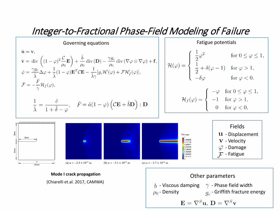
Integer-to-Fractional Phase-Field Modeling of Failure Governing equations Fatigue potentials

(Chiarelli et.al. 2017, CAMWA)

Mode I crack propagation

- Displacement - Velocity - Damage - Fatigue

Fields

Other parameters - Viscous damping - Density

- Phase field width - Griffith fracture energy

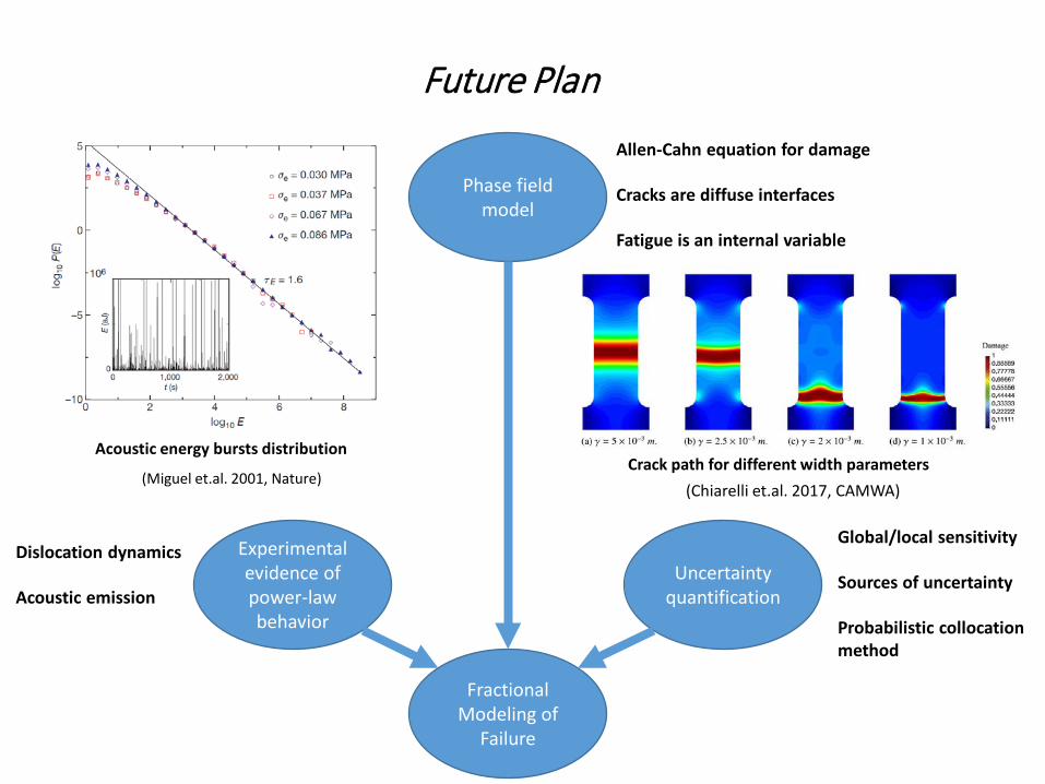
Future Plan

Uncertainty quantification

Phase field model

Fractional Modeling of

Failure

(Miguel et.al. 2001, Nature)

Experimental evidence of power-law behavior

(Chiarelli et.al. 2017, CAMWA)

Dislocation dynamics Acoustic emission

Global/local sensitivity Sources of uncertainty Probabilistic collocation method

Allen-Cahn equation for damage Cracks are diffuse interfaces Fatigue is an internal variable

Crack path for different width parameters Acoustic energy bursts distribution