A Search-Based Neoclassical Model of Capital Reallocation

FEDERAL RESERVE BANK OF ST. LOUISResearch Division

P.O. Box 442St. Louis, MO 63166

RESEARCH DIVISIONWorking Paper Series

Feng Dong,Pengfei Wang

andYi Wen

Working Paper 2018-017B https://doi.org/10.20955/wp.2018.017

August 2018

The views expressed are those of the individual authors and do not necessarily reflect official positions of the FederalReserve Bank of St. Louis, the Federal Reserve System, or the Board of Governors.

Federal Reserve Bank of St. Louis Working Papers are preliminary materials circulated to stimulate discussion andcritical comment. References in publications to Federal Reserve Bank of St. Louis Working Papers (other than anacknowledgment that the writer has had access to unpublished material) should be cleared with the author or authors.

A Search-Based Neoclassical Model of

Capital Reallocation∗

Feng Dong† Pengfei Wang‡ Yi Wen§

This Version: July, 2018

Abstract

As a form of investment, the importance of capital reallocation between firms has been increasingover time, with the purchase of used capital accounting for 25% to 40% of firms’ total investmentnowadays. Cross-firm reallocation of used capital also exhibits intriguing business-cycle properties,such as (i) the illiquidity of used capital is countercyclical (or the quantity of used capital reallocationacross firms is procyclical), (ii) the prices of used capital are procyclical and more so than those of newcapital goods, and (iii) the dispersion of firms’ TFP or MPK (or the benefit of capital reallocation)is countercyclical. We build a search-based neoclassical model to qualitatively and quantitativelyexplain these stylized facts. We show that search frictions in the capital market are essential for ourempirical success but not sufficient–financial frictions and endogenous movements in the distributionof firm-level TFP (or MPK) and interactions between used-capital investment and new investmentare also required to simultaneously explain these stylized facts, especially that prices of used capitalare more volatile than that of new investment and the dispersion of firm TFP is countercyclical.

Key Words: Capital Reallocation, Capital Search, Fragmented Markets, Endogenous Dispersionof firms’ TFP, Endogenous Total Factor Productivity, Business Cycles.

JEL Codes: E22, E32, E44, G11.

∗We have benefited from comments by Benoit Julien, Erica X.N. Li, Valerie Ramey, Zhiwei Xu, and in particular RandyWright, as well as participants at the Annual Conference on Money, Banking and Asset Markets at University of WisconsinMadison, Tsinghua Workshop in Macroeconomics, Shanghai University of Finance and Economics, and China InternationalConference in Finance. The views expressed here are only those of the individual authors and do not necessarily reflect theofficial positions of the Federal Reserve Bank of St. Louis, the Federal Reserve System, or the Board of Governors.

†Antai College of Economics and Management, Shanghai Jiao Tong University, Shanghai, China. Tel: (+86) 21-52301590.Email: fengdong@sjtu.edu.cn

‡Department of Economics, Hong Kong University of Science and Technology, Clear Water Bay, Hong Kong. Tel: (+852)2358 7612. Email: pfwang@ust.hk

§Federal Reserve Bank of St. Louis, P.O. Box 442, St. Louis, MO 63166; and School of Economics and Management,Tsinghua University, Beijing, China. Office: (314) 444-8559. Fax: (314) 444-8731. Email: yi.wen@stls.frb.org

1

1 Introduction

"In the process of creative destruction [...] many firms may have to perish that nevertheless

would be able to live on vigorously and usefully if they could weather a particular storm."

– J.A. Schumpeter, "Capitalism, Socialism, Democracy," Part II, Ch. VIII.

Merges, acquisitions and cross-firm trade in used capital have been an important form of firm invest-

ment and resource reallocation over the business cycle.1 For example, the existing empirical literature

(notably Ramey and Shapiro, 2001; Eisfeldt and Rampini, 2006; Cui, 2014; Lanteri, 2015; Kehrig, 2015;

Kurmann, and Pestroky-Nadeau, 2007; among others) documents that the purchase of used capital alone

(not including acquisitions and merges) accounts for more than 25% of firm investment, suggesting the

importance and significance of capital reallocation across firms in the economy. Moreover, this empirical

literature (most notably Eisfeldt and Rampini, 2006) identifies several firm-level business-cycle facts on

capital reallocation that have attracted a growing amount of theoretical studies, such as:

1. the dispersion of firms’ total factor productivity (TFP) or marginal product of capital (MPK) is

counter-cyclical, suggesting that the benefit of cross-firm capital reallocation is high in recessions

and low in booms;2

2. however, firm investment in used capital is strongly procyclical and as volatile as gross domestic

product (GDP);

3. the prices of used capital are strongly procyclical.

Table 1 quantifies the three stylized facts documented by Eisfeldt and Rampini (2006). At the business-

cycle frequencies (under HP filter), The correlation of dispersion of firms’ TFP and output (real GDP) is

strongly negative and significant, with a point estimate of -0.465. For capital reallocation the correlation

is strongly positive and significant, with a point estimate of 0.637. For acquisitions the correlation is

0.675, for PPE (sales of property, plant and equipment) it is 0.329, for prices of used capital it is 0.565,

all are statistically significant.

Table 1. Reallocation of Capital∗

TFP dispersion reallocation acquisitions sales of PPE PricesCorrelation with output -0.465 (0.194) 0.637 (0.112) 0.675 (0.122) 0.329 (0.173) 0.565 (0.08)∗Numbers in parentheses are standard errors. Data source: Eisfeldt and Rampini (2006).

1See Chang (2011) among others on labor reallocation with frictions.2Following Eisfeldt and Rampini (2006), Kehrig (2015) uses US census manufacturing data to document the counter-

cyclicality of the dispersion of firm TFP. In addition, if the benefit of reallocation is measured by the dispersion of firm-levelTobin’s q, it is also weakly countercyclical, suggesting higher benefit of acquiring used capital in recessions than in booms(see Eisfeldt and Rampini, 2006).

2

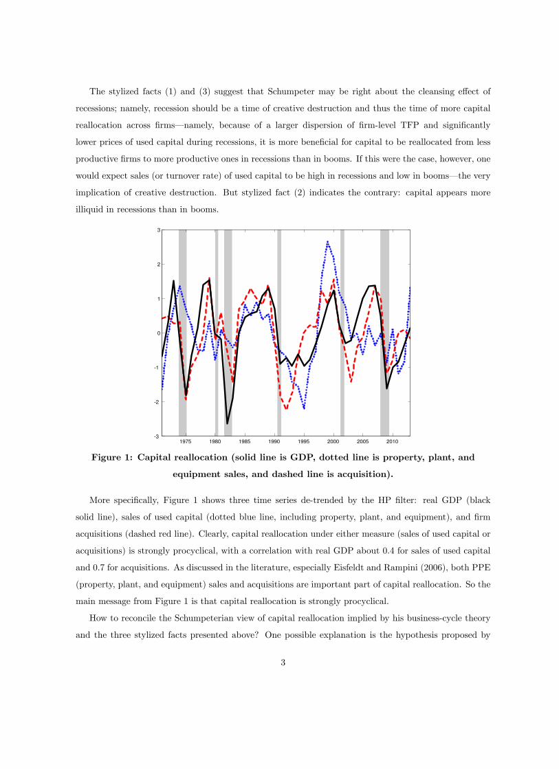
The stylized facts (1) and (3) suggest that Schumpeter may be right about the cleansing effect of

recessions; namely, recession should be a time of creative destruction and thus the time of more capital

reallocation across firms–namely, because of a larger dispersion of firm-level TFP and significantly

lower prices of used capital during recessions, it is more beneficial for capital to be reallocated from less

productive firms to more productive ones in recessions than in booms. If this were the case, however, one

would expect sales (or turnover rate) of used capital to be high in recessions and low in booms–the very

implication of creative destruction. But stylized fact (2) indicates the contrary: capital appears more

illiquid in recessions than in booms.

1975 1980 1985 1990 1995 2000 2005 2010

-3

-2

-1

0

1

2

3

Figure 1: Capital reallocation (solid line is GDP, dotted line is property, plant, and

equipment sales, and dashed line is acquisition).

More specifically, Figure 1 shows three time series de-trended by the HP filter: real GDP (black

solid line), sales of used capital (dotted blue line, including property, plant, and equipment), and firm

acquisitions (dashed red line). Clearly, capital reallocation under either measure (sales of used capital or

acquisitions) is strongly procyclical, with a correlation with real GDP about 0.4 for sales of used capital

and 0.7 for acquisitions. As discussed in the literature, especially Eisfeldt and Rampini (2006), both PPE

(property, plant, and equipment) sales and acquisitions are important part of capital reallocation. So the

main message from Figure 1 is that capital reallocation is strongly procyclical.

How to reconcile the Schumpeterian view of capital reallocation implied by his business-cycle theory

and the three stylized facts presented above? One possible explanation is the hypothesis proposed by

3

Eisfeldt and Rampini (2006) that the cost of reallocating capital is strongly countercyclical so that capital

appears more liquid in booms than in recessions. This hypothesis, however, does not reveal the underling

mechanism of the countercyclical costs of capital reallocation. Why is it more costly to sell/purchase

used capital in recessions when firms are stuck with excess capacity and desperately need more cash to

repay their debts?

Another possible explanation is the idea of financial friction proposed by Kiyotaki and Moore (2012)

that asset resaleability is low in recessions and high in booms, resulting in procyclical turnover rate of

used capital. Indeed, the probability of selling used capital is procyclical (Eisfeldt and Rampini, 2016),

suggesting that the resaleability of capital is procyclical (Kiyotaki and Moore, 2012). But this theory

also fails to provide the underling mechanism of countercyclical resaleability and it also implies that the

price of used capital is high in recessions when less capital are available for sale, but low in booms when

more capital are available for sale–which contradicts stylized fact (3) above.

Our explanation detailed in this paper is search and matching in the used capital market. Since

search efforts are endogenously procyclical, the measured "costs" and "resaleability" of capital appear

to be countercyclical. Thus, un-utilized capital (capacity) is like unemployed labor, both have lower

market values in recessions and higher market values in booms. Allocative efficiency through search and

matching implies that capital is less misallocated in booms than in recessions, leading to a countercyclical

dispersion of firm-level TFP or Tobin’s q.

But we also show that search frictions are not enough albeit essential in explaining the data. Search

frictions can generate costs of capital reallocation in the steady state, but not their aggregate move-

ments without aggregate shocks. Yet different types of aggregate shocks (such as aggregate TFP shocks,

preference shocks, or financial shocks) can all generate movements in aggregate output, but they may

have different implications for the movements in the volume and prices of capital and the comovements

between aggregate output and the dispersion of firms’ TFP.

In this paper, we embed search frictions in the used capital market into a standard neoclassical model

to qualitatively and quantitatively rationalize the stylized facts. The neoclassical framework imposes

strong discipline on our analysis not only because we can introduce different types of aggregate shocks to

generate equilibrium fluctuations, but also because the decision to purchase or sell used capital is only

part of firms’ investment problems and thus must be studied together with decisions for new investment

and dynamic capital accumulation over a long horizon, all of which may be dictated by common macro-

economic forces such as financial frictions. If under certain aggregate shocks the demand for production

factors (labor or capital) are high in booms, firms not only invest more in new capital but would also

search harder for used capital, so both the turnover rate of used capital and new investment as well

4

as their prices would be procyclical. However, the procyclical capital reallocation across firms does not

necessarily imply that the benefit of capital reallocation (or illiquidity) is countercyclical, especially when

firms’ investment is financially constrained.

In addition to the three stylized facts listed above, there also exist other empirical regularities in the

firm-level data to test our model, such as (i) the prices of used capital is more procyclical and twice as

volatile as that of new capital goods (Lanteri, 2015), and (ii) the dispersion of firms’ gross investment rate

is procyclical despite the fact that the dispersion of firms’ TFP is countercyclical (Eisfeldt and Rampini,

2006).

We study the implications of three types of aggregate shocks: aggregate TFP shocks, financial shocks

to firms’ borrowing constraints, and shocks to matching efficiency. We find that all the three shocks can

generate procyclical movements in the volume and prices of used capital, but only under the "right" type

of aggregate shocks can search frictions simultaneously explain all of the stylized facts presented above,

especially the countercyclical dispersion of firm-level TFP.

The main intuition for the different degree of successes of different aggregate shocks is that search

friction in general leads to equilibrium capital "unemployment", i.e., the proportion/probability of selling

out un-utilized capital is below 100% at any point in time.3 Equilibrium capital unemployment, however,

may imply that the prices of used capital are less volatile than that of new capital goods, contradicting

with the data. This is especially the case if search frictions in the capital markets are endogenously coun-

tercyclical due to time-varying search efforts. In other words, higher aggregate demand for capital (both

used and new) during a boom leads to higher prices of capital in general, but the prices of used capital

rise significantly more than those of new capital only if the demand for used capital is proportionately

stronger than that of new capital in a boom for any given level of search frictions.

Also, the procyclical capital reallocation implies that resources are less misallocated during booms than

in recessions, which may or may not necessarily imply that the dispersion of firms’ TFP is countercyclical

unless the distribution of firms TFP is endogenously affected by both aggregate shocks and search frictions

in certain ways. Therefore, a fully-fledged DSGE model is required to sort out these complicated issues

even if we believe that search frictions are important in explaining the stylized empirical facts about

capital reallocation.

Hence, we build a model in which not only firms’ investment in used capital and new capital interact

with each other, but search frictions in the capital market also interact with credit frictions in the financial

market in important ways such that the distribution of firms’ TFP can endogenously respond to different

types of aggregate shocks.

3Capital "unemployment" is the same thing as excess capacity or capital hoarding during recessions.

5

Our work complements the existing literature on capital reallocation. Eisfeldt and Rampini (2006)

show that if the costs of reallocating capital are countercyclical, then capital reallocation would be

procyclical. However, they do not explain why prices of used capital are more procyclical than those of

new capital goods and why the dispersion of firms TFP is countercyclical. Lanteri (2015) also studies

the business-cycle dynamics of secondary markets for physical capital and tries to explain why the prices

of used capital are twice as volatile as those of new capital over the business cycle. However, Lanteri

(2015) does not use search frictions to explain this fact and he does not address the other stylized facts

of capital reallocations.

We are not the first to use search frictions in the capital markets to explain the stylized facts on

capital reallocations.4 First, Kurmann, and Pestroky-Nadeau (2007) build a dynamic model with search

frictions for capital allocation from households to representative firms, and then use the model to inves-

tigate implications of search frictions for the business cycle. Ottonello (2015) studies the issue of capital

unemployment as well, but he mainly addresses the effect of search frictions for the slump of new invest-

ment after the 2007 financial crisis (as it takes time to transform resources into investment goods under

search frictions). Cao and Shi (2017) build a simple model to address some of the stylized facts presented

above. However, their model is unable to generate countercyclical dispersion of firms’ productivity or

TFP, thus contradicting the first stylized fact presented in the very beginning of the paper. Also, their

model is not a genuine DSGE model with capital accumulation, so their model is unable (i) to reveal the

different implications of different aggregate shocks on capital reallocation under search, (ii) to address

the interactions between used capital investment and new investment, and (iii) to generate endogenous

movements in the distribution of firms’ TFP. frictions.5 Wright, Xiao and Zhu (2017) develop a model of

capital reallocation based on Lagos and Wright (2005) model where firms trade used capital in frictional

markets with either ex ante or ex post firm heterogeneity under different market microstructures. Finally,

Kurmann and Rabinovich (2017) develop a purely theoretical model of capital reallocation to study the

efficiency implications of bargaining in frictional capital markets for capital reallocation.

The rest of the paper proceeds as follows. Section 2 builds the model. Section 3 characterizes the

equilibrium properties of the model. Section 4 conducts a series of quantitative analysis after calibrating

to the US economy. Section 5 lists several model extensions. Section 6 concludes. Data description and

4 In addition to capital search, there is a burgeoning literature on finance search, i.e. asset trading in over-the-counter(OTC) markets. See Duffie, Garleanu and Pedersen (2005), Lagos and Rocheteau (2009), Hugonnier, Lester and Weill (2014),Afonso and Lagos (2015), Atkeson, Eisfeldt and Weill (2015), Trejos and Wright (2016), Lester, Shourideh, Venkateswaranand Zetlin-Jones (2017) and Zhang (2017) among others for the theoretical analysis of OTC markets. Besides, see Wasmerand Weil (2004), Cui and Radde (2014), Dong, Wang and Wen (2016), and Petrosky-Nadeau and Wasmer (2013, 2015) forcredit search. Also see Silveira and Wright (2010) and Chiu, Meh and Wright (2017) on search for ideas.

5More specifically, their model is more stylized with two types of firms and a firm can either have 1 unit or 0 unit ofcapital, as in the first-generation of money-search models.

6

proofs are put in the Appendix.

2 Model

2.1 Environment

Time is discrete with t = 0, 1, 2, ...,∞. There are three types of agents: (i) a representative household,(ii) a unit measure of heterogeneous firms, and (iii) a unit measure of capital dealers (intermediaries) in

the used capital markets.

The representative household is the owner of firms and intermediaries, and makes decisions on con-

sumption, labor supply to firms, and holdings of firm equities.

Firms receive both aggregate and idiosyncratic productivity shocks in the beginning of each period.

After observing these shocks, each firm decides whether to purchase or sell used capital in the secondary

capital markets. Firms opting to purchase used capital need to search and meet capital dealers in the

buyers’ market, while firms opting to sell used capital need to search and meet capital dealers in the

sells’ market. Capital dealers can freely move across the two types of capital markets, but firms cannot.

Capital reallocation across firms is realized only through search and bilateral trading with capital dealers

in decentralized capital markets. The terms of trade is determined by Nash bargaining.

The matching technology in the sellers’ buyers’ markets are given, respectively, by MS(xS , S

)and

MB(xB , B

), where xS and xB denote, respectively, the measure of dealers in the sellers’ market and the

buyers’ market, and S and B the measure of firms selling capital (capital sellers) and firms buying capital

(capital buyers). Both matching functions are constant returns to scale. The matching probabilities for

firms(pS , pB

)and dealers

(qS , qB

)are determined, respectively, by pS ≡ MS(xS ,S)

S , qS ≡ MS(xS ,S)xS

,

pB ≡ MB(xB ,B)B , and qB ≡ MB(xB ,B)

xB; the market tightness in each market is θS ≡ S/xS and θB ≡ B/xB .

To focus on the implication of search frictions for capital reallocation, we rule out any information

frictions. Therefore, firms’ productivity and their outside options are public knowledge, at least to the

dealers the firms are matched with.

After trading in the decentralized capital markets, each firm makes decisions on production (employ-

ment), investment for new capital, and dividends distributed to shareholders.

Figure 4 shows schematically the two decentralized capital markets for seller-firms and buyer-firms,

where{QS (z) , QB (z) , QD

}denote respectively the terms of trade for the seller-firms, buyer-firms, and

the dealers. Note that the dealers face the same terms of trade QD in both the sellers’ market and the

buyers’ market under free arbitrage across these markets.

7

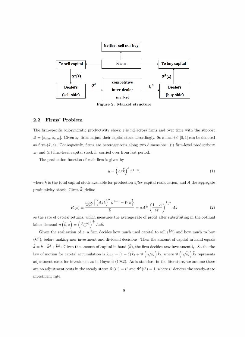
Figure 2. Market structure

2.2 Firms’ Problem

The firm-specific idiosyncratic productivity shock z is iid across firms and over time with the support

Z = [zmin, zmax]. Given zt, firms adjust their capital stock accordingly. So a firm i ∈ [0, 1] can be denotedas firm-(k, z). Consequently, firms are heterogeneous along two dimensions: (i) firm-level productivity

zt, and (ii) firm-level capital stock kt carried over from last period.

The production function of each firm is given by

y =(Azk̃

)αn1−α, (1)

where k̃ is the total capital stock available for production after capital reallocation, and A the aggregate

productivity shock. Given k̃, define

R (z) ≡maxn≥0

{(Azk̃

)αn1−α −Wn

}

k̃= αA

1α

(1− αW

) 1−αα

Az (2)

as the rate of capital returns, which measures the average rate of profit after substituting in the optimal

labor demand n(k̃, z)=((1−α)W

) 1α

Azk̃.

Given the realization of z, a firm decides how much used capital to sell (k̃S) and how much to buy

(k̃B), before making new investment and dividend decisions. Then the amount of capital in hand equals

k̃ = k− k̃S+ k̃B . Given the amount of capital in hand (k̃), the firm decides new investment it. So the thelaw of motion for capital accumulation is kt+1 = (1− δ) k̃t +Ψ

(it/k̃t

)k̃t, where Ψ

(it/k̃t

)k̃t represents

adjustment costs for investment as in Hayashi (1982). As is standard in the literature, we assume there

are no adjustment costs in the steady state: Ψ(i∗) = i∗ and Ψ′ (i∗) = 1, where i∗ denotes the steady-state

investment rate.

8

The resource constraint for new investment is given by it = Rt (zt) k̃t + k̃St QSt (zt)− k̃Bt Q

Bt (zt)− dt,

where the first term is profit from production, the second term is the value added from capital sales, the

third term is the cost of purchasing used capital, and dt is dividend.

Due to search frictions in the used capital markets, only k̃S (kt, zt) ≡ pSt kSt units of capital are

traded between a dealer and a firm-(kt, zt) that intends to sell kSt units of capital. Similarly, only

k̃B (kt, zt) ≡ pBt kBt units of capital are traded between a dealer and a firm-(kt, zt) that intends to buy k

Bt

units of capital. The intended capital-to-sell and intended capital-to-buy satisfy the following constraints:

kS ≤ k and kB ≤ µpSt k. The former denotes a feasibility condition and the latter a borrowing constraint

faced by capital-buyers, where µ captures financial frictions a la Kiyotaki and Moore (1997), Bernanke,

Gertler and Gilchrist (1999) and Jermann and Quadrini (2012). Note that the borrowing constraint is

endogenous since the collateral depends on how liquid the asset is (i.e., the probability of matching pS).

Since we assume that dealers can be in one market only (at any moment) but can nonetheless freely

enter either market, namely, dealers in the capital sellers’ market can purchase used capital from capital

sellers and sell the used capital to other dealers in the capital buyers’ market through inter-dealer trading,

they face the same terms of trade QD in both the sellers’ market and the buyers’ market.6

To summarize, the optimization problem of firm-(k, z) in time t is to choose{kSt , k

Bt , it, dt

}to maxi-

mize the present value of future dividends. The value of firm-(kt, zt) is then given by

Vt (kt, zt) = maxkSt ,k

Bt ,it,dt

{dt + Et

βΛt+1Λt

∫Vt+1 (kt+1, zt+1) dF (zt+1)

}, (3)

subject to

k̃t = kt − pSt kSt + pBt kBt , (4)

dt + it = Rt (zt) k̃t + pSt k

St Q

St (zt)− pBt kBt QBt (zt) , (5)

kt+1 = (1− δ) k̃t +Ψ(it/k̃t

)k̃t, (6)

kSt ∈ [0, kt] , (7)

kBt ∈[0, µpSt kt

]. (8)

2.3 Household

A representative household solves

maxCt,Nt,st+1

E0

∞∑

t=0

βt

[log (Ct)− ψ

N1+γt

1 + γ

], (9)

6This assumption simplifies our analysis and is harmless. We later show that our results hold when the same dealer canpurchase capital and sell it to firms or firms simply search for each other in bilateral meetings (see the remark in section3.2).

9

subject to

Ct +

∫

i∈[0,1]

sit+1(V it − dit

)di =

∫

i∈[0,1]

sitVit di+Π

dt +WtNt, (10)

where β denotes the discount factor, Ch consumption, Nt labor supply,(V it , s

it

)the value of firm-i and the

associated share holdings by the household. The household receives total profits Πdt from intermediaries

and labor income WtNt from work. Denote Λt as the Lagrangian multiplier of the household’s budget

constraint, the first order conditions (FOCs) on consumption (Ct), labor supply (Nt) and share holdings(sit+1

)i∈[0,1]

are given by

Λt =1

Ct, (11)

ΛtWt = ψNγt , (12)

V jt = djt + EtβΛt+1Λt

V jt+1. (13)

where βΛt+1/Λt denotes the pricing kernel.

2.4 Equilibrium

An equilibrium consists of a series of prices and quantities such that (i) given prices, the household, firms

and dealers maximize their own objective functions; and (ii) all markets clear.

3 Characterization of Capital Market Equilibrium

3.1 Firms

As is standard in the adjustment cost literature, given k̃t, the FOC for new investment it implies

1 = Ψ′i

(it/k̃t

)k̃tEt

βΛt+1Λt

∂Vt+1 (kt+1, zt+1)

∂kt+1(14)

≡ Ψ′i/k̃

(it/k̃t

)Qt,

where Qt denotes Tobin’s Q–the marginal value of one unit of new capital:

Qt ≡ E[(

βΛt+1Λt

)φt+1 (zt+1)

]. (15)

In turn, equation (14) implies that investment can be expressed as

it = ω (Qt) k̃t, (16)

where ω (Qt) ≡ Ψ′−1 (Qt). Since Ψ(ι) is assumed to be strictly concave, ω (Qt) is strictly increasing inTobin’s Q.

10

We guess and will verify later that firm’s value function is linear in capital kt:

Vt (kt, zt) = φt (zt) kt. (17)

Substituting equations (17) and (16) into firm-(k, z)’s optimization problem (3) yields

φt (zt) kt = max{kSt , kBt }

{(mt +Qt (1− δ)) kt +[QSt (zt)−mt

]pSt k

St +

[mt −QBt (zt)

]pBt k

Bt }, (18)

where mt ≡ [Rt (zt) + Γ (Qt)] denotes the marginal-value product of capital; so the term in the first

square brackets on the right-hand side is the gain from trade by selling one unit of used capital, and the

term in the second square brackets is the gain from trade by purchasing one unit of used capital. Notice

that the marginal-value product of capital has two terms: the marginal product R (z) and an additional

term Γ (Q) defined by

Γ (Qt) ≡ Qt (1− δ) +QtΨ(ω (Qt))− ω (Qt) . (19)

This additional term reflects the option value of capital arising from adjustment costs of investment–

since installing new capital through investment is costly, having one additional unit of capital in hand

avoids the adjustment costs with the gain of Γ (Q). When the adjustment costs vanish, we have Qt = 1

and Γ (Qt) = QtΨ(ω (Qt))− ω (Qt) = Qti

k̃− i

k̃= 0.

3.2 Terms of Trade

Proposition 1 A firm-(z, k) opts to be a capital seller if z ≤ z∗ and a capital buyer if z > z∗. The terms

of trade between the capital seller and a dealer is given by

QSt (z) = (1− η)QDt + η (Rt (zt) + Γ (Qt)) , if z ≤ z∗, (20)

and the terms of trade between the capital buyer and a dealer is given by

QBt (z) = (1− η)QDt + η (Rt (zt) + Γ (Qt)) , if z > z∗, (21)

where z∗ is the cutoff productivity at which we have

QS

t (z∗t ) = Q

B

t (z∗t ) = Rt (z

∗t ) + Γ (Qt) = Q

D. (22)

Proof: See Appendix I.

The terms of trade indicate that the gains from trade are split between the firm and the dealer,

depending on their respective bargaining power η ∈ [0, 1]. If the dealer has all the bargaining power,η = 1, then the terms of trade QS = R (z) + Γ (Q) for z ≤ z∗ and QB = R (z) + Γ (Q) for z > z∗,

so firms earn zero profits from trade. Since the marginal product of capital R (z) is increasing in z, we

11

have QS ≤ QD ≤ QB . It is worth noting that{QSt , Q

B}are independent of kt and are both increasing

functions of z.

Remark 1 For tractability, we have assumed that firms do not directly trade with each other for capital

reallocation. Alternatively, we can let firms directly contact each other in bilateral trading between high-

productivity firm i ∈ B and low-productivity firm j ∈ S. We know that R (i) ≥ R (j) holds for i ∈ B andj ∈ S. Since z shock is iid over time and across firm, the terms of trade (price of capital), Q (i, j), isdetermined by Nash bargaining as below,

argmaxx∈[R(i),R(j)]

{(R (i)−Q (i, j))η (Q (i, j)−R (j))1−η

}, (23)

which delivers

Q (i, j) = (1− η)R (i) + ηR (j) . (24)

where η ∈ (0, 1) denotes the bargaining power of the buyer. Then the expected prices facing i ∈ B andj ∈ S, are given respectively by

Q (i) = E (P (i, j) |j ∈ S) , (25)

Q (j) = E (P (i, j) |i ∈ B) . (26)

We can then verify that the linear structure of the model is still well preserved, but the algebra is more

involved.

3.3 Value of the Firm

Now we characterize the value function φt (·). Substituting equations (20) and (21) into (18) yields

individual firm’s Tobin Q, i.e., the shadow value of a firm with each additional unit of capital with

productivity zt at the beginning of time t, is

φt (zt) = maxkSt ∈[0,kt],k

Bt ∈[0,µtkt]

{(Rt (zt) + Γ (Qt)) kt

+(1− η) (Rt (z∗t )−Rt (zt)) pSt kSt + (1− η) (Rt (zt)−Rt (z∗t )) pBt kBt }. (27)

This immediately generates the policy functions of individual firm’s capital reallocation as below:

Lemma 1 The individual firm’s supply and demand of used capital is given by

kSt (kt, zt) =

{kt, if zt ≤ z∗t0, otherwise

, kBt (kt, zt) =

{0, if zt ≤ z∗tµtkt, otherwise

, (28)

and the level of firm’s capital stock after reallocation is given by

k̃t (kt, zt) = kt − pSt kSt + pBt kBt ={(1− pSt

)kt, if zt ≤ z∗t(

1 + µtpBt

)kt, otherwise

. (29)

12

As indicated in Lemma 1, the demand and supply of used capital is characterized by a cut-off strategy.

Firms with low productivity opt to sell their used capital while firms with high productivity opt to

purchase used capital. Due to the linear structure shown in equation (27), both seller- and buyer-firms

will choose a corner solution, i.e., they sell and buy as much as they can. However, due to search frictions

in capital reallocation, only pSt and pBt fraction of firms’ intended capital sales (purchases) are realized.

Substituting equation (28) into equation (27) simplifies individual firm’s Tobin Q as

φt (zt) = Rt (zt) + Γ (Qt) (30)

+(1− η) pSt (Rt (z∗t )−Rt (zt))1{zt≤z∗t } + µt (1− η) pBt (Rt (zt)−Rt (z∗t ))1{zt>z∗t }︸ ︷︷ ︸

real-option value from capital reallocation

.

The first line on the RHS of equation (30) is the marginal-value product of capital, the second line denotes

the additional benefit from capital reallocation. Note that φt (zt) is independent of kt, and therefore the

conjecture in equation (17) is verified.

Combining equations (15) and (30) yields the expected (aggregate) Tobin Q as

Qt = E

[(βΛt+1Λt

)(∫Rt+1 (z) dF (z) + Γ (Qt+1)

)]

︸ ︷︷ ︸neoclassical value

+E

[(βΛt+1Λt

)(1− η) pSt+1

∫ z∗t+1

zmin

(Rt+1

(z∗t+1

)−Rt+1 (z)

)dF (z)

]

︸ ︷︷ ︸option value from selling capital through search

+E

[(βΛt+1Λt

)µt+1 (1− η) pBt+1

∫ zmax

z∗t+1

(Rt+1 (z)−Rt+1

(z∗t+1

))dF (z)

]

︸ ︷︷ ︸option value from purchasing capital through search

, (31)

Given Tobin’s Qt, the new investment and gross investment are given respectively by

it (kt, zt) = ω (Qt) k̃t (kt, zt) , (32)

igt (kt, zt) = k̃t (kt, zt)− kt + it (kt, zt) . (33)

3.4 Inter-Dealer Market

The cut-off strategy of buying and selling capital implies that the number of sellers is given by St ={z| z ∈ [zmin, z∗t ] , ∀ kt} and the number of buyers is given by Bt = {(kt, zt) | z ∈ [z∗t , zmax] , ∀ kt}. Thenthe measure of seller-firms and that of buyer-firms is given respectively by

St (z∗t ) = F (z∗t ) , Bt (z

∗t ) = 1− F (z∗t ) . (34)

13

In turn, the total supply and demand of used capital in the markets are given respectively by

KSt ≡

∫ ∫

St

kSt dF (z) dG (k) = KtSt, (35)

KBt ≡

∫ ∫

Bt

kBt dF (z) dG (k) = µtKtBt. (36)

Following Lagos and Rocheteau (2009) and Zhang (2017), we assume there exists a competitive inter-

dealer market in which dealers’ total demand for capital equals dealers’ total supply of capital, i.e.,

KSt p

St = KB

t pBt . Then we have

StpSt = µtBtp

Bt , (37)

or equivalently,

MS(xSt , St

)= µtMB

t

(xBt , Bt

), (38)

where the LHS and RHS of the above equation denote, respectively, the total matched amount of capital

in the capital-sellers’ market and capital-buyers’ market. Clearly, the financial friction µt affects the

prices of used capital and the quantity of capital reallocation by influencing the demand for used capital

in the capital markets.

Assuming that the measure of dealers is normalized to one,

xBt + xSt = 1, (39)

then arbitrage-free condition for dealers at either end of the capital market is given by

qSt

(QDt −Q

S

t

)Kt = qBt µt

(QB

t −QDt)Kt ≡ Πdt , (40)

which implies that the dealer’s profit-maximizing price is given by the average (weighted sum) of the

expected terms of trade for capital sellers and capital buyers:

QDt = λtQS

t + (1− λt)QB

t , (41)

where

QS

t ≡ E(PSt (zt) |zt ∈ St

)= (1− η)Pt + ηE (Rt (zt) + Γ (Qt) |zt ≤ z∗t ) , (42)

QB

t ≡ E(PBt (zt) |zt ∈ Bt

)= (1− η)Pt + ηE (Rt (zt) + Γ (Qt) |zt > z∗t ) , (43)

λt ≡ qStqSt + q

Bt µt

∈ (0, 1) . (44)

Substituting equations (.1), (42) and (42) into (41) yields the cutoff capital return as a linear combination

of the expected capital returns for the low-productivity and high-productivity firms:

Rt (z∗t ) = λtE (Rt (zt) |zt ≤ z∗t ) + (1− λt)E (Rt (zt) |zt > z∗t ) . (45)

14

Combining equations (37), (38) and (39) suggests that dealers’ probabilities of matching,(qSt , q

Bt

), are

functions of the distribution of firms characterized by z∗t . In turn, we can denote λt as λt (z∗t ). Moreover,

substituting equation (2) into equation (.1) reveals that the cutoff is determined by

z∗t = λtE (zt|zt ≤ z∗t ) + (1− λt)E (zt|zt > z∗t ) . (46)

Note that, so far we have treated λt as given. However, λt is related to z∗t in equilibrium since

(qBt , q

St

)

are related to z∗t . This is because the measures of buyers and sellers (Bt, St) are determined by z∗t , and

given (Bt, St), we can easily pin down(xBt , x

St

)and

(qBt , q

St

).

To sharpen the analysis, we can specify the matching technology asMSt

(xSt , St

)= γt

(xSt)ρ(St)

1−ρ

andMBt

(xBt , Bt

)= γt

(xBt)ρ(Bt)

1−ρwith ρ ∈ (0, 1). Then equation (37) yields

xSt =µ1ρ

t

(F (z∗t )1−F (z∗t )

) 1−ρρ

1 + µ1ρ

t

(F (z∗t )1−F (z∗t )

) 1−ρρ

. (47)

In turn, the market tightness is θS ≡ SxS

= F (z∗)xS(z∗)

, θB ≡ BxB

= 1−F (z∗)1−xS(z∗)

, and thus the matching

probability is given by pi = γ(θi)−ρ

, qi = γ(θi)1−ρ

, where i ∈ {S,B}. Consequently,

λt =1

1 +(qBt /q

St

)µt=

1

1 +(

F (z∗t )1−F (z∗t )

) (1−2ρ)(1−ρ)ρ

µ1ρ

t

. (48)

In general, we can determine z∗t by solving equations (46) and (48) jointly. Moreover, we may obtain

multiple equilibrium values for z∗t . To generate a unique interior solution, we set ρ =12 , which then

implies λt is independent of z∗t and only related to µt in the following manner:

λt =1

1 + µ2t, (49)

which clearly suggests that z∗t increases with µt. That is, relaxing borrowing constraints enlarges the

population of capital sellers so that capital can be concentrated in the hands of a few very productive

firms. In the first-best scenario, only the most productive firm produces output and the rest of firms all

become capital sellers. Hence, financial liberalization (increase in µt) helps alleviate capital misallocation.

Multiple equilibria may arise because of search externalities. In this paper we focus on the scenario of

unique equilibrium and leave the case of multiple equilibria to another project.

15

4 Quantitative Analysis

4.1 Aggregation

Using equation (32), we can derive the aggregate investment and the law of motion of aggregate capital

stock as

It ≡∫ ∫

itdktdzt = ω (Qt)Kt, (50)

Kt+1 ≡∫ ∫ [

(1− δ) k̃t +Ψ(it/k̃t

)k̃t

]dktdzt = (1− δ)Kt +Ψ(It/Kt)Kt. (51)

Also, using equations (37) and (33), we obtain

Igrosst ≡∫ ∫

igrosst dktdzt = It. (52)

Meanwhile, the aggregate resource constraint is

Yt = Ct + It. (53)

Given aggregate productivity At, aggregate capital Kt, aggregate labor Nt, and the cutoff value z∗t ,

we can characterize aggregate output and the associated aggregate TFP as follows.

Proposition 2 The aggregate output is given by

Yt = TFPt ·Kαt ·N1−α

t , (54)

where

TFPt ≡Yt

Kαt N

1−αt

=[At(E (z) + pSt St (E (z| z ≥ z∗t )− E (z| z ≤ z∗t ))

)·Kt

]α, (55)

which strictly increases with the cutoff z∗t , aggregate productivity At and the matching efficiency γt.

Moreover, the wage rate is

Wt = (1− α)(YtNt

). (56)

Proof: See Appendix.

Note that aggregate TFP is endogenous in our model. Lagos (2006) also shows the endogeneity of

aggregate TFP in a model of labor search (but without capital accumulation and financial frictions).

Lagos shows that the endogenous TFP is jointly determined by aggregate TFP and labor search frictions.

The equilibrium TFP in our model is jointly determined by aggregate productivity, search frictions and

financial frictions in the capital markets. However, as shown in equation (58) below, the distribution of

firm-level TFP is also endogenous in our model.

16

The amount of capital reallocation (CRAt ) is given by

CRAt = pSt · SKt = pSt StKt. (57)

As suggested by Eisfeldt and Rampini (2006), we can use productivity dispersion to measure the benefit

of capital reallocation CRBt , which is given by

CRBt ≡ At · [E (z| z ≥ z∗t )− E (z| z ≤ z∗t )] . (58)

As shown by Bachmann and Bayer (2014), the investment dispersion is procyclical, which is just

opposite to the dispersion of productivity. In our model the gross investment rate at the firm level is

given by

igrosst (kt, zt)

kt=k̃t (kt, zt)− kt + it (kt, zt)

kt= (1 + ω (Qt))

(k̃t (kt, zt)

kt

)− 1. (59)

We can show that the standard deviation of the gross investment rate is given by

std

(igrosst

kt

)= (1 + ω (Qt))

MSt

(xSt , St

)√StBt

, (60)

which increases with Qt and z∗t . See the appendix for the proof.

4.2 Calibration

Standard Parameters. As standard in the literature, we set the quarterly discount factor as β = 0.985,

capital share α = 0.33, depreciation rate δ = 0.025, and normalize the aggregate productivity A = 1, the

inverse Frisch elasticity of labor supply γ = 1, the coefficient of labor disutility ψ = 1.75. Following Miao

and Wang (2010), we set the parameter for investment adjustment cost σ = 0.25.

Remark 2 If we following Jermann (1998) and assume Ψ(i/k) = ι1/σSS (i/k)

1−1/σ, where ιSS denotes

the investment-capital ratio in the steady state, and σ ∈ (0, 1) a parameter for adjustment cost. Since inthe steady state Ψ(ιSS) = ιSS, equation (51) immediately implies ιSS = δ. Then equation (14) implies

ω (Qt) = δQσt . In turn, equations (50) and (51) can be rewritten as

It = δQσtKt, (61)

and

Kt+1 =(1− δ

(1−Qσ−1t

))Kt. (62)

Matching Technology. We assume Cobb-Douglas matching technology, namely,MSt

(xSt , St

)= ξt

(xSt)ρ(St)

1−ρ

and MBt

(xBt , Bt

)= ξt

(xBt)ρ(Bt)

1−ρwith ρ ∈ (0, 1). The implied market tightness is θS ≡ S

xS=

F (z∗)xS(z∗)

, θB ≡ BxB= 1−F (z∗)

1−xS(z∗). Consequently, the matching probability is given by

pS = γ(θS)−ρ

, qS = γ(θS)1−ρ

, pB = γ(θB)−ρ

, qB = γ(θB)1−ρ

. (63)

17

We assume symmetry in bargaining power between firms and dealers by setting η = 0.5. Moreover,

following the literature on labor search, we let the matching elasticity equal to the bargaining power, i.e.,

ρ = 1− η = 0.5.Productivity Distribution As standard in the literature, we assume individual productivity z follows the

Power distribution, F (z) = zε with z ∈ (0, 1). Following Kurmann and Pestroky (2007), we set the sellingprobability pS = 0.86. Moreover, the proportion of used capital that is successfully purchased over total

investment is ζt =Stp

St Kt

StpSt Kt+It=

StpSt

StpSt +ω(Qt).In the steady, Qt = 1 and ω (Qt) = δ. Then ζ = pSF (z∗)

pSF (z∗)+δ.

Following Eisfeldt and Rampini (2006), we set ζ = 24%. Then we have F (z∗) = (z∗)ε=(

ζ1−ζ

)(δpS

).

Moreover, equation (46) can be rewritten as

z∗ = λ ·(

ε

1 + ε

)z∗ + (1− λ) ·

(ε

1 + ε

)(1− (z∗)1+ε1− (z∗)ε

),

which then implies that ε = 1.2.

Other Parameterization. The ratio of credit market instruments to non-financial assets is 0.7. So we

can set µ = 0.72. Moreover, we use pS to back out coefficient of the matching efficiency as ξ = 0.88.

The calibrated parameter values are reported in Table 3.

Table 3. Calibration

Parameter Value Descriptionβ 0.99 discount factorα 0.33 capital income shareδ 0.025 depreciation rateA 1 aggregate productivityγ 1 inverse Frisch elasticity of labor supplyψ 1.75 coefficient of labor disutilityσ 0.25 parameter of investment adjustment costη 0.5 bargaining power of dealersρ 0.5 matching elasticityξ 0.88 matching efficiencyµ 0.72 parameter of borrowing constraintε 1.2 parameter of individual productivity distribution

4.3 Impulse Responses

The system of dynamic equations in our model for the variables {Yt, TFPt, It, Ct,Kt, Nt,Wt, Pt} is givenin the Appendix. There are three aggregate shocks in the model: (i) At, aggregate productivity shock,

(ii) µt, financial shock; and (iii) ξt, matching efficiency shock. These three shocks are assumed to be

orthogonal to each other and follow AR(1) process with the persistence coefficient 0.95. We summarize

the results in Figures 3.

Before showing the graphs, the key results are summarize below:

18

1. The amount of capital reallocation is procyclical under all three types of aggregate shocks, while the

benefit of capital reallocation is counter-cyclical only under financial shocks and matching efficiency

shocks.

2. The probability of selling out used capital is well below 100%, and is procyclical under all three

shocks.

3. Both the price of used capital and that of new capital are procyclical. The former is significantly

more volatile than the latter only under financial shocks.

4. The dispersion of firm investment rate is procyclical under all three shocks.

5. The dispersion of firms’ TFP is countercyclical only under financial shocks.

First, as shown in the black solid line in Figure 3, the aggregate productivity shock implies the amount

of capital reallocation is procyclical, which fits the empirical regularity. However, the generated benefit

of capita reallocation is also procyclical, which is at odds with the data. Although the prices of both used

and new capital (QDt and Qt) are procyclical, the volatility of the former is not significantly larger than

the latter.

10 20 30 400

1

2

3

4

5

6

7x 10

-3

10 20 30 400

1

2

3

4

5x 10

-3

10 20 30 40-1

0

1

2

3

4x 10

-4

10 20 30 400

0.002

0.004

0.006

0.008

0.01

10 20 30 400

0.005

0.01

0.015

0.02

10 20 30 400

0.005

0.01

0.015

0.02

10 20 30 400

0.002

0.004

0.006

0.008

0.01

10 20 30 400

1

2

3

4

5x 10

-3

Figure 3: Impulse Response of TFP (solid line), Financial (dashed line)and Search (dotted line) Shocks

19

Second, the red dashed line in Figure 3 suggests that the time series generated by the financial shock

are in line with all the aforementioned empirical facts. In particular, under the financial shock the

volatility of QDt is significantly larger than that of Qt. Here is the intuition. According to equation

(.1), we have QDt = Rt (z∗t ) + Γ (Qt), which suggests that Q

Dt increases with z∗t and Qt. Given any Qt,

equation (46) suggests that z∗t increases with µt and QDt . Therefore the financial shock (µt) amplifies the

interactions between QDt and z∗t , and thus increases the relative volatility of Q

Dt to Qt.

Third, the blue dotted line in Figure 3 implies that, the matching-efficiency shock can also explain all

the expirical facts about capital reallocation except that the volatility of used capital (Pt) is almost the

same as that of new capital (Qt). Combining all the findings from Figures 3 yields Table 4.

Table 4. Summary Report

Targets Data TFP Shock Financial Shock Search Shockamount of reallocation + + + +benefit of reallocation − + − −

probability of reallocation + + + +prices of used and new capital + + + +

relative volatility of used capital price high same high samedispersion of investment rate + + + +

TFP dispersion − + − +

5 Conclusion

This paper builds a search-based neoclassical model to explain a set of stylized facts about capital reallo-

cation in the economy, including: (i) the dispersion of firms’ TFP (or the benefit of capital reallocation)

is countercyclical, (ii) the quantity of used capital reallocation across firms is procyclical, and (iii) the

prices of used capital are procyclical and more so than those of new capital goods. We show that search

frictions in the capital market are essential for the empirical success of our model but not sufficient. We

also show that endogenous movements in the distribution of firm-level TFP and endogenous interactions

between used-capital investment and new investment under financial frictions are also required to simul-

taneously explain these stylized facts, especially the fact that prices of used capital are more volatile

than that of new investment and that the dispersion of firms TFP is countercyclical. Existing models

proposed to explain capital reallocation often succeeds in explaining a subset of the stylized facts but

not simultaneously on all the stylized facts listed in the Introduction, thanks to our fully-fledged DSGE

model. In this regard our work is a step forward in this growing literature.

20

References

Afonso, G. and Lagos, R., 2015. Trade dynamics in the market for federal funds. Econometrica, 83(1),

pp.263-313.

Atkeson, A.G., Eisfeldt, A.L. and Weill, P.O., 2015. Entry and exit in otc derivatives markets. Econo-

metrica, 83(6), pp.2231-2292.

Bachmann, R. and Bayer, C., 2014. Investment dispersion and the business cycle. The American

Economic Review, 104(4), pp.1392-1416.

Bernanke, B.S., Gertler, M. and Gilchrist, S., 1999. The financial accelerator in a quantitative business

cycle framework. Handbook of Macroeconomics, 1, pp.1341-1393.

Cao, M. and Shi, S., 2017. Endogenously procyclical liquidity, capital reallocation, and q. Working

paper, PSU.

Chang, B., 2011. A search theory of sectoral reallocation. Working paper, University of Wisconsin,

Madison.

Chiu, J., Meh, C. and Wright, R., 2017. Innovation and growth with financial, and other frictions.

International Economic Review, 58(1), pp.95-125.

Cui, W., 2014. Delayed capital reallocation. Working paper, UCL.

Cui, W. and Radde, S., 2014. Search-based endogenous illiquidity and the macroeconomy. Working

paper, UCL.

Dong, F., Wang, P. and Wen, Y., 2016. Credit search and credit cycles. Economic Theory, 61(2),

pp.215-239.

Duffie, D., Gârleanu, N. and Pedersen, L.H., 2005. Over-the-Counter Markets. Econometrica, 73(6),

pp.1815-1847.

Eisfeldt, A.L. and Rampini, A.A., 2006. Capital reallocation and liquidity. Journal of Monetary Eco-

nomics, 53(3), pp.369-399.

Hugonnier, J., Lester, B. and Weill, P.O., 2014. Heterogeneity in decentralized asset markets (No.

w20746). National Bureau of Economic Research.

Jermann, U.J., 1998. Asset pricing in production economies. Journal of Monetary Economics, 41(2),

pp.257-275.

Jermann, U. and Quadrini, V., 2012. Macroeconomic effects of financial shocks. The American Eco-

nomic Review, 102(1), pp.238-271.

Kehrig, M., 2015. The cyclical nature of the productivity distribution. Working paper, UT Austin.

Kiyotaki, N. and Moore, J., 1997. Credit cycles. Journal of Political Economy, 105(2), pp.211-248.

Kiyotaki, N. and Moore, J., 2012. Liquidity, business cycles, and monetary policy (No. w17934).

National Bureau of Economic Research.

21

Kurmann, A. and Petrosky-Nadeau, N., 2007. Search Frictions in Physical Capital Markets as a Prop-

agation Mechanism. Working Paper, Université du Québec à Montréal.

Kurmann, A. and Rabinovich, S., 2016. Dynamic Inefficiency in Decentralized Capital Markets (No.

2016-1). Working paper, Drexel University.

Lagos, R., 2006. A model of TFP. The Review of Economic Studies, 73(4), pp.983-1007.

Lagos, R. and Rocheteau, G., 2009. Liquidity in asset markets with search frictions. Econometrica,

77(2), pp.403-426.

Lagos, R. and Wright, R., 2005. A unified framework for monetary theory and policy analysis. Journal

of Political Economy, 113(3), pp.463-484.

Lanteri, A., 2015. The market for used capital: Endogenous irreversibility and reallocation over the

business cycle. Working paper, Duke.

Lester, B., Shourideh, A., Venkateswaran, V. and Zetlin-Jones, A., 2015. Screening and adverse selection

in frictional markets (No. w21833). National Bureau of Economic Research, forthcoming at Journal

of Political Economy, 2017.

Ottonello, P., 2015. Capital unemployment, financial shocks, and investment slumps. Working paper,

Columbia.

Petrosky-Nadeau, N. and Wasmer, E., 2013. The cyclical volatility of labor markets under frictional

financial markets. American Economic Journal: Macroeconomics, 5(1), pp.193-221.

Petrosky-Nadeau, N. and Wasmer, E., 2015. Macroeconomic dynamics in a model of goods, labor, and

credit market frictions. Journal of Monetary Economics, 72, pp.97-113.

Ramey, V.A. and Shapiro, M.D., 2001. Displaced capital: A study of aerospace plant closings. Journal

of Political Economy, 109(5), pp.958-992.

Schumpeter, J., 1934. Capitalism, socialism, and democracy. New York: Harper & Row.

Shi, S., 2015. Liquidity, assets and business cycles. Journal of Monetary Economics, 70, pp.116-132.

Silveira, R. and Wright, R., 2010. Search and the market for ideas. Journal of Economic Theory, 145(4),

pp.1550-1573.

Trejos, A. and Wright, R., 2016. Search-based models of money and finance: An integrated approach.

Journal of Economic Theory, 164, pp.10-31.

Wasmer, E. and Weil, P., 2004. The macroeconomics of labor and credit market imperfections. The

American Economic Review, 94(4), pp.944-963.

Wright, R., Xiao, X., and Zhu, Y., 2017, Frictional capital reallocation, 2017. Working paper, University

of Wisconsin, Madison.

Xu, J., 2017. Growing through the merger and acquisition. Journal of Economic Dynamics and Control,

80, pp.54-74.

Zhang, S., 2017. Liquidity misallocation in an over-the-counter market. Journal of Economic Theory,

forthcoming.

22

Appendix

Proofs

Proof of Proposition 1.

Proof: Seller Side. In the sellers’ market, only pSt proportion of capital kSt is traded between a

dealer and a firm-(kt, zt) who intends to sell kSt units of capital. The marginal profit of the dealer is

max{QDt −QSt , 0

}. The marginal profit of the seller is max

{QSt −Rt (zt)− Γ (Qt) , 0

}. Therefore the

total trading surplus per unit of capital is max{QDt −Rt (zt)− Γ (Qt) , 0

}.

Since Rt (zt) increases with zt, which is evident from equation (2), trade on the seller side is beneficial

if and only if zt < z∗t such that QSt −Rt (zt)− Γ (Qt) > 0, where the cutoff z∗t is determined by the zero

profit condition for the marginal seller:

QSt = Rt (z∗t ) + Γ (Qt) . (.1)

Denote 1 − η as the bargaining power of the firm side.7 Given Pt and zt < z∗t , the terms of trade

agreed between the dealer and the seller-firm are determined by the Nash bargaining problem:

maxQSt (zt)≥0

(QSt (zt)−Rt (zt)− Γ (Qt)

)1−η (QDt −QSt (zt)

)η, (.2)

which yields

QSt (zt) = (1− η)QDt + η (Rt (zt) + Γ (Qt)) . (.3)

The above equation on QSt (zt) is intuitive. As argued in the previous subsection, Γ (Qt) is the value

of each unit of used capital. Therefore Rt (zt) + Γ (Qt) denotes the expected value of each unit of capital

with productivity zt if this unit of capital is put in production. Therefore the outside option of the dealer

and the seller-firm-zt is QDt and Rt (zt) + Γ (Qt) respectively. In turn, the Nash bargaining implies the

trade price is weighted between these two outside options.

Buyer Side. Similarly, at buyer side, the trading surplus is given by max{Rt (zt) + Γ (Qt)−QDt , 0

}.

Therefore the trade on the seller side happens if and only zt > z∗t . Given Pt and zt > z∗t , QSt (zt) is also

determined by a bilateral Nash bargaining such that

maxQBt (zt)≥0

((Rt (zt) + Γ (Qt)−QBt (zt)

)k̃Bt

)1−η (QBt (zt) k̃

Bt −QDt k̃Bt

)η, (.4)

which suggests that

QBt (zt) = (1− η)QDt + η (Rt (zt) + Γ (Qt)) . (.5)

The intuition on QBt (zt) is exactly the same to that on QSt (zt) mentioned in the aforementioned remark.

Proof of Lemma 2: We obtain from equation (18) the demand and supply in the secondary market

for capital reallocation as below.

7The more general setup is to denote 1−ηS and 1−ηB as the bargaining power of firms as sellers and buyers respectively.Tractability is well preserved under the general setup. We implicitly assume symmetry, i.e., ηS = ηB , for simplicity.

23

kBt (kt, zt) =

{0, if Rt (zt) + Γ (Qt)−QBt (zt) < 0µtPtkt, otherwise

, (.6)

kSt (kt, zt) =

{kt, if Rt (zt) + Γ (Qt)−QSt (zt) < 00, otherwise

. (.7)

Substituting equation (.1) into the above equations yields desired results.

Proof of Proposition 2: We break the proof into two parts. To start with, the clearing condition in

the labor market is given by ∫ ∫ntdG (kt) dF (zt) = Nt, (.8)

where

nt

(k̃t, zt

)=

(1− αWt

) 1α

Atztk̃t, (.9)

and

k̃t (kt, zt) = kt − k̃St + k̃Bt ={(1− pSt

)kt, if zt ≤ z∗t(

1 + µtpBt

)kt, otherwise

. (.10)

Substituting equation (.9) and (.10) into (.8) yields

(1− αWt

) 1α

AtKt

(∫ z∗t

zmin

zt(1− pSt

)dF (zt) +

∫ zmax

z∗t

zt(1 + µtp

Bt

)dF (zt)

)= Nt. (.11)

Note that∫ z∗t

zmin

zt(1− pSt

)dF (zt) +

∫ zmax

z∗t

zt(1 + µtp

Bt

)dF (zt)

=

∫ z∗t

zmin

ztdF (zt) +

∫ zmax

z∗t

ztdF (zt) + µtpBt

∫ zmax

z∗t

ztdF (zt)− pSt∫ z∗t

zmin

ztdF (zt)

= E (z) + µtpBt (1− F (z∗t ))E (z| z ≥ z∗t )− pSt F (z∗t )E (z| z ≤ z∗t )

= E (z) + pSt St [E (z| z ≥ z∗t )− E (z| z ≤ z∗t )] , (.12)

where the last equality is held because of equation (37), the clearing condition in the inter-dealer

market. Combining equation (.11) and (.12) yields

1− αWt

=

(Nt

At(E (z) + pSt St [E (z| z ≥ z∗t )− E (z| z ≤ z∗t )]

)Kt

)α. (.13)

Consequently, we have

Yt ≡∫ ∫

yt

(k̃t, nt

)dG (kt) dF (zt) (.14)

=

∫ ∫ Wtnt

(k̃t, zt

)

1− α dG (kt) dF (zt)

=

(Wt

1− α

)Nt (.15)

=(At(E (z) + pSt St [E (z| z ≥ z∗t )− E (z| z ≤ z∗t )]

)Kt

)αN1−αt , (.16)

24

where the last equality holds because of equation (.13). In the end, as a by-product, equation (.15)

implies

Wt = (1− α)YtNt. (.17)

Proof of Corollary on Standard Deviation of the Gross Investment Rate: Equation (29)

implies

E

(k̃t (kt, zt)

kt

)= 1, (.18)

E

(k̃t (kt, zt)

kt

)2=

(1− pSt

)2F (z∗t ) +

(1 + µtp

Bt

)(1− F (z∗t )) . (.19)

Therefore

std

(k̃t (kt, zt)

kt

)=

√√√√V(k̃t (kt, zt)

kt

)(.20)

=

√√√√√E

(k̃t (kt, zt)

kt

)2−

(E

(k̃t (kt, zt)

kt

))2(.21)

=MS

t

(xSt , St

)√StBt

. (.22)

In turn,

std

(igrosst (kt, zt)

kt

)= (1 + ω (Qt)) std

(k̃t (kt, zt)

kt

)= (1 + ω (Qt))

MSt

(xSt , St

)√StBt

.

Dynamic System Appendix.

25

Yt = (TFPt ·Kt)αN1−αt ,

TFPt = At

{ε

1 + ε+ (z∗t )

εpSt [E (z| z ≥ z∗t )− E (z| z ≤ z∗t )]

},

Wt

Ct= ψNγ

t ,

Kt+1 =

(1 +

δσ

1− σ(1−Qσ−1t

))Kt,

Pt = α

(1− αWt

) 1−αα

Atz∗t + (1− δ)Qt +

(δ

1− σ

)(Qt −Qσt ) ,

Qt = E

[(βCtCt+1

)(α

(1− αWt+1

) 1−αα

E (z) + Γ (Qt+1)

)]

+E

[(βCtCt+1

)α

(1− αWt+1

) 1−αα

pSt+1

∫ z∗t+1

zmin

(z∗t+1 − z

)dF (z)

]

+E

[(βCtCt+1

)α

(1− αWt+1

) 1−αα

pBt+1µt+1

∫ zmax

z∗t+1

(z − z∗t+1

)dF (z)

],

z∗t = λtE (zt|zt ≤ z∗t ) + (1− λt)E (zt|zt > z∗t ) ,

Yt = Ct + It,

It = δQσtKt,

Wt = (1− α)(YtNt

),

Moreover,(xSt , θ

St , θ

Bt , p

St , q

St , p

Bt , q

Bt , λt, χt

)emerges in the presence of search frictions:

MS(xSt , F (z

∗t ))= µtMB

t

(1− xSt , (1− F (z∗t ))

),

θSt ≡ F (z∗t )

xSt,

θBt ≡ 1− F (z∗t )xBt

,

pSt = MSt

(1

θSt, 1

),

qSt = MS(1, θSt

),

pBt = MBt

(1

θBt, 1

),

qBt =MB

(1− xSt , 1− F (z∗t )

)

1− xSt,

λt =qSt

qSt + qBt µt

.

Finally, the amount and the benefit of capital reallocation, and the average bid-ask spread in the

26

decentralized markets for used capital is given by

CRAt = pSt StKt,

CRBt = At · [E (z| z ≥ z∗t )− E (z| z ≤ z∗t )] .

27