Research Discussion Paper

Credit Losses at Australian Banks: 1980–2013

David Rodgers

RDP 2015-06

The contents of this publication shall not be reproduced, sold or distributed without the prior consent of the Reserve Bank of Australia and, where applicable, the prior consent of the external source concerned. Requests for consent should be sent to the Head of Information Department at the email address shown above.

ISSN 1448-5109 (Online)

The Discussion Paper series is intended to make the results of the current economic research within the Reserve Bank available to other economists. Its aim is to present preliminary results of research so as to encourage discussion and comment. Views expressed in this paper are those of the authors and not necessarily those of the Reserve Bank. Use of any results from this paper should clearly attribute the work to the authors and not to the Reserve Bank of Australia.

Enquiries:

Phone: +61 2 9551 9830 Facsimile: +61 2 9551 8033 Email: rbainfo@rba.gov.au Website: http://www.rba.gov.au

Credit Losses at Australian Banks: 1980–2013

David Rodgers

Research Discussion Paper 2015-06

May 2015

Economic Research Department Reserve Bank of Australia

I would like to thank Malcolm Edey, Luci Ellis, Christopher Kent, Gianni La Cava, Vanessa Rayner, Matthew Read, John Simon, Robert Street, Grant Turner, and James Vickery for helpful comments. The views expressed in this paper are those of the author and do not necessarily reflect the views of the Reserve Bank of Australia. The author is solely responsible for any errors.

Author: rodgersd at domain rba.gov.au

Media Office: rbainfo@rba.gov.au

i

Abstract

Credit risk – the risk that borrowers will not repay their loans – is one of the main risks that financial intermediaries face, and has been the underlying driver of most systemic banking crises in advanced economies over recent decades. This paper explores the ex post credit risk experience – the ‘credit loss’ experience – of the Australian banking system. It does so using a newly compiled dataset covering bank-level credit losses over 1980 to 2013.

The Australian credit loss experience is dominated by two episodes: the very large losses around the early 1990s recession and the losses during and after the global financial crisis. The available data indicate the above-average losses during both periods were on lending to businesses. Credit losses on housing loans during and after the global financial crisis were minimal in Australia. Consistent with this, an econometric panel-data model that properly accounts for portfolio composition indicates that conditions in the business sector, rather than those in the household sector, drove credit losses in Australia during the period studied. The data also indicate that the very worst credit loss outcomes – including those that led to the failure of several state government-owned banks in the early 1990s – were driven by poor lending standards.

JEL Classification Numbers: G01, G21, G33 Keywords: banking, credit losses, lending standards

ii

Table of Contents

1.   Introduction 1  

2.   Measuring Credit Losses 4  2.1   Accounting 4  2.2   Data 8  

3.   Descriptive Analysis 9  3.1   Credit Losses over Recent Decades 9  

3.1.1   The early 1990s 11  3.1.2   The global financial crisis 19  

3.2   Other Aspects of Credit Losses 22  3.2.1   Timing 22  3.2.2   Relationships between credit risk measures 23  

4.   Econometric Analysis 24  4.1   Modelling Approach 25  4.2   Initial Models 26  4.3   Using Portfolio Composition 29  4.4   Lending Standards 36  

5.   Summary and Policy Implications 41  

Appendix A: More Accounting 44  

Appendix B: Data 49  

Appendix C: More Regressions 58  

References 61  

Credit Losses at Australian Banks: 1980–2013

David Rodgers

1. Introduction

Credit risk – the risk that borrowers will not repay their loans – is one of the main risks that financial intermediaries (such as banks) face. Credit risk has been the underlying driver of most systemic banking crises in advanced economies over recent decades (von Westernhagen et al 2004; Bernanke 2010). As credit risk materialises and borrowers fail to make repayments, banks are forced to recognise the reduction in current and future cash inflows this represents. These ‘credit losses’ reduce a bank’s profitability and can affect capital. In extreme cases, credit losses can be large enough to reduce a bank’s capital ratio below regulatory requirements or minimum levels at which other private sector entities are willing to deal with a bank, so can cause banks to fail.

This paper explores the historical credit loss experience of the Australian banking system. It does so using a newly compiled dataset covering the bank-level credit losses of larger Australian banks over 1980 to 2013. Portfolio-level credit loss data – data that break losses down by type of lending (e.g. business, housing and personal lending) – are available for a broad range of banks only from 2008 onwards, so this paper mainly uses total loan portfolio data.

This paper provides the first narrative account of banking system credit losses in Australia that includes both the early 1990s and global financial crisis episodes. Credit losses rise sharply during economic downturns, and are the main influence on banking system profitability during such periods. The Australian credit loss experience over the past three decades is dominated by two episodes: the very large losses around the early 1990s recession and the losses during and after the global financial crisis. During both episodes, banks’ credit losses appear to have had a close relationship with changes in business sector conditions (such as commercial property prices and the business sector’s interest burden). Losses during the earlier period totalled around 8½ per cent of lending; losses during and after the global financial crisis were around 2½ per cent of lending. The earlier episode was a more severe downturn – business sector conditions declined to a greater extent – but anecdotal evidence indicates that differences in lending

2

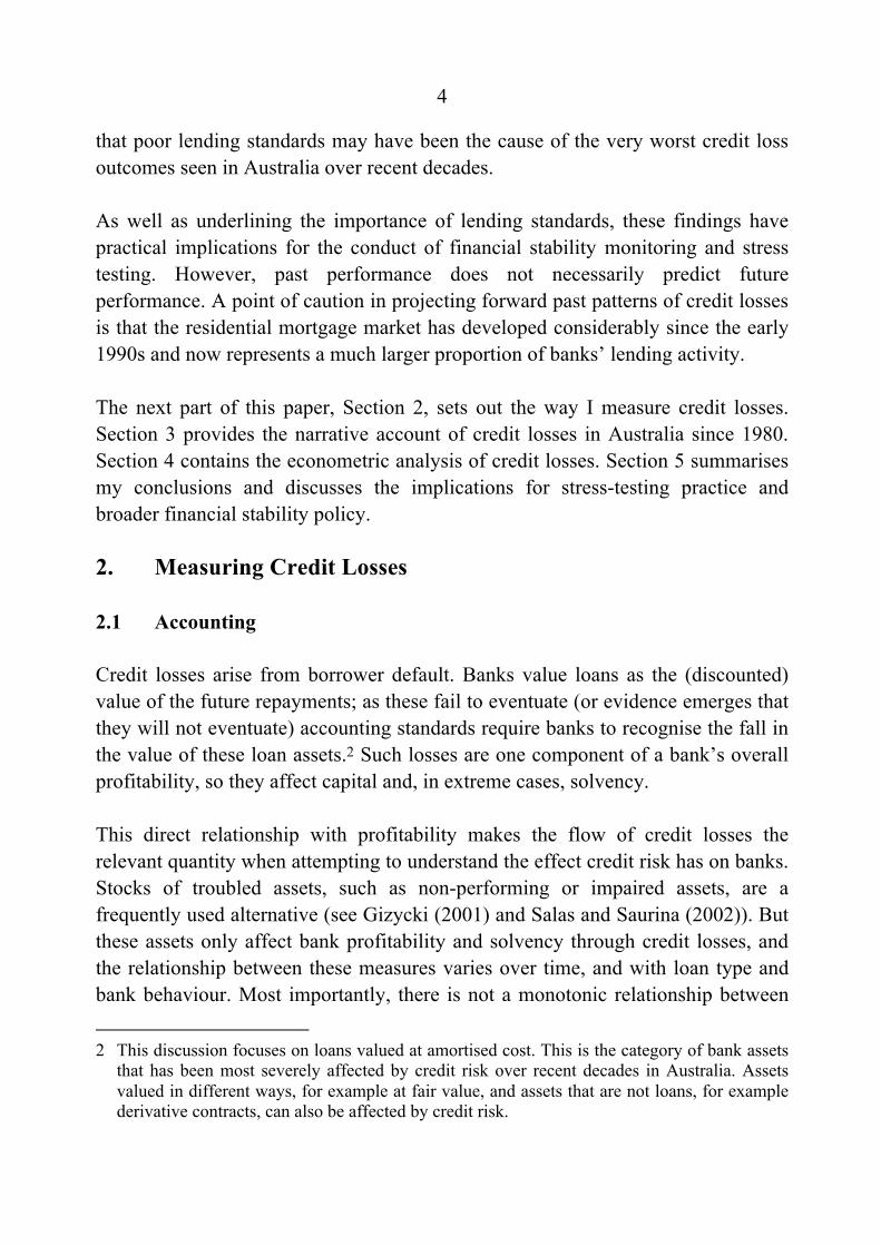
standards also played a role in the different levels of credit losses across these two episodes.

As well as macroeconomic conditions and lending standards, portfolio composition turns out to be important for credit losses. The very limited portfolio-level data available for the early 1990s indicate losses during this episode were incurred mainly on business lending. The better data available for the global financial crisis episode make it clear that the elevated losses during this episode were almost entirely incurred on business lending. Credit losses on housing loans during the global financial crisis episode were minimal.

Other authors have applied econometric models to the ex post credit risk experience of Australian banks. Gizycki (2001) modelled bank-level measures related to credit losses – impaired asset and return-on-asset ratios – over periods that end in 1999. She found the interest burdens of the household and business sectors, real credit growth, the real interest rate, the share of construction in GDP, as well as commercial and residential property prices, to be the macro-level conditions that influenced credit risk measures. This is informative, but the dependent variables that Gizycki used do not have straightforward relationships with credit losses, so these conclusions are not directly transferable to credit losses.1 Hess, Grimes and Holmes (2009) did model credit losses, but did not consider some of the macro-level variables that Gizycki found to play key roles, particularly financial variables. Esho and Liaw (2002) is the only paper on credit losses in Australia that considers banks’ portfolio composition. These authors use measures of portfolio composition from capital data as stand-alone explanatory variables in a model for credit losses over 1991–2001. They found residential mortgage lending to be indistinguishably risky from bank lending to governments, and much less risky than lending to businesses and (non-housing) personal lending.

The econometric models of banks’ credit losses in this paper add to past Australian work in several ways. As the new dataset covers 1980–2013, they include both the early 1990s episode and the global financial crisis. They also consider a wide range of macro-level variables as potential explanators of credit losses. Most importantly, the main econometric model presented in this paper allows the effect of macro-

1 As an example, impaired assets are not a sufficient statistic for credit losses. See Section 2.1

below.

3

level variables on bank-level credit losses to vary depending upon each bank’s portfolio composition. An example of the underlying intuition is that a fall in the profitability of the business sector should lead to more credit losses (as a share of each bank’s lending) for banks with a higher share of their portfolio devoted to business lending. This variability is achieved using interactions between bank-level portfolio composition variables and macro-level variables. This modelling strategy exploits the panel nature of the newly compiled credit loss dataset, as well as that of a regulatory dataset – the bank-level data underlying the aggregate measures of business, housing and personal credit. Interaction variables are clearly suggested by the available data on portfolio-level loss rates – which indicate losses on different portfolios respond differently to macro-level conditions – but a systematic approach of this type is novel in the literature. Pain (2003), Gerlach, Peng and Shu (2005) and Glogowski (2008) allow interactions between the share of one portfolio and a limited number of macro-level variables; I interact all macro-level variables with portfolio shares.

This model with portfolio interactions explains bank-level credit losses over recent decades reasonably well. The macro-level conditions that are statistically and economically significant are business sector conditions. As these variables are interacted with the shares of each bank’s portfolio made up by business lending, this indicates business lending has been the main source of credit losses over recent decades. Analogous interactions between household sector conditions and the shares of banks’ portfolios made up by housing or personal lending are not significant in the model. This result is consistent with the narrative account of credit losses in Australia over this period.

The econometric models in this paper do not explain all of the variation in credit losses. For example, they cannot explain why credit losses were so large at several state government-owned banks during the early 1990s. This accords with the omission of most of the variation in lending standards – roughly, the average riskiness of a bank’s borrowers – from the models (quantitative measures that comprehensively summarise bank lending standards are not available). It also accords with anecdotal evidence that state government-owned banks had below-average lending standards. An alternative measurement strategy, based on quantile regressions, indicates that credit losses at banks with similar portfolios can respond very differently to macro-level downturns, providing further support for the importance of lending standards. While this evidence is not definitive, it suggests

4

that poor lending standards may have been the cause of the very worst credit loss outcomes seen in Australia over recent decades.

As well as underlining the importance of lending standards, these findings have practical implications for the conduct of financial stability monitoring and stress testing. However, past performance does not necessarily predict future performance. A point of caution in projecting forward past patterns of credit losses is that the residential mortgage market has developed considerably since the early 1990s and now represents a much larger proportion of banks’ lending activity.

The next part of this paper, Section 2, sets out the way I measure credit losses. Section 3 provides the narrative account of credit losses in Australia since 1980. Section 4 contains the econometric analysis of credit losses. Section 5 summarises my conclusions and discusses the implications for stress-testing practice and broader financial stability policy.

2. Measuring Credit Losses

2.1 Accounting

Credit losses arise from borrower default. Banks value loans as the (discounted) value of the future repayments; as these fail to eventuate (or evidence emerges that they will not eventuate) accounting standards require banks to recognise the fall in the value of these loan assets.2 Such losses are one component of a bank’s overall profitability, so they affect capital and, in extreme cases, solvency.

This direct relationship with profitability makes the flow of credit losses the relevant quantity when attempting to understand the effect credit risk has on banks. Stocks of troubled assets, such as non-performing or impaired assets, are a frequently used alternative (see Gizycki (2001) and Salas and Saurina (2002)). But these assets only affect bank profitability and solvency through credit losses, and the relationship between these measures varies over time, and with loan type and bank behaviour. Most importantly, there is not a monotonic relationship between 2 This discussion focuses on loans valued at amortised cost. This is the category of bank assets

that has been most severely affected by credit risk over recent decades in Australia. Assets valued in different ways, for example at fair value, and assets that are not loans, for example derivative contracts, can also be affected by credit risk.

5

the measures. If one bank displays a higher level of non-performing assets than another bank during a year, this does not necessarily mean that the first bank experienced a higher level of credit losses during the year.3

In terms of accounting, there are three different ways in which banks can deal with credit losses:

1. The most common way is to create an individual provision, a liability, equal in value to the expected credit loss.4 This liability, and the loan (an asset) from which the credit loss stems, are intended to have a net value equal to the amount the bank expects to recover. The creation of the individual provision is funded through an expense item on the bank’s statement of profit and loss. Provisions are generally raised immediately after a bank receives evidence that it is likely to incur a credit loss. The final stage of the credit loss process – the removal (or write-off) of the loan and accompanying provision from a bank’s balance sheet – often occurs well after this, once the amount of the loss is known with more certainty. This final step does not affect profitability, as the credit loss has already been incurred through the creation of the provision. If the quantum of the loss increases from that expected when the provision was raised, the amount of the individual provision can be increased, or the additional loss can be written-off directly to the profit and loss (see below).

2. Individual provisions are mainly used for credit losses on larger loans. For smaller loans, where it is not economic to assess the likely size of a credit loss at the loan level, banks raise collective provisions. These can be raised to cover, for example, expected credit losses on all small personal loans more than 90 days in arrears. The amount of the collective provision is usually based on past experience – for example, the average credit loss incurred on a particular

3 This may be because the first bank’s non-performing assets were residential mortgages, which

are normally more highly collateralised than other types of lending. Alternatively, the second bank may simply have written off its non-performing assets more quickly than the first bank, in an attempt to display a healthier loan book to investors and ratings agencies.

4 Under the Australian equivalents to the International Financial Reporting Standards (IFRS), ‘provisions’ are liabilities used to lower the value of loan assets to their recoverable value. In the credit losses literature, this term is commonly used for the flow of credit losses (an expense), reflecting its meaning under US Generally Accepted Accounting Principles. Prior to the adoption of IFRS in Australia, individual provisions were called specific provisions, and collective provisions were called general provisions.

6

category of loans in the past. Collective provisions are also used to cover likely future losses on the currently healthy portion of banks’ loan books. Historically, this component of collective provisions has fluctuated in line with banks’ expectations around future credit losses, creating a wedge between losses banks have accounted for through their profit and loss statement, and those that have actually occurred.5

3. Credit losses can also be dealt with without raising provisions; they can be written-off directly to the profit and loss. This method can be used for loans where there is no prospect of recovering a significant portion of the loan amount, or if the quantum of the credit loss is immediately reasonably certain. It is often also used for lending where a high loss rate is expected and built into the interest margin (credit card lending is one example). Unlike where provisions have previously been raised, this type of write-off affects profitability.

This is a simplified overview of the accounting items that are needed to capture a bank’s credit losses. Appendix A provides a complete list of the items needed to accurately measure credit losses. It also provides a detailed example of the accounting for a credit loss on a single hypothetical loan.

Most banks have, over time, used a combination of the above three methods to account for credit losses. I combine credit losses accounted for using the three methods above into three different aggregate measures of the overall credit losses incurred by a bank (the dashed lines in Figure 1). These three aggregate measures differ in the stage at which they capture credit losses accounted for under the three methods. Each has advantages and disadvantages:

• Charge for bad and doubtful debts (CBDD) – This is the aggregate credit risk expense item that appears on banks’ profit and loss statements. It is the net impact of credit risk on profitability, so is the most economically relevant measure. The weakness of this measure is that, as it captures the net charge to the profit and loss to fund collective provisions, it fluctuates in line with a bank’s expectations around future credit losses on currently healthy loans.

5 The adoption of IFRS in 2006 constrained the extent to which Australian banks could raise

collective provisions to cover future loan losses. However, they still do this to some extent. This is dealt with in Appendix B.

7

• Current losses (CL) – This measure modifies the CBDD in an attempt to capture only losses that have actually occurred. Instead of using the net charge to profit and loss to fund collective provisions, it includes only write-offs against these provisions. This change is intended to exclude provisions raised to cover likely future losses on currently healthy loans.

• Net write-offs (NWO) – This captures write-offs against all provisions, as well as write-offs made directly to the profit and loss. It is less subjective than the CBDD and CL, because write-offs are usually made significantly after initial loss recognition, when the quantum of credit losses is more certain. But this long lag means that NWO lag the CBDD and thus the economic impact of losses on banks.

Figure 1: Accounting for Credit Losses

These dollar measures need to be scaled to be comparable across years. Following standard practice, I look at losses during each year as a share of loans outstanding at the start of the year (Foos, Norden and Weber 2010). This prevents mechanical exaggeration of loss rates by loan losses during a year lowering measured lending at the end of a year. I call the three resulting ratios the ‘bad debt ratio’ (CBDD/net lending), ‘current loss ratio’ and ‘net write-off ratio’, and denote them by (respectively) BDR, CLR and NWOR. The CLR is the focus of my analysis, as it

Net write-offs

Charge for badand doubtful debts

Current losses

A c

redi

t los

s on

a lo

an

1Raise individual

provision[impact on profit]

Write-off loan andindividualprovision

[no impact on profit]

2Raise collective

provision[impact on profit]

Write-off loan andcollectiveprovision

[no impact on profit]

3Write-off directlyto profit and loss[impact on profit]

8

provides a compromise between timeliness of economic impact and accuracy in measuring actual losses.6

2.2 Data

The main credit loss dataset used in this paper was largely compiled from banks’ annual financial reports. This (public) source is the only one that provides credit losses right back to 1980 – collection of credit loss data by prudential regulators started later.7 The dataset only covers whole-of-bank credit losses, rather than credit losses broken down by portfolio, as these are only available for a broad range of banks from 2008. The data is for parent banks, rather than consolidated groups. Parent bank data exclude lending by overseas subsidiaries, allowing me to concentrate on the credit risk from Australian loans.8 Banks were chosen for the sample by looking at the ten largest banks at five-year intervals from 1980 to 2010; attempts were made to gather data over the full period for any bank that was in the top ten for any sub-period. The resulting dataset covers 26 banks, and is slanted towards larger banks (see Appendix B for a list of included banks). It is unbalanced, as banks enter, exit, and merge. On average, it covers around 80 per cent of bank lending in Australia over the sample period (Figure 2).

Where useful, I employ other credit risk data. For example, I use the portfolio-level (i.e. business, housing and personal) loss rates that the major banks have published in their (publicly available) Pillar 3 reports since 2008. I also make use of regulatory datasets, such as the long-run non-performing assets data (available from June 1990) and the quarterly credit loss data (available from 2003).

The major non-credit risk dataset used in this paper is the micro data underlying the measures of aggregate credit provided by financial institutions in Australia. This provides the share of each bank’s lending that is devoted to business, housing, and personal lending at each point in time.

6 Current losses are the measure used for Australian banks by Esho and Liaw (2002), though

these authors calculate and present it quite differently. 7 I use regulatory data to measure the credit losses of three (unlisted) banks from 2002 onwards. 8 This choice also excludes lending by banks’ domestic finance company and merchant bank

subsidiaries, many of which experienced substantial credit losses during the early 1990s.

9

Figure 2: Sample Coverage As at September

Sources: Annual reports; APRA; RBA

3. Descriptive Analysis

3.1 Credit Losses over Recent Decades

The Australian bank credit loss experience since 1980 is dominated by the very high rate of losses before, during, and after the early 1990s recession, as well as the smaller losses during and after the global financial crisis (Figure 3). Losses around the early 1980s recession were much lower. Relative to lending, credit losses during the early 1990s far exceeded those incurred by banks during and after the global financial crisis. Current losses between September 1989 and September 1994 totalled around 8½ per cent of the average value of banks’ lending during this period. In comparison, current losses during September 2007 to September 2012 were equivalent to around 2½ per cent of average lending over this period.

1983 1989 1995 2001 2007 20130

5

10

15

0

25

50

75

Share of bank lending(RHS)

no %

Number of banks (LHS)

10

Figure 3: Credit Losses and Output Growth Sample aggregate, as at September

Sources: ABS; Annual reports; APRA

The average sample aggregate CLR during 1980–2013 was 56 basis points. The median, less influenced by the high levels in the early 1990s, was 34 basis points, which was also the 2013 level.

Credit losses have strongly influenced the profitability of the Australian banking system during the sample period. This can be seen by decomposing changes in aggregate return on equity, a common measure of bank profitability (Figure 4).9 Credit losses were the largest contributor to the cycles in profitability during the early 1990s and global financial crisis episodes.10

9 The data used in this exercise differ somewhat from the credit losses dataset: it is consolidated

data for Australian-owned banks only. 10 Decomposing changes in a ratio requires choices as to the ordering of the decomposition. I

have used the ordering that minimises the contribution of credit losses to the change.

-2

0

2

4

-1

0

1

2

%

2013

%

GDP growth(LHS, year-average)

Bad debtratio

(RHS)

Current loss ratio(RHS)

Net write-off ratio(RHS)

20072001199519891983

11

Figure 4: Bank Profitability and Credit Losses Australian-owned banks, consolidated data, as at September

Source: Annual reports

3.1.1 The early 1990s

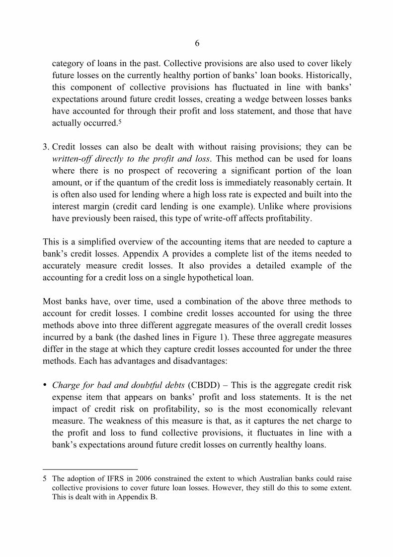
The partial portfolio-level data that are available for the early 1990s episode indicate that the bulk of credit losses were incurred on lending to businesses rather than households. Two major banks published usable portfolio breakdowns of their net write-offs in their annual reports for some or all of the early 1990s, but the categories used in this data were not well defined (Figure 5).11 They show losses on non-construction housing loans were minimal (these fall within the ‘Real estate – mortgage’ category). Loans to individuals for construction of housing probably fell within the ‘Real estate – construction’ category, but this category also contains lending for commercial property. Losses on this category were significant, but only make up around 13 per cent of reported losses for these two banks. The key point is that most of the losses reported by these two banks fall in the ‘Other business’ category. Losses on personal lending, such as credit cards and non-housing term loans, were non-negligible, but appear to be less cyclical than losses on business lending.

11 These two banks, CBA and NAB, accounted for 33 per cent of bank lending at

September 1991. CBA’s write-offs include those made within the State Bank of Victoria’s loan book after its acquisition in November 1990.

0

10

20

0

10

20

1987 1992 1997 2002 2007 2012-20

-10

0

10

-20

-10

0

10

Due to other components

%Return on equity

Change in ROE

Due to credit losses

Total change

%

%

%

12

Figure 5: Write-offs by Portfolio – Two Major Banks

Note: (a) Mainly owner-occupied housing lending

Source: Annual reports

Portfolio-level data are available on all banks’ non-performing assets from mid 1990 to mid 1994, and these support the conclusion that losses were incurred mainly on business lending (Figure 6).12 It shows that the share of banks’ lending to businesses that was non-performing far exceeded the share of their lending to households (including non-mortgage personal lending) that was non-performing.

12 No similar data were collected before June 1990, and the regulatory collection from

September 1994 onwards did not have a portfolio breakdown. These rates are slightly downward biased. The numerator uses non-performing assets data from the Australian operations of all banks’ consolidated groups. In contrast, the denominator includes all lending done by financial intermediaries in Australia, including lending done by non-bank financial companies not owned by banks.

150

300

450

600

150

300

450

600

1989 1990 1991 1992 1993 1994 19950

300

600

900

0

300

600

900

NAB – net

CBA – gross

$m

$m

$m

$m

1 2001 200

nana

Personal Real estate – mortgage(a) Real estate – construction Other business

13

Figure 6: Non-performing Assets by Portfolio All banks, share of lending by type

Source: RBA

Contemporary accounts of the period also indicate that credit losses were primarily on lending to businesses. Trevor Sykes’ (1994) classic account of corporate and banking collapses during this period, The Bold Riders, is one example. Edna Carew’s (1997) account of Westpac’s experience during the period indicates its losses were concentrated in business lending, and more specifically, in property development lending. The dominant role of business lending is also suggested by contemporary accounts from industry participants (Phelps 1989; Lee 1991).

Various authors have set out potential reasons why credit losses were so large in the early 1990s (Battellino and McMillan 1989; Fraser 1994; Sykes 1994; Carew 1997; Conroy 1997; Ullmer 1997; Gizycki and Lowe 2000). There was a recession during 1990–91, and downturns in financial and property markets, but losses were many times greater than those seen in earlier (and later) downturns, suggesting other factors at play. A short version is that deregulation of the banking sector in the 1980s was accompanied by very fast business lending growth and declining lending standards, all during a period of strong economic and financial

0

4

8

12

0

4

8

12

Lending to businesses

1994

%%

Lending to households

1993199219911990

14

conditions.13 When conditions eventually worsened, a sharp rise in credit losses was the result. In more detail:

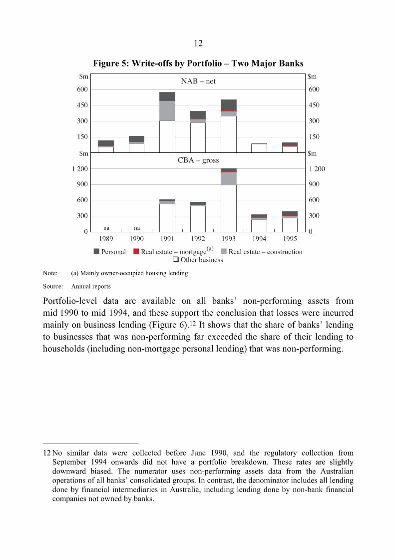
1. Deregulation allowed banks to extend credit to meet demand from borrowers (Battellino and McMillan 1989). The rates and terms at which banks could offer deposits were liberalised over the 1970s and first half of the 1980s. Prior to this, banks passively accepted deposit flows and restricted lending during periods of deposit outflow. The change allowed banks to actively manage their funding to match the demand for credit, and was accompanied by the removal of interest rate caps on lending products and requirements for banks to lend to certain borrowers. In addition, in 1985 foreign banks were allowed to enter the Australian banking market as retail deposit-takers for the first time in over 40 years (Fraser 1994). The net result of these changes was a market where banks competed intensely to grow their loan books and maintain market share. Annual growth in nominal business credit rose above 20 per cent in September 1984, and didn’t fall below this level again until June 1989 (Figure 7).

13 I use a broad definition of lending standards in this paper: non-price differences in borrower

characteristics and loan terms that are ex ante observable by a bank. I expand on this definition below, but it is important to note that I do not include changes in portfolio composition between business, housing, and personal loans within my definition.

15

Figure 7: Business Credit Growth Year-ended

Note: (a) Deflated using the domestic final demand deflator

Sources: ABS; APRA; RBA

2. In part due to the competitive pressures unleashed by deregulation, bank lending standards loosened considerably over the 1980s (Macfarlane 1991; Sykes 1994; Conroy 1997; Ullmer 1997). From the late 1970s, banks departed from the practices of earlier decades and began lending to large companies on an unsecured basis, and accepting riskier forms of collateral (such as equity in subsidiaries and mortgages over unfinished developments). Banks also relaxed covenants around the use of borrowed funds, loan-to-valuation and interest-coverage ratios. Another major driver of the losses over this period was a lack of transparency on borrowers’ total use of debt finance. When borrowers entered financial difficulty, banks would sometimes discover total debt was higher than thought, and even their own group exposures were higher than thought, due to lending by subsidiary finance companies and merchant banks. Remuneration was one potential driver of the fall in lending standards: corporate lending officers in banks were frequently remunerated on the basis of volume, with little consideration of long-run asset performance. Arguably, this loosening of lending standards occurred because banks, emerging from an era of tight regulation, lacked the proper corporate governance and sophisticated credit risk

-10

0

10

20

30

-10

0

10

20

30

2013

%%

20072001199519891983

Nominal

Real(a)

16

management frameworks that have come to be seen as necessary for prudent banking in a deregulated financial system.

3. Macroeconomic and financial conditions facilitated these developments. Real GDP grew at an average rate of about 4¼ per cent over the five years to September 1989. Equity prices rose by almost 50 per cent per annum from late 1984 until the crash in October 1987. Commercial property price growth rose above 10 per cent per annum at the start of 1986, and accelerated in subsequent years. This price growth was accompanied by an exceptional amount of non-residential construction, particularly of offices (Figure 8; Kent and Scott 1991). Commercial property was a key form of collateral for the business loans that were secured.

Figure 8: Office Construction and Price Growth

Note: (a) Capital city CBD prices: based on Adelaide, Melbourne, Perth and Sydney prior to June 1984,

includes Brisbane and Canberra after

Sources: ABS; JLL Research; RBA

4. Immediate triggers for the rise in credit losses are easier to discern than the underlying reasons why they were so large. Business interest rates rose from around 13 per cent at the start of 1988 to over 20 per cent by the end of 1989, due to rises in official rates. Together with slowing business profits growth and the significant growth in business debt, this meant that the aggregate business

0.0

0.3

0.6

0.9

-50

-25

0

25

Office construction(LHS, per cent of GDP)

2013

%%

Office price growth(a)(RHS, year-ended)

20072001199519891983

17

sector interest burden was very high (Figure 9). By early 1990, large highly geared companies across a range of industries were unable to meet their increased loan repayments and defaulted on their debts (Sykes 1994). This, together with a weakening in the commercial property market, exposed banks to a first round of credit losses (Gizycki and Lowe 2000). These losses broadened as business profits began to fall and Australia entered a recession around the end of the year. By September 1991, large additions to the supply of office property had combined with flat or falling demand to sharply raise vacancy rates and drive prices down by over 20 per cent on an Australia-wide basis; some banks were forced to recognize significant credit losses on commercial property lending (Carew 1997).

Figure 9: Business Sector Conditions and Credit Losses

Note: (a) Business sector interest payments on intermediated debt divided by profits

Sources: ABS; Annual reports; APRA; RBA

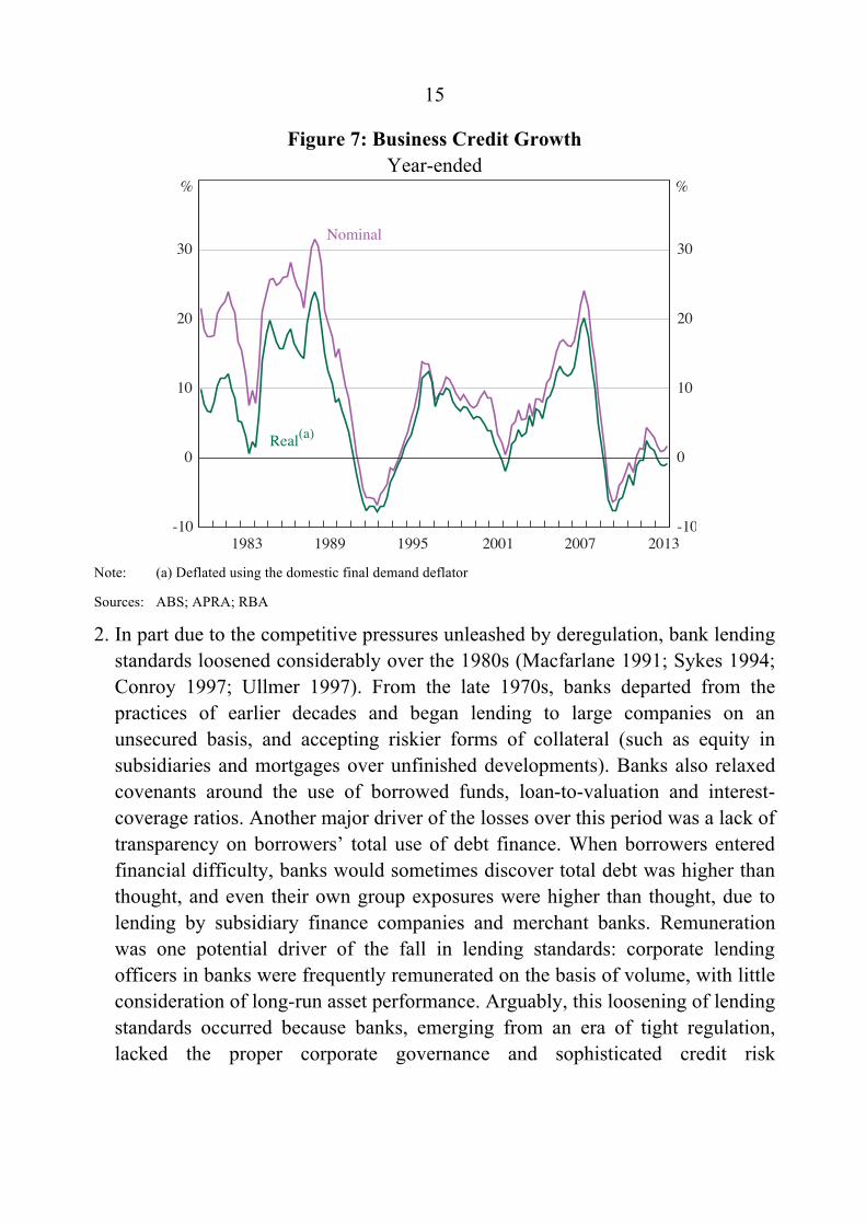
Of the banks in the long-run dataset, the one that incurred the highest rate of credit losses during the early 1990s was a small foreign-owned bank (Figure 10). These losses were equivalent to a significant proportion of this bank’s capital, but it was recapitalised by its parent entity. Of the groups that make up larger portions of the sample, state government-owned banks experienced the highest credit loss rates over this period. Two, the State Bank of South Australia (SBSA) and the State Bank of Victoria (SBV), effectively failed, in that they had to rely on extraordinary

0

15

30

0

15

30

1983 1989 1995 2001 2007 20130

1

2

3

0

1

2

3

Profits growth%

Current loss ratioSample aggregate, as at September

Business sector conditions %

%

%

Average interest rate

Interest burden(a)

18

financial support from their state government owners (Fitz-Gibbon and Gizycki 2001). The major banks also experienced large credit losses over this period. Two major banks – Westpac and ANZ – reported large overall losses in their annual reports for 1991. The other banks in the sample, primarily smaller Australian-owned banks, incurred significantly lower losses over the period. These banks’ portfolios were generally more concentrated in lending to households.

Figure 10: Bank-level Credit Losses Individual bank current loss ratios, as at September

Source: Annual reports

Even during a period in which system-wide lending standards loosened, there are indications lending standards at state government-owned banks, particularly SBSA and SBV, were below average:

• These banks grew their lending very quickly over the late 1980s. SBSA and SBV grew their lending at rates of 43 and 27 per cent per year between 1985 and 1990, versus growth in total credit of around 18 per cent per year over this period. This fast growth was driven by business lending – the share of these banks’ portfolios made up by business lending increased by over 20 percentage points over the same period. State government owners encouraged fast lending growth, both to support state economies and to provide a new source of revenue for state coffers, and installed aggressive managers (Sykes 1994).

0

2

4

6

8

10

0

2

4

6

8

10Foreignbanks

2000

%%

19961992198819841980

State government-ownedbanks

Other banks

19

• There is some direct evidence on lending standards at these institutions. The Auditor-General of South Australia’s report into SBSA stated:

… the Bank’s corporate lending … was poorly organised, badly managed and badly executed. Credit risk evaluation was shoddy. Corporate lending policies and procedures were not even compended into a credit policy manual until 1988, and even then contained serious omissions. The ultimate loan approval authority - the Board of Directors - lacked the necessary skills and experience to perform its function adequately. Senior management’s emphasis was on doing the deal, and doing it quickly. (MacPherson 1993, p 1-24)

• State government-owned banks were not formally subject to prudential supervision by the Reserve Bank, though they had given undertakings to comply with the Reserve Bank’s prudential regulations. Despite this, there were instances where they did not do so.14

Despite large credit losses, there were no disorderly bank failures during the early 1990s (Gizycki and Lowe 2000). The liabilities of state government-owned banks were always explicitly guaranteed by their owners. The banking system as a whole remained well-capitalised; partly due to some banks raising equity, the aggregate capital ratio actually rose over this period (Fraser 1994). Both ANZ and Westpac maintained capital ratios above regulatory minima, despite their losses in 1991. There were short-lived deposit outflows at some small banks, but these were quickly ended by Reserve Bank assurances about their solvency.

3.1.2 The global financial crisis

The elevated credit losses experienced during and after the global financial crisis were due to business lending; the better data available for this period make this clear (Figure 11). Losses on household lending barely rose over the period. Losses on the business loan portfolio were much lower than those incurred during the early 1990s: annual net write-off rates on business lending averaged 0.8 per cent over the four years beginning in March 2009, well-below average total write-offs

14 Sykes (1994) provides the examples of a large exposure and a related-party transaction that

were undertaken by SBSA contrary to Reserve Bank advice. The SBV failed to meet the Reserve Bank’s capital adequacy standards during the late 1980s (Victoria 1991).

20

rates during the early 1990s (and, presumably, even higher business loan write-off rates at that time).

Figure 11: Credit Losses by Portfolio Annual net write-off ratios

Notes: (a) Consolidated data for three major banks

(b) Includes all banks with housing loans > $1 billion; eighteen banks as at December 2013

Sources: APRA; Pillar 3 reports

The low loss rate on lending to households over this period was driven by very low losses on housing loans, which made up around 90 per cent of bank lending to households over this period. The net write-off ratio on housing lending averaged 3 basis points per year during 2008–13.15 Most of the losses on lending to households during this period arose from personal lending (credit card and other personal lending) (Figure 12). Though personal lending has a relatively high loss rate, it appears to be significantly less cyclical than business lending, and anyway only makes up around 5 per cent of bank lending in Australia.

15 This loss rate is after the effect of lenders mortgage insurance (LMI), which Australian banks

hold on a significant portion of their housing loans (estimates suggest LMI covers roughly one-quarter of housing loans). Reserve Bank estimates suggest the annual loss rate faced by lenders mortgage insurers averaged 3 basis points over 1984 to 2012.

0.0

0.2

0.4

0.6

0.8

1.0

1.2Lending to businesses(a)

20130.0

0.2

0.4

0.6

0.8

1.0

1.2

Lending to households(a)

Business and personalloans(b)

Housing loans(b)

%%

20112009201320112009

21

Around one-fifth of Australian-owned banks’ consolidated assets are offshore, so the consolidated Pillar 3 data used in Figure 11 (left panel only) and Figure 12 reflect overseas credit risk to some extent. Australian banks’ credit losses on offshore lending were significant during the GFC (see, for example, RBA (2010)), but domestic credit risk is the focus of this paper.

Figure 12: Credit Losses by Portfolio Consolidated data for three major banks, annual net write-off ratios

Source: Pillar 3 reports

One part of the explanation for the lower credit losses experienced during the global financial crisis is the less severe nature of this episode: GDP fell for only a single quarter and office property prices fell by around a quarter, compared with a peak-to-trough decline of around one-half in the early 1990s (see Figure 8). Bank lending to businesses grew at around 15 per cent per annum over the five years up to mid 2008; this was around 8 percentage points below its growth rate over the five years up to mid 1989 (higher inflation in the earlier period only accounts for around half of this gap). This smaller rise in debt, together with structurally lower interest rates that fell quickly in response to large cuts to the cash rate, meant the business sector’s aggregate interest burden peaked at around 17 per cent of profits during the global financial crisis, well below its level in the early 1990s (see Figure 9).

0

1

2

3

4

0

1

2

3

4

Residential mortgage lending

2013

%%

20122011201020092008

Credit cards

Other personal lending

22

There is also evidence that more conservative business lending standards were a key contributor to the better credit loss experience during this episode. Partly in response to the problems in the early 1990s, and partly in response to the imposition of risk-based capital requirements and other regulatory pressures, banks had improved their management of credit risk by the start of the global financial crisis according to many observers (Eales 1997; Ullmer 1997; Gray 1998; APRA 1999; Laker 2007). Better IT systems were put in place to assess and monitor credit risk, and the governance of credit risk decisions within banks had improved.

3.2 Other Aspects of Credit Losses

This section explores the timing of credit losses with respect to the economic cycle, and relationships between credit risk measures. If credit losses peak quickly after troughs in output, this means the financial strength of the banking sector may start to improve soon afterwards – a key consideration for economic policymakers after the global financial crisis. Likewise, if credit losses peak before non-performing assets, they might provide an early signal of future improvement in the financial strength of the banking sector.

3.2.1 Timing

The temporal relationship between credit losses and output was reasonably similar during the early 1990s and global financial crisis episodes. The peak in current losses in the early 1990s, as measured by the long-run dataset (which provides annual losses as at September of each year), was in 1991. The trough in annual GDP during this episode was in the December quarter of 1991. APRA’s quarterly credit loss data for all banks (available from 2003), allow more precise measurement of timing. Quarterly credit losses, a volatile series, peaked in the same quarter as the trough in quarterly GDP during the global financial crisis episode (Figure 13). Losses rose noticeably three years before their peak in the early 1990s, while they were only slightly elevated a year before their global financial crisis peak.

23

Figure 13: Current Loss Ratio and Output – Timing Peak = 100

Sources: ABS; APRA

3.2.2 Relationships between credit risk measures

The relationships between different measures of credit losses differed somewhat across the two main episodes (see Figure 3). The BDR exceeded the CLR in the years immediately prior to both the downturns, indicating that banks were increasing collective provisions in anticipation of a deterioration in loan performance. During the global financial crisis, banks continued to increase collective provisions during the downturn itself, perhaps owing to an overly pessimistic view of future developments. The profile of credit losses was a relatively symmetric hump in the early 1990s, but credit losses generally declined more slowly in the years following the global financial crisis. This may reflect economic conditions over this period, or banks adjusting their behaviour in recognising and disposing of troubled loans. This difference makes comparing the delay between initial losses and final write-offs between the two episodes difficult; but, in aggregate, the net write-off ratio peaked two years after the other two ratios in the early 1990s, and a year after in the global financial crisis episode.

-8 -6 -4 -2 0 2 4 6 80

20

40

60

80

100

0

20

40

60

80

100

Quarters from trough in GDP

indexindex

Current lossratio – annual

Current lossratio – quarterly

24

Credit losses in Australian banking have generally peaked before non-performing assets (NPA) and impaired assets (IA), though these measures have risen in tandem at the start of downturns. APRA’s quarterly credit loss data for all banks show a lead of three quarters between the peak in annual credit losses and that in NPAs during the global financial crisis episode (Figure 14); the lead is five quarters between the peak in quarterly credit losses and that in NPAs. For IAs, these leads are arguably zero and two quarters (respectively), given the June quarter 2009 value for this variable is very close to its peak in the March quarter of 2010.

Figure 14: Credit Losses and Non-performing Assets All banks

Source: APRA

4. Econometric Analysis

The narrative account in Section 3 reveals a range of features of credit losses in Australian banking. Aggregate credit losses clearly have a relationship with the economic cycle, but appear to be affected by macro-level factors other than just output growth. Business sector conditions, such as commercial property prices and business indebtedness, look to have played the key role. The composition of banks’ portfolios also appears important: credit losses look to have been incurred mainly on business lending. But the direct evidence for this is based on data from only a

0.0

0.2

0.4

0.6

0.8

0.0

0.5

1.0

1.5

2.0

Current loss ratio– annual

(LHS)

2013

%%

2011200920072005

Current loss ratio– quarterly

(LHS)

NPA ratio(RHS)

IA ratio(RHS)

Peak in NPA and IA ratios

25

few banks for the largest episode of credit losses. Cross-sectional differences in bank-level credit losses have been large, and there are suggestions that these are driven by variation in lending standards (as well as portfolio composition). Section 4 uses a panel data modelling framework to explore these issues further.

4.1 Modelling Approach

Consistent with the international literature, I model the relationships between bank-level credit losses and both macro-level and bank-level factors (see Equation (1)).16 I use annual bank-level current loss ratios as the dependent variable (CLRit, where i indexes banks and t years). Following the majority of the literature, I use the fixed-effects (within) estimator, which removes time-invariant bank-level heterogeneity (αi). This is done on the basis that some of this heterogeneity is unobservable and may be correlated with the explanatory variables of interest. Relevant unobservables include the average risk appetite of a bank’s managers and, relatedly, its average lending standards (both of these probably also vary within banks over time, and this is explored in Section 4.4).

it i t itCLR α εʹ′ ʹ′= + + +itβMACRO γ BLEVEL (1)

Macro-level explanatory variables (MACROt) include real GDP growth, growth in business sector profits and growth in the household sector’s disposable income, all measures of changes in borrowers’ incomes. The level of the cash rate, as well as the interest burdens of the whole economy, household sector and business sector, are included as more precise measures of borrowers’ ability to repay their loans.17 System-wide nominal credit growth, and growth in nominal housing and business credit, are intended to capture system-wide changes in lending standards (see, for example, Keeton (1999)). Residential and commercial property are used as collateral for housing and business loans in Australia, so changes in the prices of these assets are included to capture changes in the value of this collateral. Details

16 A survey is available in Glogowski (2008). Salas and Saurina (2002) are a commonly cited

precedent when using macroeconomic and bank-level explanatory variables to model bank-level credit risk outcomes.

17 The economy-wide interest burden is equal to the estimated interest payments on all intermediated debt in the economy divided by GDP. The business and household sector interest burdens are defined similarly: see Table B2.

26

of variable construction, descriptive statistics and correlations for all explanatory variables are in Appendix B (Tables B2, B3 and B4).

Bank-level variables (BLEVELit) include the shares of each bank’s portfolio devoted to business and personal lending, and bank-level loan growth.

I include all variables contemporaneously, except for interest burden (which I lag one year) and the credit and loan growth variables (I include lagged terms covering the past four years for these variables). These variables are excluded contemporaneously because of the mechanical impact of credit losses on the level of credit and loans (these measures are calculated net of identified losses). I exclude bank-year observations on banks making up less than 1 per cent of total bank loans to prevent idiosyncratic risk in very small loan portfolios from clouding my results. This leaves 328 observations on 26 banks covering 1982 to 2013.

4.2 Initial Models

Table 1 reports regression results from two alternative forms of Equation (1). Model A uses mainly economy-wide macro-level explanatory variables. Model B uses variables specific to the household and business sectors.

These models indicate that the drivers of credit losses over 1982–2013 are largely those highlighted by previous Australian work using shorter time periods. At the macro level, interest burdens, sectoral credit growth measures, and growth in residential and commercial property prices appear to influence losses, and measures specific to both the business and household sectors appear important. These results are entirely consistent with Gizycki (2001), who modelled ex post credit risk at Australian banks over periods ending in 1999. Banks with mainly business lending appear to have incurred higher credit loss rates than banks with mainly housing lending, in line with Esho and Liaw (2002). The model that uses only sectoral macro-level variables (Model B) explains credit losses slightly better than the one that uses primarily economy-wide variables (Model A). This is useful for the development of the main model of this paper – presented in Section 4.3 – which includes interactions between portfolio shares and macro-level variables.

27

Table 1: Initial Models Dependent variable = CLR

Variable Model A Model B Macro-level GDP growtht –0.063* Business profits growtht –0.041*** Household disposable income growtht –0.006 Cash ratet –0.007 Economy-wide interest burdent – 1 0.137*** Business sector interest burdent – 1 0.062** Household sector interest burdent – 1 0.144*** Commercial property price growtht –0.020*** –0.006 Residential property price growtht –0.016*** –0.012*** Credit growtht – 1 –0.012 Credit growtht – 2 –0.023 Credit growtht – 3 0.026 Credit growtht – 4 –0.024 Business credit growtht – 1 –0.028*** Business credit growtht – 2 –0.007 Business credit growtht – 3 0.028* Business credit growtht – 4 –0.019* Housing credit growtht – 1 0.032*** Housing credit growtht – 2 0.013 Housing credit growtht – 3 –0.025 Housing credit growtht – 4 0.007 Constant –1.576*** –2.749*** Bank-level Business share of lendingt – 1 2.087** 2.241** Personal share of lendingt – 1 3.254*** 3.337*** Loan growtht – 1 0.009 0.006 Loan growtht – 2 0.008* 0.005 Loan growtht – 3 0.001 0.001 Loan growtht – 4 0.013** 0.011** Observations 328 328 Within R-squared 0.48 0.54 Adjusted within R-squared 0.45 0.51 AIC 725 697 BIC 785 781 Notes: All models are estimated with bank fixed effects and standard errors are clustered by bank; ***, ** and *

denote significance at the 1, 5 and 10 per cent level respectively

28

These simple models offer a number of other insights:

• Looking first at the proxies for borrower income, GDP growth is intuitively signed, but only significant at the 10 per cent level. Output growth has been found insignificant in international studies using models that include a range of cyclical macro-level variables (Davis and Zhu 2009). At the sectoral level, business profits growth has a negative relationship with credit losses that is significant at the 1 per cent level, while growth in household disposable income does not appear to be a significant explanator of credit losses. This difference is consistent with the relative importance of developments in these sectors in the narrative account of credit losses in Australia.

• The economy-wide interest burden has a statistically significant relationship with credit losses in Model A. A one standard deviation increase in this variable (roughly 2 percentage points) is associated with a 26 basis point rise in credit loss ratios. The economy-wide aggregate interest burden is the weighted average of borrower-level interest burdens across the economy; a rise in the former must represent some increase in risk at the borrower level. Interest burdens within both the business and household sectors appear to underlie this aggregate relationship – both are significant in Model B. This is consistent with Gizycki (2001), but is not consistent with the narrative account of credit losses in Australia. Default and financial distress among household borrowers does not feature prominently in this.

• Both residential and commercial property price growth appear to influence bank credit losses. Again, while consistent with Gizycki (2001), this is not entirely consistent with the narrative account of credit losses in Australia. Residential property has primarily served as collateral for housing loans in Australia, and the available evidence indicates banks have not incurred significant credit losses on such loans over recent decades. Residential property now also collateralises a significant amount of small business lending in Australia, but this makes up only a small proportion of total business lending and it is unclear how prevalent this arrangement was in earlier decades.

• Business credit growth and housing credit growth are important for credit losses in this model, though they have opposite effects over short horizons. Positive relationships between longer lags of credit and loan growth and losses are the

29

most common finding in the international literature, and are generally thought to operate through increases in credit supply that involve lending to less financially sound borrowers (see Section 4.4). Though there is an explanation for the estimated negative relationship between business credit growth and losses – more easily available credit (signalled by strong credit growth one year ago) may make refinancing easier for weaker borrowers who would otherwise default – this estimated relationship should be interpreted cautiously. Demand for credit probably weakens during downturns (which in turn cause credit losses), so the estimated relationship may not be causal.

• At the bank level, portfolio composition has statistically significant effects with relative magnitudes that accord with the portfolio-level loss rates shown in Section 3.1.2. A bank with more business lending and less housing lending incurs higher credit losses. More (non-housing) personal lending has a similar, but stronger, effect. Higher loan growth raises losses at the individual bank level with a multi-year lag. The estimated coefficients on this variable are of a similar magnitude to those found by Hess et al (2009) for Australian banks.

4.3 Using Portfolio Composition

This section contains the primary econometric model for credit losses presented in this paper. It uses the same modelling framework as the simple models presented in Section 4.2, but relies on explanatory variables that are interactions between macro-level variables and bank-level portfolio shares. Equation (2) shows a model of this type: BSLit – 1 is the share of bank i’s lending that was business lending at t – 1, and MACRO1t contains macro-level variables likely to affect credit losses on business lending (HSLit – 1 and MACRO2t are defined analogously for housing lending, and PSLit – 1 and MACRO3t for personal lending). The model uses all of the macro-level variables in Model B above. Those assigned to MACRO1t are simply those thought to cause credit losses on business lending: business profits growth, the business sector interest burden, business credit growth, and commercial property price growth. The other macro-level variables – those that capture the conditions in the household sector – are present in both MACRO2t and MACRO3t, except for housing credit growth, which is in MACRO2t only.

1 1

1

it i it t it t

it t it

CLR BSL HSLPSL

α

ε− −

−

ʹ′ ʹ′= + +

ʹ′ ʹ′+ + +

1 23

β

γ it

MACRO MACROK MACRO BLEVEL

Γ (2)

30

The key idea is that requiring macro-level variables to affect credit losses through the portfolios they are related to should provide better identification of the drivers of credit losses. For example, the mechanism through which falls in residential property prices are thought to cause credit losses is by lowering the value of the collateral backing housing loans. A model that requires changes in residential property prices to act on credit losses through banks’ housing lending should distinguish this causal channel from mere correlation between house prices and other macro-level conditions that cause credit losses (cross-correlations between my explanatory variables are shown in Appendix B). The limited international literature that models credit losses at the portfolio level generally finds each portfolio has a different relationship with macro-level conditions.18

A necessary condition for the unbiased estimation of Equation (2) is that the portfolio shares are independent of the error term. One reason why this assumption may not hold is correlation between (within-portfolio) lending standards and portfolio shares. But arguments can be made for both positive and negative relationships; banks that do more business lending should be better at selecting businesses to lend to, but banks with a lot of business lending may have arrived at that position by accepting borrowers other banks did not. The dataset contains a wide range of variation in portfolio composition, in part due to the regulatory distinctions between savings banks (which mainly concentrated on housing lending) and trading banks (which mainly concentrated on business lending) over the late 1980s and early 1990s. The state government-owned banks that received extraordinary government support in the early 1990s had shares of business lending in the middle of the sample range.

Table 2 shows the estimation results from the model (Model C). The key insight from Model C is that business sector conditions appear to have been the main driver of credit losses in Australia over recent decades. The household sector interest burden, residential property prices, and housing credit growth no longer

18 For example, using data on Greek banks, Louzis, Vouldis and Metaxas (2012) found non-

performing personal loans to be very sensitive to interest rates, business lending sensitive to GDP growth, and mortgages not very sensitive to macroeconomic developments. Hoggarth, Logan and Zicchino (2005) estimate models for sectoral write-offs from UK banks’ business, personal, and housing portfolios that are each driven by a different set of macro-level variables.

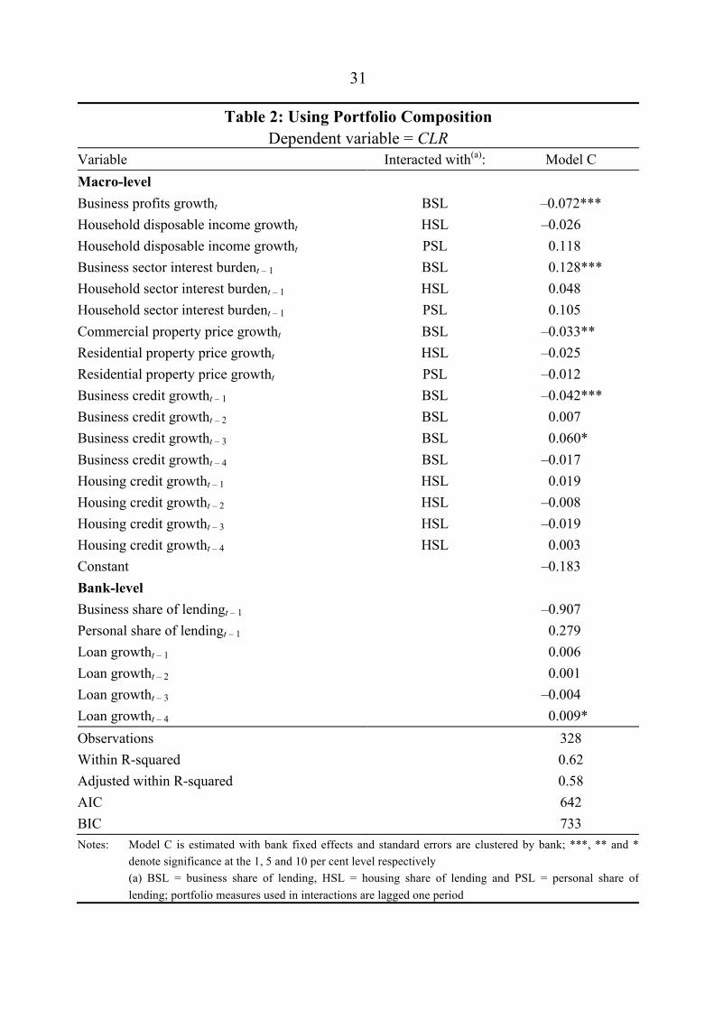
31

Table 2: Using Portfolio Composition Dependent variable = CLR

Variable Interacted with(a): Model C Macro-level Business profits growtht BSL –0.072*** Household disposable income growtht HSL –0.026 Household disposable income growtht PSL 0.118 Business sector interest burdent – 1 BSL 0.128*** Household sector interest burdent – 1 HSL 0.048 Household sector interest burdent – 1 PSL 0.105 Commercial property price growtht BSL –0.033** Residential property price growtht HSL –0.025 Residential property price growtht PSL –0.012 Business credit growtht – 1 BSL –0.042*** Business credit growtht – 2 BSL 0.007 Business credit growtht – 3 BSL 0.060* Business credit growtht – 4 BSL –0.017 Housing credit growtht – 1 HSL 0.019 Housing credit growtht – 2 HSL –0.008 Housing credit growtht – 3 HSL –0.019 Housing credit growtht – 4 HSL 0.003 Constant –0.183 Bank-level Business share of lendingt – 1 –0.907 Personal share of lendingt – 1 0.279 Loan growtht – 1 0.006 Loan growtht – 2 0.001 Loan growtht – 3 –0.004 Loan growtht – 4 0.009* Observations 328 Within R-squared 0.62 Adjusted within R-squared 0.58 AIC 642 BIC 733 Notes: Model C is estimated with bank fixed effects and standard errors are clustered by bank; ***, ** and *

denote significance at the 1, 5 and 10 per cent level respectively (a) BSL = business share of lending, HSL = housing share of lending and PSL = personal share of lending; portfolio measures used in interactions are lagged one period

32

have significant relationships with credit losses when required to interact with credit losses through household lending. In other words, studies showing macro-level correlations between measures of household sector financial conditions (such as housing prices) and future financial crises might actually be picking up a correlation between housing prices and the actual drivers of financial distress, not a causal link from housing prices to financial instability.

Business profits growth, the business sector interest burden, business credit growth, and commercial property price growth are all significant at the 5 per cent level in Model C. This model also has a better statistical fit than Models A and B, indicating that incorporating portfolio interactions is a valid choice.

Most of the statistically significant relationships in Model C are economically significant. The median, mean and standard deviation of current losses in the dataset used for this regression are 24, 57 and 107 basis points respectively, and one standard deviation changes in key macro-level variables generate losses that range from 3 basis points to 49 basis points (the dark bars in Figure 15).19 Changes in business interest rates and business profit growth appear to be the most important for credit losses. Both affect losses through changes in the business sector interest burden, as well as directly in the case of business profits. The model implies that the level of business debt relative to interest rates and profitability is an important state variable for losses. Assuming an initial business sector interest burden equal to the average over 1981–90 (21.4 per cent), rather than the sample average (16.4 per cent), leads to the larger effects on losses shown by the lighter bars in Figure 15.

19 Sample means used in Figure 15 are: business interest burden (16.4 per cent), business

interest rate (10.5 per cent), commercial property price growth (5.2 per cent), business profits growth (7.4 per cent), and business credit growth (10.8 per cent). One standard deviation shocks are: business interest rate (+4.5 percentage points), commercial property price growth (–12.3 percentage points), business profit growth (–6.1 percentage points), and business credit growth (+9.5 percentage points).

33

Figure 15: Macroeconomic Shocks – Impact on Current Loss Ratio of a Representative Bank

Effects of one-year, one standard deviation changes

Notes: All macro variables evaluated at sample averages; business share of lending = 0.4 and housing share of

lending = 0.5; I sum the simultaneous direct effect of business profit growth on the credit losses and its effect one year later through the interest burden, I do the same for the four lags of business credit growth

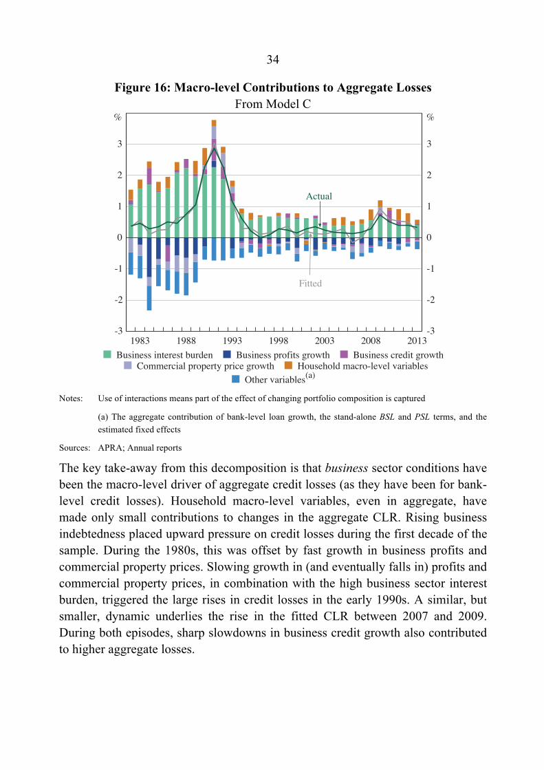
Another way to look at the influence of macro-level variables is to examine the contribution of each variable to the aggregate current loss ratio predicted by Model C. Figure 16 plots the contribution of each macro-level variable and its interacted portfolio share to the CLR of the whole sample in each year.20 The contributions of all household macro-level variables are shown as an aggregate, as are the contributions of the variables in the model that are not interacted with macro-level variables.21 The aggregate level of credit losses predicted by Model C fits actual losses quite closely (the RMSE is 0.15), so this model provides a macro-level explanation that, while suffering from the same limitations as all models, quite closely fits the actual experience.

20 As an example, the contribution of commercial property price growth (CPPG) in 1991 is:

,1990 1 ,1990 1991ˆ

i ii ABSL CPPGω β

∈∑ , where A is the set of banks in the sample in 1991, and ωi,1990 the appropriate weight for each bank (each bank’s share of sample loans, based on loans outstanding in 1990).

21 This is shown as the ‘Other variables’ contribution in Figure 16.

Business creditgrowth (rise)

Commercial propertyprice growth (falls)

Business profitsgrowth (falls)

Business interestrate (rises)

0.0 0.1 0.2 0.3 0.4 0.5Current loss ratio

Higherbusiness

debt

34

Figure 16: Macro-level Contributions to Aggregate Losses From Model C

Notes: Use of interactions means part of the effect of changing portfolio composition is captured

(a) The aggregate contribution of bank-level loan growth, the stand-alone BSL and PSL terms, and the estimated fixed effects

Sources: APRA; Annual reports

The key take-away from this decomposition is that business sector conditions have been the macro-level driver of aggregate credit losses (as they have been for bank-level credit losses). Household macro-level variables, even in aggregate, have made only small contributions to changes in the aggregate CLR. Rising business indebtedness placed upward pressure on credit losses during the first decade of the sample. During the 1980s, this was offset by fast growth in business profits and commercial property prices. Slowing growth in (and eventually falls in) profits and commercial property prices, in combination with the high business sector interest burden, triggered the large rises in credit losses in the early 1990s. A similar, but smaller, dynamic underlies the rise in the fitted CLR between 2007 and 2009. During both episodes, sharp slowdowns in business credit growth also contributed to higher aggregate losses.

1983 1988 1993 1998 2003 2008 2013-3

-2

-1

0

1

2

3

-3

-2

-1

0

1

2

3

Fitted

%%

Actual

Business interest burden Business profits growth Business credit growth Commercial property price growth Household macro-level variables

Other variables(a)

35

By construction, Figure 16 attributes most of the variation in aggregate credit losses to macro-level variables, as it aggregates the contribution of changes in each macro-level variable and changes in the portfolio share with which it is interacted. Figure 17 takes the alternative approach of applying changes in macro-level variables while holding the banking system constant. This is done for two reference years, 1991 and 2008. For example, the line for 1991 shows the aggregate CLR predicted by Model C for the 16 banks in the sample in 1991, applying the actual macro-level variables experienced in each year, but freezing each bank’s portfolio composition and past loan growth at 1991 values. The distance between each of counterfactual lines and the actual fitted values from Model C shows how changes in the banks in the sample, and their characteristics (from the reference year), contribute to aggregate losses.

Figure 17 indicates that different macro-level experiences do not explain all of the difference in credit losses between the early 1990s and global financial crisis episodes. For example, the banking system in 2008, if subjected to the macro-level conditions present in the early 1990s, is predicted to incur credit losses of around 5½ per cent over the period (the area under the 2008 line between 1990 and 1994). This is 3 percentage points below the actual credit loss ratio incurred over this period.22 A reasonable conclusion is that both changes in the macroeconomic environment and changes in the structure of the banking system explain the large difference in credit losses between the early 1990s and global financial crisis episodes.

Caution should be used in giving causal interpretations to the relationships estimated by these econometric models. While most of the estimated relationships are intuitive – the business sector interest burden, for example, has a very natural relationship with credit losses – reverse causality may be present. A good example of this is the United States during the global financial crisis, where credit losses on residential mortgages destabilised large financial intermediaries with consequent impacts upon broader economic and financial conditions (Hall 2010; Mishkin 2011). This causal chain is likely to have been less important in Australia during my sample period, mainly because of the robust position of the Australian

22 An alternative estimate is the area between the 1991 and fitted CLR lines between 2008 and

2012. This is smaller (around ½ percentage point). The large difference between these estimates is an inherent drawback of the structure of Model C.

36

banking system over the whole period (including while it was subject to large credit losses in the early 1990s). This argument is not that there is no casual channel from credit losses to macroeconomic conditions in Australia, but rather that it was not triggered during my sample period. Public actions during crisis periods have also dampened this channel in Australia.

Figure 17: The Contribution of Banking System Structure From Model C

Note: (a) Fitted losses holding banks in the sample and their characteristics at the values in the indicated year

The results of Model C are robust to a number of alternative specifications, including alternative portfolio interactions, alternative lag structures, and different sample periods (see Section C.1 of Appendix C). Omitted variable bias is probably the greatest statistical concern: lending standards have not been discussed in the context of the models, but are likely very important for credit losses.

4.4 Lending Standards

The econometric models above treat all business lending as having equal propensity to cause credit losses (conditional on the macroeconomic environment), regardless of whether it is business lending in the early 1990s or in the mid 2000s, and regardless of the bank doing the lending. But there is evidence that this is not an accurate assumption; that, for example, lending standards were worse in the late

1983 1988 1993 1998 2003 2008 2013-1

0

1

2

3

-1

0

1

2

3

With the banking system in 2008(a)

%%

With the banking system in 1991(a)Fitted currentloss ratio

37

1980s than in the early 2000s. And, internationally, empirical work has shown that lending standards vary over time and played a role in the global financial crisis (see, for example, Lown, Morgan and Rohatgi (2000); Maddaloni and Peydró (2011); and Dell’Ariccia, Igan and Laeven (2012)). This section of the paper attempts to quantitatively explore the effect lending standards have had on credit losses in Australia.

Lending standards, particularly for lending to businesses, are not well-defined in the literature. The definition I employ is given in Section 3.1.1: non-price differences in borrower characteristics and loan terms that are ex ante observable by a bank. Importantly, I do not include portfolio composition at the level of business, housing and personal lending as a component of lending standards. Some examples of changing lending standards were given in Section 3.1.1. But my definition encompasses other differences, such as the industry composition of a bank’s business lending. A business lending portfolio with a higher share of commercial property lending, which has historically been riskier than other business lending (Ellis and Naughtin 2010), could be described as of a lower standard under my definition.

Changes in average lending standards over time are captured reasonably well by Model C, given its close fit at the aggregate level. Several of the macro-level variables in this model likely act as proxies for lending standards. As shown in Figure 15, the long-run relationship between business credit growth and credit losses is positive, and this probably captures increases in credit supply that involve lending to less financially sound borrowers (see, for example, Keeton (1999)). Jiménez and Saurina (2006) use loan-level data to show that, controlling for macroeconomic conditions, loans originated while a bank is growing faster are more likely to default and less likely to be collateralised.

The business sector interest burden is also likely acting as a proxy for average lending standards. Banks extending business loans often place a contractual limit upon businesses’ interest burdens (at origination and/or over time). The aggregate business sector interest burden, the weighted average of the interest burdens of all businesses in the economy, captures some portion of the time series variation in this lending standard. Firm-level data illustrate this clearly. Looking at the largest 300 listed companies at each point in time, firm-level interest burdens were higher in 1990 than in either 1982 or 2008 (Figure 18). For example, around half of the

38

largest 300 listed firms had an interest burden above 50 per cent in 1990, while less than one-fifth of the largest 300 listed firms in 1982 had an interest burden above this level. This variation is partly captured by the aggregate business sector interest burden, which was 17.0, 28.4 and 16.2 in 1982, 1990 and 2008.23 The firm-level ranking also correlates with the relative magnitudes of the credit losses experienced during the downturns that began in each of these years.

Figure 18: Firm-level Interest Burdens CDF for largest 300 listed non-financial firms in each year

Notes: CDF denotes cumulative distribution function; firms with no debt have been excluded; loss-makers with

debt are assigned an interest burden of 120 per cent

Sources: Morningstar; RBA; Statex

In contrast, Model C does a poor job of explaining cross-sectional variation in lending standards. Model residuals during the early 1990s are very large for some state government-owned banks, and the narrative evidence presented in Section 3 indicates that these banks had below-average lending standards (Figure 19). The bank-level variables included in Model C, portfolio composition and bank-level 23 The aggregate and firm-level measures differ slightly. Aggregate interest burden captures

interest on intermediated debt only, while the firm-level measure captures interest on all debt. The aggregate measures of business profits, gross operating surplus (for private non-financial corporates) and gross mixed income (for unincorporated enterprises) differ somewhat from the firm-level measure, earnings before interest and tax.

0.0

0.2

0.4

0.6

0.8

1.0

0 20 40 60 80 100Interest burden (interest expense / EBIT) – %

1990

2008

1982

39

loan growth, do not explain why the credit loss ratios experienced by these banks were so much larger than those at other banks. This omission of lending standards is partly responsible for the higher RMSE of Model C at the bank level: this statistic drops from 63 to 44 basis points if state government-owned banks are excluded.

Figure 19: The Omission of Lending Standards Lines show residuals from Model C for individual banks, as at September

There has almost certainly been more variation in lending standards than is indicated by this state government-owned/non-state government-owned distinction. But little other hard information on lending standards is available. Quantile regression is one strategy that has been used to assess the effect of unobserved heterogeneity in other areas of economics.24 This method models the distribution of credit losses, conditional on the explanatory variables. It provides a more complete description of relationships than least squares regression, which is based upon estimating only the conditional mean of a dependent variable. If unobserved differences in lending standards are the primary determinant of the conditional distribution of credit losses, estimated relationships with macro-level variables at higher (lower) quantiles can be interpreted as being for banks with worse (better) lending standards. If other factors (e.g. idiosyncratic risk) are the primary 24 Bitler, Gelbach and Hoynes (2006), for example, examine quantile treatment effects in a

labour economics context. ‘Quantile’ is a synonym for ‘percentile’.

1986 1988 1990 1992 1994-4

-2

0

2

4

-4

-2

0

2

4

State government-owned banks

Other banks

pptppt

40

determinants of the conditional distribution of credit losses, this interpretation does not hold and quantile regression estimates merely show the range of possible responses to changes in macro-level variables.

Quantile regression is also more robust to outlier observations than least squares methods (Cameron and Trivedi 2009). For example, the significance of commercial property prices in the above models could be driven entirely by a very strong relationship for a subset of banks that experienced credit losses well above-average. But in a quantile regression, this should be apparent in the lack of a relationship between the variables and some parts of the credit losses distribution.

Quantile regression generates estimated relationships with macro-level variables that vary widely across the distribution, and do so in a way that is statistically significant in some cases (Figure 20; full quantile regression outputs are in Table C1).25 Notably, key macro-level variables are estimated to have statistically significant effects, signed in line with estimated coefficients in Model C, on losses across almost all of the distribution. For example, the effect of the business sector interest burden upon losses at the 90th percentile is more than three times as large as at the 10th percentile. More concretely, a one standard deviation rise in business sector interest burden (5.5 percentage points) raises credit losses by 12 basis points at the 10th decile of the distribution, while it raises credit losses by 43 basis points at the 9th decile (for a bank with 40 per cent business lending). The comparable impact from Model C is 30 basis points.

25 I use a parsimonious version of Model C for the quantile regression, and I drop the fixed

effects.

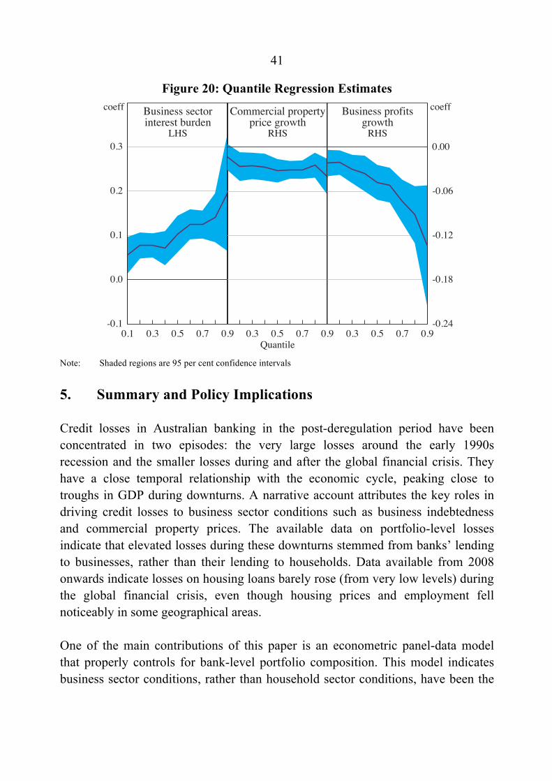
41

Figure 20: Quantile Regression Estimates

Note: Shaded regions are 95 per cent confidence intervals

5. Summary and Policy Implications

Credit losses in Australian banking in the post-deregulation period have been concentrated in two episodes: the very large losses around the early 1990s recession and the smaller losses during and after the global financial crisis. They have a close temporal relationship with the economic cycle, peaking close to troughs in GDP during downturns. A narrative account attributes the key roles in driving credit losses to business sector conditions such as business indebtedness and commercial property prices. The available data on portfolio-level losses indicate that elevated losses during these downturns stemmed from banks’ lending to businesses, rather than their lending to households. Data available from 2008 onwards indicate losses on housing loans barely rose (from very low levels) during the global financial crisis, even though housing prices and employment fell noticeably in some geographical areas.

One of the main contributions of this paper is an econometric panel-data model that properly controls for bank-level portfolio composition. This model indicates business sector conditions, rather than household sector conditions, have been the

0.1 0.3 0.5 0.7 0.9-0.1

0.0

0.1

0.2

0.3

0.3 0.5 0.7 0.9Quantile

0.3 0.5 0.7 0.9-0.24

-0.18

-0.12

-0.06

0.00

coeffBusiness profitsgrowth

RHS

Commercial propertyprice growth

RHS

Business sectorinterest burden

LHS

coeff

42

driver of domestic credit losses over the period studied. The relevant business sector conditions – interest burden, profitability and commercial property prices – are indicators of the ability of this sector to service its debts and of the value of the collateral behind these debts. As a corollary, the model indicates that most losses over the past three decades were incurred on banks’ business lending, and household losses were largely unresponsive to economic conditions in that period. Unlike past work, these results are consistent with the narrative account of credit losses in Australian banking.

Descriptive accounts attribute the scale of losses during the early 1990s to poor lending standards, and the data support this. One piece of evidence, based on quantile regressions, indicates that changes in macro-level conditions have had very different impacts upon banks with similar portfolios (in terms of the shares of business, housing and personal lending). Most compellingly, standard models cannot explain the extremely high credit losses experienced at some state government-owned banks in the early 1990s. Given the anecdotal evidence that these banks had below-average lending standards, this is consistent with the conclusion that poor lending standards have caused the very worst credit loss outcomes over recent decades.

These conclusions have practical implications for stress testing. The credit loss models in this paper that use least squares estimation, and include bank-level variables, are unable to explain, and so unlikely to predict, the very worst credit loss outcomes. Many stress-testing exercises use similar (and in some cases simpler) econometric models (see, for example, IMF (2012)). As the worst credit loss outcomes are the most relevant when stress testing, this suggests that alternative models are needed. Covas, Rump and Zakrajsek (2013) show that a type of quantile regression (quite different to that in this paper) can provide out-of-sample forecasts that encompass the credit losses experienced by the US banking system during the global financial crisis. In an Australian context, Durrani, Peat and Arnold (2014) show that allowing variation in credit risk outcomes across banks, rather than applying the same average risk parameters to all banks, can lead to significantly larger loss estimates.

Stress-testing models could also be improved by incorporating better data on lending standards. The Federal Reserve collects and makes use of loan-level data on borrower characteristics in its annual stress tests of the largest US banks (Board

43

of Governors 2014). This captures some aspects of the risk profile of borrowers; more work is probably needed to make it possible to systemise and accurately record banks’ lending standards.

The historical experience of credit losses at Australian banks this paper describes should help to guide overall understanding of the credit risk they currently face. It supports a continued focus on the analysis of the financial health of the business sector (one output of this work is a chapter of the Reserve Bank’s semiannual Financial Stability Review). As another example, credit loss measures appear to peak before asset performance measures, potentially providing an early signal of future improvement in financial system stability.

The lack of a historical relationship between household sector conditions and credit losses should be used cautiously in contemporary debates on the riskiness of housing lending. It indicates that the macroeconomic shocks experienced by the household sector during the past three decades have been small relative to the lending standards in place for housing lending over this period. Future macroeconomic shocks may, however, have a larger impact on households. There have been, for example, no large nationwide falls in house prices during recent decades. In addition, a rise in unemployment on par with that in the early 1990s could be expected to have a more severe influence on household credit losses, given the large rise in household indebtedness over the intervening period. A corollary of this rise in household indebtedness is the greater share of banks’ lending now made up by housing and personal lending. These considerations suggest that any weakening in lending standards in these areas could have a larger systemic impact than in the past.

44

Appendix A: More Accounting

A.1 Credit Losses

Banks’ financial reports provide a number of different items which capture credit losses:

1. Net charge to profit and loss account for individual provisions: For most loans, when a bank identifies that it has incurred a loss on the loan, it must raise an individual provision (a liability) in order to reduce the carrying value of the loan to the amount it expects to recover. This reduction in net assets is a loss and must be recognised as an expense to the profit and loss account. The net charge incorporates the release of individual provisions held against loans that no longer require them (because, for example, a borrower has recommenced making repayments).

2. Net charge to profit and loss for collective provisions: Similar to 1, but collective provisions are held against incurred losses on loan portfolios with similar characteristics (usually retail loans that are too small to deal with individually), and the losses historical experience suggests are likely on the portfolio of currently healthy loans (to an extent, see Appendix B).

3. Transfers from collective provisions to individual provisions: Some banks fund all provisions through collective provisions at first. When losses on individual loans are identified, appropriate amounts are transferred from collective provisions to individual provisions to cover these losses, and an amount necessary to replenish the collective provision to appropriate levels is charged to the profit and loss though item 2.

4. Write-offs and recoveries to individual provisions: Write-offs are the final step of removing troubled assets from the balance sheet, and, for larger loans, are made after losses have been recognised through individual provisions and recoveries of any collateral made. The troubled loan, individual provision and amount recovered should cancel out so that there is no impact on the profit and loss account at this stage.

45

5. Write-offs and recoveries to collective provisions: Loans that have been collectively provisioned for are written off against collective provisions.

6. Write-offs and recoveries direct to profit and loss: Loans where there is no prospect of recovery can be written off immediately upon evidence of loss emerging. As there are no provisions held against such assets, their write-off has an impact upon the profit and loss account. This category sometimes also captures losses on loans that are not adequately covered by existing provisions.

7. Charge for bad and doubtful debts: The total charge to the profit and loss for credit losses: the sum of 1, 2 and 6. The charge for bad and doubtful debts is the net reduction in the value of a bank’s assets due to credit losses in a given period. It appears in a bank’s profit and loss account and so is a component of the net change in a bank’s capital position over each period.

Unlike the charge for bad and doubtful debts, the other two aggregate measures of credit losses used in this paper, net write-offs and current losses, are not calculated in banks’ financial reports. Net write-offs are the sum of 4, 5 and 6; current losses are the sum of 1, 3, 5 and 6.

A.2 Non-performing Assets

‘Performing’ and ‘non-performing’ are a classifications applied to the assets banks hold at amortised cost (mainly loans and some other credit-type assets). These terms are, in most countries, defined by accounting standards and rules set by banking regulators. In Australia, NPAs include two categories:

• Past-due assets are those where repayment is 90+ days in arrears, but which are covered by sufficient collateral such that no loss is expected (well-secured).

• Impaired assets are those where repayment is 90+ days in arrears or otherwise is doubtful and which are not well-secured.

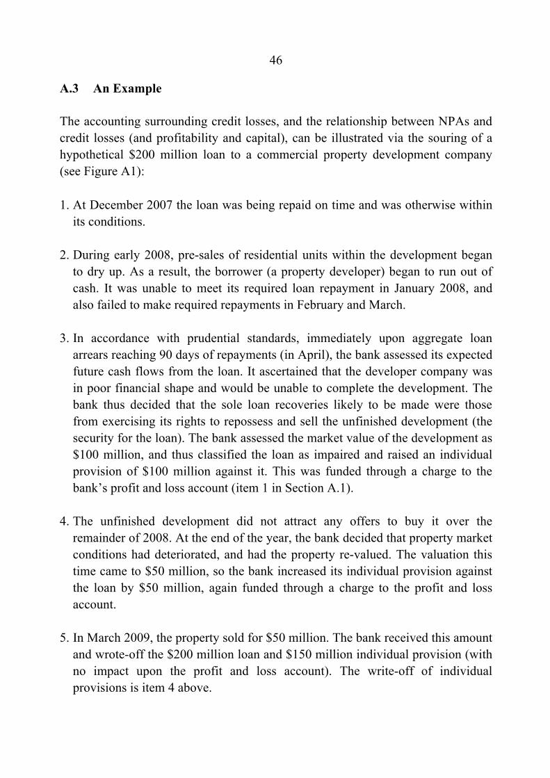
46

A.3 An Example

The accounting surrounding credit losses, and the relationship between NPAs and credit losses (and profitability and capital), can be illustrated via the souring of a hypothetical $200 million loan to a commercial property development company (see Figure A1):

1. At December 2007 the loan was being repaid on time and was otherwise within its conditions.

2. During early 2008, pre-sales of residential units within the development began to dry up. As a result, the borrower (a property developer) began to run out of cash. It was unable to meet its required loan repayment in January 2008, and also failed to make required repayments in February and March.

3. In accordance with prudential standards, immediately upon aggregate loan arrears reaching 90 days of repayments (in April), the bank assessed its expected future cash flows from the loan. It ascertained that the developer company was in poor financial shape and would be unable to complete the development. The bank thus decided that the sole loan recoveries likely to be made were those from exercising its rights to repossess and sell the unfinished development (the security for the loan). The bank assessed the market value of the development as $100 million, and thus classified the loan as impaired and raised an individual provision of $100 million against it. This was funded through a charge to the bank’s profit and loss account (item 1 in Section A.1).

4. The unfinished development did not attract any offers to buy it over the remainder of 2008. At the end of the year, the bank decided that property market conditions had deteriorated, and had the property re-valued. The valuation this time came to $50 million, so the bank increased its individual provision against the loan by $50 million, again funded through a charge to the profit and loss account.

5. In March 2009, the property sold for $50 million. The bank received this amount and wrote-off the $200 million loan and $150 million individual provision (with no impact upon the profit and loss account). The write-off of individual provisions is item 4 above.

47

6. In June 2009, the liquidation of the development company was completed. In the final distribution of assets to its creditors, the bank unexpectedly received $10 million. The bank acknowledged this amount via a recovery direct to profit and loss, which reduced both the cumulative charge for bad and doubtful debts and cumulative net write-offs from the loan to $140 million. This is the net impact on the bank’s profitability and capital of the credit losses caused by the non-repayment of this loan.

Figure A1: Souring of a Hypothetical Loan

This example closely follows how banks have actually dealt with troubled loans over recent years, but there are ways in which the bank could have managed the loan that would have led to different relationships between NPAs and credit losses. For example, the bank could have immediately sold the development for the best available price and written off the necessary amount against its profit and loss account, without ever raising any provisions. Alternatively, the bank could have kept the impaired loan on its books and delayed sale of the development (perhaps for several years) until the market recovered sufficiently to allow a higher sale price. A different asset type could also have changed the relationship: if the asset in question was $200 million worth of residential mortgages, which are normally much better-collateralised, the time profile for NPAs may have been exactly the

100

200

100

200

M J S D M J S D0

100

200

0

100

200

Cumulativenet write-offs

2009

Non-performing assets

$m

$m

$m

$m

Credit losses

Cumulative charge for bad anddoubtful debts/current losses

Individual provisions

Impaired assets

2008

48

same (except made up by past-due, rather than impaired, assets) but credit losses to the bank may have been much lower.

49

Appendix B: Data

B.1 Credit Losses Dataset

The sample of banks for this dataset was selected by obtaining lists of the ten largest banks at each of 1980, 1985, 1990, 1995, 2000, 2005 and 2010, and then attempting to gather data for these banks for the longest possible period. This was not always possible. For example, data were unavailable for many large savings banks during the 1980s, as these were part of banking groups that only published data on their trading bank and consolidated results. The 26 included banks are listed in Table B1. Data for Bankwest, HSBC, and ING from 2002 onwards come for regulatory reports. Major bank time series are split around the incorporation of savings banks in the early 1990s. Time series for other banks are separated around major mergers. For example, Adelaide Bank and Bendigo Bank are separate from the merged Adelaide and Bendigo Bank. The sample includes some observations on banks that are very small in relation to the whole system (less than 1 per cent of total lending). These are excluded from most of the regressions in the paper.

I test for attrition bias in my unbalanced panel in the manner suggested by Wooldridge (2010). I add a dummy variable indicating exit in the next period to Model C. This is insignificant, in the cases in which I define the indicator to capture (i) all attrition from my sample (1 instance through becoming a non-bank asset management company (SBSA), 14 instances through merger, and 5 instances via missing data or falling below the 1 per cent of lending threshold); (ii) just failures and mergers (15 instances); and (iii) the attrition of only SBSA, SBV and Bankwest. These latter three cases are (arguably) the only cases of exit under stress in my sample.

Current loss rates appear to be stationary. The test statistic is less than the 1 per cent critical value in an Im-Pesaran-Shin test of the null hypothesis that credit loss rates are non-stationary. This is also the case in the version of this test that accounts for serial correlation. This result is in line with that of Pain (2003) for UK banks.

50

Table B1: Banks in Sample (continued next page)

Name of bank

Bank type(a)

In sample

Precursor entities

Becomes Banks acquired during sample

period

Alternative names

ANZ (trading) Trading 1980–91 ANZ ANZ Combined 1992–2013 ANZ (trading)

& ANZ (savings)

CBA (trading) Trading 1980–92 CBA Commonwealth Savings Bank

Savings 1980–91 CBA

CBA Combined 1993–2013 CBA (trading) &

Commonwealth Savings Bank

Bankwest (from 2013)

State Bank of NSW (from

2000) State Bank of Victoria (from

1990)

NAB (trading) Trading 1980–92 NAB NAB Combined 1993–2013 NAB (trading)

& NAB (savings)

Westpac (trading)

Trading 1982–93 Westpac

Westpac 1994–2013 Westpac (trading) &

Westpac (savings)

St. George Bank (from 2010)

Bank of Melbourne (from 1998)

St. George Bank

Combined 1989–2009 St. George Building

Society (until 1992)

Advance Bank (from 1997)

State Bank of South Australia

Combined 1985–94

State Bank of NSW

Trading 1981–99 Colonial State (from 1990)

State Bank of Victoria

Savings 1982–90

Bankwest   Combined   1983–2012         Rural and Industries

Bank (prior to 1990)  

51

Table B1: Banks in Sample (continued)

Name   Bank type(a)  

In sample  

Precursor entities  

Becomes   Banks acquired during sample

period  

Alternative names  

Advance Bank Savings 1986–96 Metway Bank Savings 1980–96 Suncorp

Metway Bank

Suncorp Metway Bank

1997–2013 Suncorp Metway Bank

& QIDC

Adelaide Bank 1994–2007 Adelaide and

Bendigo Bank

Bendigo Bank 1994–2007 Adelaide and

Bendigo Bank

Adelaide and Bendigo Bank

2008–13 Adelaide Bank & Bendigo

Bank

Bank of Melbourne

Trading 1989–97

Bank of Queensland

Trading 1980–2013

Deutsche Bank Australia

Trading 1987–92 Changed to branch

status in 1994

Macquarie Bank Trading 1986–2013 ING Bank (Australia)(b)

1995–98, 2002–13

ING Mercantile

Mutual Bank (until 1998)

HSBC Bank Australia(b)

1987–99, 2002–13

Notes: ANZ = Australia and New Zealand Bank; CBA = Commonwealth Bank of Australia; NAB = National Australia Bank; QIDC = Queensland Industry Development Commission; Westpac = Westpac Banking Corporation (a) This column is blank for banks that entered the sample after 1993, given the distinction is not meaningful after this period

(b) Data are not available for the missing years

52

The credit losses of SBSA and SBV have been adjusted to remove the economic impact of support these banks received from their state government owners during the early 1990s. SBV received an indemnity from the Victorian government for losses on a proportion of its loan book. The value of this indemnity has been added to SBV’s credit losses, as it removed the requirement for SBV to raise an equivalent amount of provisions. Direct payments and indemnities given to SBSA have been dealt with in the same way. A large portion of SBSA’s troubled loans were transferred to the state government in 1994 and run-off over the subsequent decade. I have treated this transfer as a write-off by SBSA of these loans and the associated specific provisions.

Changes in accounting standards affect the comparability of credit loss data over time in two main ways. The change from the previous standards to the Australian equivalents to IFRS in the 2006 financial year had an effect on banks’ collective provisions (which were referred to as general provisions before the shift). Compared to the previous standards, IFRS allows less scope for banks to hold provisions against expected future losses. It requires that provisions only be held against losses that have been ‘incurred’, in the sense that they are supported by objective evidence. The five largest banks in Australia reduced their general/collective provisions by around 20 per cent as a result of the change. This outflow from provisions, which was generally absorbed through an increase in shareholders’ equity, has been removed from the charge for bad and doubtful debts in the long-run sample (it does not affect the other two measures of credit losses). Accounting advice and banks’ public statements about their accounting policies indicate that, using various mechanisms, banks continue to raise collective provisions to cover likely future losses under IFRS.

Unlike the previous standards, IFRS requires banks to discount expected future recoveries under impaired loans, at the original interest rate applying to the loan. Thus, upon initial loss recognition, banks must raise higher dollar amounts of provisions. The extra provisions are run down over the period until recovery is made, and this flow is recognised in interest income. The overall effect of the change is that both credit losses and interest income are higher under IFRS than under the previous standards. Some banks provide the amount of the flow to interest income from provisions in their annual reports. Figure B1 presents the aggregate current losses for three banks that publish this data. The average difference between the adjusted and unadjusted ratios is less than 2 basis points.

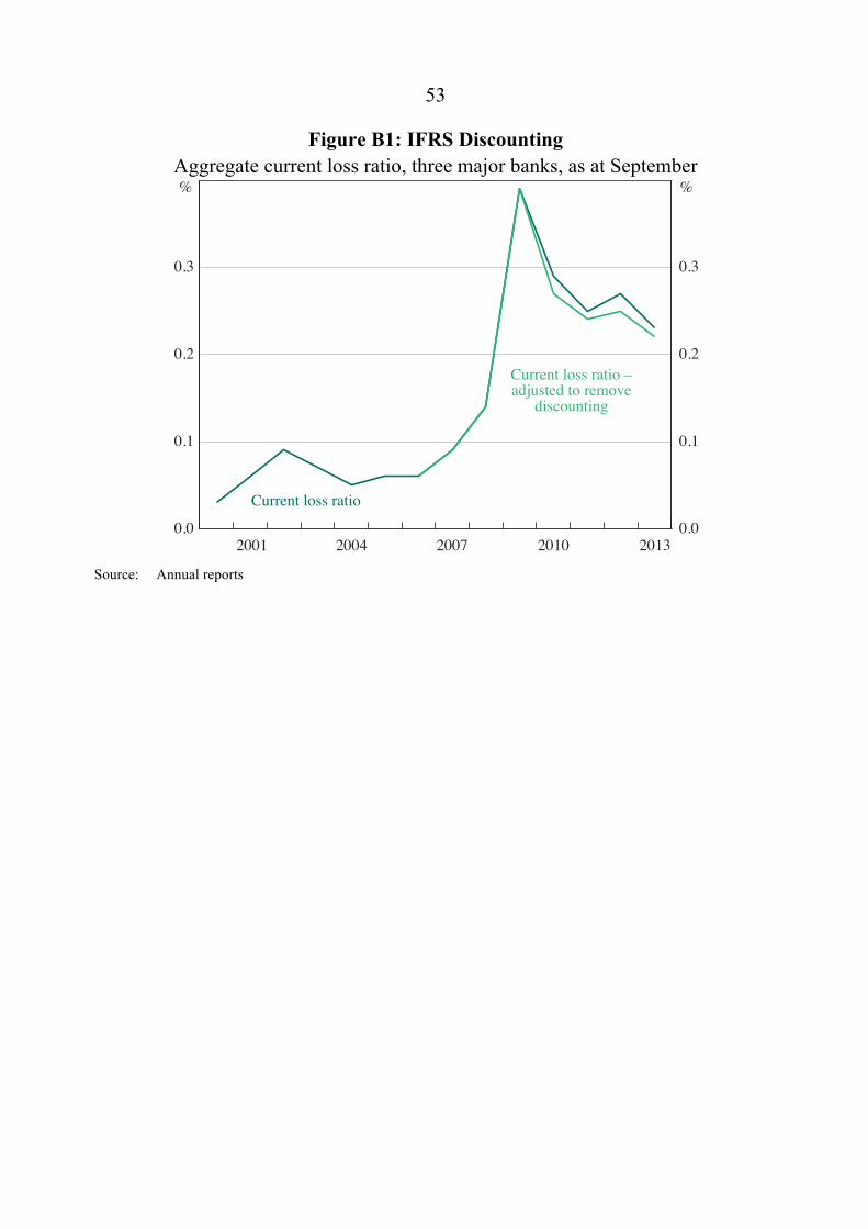
53

Figure B1: IFRS Discounting Aggregate current loss ratio, three major banks, as at September

Source: Annual reports

0.0

0.1

0.2

0.3

0.0

0.1

0.2

0.3

Current loss ratio

2013

%%

2010200720042001

Current loss ratio –adjusted to remove

discounting

54

B.2 Other Data

Table B2: Data Construction and Sources All variables observed at September of each year

Variable Detail Sources Macro-level Real GDP growth Year-on-year growth ABS Cash rate Average over year RBA Economy-wide interest burden (Average intermediated credit outstanding

× average cash rate) / GDP, average over year ABS; APRA; RBA

Inflation Trimmed mean from 1993, average over year ABS; RBA Total credit growth Annual growth APRA; RBA Business sector interest burden (Average intermediated business credit

outstanding × average large business interest rate) / business profits, average over year

ABS; APRA; RBA

Business profits growth Private non-financial corporations’ gross operating surplus + unincorporated enterprises’ gross mixed income, year-on-year growth

ABS

Average interest rate for large businesses

Average over year APRA; RBA

Commercial property price growth

Capital city CBD office property, weighted using ABS shares, annual growth

ABS; JLL Research; RBA

Change in the unemployment rate Annual ABS Household sector interest burden (Average intermediated household credit

outstanding × standard variable mortgage rate) / household disposable income, average over year, year-on-year growth

ABS; APRA; RBA

Household disposable income growth

Before interest payments, year-on-year growth ABS

Standard variable mortgage rate Average over year APRA; RBA Residential property price growth Annual growth REIA Business credit growth Annual growth APRA; RBA Personal credit growth Annual growth APRA; RBA Housing credit growth Annual growth APRA; RBA Bank-level Share of system lending

Business share of lending Share of portfolio that is business lending APRA; RBA Personal share of lending Share of portfolio that is personal lending APRA; RBA Housing share of lending Share of portfolio that is housing lending APRA; RBA

Loan growth Winsorized at the 5th and 95th percentiles APRA; RBA Dummy variable for state government ownership

Author

55

Table B3: Descriptive Statistics

Variable Mean Standard deviation

Minimum Maximum

Macro-level GDP growth 3.22 1.61 –1.91 5.97 Cash rate 8.24 4.41 2.91 17.19 Economy-wide interest burden 9.22 1.87 6.57 13.38 Inflation 4.27 2.99 –0.40 12.40 Total credit growth 11.25 6.23 –0.40 23.99 Business sector interest burden 16.22 5.45 10.01 29.24 Business profits growth 7.43 6.07 –4.62 27.69 Average interest rate for large businesses

10.34 4.55 4.75 20.50

Commercial property price growth 5.95 12.67 –22.81 30.00 Change in the unemployment rate –0.02 1.02 1.61 2.90 Household sector interest burden 7.92 1.94 5.67 12.71 Household disposable income growth

7.77 4.08 1.95 17.50

Standard variable mortgage rate 9.77 3.29 5.80 17.00 Residential property price growth 7.93 8.31 –2.30 41.66 Business credit growth 10.18 9.76 –5.90 30.55 Personal credit growth 8.66 7.38 –5.51 22.32 Housing credit growth 12.91 4.47 4.67 21.58 Bank-level Share of system lending

Business share of lending 0.42 0.23 0.00 0.99 Personal share of lending 0.10 0.09 0.00 0.56 Housing share of lending 0.48 0.28 0.00 1.00

Loan growth 14.47 13.89 –40.53 93.28 Loan growth (winsorized) 14.69 11.34 –0.98 46.27 Dummy variable for state government ownership

0.13 0.34 0.00 1.00

Table B4: Correlations between Macro-level Variables

GD

P gr

owth

Bus

ines

s pro

fits g

row

th

Hou

seho

ld d

ispo

sabl

e in

com

e gr

owth

Com

mer

cial

pro

perty

pric

e gr

owth

Res

iden

tial p

rope

rty p

rice

grow

th

Cas

h ra

te

Ave

rage

inte

rest

rate

for

larg

e bu

sine

sses

Stan

dard

var

iabl

e m

ortg

age

rate

Econ

omy-

wid

e in

tere

st

burd

en

Bus

ines

s sec

tor i

nter

est

burd

en

Hou

seho

ld se

ctor

inte

rest

bu

rden

Tota

l cre

dit g

row

th

Bus

ines

s cre

dit g

row

th

Hou

sing

cre

dit g

row

th

Cha

nge

in th

e un

empl

oym

ent r

ate

Business profits growth 0.61

Household disposable income growth

–0.09 0.17

Commercial property price growth

0.30 0.37 0.57

Residential property price growth

0.24 0.23 –0.07 0.29

Cash rate –0.09 0.14 0.65 0.29 0.02 Average interest rate for large businesses

0.01 0.17 0.58 0.25 0.05 0.97

Standard  variable mortgage rate

–0.03 0.16 0.57 0.24 0.03 0.95 0.96

Economy-wide interest burden –0.27 –0.04 0.05 –0.27 –0.05 0.35 0.29 0.44

56

Business sector interest burden –0.13 0.06 0.08 0.24 0.11 0.68 0.69 0.77 0.68

Household  sector interest burden

–0.25 –0.15 –0.08 –0.18 –0.20 –0.37 –0.46 –0.33 0.58 –0.18

Total credit growth 0.53 0.58 0.55 0.71 0.43 0.54 0.55 0.48 –0.19 0.08 –0.43

Business credit growth 0.42 0.47 0.60 0.74 0.33 0.63 0.60 0.56 0.00 0.16 –0.26 0.94

Housing credit growth 0.49 0.41 0.01 0.08 0.32 0.09 0.20 0.17 –0.32 0.14 –0.55 0.49 0.21

Change in the unemployment rate

–0.86 –0.57 0.15 –0.36 –0.25 0.25 0.15 0.16 0.39 0.29 0.23 –0.43 –0.28 –0.49

Inflation –0.16 0.17 0.75 0.52 0.05 0.82 0.79 0.76 0.09 0.30 –0.32 0.55 0.61 0.01 0.20

57

58

Appendix C: More Regressions

C.1 Robustness

The results of Model C are robust to a number of alternative specifications. In particular:

• The choice to interact business sector variables with the business share of banks’ portfolios is supported statistically. If interactions between the household share of the portfolio and these variables are added to a parsimonious version of Model C (e.g. (PSLi,t – 1 + HSLi,t – 1) × business sector interest burden), they are not significant. Some lending to small businesses in Australia is collateralised by residential property, but an interaction between the business share of lending and residential property price growth is not statistically significant if added to Model C.

• For variables other than credit and loan growth, lagged relationships longer than one year are not a common finding in the literature (see, for example, Hess et al (2009)), and altering the lag structure of Model C changes little. A model with both contemporaneous and lagged values of business profits growth, household disposable income growth, and property prices, leads to very similar estimated coefficients and significance. The only exception to this is that the first lag of household income growth becomes significant at the 5 per cent level. But this variable is only marginally economic significant – a one standard deviation fall in household income raises credit losses by 13 basis points for a representative bank, versus 24 basis points for a one standard deviation fall in business profits.

• Ordinary least squares and random effects models yield coefficient estimates and standard errors very similar to the fixed effects version of Model C in Table 2. The only exception is the importance of the interaction between the personal share of lending and the household sector interest burden. These models estimate a strong and significant (at the 5 per cent level) relationship between the household sector interest burden and losses on personal lending. This result is intuitive, but is not particularly important at the bank level, given the low portfolio share of this type of lending. A one standard deviation increase

59

in this macro-level variable increases credit losses by roughly 5 basis points for a representative bank (with 10 per cent personal lending).

• Economy-wide variables such as GDP growth, changes in the unemployment rate and inflation are insignificant if added to Model C, even if interacted with portfolio shares.

• Several key macro-level variables remain significant if the estimation sample is restricted to a period that excludes the early 1990s downturn. For example, in a model estimated using data for 1997–2013, the business sector interest burden and commercial property prices remain statistically significant and have coefficients similar to Model C, but business profits growth and bank-level loan growth become insignificant.

• A dynamic model including a single lag of current loss ratio was estimated using the Arellano and Bond (1991) estimator. The lagged dependent variable has a positive estimated coefficient and was significant at the 10 per cent level, though unlike for stocks of non-performing assets, there is no strong reason to expect true state dependence over short horizons in the flow of current losses. Estimated coefficients on key explanatory variables in this model were quantitatively similar to Model C. Banks learning from their mistakes may create a negative relationship between credit losses in an earlier downturn and those in a later downturn – something akin to the ‘institutional memory hypothesis’ of Berger and Udell (2004). But only a small number of the banks in the sample during the global financial crisis episode were not present during the early 1990s downturn, so testing this hypothesis is difficult.

• Clustering standard errors two ways – by bank and by year – leads to no substantive change in results. This approach is likely not entirely robust, given the number of clusters in both dimensions is below 50 (Cameron and Miller 2013).

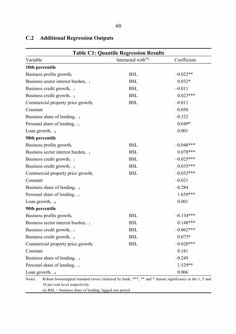
60

C.2 Additional Regression Outputs

Table C1: Quantile Regression Results Variable Interacted with(a): Coefficient 10th percentile Business profits growtht BSL –0.022** Business sector interest burdent – 1 BSL 0.032* Business credit growtht – 1 BSL –0.011 Business credit growtht – 3 BSL 0.023*** Commercial property price growtht BSL –0.011 Constant –0.050 Business share of lendingt – 1 –0.332 Personal share of lendingt – 1 0.649* Loan growtht – 4 0.001 50th percentile Business profits growtht BSL –0.048*** Business sector interest burdent – 1 BSL 0.078*** Business credit growtht – 1 BSL –0.025*** Business credit growtht – 3 BSL 0.035*** Commercial property price growtht BSL –0.032*** Constant –0.021 Business share of lendingt – 1 –0.284 Personal share of lendingt – 1 1.659*** Loan growtht – 4 0.001 90th percentile Business profits growtht BSL –0.134*** Business sector interest burdent – 1 BSL 0.148*** Business credit growtht – 1 BSL –0.062*** Business credit growtht – 3 BSL 0.075* Commercial property price growtht BSL –0.028*** Constant 0.181 Business share of lendingt – 1 –0.249 Personal share of lendingt – 1 1.529** Loan growtht – 4 0.006 Notes: Robust bootstrapped standard errors clustered by bank; ***, ** and * denote significance at the 1, 5 and

10 per cent level respectively (a) BSL = business share of lending; lagged one period

61

References

APRA (Australian Prudential Regulation Authority) (1999), ‘Submission to the Basel Committee on Banking Supervision, Credit Risk Modelling: Current Practices and Applications’, Response to the Basel Committee’s Report Credit Risk Modelling: Current Practices and Applications. Available at <http://apra.gov.au/adi/Documents/Credit-Risk-Modelling-Current-Practices-and-Applications-October-1999.pdf>.

Arellano M and S Bond (1991), ‘Some Tests of Specification for Panel Data: Monte Carlo Evidence and an Application to Employment Equations’, The Review of Economic Studies, 58(2), pp 277–297.

Battellino R and N McMillan (1989), ‘Changes in the Behaviour of Banks and Their Implications for Financial Aggregates’, RBA Research Discussion Paper No 8904.

Berger AN and GF Udell (2004), ‘The Institutional Memory Hypothesis and the Procyclicality of Bank Lending Behavior’, Journal of Financial Intermediation, 13(4), pp 458–495.

Bernanke BS (2010), ‘Causes of the Recent Financial and Economic Crisis’, Statement before the Financial Crisis Inquiry Commission ‘Too Big to Fail: Expectations and Impact of Extraordinary Government Intervention and the Role of Systemic Risk in the Financial Crisis’, Washington DC, 2 September.

Bitler MP, JB Gelbach and HW Hoynes (2006), ‘What Mean Impacts Miss: Distributional Effects of Welfare Reform Experiments’, The American Economic Review, 96(4), pp 988–1012.

Board of Governors (Board of Governors of the Federal Reserve System) (2014), ‘Comprehensive Capital Analysis and Review 2014: Assessment Framework and Results’, Report, March.

Cameron AC and DL Miller (2013), ‘A Practitioner’s Guide to Cluster-Robust Inference’, Unpublished manuscript, University of California – Davis, October.

62

Cameron AC and PK Trivedi (2009), Microeconometrics Using Stata, Stata Press, College Station, Texas.

Carew E (1997), Westpac: The Bank that Broke the Bank, Doubleday, Sydney.

Conroy F (1997), ‘Discussion on “Managing Credit Risk – An Overview”’, in B Gray and C Cassidy (eds), Credit Risk in Banking, Proceedings of a Conference, Reserve Bank of Australia, Sydney, pp 21–23.

Covas FB, B Rump and E Zakrajsek (2013), ‘Stress-Testing U.S. Bank Holding Companies: A Dynamic Panel Quantile Regression Approach’, Board of Governors of the Federal Reserve System Finance and Economics Discussion Series No 2013-55.

Davis EP and H Zhu (2009), ‘Commercial Property Prices and Bank Performance’, The Quarterly Review of Economics and Finance, 49(4), pp 1341–1359.

Dell’Ariccia G, D Igan and L Laeven (2012), ‘Credit Booms and Lending Standards: Evidence from the Subprime Mortgage Market’, Journal of Money, Credit and Banking, 44(2-3), pp 367–384.

Durrani K, M Peat and B Arnold (2014), ‘Stress-Testing Bank Residential Mortgage Portfolios by Decomposing the Mean’, Paper presented at the 12th INFINITI Conference on International Finance ‘Global Finance – Integration or Mere Convergence’, Prato, 9–10 June.

Eales R (1997), ‘Credit Risk Measurement in Corporate Banking – Theory and Practice’, in B Gray and C Cassidy (eds), Credit Risk in Banking, Proceedings of a Conference, Reserve Bank of Australia, Sydney, pp 50–68.

Ellis L and C Naughtin (2010), ‘Commercial Property and Financial Stability – An International Perspective’, RBA Bulletin, June, pp 25–30.

Esho N and A Liaw (2002), ‘Should the Capital Requirement on Housing Lending be Reduced? Evidence from Australian Banks’, Australian Prudential Regulation Authority Working Paper 2002-02.

63

Fitz-Gibbon B and M Gizycki (2001), ‘A History of Last-Resort Lending and Other Support for Troubled Financial Institutions in Australia’, RBA Research Discussion Paper No 2001-07.

Foos D, L Norden and M Weber (2010), ‘Loan Growth and Riskiness of Banks’, Journal of Banking & Finance, 34(12), pp 2929–2940.

Fraser BW (1994), ‘Foreign Banks in Australia’, RBA Bulletin, September, pp 16–22.

Gerlach S, W Peng and C Shu (2005), ‘Macroeconomic Conditions and Banking Performance in Hong Kong SAR: A Panel Data Study’, in Investigating the Relationship between the Financial and Real Economy, BIS Papers No 22, Bank for International Settlements, Basel, pp 481–497.

Gizycki M (2001), ‘The Effect of Macroeconomic Conditions on Banks’ Risk and Profitability’, RBA Research Discussion Paper No 2001-06.

Gizycki M and P Lowe (2000), ‘The Australian Financial System in the 1990s’, in D Gruen and S Shrestha (eds), The Australian Economy in the 1990s, Proceedings of a Conference, Reserve Bank of Australia, Sydney, pp 180–215.

Głogowski A (2008), ‘Macroeconomic Determinants of Polish Banks’ Loan Losses – Results of a Panel Data Study’, National Bank of Poland Working Paper No 53.

Gray B (1998), ‘Credit Risk in the Australian Banking Sector’, Federal Reserve Bank of New York Economic Policy Review, 4(3), pp 61–70.

Hall RE (2010), ‘Why Does the Economy Fall to Pieces after a Financial Crisis?’, The Journal of Economic Perspectives, 24(4), pp 3–20.

Hess K, A Grimes and M Holmes (2009), ‘Credit Losses in Australasian Banking’, The Economic Record, 85(270), pp 331–343.

64

Hoggarth G, A Logan and L Zicchino (2005), ‘Macro Stress Tests of UK Banks’, in Investigating the Relationship between the Financial and Real Economy, BIS Papers No 22, Bank for International Settlements, Basel, pp 392–408.

IMF (International Monetary Fund) (2012), ‘Australia: Financial System Stability Assessment’, IMF Country Report No 12/308.

Jiménez G and J Saurina (2006), ‘Credit Cycles, Credit Risk, and Prudential Regulation’, International Journal of Central Banking, June, pp 65–98.

Keeton WR (1999), ‘Does Faster Loan Growth Lead to Higher Loan Losses?’, Federal Reserve Bank of Kansas City Economic Review, Second Quarter, pp 57–75.

Kent C and P Scott (1991), ‘The Direction of Australian Investment from 1985/86 to 1988/89’, RBA Research Discussion Paper No 9106.

Laker J (2007), ‘The Evolution of Risk and Risk Management – A Prudential Regulator’s Perspective’, in C Kent and J Lawson (eds), The Structure and Resilience of the Financial System, Proceedings of a Conference, Reserve Bank of Australia, Sydney, pp 300–317.

Lee G (1991), ‘The Evaluation and Rating of Banks’, in Proceedings of the 3rd Australian Institute of Bankers Banking and Finance Conference: Melbourne, Victoria July 1 - 2 1991, Australian Institute of Bankers, Melbourne, pp 90–118.

Louzis DP, AT Vouldis and VL Metaxas (2012), ‘Macroeconomic and Bank-Specific Determinants of Non-Performing Loans in Greece: A Comparative Study of Mortgage, Business and Consumer Loan Portfolios’, Journal of Banking & Finance, 36(4), pp 1012–1027.

Lown CS, DP Morgan and S Rohatgi (2000), ‘Listening to Loan Officers: The Impact of Commercial Credit Standards on Lending and Output’, Federal Reserve Bank of New York Economic Policy Review, 6(2), pp 1–16.

65

Macfarlane I (1991), ‘The Lessons for Monetary Policy’, in I Macfarlane (ed), The Deregulation of Financial Intermediaries, Proceedings of a Conference, Reserve Bank of Australia, Sydney, pp 175–199.

MacPherson KI (1993), Report of the Auditor-General on an Investigation into the State Bank of South Australia: Pursuant to Section 25 of the State Bank of South Australia Act 1983 (Amended), Volume 1: Report Pursuant to Terms of Appointment and the State Bank Act, Auditor-General’s Department, Adelaide.

Maddaloni A and J-L Peydró (2011), ‘Bank Risk-Taking, Securitization, Supervision, and Low Interest Rates: Evidence from the Euro-Area and the U.S. Lending Standards’, The Review of Financial Studies, 24(6), pp 2121–2165.

Mishkin FS (2011), ‘Over the Cliff: From the Subprime to the Global Financial Crisis’, The Journal of Economic Perspectives, 25(1), pp 49–70.

Pain D (2003), ‘The Provisioning Experience of the Major UK Banks: A Small Panel Investigation’, Bank of England Working Paper No 177.

Phelps LJ (1989), ‘The Risk Profile of Australian Banks’, Paper presented at the Conference ‘Damage Control: Credit Risk Management for Banks and Financial Institutions’, Organised by Australian Investment Conferences, Sydney, 4–5 September.

RBA (Reserve Bank of Australia) (2010), ‘The Australian Financial System’, in Financial Stability Review, March, pp 17–37.

Salas V and J Saurina (2002), ‘Credit Risk in Two Institutional Regimes: Spanish Commercial and Savings Banks’, Journal of Financial Services Research, 22(3), pp 203–224.

Sykes T (1994), The Bold Riders: Behind Australia’s Corporate Collapses, Allen & Unwin, Sydney.

Ullmer M (1997), ‘Managing Credit Risk – An Overview’, in B Gray and C Cassidy (eds), Credit Risk in Banking, Proceedings of a Conference, Reserve Bank of Australia, Sydney, pp 5–20.

66

Victoria (Victoria. Royal Commission into the Tricontinental Group of Companies) (1991), First Report of the Royal Commission into the Tricontinental Group of Companies, Parliamentary Paper 1988-92 No 172, L.V. North, Government Printer, Melbourne.

von Westernhagen N, E Harada, T Nagata, B Vale, Juan Ayuso, J Saurina, S Daltung, S Ziegler, E Kent, J Reidhill and S Peristiani (2004), ‘Bank Failures in Mature Economies’, Basel Committee on Banking Supervision Working Paper No 13.

Wooldridge JM (2010), Econometric Analysis of Cross Section and Panel Data, 2nd edn, MIT Press, Cambridge.