RESEARCH CENTER - peer.berkeley.edu

PACIFIC EARTHQUAKE ENGINEERING RESEARCH CENTER

Global Collapse of Frame Structures under Seismic Excitations

Luis F. Ibarra

and

Helmut Krawinkler

Stanford University

PEER 2005/06SEPT. 2005

Global Collapse of Frame Structures under Seismic Excitations

Luis F. Ibarra

and

Helmut Krawinkler

John A. Blume Earthquake Engineering Center Department of Civil & Environmental Engineering

Stanford University

PEER Report 2005/06 Pacific Earthquake Engineering Research Center

College of Engineering University of California, Berkeley

September 2005

iii

ABSTRACT

Global collapse in earthquake engineering refers to the inability of a structural system to sustain

gravity loads when subjected to seismic excitation. The research described in this report proposes

a methodology for evaluating global incremental (side-sway) collapse based on a relative

intensity measure instead of an engineering demand parameter (EDP). The relative intensity is

the ratio of ground motion intensity to a structural strength parameter, which is increased until

the response of the system becomes unstable. At this stage the relative intensity – EDP curve

becomes flat (zero slope). The largest relative intensity is referred to as “collapse capacity.”

In order to implement the methodology, deteriorating hysteretic models are developed to

represent the monotonic and cyclic behavior of structural components. Parameter studies that

utilize these deteriorating models are performed to obtain collapse capacities and quantify the

effects of system parameters that most influence collapse for SDOF and MDOF systems. The

dispersion of the collapse capacity due to record to record variability and uncertainty in the

system parameters is evaluated. The latter source of dispersion is quantified by means of the

first-order second-moment method. The studies reveal that softening of the post-yield stiffness in

the backbone curve (post-capping stiffness) and the displacement at which this softening

commences (defined by the ductility capacity) are the two system parameters that most influence

the collapse capacity of a system. Cyclic deterioration is an important but not dominant issue for

collapse evaluation. P-delta effects greatly accelerate the collapse of deteriorating systems and

may be the primary source of collapse for flexible but very ductile structural systems.

The report presents applications of the proposed collapse methodology to the

development of collapse fragility curves and the evaluation of the mean annual frequency of

collapse.

An important contribution is the development of a transparent methodology for the

evaluation of incremental collapse in which the assessment of collapse is closely related to the

physical phenomena that lead to this limit state. The methodology addresses the fact that collapse

is caused by deterioration in complex assemblies of structural components that should be

modeled explicitly.

iv

ACKNOWLEDGMENTS

This work was supported in part by the Pacific Earthquake Engineering Research Center through

the Earthquake Engineering Research Centers Program of the National Science Foundation

under award number EEC-9701568. The work reported herein is part of the PEER mission to

develop and disseminate technologies to support performance-based earthquake engineering.

Any opinions, findings, and conclusions or recommendations expressed in this material

are those of the author(s) and do not necessarily reflect those of the National Science Foundation.

This report was originally published as the Ph.D. dissertation of the first author. The

financial support provided by PEER is gratefully acknowledged. The authors would like to thank

Professors C. A. Cornell, Gregory G. Deierlein, and Eduardo Miranda, who provided

constructive feedback on the manuscript. Several graduate students, present and former, at the

Stanford University John A. Blume Earthquake Engineering Center have provided assistance and

valuable input. In particular, the help provided by Ricardo Medina, Ashraf Ayoub, Curtis

Haselton, Francisco Parisi, Fatheme Jalayer, Dimitrios Vamvatsikos, Jack Baker, Jorge Ruiz-

Garcia, Christoph Adam, Farzin Zareian, and Rohit Kaul is much appreciated.

v

CONTENTS

ABSTRACT.................................................................................................................................. iii

ACKNOWLEDGMENTS ........................................................................................................... iv

CONTENTS....................................................................................................................................v

LIST OF FIGURES ..................................................................................................................... xi

LIST OF TABLES .....................................................................................................................xxv

1 INTRODUCTION .................................................................................................................1

1.1 Motivation for This Study...............................................................................................1

1.2 Objective .........................................................................................................................2

1.3 Outline.............................................................................................................................2

2 COLLAPSE METHODOLOGY .........................................................................................5

2.1 Introduction.....................................................................................................................5

2.2 Previous Research on Global Collapse ...........................................................................5

2.3 Description of Global Collapse Assessment Approach ................................................10

2.3.1 Selection of Ground Motions ............................................................................11

2.3.2 Deterioration Models ........................................................................................11

2.3.3 Structural Systems.............................................................................................12

2.3.4 Collapse Capacity .............................................................................................12

2.3.5 Effect of Deterioration Prior to Collapse ..........................................................15

2.3.6 Effects of Uncertainty in System Parameters....................................................16

2.3.7 Collapse Fragility Curves and Mean Annual Frequency of Collapse...............16

2.3.8 Statistical Considerations ..................................................................................17

2.3.9 Normalization....................................................................................................18

3 HYSTERETIC MODELS...................................................................................................29

3.1 Introduction...................................................................................................................29

3.2 Basic Hysteretic Models ...............................................................................................30

3.2.1 Description of Backbone Curve ........................................................................30

3.2.2 Bilinear Model ..................................................................................................31

3.2.3 Peak-Oriented Model ........................................................................................31

3.2.4 Pinching Model .................................................................................................32

vi

3.3 Cyclic Deterioration......................................................................................................32

3.3.1 Deterioration Based on Hysteretic Energy Dissipation ....................................32

3.3.2 Basic Strength Deterioration .............................................................................33

3.3.3 Post-Capping Strength Deterioration ................................................................34

3.3.4 Unloading Stiffness Deterioration ....................................................................35

3.3.5 Accelerated Reloading Stiffness Deterioration.................................................36

3.4 Calibration of Hysteretic Models with Component Tests.............................................36

3.4.1 Steel Specimens ................................................................................................37

3.4.2 Wood Specimens...............................................................................................38

3.4.3 Reinforced Concrete Specimens .......................................................................39

3.5 Illustrations of Cyclic Deterioration Effects .................................................................39

3.6 Additional Observations on Deterioration Model.........................................................40

3.7 Summary .......................................................................................................................42

4 COLLAPSE ASSESSMENT OF SDOF SYSTEMS ........................................................53

4.1 Introduction...................................................................................................................53

4.2 Systems and Ground Motions Considered in Parameter Study ....................................54

4.2.1 Parameters Evaluated in Primary Parameter Study ..........................................55

4.2.2 Parameters Evaluated in Secondary Parameter Study ......................................57

4.2.3 Set of Ground Motion Records LMSR-N .........................................................58

4.3 Results of Primary Parameter Study .............................................................................59

4.3.1 Effect of Deterioration on EDPs Prior to Collapse ...........................................60

4.3.2 General Trends in Collapse Capacity Spectra, (Sa,c/g)/η - T ............................61

4.3.3 Effect of Post-Capping Stiffness on Collapse Capacity....................................62

4.3.4 Effect of Ductility Capacity on Collapse Capacity ...........................................64

4.3.5 Effect of Cyclic Deterioration on Collapse Capacity........................................65

4.3.6 Effect of P-∆ on Collapse Capacity ..................................................................66

4.3.7 Effect of Type of Hysteretic Model on Collapse Capacity ...............................69

4.3.8 Increment in Collapse Capacity after Cap Displacement, δc, is Reached .........70

4.4 Results of Secondary Parameter Analysis ....................................................................71

4.4.1 Effect of Residual Strength, λFy, on Collapse Capacity ...................................71

4.4.2 Effect of Individual Cyclic Deterioration Modes..............................................73

vii

4.4.3 Effect of Level of Pinching in Pinched Hysteretic Model, κf,d .........................76

4.4.4 Effect of Damping Formulation ........................................................................76

4.4.5 Effect of Numerical Value of ξο .......................................................................79

4.4.6 Deteriorating SDOF Systems Subjected to Near-Fault Ground Motions .........80

4.4.7 Deteriorating SDOF Systems Subjected to Long-Duration Ground

Motions .............................................................................................................82

4.5 Summary .......................................................................................................................84

4.5.1 Results of Primary Parameter Study .................................................................84

4.5.2 Results of Secondary Parameter Study .............................................................86

5 GLOBAL COLLAPSE OF MDOF SYSTEMS..............................................................131

5.1 Introduction.................................................................................................................131

5.2 Collapse Capacity of MDOF Systems ........................................................................132

5.3 MDOF Systems Used for Collapse Evaluation...........................................................133

5.3.1 Basic Characteristics of Generic Frames ........................................................133

5.3.2 Deteriorating Characteristics of Plastic Hinge Springs of Generic Frames....135

5.3.3 Set of Ground Motions....................................................................................136

5.4 EDPs for Generic Frames with Infinitely Strong Columns ........................................136

5.4.1 Effect of Deterioration Parameters on EDPs ..................................................136

5.4.2 Global Pushover Curves for Deteriorating Systems .......................................138

5.4.3 De-Normalized EDPs......................................................................................141

5.5 Collapse Capacity of Generic Frames with Infinitely Strong Columns......................142

5.5.1 Collapse Capacity for the Set of Reference Frames........................................142

5.5.2 Effect of Post-Capping Stiffness on Collapse Capacity..................................143

5.5.3 Effect of Ductility Capacity on Collapse Capacity .........................................143

5.5.4 Effect of Cyclic Deterioration on Collapse Capacity......................................144

5.5.5 Effect of Hysteretic Models on Collapse Capacity .........................................144

5.5.6 Effect of P-∆ Effects on Collapse Capacity ....................................................145

5.6 Results for Generic Frames with Columns of Finite Strength ....................................146

5.7 Equivalent SDOF Systems Including P-∆ Effects ......................................................148

5.7.1 Equivalent SDOF Systems without Consideration of P-∆ Effects..................149

viii

5.7.2 Auxiliary Backbone Curve and Stability Coefficient to Include

P-∆ Effects .....................................................................................................149

5.7.3 Procedure to Obtain Collapse Capacity of MDOF Structures Based on

Collapse Capacity of Equivalent SDOF Systems ...........................................152

5.7.4 Illustration of Procedure to Obtain Collapse Capacity of MDOF

Structures Based on Collapse Capacity of Equivalent SDOF Systems ..........153

5.8 Summary .....................................................................................................................155

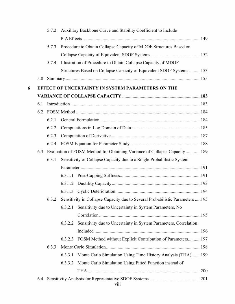
6 EFFECT OF UNCERTAINTY IN SYSTEM PARAMETERS ON THE

VARIANCE OF COLLAPSE CAPACITY ....................................................................183

6.1 Introduction.................................................................................................................183

6.2 FOSM Method ............................................................................................................184

6.2.1 General Formulation .......................................................................................184

6.2.2 Computations in Log Domain of Data ............................................................185

6.2.3 Computation of Derivative..............................................................................187

6.2.4 FOSM Equation for Parameter Study .............................................................188

6.3 Evaluation of FOSM Method for Obtaining Variance of Collapse Capacity .............189

6.3.1 Sensitivity of Collapse Capacity due to a Single Probabilistic System

Parameter ........................................................................................................191

6.3.1.1 Post-Capping Stiffness......................................................................191

6.3.1.2 Ductility Capacity.............................................................................193

6.3.1.3 Cyclic Deterioration..........................................................................194

6.3.2 Sensitivity in Collapse Capacity due to Several Probabilistic Parameters .....195

6.3.2.1 Sensitivity due to Uncertainty in System Parameters, No

Correlation ........................................................................................195

6.3.2.2 Sensitivity due to Uncertainty in System Parameters, Correlation

Included ............................................................................................196

6.3.2.3 FOSM Method without Explicit Contribution of Parameters...........197

6.3.3 Monte Carlo Simulation..................................................................................198

6.3.3.1 Monte Carlo Simulation Using Time History Analysis (THA)........199

6.3.3.2 Monte Carlo Simulation Using Fitted Function instead of

THA ..................................................................................................200

6.4 Sensitivity Analysis for Representative SDOF Systems.............................................201

ix

6.5 Sensitivity Computation for MDOF Systems Using FOSM Method .........................204

6.6 Summary .....................................................................................................................205

7 FRAGILITY CURVES AND MEAN ANNUAL FREQUENCY OF COLLAPSE.....233

7.1 Introduction.................................................................................................................233

7.2 Collapse Fragility Curves (FCs)..................................................................................233

7.2.1 Normalized Counted Collapse Fragility Curves .............................................234

7.2.2 Normalized Collapse Fragility Curves Obtained by Fitting Log-Normal

Distribution to Data.........................................................................................235

7.2.3 De-Normalization of Collapse Fragility Curves .............................................236

7.2.4 Collapse Fragility Curves for MDOF Frames with Parameter Variations......237

7.3 Spectral Acceleration Hazard......................................................................................238

7.4 Mean Annual Frequency of Global Collapse..............................................................239

7.4.1 Formulation.....................................................................................................239

7.4.2 Computation of Mean Annual Frequency of Collapse for a Specific Site,

SDOF Systems ................................................................................................241

7.4.3 Computation of Mean Annual Frequency of Collapse for a Specific Site,

MDOF Systems...............................................................................................242

7.5 Summary .....................................................................................................................243

8 SUMMARY AND CONCLUSIONS................................................................................259

REFERENCES...........................................................................................................................269

APPENDIX A: “COUNTED” AND “COMPUTED” STATISTICAL VALUES..............279

A.1 “Computed” Statistical Values....................................................................................279

A.2 “Counted” Statistical Values.......................................................................................280

APPENDIX B: PROPERTIES OF GENERIC FRAME MODELS...................................283

B.1 Modal and Structural Properties of the Generic Frames.............................................283

B.2 Stiffness of Rotational Springs at Member Ends ........................................................284

B.3 Parameters for Deteriorating Springs..........................................................................286

B.4 Modeling of Plastic Hinges to Avoid Spurious Damping Moments .........................288

APPENDIX C: PROBABILITY DISTRIBUTION OF COLLAPSE CAPACITY...........291

C.1 Lognormal Distribution Paper and Kolmogorov-Smirnov Goodness-of-Fit Test .....291

C.2 Collapse Capacity Distribution due to RTR Variability ............................................292

x

C.3 Summary ....................................................................................................................293

APPENDIX D: COMPUTATIONS OF VARIANCE OF COLLAPSE CAPACITY IN

THE LINEAR DOMAIN OF THE DATA .................................................295

D.1 Formulation for Computations of Collapse Capacity in Linear Domain....................295

D.2 Linear Domain and Log Domain of Data ...................................................................296

D.2.1 Multiplicative versus Additive Approach .......................................................296

D.2.2 Computations in Linear and Log Domain of Data..........................................297

D.3 Summary .....................................................................................................................298

xi

LIST OF FIGURES

Figure 2.1 Relative intensity–EDP curve ..................................................................................20

Figure 2.2 SDOF response of a peak-oriented model with rapid cyclic deterioration ..............20

Figure 2.3 Backbone curves for different η values (constant Sa/g) ...........................................21

Figure 2.4 (Sa/g)/η - δmax/Sd curves............................................................................................21

Figure 2.5 Variation of collapse capacity with period...............................................................22

Figure 2.6 Median (Sa/g)/η - δmax/δy curves, different δc/δy values ...........................................22

Figure 2.7 Representation of uncertainty in system parameters................................................23

Figure 2.8 Contribution of uncertainty in system parameters to variance of (Sa,c/g)/η ............23

Figure 2.9 Examples of fragility curves for SDOF systems with T = 0.5 s...............................24

Figure 2.10 Assessment of mean annual frequency of collapse ..................................................24

Figure 2.11 Period and strength dependence of mean annual frequency of collapse for

ductile SDOF systems (Van Nuys location) ............................................................25

Figure 2.12 IDA curves for an intermediate ductile SDOF system, η = 0.1 ...............................26

Figure 2.13 Strength variation curves for an intermediate ductile SDOF system, Sa/g = 0.5 .....26

Figure 2.14 NEHRP design spectrum for soil type D, L.A. site..................................................27

Figure 2.15 Median strength associated with collapse for an intermediate ductile system,

Sa(T)/g according to NEHRP design spectrum ........................................................27

Figure 3.1 Experimental hysteretic loops for a wood specimen subjected to monotonic and

cyclic loading. ..........................................................................................................43

Figure 3.2 Backbone curve for hysteretic models .....................................................................43

Figure 3.3 Bilinear hysteretic model with strength limit ...........................................................43

Figure 3.4 Peak-oriented hysteretic model; (a) basic model rules, (b) Mahin and Bertero’s

modification (Mahin and Bertero, 1975)..................................................................44

Figure 3.5 Pinching hysteretic model; (a) basic model rules, (b) reloading deformation at

the right of break point ............................................................................................44

Figure 3.6 Peak-oriented model with individual deterioration modes ......................................45

Figure 3.7 Calibration of bilinear model on steel component tests using the SAC

standard loading protocol (Uang et al., 2000) ..........................................................46

xii

Figure 3.8 Calibration of bilinear model on steel component tests using the SAC

near-fault protocol (Uang et al., 2000) .....................................................................46

Figure 3.9 History of NHE dissipation, SAC standard loading protocol test of Fig. 3.7,

bilinear model...........................................................................................................46

Figure 3.10 History of NHE dissipation, SAC near-fault loading protocol tests of Fig. 3.8,

bilinear model...........................................................................................................47

Figure 3.11 Calibration of pinching model on plywood shear-wall component tests

(Gatto and Uang, 2002) ............................................................................................47

Figure 3.12 History of NHE dissipation, pinching model and loading protocols for tests of

Fig. 3.11....................................................................................................................48

Figure 3.13 Calibration of pinching model on reinforced concrete columns of Moehle and

Sezen experiments (Sezen, 2000).............................................................................48

Figure 3.14 History of NHE dissipation, pinching model and tests of Fig. 3.13 ........................49

Figure 3.15 CUREE standard loading protocol ...........................................................................49

Figure 3.16 Deterioration effect on hysteretic response; peak-oriented model, CUREE

protocol, αs = 0.03, αc = -0.10 .................................................................................50

Figure 3.17 Deterioration effect on hysteretic response; peak-oriented model, CUREE

protocol, αs = 0.03, αc = -0.50 .................................................................................51

Figure 4.1 Backbone curves for hysteretic models with and without P-∆.................................91

Figure 4.2 Spectra of ordinary GMs scaled to the same Sa at T = 0.9 s.....................................91

Figure 4.3 Effect of CD on EDPs; T = 0.9 s, αc = -0.1, δc/δy = 4, P-∆= 0.................................92

Figure 4.4 Effect of CD on δmax/δy; T = 0.2 s, αc = -0.1, δc/δy = 4, P-∆= 0 ...............................92

Figure 4.5 Effect of CD on δmax/δy; T = 3.6 s; αc = -0.1, δc/δy = 4, P-∆= 0 ...............................93

Figure 4.6 Effect of αc on δmax/δy; T = 0.9 s, δc/δy = 4, γ = inf., P-∆= 0 ....................................93

Figure 4.7 Effect of αc on median δmax/δy; T = 0.2 and 3.6 s, δc/δy = 4, γ = inf., P-∆= 0 ..........93

Figure 4.8 Effect of δc/δy on EDPs; T = 0.9 s, αc = -0.1, γ = inf., P-∆= 0..................................94

Figure 4.9 Effect of δc/δy on EDP ratios; T = 0.2 and 3.6 s, αc = -0.1, γ = inf., P-∆= 0 ............94

Figure 4.10 Set of median collapse capacity spectra for peak-oriented models..........................94

Figure 4.11 Collapse capacity spectra for selected peak-oriented models ..................................95

Figure 4.12 Dependence of median (Sa,c/g)/η on αc; δc/δy = 4, slow CD, T = 0.1 s–1.0 . ...........95

Figure 4.13 Effect of αc on (Sa,c/g)/η; δc/δy = 4, no CD, no P-∆ .................................................96

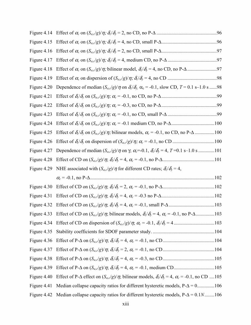
xiii

Figure 4.14 Effect of αc on (Sa,c/g)/η; δc/δy = 2, no CD, no P-∆ .................................................96

Figure 4.15 Effect of αc on (Sa,c/g)/η; δc/δy = 4, no CD, small P-∆.............................................96

Figure 4.16 Effect of αc on (Sa,c/g)/η; δc/δy = 2, no CD, small P-∆.............................................97

Figure 4.17 Effect of αc on (Sa,c/g)/η; δc/δy = 4, medium CD, no P-∆ ........................................97

Figure 4.18 Effect of αc on (Sa,c/g)/η; bilinear model, δc/δy = 4, no CD, no P-∆ ........................97

Figure 4.19 Effect of αc on dispersion of (Sa,c/g)/η; δc/δy = 4, no CD ........................................98

Figure 4.20 Dependence of median (Sa,c/g)/η on δc/δy; αc = -0.1, slow CD, T = 0.1 s–1.0 s ......98

Figure 4.21 Effect of δc/δy on (Sa,c/g)/η; αc = -0.1, no CD, no P-∆ .............................................99

Figure 4.22 Effect of δc/δy on (Sa,c/g)/η; αc = -0.3, no CD, no P-∆ .............................................99

Figure 4.23 Effect of δc/δy on (Sa,c/g)/η; αc = -0.1, no CD, small P-∆ ........................................99

Figure 4.24 Effect of δc/δy on (Sa,c/g)/η; αc = -0.1 medium CD, no P-∆ ...................................100

Figure 4.25 Effect of δc/δy on (Sa,c/g)/η; bilinear models, αc = -0.1, no CD, no P-∆ ................100

Figure 4.26 Effect of δc/δy on dispersion of (Sa,c/g)/η; αc = -0.1, no CD ..................................100

Figure 4.27 Dependence of median (Sa,c/g)/η on γ; αc=-0.1, δc/δy = 4, T =0.1 s–1.0 s .............101

Figure 4.28 Effect of CD on (Sa,c/g)/η; δc/δy = 4, αc = -0.1, no P-∆..........................................101

Figure 4.29 NHE associated with (Sa,c/g)/η for different CD rates; δc/δy = 4,

αc = -0.1, no P-∆.....................................................................................................102

Figure 4.30 Effect of CD on (Sa,c/g)/η; δc/δy = 2, αc = -0.1, no P-∆..........................................102

Figure 4.31 Effect of CD on (Sa,c/g)/η; δc/δy = 4, αc = -0.3 no P-∆...........................................102

Figure 4.32 Effect of CD on (Sa,c/g)/η; δc/δy = 4, αc = -0.1, small P-∆ .....................................103

Figure 4.33 Effect of CD on (Sa,c/g)/η; bilinear models, δc/δy = 4, αc = -0.1, no P-∆ ...............103

Figure 4.34 Effect of CD on dispersion of (Sa,c/g)/η; αc = -0.1, δc/δy = 4 .................................103

Figure 4.35 Stability coefficients for SDOF parameter study. ..................................................104

Figure 4.36 Effect of P-∆ on (Sa,c/g)/η; δc/δy = 4, αc = -0.1, no CD..........................................104



Figure 4.39 Effect of P-∆ on (Sa,c/g)/η; δc/δy = 4, αc = -0.1, medium CD.................................105

Figure 4.40 Effect of P-∆ effect on (Sa,c/g)/η; bilinear models, δc/δy = 4, αc = -0.1, no CD ....105

Figure 4.41 Median collapse capacity ratios for different hysteretic models, P-∆ = 0..............106

Figure 4.42 Median collapse capacity ratios for different hysteretic models, P-∆ = 0.1N ........106

xiv

Figure 4.43 Examples of collapse capacity ratios for bilinear / peak-oriented hysteretic

models ...................................................................................................................106

Figure 4.44 Effect of hysteretic model on median collapse capacity; systems with different

δc/δy and αc values ..................................................................................................107

Figure 4.45 Effect of hysteretic model on median collapse capacity; systems with different

CD rates..................................................................................................................107

Figure 4.46 Median ratios of (Sa,c/g)/η over (Sa/g)/η when δ = δc; P-∆ =0...............................108

Figure 4.47 Median ratios of (Sa,c/g)/η over (Sa/g)/η when δ = δc, P-∆ =0.1N. ........................109

Figure 4.48 Median ratios of (Sa,c/g)/η over (Sa/g)/η when δ = δc; different P-∆ levels ...........109

Figure 4.49 Hysteretic response for a system with residual strength .......................................110

Figure 4.50 Normalized collapse displacements (δf /δy) for systems with residual strength .....111

Figure 4.51 Effect of residual strength on (Sa,c/g)/η for ductile systems...................................111

Figure 4.52 Effect of residual strength on (Sa,c/g)/η for non-ductile systems ...........................111

Figure 4.53 Effect of residual strength on (Sa,c/g)/η for ductile systems with CD....................112

Figure 4.54 Effect of residual strength on (Sa,c/g)/η for non-ductile systems with CD.............112

Figure 4.55 δmax/δy at collapse for a ductile system...................................................................112

Figure 4.56 δmax/δy at collapse for a ductile system when δf (λ>0) ≤ 1.6 δf (λ=0) .....................113

Figure 4.57 Effect of residual strength on collapse displacements considering

δf (λ>0) ≤ 1.6 δf (λ=0).............................................................................................113

Figure 4.58 Effect of cyclic basic strength deterioration on the hysteretic response of

systems without strength capping ..........................................................................114

Figure 4.59 Effect of cyclic basic strength deterioration on (Sa,C/G)/η, systems without

strength capping .....................................................................................................114

Figure 4.60 Effect of cyclic basic strength deterioration on the hysteretic response of

systems with strength capping................................................................................115

Figure 4.61 Effect of cyclic basic strength deterioration on (Sa,c/g)/η ......................................115

Figure 4.62 Effect of cyclic post-capping strength deterioration on the hysteretic response....116

Figure 4.63 Effect of cyclic post-capping strength deterioration on (Sa,c/g)/η..........................116

Figure 4.64 Effect of cyclic unloading stiffness deterioration on the hysteretic response of

a system with strength capping ..............................................................................117

Figure 4.65 Effect of cyclic unloading stiffness deterioration on (Sa,c/g)/η ..............................117

xv

Figure 4.66 Effect of cyclic reloading accelerated stiffness deterioration on the hysteretic

response of a system with strength capping ..........................................................118

Figure 4.67 Effect of cyclic accelerated stiffness deterioration on (Sa,c/g)/η ............................118

Figure 4.68 Effect of pinching level on (Sa,c/g)/η for ductile systems ......................................119

Figure 4.69 Effect of pinching level on (Sa,c/g)/η for non-ductile systems ...............................119

Figure 4.70 Damping ratio–frequency relationship ..................................................................120

Figure 4.71 Effect of damping formulation on δmax/Sd for non-deteriorating systems,

T = 0.5 s, ξο = 5%...................................................................................................120

Figure 4.72 Effect of damping formulation on median δmax/Sd ratios, non-deteriorating

systems, ξ = 5% .....................................................................................................120

Figure 4.73 Effect of damping formulation on (Sa,c/g)/η, P-∆ = 0, ξο = 5% .............................121

Figure 4.74 Effect of damping formulation on (Sa,c/g)/η, small P-∆, ξο = 5%..........................121

Figure 4.75 Effect of damping formulation on (Sa,c/g)/η , P-∆ = 0, ξο = 10% ..........................121

Figure 4.76 Effect of damping formulation on (Sa,c/g)/η, small P-∆, ξο = 10% .......................122

Figure 4.77 Effect of ξο on (Sa,c/g)/η, mass proportional damping ..........................................122

Figure 4.78 Effect of ξο on (Sa,c/g)/η, stiffness proportional damping .....................................122

Figure 4.79 Velocity time history of a typical NFGM ..............................................................123

Figure 4.80 Pulse P2 ground acceleration time history (Babak and Krawinkler, 2001) ..........123

Figure 4.81 Elastic strength (acceleration) demand spectrum for Pulse P2 ..............................123

Figure 4.82 Elastic strength demand spectra of NFGMs and Pulse P2, scaled at

Sa(T/Tp) = 0.8..........................................................................................................124

Figure 4.83 Collapse capacities for systems w/o CD subjected to Set NF-11 and Pulse P2.....125

Figure 4.84 Collapse capacities for systems with rapid CD subjected to Set nf-11 and

Pulse P2 ..................................................................................................................125

Figure 4.85 Dispersion of collapse capacities for systems subjected to Set NF-11 ..................126

Figure 4.86 Effect of CD on (Sa,c/g)/η for systems subjected to Set NF-11 and Pulse P2 .......126

Figure 4.87 Effect of CD on (Sa,c/g)/η for systems subjected to Set NF-11; δc/δy = 4,

αc = -0.10 ...............................................................................................................127

Figure 4.88 Effect of CD on (Sa,c/g)/η for systems subjected to Set NF-11; δc/δy = 4,

αc = -0.30 ...............................................................................................................127

Figure 4.89 Median elastic spectra for Sets LD-13 and LMSR-N ............................................128

xvi

Figure 4.90 NHE at collapse for reference SDOF system; slow CD for sets LD-13 and

LMSR-N ................................................................................................................128

Figure 4.91 Ratios of NHE at collapse for reference SDOF system with different CD rates,

Sets LD-13 over LMSR-N .....................................................................................129

Figure 4.92 Effect of CD on (Sa,c/g)/η for systems subjected to sets of GM with different

strong motion duration ...........................................................................................129

Figure 4.93 Effect of CD on median collapse capacity ratios for systems subjected to sets of

GM with different strong motion duration.............................................................130

Figure 4.94 Effect of CD on median collapse capacity ratios for systems subjected to sets

of GM with strong motion duration, bilinear models.............................................130

Figure 5.1 Family of generic frames, stiff and flexible frames (after Medina, 2002) .............159

Figure 5.2 Beam hinge (BH) mechanism ................................................................................159

Figure 5.3 Individual and statistical [Sa(T1)/g]/γ - EDP relationships for set of reference

frame 0918 and statistical relationships for set of non-deteriorating frames ........160

Figure 5.4 Median normalized maximum story drift profiles for a 9-story frame with

T1 = 1.8 s.................................................................................................................161

Figure 5.5 Effect of αc of rotational springs on maximum of story drift over story yield

drift over the height, 9-story frames with T1 = 1.8 s.. ............................................162

Figure 5.6 Effect of δc/δy of rotational springs on maximum of story drift over story

yield drift over the height, 9-story frames with T1 = 1.8 s .....................................162

Figure 5.7 Effect of CD rate of rotational springs on maximum of story drift over story

yield drift over the height, 9-story frames with T1 = 1.8 s. ....................................163

Figure 5.8 Global pushover curves for the non-deteriorating and deteriorating (reference)

frame 0909..............................................................................................................163

Figure 5.9 Deflected shapes from pushover analyses for non-deteriorating 18-story frames

(after Medina, 2002)...............................................................................................164

Figure 5.10 Deflected shapes from pushover analyses for frame 0909.....................................164

Figure 5.11 Moment-rotation relationships of rotational springs at beam ends and

columns base, reference frame 0909 ......................................................................165

Figure 5.12 Moment (*1/1000) vs. normalized roof drift of columns and beams of reference

frame 0909..............................................................................................................166

xvii

Figure 5.13 Maximum roof drift angle from dynamic and static nonlinear analysis for the

3-story reference frames.........................................................................................167

Figure 5.14 Maximum roof drift angle from dynamic and static nonlinear analysis for the

9-story reference frames.........................................................................................167

Figure 5.15 Ratio of maximum interstory drift angle over maximum roof drift angle, 3 and

9-story-reference frames ........................................................................................167

Figure 5.16 Median and 16th percentile collapse capacity spectra, set of reference frames......168

Figure 5.17 Median collapse capacities — number of stories, set of reference frames. ...........168

Figure 5.18 Effect of αc of springs on collapse capacity of generic frames, δc/δy = 4,

γs,c,k,a = inf. ..............................................................................................................169

Figure 5.19 Effect of δc/δy of springs on collapse capacity of generic frames, αc = -0.1,

γs,c,k,a = inf. ..............................................................................................................170

Figure 5.20 Effect of δc/δy of springs on collapse capacity of generic frames, αc = -0.3,

γs,c,k,a = inf. ..............................................................................................................171

Figure 5.21 Effect of CD of springs on collapse capacity of generic frames, δc/δy = 4,

αc = -0.1..................................................................................................................172

Figure 5.22 Effect of hysteretic model on median collapse capacity of generic frames ...........173

Figure 5.23 Elastic and inelastic stability coefficients obtained from global pushover

curves, peak-oriented non-deteriorating frame 1836. ............................................173

Figure 5.24 Post-yield stiffness ratio and stability coefficients from global pushover curves,

generic frames with strain hardening in rotational springs of 3%..........................174

Figure 5.25 Collapse capacity of flexible non-deteriorating and flexible reference frames

with P-∆ effects ......................................................................................................175

Figure 5.26 Effect of P-∆ on collapse capacity of reference frames .........................................175

Figure 5.27 Effect of P-∆ on global pushover curves for reference frame 1212.......................176

Figure 5.28 Maximum strong-column factor over the height for reference frame 0909...........177

Figure 5.29 Effect on median collapse capacity of including columns with high strength

( pbc MM ,4.2∑ = ) ..................................................................................................177

Figure 5.30 Effect on median collapse capacity of including columns with intermediate

strength ( pbc MM ,2.1∑ = ).....................................................................................178

xviii

Figure 5.31 Effect on median collapse capacity of including columns with low strength

( pbc MM ,0.1∑ = ) ..................................................................................................178

Figure 5.32 Representation of P-D effects in SDOF systems ...................................................179

Figure 5.33 P-∆ Effects obtained with an auxiliary backbone curve based on elastic and

inelastic stability coefficients .................................................................................180

Figure 5.34 P-∆ effects obtained with a simplified auxiliary backbone curve and rotation

of the strain-hardening branch by the inelastic stability coefficient ......................180

Figure 5.35 Collapse capacities for equivalent SDOF systems using different P-∆

approaches..............................................................................................................181

Figure 5.36 Collapse capacity–inelastic stability coefficient curves obtained from SDOF

systems with auxiliary backbone Curves, T0 = 3.6 s. .............................................181

Figure 5.37 Test of collapse capacity–inelastic stability coefficient curves for MDOF

structures with t0 = 3.6 s. and variations of αs at the rotational springs.................182

Figure 5.38 Test of collapse capacity–inelastic stability coefficient curves for MDOF

structures with T0 = 3.6 s and variations of P/W ratio............................................182

Figure 6.1 Approximations of derivative xxg ∂∂ /)( for computing 2)(ln , XS ca

σ using the

FOSM method ........................................................................................................208

Figure 6.2 Collapse capacity spectra for different αc values; δc/δy = 4, slow CD ...................208

Figure 6.3 Dependence of median (Sa,c/g)/η on αc in the linear domain of the data;

δc/δy = 4, slow CD ..................................................................................................209

Figure 6.4 Dependence of median (Sa,c/g)/η on αc in the log domain of the data; δc/δy = 4,

slow CD..................................................................................................................209

Figure 6.5 2)(ln , ασ

caS and 2)(ln , RTRS ca

σ for reference SDOF system1. derivative based on

)exp( ln1 αµ=x and )exp( lnln2 αα σµ +=x .....................................................................210

Figure 6.6 Effect on 2)(ln

2)(ln ,,/ RTRSS cacaσσ α of the increment used for computing the

derivative, reference SDOF system, )exp( ln1 αµ=x and )exp( lnln2 αα σµ nx += ........210

1 Section 6.2.4 contains the definitions of contributions to variance of collapse capacity such as 2

)(ln , ασcaS

xix



derivative; reference system, )exp( lnln1 αα σµ nx −= and )exp( lnln2 αα σµ nx += ........211

Figure 6.8 Effect of the assumed ασ ln on 2)(ln

2)(ln ,,/ RTRSS cacaσσ α ratios; reference SDOF

system, derivatives based on )exp( lnln1 αα σµ −=x and )exp( lnln2 αα σµ +=x ............211

Figure 6.9 Collapse capacity spectra for different (δc/δy –1); αc = -0.10, slow CD ................212

Figure 6.10 Dependence of median (Sa,c/g)/η on δc/δy; αc = -0.10, slow CD, periods from

T = 0.1–1.0 s. ..........................................................................................................212


2)(ln ,,/ RTRSS cacaσσ δ of the increment used for computing the

derivative. reference system, )exp( lnln1 δδ σµ nx −= and )exp( lnln2 δδ σµ nx += ........213

Figure 6.12 Effect of the selected δσ ln on 2)(ln

2)(ln ,,/ RTRSS cacaσσ δ ratios; reference SDOF

system, derivatives based on )exp( lnln1 δδ σµ −=x and )exp( lnln2 δδ σµ +=x .............213

Figure 6.13 Collapse capacity spectra for different CD rates; δc/δy = 4, αc = -0.10..................214

Figure 6.14 Dependence of median (Sa,c/g)/η on γs,c,k,a; αc = -0.10, δc/δy= 4, periods from

T = 0.1–1.0 s. ..........................................................................................................214


2)(ln ,,/ RTRSS cacaσσ γ of the increment used for computing the

derivative; reference system, )exp( lnln1 γγ σµ nx −= and )exp( lnln2 γγ σµ nx += ........215

Figure 6.16 Effect of the selected γσ ln on 2)(ln

2)(ln ,,/ RTRSS cacaσσ γ ratios; reference SDOF

system, derivatives based on )exp( lnln1 γγ σµ −=x and )exp( lnln2 γγ σµ +=x .............215

Figure 6.17 2)(ln

2)(ln ,,/ RTRSXS caicaσσ ratios for different system parameters; derivatives with

)exp( lnln1 xxx σµ −= and )exp( lnln2 xxx σµ += , reference system...............................216

Figure 6.18 Contribution of uncertainty in system parameters to 2)(ln , TOTS ca

σ ; reference

system, no correlation included..............................................................................216


σ ; reference

system, low correlation included............................................................................217

Figure 6.20 Contribution of ij correlation to combined correlation, 5.0, =jiρ ........................217

xx


σ ; reference

system, high correlation included...........................................................................218

Figure 6.22 2)(ln , RTRS ca

σ , 2)(ln , XS ca

σ and 2)(ln , TOTS ca

σ ; reference system, full correlation................218

Figure 6.23 Comparison of 2)(ln , TOTS ca

σ obtained with FOSM method by considering explicit

and non-explicit contribution of system parameters, full correlation ....................219

Figure 6.24 Dependence of median (Sa,c/g)/η on αc; Monte Carlo simulation with

uncertainty in αc and in the three probabilistic system parameters, T = 0.6 s........219

Figure 6.25 Dependence of median (Sa,c/g)/η on δc/δy; Monte Carlo simulation with

uncertainty in δc/δy and in the three probabilistic system parameters, T = 0.6 s ....220

Figure 6.26 Dependence of median (Sa,c/g)/η on γs,c,k,a; Monte Carlo simulation with

uncertainty in γs,c,k,a and in the three probabilistic system parameters, T = 0.6 s ...220

Figure 6.27 Comparison of fragility curves obtained from counted and fitted lognormal

distributions of 2)(ln , ασ

caS .........................................................................................221

Figure 6.28 Fragility curves from fitted lognormal distributions for 2)(ln , ασ

caS and 2)(ln , XS ca

σ ....221

Figure 6.29 Comparison of 2)(ln , ica XSσ obtained with FOSM (solid lines) and Monte Carlo

simulation; reference system, full correlation ........................................................222

Figure 6.30 Regression for dependence of (Sa,c/g)/η on αc at T = 0.5 s, reference SDOF

system.....................................................................................................................222

Figure 6.31 Histogram of 2)(ln , ασ

caS from Monte Carlo simulation; reference SDOF system,

T = 0.5 s..................................................................................................................223

Figure 6.32 Comparison of 2)(ln

2)(ln ,,/ RTRSS cacaσσ α ratios for FOSM method and approximation

from linear regression, reference SDOF system ....................................................223

Figure 6.33 Contributions to variance of (Sa,c/g)/η for a peak-oriented system with

intermediate ductility, no P-∆.................................................................................224


δc/δy = 4, αc = -0.30, γs,c,k,a = 50, no P-∆ effects.....................................................225

Figure 6.35 Contributions to variance of (Sa,c/g)/η for a peak-oriented system with low

ductility, no P-∆......................................................................................................226

xxi

Figure 6.36 Contributions to variance of (Sa,c/g)/η for a peak-oriented system with high

ductility, no P-∆......................................................................................................226

Figure 6.37 Contributions to variance of (Sa,c/g)/η for a bilinear system with intermediate

ductility, no P-∆......................................................................................................226


intermediate ductility, small P-∆ ............................................................................227


δc/δy = 4, αc = -0.30, γs,c,k,a = 50, small P-∆............................................................227

Figure 6.40 Contributions to variance of (Sa,c/g)/η for a peak-oriented system with low

ductility small P-∆ ..................................................................................................227

Figure 6.41 Contributions to variance of (Sa,c/g)/η for a peak-oriented system with high

ductility, small P-∆ .................................................................................................228

Figure 6.42 Contributions to variance of (Sa,c/g)/η for a bilinear system with intermediate

ductility, small P-∆ .................................................................................................228

Figure 6.43 Contributions to 2)(ln , TOTS ca

σ for set of MDOF systems with T = 0.1N and

springs at ends of beams with intermediate ductile characteristics........................229

Figure 6.44 i,j correlation/combined correlation for set of MDOF systems with T = 0.1N

and springs at ends of beams with intermediate ductile characteristics .................229


σ , 2)(ln , XS ca


σ for set of MDOF systems with T = 0.1N


Figure 6.46 Contributions to 2)(ln , TOTS ca

σ for set of MDOF systems with T = 0.2N and

springs at ends of beams with intermediate ductile characteristics........................230

Figure 6.47 i,j correlation/combined correlation for set of MDOF systems with T = 0.2N



σ , 2)(ln , XS ca


σ for set of MDOF systems with T = 0.2N


Figure 7.1 Counted fragility curves for SDOF systems ..........................................................245

Figure 7.2 Fragility curves for SDOF systems obtained by fitting a lognormal

distribution ............................................................................................................246

xxii

Figure 7.3 Collapse capacity ratios for different probabilities of collapse, T = 0.5 s .............247

Figure 7.4 De-normalization of fragility curves at different base shear strength for SDOF

systems; baseline hysteretic properties, T = 0.6 s ..................................................247

Figure 7.5 Fragility curves for frame structures with springs at beam ends with baseline

hysteretic properties ...............................................................................................248

Figure 7.6 Fragility curves for stiff generic frames of 3 and 9-stories with parameter

variations in springs of the beams ..........................................................................249

Figure 7.7 Fragility curves for 18-story generic frames with parameter variations in the

springs of the beams...............................................................................................250

Figure 7.8 Equal hazard spectra used to derive hazard curves for specific periods ................251

Figure 7.9 Hazard curves obtained from linear regression analysis by using 50/50, 10/50

and 2/50 seismic hazard levels, T = 0.5 s ...............................................................251

Figure 7.10 Hazard curves obtained from linear regression analysis by using 50/50, 10/50

and 2/50 seismic hazard levels, T = 0.5, 1.0 and 2.0 s ...........................................252

Figure 7.11 Fragility curves of SDOF systems with baseline hysteretic properties for

computing MAF of collapse, η = 0.2 .....................................................................252

Figure 7.12 HC, FC, and MAF of collapse due to xSa = at T = 0.5 s.; SDOF system with

baseline hysteretic properties, η = 0.2....................................................................253

Figure 7.13 Mean annual frequency of collapse due to xSa = for SDOF systems with

baseline hysteretic properties, η = 0.2....................................................................253

Figure 7.14 Mean annual frequency of collapse for SDOF systems with baseline

hysteretic properties for different η’s and periods .................................................254

Figure 7.15 Mean annual frequency of collapse for SDOF systems with different

hysteretic properties, η = 0.2..................................................................................254

Figure 7.16 MAF of collapse for SDOF systems with dispersion due to RTR variability plus

uncertainty in the system par.; αc=-0.1, δc/δy=4, γs,c,k,a= 50 ...................................255

Figure 7.17 MAF of collapse for deterministic SDOF systems, systems with dispersion due

to RTR variability, and systems with dispersion due to RTR variability

plus uncertainty in the system PAR., αc=-0.1, δc/δy=4, γs,c,k,a= 50.........................255

Figure 7.18 Fragility curves of stiff generic frames with baseline hysteretic properties in the

springs of the beams, γ = 0.2 ..................................................................................256

xxiii

Figure 7.19 Mean annual frequency of collapse for stiff generic frames; baseline hysteretic

properties in the springs of the beams, different γ’s...............................................256

Figure 7.20 Fragility curves of flexible generic frames with baseline hysteretic properties in

the springs of the beams, γ = 0.2 ...........................................................................257

Figure 7.21 Mean annual frequency of collapse for flexible generic frames, baseline

hysteretic properties in the springs of the beams, different γ’s. .............................257

Figure 7.22 Comparison of mean annual frequency of collapse for flexible and stiff frames,

baseline hysteretic properties in the springs of the beams, different. γ’s ...............258

Figure B.1 Moment-rotation relationship for a member based on the moment-rotation of

the plastic hinge springs and elastic beam-column element .................................290

Figure C.1 Fitting of lognormal distribution to collapse capacity data; peak-oriented

SDOF systems, dispersion due to RTR variability ...............................................294

Figure C.2 Fitting of lognormal distribution to collapse capacity data; generic frames with

T1 = 0.6 s; springs with intermediate ductility .......................................................294

Figure D.1 Standard deviation of collapse capacity under variations of αc .............................299

Figure D.2 Coefficient of variation of collapse capacity under variations of αc......................299

Figure D.3 Effect of the domain of the computations on 2)(

2)( ,,/ RTRSS cacaσσ α and

2)(ln

2)(ln ,,/ RTRSS cacaσσ α ratios; derivatives with αc at 16th and 84th of each domain ...300

Figure D.4 16th and 84th percentiles for computing the derivative on the linear and log

domain of the data ..................................................................................................300

Figure D.5 Effect of the domain of the computations on 2)(


2)(ln

2)(ln ,,/ RTRSS cacaσσ α ratios; derivatives with th

αln16 and thαln84 for both domains ....301

Figure D.6 2)(ln

2)(ln ,,/ RTRSS cacaσσ α ratios for computations in the log domain of the data;

derivatives with αc at thαln16 and th

αln84 and at thα16 and th

α84 ...................................301

xxv

LIST OF TABLES

Table 4.1 SDOF systems of primary parameter study, peak-oriented models, P-∆=0.............88

Table 4.2 Set of ordinary ground motion records, LMSR-N (after Medina, 2002) .................89

Table 4.3 Set of near-fault ground motions, NF-11 .................................................................89

Table 4.4 Set of long-duration records, LD-13 ........................................................................90

Table 5.1 Parameters of springs of sets of generic frames used for collapse evaluation .......158

Table B.1 Modal properties, N = 9, T1 = 0.9 and 1.8 s. ..........................................................289

Table B.2 Structural properties, N = 9, T1 = 0.9 s. ..................................................................289

Table B.3 Structural properties, N = 9, T1 = 1.8 s. ..................................................................289

1 Introduction

1.1 1.1 MOTIVATION FOR THIS STUDY

Protection against collapse has always been a major objective of seismic design. In earthquake

engineering, collapse refers to a structural system’s loss of capacity to resist gravity loads when

subjected to seismic excitation. Global collapse may imply dynamic instability in a side-sway

mode, usually triggered by large story drifts, which are amplified by P-∆ effects and

deterioration in strength and stiffness of the components of the system.

Assessment of collapse safety necessitates the capability to predict the dynamic response

of deteriorating systems, particularly for existing older construction in which deterioration

commences at relatively small deformations. Because of the lack of hysteretic models capable of

simulating deteriorating behavior, global collapse is usually assumed to be associated with an

“acceptable” story drift or the attainment of a limit value of deformation in individual

components of the structure. This approach does not permit a “redistribution” of damage and

does not account for the capacity of the system before collapse to sustain deformations that are

significantly larger than those associated with loss in the resistance of individual elements.

Thus, a systematic approach to integrate all the sources of global collapse needs to be

developed. The approach should include the effect of backbone strength deterioration, cyclic

deterioration, (CD), and P-∆ effects on the global collapse of structural systems. In the context

of this report, global collapse implies incremental “side-sway” collapse of at least one story of

the structure.

1.2 1.2 OBJECTIVE

The main objective of the study is to develop a methodology for evaluating global (side-sway)

collapse for deteriorating structural systems. The evaluation of collapse is based on a measure

called the “relative intensity,” which is defined as the ratio of the ground motion intensity to a

2

structural strength parameter. The relative intensity at collapse is called “collapse capacity.” The

components of this methodology are:

• Development of hysteresis models that incorporate all important phenomena contributing

to global collapse;

• Computation of the collapse capacity for representative sets of frame structures and

ground motions;

• Evaluation of statistical measures of the collapse capacity, and of the effect of

uncertainties in ground motions and in structural parameters on these statistical measures;

• Development of collapse fragility curves; and

• Evaluation of the mean annual frequency of collapse.

1.3 1.3 OUTLINE

The general methodology for assessing side-sway collapse is described in Chapter 2, where the

main concepts used in this investigation are introduced and advantages and limitations of the

procedure are illustrated. A literature review of the most salient findings in the evaluation of

structural collapse is also included.

Chapter 3 focuses on the development of deteriorating component hysteretic models,

including strength deterioration of the backbone curve and cyclic deterioration of strength and

stiffness. The calibration of the hysteretic models with experimental results is illustrated. The

models are implemented in an in-house single-degree-of-freedom (SDOF) program that carries

out dynamic and quasi-static inelastic analysis, and in a dynamic nonlinear analysis program for

multi-degree-of-freedom (MDOF) systems.

Collapse evaluation of SDOF systems is the topic of Chapter 4. A parametric study is

carried out to determine the main parameters that influence collapse, such as type of hysteretic

model, ductility capacity, and post-capping stiffness. Statistics for collapse capacity are

computed considering record-to-record (RTR) variability.

Chapter 5 deals with global collapse of generic frames whose inelastic behavior is

modeled by springs at the ends of structural members. Initially, collapse capacity is obtained for

strong column–weak beam frames, considering columns with infinite strength. Later, the “strong

column–weak beam” concept is tested by adjusting the strength of the columns to specific strong

3

column factors. A procedure for obtaining equivalent SDOF systems for deteriorating MDOF

systems including P-∆ effects is also presented.

In Chapter 6 the sensitivity of collapse capacity to uncertainty in the system parameters is

investigated by using the first-order second-moment method (FOSM). Different alternatives for

applying the FOSM method to the evaluation of collapse capacity are investigated. Monte Carlo

simulation is used for verifying the accuracy of FOSM results. The additional variance of

collapse capacity due to uncertainty in the system parameters is computed for representative

SDOF systems and a baseline MDOF generic frame.

Collapse fragility curves are presented in Chapter 7, and are based on collapse capacity

information of SDOF and MDOF systems. These fragility curves are combined with hazard

curves for a specific site to show how the collapse methodology may be employed to obtain the

mean annual frequency of collapse for a given system.

The main conclusions, as well as future research directions, are presented in Chapter 8.

Four appendices are included. Appendix A presents the methods used for computing statistical

values. Appendix B describes the main characteristics of the generic frames used in the study.

Appendix C demonstrates quantitatively that a lognormal distribution can be fitted to the

distribution of collapse capacity due to RTR variability. Appendix D presents a comparison of

computations of additional variance of collapse capacity in the linear and log domain of the data.

2 Collapse Methodology

1.1 2.1 INTRODUCTION

In earthquake engineering, “collapse” refers to the incapacity of a structural system, or a part of

it, to maintain gravity load-carrying capacity under seismic excitation. Collapse may be local or

global; the former may occur, for instance, if a vertical load-carrying component fails in

compression or if shear transfer is lost between horizontal and vertical components (e.g., shear

failure between a flat slab and a column). Global collapse may have several causes. The spread

of an initial local failure from element to element may result in cascading or progressive collapse

(Liu et al., 2003; Kaewkulchai and Willamson, 2003). Incremental collapse occurs if the

displacement of an individual story is very large, and second-order (P-∆) effects fully offset the

first-order story shear resistance. In either case, replication of collapse necessitates modeling of

deterioration characteristics of structural components subjected to cyclic loading, and the

inclusion of P-∆ effects.

In this study a global collapse assessment approach is proposed considering deteriorating

hysteretic models. This approach permits a redistribution of damage and takes into account the

ability of the system to maintain stability until structure P-∆ effects overcome the deteriorated

story shear resistance.

1.2 2.2 PREVIOUS RESEARCH ON GLOBAL COLLAPSE

Improvements on collapse assessment approaches have been developed on several fronts.

Researchers have worked independently in understanding and quantifying P-∆ effects and in

developing deteriorating nonlinear component models that can reproduce experimental results. In

addition, some efforts have been carried out to integrate all the factors that influence collapse in

a unified methodology. The following is a summary of salient studies.

6

P-∆ Effects. The study of global collapse started by including P-∆ effects in seismic response.

Even though hysteretic models considered a positive post-yielding stiffness, the structure tangent

stiffness became negative under large P-∆ effects, eventually leading to collapse of the system.

For instance, Jennings and Husid (1968) utilized a one-story frame with springs at the ends of the

columns utilizing bilinear hysteretic models. They concluded that the most important parameters

in collapse are the height of the structure, the ratio of the earthquake intensity to the yield level

of the structure, and the second slope of the bilinear hysteretic model. They stated that the

intensity of motion needed for collapse depends strongly on the duration of ground motion. This

conclusion was drawn without consideration of cyclic deterioration behavior, and simply because

the likelihood of collapse increases when the loading path stays for a longer time on a backbone

curve with a negative slope.

Sun et al. (1973) studied the gravity effect on the dynamic behavior of an SDOF system

and its effect on the change of the period of the system. They showed that the maximum

displacement that a system may undergo without collapse is directly related to the stability

coefficient and the yield displacement of the system. In 1986, Bernal studied this coefficient in

depth and proposed amplification factors based on the ratio of spectral acceleration generated

with and without P-∆ effects. He considered elastic-plastic SDOF systems and used the same

stability coefficient for all the period range of interest. Under these assumptions, no significant

correlation between amplification factors and natural period was found. McRae (1994) extended

the results of Bernal’s study to address structures with more complex hysteretic response while

considering the P-∆ effect.

Bernal (1992, 1998) analyzed two-dimensional moment-resisting frames, concluding that

the minimum strength (base shear capacity) needed to withstand a given ground motion without

collapse is strongly dependent on the shape of the controlling mechanism. Dynamic instability

was evaluated from an equivalent elastic-plastic SDOF system that included P-∆ effects. A

salient feature of his model is the applicability to buildings that may have different failure

mechanisms. The importance of the failure mode had been recognized elsewhere (Takizawa,

1980), but prior studies had been limited to single-story structures or had been restricted to

buildings with global failure mechanisms.

Degrading Hysteretic Models. Bilinear elastic-plastic hysteresis models were the first to

be used because of their simplicity, and the first model with softening of the reloading stiffness

was proposed by Clough and Johnston (1965). In this model, the degradation of the reloading

7

stiffness is based on the maximum displacement that has taken place in the direction of the

loading path. Because of this characteristic, this model is often referred to as the peak-oriented

model. The original version was slightly modified by Mahin and Bertero in 1975 (see Section

3.3.2). In 1970, Takeda (Takeda, 1970) developed a model with a trilinear backbone that

degrades the unloading stiffness based on the maximum displacement of the system. His model

is designed for reinforced concrete (RC) components, and the envelope is trilinear because it

includes a segment for uncracked concrete. In addition to models with piecewise linear behavior,

smooth hysteretic models have been developed that include a continuous change of stiffness due

to yielding and sharp changes due to unloading, i.e., the Wen-Bouc model (Wen, 1976).

Experimental studies have shown that the hysteretic behavior is dependent upon

numerous structural parameters that greatly affect the deformation and energy-dissipation

characteristics. This has led to the development of more versatile models, such as the smooth

hysteretic degrading model developed by Sivaselvan and Reinhorn (2000), which includes rules

for stiffness and strength deterioration, as well as pinching. However, the model does not include

a negative stiffness. The model of Song and Pincheira (2000) is also capable of representing

cyclic strength and stiffness deterioration based on dissipated hysteretic energy. The model is

essentially a peak-oriented one that considers pinching based on deterioration parameters. The

backbone curve includes a post-capping negative stiffness and a residual strength branch.

Because the original backbone curve does not deteriorate, unloading and accelerated cyclic

deterioration are the only modes included, and prior to reaching the peak strength, the model is

incapable of reproducing strength deterioration.

In this investigation, deteriorating models are developed for basic bilinear, peak-oriented,

and pinched hysteretic models. These models include a backbone curve with negative post-

capping branch and a branch of residual strength, which is optional. Deterioration is based on

energy dissipation according to the rules proposed by Rahnama and Krawinkler (1993) (see

Chapter 3). Relevant works by others regarding the effect of deteriorating hysteretic models on

the response are presented in Chapters 4 and 5.

Analytical Collapse Investigations. Takizawa and Jennings (1980) examined the

ultimate capacity of an RC frame under seismic excitations. The structural model employed was

an equivalent SDOF system characterized by degrading trilinear and quadrilinear (strength-

degrading) hysteretic curves. This is one of the first attempts to consider P-∆ effects and material

deterioration in the evaluation of collapse. More recently Aschheim and Black (1999) carried out

8

a systematic study to assess the effects of prior earthquake damage on the peak displacement

response of SDOF systems. Prior damage was modeled as a reduction in initial stiffness under

the assumption that residual displacements are negligible. They used modified Takeda models to

show that SDOF systems with negative post-yield stiffness were prone to collapse, whether or

not they had experienced prior damage.

Mehanny and Deierlein (2000) investigated collapse for composite structures consisting

of RC columns and steel or composite beams. For a given structure and intensity of the ground

motion (GM) record, they carried out a second-order inelastic time history analysis (THA) of the

undamaged structure and calculated cumulative damage indices, which were used to degrade

stiffness and strength of the damaged sections. The damaged structure was reanalyzed through a

second-order inelastic static analysis considering residual displacements and including only

gravity loads. Global collapse was assumed to occur when the maximum vertical load the

damaged structure could sustain was less than the applied gravity loads (λu < 1). If collapse did

not take place the record was subsequently scaled up to determine the ground motion intensity at

which collapse occurs.

Lee and Foutch (2001) evaluated the performance of new steel moment-resisting frames

as a part of the FEMA/SAC project. Their analytical models included a fracturing element

implemented by Shi (1997) in the Drain-2DX program. For evaluating the global drift capacity

of the SAC buildings, they utilized the “IDA” approach (Vamvatsikos and Cornell, 2002). The

onset of global dynamic instability was defined as the point where the local slope of the IDA

curve decreased to less than 20% of the initial slope of the IDA curve in the elastic region. The

frames were subjected to sets of 20 SAC GMs. Jalayer (2003) also employed the IDA concept

for estimating the global dynamic instability capacity of a regular RC structure. She included

strength deterioration caused by shear failure of the columns based on the model developed by

Pincheira et al. (1999).

Williamson (2003) studied the response of SDOF systems subjected to several ground

motion records including P-∆ effects and material deterioration based on a modified Park and

Ang damage model. He detected large sensitivity to both the properties of the structure and the

characterization of the ground motion.

Miranda and Akkar (2003) evaluated the lateral strengths required to avoid collapse in

bilinear SDOF systems with negative post-yield stiffness. They detected a significant influence

of the period of vibration for short-period systems with small negative post-yield stiffness. They

9

reported that the dispersion of the aforementioned lateral strengths increases as the negative post-

yield stiffness decreases and as the period of vibration increases.

Adam and Krawinkler (2003) investigated the difference in the response of highly

nonlinear systems under different analytical formulations. They concluded that large

displacements formulation produces about the same responses as conventional (small

displacement) formulations, even in cases where collapse is close.

Experimental Collapse Investigations. A large number of experiments have been

carried out to relate collapse with shear failure and ultimately with axial failure in columns. For

instance, Yoshimura and Yamanaka (2000) tested several reinforced concrete columns subjected

to low axial load. They detected that lateral and axial deformation, as well as input energy at

collapse vary depending on the loading protocol imposed on each specimen. On the other hand,

the ratio of vertical deformation increment to lateral deformation increment at collapse does not

vary with the loading path. They concluded that collapse occurs when lateral load decreases to

about 10% of the maximum load. Nakamura and Yoshimura (2002) evaluated columns

experiencing shear failure prior to flexural yielding and others failing in shear after flexural

yielding. They concluded that axial failure occurs when the shear capacity is reduced to

approximately zero.

Sezen (2002) tested full-scale shear-critical reinforced concrete building columns under

cyclic lateral loads until the column could no longer sustain the applied axial load. The tests

demonstrated that the loss of axial load not necessarily follows immediately after loss of lateral

load capacity. Elwood and Moehle (2002) concluded that shear failure in columns does not

necessarily lead to collapse of the system. Shear failure usually is accompanied by a reduction of

axial capacity that depends on several factors. They found that in columns having lower axial

loads, axial load failure occurs at relatively large drifts, regardless of whether shear failure had

just occurred or whether shear failure had occurred at much smaller drift ratios. For columns

with larger axial loads, axial load failure tends to occur at smaller drift ratios, and might occur

almost immediately after loss of lateral load capacity. They also collected data for developing an

empirical model to estimate shear strength deterioration.

Vian and Bruneau (2001) carried out a series of shake table tests of a SDOF steel frame

system subjected to earthquakes of progressively increasing intensity up to collapse due to

geometric nonlinearities (P-∆ effect). They concluded that the stability coefficient has the most

significant effect on the behavior of the structure. As this coefficient increases, there is a

10

decrease in the maximum sustainable drift and spectral acceleration that can be resisted before

collapse. Kanvinde (2003) extended the work of Vian and Bruneau by testing additional SDOF

systems. He detected that current methods of nonlinear dynamic analysis such as the OpenSees

platform (OpenSees, 2002) are very accurate for predicting collapse for systems in which the P-∆

effect dominates the onset of collapse.

In conclusion, despite the large number of research studies on the topic, the response of

structural systems under the combination of geometric nonlinearities and material deterioration

has not been investigated in detail. Thus, a need exists for carrying out systematic research on

global collapse considering all the sources that lead to this limit state.

1.3 2.3 DESCRIPTION OF GLOBAL COLLAPSE ASSESSMENT APPROACH

In this investigation, global collapse refers to the inability of a system to support gravity loads

because of excessive lateral displacement, which significantly reduces the story shear resistance

and produces instability in the system. Traditionally, the collapse potential has been estimated by

using non-deteriorating systems to predict engineering demand parameters2 (EDPs) and

assigning judgmental limits to these parameters. In recent years, deteriorating systems have been

used to estimate collapse but still based on pre-established EDPs limits. However, EDPs become

very sensitive when the system is close to collapse, and small perturbations in the input produce

large variations in the response (Fig. 2.1). For this reason, in the proposed methodology global

collapse is described by a relative intensity measure instead of an EDP. The relative intensity

measure is the ratio of ground motion intensity to a structural strength parameter. In this study,

the ground motion intensity measure is the spectral acceleration at the fundamental period of the

structure normalized by the acceleration of gravity (g), and the strength parameter is the yield

strength of the structure normalized by its seismic weight (see Section 2.3.4). For a given

structure and ground motion, collapse evaluation consists of a series of dynamic analysis starting

with a relative intensity that produces an elastic response of the system. Then the relative

intensity is increased until collapse takes place. The relative intensity at collapse is called the

“collapse capacity” (see Section 2.3.4).

2 EDPs are the output of response prediction; some of the most relevant ones are story drift, ductility, hysteretic energy, etc.

11

This process requires analytical replication of collapse and necessitates modeling of

deterioration characteristics of structural components. The use of deteriorating models permits a

redistribution of damage and takes into account the ability of the system to sustain significantly

larger deformations than those associated with reaching the ductility “capacity” in one

component. In this study deteriorating hysteretic models have been developed that are relatively

simple but sufficiently versatile to model all basic deterioration modes in components of

different materials (Chapter 3).

Dynamic analysis requires the specification of system properties and input ground

motions, but variations in these quantities may produce large dispersion in the resulting response.

Therefore, collapse needs to be evaluated in a probabilistic framework that includes uncertainties

in the frequency content of the ground motions (Chapter 4 for SDOF systems and Chapter 5 for

MDOF structures) and in the input parameters of the system (Chapter 6). A final product of

collapse assessment could be the mean annual frequency of collapse, which is obtained by

combining fragility curves with the hazard information at a given site (Chapter 7). Fragility

curves are developed directly from the collapse capacities of the system.

The following is a description of the steps involved in the methodology proposed to

assess global collapse.

2.3.1 Selection of Ground Motions

The global collapse approach is based on time history analysis. Thus, a set of ground motions

must be carefully selected according to specific objectives. The set must be sufficiently large to

provide reliable statistical results. In this study, the intensity measure (IM) of GMs is the 5%

linear elastic spectral acceleration at the fundamental period of vibration of the structural system,

Sa(T1). Section 4.2.4 describes a set of 40 “ordinary” GMs, LMSR-N, which is extensively used

in this investigation. Additional sets for near-fault and long-duration GMs are also included in

Chapter 4.

2.3.2 Deterioration Models

Collapse evaluation is based on hysteretic models that account for history-dependent strength

and stiffness deterioration. Deteriorating models have been developed for bilinear, peak-oriented,

and pinching hysteretic models (described in Chapter 3). The monotonic backbone curve of these

12

systems consists of an elastic branch, a strain-hardening branch, a negative tangent stiffness

branch, and in some cases a residual strength branch of zero slope (Fig. 3.2). In addition, cyclic

deterioration is accounted for by using energy dissipation as a deterioration criterion. The

following four modes of deterioration are included: basic strength, post-capping strength,

unloading stiffness, and accelerated reloading stiffness deterioration. Figure 2.2 shows the

response of an SDOF system represented by a peak-oriented model with rapid cyclic

deterioration. Basic strength and post-capping deterioration move the strain-hardening and post-

capping branches toward the origin, respectively. Unloading stiffness deterioration flattens the

unloading stiffness after each reversal, whereas accelerated reloading stiffness deterioration

increases the target maximum displacement.

In this research the term “deteriorating models” is used for hysteretic models that possess

a post-capping stiffness branch in the backbone curve and/or are subjected to cyclic

deterioration. The term “non-deteriorating” or “happy” is used for models without a post-capping

branch (infinite ductility capacity) that are not subjected to cyclic deterioration, although

geometric nonlinearities (P-∆ effects) could be present.

2.3.3 Structural Systems

In general, the collapse assessment methodology is the same for SDOF and MDOF systems. A

large variety of SDOF systems are used in Chapter 4 to determine the parameters that most affect

global collapse. The information synthesized from SDOF systems is used to narrow the number

of parameters to be studied in MDOF structures. The MDOF structures to be studied are generic

frames that include nonlinear behavior by means of concentrated plasticity (Chapter 5). The

generic frames are single-bay frames of 3, 6, 9, 12, 15, and 18 stories, with a flexible and stiff

version for each number of stories.

2.3.4 Collapse Capacity

To obtain the collapse capacity associated with a particular ground motion, the structural system

is analyzed under increasing relative intensity values, expressed as (Sa/g)/η for SDOF systems.

The intensity of the ground motion (Sa) is the 5% damped spectral acceleration at the elastic

period of the SDOF system (without P-∆ effects), whereas η = Fy/W is the base shear strength of

13

the SDOF system normalized by its seismic weight. The relative intensity can be plotted against

the EDP of interest, resulting in (Sa/g)/η - EDP curves.

For MDOF structures, the relative intensity is expressed as [Sa(T1)/g]/γ, where Sa(T1)/g is

the normalized spectral acceleration at the fundamental period of the structure without P-∆

effects, and the parameter γ is the base shear coefficient Vy/W, which is equivalent to η. These

relative intensity definitions permit a dual interpretation:

(1) If the ground motion intensity is increased and the strength of the system is kept constant,

the resulting (Sa/g)/η - EDP (or [Sa(T1)/g]/γ – EDP) curves represent incremental dynamic

analyses (IDAs) (Vamvatsikos and Cornell, 2002).

(2) If the ground motion intensity is kept constant (given hazard) and the strength of the

system is decreased, the resulting (Sa/g)/η – EDP or ([Sa(T1)/g]/γ – EDP) curves

represent EDP demands for various strength levels and are referred to as “strength

variation curves.” In this case, (Sa/g)/η is equivalent to the conventional strength

reduction factor, R, for structures without overstrength. Note that when the strength is

decreased the entire backbone curve scales down (Fig. 2.3). This is a simplification of

real behavior that must be cautiously interpreted because in many common structures, a

reduction in the strength parameter is not necessarily accompanied by a similar reduction

in the deformation capacity of the structure. An investigation developed in parallel with

this work (Krawinkler et al., 2003) recognizes that structural systems have a bracketed

range of deformation characteristics and that the strength of the system can be modified

without significantly altering the deformation characteristics.

For SDOF systems both interpretations provide the same normalized EDPs, whereas for

MDOF structures the normalized EDPs should be very similar (see Section 5.2).

An illustration of typical relative intensity–normalized displacement curves [(Sa/g)/η –

EDP] 3 is shown in Figure 2.4. Most of the figures of this report contain information in the

heading that defines the ground motions and the properties of the structural system used to derive

the results. The following information is contained in the heading of Figure 2.4:

• Type of basic hysteresis model: peak-oriented model (see Section 3.2)

• Set of ground motions: LMSR-N (see Section 4.2.3)

3 The nomenclature and representative results discussed in the rest of this chapter correspond to SDOF systems.

14

• Percentage of critical damping of the system: ξ = 5%

• P-∆ effect considered: P-∆ = “0.1N,” (see Section 4.3.6)

• Strain-hardening ratio: αs = 0.03 (Section 3.2.1 and Fig. 3.2)

• Post-capping stiffness coefficient: αc = -0.10 (Section 3.2.1 and Fig. 3.2). This parameter

defines the slope of the branch of the backbone curve after the peak strength is reached

• Ductility capacity: δc/δy = 4 (Section 3.2.1 and Fig. 3.2). It refers to the ratio of the

displacement at which peak strength is attained (δc) over the yield displacement (δy)

• Cyclic deterioration parameters: γs,c,k,a = 100 (Section 3.3).

The most common EDPs in this investigation are the maximum displacement normalized

by the spectral displacement, δmax/Sd, and the maximum displacement normalized by the yield

displacement, δmax/δy. Occasionally, the normalized hysteretic energy, NHE, is also utilized.

In the particular case of Figure 2.4, the EDPs correspond to normalized displacements

and the curves represent [(Sa/g)/η –δmax/Sd] for an intermediate ductile SDOF system and a set of

40 ground motions The deteriorating characteristics of the system cause the individual curves to

eventually approach a zero slope as (Sa/g)/η increases, implying the proximity of collapse

because the relative intensity can no longer be increased. The last point of each individual curve

represents the relative intensity value at which the system collapses for a particular ground

motion. This point is denoted as “collapse capacity” or (Sa,c/g)/η 4 and is equivalent to the R-

factor at collapse. To obtain (Sa,c/g)/η for a given record, the relative intensity is increased in

small steps until numerical instability is detected; then the algorithm utilizes the bisection

method to determine the collapse capacity within a specified tolerance. Occasionally numerical

instability occurs at several relative intensity levels, i.e., the system experiences global collapse

at some relative intensity level only to reappear as a non-collapsed system at a higher relative

intensity level. Vamvatsikos and Cornell (2002) refer to this phenomenon as “structural

resurrection.” However, this behavior has a marginal effect on statistical results because it occurs

in very rare occasions. Therefore, in this work only the first collapse is taken into account, at

least the first one to be detected by the proposed algorithm.

4 Collapse capacity is expressed in this form for the sake of simplicity. Rigorously, its nomenclature should be [(Sa/g)/η]c for SDOF systems and {[Sa(T1)/g)/γ]}c for MDOF systems. Collapse is produced by an increment of the ground motion intensity, then the collapse capacity is represented as Sa,c/g for a given η. On the other hand, if collapse is due to a decrease in the strength of the system, collapse capacity should be expressed as 1/ηc for a given Sa/g.

15

The dynamic analyses for different relative intensities can be carried out for a number of

ground motions sufficiently large to perform statistical evaluation of the results. As illustrated in

Figure 2.4, the median collapse capacity is obtained by carrying out “vertical statistics” on the

individual collapse capacities (see Section 2.3.8). Note that the median (Sa/g)/η curve is based on

“horizontal statistics” of the EDP at different intensity levels and terminates when 50% of the

records have led to collapse of the system. Therefore, the last point of the median curve does not

represent exactly the median collapse capacity, which must be obtained from “vertical” statistics.

The terms “horizontal” and “vertical” are relative; hence, the use of these terms presupposes that

EDPs are plotted on the horizontal axis and the relative intensity on the vertical axis.

An example of the dependence of (Sa,c/g)/η on ground motions and the system period is

shown in Figure 2.5, which presents collapse capacities for individual records as well as median

and 16th percentile values. The results are obtained by performing collapse analysis for structural

systems whose period is varied in closely spaced intervals. For instance, the individual collapse

points of Figure 2.4 are used in Figure 2.5 to obtain collapse statistics at T = 0.5 s. For this case,

the statistical values for the collapse capacity are almost constant with period, except in the

short-period range. The (Sa,c/g)/η - T curves are called “collapse capacity spectra” and are

extensively used in the rest of this work to evaluate collapse capacity, to determine the influence

of various parameters on collapse, and to generate fragility curves.

This example also illustrates the large dispersion in collapse capacity that can be obtained

due to differences in the frequency content of the ground motions. This points toward the need to

find more effective IMs in order to reduce the variability in the structural demands.

2.3.5 Effect of Deterioration Prior to Collapse

Although this investigation focuses on collapse evaluation, useful information has been

generated on the response prior to collapse. Relative intensity versus EDP curves for

deteriorating systems permit an assessment of the effect of deterioration when compared to

equivalent curves for non-deteriorating systems. For instance, Figure 2.6 presents median

(Sa/g)/η - δmax/δy curves for identical systems, except for the ductility capacity parameter (δc/δy).

The uppermost curve is for a non-deteriorating (infinitely ductile) system (δc/δy = infinite), in

which case collapse will never occur unless the P-∆ effect is large. The other three curves are for

systems with specific ductility capacities. Due to cyclic deterioration effects, the median curve

16

for the system with δc/δy = 6 starts to deviate from that of the infinitely ductile system at a

ductility (δmax/δy) smaller than the ductility capacity of the system. Section 4.3.1 presents salient

findings of the response of deteriorating systems prior to collapse.

2.3.6 Effects of Uncertainty in System Parameters

In the first part of the study, collapse capacity is evaluated considering record to record

variability (RTR) as the only uncertainty in the computation of collapse capacity. However, as

illustrated in Figure 2.7, system parameters like ductility capacity and post-capping stiffness can

also be considered in a probabilistic framework, even though experimental information that can

be used to define statistical properties of the parameters of the hysteresis model is rather limited.

In Chapter 6, the first-order second-moment (FOSM) method is used to compute the

additional variance of collapse capacity due to uncertainty in the system parameters, whereas

Monte Carlo simulation is used to verify some results. The FOSM method approximates the

collapse capacity variance based on a Taylor’s series expansion of a performance function (g)

about the expected values of the random variables. One of the main advantages of the method is

that the first and second moments are estimated without knowing the distribution of the function

“g.” For instance, Figure 2.8 presents the contributions to the variance of collapse capacity from

several sources, including RTR variability, uncertainty in post-capping stiffness, ductility

capacity, and cyclic deterioration, assuming a standard deviation of the log of the data of 0.60.

The example does not include correlation among the different parameters. Depending on the

characteristics of the system, the contributions of uncertainty in the system parameters to the

total variance may be small or comparable to the contribution due to RTR variability.

2.3.7 Collapse Fragility Curves and Mean Annual Frequency of Collapse

A direct application of collapse capacity evaluation is the computation of the mean annual

frequency of collapse, which is obtained by integrating the collapse fragility curve for a given η

value over a Sa hazard curve pertaining to a specific site.

Fragility curves can be developed from collapse capacities for a set of ground motions as

those shown in Figure 2.4. The collapse capacity distribution is assumed to be lognormal (see

Appendix C) and the first and second moments are computed from individual collapse points.

17

This information is used to generate the cumulative distribution function (CDF), which

corresponds to a fragility curve and describes the probability of collapse given the value of

(Sa/g)/η. Typical results are presented in Figure 2.9 for several of the studied SDOF systems with

the same period but with variations in system parameters. As observed, the probability of

collapse may be very sensitive to the hysteretic properties of the system. For computing the mean

annual frequency of exceedance, these fragility curves need to be de-normalized by a specific η

value that defines the strength of the structural system.

Once a fragility curve is computed and hazard information for the site is available, the

mean annual frequency of collapse can be computed as follows (Medina, 2002; Jalayer, 2002):

∫∞

=0

, |)(|)(,

xdxFaca SSCc λλ (2.1)

where )(,, xFcaSC represents the probability of Sa capacity, Sa,c, exceeding x, and λSa(x) is the mean

annual frequency of Sa exceeding x (ground motion hazard). )(xFSaC corresponds to the fragility

curve obtained from individual collapse capacities. The process of integrating Equation (2.1) is

illustrated in Figure 2.10. In this context, the structural strength parameter (γ or η) is kept

constant and the individual curves of 2.10 represent IDAs.

Mean annual frequencies of collapse for a specific site and ductile SDOF systems are

shown in Figure 2.11 for selected η values. As observed, the mean annual frequency of collapse

strongly depends on the lateral strength and period of the system (see Chapter 7). These results

are obtained by numerical integration of collapse fragility curves with hazard curves for selected

periods pertaining to the specific site. The hazard curves used in this case were generated from

the equal-hazard response spectra values calculated for a Van Nuys, California, site (Somerville

and Collins, 2002) (see Chapter 7).

2.3.8 Statistical Considerations

The central value and a measure of dispersion can be evaluated by means of “computed” or

“counted” statistics (Appendix A). Both methods have pros and cons; thus, their use is dictated

by the types of analyzed data. For instance, for given (Sa/g)/η values, EDP data can be evaluated

by using counted statistics, in which the median and percentiles of interest are directly obtained

from the sorted data. Counted statistics are used because increments in (Sa/g)/η eventually lead

18

to collapse of a deteriorating system under one or more ground motions. Once the first collapse

takes place, the data for higher relative intensity levels are incomplete and the counted process

appears to be the most appropriate5.

On the other hand, the first and second moments of collapse capacities are obtained from

computed statistics of the individual (Sa,c/g)/η values. This procedure can be used because

deteriorating systems always collapse if the relative intensity is large enough. Computed

statistics are preferred because they permit the formulation of closed-form solutions to calculate

the mean annual frequency of collapse, and because the ratio of computed medians is the median

of the ratios (see Appendix A). The latter feature adds flexibility to the parametric study because

median collapse capacities of two systems can be compared without having to compute the

individual collapse capacity ratios among them. Counted statistics are still needed for systems in

which collapse does not occur for all the ground motions or occurs at very large relative

intensities.

2.3.9 Normalization

In this study most of the data are presented in a normalized format to provide flexibility; see the

(Sa/g)/η - δmax/Sd curves of Figure 2.4. This information can be de-normalized to fulfill specific

needs, e.g., the generation of IDAs used to compute mean annual frequencies of collapse. In

Figure 2.4, the horizontal axis shows δmax/Sd, which corresponds to the maximum displacement

normalized by the spectral displacement, Sd,:

ad STS 2

21

4π≈ (2.2)

Equation 2.2 is an identity only when Sa corresponds to the pseudo-spectral acceleration.

In the case of the vertical axis, the (Sa/g)/η parameter can be de-normalized to produce IDAs or

strength-variation curves. For instance, if η is given, curves of Figure 2.4 become IDAs, as the

ones shown in Figure 2.12. This graph indicates that for a given η = 0.1, the median collapse

capacity for this SDOF system is associated with a ground motion intensity of about Sa = 0.5g.

On the other hand, if Sa/g is kept constant, strength-variation curves are produced. As an

5 A regression analysis of binary data is proposed by Shome and Cornell (1999) to carry out statistics on EDPs when some of the systems have collapsed.

19

example, Figure 2.13 presents 1/η – δmax curves when the curves of Figure 2.4 are de-normalized

for Sa = 0.5g. According to this graph, the median 1/η at collapse is about 10, i.e., ηc ≈ 0.1.

In the case of collapse capacity spectra [(Sa,c/g)/η − T curves], a meaningful de-

normalization can be achieved by considering different spectral accelerations for each period

according to available seismic hazard information. For instance, the median collapse capacity

spectrum of Figure 2.5 can be de-normalized by using the design spectrum of Figure 2.14, which

corresponds to a Los Angeles soil type D site for a probability of exceedance of 10% in 50 years.

If the median collapse capacities of Figure 2.5 are modified at each period according to the

corresponding spectral acceleration of this spectrum, the median strength associated with

collapse for different periods shown in Figure 2.15 is obtained. As can be seen, the median

strength the system needs to avoid collapse decreases rapidly with an increase in period (except

for very short periods).

This investigation deals almost exclusively with normalized data because of the

generality provided by this format. However, it is important to keep in mind that this information

may provide a different perspective in other formats. For instance, the normalized collapse

capacities of Figure 2.5 remain essentially constant for periods longer than 0.6 s. However, the

median strength associated with collapse of Figure 2.15 decreases continuously with an increase

in period.

20

Fig. 2.1 Relative intensity–EDP curve

PEAK ORIENTED HYSTERETIC MODEL WITHCYCLIC DETERIORATION

-1.2

-0.8

-0.4

0

0.4

0.8

1.2

-4 -2 0 2 4 6Normalized Displacement

Nor

mal

ized

For

ce

Initial Backbone

Unloading Stiffnes Det.

Post- Capping Strength Det.

Basic Strength Det.

Accelerated Stiffness Det.

Fig. 2.2 SDOF response of a peak oriented model with rapid cyclic deterioration

EDP Sensitive Region

Relative Intensity

EDP

Collapse Rel Intensity at Collapse

Nonlinear Region

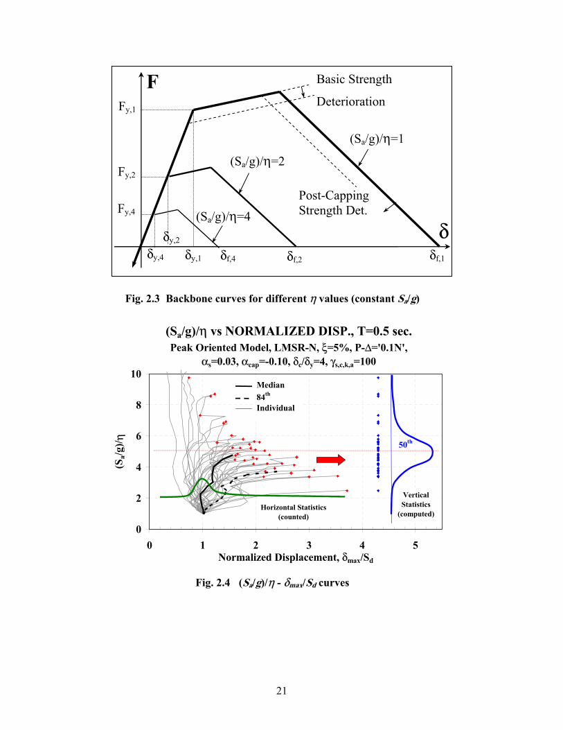
21

Fig. 2.3 Backbone curves for different η values (constant Sa/g)

(Sa/g)/η vs NORMALIZED DISP., T=0.5 sec.Peak Oriented Model, LMSR-N, ξ=5%, P-∆='0.1N',

αs=0.03, αcap=-0.10, δc/δy=4, γs,c,k,a=100

0

2

4

6

8

10

0 1 2 3 4 5Normalized Displacement, δmax/Sd

(Sa/g

)/ η

Median84th

Individual

50th

Horizontal Statistics (counted)

VerticalStatistics

(computed)

Fig. 2.4 (Sa/g)/η - δmax/Sd curves

Basic Strength

Deterioration

δf,2 δf,1 δf,4δy,1 δy,4 δy,2

Post-CappingStrength Det.

(Sa/g)/η=1

Fy,1

δ

(Sa/g)/η=2

(Sa/g)/η=4

Fy,2

Fy,4

F

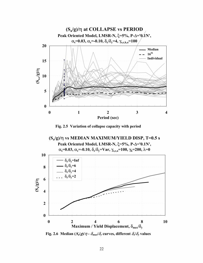
22

(Sa/g)/η at COLLAPSE vs PERIODPeak Oriented Model, LMSR-N, ξ=5%, P-∆='0.1N',

αs=0.03, αc=-0.10, δc/δy=4, γs,c,k,a=100

0

5

10

15

20

0 1 2 3 4Period (sec)

(Sa,

c/g)/ η

Median16th

Individual

Fig. 2.5 Variation of collapse capacity with period

(Sa/g)/η vs MEDIAN MAXIMUM/YIELD DISP, T=0.5 sPeak Oriented Model, LMSR-N, ξ=5%, P-∆='0.1N',αs=0.03, αc=-0.10, δc/δy=Var, γs,c,a=100, γk=200, λ=0

0

2

4

6

8

10

0 2 4 6 8 10Maximum / Yield Displacement, δmax/δy

(Sa/g

)/ η

δc/δy=Infδc/δy=6δc/δy=4δc/δy=2

Fig. 2.6 Median (Sa/g)/η - δmax/δy curves, different δc/δy values

23

Fig. 2.7 Representation of uncertainty in system parameters

CONTRIBUTION TO Var on (Sa,c/g)/η), σlnYi=0.60Peak Oriented Model, LMSR-N, ξ=5%, P-∆=0

0%

20%

40%

60%

80%

100%

0.1 0.2 0.3 0.4 0.5 0.6 0.7 0.8 0.9 1.0 1.2 1.5 1.8 2.1 2.4 2.7 3.0 3.3 3.6 4.0Period, T (sec)

Con

trib

to V

ar[(

S a,c/g

)/ η)]

Record to Record Variability

Post Capping Stiffness

Ductility Capacity

Cyclic Deterioration

Fig. 2.8 Contribution of uncertainty in system parameters to variance of (Sa,c/g)/η

δfδc δy

Fc Fy

F

δ

Symm

Uncertainty in Ductility Capacity, δc/δy

16th 84th50th

Uncertainty in Post-Capping Stiffness, αc

24

(Sa)/η vs PROBABILITY OF COLLAPSE, T=0.5 sPeak Oriented Model, LMSR-N, ξ=5%, P-∆='0.1N'

αs=0.05, αc=Var, δc/δy=Var, γs,c,k,a=Var

0

0.2

0.4

0.6

0.8

1

0 4 8 12 16(Sa/g) / η

Prob

abili

ty o

f Col

laps

e

γs,c,k,a=25, δc/δy=2, αc=-0.50γs,c,k,a=50, δc/δy=4, αc=-0.30 γs,c,k,a=100, δc/δy=4, αc=-0.10 γs,c,k,a=Inf, δc/δy=6, αc=-0.10

Fig. 2.9 Examples of fragility curves for SDOF systems with T = 0.5 s

Fig. 2.10 Assessment of mean annual frequency of collapse

Hazard Curve λSa(x)

Probability of Sa,c/g exceeding “x” given Sa/g ⇒FC,Sa(x)

λSa

Sa/g (Sa/g) PDF for Sa,c/g

x

EDP

CDF for Sa,c/g

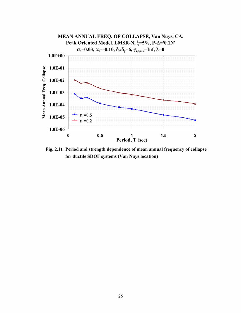
25

MEAN ANNUAL FREQ. OF COLLAPSE, Van Nuys, CA.Peak Oriented Model, LMSR-N, ξ=5%, P-∆='0.1N'

αs=0.03, αc=-0.10, δc/δy=6, γs,c,a,k=Inf, λ=0

1.0E-06

1.0E-05

1.0E-04

1.0E-03

1.0E-02

1.0E-01

1.0E+00

0 0.5 1 1.5 2Period, T (sec)

Mea

n A

nnua

l Fre

q. C

olla

pse

η =0.5η =0.2

Fig. 2.11 Period and strength dependence of mean annual frequency of collapse

for ductile SDOF systems (Van Nuys location)

26

Sa/g vs DISPLACEMENT, η=0.1, T=0.5 sec.Peak Oriented Model, LMSR-N, ξ=5%, P-∆='0.1N',


0

0.2

0.4

0.6

0.8

1

1.2

1.4

1.6

0 2 4 6 8 10Displacement, δmax (in)

S a/g

Median Sa,c/g

Fig. 2.12 IDA curves for an intermediate ductile SDOF system, η = 0.1

1/η vs DISPLACEMENT, Sa/g=0.5, T=0.5 sec.Peak Oriented Model, LMSR-N, ξ=5%, P-∆='0.1N',


0

5

10

15

20

25

30

35

0 5 10 15Displacement, δmax (in)

1/η

Median 1/ηc

Fig. 2.13 Strength variation curves for an intermediate ductile SDOF system, Sa/g = 0.5

27

NEHRP, Response Spectrum, LA 10/50Soil Type D

0

0.2

0.4

0.6

0.8

1

1.2

0 0.5 1 1.5 2 2.5 3 3.5 4

Period, T (sec)

S a/g

Fig. 2.14 NEHRP design spectrum for soil type D, L.A. site

η at COLLAPSE vs PERIODPeak Oriented Model, LMSR-N, ξ=5%, P-∆='0.1N',


0

0.1

0.2

0.3

0.4

0.5

0.6


η

Computed Median η

Fig. 2.15 Median strength associated with collapse for an intermediate ductile system,

Sa(T)/g according to NEHRP design spectrum

3 Hysteretic Models

3.1 INTRODUCTION

Collapse assessment requires hysteretic models capable of representing all the important modes

of deterioration that are observed in experimental studies. Figure 3.1 illustrates a monotonic

load-displacement response and a superimposed quasi-static cyclic response of “identical”

plywood shear wall panels (Gatto and Uang, 2002). The monotonic test result shows that

strength is “capped” and is followed by a negative tangent stiffness. The cyclic hysteretic

response indicates that the strength in large cycles deteriorates with the number and amplitude of

cycles, even if the displacement associated with the strength cap has not been reached (1). It also

indicates that strength deterioration occurs in the post-capping range (2), and that the unloading

stiffness may also deteriorate (3). Furthermore, it is observed that the reloading stiffness may

deteriorate at an accelerated rate (4).

Several hysteretic models have been developed to represent the behavior of components

that exhibit characteristics of the type illustrated in Figure 3.1 (Kunnath et al., 1991, Sivaselvan

and Reinhorn, 2000; Song and Pincheira, 2000). However, few models integrate all the important

deterioration sources such as strength deterioration in the backbone curve (post-capping stiffness

branch) and cyclic deterioration of strength and stiffness. For this reason, deteriorating models

were developed in this study for bilinear, peak-oriented, and pinched hysteretic systems. The

models are implemented in an in-house computer program called SNAP that carries out dynamic

and quasi-static inelastic analysis for SDOF systems6. The component deterioration models are

also implemented in a computer program for MDOF systems that carries out dynamic nonlinear

analyses, DRAIN-2DX (1993). The models incorporate a backbone curve that represents the

monotonic response. Under cyclic behavior, several system parameters may deteriorate after

6 SNAP is based on the program NLDYNA developed by Rahnama (Rahnama and Krawinkler, 1993).

30

each excursion. The sources of cyclic deterioration are basic strength, post-capping strength,

unloading stiffness, and accelerated reloading stiffness deterioration.

1.1 3.2 BASIC HYSTERETIC MODELS

The following is a description of the three hysteretic models used in this study and the

modifications introduced when post-capping strength deterioration is included in the backbone

curve.

3.2.1 Description of Backbone Curve

The backbone curve defines the monotonic response and is the same for all hysteretic models

(Fig. 3.2). This also defines the boundaries for the load-displacement relationship. The backbone

curve is defined by the following parameters:

Initial Stiffness (Ke). It defines the elastic branch of the curve and is located between the

origin (0, 0) and the yielding point (δy, Fy).

Hardening Stiffness (Ks). This stiffness is defined by connecting the yield point to the

peak point (δc, Fc). The hardening stiffness is defined as a fraction of the initial stiffness:

ess KK α= (3.1)

The cap displacement (δc) is the point where the post-capping branch begins. If δc is

normalized by the yielding displacement, the ratio is called ductility capacity, δc/δy. The peak

strength (Fc) is attained at the end of the hardening branch:

)( ycsyc KFF δδ −+= (3.2)

Post-Capping Stiffness (Kc). This stiffness is defined by connecting the peak point to the

beginning of the residual strength branch (δr, Fr). The post-capping stiffness is also defined as a

fraction of the initial stiffness:

ecc KK α= (3.3)

Residual Strength Branch. The residual strength is a fraction of the initial yield

strength:

yr FF λ= (3.4)

31

Residual strength is not modified when cyclic deterioration shrinks the backbone curve.

The displacement at which the residual strength branch starts, δr, is calculated as:

crccr KFF /)( −+= δδ (3.5)

The parameters sα , yc δδ / , cα and λ are obtained from calibration of the hysteretic

models with load-deformation data obtained from experiments (see Section 3.5).

3.2.2 Bilinear Model

This model is based on the standard bilinear hysteretic rules with kinematic strain hardening.

These basic rules are preserved once post-capping and residual strength branches are included.

However, it is necessary to introduce the “strength limit” shown in Figure 3.3 when the

backbone curve includes a branch with negative slope. The limit for strength corresponds to the

smallest strength reported on the post-capping branch in previous excursions. In Figure 3.3, the

loading curve starting at 5 should continue up to intersect 6′, according to kinematic rules.

However, this loading segment ends when it intersects the “strength limit” at point 6. The limit

corresponds to the strength of point 3, which is the smallest strength in the nonlinear range of the

backbone curve in earlier cycles. If this condition were not established, the strength in the

loading path could increase in later stages of deterioration.

3.2.3 Peak-Oriented Model

This model keeps the basic hysteretic rules proposed by Clough and Johnston in 1965, but the

backbone curve is modified to include strength capping and residual strength. The presence of a

negative post-capping stiffness does not modify any basic rules of the model. Figure 3.4a shows

the deterioration of the reloading stiffness for a peak-oriented model once the horizontal axis is

reached (points 3 and 7). The reloading path targets the previous maximum displacement.

Mahin and Bertero (1975) proposed that the reloading path be directed to the maximum

displacement of the last cycle instead of the maximum displacement of all former cycles if the

former path results in a larger reloading stiffness. This is exemplified in Figure 3.4b, where the

reloading from point 10 is directed to point 7 (maximum displacement of last cycle) instead of

point 2 (maximum displacement of all earlier cycles), as in the original peak-oriented model.

Once point 7 is reached, the path is redirected to point 2.

32

3.2.4 Pinching Model

The pinching model is similar to the peak-oriented one, except that reloading consists of two

parts. Initially the reloading path is directed toward a point denoted as “break point,” which is a

function of the maximum permanent deformation and the maximum load experienced in the

direction of loading. The break point is defined by the parameter κf, which modifies the

maximum “pinched” strength (points 4 and 8 of Fig. 3.5a), and κd, which defines the

displacement of the break point (points 4′ and 8′). The first part of the reloading branch is

defined by Krel,a and once the break point is reached (points 4′ and 8′), the reloading path is

directed toward the maximum deformation of earlier cycles in the direction of loading (Krel,b)

Reloading without Krel,a. If the absolute deformation at reloading (point 13, Fig. 3.5b) is

larger than the absolute value of perd δκ )1( − , the reloading path consists of a single branch that

is directed toward the previous maximum deformation in the direction of loading.

1.2 3.3 CYCLIC DETERIORATION

3.3.1 Deterioration Based on Hysteretic Energy Dissipation

Four cyclic deterioration modes may be activated once the yielding point is surpassed in at least

one direction: basic strength, post-capping strength, unloading stiffness, and reloading stiffness

deterioration. The basic cyclic deterioration rules are the same for all the hysteretic models with

the exception of the accelerated stiffness deterioration, which does not exist in the bilinear

model. The peak-oriented model will be used to illustrate the effect of cyclic deterioration.

The cyclic deterioration rates are controlled by the rule developed by Rahnama and

Krawinkler (1993), which is based on the hysteretic energy dissipated when the component is

subjected to cyclic loading. It is assumed that the hysteretic energy-dissipation capacity is a

known quantity that is independent of the loading history.

The cyclic deterioration in excursion i is defined by the parameter βi, which is given by

the following expression: C

i

jjt

ii

EE

E

⎟⎟⎟⎟⎟

⎠

⎞

⎜⎜⎜⎜⎜

⎝

⎛

−=

∑=1

β (3.6)

33

where

iE = hysteretic energy dissipated in excursion i

Σ jE = hysteretic energy dissipated in all previous excursions (both positive and

negative)

tE = hysteretic energy-dissipation capacity, yyt FE δγ=

γ expresses the hysteretic energy-dissipation capacity as a function of twice the

elastic strain energy at yielding (Fyδy). It is calibrated from experimental

results and can be different for each deterioration parameter.

c = exponent defining the rate of deterioration of the evaluated hysteretic

parameter (strength or stiffness). Rahnama and Krawinkler (1983) suggested

that a reasonable range for c is between 1.0 and 2.0. If the displacement history

consists of constant amplitude cycles, a unit value for c implies an almost

constant rate of deterioration of the hysteretic parameter. For the same

displacement history, a value c = 2 slows down the rate of deterioration in

early cycles and accelerates the rate of deterioration in later cycles.

Throughout the time history analysis, βi must be within the limits 10 ≤< iβ . If this

inequality does not hold ( 0≤iβ or 1>iβ ), the hysteretic energy capacity is exhausted and

collapse takes place. Mathematically:

i

i

jjyy EEF <−∑

=1δγ (3.7)

3.3.2 Basic Strength Deterioration

It is defined by translating the strain-hardening branch toward the origin by an amount equivalent

to reducing the yield strength to: +−

+ −= 1, )1( iisi FF β and −−

− −= 1, )1( iisi FF β (3.8)

in which −+ /

iF = deteriorated yield strength after excursion i.

−+−

/1i

F = deteriorated yield strength before excursion i.

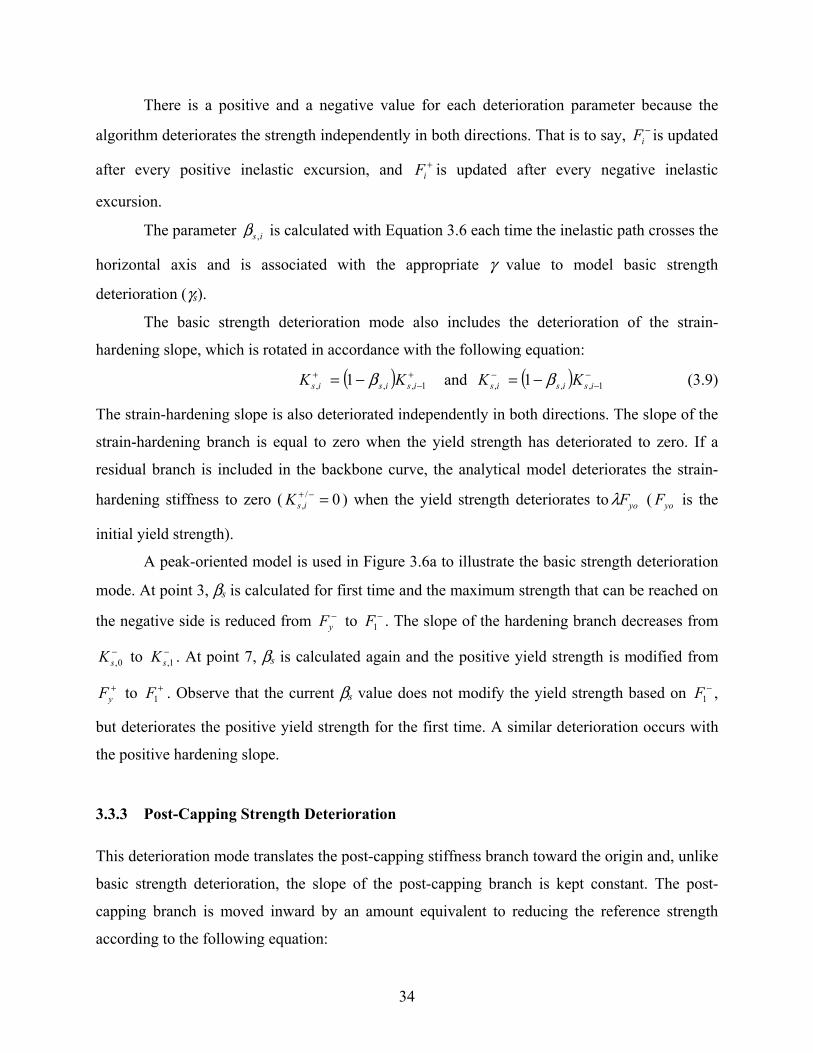
34

There is a positive and a negative value for each deterioration parameter because the

algorithm deteriorates the strength independently in both directions. That is to say, −iF is updated

after every positive inelastic excursion, and +iF is updated after every negative inelastic

excursion.

The parameter is ,β is calculated with Equation 3.6 each time the inelastic path crosses the

horizontal axis and is associated with the appropriate γ value to model basic strength

deterioration (γs).

The basic strength deterioration mode also includes the deterioration of the strain-

hardening slope, which is rotated in accordance with the following equation:

( ) +−

+ −= 1,,, 1 isisis KK β and ( ) −−

− −= 1,,, 1 isisis KK β (3.9)

The strain-hardening slope is also deteriorated independently in both directions. The slope of the

strain-hardening branch is equal to zero when the yield strength has deteriorated to zero. If a

residual branch is included in the backbone curve, the analytical model deteriorates the strain-

hardening stiffness to zero ( 0/, =−+isK ) when the yield strength deteriorates to yoFλ ( yoF is the

initial yield strength).

A peak-oriented model is used in Figure 3.6a to illustrate the basic strength deterioration

mode. At point 3, βs is calculated for first time and the maximum strength that can be reached on

the negative side is reduced from −yF to −

1F . The slope of the hardening branch decreases from

−0,sK to −

1,sK . At point 7, βs is calculated again and the positive yield strength is modified from

+yF to +

1F . Observe that the current βs value does not modify the yield strength based on −1F ,

but deteriorates the positive yield strength for the first time. A similar deterioration occurs with

the positive hardening slope.

3.3.3 Post-Capping Strength Deterioration

This deterioration mode translates the post-capping stiffness branch toward the origin and, unlike

basic strength deterioration, the slope of the post-capping branch is kept constant. The post-

capping branch is moved inward by an amount equivalent to reducing the reference strength

according to the following equation:

35

( ) −+−+−

−= /,

/1,,

1irefiref

FF icβ (3.10)

−+ /refF is the intersection of the vertical axis with the projection of the post-capping branch

(Fig. 3.6b). There is a positive and negative reference strength parameter for independently

deteriorating the positive and negative post-capping strength. βc is associated with an appropriate

γ value to model post-capping strength deterioration (γc).

The deterioration of post-capping strength is computed each time the horizontal axis is

crossed, but the deterioration parameter may not affect the loading path in the early stages of

nonlinearity. In Figure 3.6b, the first post-capping deterioration is calculated at point 3 and the

negative reference point moves to −1,refF . This backbone modification does not affect the loading

path due to the small magnitude of the negative displacement. At point 6, the deterioration of the

post-cap strength is computed again and this time the loading path is modified because the

updated cap displacement ( +1cδ ) is exceeded in this excursion.

3.3.4 Unloading Stiffness Deterioration

The unloading stiffness (Ku) is deteriorated in accordance with the following equation:

1,,, )1( −−= iuikiu KK β (3.11)

where

iuK , = deteriorated unloading stiffness after excursion i

1, −iuK = deteriorated unloading stiffness before excursion i

ik ,β is associated with an appropriated cyclic deterioration parameter γk.

The parameter kβ is the only one that is calculated when a load reversal takes place in

the inelastic range. Furthermore, this is the only deterioration mode in which the deterioration

parameter in one direction is also used to update the deterioration parameter in the other

direction. Consequently, the unloading stiffness is updated up to twice as much as the other

deterioration parameters. Thus, if the same energy-dissipation capacity is expected for the four

deterioration modes, it is recommended to assign a larger value to γk than to γs, γc and γa. If the

same energy is dissipated in the positive and negative directions, then γk should be about twice as

large as the other γ values, i.e., acsk ,,2γγ = .

36

Figure 3.6c shows a peak-oriented model that includes unloading stiffness deterioration.

At point 2 the first reversal in the inelastic range occurs and the unloading stiffness deteriorates

from Ke to a deteriorated value Ku,1. At point 5 the first reversal on the negative side takes place

and Ku,2 is calculated based on the updated βu and Ku,1. Unlike other deterioration modes, Ku,2 is

updated based on the value of the unloading stiffness on the other side of the loop.

The deterioration of unloading stiffness takes place each time that a reversal occurs and the

updated unloading stiffness is used for subsequent updates of this parameter. However, the

unloading stiffness update is disregarded if the reversal is considered an interruption in the

direction of loading. In peak-oriented and pinching models, an interruption occurs when the path

is on the unloading stiffness and a reversal takes place before the path targets the maximum

displacement on the opposite side (Fig. 3.6c). In bilinear models, an interruption occurs when the

path is on the unloading stiffness and has a reversal before reaching the backbone curve on the

opposite side.

3.3.5 Accelerated Reloading Stiffness Deterioration

This deterioration mode increases the absolute value of the target displacement, defined as the

maximum positive or negative displacement of past cycles, according to the direction of loading.

Accelerated reloading stiffness deterioration is defined only for peak-oriented and pinching

models and is governed by the following equation: −+−+

−+= /

,/

1,,)1(

itit ia δβδ (3.12)

There is a target displacement (δt) for each loading direction, and the reloading stiffness

deterioration is calculated each time the horizontal axis is crossed (Fig. 3.6d). Equation 3.6 is

employed to compute βa based on the corresponding parameter γa.

1.3 3.4 CALIBRATION OF HYSTERETIC MODELS WITH COMPONENT TESTS

The proposed hysteretic models have been calibrated with load-deformation data obtained from

experiments on steel, reinforced concrete, and wood components. The best way of defining the

backbone curve parameters (ductility capacity and post-capping stiffness) is with a monotonic

test because cyclic deterioration effects are not present. The parameter γ is estimated from

37

experiments in which the specimen is subjected to cyclic loading. The following are examples of

some calibrations for different materials.

3.4.1 Steel Specimens

Figures 3.7–3.8 illustrate the calibration of the bilinear model on beam load-displacement

relationships for steel beam-column subassemblies (Uang et al., 2000). Because monotonic tests

were not available to obtain the backbone curve for the simulations, the parameters of the

backbone curve (Fy, δy, δc, αs, and αc) were estimated from the load-displacement relationship of

the second excursion of the near-fault tests. This second excursion is considered to be equivalent

to a monotonic load-displacement relationship because only small structural damage occurred

during the first excursion in the opposite direction. Based on this approach, the following

properties are utilized for all four simulations: Fy = 103 kips, δy = 1.03 in., αs = 0.03, αc = -0.03,

δc /δy = 2.75, and no residual strength (λ = 0). The cyclic deterioration parameters are: c = 1.0

and γs = γc = γk = γa = 130. The use of different γ values for each deterioration mode could have

resulted in a better calibration. However, γ’s are set at the same value because the objective is to

find representative parameters that can be used when no experimental results are available.

Specimens LS1 and LS4 were tested using the standard SAC loading protocol (Fig. 3.7).

The main difference between them is that the beam in specimen LS4 is braced to help it achieve

its full plastic moment capacity. The analytical model provides a good correlation with the

experimental loops. However, the response at early cycles cannot be fully reproduced because

steel components develop cyclic strain hardening, a feature that is not included in the analytical

model.

Specimens LS2 and LS3 were tested using the SAC near-fault loading protocol. The

specimens were loaded in opposite directions. As in the former case, the absence of cyclic strain

hardening in the analytical model can be observed in the early cycles of the history where the

load-deformation response of the model underestimates that of the experiment. In general, good

correlation is observed between experimental and analytical loops for the four tests, although the

same hysteretic properties are utilized for different loading protocols.

Figures 3.9–3.10 show plots of negative and positive normalized hysteretic energy (NHE

= total hysteretic energy dissipated / Fyδy) as a function of the number of cycles for all four

specimens. In all cases the history of NHE is similar for both the analytical model and the

38

experimental results. Thus, the bilinear hysteretic model is able to replicate the cumulative

energy dissipated under the action of various loading protocols. Note that the sum of positive and

negative NHE is smaller than the analytical input parameter γs,c,k = 130. The reason is that

although γ ’s were directly calibrated from experimental results, complete loss of restoring force

is not reached in any case. According to the hysteretic loops, specimen LS-2 is the closest to lose

all its restoring force. Consequently, this is the case where the sum of positive and negative NHE

is closest to the input parameter γs,c,k = 130 because the hysteretic energy capacity is almost

exhausted.

3.4.2 Wood Specimens

Figure 3.11 illustrates the calibration of the pinching model on plywood shear wall load-

displacement relationships (Gatto and Uang, 2002). Four different loading protocols are used in

the calibrations: ISO, SPD, CUREE standard, and CUREE-near-fault. The CUREE loading

protocols were developed by Krawinkler et al. (2001) for wood-frame testing. The following

properties for the backbone curve were obtained from a monotonic test and were utilized in the

simulations: Fy = 7 kips, δy = 1.0 in., αs = 0.10, αc = -0.13, δc /δy = 4, λ = 0, and κf = κd = 0.25.

The cyclic deterioration parameters used were: c = 1.0, γs = γc = γa = 50, and γk = ∞ (no

unloading stiffness deterioration). The graphs show that the pinching hysteretic model is able to

simulate cyclic deterioration observed in the plywood shear wall panel tests for the four loading

protocols.

Figure 3.12 shows plots of positive and negative NHE as a function of the number of

cycles. In all cases, the history of the NHE of the analytical model is below the one

corresponding to the experimental results because the model remains elastic until δy is achieved.

That is to say, the models do not dissipate energy below this threshold, whereas the experimental

results exhibit energy dissipation at displacement levels well below the estimated value of δy.

Although the trends in the history of NHE between the model and test results are slightly offset

by this difference, the pinching model is able to replicate the cumulative energy dissipated,

especially at relatively large deformation levels.

39

3.4.3 Reinforced Concrete Specimens

The calibration of reinforced concrete (RC) specimens utilizes the experiments carried out by

Moehle and Sezen (Sezen, 2000). They tested four columns with deficient transverse

reinforcement, which were connected to very rigid top and base beams to produce double

curvature. The two columns (“1” and “4”) with small constant axial load P = 0.15f′cAg are

calibrated in this study. Column “1” was subjected to a stepwise increasing cyclic loading

protocol and column “4” to a mostly monotonic history, consisting of several small cycles

followed by a big final excursion. For calibration purposes, the backbone parameters were based

on the results of column 4 and the cyclic deterioration parameters on the results of column 1.

Figure 3.13 presents the experimental and analytical hysteretic loops of columns 1 and 4 along

with the input parameters. Both cases exemplify the difficulties in reproducing early inelastic

cycles in reinforced concrete components when the analytical models do not include the cracking

point. However, the pinching model simulates well the highly inelastic behavior.

Figure 3.14 depicts the NHE dissipation histories for the aforementioned cases. For

column 4, the NHE is negligible up to the last cycle, in which most of the energy is dissipated.

For column 1, the sum of positive and negative NHE is also very small compared to γ = 50. The

reason is that the large slope of the post-capping branch is preventing the total NHE from

reaching a value close to γ, even for systems that are very close to complete failure.

1.4 3.5 ILLUSTRATIONS OF CYCLIC DETERIORATION EFFECTS

As shown in previous sections, the deteriorating model is capable of reproducing the response of

tests of components made of steel, reinforced concrete, and wood. Calibrations with component

tests have provided typical values for the deteriorating system parameters. This section illustrates

the effects various deterioration parameters have on the hysteretic response when a component is

subjected to the CUREE loading protocol (Krawinkler et al., 2000) (Fig. 3.15). Three parameters

are of primary interest: the ductility capacity δc /δy, the post-capping stiffness αc, and the series

of cyclic deterioration parameters γs, γc, γk, and γa. In these illustrations it is assumed that all four

cyclic deterioration parameters are equal.

Figure 3.16 shows nine hysteretic responses that have the same post-capping stiffness,

αc = -0.10, in common. From left to right in the figure the ductility capacity decreases from δc /δy

40

= 6 to δc /δy = 4 and 2, whereas from top to bottom in the figure the cyclic deterioration

parameter decreases from γs,c,k,a = infinite to γs,c,k,a = 100 and 25. Thus, the effect of a decrease in

the ductility capacity can be studied by viewing the figure from left to right and the effect of a

decrease in the cyclic deterioration parameter can be studied by viewing the figure from top to

bottom. There are clear patterns both in the horizontal and vertical directions. It is noted, for

instance, that for this specific loading history the ductility capacity becomes rather irrelevant if

the cyclic deterioration parameter is small (γs,c,k,a = 25), i.e., cyclic deterioration effects

overpower the effect of monotonic ductility (see bottom row of the figure). This observation is

consistent but not very relevant because the combination of a monotonically ductile component

that experiences rapid cyclic deterioration is rather unlikely. For all other cases illustrated, the

combination of ductility capacity and cyclic deterioration parameters control the response.

Figure 3.17 presents the same arrangement of systems, but using a steep post-capping

slope corresponding to αc = -0.50. There are clear differences between each graph of Figures

3.16–3.17, demonstrating the importance of the post-capping stiffness. For the steep post-

capping slope corresponding to αc = -0.50, the monotonic ductility capacity becomes much

important because little “life” is left at deformations exceeding the monotonic ductility capacity.

The important observation to be made is that the effects of none of the deterioration

parameters can be evaluated in isolation. It is the combination of all three deterioration

parameters (δc /δy, αc, γs,c,k,a) that governs the cyclic behavior.

1.5 3.6 ADDITIONAL OBSERVATIONS ON DETERIORATION MODEL

The power of the proposed deterioration model is in its versatility that makes it feasible to

represent many deterioration modes in a transparent and physically justifiable manner. If the

simplifications are acceptable that all cyclic deterioration modes can be represented by the same

γ value, and that the exponent in Equation 3.6 can be taken as 1.0, then all cyclic deterioration

modes are controlled by a single parameter, γs,c,k,a. There is no simpler way possible to describe

cyclic deterioration. It is the combination of this single cyclic deterioration parameter with a

backbone curve incorporating monotonic strength capping and a post-capping stiffness that

makes this deterioration model simple but versatile. The following observations are believed to

be of importance in the context of damage and deterioration modeling.

41

There are fundamental differences between this deterioration model and cumulative

damage models. The latter merely count cumulative damage and use a counter to indicate degree

of damage and complete “failure” (usually identified by the counter taking on a value of 1.0).

They do not consider that cumulative damage causes a decrease in strength and stiffness and

therefore leads to an increase in deformations. It is the loss of strength and the increase in

deformation that ultimately will cause collapse of a structure. Moreover, cumulative damage

models apply to components and not to structures. Many attempts are reported in the literature to

extrapolate from component cumulative damage models to structural damage models, but none

of these attempts are believed to have been successful in tracing damage close to collapse.

Collapse is caused by deterioration in complex assemblies of components, and such deterioration

must be modeled explicitly.

• The proposed deterioration model incorporates cyclic deterioration controlled by

hysteretic energy dissipation as well as deterioration of the backbone curve (strength

capping at δc/δy and a post-capping decrease in strength defined by αc). This dual

deterioration behavior is equivalent to the two-part damage concept contained in some

cumulative damage models such as the Park-Ang model (Park and Ang, 1985). This

model, which was developed specifically for reinforced concrete components, consists of

a linear combination of displacement and energy demands, expressed as follows:

HEdF

+ = DMultyult

max ∫δβ

δδ

(3.13)

where, DM = damage measure

δmax = the maximum displacement of the system

δult = the monotonic displacement capacity of the system

β = structural performance parameter

In concept, the parameters δult and β of this cumulative damage model are equivalent to

δc and γ of the proposed deterioration model.

• Inspection of Figures 3.9–3.10, 3.12, and 3.14 shows that the hysteretic energy-

dissipation capacity γFyδy is rarely achieved in component tests. Components usually

reach zero resistance long before this capacity is utilized. This happens because of

42

strength capping and post-capping strength decrease and is equivalent to the importance

of the first term of the Park-Ang model given by Equation 3.13.

• In all studies reported in this report it is assumed that the exponent c in Equation 3.6 is

1.0. Based on cumulative damage concepts it can be argued that c should be greater than

1.0 (likely on the order of 1.5–2.0). This “simplification” is not believed to have a large

effect on the response of deteriorating systems. An exponent greater than 1.0 will

accelerate deterioration, but primarily for very large excursions. For such excursions,

strength capping and post-capping strength decrease dominate over cyclic deterioration.

1.6 3.7 SUMMARY

This chapter describes the model developed for deteriorating structural components. The sources

of deterioration considered are strength deterioration in the backbone curve and cyclic strength

and stiffness deterioration. The models have been codified in an in-house SDOF program called

SNAP and implemented in nonlinear analysis programs for MDOF structures that consider

nonlinearities by means of concentrated plasticity (DRAIN-2DX and OpenSees).

The hysteretic models have been calibrated with experiments of components made of

steel, wood, and reinforced concrete. Some of the experimental programs consist of several

identical specimens subjected to different loading protocols. In the calibration process, the same

system and deterioration parameters are used for all the loading protocols. The correlation for

most of the cases is good, suggesting that the backbone characteristics and the parameter γ for

cyclic deterioration are adequate to represent component behavior regardless of the loading

protocol.

The effect of individual deterioration parameters on the hysteretic response depends

largely on the relative values of all the other parameters. This can be observed from Figures

3.16–3.17, in which hysteretic responses for systems with variations of a particular parameter are

compared.

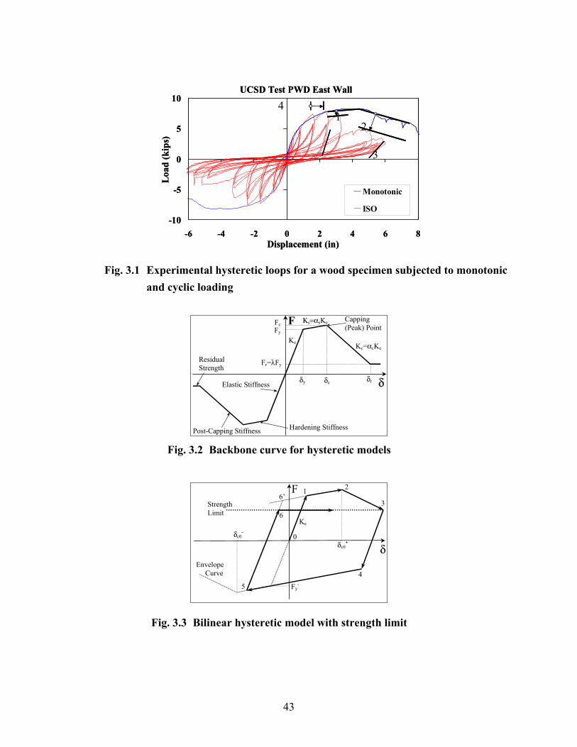
43

UCSD Test PWD East Wall

-10

-5

0

5

10

-6 -4 -2 0 2 4 6 8Displacement (in)

Loa

d (k

ips)

Monotonic

ISO

UCSD Test PWD East Wall

-10

-5

0

5

10

-6 -4 -2 0 2 4 6 8Displacement (in)

Loa

d (k

ips)

Monotonic

ISO

Fig. 3.1 Experimental hysteretic loops for a wood specimen subjected to monotonic and cyclic loading

Kc=αcKe

δcδy δr

Residual Strength

Capping (Peak) Point

Ke

Hardening Stiffness Post-Capping Stiffness

Elastic Stiffness

Fy

Fc

δ

F Κs=αsKe

Fr=λFy

Fig. 3.2 Backbone curve for hysteretic models

2

5

Ke

3

δ

Fy-

6

0

1

δc0+

δc0-

Envelope Curve 4

Strength Limit

6’F

Fig. 3.3 Bilinear hysteretic model with strength limit

3

12

4

44

(a) (b)

Fig. 3.4 Peak-Oriented hysteretic model; (a) basic model rules, (b) Mahin and Bertero’s modification (Mahin and Bertero, 1975)

(a) (b)

Fig. 3.5 Pinching hysteretic model; (a) basic model rules, (b) reloading deformation at the right of break point

Fp2=κf.Fmax

Krel,a

Ke

Fy+

3

δ

F

κd.δper1

0

12

6 5

7 4’

8’

Fy-

Fmax

δper1 4

8

Fp1=κf.Fy-

Fmin

Krel,a

Krel,b

Krel,b

“break point”

Krel,b

Fy+

3 0

1

6 5

7Krel,a

4’

8’

δper2+

11

10

12

13

Fy-

Krel,a

Krel,b

δ

κd.δper2+

2,914

F

“break point”

6

2,8

δc0-

Ke

Fy+

3

δ

F

Krel

0

1

5

δc0+

4

Krel

Fy-

7

9 10

11

Fy+

Krel Krel

3

δ6 0

1 2

54

7,11

8

9

10

12F

Klast

Fy-

45

(a) Basic Strength Deterioration (b) Post-capping Strength Deterioration

(c) Unloading Stiffness Deterioration (d) Accelerated Reloading Stiffness Det.

Fig. 3.6 Peak-oriented model with individual deterioration modes

F

δ

Ku,1

0

Ke Fy

+

Ku,2

Fy-

1 2

3

4 5

6

7 Interruption (disregard stiffness det)

Ke

δ6

∆δt1-

Krel

Fy+

3

Fy-

Ke

0

1 2

4 5

7

δc0+

Original Envelope

δc0-

8 9 F ∆δt1

+

2

4

7

6

Fy+

3

Krel

0

1

δc0+δc1

+

Original Envelope

δc1-

Fref,0+

δc0-

Fref,1+

Fref,1-

Fy-

Ke

Fref,0-

δ

F

8

1

Ke

3

F1+

6

0

2

4 5

8

δco+

δc0- δc1

-

Ks,0

Ks,1+

Ks,1-

Fy+

Fy-

F1-

δc1+ 7

δ

F

Ks,0

46

UCSD STEEL TEST-LS1 (SYMMETRIC LOADING)Bilinear Model, Fy=103 kips, δy=1.03 in

αs=0.03, αc=-0.03, δc/δy=2.75, γs,c,k=130, γa=N.A., λ=0

-1.2

-0.8

-0.4

0

0.4

0.8

1.2

-12 -10 -8 -6 -4 -2 0 2 4 6 8 10 12Normalized beam displacement, δ/δy

Nor

mal

ized

Loa

d, F

/Fy

ExperimentModel

Backbone

UCSD STEEL TEST-LS4 (SYMMETRIC LOADING)Bilinear Model, Fy=103 kips, δy=1.03 in


-1.2

-0.8

-0.4

0

0.4

0.8

1.2


Nor

mal

ized

Loa

d, F

/Fy

ExperimentModel

Backbone

(a) Test LS-1 (b) Test LS-4

Fig. 3.7 Calibration of bilinear model on steel component tests using the SAC standard loading protocol (Uang et al., 2000)

UCSD STEEL TEST-LS2 (NEAR FAULT LOADING)

Bilinear Model, Fy=103 kips, δy=1.03 inαs=0.03, αc=-0.03, δc/δy=2.75, γs,c,k=130, γa=N.A., λ=0

-1.2

-0.8

-0.4

0

0.4

0.8

1.2


Nor

mal

ized

Loa

d, F

/Fy

ExperimentModel

Backbone

UCSD STEEL TEST-LS3 (NEAR FAULT LOADING)Bilinear Model, Fy=103 kips, δy=1.03 in


-1.2

-0.8

-0.4

0

0.4

0.8

1.2


Nor

mal

ized

Loa

d, F

/Fy

ExperimentModel

Backbone

(a) Test LS-2 (b) Test LS-3 Fig. 3.8 Calibration of bilinear model on steel component tests using the SAC near-fault

protocol (Uang et al., 2000)

NHE-UCSD STEEL TEST-LS1 (SYMMETRIC LOADING)

0

20

40

60

0 10 20 30 40Number of Excursions

NH

E =

HE

/ (F

yδy)

Experimental, Pos NHEExperimental, Neg NHEModel, Positive NHEModel, Negative NHE

NHE-UCSD STEEL TEST-LS4 (SYMMETRIC LOADING)

0

20

40

60


NH

E =

HE

/ (F

yδy)

Experimental, Positive NHEExperimental, Negative NHEModel, Positive NHEModel, Negative NHE


Fig. 3.9 History of NHE dissipation, SAC standard loading protocol test of Fig. 3.7, bilinear model

47

NHE-UCSD STEEL TEST-LS2 (NEAR FAULT LOADING)

0

20

40

60


NH

E =

HE

/ (F

yδy)


NHE-UCSD STEEL TEST-LS3 (NEAR FAULT LOADING)

0

20

40

60


NH

E =

HE

/ (F

yδy)



Fig. 3.10 History of NHE dissipation, SAC near-fault loading protocol tests of Fig. 3.8, bilinear model

UCSD TEST PWD EAST WALL (ISO LOADING)

Pinching Model, Fy=7 kips, δy=1.0 in, κs=0.25, κd=0.25,αs=0.10, αc=-0.13, δc/δy=4, γs=50, γc=50, γk=∞, γa=50, λ=0

-1.5

-1

-0.5

0

0.5

1

1.5

-8 -6 -4 -2 0 2 4 6 8Normalized wall displacement, δ/δy

Nor

mal

ized

load

, F/F

y

ModelExperiment

UCSD TEST PWD EAST WALL (CUREE LOADING)Pinching Model, Fy=7 kips, δy=1.0 in, κs=0.25, κd=0.25,

αs=0.10, αc=-0.13, δc/δy=4, γs=50, γc=50, γk=∞, γa=50, λ=0

-1.5

-1

-0.5

0

0.5

1

1.5


Nor

mal

ized

load

, F/F

y

ModelExperiment

(a) ISO Loading Protocol (b) CUREE Standard Loading Protocol

UCSD TEST PWD EAST WALL (SPD LOADING)Pinching Model, Fy=7 kips, δy=1.0 in, κs=0.25, κd=0.25,


-1.5

-1

-0.5

0

0.5

1

1.5


Nor

mal

ized

load

, F/F

y

ModelExperiment

UCSD TEST PWD EAST WALL (NF LOADING)Pinching Model, Fy=7 kips, δy=1.0 in, κs=0.25, κd=0.25,


-1.5

-1

-0.5

0

0.5

1

1.5


Nor

mal

ized

load

, F/F

y

ModelExperiment

(c) SPD Loading Protocol (d) CUREE Near-Fault Loading Protocol

Fig. 3.11 Calibration of pinching model on plywood shear-wall component tests (Gatto and Uang, 2002)

48

NHE-UCSD PWD EAST WALL TEST (ISO LOADING)

0

10

20

30

0 10 20 30 40 50Number of cycles

NH

E =

HE

/(Fy*

δ y)

NHE + ExperimentNHE - ExperimentNHE + ModelNHE - Model

NHE-UCSD PWD EAST WALL TEST (CUREE LOADING)

0

10

20

30


NH

E =

HE

/(Fy*

δ y)


(a) ISO Loading Protocol (b) CUREE Standard Loading Protocol

NHE-UCSD PWD EAST WALL TEST (SPD LOADING)

0

10

20

30


NH

E =

HE

/(Fy*

δ y)


NHE-UCSD PWD EAST WALL TEST (NF LOADING)

0

10

20

30


NH

E =

HE

/(Fy*

δ y)


(c) SPD Loading Protocol (d) CUREE Near-Fault Loading Protocol

Fig. 3.12 History of NHE dissipation, pinching model and loading protocols for tests

of Fig. 3.11

R/C CALIBRATION (MOEHLE & SEZEN, Column 1)Pinching Model, Fy = 12900 kips, δy = 1.03 inαs=0.10, αc=-024, δc/δy=2.3, γs,c,k,a=50, κf,d=0.5, λ=0

-1.2

-0.8

-0.4

0

0.4

0.8

1.2

-6 -4 -2 0 2 4 6Normalized Displacement, δ/δy

Nor

mal

ized

Loa

d, F

/Fy

ModelExperimental

R/C CALIBRATION (MOEHLE & SEZEN, Column 4)Pinching Model, Fy = 12900 kips, δy = 1.03 inαs=0.10, αc=-0.24, δc/δy=2.3, γs,c,k,a=50, κf,d=0.5, λ=0

-1.2

-0.8

-0.4

0

0.4

0.8

1.2


Nor

mal

ized

Loa

d, F

/Fy

ModelExperimental

(a) Cyclic Loading Protocol (b) Mostly Monotonic Loading Protocol

Fig. 3.13 Calibration of pinching model on reinforced concrete columns of Moehle and Sezen experiments (Sezen, 2000)

49

NHE-RC (MOEHLE & SEZEN, Column 1)

0

2

4

6

8

10

0 5 10 15 20 25Number of Excursions

NH

E =

HE

/ (F

yδy)


NHE-RC (MOEHLE & SEZEN, Column 4)

0

2

4

6

8

10

0 5 10 15 20 25Number of Excursions

NH

E =

HE

/ (F

yδy)


(a) Cyclic Loading Protocol (b) Mostly Monotonic Loading Protocol

Fig. 3.14 History of NHE dissipation, pinching model and tests of Fig. 3.13

CUREE STANDARD LOADING PROTOCOL

-1.2-1.0-0.8-0.6-0.4-0.20.00.20.40.60.81.01.2

0 2000 4000 6000 8000Number of Cycles

Nor

mal

ized

∆

0 10 20 30 40

Fig. 3.15 CUREE standard loading protocol

50

-1.2

-0.8

-0.4

0

0.4

0.8

1.2


Nor

mal

ized

For

ce, F

/Fy

αc = -0.10 δc/δy = 6 γs,c,k,a = Inf

-1.2

-0.8

-0.4

0

0.4

0.8

1.2


Nor

mal

ized

For

ce, F

/Fy


-1.2

-0.8

-0.4

0

0.4

0.8

1.2


Nor

mal

ized

For

ce, F

/Fy


-1.2

-0.8

-0.4

0

0.4

0.8

1.2


Nor

mal

ized

For

ce, F

/Fy

αc = -0.10 δc/δy = 6 γs,c,k,a = 100

-1.2

-0.8

-0.4

0

0.4

0.8

1.2


Nor

mal

ized

For

ce, F

/Fy

αc= -0.10 δc/δy = 4 γs,c,k,a = 100

-1.2

-0.8

-0.4

0

0.4

0.8

1.2


Nor

mal

ized

For

ce, F

/Fy

αc = -0.10 δc/δy = 2 γs,c,k,a = 100

-1.2

-0.8

-0.4

0

0.4

0.8

1.2


Nor

mal

ized

For

ce, F

/Fy

αc = -0.10 δc/δy = 6 γs,c,k,a = 25

-1.2

-0.8

-0.4

0

0.4

0.8

1.2


Nor

mal

ized

For

ce, F

/Fy

αc = -0.10 δc/δy = 4 γs,c,k,a = 25

-1.2

-0.8

-0.4

0

0.4

0.8

1.2


Nor

mal

ized

For

ce, F

/Fy

αc = -0.10 δc/δy = 2 γs,c,k,a = 25

Fig. 3.16 Deterioration effect on hysteretic response; peak-oriented model, CUREE protocol, αs = 0.03, αc = -0.10

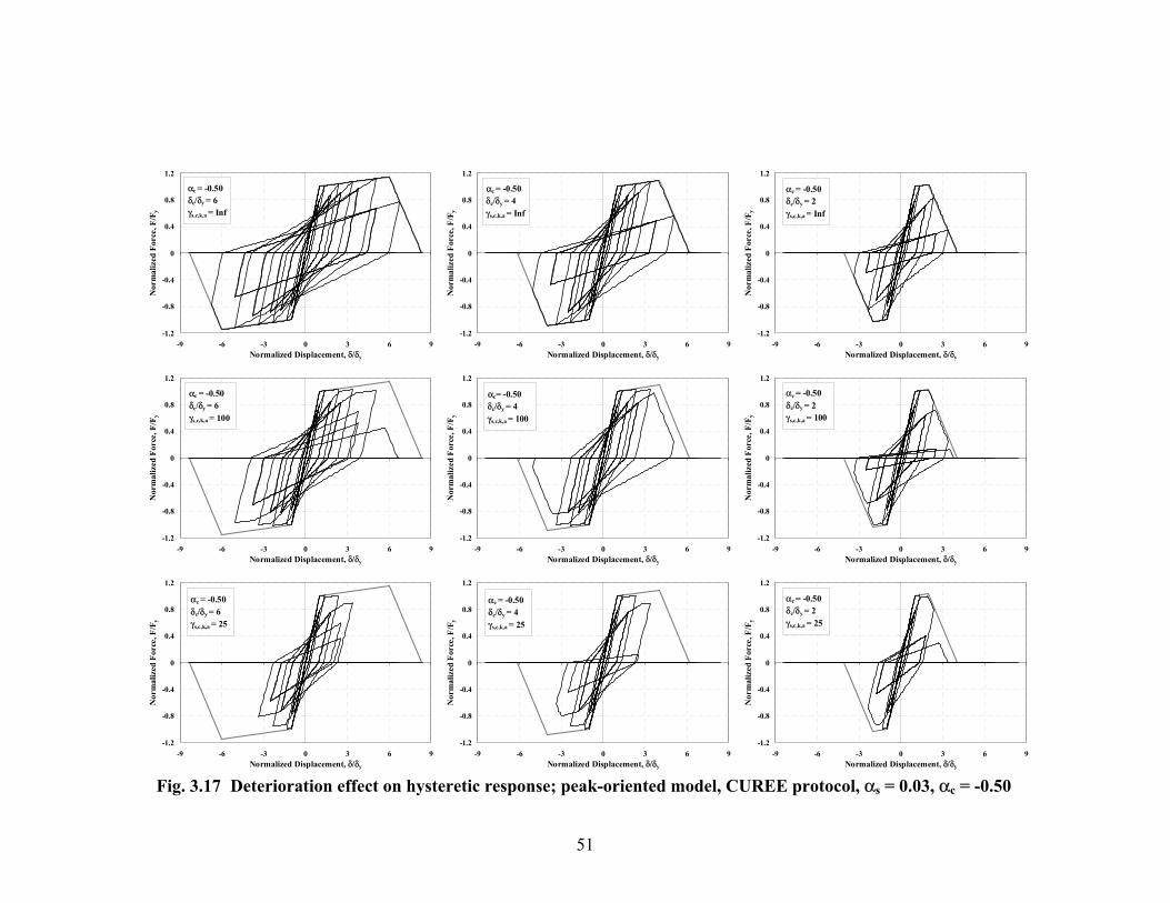
51

-1.2

-0.8

-0.4

0

0.4

0.8

1.2


Nor

mal

ized

For

ce, F

/Fy


-1.2

-0.8

-0.4

0

0.4

0.8

1.2


Nor

mal

ized

For

ce, F

/Fy


-1.2

-0.8

-0.4

0

0.4

0.8

1.2


Nor

mal

ized

For

ce, F

/Fy


-1.2

-0.8

-0.4

0

0.4

0.8

1.2


Nor

mal

ized

For

ce, F

/Fy

αc = -0.50 δc/δy = 6 γs,c,k,a = 100

-1.2

-0.8

-0.4

0

0.4

0.8

1.2


Nor

mal

ized

For

ce, F

/Fy

αc= -0.50 δc/δy = 4 γs,c,k,a = 100

-1.2

-0.8

-0.4

0

0.4

0.8

1.2


Nor

mal

ized

For

ce, F

/Fy

αc = -0.50 δc/δy = 2 γs,c,k,a = 100

-1.2

-0.8

-0.4

0

0.4

0.8

1.2


Nor

mal

ized

For

ce, F

/Fy

αc = -0.50 δc/δy = 6 γs,c,k,a = 25

-1.2

-0.8

-0.4

0

0.4

0.8

1.2


Nor

mal

ized

For

ce, F

/Fy

αc = -0.50 δc/δy = 4 γs,c,k,a = 25

-1.2

-0.8

-0.4

0

0.4

0.8

1.2


Nor

mal

ized

For

ce, F

/Fy

αc = -0.50 δc/δy = 2 γs,c,k,a = 25

Fig. 3.17 Deterioration effect on hysteretic response; peak-oriented model, CUREE protocol, αs = 0.03, αc = -0.50

4 Collapse Assessment of SDOF Systems

4.1 INTRODUCTION

Even though the deterioration model described in Chapter 3 is a component model, in the SDOF

study it is assumed that the system response follows the same hysteresis and deterioration rules

as a representative component. Clearly this is a simplifying assumption, as it is idealistic to

assume that all components of a structural system have the same deterioration properties and

yield and deteriorate simultaneously. But such assumptions are often made when MDOF

structures are represented with SDOF systems.

Parameter studies on SDOF systems are easily implemented and help to identify the

system parameters that may have a negligible or dominant influence on MDOF structures. The

small computational effort needed to analyze SDOF systems permits the evaluation of a large

number of systems. In addition, the modification of a particular parameter generally has a larger

influence on SDOF systems than on MDOF structures. The latter structures usually have

elements yielding at different times and some of the elements never reach the inelastic range;

thus, their global stiffness matrix has smaller modifications than the corresponding stiffness of

SDOF systems.

In the past, a large number of studies have been carried out to evaluate the inelastic

seismic demands of SDOF systems. Seismic demands have been studied by means of constant

ductility inelastic displacement ratios (Miranda, 1993, 2000) or by means of strength reduction

factors for constant ductility (Nassar and Krawinkler, 1991; Rahnama and Krawinkler, 1993).

The latter study included the effect of strength and stiffness deterioration in hysteretic models

with bilinear backbone curves. The results indicated that strength deterioration may greatly affect

the response of SDOF systems, but the effects of unloading stiffness deterioration are relatively

small. Gupta and Kunnath (1998) extended the investigation of Rahnama and Krawinkler,

obtaining similar conclusions. However, these studies are based on systems without strength

deterioration of the backbone curve and do not address the collapse limit state. More recently,

54

Song and Pincheira (2000) studied the effect of stiffness and strength deterioration on the

maximum inelastic displacement of SDOF systems without including geometric nonlinearities.

They found that the displacement ratio between a deteriorating and non-deteriorating system

could be as large as two (especially in the short-period range) and that it varies significantly with

the deterioration rate and type of ground motion. They assumed that an SDOF system collapses

if its remaining strength is less than 10% of the yield strength. They reported that many systems

collapsed for one or more ground motions under low strength coefficients but they did not trace

this limit state for all the cases. Vamvatsikos (2002) carried out incremental dynamic analyses

(IDAs) for pinched hysteretic SDOF systems that included a negative post-capping stiffness and

residual strength but no cyclic deterioration. He detected that the cap displacement (δc, Fig. 4.1)

and the slope of the post-capping stiffness are the two parameters that most affect the

performance of medium-period-systems.

This chapter summarizes the results of a comprehensive parameter study on the collapse

of SDOF systems with deteriorating hysteresis properties. In SDOF systems collapse occurs

when the loading path is on the backbone curve (which may have deteriorated due to cyclic

deterioration) and the restoring force approaches zero (Fig. 4.1). This behavior may occur

because of the presence of a backbone curve branch with negative slope, a condition caused by

P-∆ effects and/or a negative post-capping stiffness branch. Note that a backbone curve with

only positive stiffness branches may also lead to collapse if cyclic strength deterioration is

sufficiently large to exhaust the available energy-dissipation capacity.

In this part of the study, collapse is evaluated for a large number of SDOF systems

subjected to a set of 40 ground motions. Statistics on the collapse capacity take into account the

record to record variability. The effects of various system parameters are evaluated by comparing

median collapse capacities of systems that have the same characteristics except for discrete

variations in the studied parameter.

4.2 SYSTEMS AND GROUND MOTIONS CONSIDERED IN PARAMETER STUDY

The SDOF systems of the parameter study have common features, which include the same

strain-hardening stiffness ratio (αs = 0.03) and the same 20 elastic periods to be analyzed for

each hysteretic case. Also, most of the systems are subjected to the same set of 40 GMs, although

55

a limited study is carried out for two additional sets that present different frequency content

characteristics (Sections 4.4.6–4.4.7).

Collapse capacities are obtained in the fashion described in Section 2.3. The systems are

analyzed under increasing relative intensity values to obtain (Sa/g)/η - EDP relationships. The

smallest relative intensity represents elastic behavior, i.e., (Sa/g)/η = 1. Thus, previous to

carrying out the dynamic analyses, the spectral acceleration at the period of the system or the

yielding strength is scaled to obtain this relative intensity. For subsequent analyses the relative

intensity is increased until the response of the system becomes unstable, which means that the

(Sa/g)/η - EDP curve becomes flat (zero slope). The assessment of collapse is based not on EDPs

but on the relative intensity of the system when collapse occurs. This relative intensity is referred

as “collapse capacity,” (Sa,c/g)/η. Statistics are carried out for collapse capacity at each period.

The resulting median (Sa,c/g)/η - T curves are called “median collapse capacity spectra,” and are

the main tool to evaluate collapse capacity and the influence of system parameters on collapse. In

addition, the generated (Sa/g)/η - EDP curves are utilized to investigate the effects of

deterioration prior to collapse.

In order to reduce the number of combinations to be analyzed, the study is divided into

two parts:

(1) Primary Parameter Study. Several discrete values are considered for the parameters of

most interest and analyses are carried out for all possible combinations. The

combinations are needed because the effect of a particular parameter on the response of

the system may depend strongly on the relative value of the rest of the parameters.

(2) Secondary Parameter Study. This considers parameters that could have an influence on

the response but are not included in the main parameter study; only representative

systems are evaluated.

4.2.1 Parameters Evaluated in Primary Parameter Study

This part of the study focuses on the five system parameters described below, each of them with

three or four discrete values. A large number of nonlinear analyses are generated because all

these parameters are combined, and each combination includes 20 natural periods and 40 GMs,

in which the relative intensity is increased until collapse is reached. To limit the number of

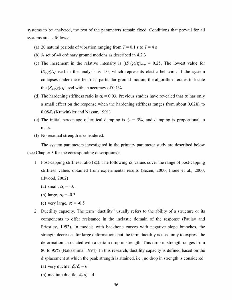
56

systems to be analyzed, the rest of the parameters remain fixed. Conditions that prevail for all

systems are as follows:

(a) 20 natural periods of vibration ranging from T = 0.1 s to T = 4 s

(b) A set of 40 ordinary ground motions as described in 4.2.3

(c) The increment in the relative intensity is [(Sa/g)/η]step = 0.25. The lowest value for

(Sa/g)/η used in the analysis is 1.0, which represents elastic behavior. If the system

collapses under the effect of a particular ground motion, the algorithm iterates to locate

the (Sa,c/g)/η level with an accuracy of 0.1%.

(d) The hardening stiffness ratio is αs = 0.03. Previous studies have revealed that αs has only

a small effect on the response when the hardening stiffness ranges from about 0.02Ke to

0.08Ke (Krawinkler and Nassar, 1991).

(e) The initial percentage of critical damping is ξo = 5%, and damping is proportional to

mass.

(f) No residual strength is considered.

The system parameters investigated in the primary parameter study are described below

(see Chapter 3 for the corresponding descriptions):

1. Post-capping stiffness ratio (αc). The following αc values cover the range of post-capping

stiffness values obtained from experimental results (Sezen, 2000; Inoue et al., 2000;

Elwood, 2002)

(a) small, αc = -0.1

(b) large, αc = -0.3

(c) very large, αc = -0.5

2. Ductility capacity. The term “ductility” usually refers to the ability of a structure or its

components to offer resistance in the inelastic domain of the response (Paulay and

Priestley, 1992). In models with backbone curves with negative slope branches, the

strength decreases for large deformations but the term ductility is used only to express the

deformation associated with a certain drop in strength. This drop in strength ranges from

80 to 95% (Nakashima, 1994). In this research, ductility capacity is defined based on the

displacement at which the peak strength is attained, i.e., no drop in strength is considered.

(a) very ductile, δc/δy = 6

(b) medium ductile, δc/δy = 4

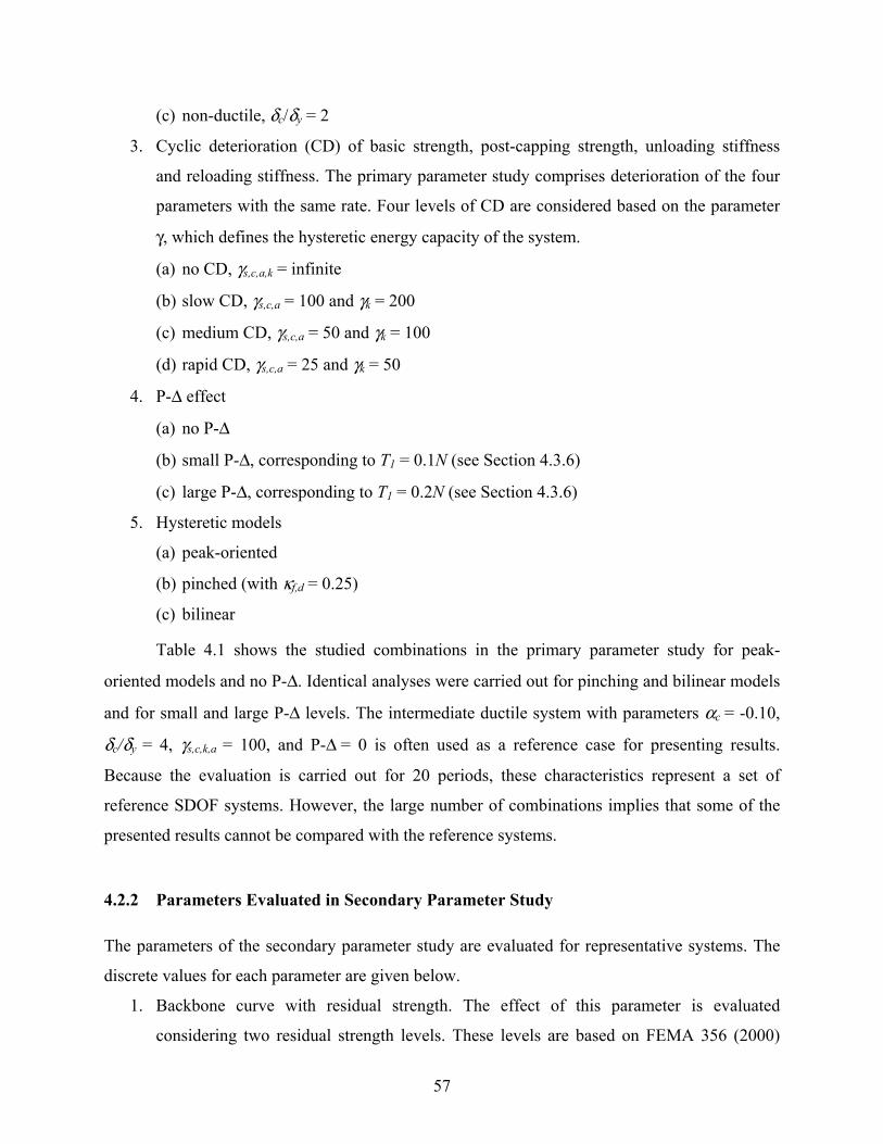
57

(c) non-ductile, δc/δy = 2

3. Cyclic deterioration (CD) of basic strength, post-capping strength, unloading stiffness

and reloading stiffness. The primary parameter study comprises deterioration of the four

parameters with the same rate. Four levels of CD are considered based on the parameter

γ, which defines the hysteretic energy capacity of the system.

(a) no CD, γs,c,a,k = infinite

(b) slow CD, γs,c,a = 100 and γk = 200

(c) medium CD, γs,c,a = 50 and γk = 100

(d) rapid CD, γs,c,a = 25 and γk = 50

4. P-∆ effect

(a) no P-∆

(b) small P-∆, corresponding to T1 = 0.1N (see Section 4.3.6)

(c) large P-∆, corresponding to T1 = 0.2N (see Section 4.3.6)

5. Hysteretic models

(a) peak-oriented

(b) pinched (with κf,d = 0.25)

(c) bilinear

Table 4.1 shows the studied combinations in the primary parameter study for peak-

oriented models and no P-∆. Identical analyses were carried out for pinching and bilinear models

and for small and large P-∆ levels. The intermediate ductile system with parameters αc = -0.10,

δc/δy = 4, γs,c,k,a = 100, and P-∆ = 0 is often used as a reference case for presenting results.

Because the evaluation is carried out for 20 periods, these characteristics represent a set of

reference SDOF systems. However, the large number of combinations implies that some of the

presented results cannot be compared with the reference systems.

4.2.2 Parameters Evaluated in Secondary Parameter Study

The parameters of the secondary parameter study are evaluated for representative systems. The

discrete values for each parameter are given below.

1. Backbone curve with residual strength. The effect of this parameter is evaluated

considering two residual strength levels. These levels are based on FEMA 356 (2000)

58

recommendations to specify deformation ranges in which the component responds with

substantially reduced strength:

(a) λ = 0.2 Fy

(b) λ = 0.4 Fy

2. Effect of individual cyclic deterioration modes. In the primary parameter study, the same

rate of deterioration is considered for all four modes of cyclic deterioration. In the

secondary parameter study the effect of individual deterioration modes on collapse

capacity is isolated.

3. Level of pinching in pinched hysteretic model: The effect on collapse capacity is

evaluated for the following cases:

(a) κf,d = 0.25 (from primary parameter analysis)

(b) κf,d = 0.5

(c) κf,d = 0.75

4. Damping of the system (ξ). The primary parameter study considers systems with mass

proportional damping and initial (or elastic) percentage of critical damping ξo = 5%.

This percentage of critical damping is applied to the system without P-∆ effects. In this

work, the effect on collapse capacity is studied for the following cases:

(a) mass proportional damping for ξo = 5% and 10%

(b) stiffness proportional damping for ξo = 5% and 10%

(c) mixed formulation for ξo = 5% and 10%, preserving ξo value in the inelastic range.

5. Deteriorating systems subjected to near-fault ground motion (NFGM) records.

6. Deteriorating systems subjected to long-duration records.

4.2.3 Set of Ground Motion Records LMSR-N

In this study, most of the structural systems are subjected to a set of 40 “ordinary” ground

motions recorded in California (LMSR-N, large magnitude small distance-new7). The records do

not exhibit pulse-type near-fault characteristics and are recorded on stiff soil or soft rock,

corresponding to soil type D according to NEHRP (FEMA-356, 2002). The source-to-site

distance ranges from 13–40 km. and the moment magnitude from 6.5–6.9 (Table 4.2).

7 The GM selection process for this bin is discussed in Medina (2002).

59

The selected intensity measure, IM, is the 5% linear elastic spectral acceleration at the

period of the SDOF systems, Sa(T). This IM has the advantage that seismic hazard data for Sa are

readily available; however, there are drawbacks to the use of a single scalar IM, and alternatives

are being investigated (Cordova et al., 2000; Luco, 2002). The use of Sa as IM implies that all the

ground motions are scaled to a common Sa at the elastic period of the SDOF system. Thus, the

frequency content of the ground motion cannot be considered explicitly. The large dispersion in

spectral accelerations due to the different frequency content of the selected ground motions is

illustrated in Figure 4.2, in which the records of set LSMR-N are scaled to have the same

spectral acceleration at T = 0.9 s. Figure 4.2b shows the dispersion in terms of the standard

deviation of the log of Sa for the scaled spectra, aSlnσ , which is small only in the vicinity of T =

0.9 s. The dispersion increases with period, and response predictions may exhibit significant

scatter depending on the extent of inelasticity, which leads to period elongation.

The use of a single set of GMs for most of this study is partly justified by previous

studies showing that the inelastic response of SDOF and MDOF systems is not affected greatly

by earthquake magnitude and distance to the source—except for near-fault regions (Shome,

1999; Miranda, 2000; Medina, 2002; Jalayer, 2003).

Regarding the size of the set of GMs, the uncertainty associated with the estimated EDPs

and collapse capacities may be quantified as a function of the number of data points evaluated in

the form of confidence levels. The use of a set of 40 GMs provides estimates of the median that

are within a one-sigma confidence band of 10% as long as the standard deviation of the natural

log of the collapse capacities or EDPs is less than 63.01.0 =N , where N is the number of

records (Medina, 2002).

1.1 4.3 RESULTS OF PRIMARY PARAMETER STUDY

Most of the results discussed and illustrated in this chapter represent statistical values,

particularly medians. “Counted statistics” is used to obtain the first moments of EDPs given

(Sa/g)/η, and “computed statistics” is utilized for collapse capacities (Appendix A). The EDPs

used in the SDOF study are δmax/Sd, δmax/δy and occasionally normalized hysteretic energy

dissipation, NHE. The presented results are for peak-oriented hysteresis models unless stated

differently.

60

To identify the effect of each parameter on the response, the results are grouped in sets of

similar systems that present a variation of specific parameters. Because none of the parameters

can be evaluated independently of the others, the variation of parameters is carried out for

systems with different characteristics. For instance, the effect of αc on (Sa,c/g)/η is quantified for

different types of hysteretic models, δc/δy’s, γ’s and P-∆ levels (see Table 4.1). The following

sections summarize the salient findings of this study.

4.3.1 Effect of Deterioration on EDPs Prior to Collapse

Although the main objective of this study is collapse capacity assessment, the evaluation of the

response prior to collapse provides valuable information about the effect of various deteriorating

models on EDPs. The main objectives of this section are (a) to quantify the increment in the

response when deteriorating systems are used instead of non-deteriorating ones; and (b) to

determine the intensity levels at which the response of deteriorating systems starts to deviate

from that of non-deteriorating systems. In this investigation the term “non-deteriorating” is used

for systems without any type of material deterioration, although they could include P-∆ effects.

The results presented in this section are grouped according to variations of specific parameters

and are for systems with T = 0.2, 0.9, and 3.6 s, corresponding to short-, medium-, and long-

period systems, respectively.

Effect of Cyclic Deterioration (CD) on EDPs. Figure 4.3 shows (Sa/g)/η - EDP curves

for a system with T = 0.9 s, αc = -0.10, δc/δy = 4, P-∆ = 0, and different γs,c,k,a values for

deteriorating systems. Curves for a non-deteriorating system with the same elastic and hardening

stiffness and for the “equal displacement rule” are also included. For low relative intensities the

equal displacement rule is approximately valid for all systems, i.e., for 4/)/( ≤= ηgSR a , the

ductility and relative intensity have approximately the same value, i.e., yR δδ /max≈ .

Comparisons of the response between these systems indicate that the effect of CD is small (at

most 10–15%) before the ductility capacity is reached (δmax/δy = δc/δy = 4). The curves start to

show large deviations from the non-deteriorating system once this threshold is surpassed. This

can be observed best in Figure 4.3c by applying the equal displacement rule. All three figures

clearly show the benefit being derived from an increase in the energy-dissipation capacity

(increase in γ’s) of the SDOF system—for a system with αc = -0.10 and δc/δy = 4.

61

The results for very short and long-period systems with the same properties are presented

in Figures 4.4 and 4.5, respectively. For systems with T = 0.2 s and rapid CD, a clear deviation

from the non-deteriorating system is evident long before the ductility capacity is reached. On the

other hand, for long-period systems the effect of CD is relatively small even for values of δmax/δy

much greater than the ductility capacity of 4. The above trends are similar for systems including

P-∆ effects.

Effect of Post-Capping Stiffness on EDPs. In systems that are identical except for the

post-capping stiffness branch, the EDPs are the same for displacements less than cδ . For

medium-period systems with a flat post-capping stiffness (αc = -0.10), the relative intensity of

the system may be increased significantly after this displacement threshold is surpassed (Fig.

4.6). However, for αc = -0.30 and –0.50, the additional relative intensity that the system can

sustain once δmax/δy > δc/δy is small.

The last observation holds true also for short- and long-period systems (Fig. 4.7), leading

to the conclusion that only relatively small improvement in response can be obtained once the

ductility capacity δc/δy is reached, unless the post-capping stiffness is relatively flat, i.e., it makes

little difference whether αc is –0.30 or –0.50. Only for αc = -0.1 a clear improvement is observed

for all systems. As Figure 4.7b shows, the improvement beyond δmax/δy = δc/δy = 4, in terms of

additional displacement capacity and additional “intensity capacity,” is particularly large for

long-period systems. P-∆ effects could modify this conclusion, especially for long-period

systems where large instability coefficients usually have to be considered (see Section 4.3.6).

Effect of Ductility Capacity on EDPs. Figures 4.8–4.9 present median (Sa/g)/η - EDP

curves for identical systems except for the ductility capacity value. Because CD is not included,

the curves for deteriorating and non-deteriorating systems are identical up to δmax/δy = δc/δy. All

the presented systems have a flat post-capping stiffness, and for this reason all systems exhibit a

significant increase in displacement and intensity beyond that associated with the ductility

capacity.

4.3.2 General Trends in Collapse Capacity Spectra, (Sa,c/g)/η - T

Collapse capacity spectra are used in the following sections to evaluate the effects of the system

parameters that greatly affect collapse. To obtain an idea of the possible collapse capacity values,

62

Figure 4.10 shows the range of median collapse capacity spectra for deteriorating peak-oriented

models including all possible combinations of the primary parameter study (Table 4.1). Each

median collapse capacity spectrum refers to the estimation of the geometric mean of the 40

individual collapse capacity spectra, which are obtained by subjecting a particular system to the

records of the set LMSR-N (Section 2.3.4).

Figure 4.11 presents median collapse capacity spectra for representative systems, as well

as the ratios of collapse capacities with respect to the most ductile system of the primary

parameter study (αc = -0.1, δc/δy = 6, γs,c,k,a = Inf, P-∆ = 0). Note that collapse capacities of the

reference case (αc = -0.1, δc/δy = 4, γs,c,k,a = 100, P-∆ = 0) are about 30% smaller that those of the

most ductile system. Collapse capacities of the less ductile system are up to five times smaller

than those of the most ductile one. However, from this figure alone it is difficult to identify the

parameters that most influence the response of the system because several of them are modified

at once. Thus, the effect of each individual parameter is isolated in the following sections. From

here on, when ratios of collapse capacities are presented, they are always obtained by using the

most ductile case of the specific parameter variation as the base case.

A basic conclusion from the primary parameter study is that the effect of any one

parameter on the collapse capacity is dictated in part by the rest of the parameters. In this

investigation, the interdependence is evaluated for the five parameters of the primary parameter

study. For instance, the effect of αc on collapse capacity is assessed for systems with different

values of δc/δy, γ and P-∆ effect. The results are presented for systems with peak-oriented

hysteretic models except when the effects of different hysteretic models are evaluated.

4.3.3 Effect of Post-Capping Stiffness on Collapse Capacity

The dependence of the median (Sa,c/g)/η on αc is shown in Figure 4.12 for periods between 0.1–

1.0 s. The system corresponds to the reference case if αc = -0.10. Except for very short-period

systems, the collapse capacities are very sensitive to variations of αc when this parameter is

small. Collapse capacities increase exponentially when αc approaches zero. For large αc values,

(Sa,c/g)/η stabilizes at the relative intensity that the system can develop when the maximum

displacement is equal to δc.

Figure 4.13 presents the effect of αc on the median (Sa,c/g)/η for a set of systems with

δc/δy = 4, γs,c,k,a = infinite, and no P-∆ effects. Median collapse capacity curves and ratios with

63

respect to the most ductile system of this set are presented. Except for very short-period systems,

a large decrease in collapse capacity is observed for systems with αc = -0.30 with respect to

systems with αc = –0.10. Any further increase in negative slope beyond αc = -0.30 has a small

effect because collapse occurs soon after δc has been reached. The effect of αc on the collapse

capacity increases for systems with longer periods when P-∆ = 0.

The effect of αc is even larger for systems with smaller δc/δy. Figure 4.14 presents the

effect of αc for the same set of systems of Figure 4.13 except for δc/δy = 2. As can be seen, the

collapse capacities are significantly reduced compared to δc/δy = 4; a reduction that is

proportionally larger for systems with large αc, leading to smaller collapse capacity ratios. That

is to say, the effect of αc on collapse capacity is magnified in systems with small ductility

capacity because proportionally a larger fraction of the relative intensity is developed after δc is

surpassed. If P-∆ effects are included, collapse capacities are greatly reduced for medium- and

long-period systems where the stability coefficient is larger. Compare Figures 4.15–4.16 with

Figures 4.13–4.14, respectively. As observed, the effect of αc still is relevant and the ductility

capacity parameter still has an important influence.

The influence of CD on the effect of αc on collapse capacity is illustrated in Figure 4.17,

which shows collapse capacities for the systems of Figure 4.13 but including medium CD (γ =

50). Larger collapse capacity ratios are observed because CD reduces in a larger proportion the

collapse capacities of systems with small αc. That is to say, the effect of αc on collapse capacity

is reduced for systems with large CD.

Collapse capacities of bilinear models are smaller than those of the peak-oriented models

(compare Figs. 4.13–4.18). The main reason is that the negative post-capping stiffness affects the

bilinear model more because of the “ratcheting” effect (Section 4.3.7). In bilinear models the

effect of αc on (Sa,c/g)/η is smaller in the short-period range compared with the peak-oriented

one. This occurs because of the large decrease in collapse capacity for systems with flat post-

capping stiffness; compare Figures 4.13 and 4.18. Note that collapse capacities for bilinear

models with αc = -0.30 and αc = -0.50 are practically the same.

The dispersion of collapse capacities is presented in Figure 4.19 for representative

systems, using the standard deviation of the log of (Sa,c/g)/η. In general the dispersion is larger

for more ductile systems, as the one with αc = -0.10 and no P-∆ effects (4.19a). P-∆ effects

slightly reduce the dispersion because they make the system less “ductile.” The largest standard

64

deviation is at most about 0.60, which means that the estimates of the median are within a one-

sigma confidence band of 10% because the number of records used is 40.

Summarizing, the effect of αc may modify the collapse capacity by more than 100%,

particularly for long-period systems with no P-∆ effects. The magnitude of this effect depends

not only on the “ductility” of the system but also on the parameters that induce such behavior.

For instance, systems are less ductile when δc/δy is smaller, but the effect of αc becomes larger

because a larger proportion of the nonlinear response occurs after δc has been reached. On the

other hand, systems are more ductile when CD is slower, and in these systems the effect of αc is

more important.

4.3.4 Effect of Ductility Capacity on Collapse Capacity

The dependence of the median (Sa,c/g)/η on δc/δy is illustrated in Figure 4.20. If δc/δy = 4, the

SDOF system is equivalent to the reference system. The δc/δy -(Sa,c/g)/η relationship is close to

linear for all periods. For very short periods the corresponding curve is close to a horizontal line,

indicating that the collapse capacity is not affected much by variations in δc/δy, as in the case of

αc.

Figure 4.21 shows the effect of δc/δy on systems with αc = -0.10, γ = infinite, and P-∆ = 0.

Median collapse capacity curves as well as the ratios with respect to the most ductile system are

presented. Observe that except for very short periods, the median collapse capacity is essentially

period independent (Fig. 4.21b). The effect of δc/δy on collapse capacities is significant, but

much less than the ratio of ductility capacities. The main reason for the relatively small effect is

the fact that because of the flat post-capping slope (αc = 0.1) all systems exhibit a significant

intensity increase beyond that associated with δc. Figure 4.22 shows the same information but

using systems with αc = -0.30. The steeper post-capping slope significantly reduces the collapse

capacities, but also magnifies the effect of δc/δy. Collapse ratios close to 0.40 are observed. The

effect of δc/δy increases for larger αc values because collapse occurs relatively soon after δc is

reached.

Collapse capacities are reduced if P-∆ effects are included, but collapse capacity ratios

still tend to be period independent and with values similar to those obtained for systems with no

P-∆ effects (compare Figs. 4.23 and 4.21). The effect of δc/δy on the collapse capacity for

65

systems with medium CD (γ = 50) is shown in Figure 4.24, which can be compared with the

system with no CD (Fig. 4.21). The effect of δc/δy on the collapse capacity becomes relatively

small for systems with significant CD.

Figure 4.25 shows similar information to that of Figure 4.21 but using systems with a

bilinear model. Compared with peak-oriented models, the collapse capacities are smaller but the

effect of δc/δy is larger. As will be explained in Section 4.3.7, bilinear models are more affected

by the presence of a branch with negative stiffness. Therefore, the effect of reducing δc/δy has a

larger effect on the collapse capacity because δc is surpassed at earlier stages of nonlinear

behavior.

Figure 4.26 presents a measure of dispersion for systems having different δc/δy. There is

no significant difference or clear trend among the dispersion curves for systems with large and

small ductility capacity. This suggests that dispersion largely depends on the post-capping

stiffness parameter rather than the ductility capacity. P-∆ effects reduce the standard deviation of

the log of the data, especially for long-period systems.

4.3.5 Effect of Cyclic Deterioration on Collapse Capacity

Cyclic deterioration is assumed to be proportional to the energy-dissipation capacity of the

system, defined by the parameter γ. The dependence of the median (Sa,c/g)/η on γ is illustrated in

Figure 4.27. If γs,c,k,a = 100, the system corresponds to the reference system. The systems of

Figure 4.27 have a negative post-capping branch (αc = -0.10) that eventually leads to collapse

even if CD is not present. As the figure shows, for these systems CD has an appreciable effect on

the collapse capacity only if γ is on the order of 100 or smaller.

Figure 4.28 presents the effect of CD on collapse capacities for a set of systems with

δc/δy = 4 and αc = -0.10. Except for very short periods, the collapse capacity ratios are in essence

period independent, with values as small as 0.5 (this large effect is observed only for αc = -0.10).

The expectation might be that CD has a larger effect for short-period systems because of the

larger number of inelastic cycles. As Figure 4.28b shows, this is not true—for two reasons.

First, for short-period systems the effects of all system parameters on the collapse capacity are

small because of the dominant displacement amplification effect for inelastic systems. And

second, for systems without CD the normalized hysteretic energy (NHE) demands are much

66

higher for short-period systems than for medium- and long-period systems, but the demands

become less period sensitive for systems with cyclic deterioration (Fig. 4.29). Thus, the

displacement amplification effect dominates over the effect of cyclic deterioration.

Figure 4.30 presents the same information as Figure 4.28, but for systems with small

ductility capacity. The patterns are the same but the effect of CD on the collapse capacity is

smaller for systems with small ductility capacity because these reach collapse faster and have

less time to dissipate hysteretic energy. Figure 4.31 shows the effect of CD on the collapse

capacity for systems with αc = -0.30, which again can be compared with Figure 4.28. Once

again, the presence of a parameter that reduces the collapse displacement in the system reduces

the effect of CD on the collapse capacity because the number of inelastic cycles is decreased.

The effect of CD on the collapse capacity is much reduced in medium- and long-period

systems that include P-∆ effects. Figure 4.32 presents the results for the set of systems of Figure

4.28 but including small P-∆ effects. Collapse capacity ratios for different CD values approach

unity for long-period systems. This indicates that for such systems P-∆ effects dominate over the

effect of CD on collapse capacity.

The effect of CD on the collapse capacity for bilinear models is illustrated in Figure 4.33,

which can be compared with Figure 4.28. The collapse capacity ratios are about the same for

bilinear and peak-oriented models, but the median collapse capacities are clearly smaller for the

bilinear model for reasons that will be discussed in Section 4.3.7.

The dispersion for similar systems with different rates of CD (Fig. 4.34) indicates that the

standard deviation of the log of the data decreases somewhat with an increase in CD.

It is concluded that the effect of CD on the collapse capacity always increases when any

of the other system parameters cause a more ductile response. This is a clear pattern that was not

detected in other parameters. However, the effect of CD on the collapse capacity is smaller than

that caused by large variations in the backbone curve parameters and, for long-period systems,

by P-∆ effects.

4.3.6 Effect of P-∆ on Collapse Capacity

Traditionally, P-∆ effects are quantified by means of the elastic stability coefficient (Sun et al.,

1973; Bernal, 1986). This coefficient can be associated with a rotation of the original backbone

curve (Fig. 4.1) and could have a very significant effect on the behavior of the system (Vian and

67

Bruneau, 2001). In fact, systems without material deterioration may collapse if P-∆ effects are

sufficiently large. The stability coefficient is defined as:

hFW

khP

y

yδθ == (4.1)

where P is the vertical acting load, which here is assumed to be equal to the weight of the SDOF

system, gmW /= ; ke is the elastic stiffness, yye Fk δ/= ; and h is the height of the system. For

SDOF systems, the stability coefficient can be expressed in a simplified form by taking into

account that:

kmT π2= (4.2)

After substituting Equation (4.2) into (4.1) and considering g = 981 cm/s2, the elastic

stability coefficient can be defined as a function of the period and the height (in centimeters) of

the SDOF system:

hT 225=θ (4.3)

his equation helps to set practical limits for θ. For instance, if T = 1.0 s and the height of the

system is 244 cm ( ≈ 8′); then θ ≈ 0.10, which is a large coefficient for a system with T = 1.0 s.

The reason for the large value is the small height of 244 cm, which is not representative for a

medium-period system. Moreover, the number of parameters influencing P-∆ effect is increased

if SDOF systems are used as simplifications of MDOF structures, i.e., the number of stories,

assumed loading pattern, deflected shape of the MDOF structure, irregularities in height or plan,

distribution of vertical load, etc. (Bernal, 1992). As discussed in Chapter 5, P-∆ effects for

equivalent SDOF systems should be derived from both elastic and inelastic stability coefficients

obtained from global pushover analysis of the MDOF structure.

Thus, stability coefficients for equivalent SDOF systems should be calculated for each

specific structure. In order to establish general trends, in this section the effect of P-∆ on

collapse capacity is evaluated by using the elastic stability coefficients corresponding to the first

story of the generic frames used in Chapter 5. These frames have 3, 6, 9, 12, 15, and 18 stories,

and for a given number of stories a stiff and a flexible model are designed by targeting a

fundamental period of vibration of T1 = 0.1N and T1 = 0.2N, respectively. For these frames, the

elastic first-story stability coefficient can be estimated as 0.0178T1 and 0.0356T1 for the stiff and

68

flexible models, respectively. Consequently, the following three P-∆ levels are used here for

each period:

(a) no P-∆, θ = 0.0

(b) small P-∆, θ = 0.0178T1 (stiff system, T1 = 0.1N)

(c) large P-∆, θ = 0.0356T1 (flexible system, T1 = 0.2N)

Figure 4.35 shows the stability coefficients for each P-∆ level as a function of the period

of the system. The assigned levels are used only to identify general patterns.

The effect of P-∆ on collapse capacities is shown in Figure 4.36 for an intermediate

ductile SDOF system. As observed, the P-∆ effect produces the largest modification of collapse

capacities in the long-period range. The effect is largest in this range because of the large

stability coefficients that overcome the 3% strain hardening of the second branch of the

backbone curve and cause an effective negative tangent stiffness as soon as the yield

displacement is reached. Note that in the long-period range the collapse capacities for systems

with small and large P-∆ effects are similar. At this range, the strain-hardening slope has become

negative for both P-∆ levels (Fig. 4.35). Therefore, merely the presence of a branch with

negative stiffness greatly accelerates collapse, regardless of the value of the slope (Bernal, 1986;

Gupta and Krawinkler, 2001).

Figure 4.37 shows the same information as Figure 4.36, but for systems with a small

ductility capacity. The collapse capacity is reduced, but the collapse capacity ratios are similar

for the two cases, indicating that ductility capacity does not greatly modify the effect of P-∆ on

collapse capacity.

Figure 4.38 presents collapse capacities for the systems of Figure 4.36, but using a large

αc value. Comparing these two figures in the long-period range, it is seen that the effect of a

large αc value is large for systems without P-∆ effect but small for systems with P-∆. The reason

is that the backbone curve (without P-∆ effects) already has a steep negative αc; thus, the

increment in the negative stiffness due to the inclusion of P-∆ effects is small compared with

systems with a small αc.

The effect of P-∆ on the collapse capacity is marginally affected by the CD rate of the

system, as revealed by a comparison of collapse capacities and corresponding ratios for systems

with medium CD of Figure 4.39 with those of Figure 4.36.

69

Figure 4.40 displays collapse capacities for bilinear models. Comparing these results with

those of Figure 4.36 (peak-oriented models), it is clear that the negative stiffness of the backbone

curve has a larger effect on the deterioration of bilinear models. The following section provides

more details in this respect.

4.3.7 Effect of Type of Hysteretic Model on Collapse Capacity

This section is aimed to test the effect of the type of hysteretic model on the collapse capacity,

given that former sections have focused on results for peak-oriented models. To obtain a general

idea of collapse capacities when using different hysteretic models, Figure 4.41a shows median

(Sa,c/g)/η ratios for pinching over peak-oriented models for all the systems that do not include P-

∆ effects. The median collapse capacity of pinching models is larger than that of peak-oriented

models, except in the short-period range. Figure 4.41b shows median collapse capacity ratios for

bilinear over peak-oriented models without P-∆ effects. In this case the pattern reverses and the

difference between collapse capacities is more pronounced.

Therefore, in the medium- and long-period ranges, collapse capacities are largest for

pinching models, followed by those for peak-oriented and bilinear models (the same trends in the

response of EDPs are obtained by Foutch, 1996). In the short-period range the behavior is

reversed and the bilinear models have the largest collapse capacities. In the case of systems with

P-∆ effects, the patterns for collapse capacities are preserved but the ratios are closer to 1.0,

particularly for long-period systems (Fig. 4.42). The ratios are studied in more detail below to

understand what system characteristics produce smaller or larger ratios in the former figures.

Figure 4.43 presents bilinear over peak-oriented collapse capacity ratios for two systems

with extreme backbone curve features. One of the systems has a small ductility capacity and a

flat post-capping stiffness (δc/δy = 2, αc = -0.1), whereas the other has δc/δy = 6 and αc = -0.3.

The latter system8 has large ductility capacity but collapse occurs soon after δc is surpassed

because of the steep post-capping stiffness. That is to say, most of the collapse capacity is

developed previous to the attainment of δc, i.e., in a range in which the hysteretic model behaves

in the same way as that of a non-deteriorating system. For this system the ratios are closer to one,

meaning that the collapse capacity is similar for both hysteretic models. This is in agreement 8 These systems are useful to understand the patterns of Figure 4.43 but they are not usually expected in real components because of the combination of very ductile and non-ductile parameters in the same backbone curve.

70

with the results for EDPs obtained by Foutch (1998) and the results for R-factors for constant

ductility obtained by Nassar and Krawinkler (1991).

In the systems with small ductility capacity (δc/δy = 2) the post-capping stiffness is

reached relatively soon and because of the small post-capping stiffness (αc = -0.1) a large part of

the collapse capacity of the system is developed after δc is surpassed. In these systems, the

bilinear over peak-oriented collapse capacity ratios are as low as 0.6, indicating that collapse

capacity for bilinear models is substantially smaller than that of peak-oriented models. One

reason, and probably the primary one, is the presence of a branch on the backbone curve with

negative tangent stiffness, which produces a ratcheting effect for bilinear systems that tends to

cause a faster collapse. However, a negative post-yielding slope may be originated by other

factors. For instance, Rahnama and Krawinkler (1993) have concluded that peak-oriented models

behave better than bilinear ones if large P-∆ effects are present that produce a negative post-

yielding slope. The peak-oriented model spends most of its time in “inner” loops in which the

loadings stiffness is always positive, rather than on the backbone curve where the negative

tangent stiffness leads to drifting of the displacement response.

Figure 4.44 present the bilinear over peak-oriented collapse capacity ratios for several

combinations of αc and δc/δy. These graphs confirm that the steeper the post-capping slope, the

closer the collapse capacities for both hysteretic models.

Figure 4.45 shows bilinear over peak-oriented collapse capacity ratios for systems with

small αc, medium or small δc/δy, and different rates of CD. The difference in collapse capacities

is larger for systems with less cyclic deterioration. Therefore, the effect of cyclic deterioration is

smaller in systems with bilinear models.

4.3.8 Increment in Collapse Capacity after Cap Displacement, δc, is Reached

Traditionally, guidelines including inelastic behavior, such as FEMA 356, consider that collapse

of SDOF systems occurs almost immediately after the peak (cap) point in the backbone curve is

reached or, at most, when the strength on the backbone curve has decreased 20% with respect to

its peak value. This section aims to quantify the increase in collapse capacity after δc is reached.

In the first part, systems without P-∆ effects are studied. Figure 4.46 shows the median

ratio of collapse capacity over the intensity level at which the ductility capacity of the systems is

reached. As observed, the ratios increase for systems with longer period. The ratios of four

71

identical systems except for the CD rate are plotted in 4.46a. The ductility capacity of the

systems is δc/δy = 4. The ratios are larger for systems with less CD, which indicates that the effect

of CD on EDPs increases after δc is surpassed.

The ratios of 4.46b correspond to identical systems except for αc. For systems with a

steep post-capping slope, the increment in collapse capacity is small after δc is reached. But the

increment is very large for systems with a flat post-capping slope. Figure 4.46c presents systems

where the only parameter that is varied is the ductility capacity, and unlike former cases, the less

ductile the system (smaller δc/δy), the larger is the increase in collapse capacity 9. The reason is

that the displacement until collapse after surpassing the peak displacement (δf –δc) is

proportionally larger in systems with small δc/δy, particularly for flat post-capping slopes. This

can be interpreted as having a larger δf /δc ratio. For instance, the systems of Figure 4.46 have

ductility capacities of δc/δy = 2, 4, and 6, and δf /δc = 6.3, 3.8, and 3.0, respectively.

Consequently, the system with small δc/δy and small αc develops a large part of the collapse

capacity once the negative slope is reached.

If P-∆ is included the above ratios are greatly reduced because the P-∆ effects lead faster

to collapse when the slope of the backbone curve is negative, especially for long-period systems

where the P-∆ effect dominates. This is observed in Figure 4.47, which repeats the results of

Figure 4.46 but including small P-∆ effect. Figure 4.48 shows how the ratios decrease when the

same system (δc/δy = 4 and αc = -0.1) is subjected to increasing P-∆ levels.

In summary, for models with small αc collapse capacity may be underestimated by a

great amount by neglecting the capacity of the system that is developed after δc is reached. For

systems with large αc, the collapse capacities may be approximated with the relative intensity

developed when the peak displacement is reached.

4.4 RESULTS OF SECONDARY PARAMETER ANALYSIS

4.4.1 Effect of Residual Strength, λFy, on Collapse Capacity

The effect of residual strength, which is not included in the primary parameter study, is evaluated

in this section. Models with residual strength and no P-∆ effects do not collapse unless CD is

9 The ratios for this set of systems have collapse capacities over relative intensities calculated at different δc/δy’s, because this is the parameter that is being varied.

72

included and the hysteretic energy capacity is exhausted (Fig. 4.49a). When the system includes

P-∆ effects, the backbone curve rotates and collapse occurs if (Sa/g)/η is large enough to cause a

zero restoring force when the loading path is on the backbone curve (Fig. 4.49b).

The displacement at which collapse occurs depends on the geometry of the backbone

curve. Figure 4.50 presents displacements at collapse normalized by the yield displacement (δf

/δy) for backbone curves with different residual strengths. The ratios correspond to ductile and

non-ductile systems and include small P-∆ effects and no CD. As can be seen, the presence of

residual strength increases the normalized collapse displacement in a larger proportion for non-

ductile systems. Also, residual strength does not modify δf /δy ratios in long-period systems,

where the large P-∆ effect leads to collapse before the loading path reaches the residual branch.

Recognizing that the effect of residual strength is sensitive to the geometry of the

backbone curve, several analyses were performed for systems with small P-∆ effects and the

following parameters: δc/δy = 2, 4, 6 and αc = -0.10, -0.30. Residual strengths of λFy = 0.2Fy and

0.4Fy are selected in accordance with FEMA 356, which recommends the former value for most

of the beam-column elements in most structural materials. The residual strength of 0.4Fy is

included because FEMA recommends residual strength values as large as 0.4, 0.6, and even

0.75Fy for some elements, e.g., shear walls and RC infilled columns. The results discussed below

about the effect of residual strength on collapse capacity are for systems with small P-∆ effects

and are grouped according to the CD rate.

Residual Strength Effect of Systems without CD. Figures 4.51–4.52 present collapse

capacities for ductile and non-ductile systems with no CD. The addition of residual strength

increases collapse capacities only for systems of short and medium periods. The increase is

important only for non-ductile systems with λ = 0.4; for systems with λ = 0.2 the increment is

negligible for all the systems.

Residual Strength Effect of Systems with CD. Collapse capacities for the same systems

are presented in Figures 4.53–4.54, but considering a medium CD rate. In the very short-period

range (T < 0.3 sec) the inclusion of CD greatly reduces the collapse capacity of systems with

residual strength. Nonetheless, for short-period non-ductile systems including CD, the increment

in collapse capacity when λ = 0.4 can be as much as twice that of models without residual

strength (Fig. 4.54b). The reduction in collapse capacity is explained by observing that δmax /δy

ratios are greatly reduced in the short-period range when CD is included (Fig. 4.55).

73

Collapse Capacity Based on Pre-Established Collapse Displacement. As observed in

Figure 4.55a, hysteretic models with residual strength and no CD may have unreasonably large

displacements leading to unrealistic collapse capacities, especially in the short-period range. To

avoid this situation, a judgment-based maximum displacement is imposed, in which the collapse

displacement of the backbone curve with residual strength is at most 1.6 times the collapse

displacement of the backbone curve without residual strength, δf (λ>0) ≤ 1.6 δf (λ=0). This

displacement constraint produces reasonable δmax/δy ratios even when CD is not included (Fig.

4.56). Figure 4.57 presents the effect of residual strength on collapse capacity for systems with

the displacement restriction δf (λ>0) ≤ 1.6 δf (λ=0). These results can be compared with those of

Figures 4.51b and 4.52b. As observed, the maximum collapse capacity ratios are about 1.2 but

only for non-ductile systems with λ = 0.4. For systems with λ = 0.2 the effect of residual strength

on collapse capacity is negligible. Hence, residual strength does not affect significantly the collapse capacity of most

structural components when reasonable assumptions for λ and δf /δy ratios are made.

4.4.2 Effect of Individual Cyclic Deterioration Modes

The effect of CD on collapse capacity has been evaluated considering the same deterioration rate

for basic strength, post-capping strength, unloading stiffness, and accelerated reloading stiffness

deterioration. This section isolates the effect of each deterioration mode on collapse capacity, an

assumption that may not be realistic but is useful for identifying the CD modes that are more

relevant in the estimation of collapse capacity. For each analyzed deterioration mode the

corresponding parameter γ is varied, whereas the rest of the modes remain without deterioration.

Cyclic Basic Strength Deterioration. This deterioration mode produces translation of

the hardening branch toward the origin and deterioration of its slope (Section 3.3.2). The effect

of this deterioration mode can be very different for systems with and without post-capping

stiffness.

In systems without a post-capping branch collapse occurs when the hysteretic energy

capacity of the system is exhausted, which means that restoring strength is zero. To illustrate this

effect, Figure 4.58a presents the hysteretic response for a non-deteriorating system subjected to

the CUREE standard loading protocol (Gatto and Uang, 2002), whereas Figure 4.58b shows the

74

hysteretic response for the same system but with γs = 50. As can be seen, the hysteretic response

may be greatly modified when the only source of deterioration is cyclic basic strength

deterioration. Regarding the effect of γs on collapse capacity, Figure 4.59 shows collapse

capacities for similar systems without strength capping and different CD rates. The collapse

capacity ratios for the less ductile systems (γs = 25) can be as low as 0.40 with respect to systems

with slow CD10 (γs = 100), corroborating that CD effects increase in systems without a negative

branch in the backbone curve.

In systems with a post-capping branch the effect of cyclic basic strength deterioration is

substantially smaller due to the presence of additional sources of deterioration. This is observed

in Figure 4.60, which shows the hysteretic response for a system with δc/δy = 2 and αc = -0.10

subjected to the CUREE standard loading protocol. For Figure 4.60a, the only source of

deterioration is the negative post-capping stiffness, whereas Figure 4.60b also includes cyclic

basic strength deterioration. Note that although the hardening branch moves inwards, the

absolute value of cap displacement (δc) increases. The increase of δc implies that systems

including strength CD may have a better response than systems not including CD, when

subjected to ground motions. Figure 4.61 presents collapse capacity ratios for systems with a

peak-oriented model, δc/δy = 2 and αc = -0.10 and different rates of strength CD (the ratios are

taken with respect to the system with no CD). As observed, some ratios are larger than one,

indicating that when only strength CD is included, the effect of increasing the absolute value of

δc may overcome the effect of strength capping. The box on the bottom left corner of Figure 4.61

shows the collapse capacity ratios when the four CD modes are included.

The conclusion is that cyclic basic strength deterioration must be combined with cyclic

post-capping strength deterioration in order to accelerate collapse. Experimental results have

demonstrated that indeed both cyclic deterioration modes occur simultaneously.

Cyclic Post-Capping Strength Deterioration. This individual CD mode translates the

post-capping branch toward the origin (Section 3.3.3). To illustrate the magnitude of this effect,

Figure 4.62a shows hysteretic responses for a system with δc/δy = 2 and αc = -0.10, which can be

compared with the response of the same system but without CD (Fig. 4.60a). As observed, the

effect of cyclic post-capping strength deterioration is very large because the absolute cap

10 The system with γs = infinite corresponds to the non-deteriorating one because strength capping is not included.

75

displacement is rapidly decreasing11 and there is no cyclic basic strength deterioration to

counteract this shifting. The rapid translation toward the origin of the cap displacement may

overcome the effect of the other three CD modes. For instance, observe that the hysteretic

response of Figure 4.62a is very similar to that of Figure 4.62b, which corresponds to the same

system but including the four CD modes. This effect is also present in collapse capacity

evaluation, as observed in Figure 4.63, which illustrates the large decrease in collapse capacities

when only cyclic post-capping strength CD is present. The small window presents the ratios for

similar systems in which the four modes of CD are included.

The large interdependence between basic strength and post-capping strength CD points

out the futility of a study of these modes in an isolated way because the approach may lead to

unreasonable results. Moreover, the isolation of these two modes is not justified by experimental

information. The calibrations carried out in Section 3.4 indicate that the CD rates of these two

modes are similar.

Cyclic Unloading Stiffness Deterioration. According to experimental results, the cyclic

unloading stiffness deterioration rate may be different from the deterioration rate of the other CD

modes. For instance, the rate of cyclic unloading stiffness deterioration for wood specimens may

be very slow compared with that of the other CD modes (Krawinkler et al., 2000). The effect of

cyclic unloading stiffness deterioration is illustrated in Figure 4.64, which presents the hysteretic

response for a system including this CD mode. The effect on the response is not large, as can be

seen from comparing Figures 4.64 and 4.60a.

The effect of the cyclic unloading stiffness deterioration mode on collapse capacity is

practically negligible for models with strength capping (Fig. 4.65). The reason is that the effect

of the strength deterioration due to the negative post-capping stiffness overcomes the effect of

cyclic unloading stiffness deterioration. For peak-oriented and pinching models, this CD effect is

even smaller than for bilinear models.

Cyclic Reloading (Accelerated) Stiffness Deterioration. This deterioration mode

increases the absolute target displacement (Section 3.3.6) and occurs only in peak-oriented and

pinching models. The hysteretic response for a system including this CD mode and subjected to

the CUREE standard loading protocol is presented in Figure 4.66.

11 The cap displacement, δc, is obtained as the intersection of the updated post-capping branch with the backbone curve. This is shown in Figure 4.62b for the second update of δc in the positive side.

76

Figure 4.67 shows the effect of cyclic reloading stiffness deterioration on the collapse

capacity ratios for systems with strength capping. The small window shows a comparison with

collapse capacity ratios when the effects of all the CD modes are present. The effect of cyclic

reloading stiffness deterioration on collapse capacity increases with the deterioration rate, and for

rapid CD rates may cause about the same deterioration as the four CD modes combined.

4.4.3 Effect of Level of Pinching in Pinched Hysteretic Model, κf,d

This section evaluates the influence of the level of pinching on the response of pinched models.

Pinching of the hysteretic loop occurs when the loading path is directed first toward a “break”

point instead of the maximum previous displacement (see Section 3.2.4). The level of pinching is

controlled by the parameters κf and κd that define the “break” point. κf modifies the maximum

load experienced in the direction of loading and κd is a percentage of the maximum permanent

deformation (Fig. 3.6). Hysteretic models with small pinching have large kappa values (κf,d close

to 1.0) and are similar to hysteretic loops of peak-oriented models. The pinching models of the

principal parameter study utilize κf,d = 0.25. The effect of pinching models with κf,d = 0.50 and

0.75 on the collapse capacity are discussed below.

Figure 4.68 shows the effect of the level of pinching on collapse capacities for a set of

ductile systems. Three pinching models with κf,d values of 0.25, 0.5, and 0.75 are considered, as

well as the equivalent peak-oriented model. Collapse capacities for the latter model are very

similar to those of the pinching model with κf,d = 0.75, the model with the smallest pinching

effect. The collapse capacity ratios present differences of 15% for long-period systems, although

for periods smaller than T = 2 s, the difference is within the 10% range. Figure 4.69 presents the

same information for non-ductile systems. As can be seen, the effect of the level of pinching on

the collapse capacity is even smaller for this set of systems.

4.4.4 Effect of Damping Formulation

This and the following section evaluate modifications in the response due to different damping

formulations and percentage of initial critical damping, ξο.

Regarding the damping formulation, SDOF systems traditionally are analyzed using

damping proportional to mass. Fajfar et al. (1993) studied the effect of different damping

77

formulations on the response of several EDPs and R factors. This section extends these results

for deteriorating systems and is focused on the effect of different formulations on collapse

capacity. The equation of motion for nonlinear SDOF systems illustrates the implications of this

approach (Chopra, 1995):

)(),( tumuufucum gs &&&&&& −=++ (4.4)

where “fs” is the restoring force for the linear and the nonlinear range and “c” is the critical

damping coefficient. Damping formulation refers to whether “c” is proportional to mass,

stiffness, or a combination of both.

If (4.4) is divided by the mass, m:

)(),(2 2 tuuufsfu

uu gy

ynn &&&&&& −=++ ωξω (4.5)

where mk

n =ω is the natural frequency of the system, and yu and yf correspond to the

displacement and force at yielding, respectively. The percentage of critical damping is given by:

nm

cω

ξ2

= (4.6)

At this point, it is convenient to introduce the usual approach for considering damping on

MDOF structures. In these systems, damping may be expressed as linearly proportional to mass

and stiffness, according to Rayleigh equation (Clough and Penzien, 1993):

KMC βα += (4.7)

where M and K are the mass and stiffness of the MDOF structure, and α and β are the

corresponding parameters of proportionality, which are obtained based on the frequencies of two

modes of the structure. The damping for MDOF structures can be visualized as the “combined”

curve of Figure 4.70. In the case of SDOF systems, the only frequency corresponds to the

intersection of the “mass proportional” and “stiffness proportional” curves. Thus, in the elastic

interval, ξ is constant and independent of the damping formulation ( 0ξξ = ), whereas in the

inelastic range ξ varies according to one of the three formulations considered in this study:

(a) Damping proportional to mass. As observed in Figure 4.70, ξ increases in the inelastic

interval if “c” is proportional to mass. The proportionality implies that:

⇒== mmc n 00,2 ξωα 00,2 ξωα n= (4.8)

78

where 0,nω and 0ξ are the initial natural frequency and initial percentage of critical

damping, respectively. In the inelastic range α and “c” are not modified and by

rearranging equations 4.6 and 4.8 the increment in ξ is obtained as:

0,

0,

,

00,

, 22

2ξ

ωω

ξωξω

ωα

ξtn

n

tn

n

tn mm

mm

=⇒== (4.9)

The only variable in Equation (4.9) is tn,ω , which is the natural frequency based on the

tangent stiffness. This frequency always decreases in the inelastic interval, causing an

increment inξ .

(b) Damping proportional to tangent stiffness. As can be seen in Figure 4.70, if c is

proportional to stiffness, ξ decreases linearly with the natural frequency in the inelastic

interval. Mathematically:

⇒== tn

t kkc0,

02ω

ξβ 0,

02

nωξβ = (4.10)

In the inelastic range, the parameter of proportionality, β , is constant but c decreases

because et kk < . Substituting 4.10 in 4.6:

00,

,

,

2,0

,

0,

0

, 22

2

2ξ

ωω

ξω

ωξω

ωξ

ωβ

ξn

tn

tn

tn

tn

tn

tn

t

mm

m

k

mk

=⇒=⎟⎟⎠

⎞⎜⎜⎝

⎛

== (4.11)

The last identity shows that ξ is reduced in the inelastic interval. Note from Equation

4.10 that if the system has damping proportional to initial stiffness, the obtained response

is that of systems with damping proportional to mass.

(c) Mixed formulation. ξ can take any value located in the region delimited by the mass and

stiffness proportional curves of Figure 4.70. The case that preserves ξo in the inelastic

interval is analyzed below. For a system with constant damping, β must be adjusted

according to the initial and inelastic frequencies:

tt kc β= t

ot ω

ωββ = (4.12)

Then “c” is a function of two variables ( tt k,β ) that are adjusted each time the stiffness of

the system is modified. The substitution of 4.12 in 4.6 shows that the percentage of

critical damping in the inelastic interval is constant:

79

02,

0

,

,

0,

0,

0

, 2

2

2ξξ

ωξ

ωωω

ωξ

ωβξ =⇒=

⎟⎟⎠

⎞⎜⎜⎝

⎛⎟⎟⎠

⎞⎜⎜⎝

⎛

==tn

t

tn

ttn

n

n

tn

tt

mk

m

k

mk (4.13)

These three approaches are implemented in the program SNAP (Chapter 3) and are used

to evaluate the modification in the response of deteriorating and non-deteriorating SDOF systems

having ξο = 5 and 10%.

Effect of Damping Formulation (ξο = 5%). Figure 4.71 shows (Sa/g)/η - EDP curves

for a non-deteriorating system with T = 0.5 s under the three aforementioned damping

formulations. Systems with damping proportional to mass have the smallest response because

ξ is increased in the inelastic interval. Systems with damping proportional to tangent stiffness

and systems with constant ξ have very similar response because the hardening ratio is small (αs =

3%). As observed in the displacement ratios of Figure 4.71b, the effect of damping formulation

is more important at large (Sa/g)/η levels because the response is highly inelastic, which is the

region where the formulations differ from each other. Figure 4.72 presents normalized

displacement ratios for T = 0.2 and 0.9 s, showing that the effect of damping formulation is more

relevant for systems with short periods. For deteriorating systems, (Sa/g)/η - EDP curves present

these trends up to close to collapse.

Regarding the collapse of deteriorating systems, models with stiffness proportional

damping develop collapse capacities almost 20% smaller than those of systems with mass

proportional damping. In the presence of P-∆ effects the differences are smaller, particularly for

long-period systems (Figs. 4.73–4.74).

Effect of Damping Formulation (ξο = 10 %). The effect of damping formulation

increases for systems with ξο = 10 %, where differences in collapse capacities may be on the

order of 30% depending on the used damping formulation (Figs. 4.75–4.76).

4.4.5 Effect of Numerical Value of ξο

In this section, selected systems are analyzed utilizing ξο = 5 and 10%. Comparisons with

different percentages of critical damping are carried out for systems with mass and stiffness

proportional damping.

80

Effect of ξο for Systems with Mass Proportional Damping. Mass proportional

damping is widely used for SDOF systems and is the formulation of the primary parameter

analysis. Figure 4.77a presents median collapse capacities for ductile and non-ductile systems

with ξο = 5 and 10%. Figure 4.77b shows collapse capacities ratios of systems with ξο = 10%

over systems with ξο = 5% for both sets of systems. When using mass proportional damping, the

effect of increasing ξο from 5% to 10% produces an increment in the collapse capacity of 15–

20%. The properties of the hysteretic model do not greatly modify this percentage.

Effect of ξο for Systems with Stiffness Proportional Damping. The same systems are

evaluated using damping proportional to stiffness. Figure 4.78 reveals that the use of systems

with stiffness proportional damping produces smaller collapse capacities, but they are not greatly

affected by the value of ξο. The reason is that when collapse takes place the response is highly

inelastic, which reduces the importance of the damping force because it is proportional to the

tangent stiffness.

4.4.6 Deteriorating SDOF Systems Subjected to Near-Fault Ground Motions

The following two sections deal with the response of SDOF systems subjected to near-fault

ground motions (NFGMs) and long-duration (LD) records. Hysteretic energy dissipation is very

different for these sets of records. In the case of systems subjected to NFGMs, a large part of the

hysteretic energy is dissipated in one or two large pulses, whereas systems subjected to LD

records dissipate energy throughout a large number of cycles. For this reason, special emphasis is

given to the effect of CD on collapse capacity.

NFGMs are defined as GMs recorded less than 15 km from the fault rupture zone and

exhibiting forward directivity. There is evidence that NFGMs have different frequency and

duration characteristics than ordinary GM’s because of forward directivity effects (Somerville et

al., 1997), which take place if the rupture propagates toward the site. Since the propagation

occurs at a velocity that is close to the shear wave velocity, most of the seismic energy from the

rupture arrives at the site in a large pulse of motion at the beginning of the record. This large

pulse is mostly oriented in the fault normal component and can be observed in the velocity time

histories (Fig. 4.79).

Looking for a simplified approach, Alavi and Krawinkler (2001) demonstrated that pulses

could be used to reproduce EDPs of non-deteriorating systems subjected to NFGMs. For this

81

reason, this parameter study includes a set of recorded NFGMs and a simple pulse model that

attempts to reproduce with reasonable accuracy the collapse capacities obtained by using a set of

NFGMs.

Pulse. The Pulse P2 (Alavi and Krawinkler, 2001) was utilized for representing the

impulsive characteristics of NFGMs. The pulse is fully defined by a pulse shape and two

parameters, i.e., the pulse period (Tp) and a pulse intensity parameter, which can be either the

maximum pulse acceleration ag,eff or the maximum pulse velocity, vg,eff. In this pulse the ground

experiences a reversing displacement history that is generated through a double cycle of

acceleration input. The acceleration input is represented by the square wave shown in Figure

4.80, which results in a triangular velocity cycle and a second-order reversing displacement

history. The corresponding elastic strength demand spectrum is presented in Figure 4.81, where

the period of the structure is normalized by the pulse period, and the spectral ordinates are

normalized by the peak ground acceleration, ag,eff.

Set of Records. The selected set of records, NF-11, includes 11 near-fault ground

motions recorded mostly on stiff and very stiff soil, i.e., soils D and C, respectively, according to

NEHRP (Table 4.3). The records have pulse periods ranging from about 1–4 s, which were

calculated using the error minimization procedure proposed by Krawinkler and Seung-Jee. In the

spectra for NFGMs, the periods are normalized by the pulse period, and the selected IM is

Sa(T/Tp) instead of Sa(T). Figure 4.82 shows the spectra of individual ground motions and of the

Pulse P2, scaled at Sa(T/Tp) = 0.8.

Collapse Capacities for NFGMs. Collapse capacities as a function of T/Tp, for systems

with δc/δy = 4 and αc = -0.10, are presented in Figures 4.83–4.84 for models with no CD and

rapid CD, respectively. The dispersion for both cases is presented in Figure 4.85, which is

relatively small, especially when T/Tp is close to 1. Thus, the normalization of the system period

reduces the dispersion.

Figure 4.83 shows an increase in collapse capacity of the NFGMs for larger T/Tp ratios,

but the increase in collapse capacity for Pulse P2 is much larger than that for the median of the

NFGMs. There is an abrupt increase in collapse capacity for Pulse P2 from T/Tp = 0.6 to 0.7.

Most of the individual NFGM records also present this sudden increase, but each record has this

increment at a different T/Tp ratio and the “jump” in collapse capacity is lost when the median is

computed. Therefore, although collapse capacity patterns are similar for Pulse P2 and for most of

individual NFGM records, Pulse P2 does not represent well the median of collapse capacities

82

obtained from the NF-11 records. It appears that a better approach to estimate the pulse period of

these NFGMs is needed.

Figure 4.86 shows a comparison of median collapse capacities for NF-11 and for Pulse

P2 for different CD rates. For systems with rapid CD rates, the collapse capacity for Pulse P2

and the median collapse capacity for NF-11 are similar because CD overcomes the differences in

frequency content of NFGMs and pulses.

Effect of CD on Systems Subjected to NFGMs. Figure 4.87 presents collapse capacity

spectra and spectral ratios for systems with δc/δy = 4 and αc = -0.10 when subjected to the set

NF-11. The effect of CD on collapse capacities tends to increase with the T/Tp ratio. Because of

the period normalization, the effect of CD for systems subjected to NFGMs and systems

subjected to ordinary GMs cannot be directly compared. Nevertheless, the collapse ratios are

consistently smaller when the set NF-11 is used (Figs. 4.87–4.28). The same trends for collapse

ratios are preserved if αc is changed to -0.30, as shown in Figure 4.88. Collapse capacities for the

same systems subjected to ordinary GMs are presented in Figure 4.31.

4.4.7 Deteriorating SDOF Systems Subjected to Long-Duration Ground Motions

The set of records LSMR-N used in most of this study corresponds to California records. These

GMs have relatively short strong motion duration and likely do not reflect the maximum

influence that CD may have on collapse capacity because CD is based on the dissipated

hysteretic energy during the THA. Therefore, the effect of CD on collapse capacity is expected

to be more important if the GMs have longer duration because more hysteretic energy would be

dissipated.

The strong motion duration is the time interval over which a significant amount of

seismic energy is dissipated. Many of the available definitions are based on the Arias intensity

(Bommer and Martinez Pereira, 1996), which is defined as (Arias, 1970):

∫=T

A dttag

I0

2 )(2π (4.14)

where a(t) is the accelerogram of total duration T. The simplest measurements of strong motion

duration are based on the interval over which a specified portion of IA is achieved. Trifunac and

Brady (1975) proposed an interval from 5%–95% that has been widely used. Therefore, strong

motion duration is defined here as the time it takes for the cumulative energy of the GM record

83

to grow from 5%–95% of its value at the end of the history. It has been argued that this definition

does not have a real physical significance because the duration is not correlated with seismic and

geophysical parameters such as the rupture history (Bommer and Martinez Pereira, 1996).

Although these shortcomings are recognized, this strong motion definition is accepted in order to

make a parameter study manageable.

In this study, long-duration records are those having a strong motion duration longer than

30 s according to the Trifunac and Brady definition. Thirteen long-duration records (set LD-13)

were selected with strong motion durations ranging from 30.4 to 49.9 s with a mean of 39.0 s

(Table 4.4). In contrast, the set LMSR-N has strong motion durations ranging from 8–25 s, with

a mean of 15.2 s.

Elastic Strength Demand Spectra. Figure 4.89 shows median elastic acceleration

spectra scaled at T = 0.5 and 0.9 s. As can be seen, the shape of the median spectral acceleration

for sets LD-13 and LMSR-N is similar, although the plateau of LD-13 is larger and starts the

steep descending slope at about T = 0.9 s. This leads to some discrepancies between the two

median spectra when the records are scaled. For spectra scaled at T = 0.5 s, the median spectral

acceleration at the right of the scaled period is larger for LD-13, which suggests that at T = 0.5 s,

the collapse capacity should be smaller when an SDOF system is subjected to the set LD-13. On

the other hand, when scaling at T = 0.9 s the spectra are very similar to the right of the scaled

period.

Normalized Hysteretic Energy. The dissipated hysteretic energy is expected to increase

when SDOF systems are subjected to long-duration records. Figure 4.90 compares median NHE-

at-collapse for peak-oriented models with slow CD subjected to the sets LD-13 and LMSR-N.

Systems subjected to LD-13 dissipate more energy, especially in the short-period range. Figure

4.91 shows median NHE-at-collapse ratios of LD-13 over LMSR-N for several rates of CD. The

effect of LD records is larger in the short- and medium-period ranges and for systems with low

CD rate (large γ values).

Collapse Capacity. Figure 4.92 shows the effect of CD on collapse capacity for peak-

oriented systems subjected to the sets LD-13 and LMSR-N. Collapse capacities exhibit important

differences in the short-period range, which are expected according to the elastic spectra of

Figure 4.89. The collapse capacity ratios with respect to the case with infinite CD are shown in

Figure 4.93, where it is observed that the effect of CD is larger for long-duration records,

particularly for systems with T < 1 s and rapid CD rates. Although this is in agreement with the

84

results of NHE-at-collapse, the difference is within the 10% range for most of the periods and

rates of CD. That is to say, the large effect of LD records on NHE-at-collapse is not reflected in

collapse capacities. This suggests that a large part of the contribution to NHE in long-duration

records comes from “trailing” excursions.

Figure 4.94 present the effect of LD records on similar systems with bilinear models. In

the short- and medium-ranges, LD records produce differences in collapse capacity ratios of 15-

20%, whereas for long periods the ratios are very similar. As explained in 4.3.7, bilinear systems

deteriorate more under the presence of branches with negative slope. In peak-oriented models the

inelastic deformation developed in a given direction is recovered as soon as reloading occurs,

whereas in bilinear ones the recovery only occurs when the structure yields in the opposite

direction. This behavior increases the effect of LD records on systems where the loading path is

for more time on a branch with negative slope.

The small effect of LD records has been reported in the past by using simpler models. For

instance, Rahnama and Krawinkler (1993) calculated the response of non-deteriorating SDOF

systems and did not find a correlation between inelastic seismic demand parameters and the

duration of strong motion. Bernal (1992) studied the correlation between long-duration records

and collapse of non-deteriorating systems including P-∆ effects. He found that GM duration had

a minor effect on the response of peak-oriented models, but some correlation with bilinear ones.

1.2 4.5 SUMMARY

4.5.1 Results of Primary Parameter Study

In this section the following five nonlinear parameters that affect the nonlinear response of

SDOF systems are evaluated: the type of hysteretic model, post-capping stiffness, ductility

capacity, cyclic deterioration, and P-∆ effects. All possible combinations among parameters were

considered because the effect of a particular parameter on collapse capacity is dictated in great

part by the relative value of the rest of the parameters. In addition, information prior to collapse

was processed to identify differences between systems without and with deterioration before

collapse takes place.

Effect of Deteriorating Models on EDPs. The cyclic deterioration effect modifies

(Sa/g)/η - EDP relationships, since the early stages of nonlinearity. However, this modification is

small (within the 10% range) before the loading path reaches δc (Fig. 4.1). On the other hand,

85

post-capping stiffness and ductility capacity only modify the nonlinear response after surpassing

δc but their effect on EDPs is larger. Thus, non-deteriorating models can estimate EDPs with

reasonable accuracy as long as the maximum displacement does not exceed δc.

Effect of Post-capping Stiffness on Collapse Capacity, αc. The collapse capacity is

very sensitive to variations of αc when this parameter is small. If αc is very large the collapse

capacities are not greatly modified by αc variations. A change in post-capping stiffness from αc =

-0.1 to αc = -0.3 may reduce the collapse capacity to 40% of its original value when no P-∆

effects are included. Any further increase in the slope has a small effect because collapse occurs

soon after δc has been reached. The effect of αc on collapse capacity is greatly reduced if

important P-∆ effects are present, especially in ductile systems.

Effect of Ductility Capacity on Collapse Capacity, δc/δy. The relationship between

collapse capacity and ductility capacity is almost linear for all values of (Sa,c/g)/η. Collapse

capacities for systems with δc/δy = 2 can be up to 60% smaller than those for systems with δc/δy =

6. The actual percentage is mainly affected by post-capping stiffness and to a lesser degree by

the CD rate. The effect of δc/δy on collapse capacity is essentially independent of the period of

the system and, unlike the rest of the parameters, is not largely affected by the presence of P-∆

effects.

Effect of Cyclic Deterioration on Collapse Capacity. The collapse capacity increases

for slower rates of CD, represented by larger γ values. The increment of collapse capacity is

asymptotic because γ = infinite represents a deteriorating system with no CD, which has a finite

collapse capacity. Collapse capacities vary by as much as a factor of 2 for similar systems with

different CD rate. Collapse capacity ratios of systems with different CD are essentially period

independent for systems without P-∆ effects. However, these ratios are greatly affected for

systems including P-∆ effects, particularly in the medium- and long-period ranges.

P-∆ Effect on Collapse Capacity. The P-∆ effect is very important for ductile systems

because these would be able to sustain large inelastic deformations if the P-∆ effect were not

considered. P-∆ effects accelerate the collapse of deteriorating systems and may be the primary

source of collapse for flexible but ductile structural systems. Their presence overpowers the

effect of αc and CD. But the results must be interpreted with caution because the relationship

between P-∆ effects in SDOF and MDOF systems is complex. Rigorously, equivalent P-∆ effects

in SDOF systems must be derived for each particular MDOF structure.

86

Effect of Hysteretic Model on Collapse Capacity. In the medium- and long-period

ranges, the largest collapse capacities correspond to pinching models, closely followed by those

of peak-oriented models. Collapse capacities of bilinear models are the smallest ones because the

presence of a negative stiffness has a larger effect on this model.

Increment in Collapse after δc Is Reached. The collapse capacity of the system may

increase by more than 100% with respect to the relative intensity at which the loading path

reaches the peak strength, i.e., δc.

4.5.2 Results of Secondary Parameter Study

Residual Strength. The effect of residual strength is studied for systems with residual strength

of 20% (small) and 40% (medium) of the yield strength of the system. The former is practically

negligible for all the systems of interest. Medium residual strength may increase collapse

capacity more than two times for non-ductile systems. However, when realistic collapse

displacements are considered, the collapse capacity increases by 20% at most.

Effect of Individual Cyclic Deterioration Modes. The effect of individual cyclic

deterioration modes must be viewed with caution because of the large interdependence among

various deterioration modes. For instance, cyclic basic strength deterioration and cyclic post-

capping strength deterioration modes should not be analyzed individually because the updated

value of the cap displacement (δc) depends on both deteriorations modes.

Regarding the cyclic unloading stiffness deterioration mode, its effect is marginal when

post-capping stiffness is included, especially on peak-oriented and pinching models because a

large part of this CD effect is lost in the reloading. The effect is small mainly because it is

overpowered by the deterioration in strength due to the negative slope of the backbone curve.

The effect of cyclic reloading stiffness deterioration on collapse capacity increases

strongly with the deterioration rate and, for rapid CD rates, may cause about the same

deterioration than the four CD modes combined.

Level of Pinching. The effect of the level of pinching on collapse capacities is small,

usually within the 10% range. This is expected because differences between peak-oriented and

highly pinched models (κf,d = 0.25) are not significant.

Damping. In the nonlinear range, ξ, increases for damping proportional to mass and

decreases for damping proportional to stiffness. Consequently, analytical models with mass

87

proportional damping have a better response but they may lead to non-conservative results if ξ in

the inelastic interval is expected to be similar to ξ in the elastic range.

If the backbone curve has small strain-hardening stiffness, the response of systems with

damping proportional to tangent stiffness is very similar to that of systems with constant ξ in the

linear and nonlinear ranges.

For systems with mass proportional damping, the effect of increasing ξ from 5–10%, may

increase the collapse capacity of the system by more than 20%. This increase is roughly

independent of the period of the system and the value of the system parameters. In systems with

stiffness proportional damping, the modifications in collapse capacity due to modifications in ξ

are negligible.

Systems Subjected to Near-Fault Ground Motions. The dispersion in collapse capacity

is smaller when the period of the system is normalized by the pulse period of the NFGM records.

The effect of CD on the collapse capacity is about 10–20% smaller when a system is subjected to

a set of NFGMs instead of ordinary GMs.

Systems Subjected to Long-Duration Records. The effect of CD on collapse capacity

increases when long-duration records are used instead of ordinary ground motions. This

increment is larger in the short- and medium-period ranges, but the largest differences still do not

exceed 10%–15%. On the other hand, NHE-at-collapse can be almost two times larger for

systems subjected to long-duration records. Nevertheless, these large differences do not

contribute to changes in the collapse capacity of the systems. It is likely that a large portion of

the NHE at collapse corresponds to “trailing” excursions.

The effect of using a set of LD records is slightly larger for bilinear models because these

models deteriorate more under the presence of branches with negative slope. This behavior

increases the effect of LD records on systems in which the loading path is on a branch with

negative slope for an increased amount of time.

SDOF systems have been subjected to three sets of GMs that dissipate energy in different

ways. Under NFGMs, a large part of the HE is released in one or two large pulses; under long-

duration GMs, the HE is dissipated in a large number of inelastic excursions. Energy dissipation

for ordinary GMs is between these two cases. Nonetheless, the effect of CD on collapse capacity

is not greatly modified by the set of GMs used in the analysis.

88

Table 4.1 SDOF systems of primary parameter study, peak-oriented models, P-∆=0

DETERIORATING SDOF SYSTEMSPeak Oriented Models with P-∆ = 0

Common Post-Capping Ductility Capacity Cyclic DeteriorationCharacteristics Stiffness δc/δy γs,c,k,a

- Infinite Infinite αs = 0.03 -0.1 2 Infinite

100 T = 0.1 to 4.0 s 50

25 λ = 0 (No residual 4 Infinite

strength) 10050

ξo = 5% 256 Infinite

[(Sa/g)/η]initial = 1.0 10050

[(Sa/g)/η]step = 0.25 25-0.3 2 Infinite

1005025

4 Infinite1005025

6 Infinite1005025

-0.5 2 Infinite1005025

4 Infinite1005025

6 Infinite1005025

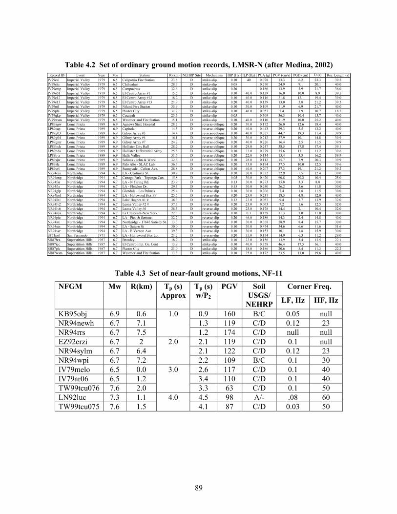
89

Table 4.2 Set of ordinary ground motion records, LMSR-N (after Medina, 2002) Record ID Event Year Mw Station R (km) NEHRP Site Mechanism fHP (Hz) fLP (Hz) PGA (g) PGV (cm/s) PGD (cm) D (s) Rec. Length (s)

IV79cal Imperial Valley 1979 6.5 Calipatria Fire Station 23.8 D strike-slip 0.10 40 0.078 13.3 6.2 23.3 39.5IV79chi Imperial Valley 1979 6.5 Chihuahua 28.7 D strike-slip 0.05 0.270 24.9 9.1 20.1 40.0IV79cmp Imperial Valley 1979 6.5 Compuertas 32.6 D strike-slip 0.20 0.186 13.9 2.9 21.7 36.0IV79e01 Imperial Valley 1979 6.5 El Centro Array #1 15.5 D strike-slip 0.10 40.0 0.139 16.0 10.0 8.9 39.5IV79e12 Imperial Valley 1979 6.5 El Centro Array #12 18.2 D strike-slip 0.10 40.0 0.116 21.8 12.1 19.4 39.0IV79e13 Imperial Valley 1979 6.5 El Centro Array #13 21.9 D strike-slip 0.20 40.0 0.139 13.0 5.8 21.2 39.5IV79nil Imperial Valley 1979 6.5 Niland Fire Station 35.9 D strike-slip 0.10 30.0 0.109 11.9 6.9 21.7 40.0IV79pls Imperial Valley 1979 6.5 Plaster City 31.7 D strike-slip 0.10 40.0 0.057 5.4 1.9 10.7 18.7IV79qkp Imperial Valley 1979 6.5 Cucapah 23.6 D strike-slip 0.05 0.309 36.3 10.4 15.7 40.0IV79wsm Imperial Valley 1979 6.5 Westmorland Fire Station 15.1 D strike-slip 0.10 40.0 0.110 21.9 10.0 25.2 40.0LP89agw Loma Prieta 1989 6.9 Agnews State Hospital 28.2 D reverse-oblique 0.20 30.0 0.172 26.0 12.6 18.4 40.0LP89cap Loma Prieta 1989 6.9 Capitola 14.5 D reverse-oblique 0.20 40.0 0.443 29.3 5.5 13.2 40.0LP89g03 Loma Prieta 1989 6.9 Gilroy Array #3 14.4 D reverse-oblique 0.10 40.0 0.367 44.7 19.3 11.4 39.9LP89g04 Loma Prieta 1989 6.9 Gilroy Array #4 16.1 D reverse-oblique 0.20 30.0 0.212 37.9 10.1 14.8 39.9LP89gmr Loma Prieta 1989 6.9 Gilroy Array #7 24.2 D reverse-oblique 0.20 40.0 0.226 16.4 2.5 11.5 39.9LP89hch Loma Prieta 1989 6.9 Hollister City Hall 28.2 D reverse-oblique 0.10 29.0 0.247 38.5 17.8 17.4 39.1LP89hda Loma Prieta 1989 6.9 Hollister Differential Array 25.8 D reverse-oblique 0.10 33.0 0.279 35.6 13.1 13.2 39.6LP89hvr Loma Prieta 1989 6.9 Halls Valley 31.6 D reverse-oblique 0.20 22.0 0.134 15.4 3.3 16.2 39.9LP89sjw Loma Prieta 1989 6.9 Salinas - John & Work 32.6 D reverse-oblique 0.10 28.0 0.112 15.7 7.9 20.3 39.9LP89slc Loma Prieta 1989 6.9 Palo Alto - SLAC Lab. 36.3 D reverse-oblique 0.20 33.0 0.194 37.5 10.0 12.5 39.6LP89svl Loma Prieta 1989 6.9 Sunnyvale - Colton Ave. 28.8 D reverse-oblique 0.10 40.0 0.207 37.3 19.1 21.2 39.2NR94cen Northridge 1994 6.7 LA - Centinela St. 30.9 D reverse-slip 0.20 30.0 0.322 22.9 5.5 12.4 30.0NR94cnp Northridge 1994 6.7 Canoga Park - Topanga Can. 15.8 D reverse-slip 0.05 30.0 0.420 60.8 20.2 10.4 25.0NR94far Northridge 1994 6.7 LA - N Faring Rd. 23.9 D reverse-slip 0.13 30.0 0.273 15.8 3.3 8.8 30.0NR94fle Northridge 1994 6.7 LA - Fletcher Dr. 29.5 D reverse-slip 0.15 30.0 0.240 26.2 3.6 11.8 30.0NR94glp Northridge 1994 6.7 Glendale - Las Palmas 25.4 D reverse-slip 0.10 30.0 0.206 7.4 1.8 11.5 30.0NR94hol Northridge 1994 6.7 LA - Holywood Stor FF 25.5 D reverse-slip 0.20 23.0 0.231 18.3 4.8 12.0 40.0NR94lh1 Northridge 1994 6.7 Lake Hughes #1 # 36.3 D reverse-slip 0.12 23.0 0.087 9.4 3.7 13.9 32.0NR94lv2 Northridge 1994 6.7 Leona Valley #2 # 37.7 D reverse-slip 0.20 23.0 0.063 7.2 1.6 12.5 32.0NR94lv6 Northridge 1994 6.7 Leona Valley #6 38.5 D reverse-slip 0.20 23.0 0.178 14.4 2.1 10.4 32.0NR94nya Northridge 1994 6.7 La Crescenta-New York 22.3 D reverse-slip 0.10 0.3 0.159 11.3 3.0 11.0 30.0NR94pic Northridge 1994 6.7 LA - Pico & Sentous 32.7 D reverse-slip 0.20 46.0 0.186 14.3 2.4 14.8 40.0NR94stc Northridge 1994 6.7 Northridge - 17645 Saticoy St. 13.3 D reverse-slip 0.10 30.0 0.368 28.9 8.4 15.7 30.0NR94stn Northridge 1994 6.7 LA - Saturn St 30.0 D reverse-slip 0.10 30.0 0.474 34.6 6.6 11.6 31.6NR94ver Northridge 1994 6.7 LA - E Vernon Ave 39.3 D reverse-slip 0.10 30.0 0.153 10.1 1.8 15.9 30.0SF71pel San Fernando 1971 6.6 LA - Hollywood Stor Lot 21.2 D reverse-slip 0.20 35.0 0.174 14.9 6.3 11.2 28.0SH87bra Superstition Hills 1987 6.7 Brawley 18.2 D strike-slip 0.10 23.0 0.156 13.9 5.4 13.5 22.1SH87icc Superstition Hills 1987 6.7 El Centro Imp. Co. Cent 13.9 D strike-slip 0.10 40.0 0.358 46.4 17.5 16.1 40.0SH87pls Superstition Hills 1987 6.7 Plaster City 21.0 D strike-slip 0.20 18.0 0.186 20.6 5.4 11.3 22.2SH87wsm Superstition Hills 1987 6.7 Westmorland Fire Station 13.3 D strike-slip 0.10 35.0 0.172 23.5 13.0 19.6 40.0

Table 4.3 Set of near-fault ground motions, NF-11

Corner Freq. NFGM Mw R(km) Tp (s) Approx

Tp (s) w/P2

PGV Soil USGS/

NEHRP LF, Hz HF, Hz

KB95obj 6.9 0.6 0.9 160 B/C 0.05 null NR94newh 6.7 7.1 1.3 119 C/D 0.12 23 NR94rrs 6.7 7.5

1.0

1.2 174 C/D null null EZ92erzi 6.7 2 2.1 119 C/D 0.1 null NR94sylm 6.7 6.4 2.1 122 C/D 0.12 23 NR94wpi 6.7 7.2

2.0

2.2 109 B/C 0.1 30 IV79melo 6.5 0.0 2.6 117 C/D 0.1 40 IV79ar06 6.5 1.2 3.4 110 C/D 0.1 40 TW99tcu076 7.6 2.0

3.0

3.3 63 C/D 0.1 50 LN92luc 7.3 1.1 4.5 98 A/- .08 60 TW99tcu075 7.6 1.5

4.0 4.1 87 C/D 0.03 50

90

Table 4.4 Set of long-duration records, LD-13

Long Duration Record Mw PGA gals

Accele- rogram

Duration

Bracketed Duration

(sec)

West. WA, Olympia 1949 6.5 71.4 80.0 41.3 Kern, Taft 021, 1952 7.7 153.0 54.2 30.3 Kern, Hol 090, 1952 7.7 43.0 78.5 31.3 Cerro Prieto, IV79, cp237 6.5 152.1 63.7 36.2 Llolleo, Chile 1985 8.0 551.9 100 36.2 Viña del Mar, Chile 1985 8.0 223.0 100 49.9 CHY015E, Taiwan 1999 7.6 142.4 150 37.5 CHY025W, Taiwan 1999 7.6 156.2 90.0 33.7 CHY046W, Taiwan 1999 7.6 139.6 90.0 33.0 CHY087W, Taiwan 1999 7.6 133.2 90.0 31.9 TCU120W, Taiwan 1999 7.6 220.8 90.0 32.6 TCU123W, Taiwan 1999 7.6 160.7 90.0 35.4 TCU138E, Taiwan 1999 7.6 191.1 150 34.1

91

Fig. 4.1 Backbone curves for hysteretic models with and without P-∆

ELASTIC STRENGTH DEMAND SPECTRALMSR-N, ξ = 0.05, Scaled at T=0.9 sec

0

1

2

3

4

5

6

0 1 2 3 4 5

Period, T (sec)

S a(T

) / S

a(T

=0.9

s)

Median84thIndividual Spectra

STANDARD DEVIATION OF LN Sa(Ti)/Sa(T=0.9)ξ = 0.05, Set of Ordinary Ground Motions LMSR-N

0

0.2

0.4

0.6

0.8

1

0 1 2 3 4 5

Period, T (sec)

St. D

ev. o

f ln

of S

a(T

)/Sa(

T=0

.9)

(a) Elastic Strength Demand Spectra (b) Dispersion of Spectra

Fig. 4.2 Spectra of ordinary GMs scaled to the same Sa at T = 0.9 s

92

EFFECT OF CYCLIC DET. ON (Sa/g)/η vs δmax/δy

Peak Oriented Model, LMSR-N, ξ=5%, P-∆=0, T=0.9 sec. αs=0.03, αc= -0.10, δc/δy=4, γs,c,k,a=Var, λ=0

0

2

4

6

8

10

0 2 4 6 8 10Inelastic / Yield Displacement, δmax / δy

(Sa/g

) / η

Non-deteriorating γs,c,k,a=Infγs,c,a=100, γk=200γs,c,a=50, γk=100γs,c,a=25, γk=50

Equal Displacement Rule

EFFECT OF CYCLIC DET. ON (Sa/g)/η vs δmax/Sd


0

2

4

6

8

10

0 0.5 1 1.5 2Inelastic / Yield Displacement, δmax / Sd

(Sa/g

) / η


(a) (Sa/g)/η - Median δmax/δy Curves (b) (Sa/g)/η - Median δmax/Sd Curves

EFFECT OF CYCLIC DET. ON δmax/δy RATIOS


0

2

4

6

8

10

0 0.5 1 1.5 2Deteriorating / NonDeteriorating Response

(Sa/g

) / η


(c) (Sa/g)/η - Median EDP ratios

Fig. 4.3 Effect of CD on EDPs, T = 0.9 s, αc = -0.1, δc/δy = 4, P-∆= 0



0

2

4

6

8

10


(Sa/g

) / η


EFFECT OF CYCLIC DET. ON δmax/δy RATIOSPeak Oriented Model, LMSR-N, ξ=5%, P-∆=0, T=0.2 sec.

αs=0.03, αc= -0.10, δc/δy=4, γs,c,k,a=Var, λ=0

0

2

4

6

8

10


(Sa/g

) / η


(a) (Sa/g)/η - Median δmax/δy Curves (b) (Sa/g)/η - Median EDP ratios

Fig. 4.4 Effect of CD on δmax/δy, T = 0.2 s, αc = -0.1, δc/δy = 4, P-∆= 0

93



0

2

4

6

8

10


(Sa/g

) / η


EFFECT OF CYCLIC DET. ON δmax/δy RATIOSPeak Oriented Model, LMSR-N, ξ=5%, P-∆=0, T=3.6 sec.

αs=0.03, αc= -0.10, δc/δy=4, γs,c,k,a=Var, λ=0

0

2

4

6

8

10


(Sa/g

) / η



Fig. 4.5 Effect of CD on δmax/δy, T = 3.6 s, αc = -0.1, δc/δy = 4, P-∆= 0

EFFECT OF αc ON (Sa/g)/η vs δmax/δy

Peak Oriented Model, LMSR-N, ξ=5%, P-∆=0, T=0.9 sec. αs=0.03, αc= Var, δc/δy=4, γs,c,k,a=Inf, λ=0

0

2

4

6

8

10


(Sa/g

) / η

Non-deteriorating αc = -0.10αc = -0.30αc = -0.50

EFFECT OF αc ON δmax/δy RATIOSPeak Oriented Model, LMSR-N, ξ=5%, P-∆=0, T=0.9 sec.

αs=0.03, αc= Var, δc/δy=4, γs,c,k,a=Inf, λ=0

0

2

4

6

8

10


(Sa/g

) / η



Fig. 4.6 Effect of αc on δmax/δy, T = 0.9 s, δc/δy = 4, γ = inf., P-∆= 0



0

2

4

6

8

10


(Sa/g

) / η


I



0

5

10

15


(Sa/g

) / η


(a) T = 0.2 s. (b) T = 3.6 s.

Fig. 4.7 Effect of αc on median δmax/δy, T = 0.2 and 3.6 s, δc/δy = 4, γ = inf., P-∆= 0

94

EFFECT OF δc/δy ON (Sa/g)/η vs δmax/δy

Peak Oriented Model, LMSR-N, ξ=5%, P-∆=0, T=0.9 sec. αs=0.03, αc= -0.10, δc/δy=Var, γs,c,k,a=Inf, λ=0

0

2

4

6

8

10

0 2 4 6 8 10 12Inelastic / Yield Displacement, δmax / δy

(Sa/g

) / η

Non-deteriorating δc/δy = 6δc/δy = 4δc/δy = 2

EFFECT OF δc/δy ON δmax/δy RATIOSPeak Oriented Model, LMSR-N, ξ=5%, P-∆=0, T=0.9 sec.

αs=0.03, αc= -0.10, δc/δy=Var, γs,c,k,a=Inf, λ=0

0

2

4

6

8

10


(Sa/g

) / η



Fig. 4.8 Effect of δc/δy on EDPs, T = 0.9 s, αc = -0.1, γ = inf., P-∆= 0



0

2

4

6

8

10

0 2 4 6 8Inelastic / Yield Displacement, δmax / δy

(Sa/g

) / η




0

5

10

15

0 2 4 6 8 10 12Inelastic / Yield Displacement, δmax / δy

(Sa/g

) / η


(a) T = 0.2 sec (b) T = 3.6 sec

Fig. 4.9 Effect of δc/δy on EDP ratios, T = 0.2 and 3.6 s, αc = -0.1, γ = inf., P-∆= 0

COLLAPSE CAPACITY Peak Oriented Model, LMSR, ξ=5%, P-∆=Var

αs=0.03, αc=Var, δc/δy=Var, γs,c,k,a=Var, λ=0

0

5

10

15

20


(Sa,

c/g) /

η

Fig. 4.10 Set of median collapse capacity spectra for peak-oriented models

95

MEDIAN (Sa/g)/η AT COLLAPSE, VARIOUS SYSTEMSPeak Oriented Model, LMSR-N, ξ=5%, P-∆=Var


0

5

10

15

20


(Sa,

c/g) /

ηγ=Inf, δc/δy=6, αc=-0.1, P-∆=0γ=100, δc/δy=4, αc=-0.1, P-∆=0γ=100, δc/δy=4, αc=-0.1, P-∆=0.1Nγ=25, δc/δy=2, αc=-0.5, P-∆=0.1N

MEDIAN (Sa/g) / η AT COLLAPSE, VARIOUS SYSTEMSPeak Oriented Model, LMSR-N, ξ=5%, P-∆=Var


0

0.2

0.4

0.6

0.8

1

1.2


Var

iatio

n / B

ase

Cas

e

γ=Inf, δc/δy=6, αc=-0.1, P-∆=0γ=100, δc/δy=4, αc=-0.1, P-∆=0γ=100, δc/δy=4, αc=-0.1, P-∆=0.1Nγ=25, δc/δy=2, αc=-0.5, P-∆=0.1N

(a) Median Collapse Capacity Spectra (b) Median Collapse Capacity Ratios

Fig. 4.11 Collapse capacity spectra for selected peak-oriented models

(Sa/g)/η at COLLAPSE vs αcPeak Oriented Model, LMSR-N, ξ=5%, P-∆=0, αs=0.03, αc=Var, δc/δy=4, γs,c,a=100, γk=200, λ=0

0

2

4

6

8

10

12

0 0.05 0.1 0.15 0.2 0.25 0.3−αc

(Sa,

c/g)/ η

T=0.1T=0.2T=0.3T=0.4T=0.5T=0.6T=0.7T=0.8T=0.9T=1.0

Fig. 4.12 Dependence of median (Sa,c/g)/η on αc; δc/δy = 4, slow CD, T = 0.1 s–1.0 s

96

EFFECT OF CAP SLOPE ON (Sa/g)/η AT COLLAPSEPeak Oriented Model, LMSR-N, ξ=5%, P-∆=0,

αs=0.03, αc=Var, δc/δy=4, γs,c,k,a=Inf

0

5

10

15

20


(Sa,

c/g) /

η

αc = -0.10 αc = -0.30 αc = -0.50



0

0.2

0.4

0.6

0.8

1

1.2


Var

iatio

n / B

ase C

ase

αc = -0.10 αc = -0.30 αc = -0.50


Fig. 4.13 Effect of αc on (Sa,c/g)/η ; δc/δy = 4, no CD, no P-∆



0

2

4

6

8

10


(Sa,

c/g) /

η

αc = -0.10 αc = -0.30 αc = -0.50

EFFECT OF CAP SLOPE ON (Sa/g) / η AT COLLAPSEPeak Oriented Model, LMSR-N, ξ=5%, P-∆=0,


0

0.2

0.4

0.6

0.8

1

1.2


Var

iatio

n / B

ase C

ase

αc = -0.10 αc = -0.30 αc = -0.50


Fig. 4.14 Effect of αc on (Sa,c/g)/η ; δc/δy = 2, no CD, no P-∆

EFFECT OF POST-CAPPING STIFFNESS ON (Sa,c/g)/η Peak Oriented Model, LMSR-N, ξ=5%, P-∆='0.1N',


0

2

4

6

8

10


(Sa,

c/g) /

η

αc = -0.10 αc = -0.30 αc = -0.50

EFFECT OF POST-CAPPING STIFFNESS ON (Sa,c/g)/ηPeak Oriented Model, LMSR-N, ξ=5%, P-∆='0.1N',


0

0.2

0.4

0.6

0.8

1

1.2


Var

iatio

n / B

ase C

ase

αc = -0.10 αc = -0.30 αc = -0.50


Fig. 4.15 Effect of αc on (Sa,c/g)/η ; δc/δy = 4, no CD, small P-∆

97



0

2

4

6

8

10


(Sa,

c/g) /

η

αc = -0.10 αc = -0.30 αc = -0.50



0

0.2

0.4

0.6

0.8

1

1.2


Var

iatio

n / B

ase C

ase

αc = -0.10 αc = -0.30 αc = -0.50


Fig. 4.16 Effect of αc on (Sa,c/g)/η ; δc/δy = 2, no CD, small P-∆


αs=0.03, αc=Var, δc/δy=4, γs,c,k,a=50

0

5

10

15

20


(Sa,

c/g) /

η

αc = -0.10 αc = -0.30 αc = -0.50


αs=0.03, αc=Var, δc/δy=4, γs,c,k,a=50

0

0.2

0.4

0.6

0.8

1

1.2


Var

iatio

n / B

ase C

ase

αc = -0.10 αc = -0.30 αc = -0.50


Fig. 4.17 Effect of αc on (Sa,c/g)/η ; δc/δy = 4, medium CD, no P-∆

EFFECT OF CAP SLOPE ON (Sa/g)/η AT COLLAPSEBilinear Model, LMSR-N, ξ=5%, P-∆=0,


0

5

10

15

20


(Sa,

c/g) /

η

αc = -0.10 αc = -0.30 αc = -0.50

EFFECT OF CAP SLOPE ON (Sa/g)/η AT COLLAPSEBilinear Model, LMSR-N, ξ=5%, P-∆=0,


0

0.2

0.4

0.6

0.8

1

1.2


Var

iatio

n / B

ase C

ase

αc = -0.10 αc = -0.30 αc = -0.50


Fig. 4.18 Effect of αc on (Sa,c/g)/η ; bilinear model, δc/δy = 4, no CD, no P-∆

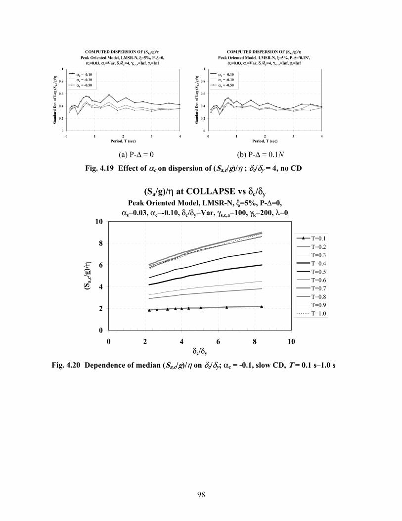
98

COMPUTED DISPERSION OF (Sa,c/g)/ηPeak Oriented Model, LMSR-N, ξ=5%, P-∆=0,

αs=0.03, αc=Var, δc/δy=4, γs,c,a=Inf, γk=Inf

0

0.2

0.4

0.6

0.8

1

0 1 2 3 4Period, T (sec)

Stan

dard

Dev

of L

og (S

a,c/g

)/ η

αc = -0.10 αc = -0.30 αc = -0.50

COMPUTED DISPERSION OF (Sa,c/g)/ηPeak Oriented Model, LMSR-N, ξ=5%, P-∆='0.1N',

αs=0.03, αc=Var, δc/δy=4, γs,c,a=Inf, γk=Inf

0

0.2

0.4

0.6

0.8

1


Stan

dard

Dev

of L

og (S

a,c/g

)/ η

αc = -0.10 αc = -0.30 αc = -0.50

(a) P-∆ = 0 (b) P-∆ = 0.1N

Fig. 4.19 Effect of αc on dispersion of (Sa,c/g)/η ; δc/δy = 4, no CD

(Sa/g)/η at COLLAPSE vs δc/δyPeak Oriented Model, LMSR-N, ξ=5%, P-∆=0,

αs=0.03, αc=-0.10, δc/δy=Var, γs,c,a=100, γk=200, λ=0

0

2

4

6

8

10

0 2 4 6 8 10δc/δy

(Sa,

c/g)/ η

T=0.1T=0.2T=0.3T=0.4T=0.5T=0.6T=0.7T=0.8T=0.9T=1.0

Fig. 4.20 Dependence of median (Sa,c/g)/η on δc/δy; αc = -0.1, slow CD, T = 0.1 s–1.0 s

99

EFFECT OF δc / δy ON MEDIAN (Sa/g)/η AT COLLAPSEPeak Oriented Model, LMSR-N, ξ=5%, P-∆=0

αs=0.03, αc=-0.10, δc/δy=Var, γs,c,k,a=Inf

0

5

10

15

20


(Sa,

c/g) /

η

δc / δy = 6δc / δy = 4δc / δy = 2

EFFECT OF δc / δy ON MEDIAN (Sa/g) / η AT COLLAPSEPeak Oriented Model, LMSR-N, ξ=5%, P-∆=0


0

0.2

0.4

0.6

0.8

1

1.2


Var

iatio

n / B

ase C

ase

δc / δy = 6δc / δy = 4δc / δy = 2


Fig. 4.21 Effect of δc/δy on (Sa,c/g)/η ; αc = -0.1, no CD, no P-∆



0

2

4

6

8

10


(Sa,

c/g) /

η

δc / δy = 6δc / δy = 4δc / δy = 2



0

0.2

0.4

0.6

0.8

1

1.2


Var

iatio

n / B

ase C

ase

δc / δy = 6δc / δy = 4δc / δy = 2


Fig. 4.22 Effect of δc/δy on (Sa,c/g)/η ; αc = -0.3, no CD, no P-∆

EFFECT OF δc / δy ON MEDIAN (Sa/g)/η AT COLLAPSEPeak Oriented Model, LMSR-N, ξ=5%, P-∆='0.1N',


0

2

4

6

8

10


(Sa,

c/g) /

η

δc / δy = 6δc / δy = 4δc / δy = 2

EFFECT OF δc / δy ON MEDIAN (Sa/g) / η AT COLLAPSEPeak Oriented Model, LMSR-N, ξ=5%, P-∆='0.1N',


0

0.2

0.4

0.6

0.8

1

1.2


Var

iatio

n / B

ase

Cas

e

δc / δy = 6δc / δy = 4δc / δy = 2


Fig. 4.23 Effect of δc/δy on (Sa,c/g)/η ; αc = -0.1, no CD, small P-∆

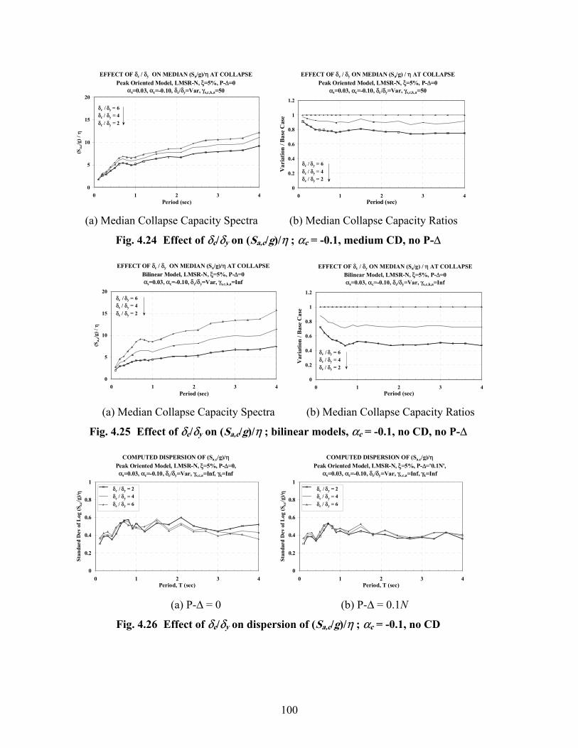
100


αs=0.03, αc=-0.10, δc/δy=Var, γs,c,k,a=50

0

5

10

15

20


(Sa,

c/g) /

η

δc / δy = 6δc / δy = 4δc / δy = 2


αs=0.03, αc=-0.10, δc/δy=Var, γs,c,k,a=50

0

0.2

0.4

0.6

0.8

1

1.2


Var

iatio

n / B

ase C

ase

δc / δy = 6δc / δy = 4δc / δy = 2


Fig. 4.24 Effect of δc/δy on (Sa,c/g)/η ; αc = -0.1, medium CD, no P-∆

EFFECT OF δc / δy ON MEDIAN (Sa/g)/η AT COLLAPSEBilinear Model, LMSR-N, ξ=5%, P-∆=0αs=0.03, αc=-0.10, δc/δy=Var, γs,c,k,a=Inf

0

5

10

15

20


(Sa,

c/g) /

η

δc / δy = 6δc / δy = 4δc / δy = 2

EFFECT OF δc / δy ON MEDIAN (Sa/g) / η AT COLLAPSEBilinear Model, LMSR-N, ξ=5%, P-∆=0αs=0.03, αc=-0.10, δc/δy=Var, γs,c,k,a=Inf

0

0.2

0.4

0.6

0.8

1

1.2


Var

iatio

n / B

ase

Cas

e

δc / δy = 6δc / δy = 4δc / δy = 2


Fig. 4.25 Effect of δc/δy on (Sa,c/g)/η ; bilinear models, αc = -0.1, no CD, no P-∆

COMPUTED DISPERSION OF (Sa,c/g)/ηPeak Oriented Model, LMSR-N, ξ=5%, P-∆=0, αs=0.03, αc=-0.10, δc/δy=Var, γs,c,a=Inf, γk=Inf

0

0.2

0.4

0.6

0.8

1


Stan

dard

Dev

of L

og (S

a,c/g

)/ η

δc / δy = 2δc / δy = 4δc / δy = 6


αs=0.03, αc=-0.10, δc/δy=Var, γs,c,a=Inf, γk=Inf

0

0.2

0.4

0.6

0.8

1


Stan

dard

Dev

of L

og (S

a,c/g

)/ η

δc / δy = 2δc / δy = 4δc / δy = 6

(a) P-∆ = 0 (b) P-∆ = 0.1N

Fig. 4.26 Effect of δc/δy on dispersion of (Sa,c/g)/η ; αc = -0.1, no CD

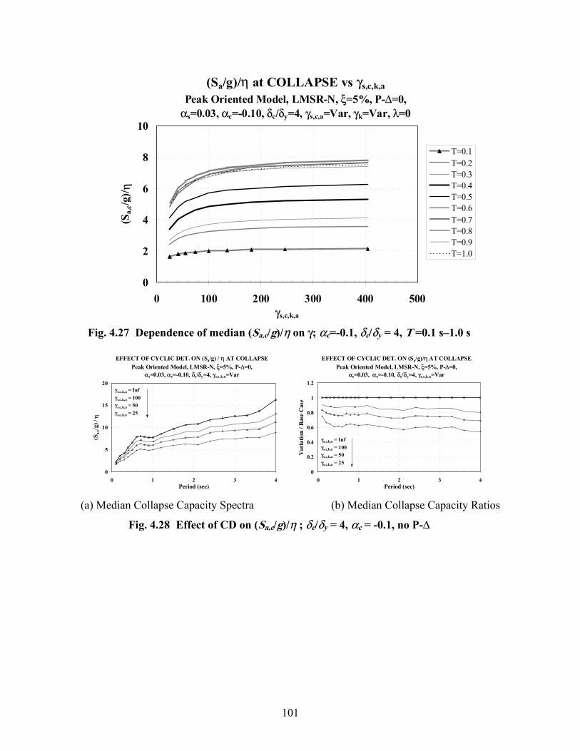
101

(Sa/g)/η at COLLAPSE vs γs,c,k,aPeak Oriented Model, LMSR-N, ξ=5%, P-∆=0,

αs=0.03, αc=-0.10, δc/δy=4, γs,c,a=Var, γk=Var, λ=0

0

2

4

6

8

10

0 100 200 300 400 500γs,c,k,a

(Sa,

c/g)/ η

T=0.1T=0.2T=0.3T=0.4T=0.5T=0.6T=0.7T=0.8T=0.9T=1.0

Fig. 4.27 Dependence of median (Sa,c/g)/η on γ; αc=-0.1, δc/δy = 4, T =0.1 s–1.0 s

EFFECT OF CYCLIC DET. ON (Sa/g) / η AT COLLAPSE

Peak Oriented Model, LMSR-N, ξ=5%, P-∆=0, αs=0.03, αc=-0.10, δc/δy=4, γs,c,k,a=Var

0

5

10

15

20


(Sa,

c/g) /

η

γs,c,k,a = Infγs,c,k,a = 100γs,c,k,a = 50γs,c,k,a = 25

EFFECT OF CYCLIC DET. ON (Sa/g)/η AT COLLAPSEPeak Oriented Model, LMSR-N, ξ=5%, P-∆=0,

αs=0.03, αc=-0.10, δc/δy=4, γs,c,k,a=Var

0

0.2

0.4

0.6

0.8

1

1.2


Var

iatio

n / B

ase

Cas

e



Fig. 4.28 Effect of CD on (Sa,c/g)/η ; δc/δy = 4, αc = -0.1, no P-∆

102

NHE at (Sa/g)/η AT COLLAPSEPeak Oriented Model, LMSR-N, ξ=5%, P-∆=0,


0

10

20

30

40

50

60


NH

E at

(Sa,

c/g)/ η


NHE at (Sa/g)/η AT COLLAPSEPeak Oriented Model, LMSR-N, ξ=5%, P-∆=0,


0

0.2

0.4

0.6

0.8

1

1.2


Var

iatio

n / B

ase

Cas

e


(a) Median NHE at (Sa,c/g)/η (b) Ratios of Median NHE at (Sa,c/g)/η

Fig. 4.29 NHE associated with (Sa,c/g)/η for different CD rates; δc/δy = 4, αc = -0.1, no P-∆



0

2

4

6

8

10


(Sa,

c/g) /

η


EFFECT OF CYCLIC DET. ON (Sa/g) / η AT COLLAPSEPeak Oriented Model, LMSR-N, ξ=5%, P-∆=0,


0

0.2

0.4

0.6

0.8

1

1.2


Var

iatio

n / B

ase

Cas

e



Fig. 4.30 Effect of CD on (Sa,c/g)/η ; δc/δy = 2, αc = -0.1, no P-∆

EFFECT OF CYCLIC DET. ON (Sa/g) / η AT COLLAPSEPeak Oriented Model, LMSR-N, ξ=5%, P-∆=0,


0

2

4

6

8

10


(Sa,

c/g) /

η




0

0.2

0.4

0.6

0.8

1

1.2


Var

iatio

n / B

ase

Cas

e



Fig. 4.31 Effect of CD on (Sa,c/g)/η ; δc/δy = 4, αc = -0.3 no P-∆

103

EFFECT OF CYCLIC DET. ON (Sa/g) / η AT COLLAPSEPeak Oriented Model, LMSR-N, ξ=5%, P-∆='0.1N',


0

2

4

6

8

10


(Sa,

c/g) /

η


EFFECT OF CYCLIC DET. ON (Sa/g)/η AT COLLAPSEPeak Oriented Model, LMSR-N, ξ=5%, P-∆='0.1N',


0

0.2

0.4

0.6

0.8

1

1.2


Var

iatio

n / B

ase

Cas

e



Fig. 4.32 Effect of CD on (Sa,c/g)/η ; δc/δy = 4, αc = -0.1, small P-∆

EFFECT OF CYCLIC DET. ON (Sa/g)/η AT COLLAPSEBilinear Model, LMSR-N, ξ=5%, P-∆=0,


0

5

10

15

20


(Sa,

c/g) /

η


EFFECT OF CYCLIC DET. ON (Sa/g)/η AT COLLAPSEBilinear Model, LMSR-N, ξ=5%, P-∆=0,


0

0.2

0.4

0.6

0.8

1

1.2


Var

iatio

n / B

ase

Cas

e



Fig. 4.33 Effect of CD on (Sa,c/g)/η ; bilinear models, δc/δy = 4, αc = -0.1, no P-∆

COMPUTED DISPERSION OF (Sa,c/g)/ηPeak Oriented Model, LMSR-N, ξ=5%, P-∆=0,

αs=0.03, αc=-0.10, δc/δy=4, γs,c,a=Var, γk=Var

0

0.2

0.4

0.6

0.8

1


Stan

dard

Dev

of L

og (S

a,c/g

)/ η



αs=0.03, αc=-0.10, δc/δy=4, γs,c,a=Var, γk=Var

0

0.2

0.4

0.6

0.8

1


Stan

dard

Dev

of L

og (S

a,c/g

)/ η


(a) P-∆ = 0 (b) P-∆ = 0.1N

Fig. 4.34 Effect of CD on dispersion of (Sa,c/g)/η ; αc = -0.1, δc/δy = 4

104

STABILITY COEFFICIENT FOR SDOF SYSTEMS

0%

2%

4%

6%

8%

10%

12%

14%

16%

0 1 2 3 4Period of SDOF System (sec)

Stab

ility

Coe

ffic

ient

Small P-∆Large P-∆

Fig. 4.35 Stability coefficients for SDOF parameter study

EFFECT OF P-∆ ON (Sa/g)/η AT COLLAPSEPeak Oriented Model, LMSR-N, ξ=5%, P-∆=Var,

αs=0.03, αc=-0.10, δc/δy=4, γs,c,a=Inf, γk=Inf

0

5

10

15

20


(Sa,

c/g) /

η

P - ∆ = 0P - ∆ = '0.1 N'P - ∆ = '0.2 N'

EFFECT OF P-∆ ON (Sa/g)/η AT COLLAPSEPeak Oriented Model, LMSR-N, ξ=5%, P-∆=Var


0

0.2

0.4

0.6

0.8

1

1.2


Var

iatio

n / B

ase C

ase

P - ∆ = 0P - ∆ = '0.1 N'P - ∆ = '0.2 N'


Fig. 4.36 Effect of P-∆ on (Sa,c/g)/η ; δc/δy = 4, αc = -0.1, no CD


αs=0.03, αc=-0.10, δc/δy=2, γs,c,k,a=Inf

0

2

4

6

8

10


(Sa,

c/g) /

η

P - ∆ = 0P - ∆ = '0.1 N'P - ∆ = '0.2 N'



0

0.2

0.4

0.6

0.8

1

1.2


Var

iatio

n / B

ase C

ase

P - ∆ = 0P - ∆ = '0.1 N'P - ∆ = '0.2 N'



105



0

2

4

6

8

10


(Sa,

c/g) /

η

P - ∆ = 0P - ∆ = '0.1 N'P - ∆ = '0.2 N'



0

0.2

0.4

0.6

0.8

1

1.2


Var

iatio

n / B

ase C

ase

P - ∆ = 0P - ∆ = '0.1 N'P - ∆ = '0.2 N'




αs=0.03, αc=-0.10, δc/δy=4, γs,c,a=50, γk=100

0

5

10

15

20


(Sa,

c/g) /

η

P - ∆ = 0P - ∆ = '0.1 N'P - ∆ = '0.2 N'


αs=0.03, αc=-0.10, δc/δy=4, γs,c,a=50, γk=100

0

0.2

0.4

0.6

0.8

1

1.2


Var

iatio

n / B

ase C

ase

P - ∆ = 0P - ∆ = '0.1 N'P - ∆ = '0.2 N'


Fig. 4.39 Effect of P-∆ on (Sa,c/g)/η ; δc/δy = 4, αc = -0.1, medium CD

EFFECT OF P-∆ ON (Sa/g)/η AT COLLAPSEBilinear Model, LMSR-N, ξ=5%, P-∆=0,


0

5

10

15

20


(Sa,

c/g) /

η

P - ∆ = 0P - ∆ = '0.1 N'P - ∆ = '0.2 N'

EFFECT OF P-∆ ON (Sa/g)/η AT COLLAPSEBilinear Model, LMSR-N, ξ=5%, P-∆=Var,


0

0.2

0.4

0.6

0.8

1

1.2


Var

iatio

n / B

ase

Cas

e

P - ∆ = 0P - ∆ = '0.1 N'P - ∆ = '0.2 N'


Fig. 4.40 Effect of P-∆ effect on (Sa,c/g)/η ; bilinear models, δc/δy = 4, αc = -0.1, no CD

106

COLLAPSE CAPACITYPinching / Peak Oriented Model, LMSR-N, ξ=5%, P-∆=0,

αs=0.03, αc=Var, δc/δy=Var, γs,c,k,a=Var, κf,d=0.25, λ=0

0

0.2

0.4

0.6

0.8

1

1.2

1.4


Var

iatio

n / B

ase C

ase

COLLAPSE CAPACITYBilinear / Peak Oriented Model, LMSR-N, ξ=5%, P-∆=0,


0

0.2

0.4

0.6

0.8

1

1.2

1.4


Var

iatio

n / B

ase

Cas

e

(a) Pinching / Peak-Oriented (b) Bilinear / Peak-Oriented

Fig. 4.41 Median collapse capacity ratios for different hysteretic models, P-∆ = 0

COLLAPSE CAPACITYPinching / Peak Oriented Model, LMSR-N, ξ=5%, P-∆='0.1N'

αs=0.03, αc=Var, δc/δy=Var, γs,c,k,a=Var, κf,d=0.25, λ=0

0

0.2

0.4

0.6

0.8

1

1.2

1.4


Var

iatio

n / B

ase C

ase

COLLAPSE CAPACITYBilinear/Peak Oriented Model, LMSR-N, ξ=5%, P-∆='0.1N'


0

0.2

0.4

0.6

0.8

1

1.2

1.4


Var

iatio

n / B

ase

Cas

e

(a) Pinching / Peak-Oriented (b) Bilinear / Peak-Oriented

Fig. 4.42 Median collapse capacity ratios for different hysteretic models, P-∆ = 0.1N COLLAPSE CAPACITY RATIOS FOR HYST. MODELSBilinear / Peak Oriented Model, LMSR-N, ξ=5%, P-∆=0,

αs=0.03, αc=Var, δc/δy=Var, γs,c,k,a=Inf

0

0.2

0.4

0.6

0.8

1

1.2


Bili

near

/ Pe

ak O

rien

ted

αs =-0.10, δc/δy = 2αs =-0.30, δc/δy = 6

Fig. 4.43 Examples of collapse capacity ratios for bilinear / peak-oriented hysteretic models

107

EFFECT OF HYST. MODEL ON (Sa/g)/η AT COLLAPSEBilinear / Peak Oriented Model, LMSR-N, ξ=5%, P-∆=0


0

0.2

0.4

0.6

0.8

1

1.2


Bilin

ear

/ Pea

k O

rien

ted

αc = -0.10 αc = -0.30 αc = -0.50

EFFECT OF HYST. MODEL ON (Sa/g)/η AT COLLAPSEBilinear / Peak Oriented Model, LMSR-N, ξ=5%, P-∆=0


0

0.2

0.4

0.6

0.8

1

1.2


Bilin

ear

/ Pea

k O

rien

ted

αc = -0.10 αc = -0.30 αc = -0.50

(a) δc/δy = 2 (b) δc/δy = 6

Fig. 4.44 Effect of hysteretic model on median collapse capacity; systems with different δc/δy and αc values

EFFECT OF HYST. MODEL ON (Sa/g) / η AT COLLAPSE

Bilinear / Peak Oriented Model, LMSR-N, ξ=5%, P-∆=0,αs=0.03, αc=-0.10, δc/δy=4, γs,c,k,a=Var

0

0.2

0.4

0.6

0.8

1

1.2


Bili

near

/ Pe

ak O

rien

ted


EFFECT OF HYST. MODEL ON (Sa/g) / η AT COLLAPSEBilinear / Peak Oriented Model, LMSR-N, ξ=5%, P-∆=0,


0

0.2

0.4

0.6

0.8

1

1.2


Bilin

ear

/ Pea

k O

rien

ted


(a) αc = -0.1, δc/δy = 4 (b) αc = -0.1, δc/δy = 2

Fig. 4.45 Effect of hysteretic model on median collapse capacity; systems with different CD rates

108

INCREMENT IN (Sa/g)/η after reaching δc

Peak Oriented Model, LMSR-N, ξ=5%, P-∆=0 αs=0.03, αc= -0.10 , δc/δy=4, γs,c,k,a=Var, λ=0

0.00

0.50

1.00

1.50

2.00

2.50


[Sa,

c/ η] /

[(S a

/η(δ

c/ δy=

4)]

γs,c,k,a=Infγs,c,a=100, γk=200γs,c,a=50, γk=100γs,c,a=25, γk=50


Peak Oriented Model, LMSR-N, ξ=5%, P-∆=0 αs=0.03, αc=Var, δc/δy=4, γs,c,k,a=Inf, λ=0

0.00

0.50

1.00

1.50

2.00

2.50


[Sa,

c/ η] /

[(S a

/η(δ

c/ δy=

4)]

αc = -0.10αc = -0.30αc = -0.50

(a) Different CD Rates (b) Different αc Slopes


Peak Oriented Model, LMSR-N, ξ=5%, P-∆=0 αs=0.03, αc= -0.10 , δc/δy=Var, γs,c,k,a=Inf, λ=0

0.00

1.00

2.00

3.00

4.00

5.00


[Sa,

c/ η] /

[(S a

/η(δ

c/ δy=

6,4,

2)]

δc/δy = 6δc/δy = 4δc/δy = 2

(c) Different δc/δy Ratios

Fig. 4.46 Median ratios of (Sa,c/g)/η over (Sa/g)/η when δ = δc; P-∆ =0

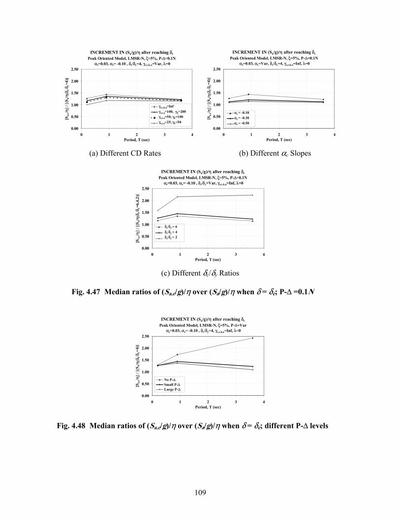
109


Peak Oriented Model, LMSR-N, ξ=5%, P-∆=0.1N αs=0.03, αc= -0.10 , δc/δy=4, γs,c,k,a=Var, λ=0

0.00

0.50

1.00

1.50

2.00

2.50


[Sa,

c/ η] /

[(S a

/η(δ

c/ δy=

4)]



Peak Oriented Model, LMSR-N, ξ=5%, P-∆=0.1N αs=0.03, αc=Var, δc/δy=4, γs,c,k,a=Inf, λ=0

0.00

0.50

1.00

1.50

2.00

2.50


[Sa,

c/ η] /

[(S a

/η(δ

c/ δy=

4)]

αc = -0.10αc = -0.30αc = -0.50

(a) Different CD Rates (b) Different αc Slopes


Peak Oriented Model, LMSR-N, ξ=5%, P-∆=0.1N αs=0.03, αc= -0.10 , δc/δy=Var, γs,c,k,a=Inf, λ=0

0.00

0.50

1.00

1.50

2.00

2.50


[Sa,

c/ η] /

[(S a

/η(δ

c/ δy=

6,4,

2)]

δc/δy = 6δc/δy = 4δc/δy = 2

(c) Different δc/δy Ratios

Fig. 4.47 Median ratios of (Sa,c/g)/η over (Sa/g)/η when δ = δc; P-∆ =0.1N


Peak Oriented Model, LMSR-N, ξ=5%, P-∆=Var αs=0.03, αc= -0.10 , δc/δy=4, γs,c,k,a=Inf, λ=0

0.00

0.50

1.00

1.50

2.00

2.50


[Sa,

c/ η] /

[(S a

/η(δ

c/ δy=

4)]

No P-∆Small P-∆Large P-∆

Fig. 4.48 Median ratios of (Sa,c/g)/η over (Sa/g)/η when δ = δc; different P-∆ levels

110

HYSTERETIC LOOPS, (Sa/g)/η=10Peak Oriented Model, NOR94hol, T=0.6 s., ξ=5%, P-∆ = 0

αs=0.05, αc= -0.10 , δc/δy=4, γs,c,k,a=Var, λ=Var

-150

-100

-50

0

50

100

150

-5 0 5 10 15 20 25Displacement, δ

Forc

e (K

f-f)

Residual = 0.4 FyResidual = 0.2 Fy

(a) P-∆ = 0

HYSTERETIC LOOPS, (Sa/g)/η=10Peak Oriented Model, NOR94hol, T=0.6 s., ξ=5%, P-∆ ='0.1N'

αs=0.05, αc= -0.10 , δc/δy=4, γs,c,k,a=Var, λ=Var

-150

-100

-50

0

50

100

150

-10 0 10 20 30 40Displacement, δ (cm)

Forc

e (K

g-f)

Residual = 0.4 FyResidual = 0.2 Fy

(b) P-∆ = 0.1N

Fig. 4.49 Hysteretic response for a system with residual strength

111

δf/δy RATIOS FOR SYSTEMS W/RESIDUAL STRENGTHP-∆='0.1N', αs=0.03, αc=-0.10, δc/δy=6

0

20

40

60


δ f /

δ y R

atio

s

No ResidualResidual = 0.2 FyResidual = 0.4 Fy

δf/δy RATIOS FOR SYSTEMS W/RESIDUAL STRENGTHP-∆='0.1N', αs=0.03, αc=-0.30, δc/δy=2

0

20

40

60


δ f /

δ y R

atio

s

No ResidualResidual = 0.2 FyResidual = 0.4 Fy

(a) Ductile Systems (b) Non-ductile Systems

Fig. 4.50 Normalized collapse displacements (δf /δy) for systems with residual strength

RESIDUAL EFFECT ON MEDIAN (Sa,c/g)/ηPeak Oriented Model, LMSR-N, ξ=5%, P-∆='0.1N',

αs=0.03, αc=-0.10, δc/δy=6, γs,c,k,a=Inf, λ=Var

0

2

4

6

8

10


(Sa,

c/g) /

η

λ = 0.4λ = 0.2λ = 0


αs=0.03, αc=-0.10, δc/δy=6, γs,c,k,a=Inf, λ=Var

0

0.5

1

1.5

2


Var

iatio

n / B

ase C

ase

λ = 0.4λ = 0.2λ = 0


Fig. 4.51 Effect of residual strength on (Sa,c/g)/η for ductile systems


αs=0.03, αc=-0.30, δc/δy=2, γs,c,k,a=Inf, κf,d=N.A., λ=Var

0

2

4

6

8

10


(Sa,

c/g) /

η

λ = 0.4 λ = 0.2 λ = 0



0

0.5

1

1.5

2


Var

iatio

n / B

ase C

ase

λ = 0.4 λ = 0.2 λ = 0


Fig. 4.52 Effect of residual strength on (Sa,c/g)/η for non-ductile systems

112

RESIDUAL EFFECT ON MEDIAN (Sa,c/g)/ηPeak Oriented Model, LMSR-N, ξ=5%, P-∆='0.1N', αs=0.03, αc=-0.10, δc/δy=6, γs,c,a=50, γk=100, λ=Var

0

2

4

6

8

10


(Sa,

c/g) /

η

λ = 0.4 λ = 0.2 λ = 0


0

0.5

1

1.5

2


Var

iatio

n / B

ase C

ase

λ = 0.4 λ = 0.2 λ = 0


Fig. 4.53 Effect of residual strength on (Sa,c/g)/η for ductile systems with CD


0

2

4

6

8

10


(Sa,

c/g) /

η

λ = 0.4λ = 0.2λ = 0


0

0.5

1

1.5

2


Var

iatio

n / B

ase C

ase

λ = 0.4λ = 0.2λ = 0


Fig. 4.54 Effect of residual strength on (Sa,c/g)/η for non-ductile systems with CD

MAX / YIELD DISP at COLLAPSE vs TPeak Oriented Model, LMSR-N, ξ=5%, P-∆=0.1N,

αs=0.03, αcap=-0.10, δc/δy=6, γs,c,k,a=Inf, λ=0.4

0

20

40

60

80


Max

/Yie

ld D

isp.

at C

ol, δ

max

/ δy

MAX / YIELD DISP at COLLAPSE vs TPeak Oriented Model, LMSR-N, ξ=5%, P-∆=0.1N, αs=0.03, αcap=-0.10, δc/δy=6, γs,c,k,a=50, γk=100, λ=0.4

0

20

40

60

80


Max

/Yie

ld D

isp.

at C

ol, δ

max

/ δy

(a) No CD (b) Medium CD

Fig. 4.55 δmax/δy at collapse for a ductile system

113

MAX / YIELD DISP at COLLAPSE vs TPeak Oriented Model, LMSR-N, ξ=5%, P-∆=0.1N,

αs=0.03, αcap=-0.10, δc/δy=6, γs,c,k,a=Inf, λ=0.4

0

20

40

60

80


Max

/Yie

ld D

isp.

at C

ol, δ

max

/ δy

δf (λ>0) <= 1.6 δf (λ=0)

Fig. 4.56 δmax/δy at collapse for a ductile system when δf (λ>0) ≤ 1.6 δf (λ=0)

RESIDUAL EFFECT ON MEDIAN (Sa,c/g)/η

Peak Oriented Model, LMSR-N, ξ=5%, P-∆='0.1N', αs=0.03, αc=-0.10, δc/δy=6, γs,c,k,a=Inf, λ=Var

0

0.5

1

1.5

2


Var

iatio

n / B

ase C

ase

δf (λ>0) = 1.6 δf (λ=0)

λ = 0.4 λ = 0.2 λ = 0



0

0.5

1

1.5

2


Var

iatio

n / B

ase C

ase

δf (λ>0) = 1.6 δf (λ=0)

λ = 0.4λ = 0.2λ = 0

(a) Ductile Systems (b) Non-ductile Systems

Fig. 4.57 Effect of residual strength on collapse displacements considering δf (λ>0) ≤ 1.6 δf (λ=0)

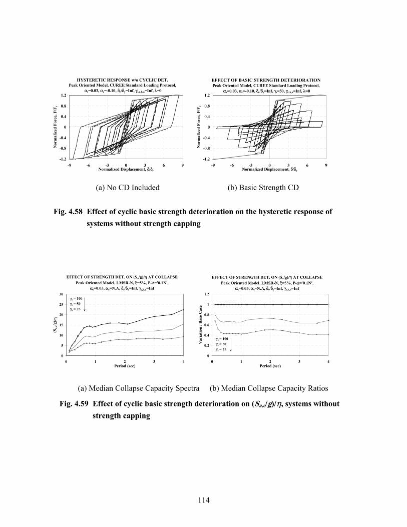
114

HYSTERETIC RESPONSE w/o CYCLIC DET.Peak Oriented Model, CUREE Standard Loading Protocol,

αs=0.03, αc=-0.10, δc/δy=Inf, γs,c,k,a=Inf, λ=0

-1.2

-0.8

-0.4

0

0.4

0.8

1.2


Nor

mal

ized

For

ce, F

/Fy

EFFECT OF BASIC STRENGTH DETERIORATIONPeak Oriented Model, CUREE Standard Loading Protocol,

αs=0.03, αc=-0.10, δc/δy=Inf, γs=50, γc,k,a=Inf, λ=0

-1.2

-0.8

-0.4

0

0.4

0.8

1.2


Nor

mal

ized

For

ce, F

/Fy

(a) No CD Included (b) Basic Strength CD

Fig. 4.58 Effect of cyclic basic strength deterioration on the hysteretic response of systems without strength capping

EFFECT OF STRENGTH DET. ON (Sa/g)/η AT COLLAPSEPeak Oriented Model, LMSR-N, ξ=5%, P-∆='0.1N',

αs=0.03, αc=N.A, δc/δy=Inf, γc,k,a=Inf

0

5

10

15

20

25

30


(Sa,

c/g)/ η

γs = 100γs = 50γs = 25

EFFECT OF STRENGTH DET. ON (Sa/g)/η AT COLLAPSEPeak Oriented Model, LMSR-N, ξ=5%, P-∆='0.1N',

αs=0.03, αc=N.A, δc/δy=Inf, γc,k,a=Inf

0

0.2

0.4

0.6

0.8

1

1.2


Var

iatio

n / B

ase

Cas

e

γs = 100γs = 50γs = 25


Fig. 4.59 Effect of cyclic basic strength deterioration on (Sa,c/g)/η, systems without strength capping

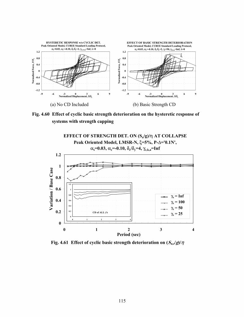
115

HYSTERETIC RESPONSE w/o CYCLIC DET.Peak Oriented Model, CUREE Standard Loading Protocol,

αs=0.03, αc=-0.10, δc/δy=2, γs,c,k,a=Inf, λ=0

-1.2

-0.8

-0.4

0

0.4

0.8

1.2


Nor

mal

ized

For

ce, F

/Fy

EFFECT OF BASIC STRENGTH DETERIORATIONPeak Oriented Model, CUREE Standard Loading Protocol,

αs=0.03, αc=-0.10, δc/δy=2, γs=50, γc,k,a=Inf, λ=0

-1.2

-0.8

-0.4

0

0.4

0.8

1.2


Nor

mal

ized

For

ce, F

/Fy

δc

(a) No CD Included (b) Basic Strength CD

Fig. 4.60 Effect of cyclic basic strength deterioration on the hysteretic response of systems with strength capping

EFFECT OF STRENGTH DET. ON (Sa/g)/η AT COLLAPSE

Peak Oriented Model, LMSR-N, ξ=5%, P-∆='0.1N', αs=0.03, αc=-0.10, δc/δy=4, γc,k,a=Inf

0

0.2

0.4

0.6

0.8

1

1.2


Var

iatio

n / B

ase

Cas

e

γs = Infγs = 100γs = 50γs = 25

0

0.2

0.4

0.6

0.8

1

1.2

0 1 2 3 4

CD of ALL γ's

Fig. 4.61 Effect of cyclic basic strength deterioration on (Sa,c/g)/η

116

EFFECT OF POST-CAPPING STRENGTH DET.Peak Oriented Model, CUREE Standard Loading Protocol,

αs=0.03, αc=-0.10, δc/δy=2, γc=50, γs,k,a=Inf, λ=0

-1.2

-0.8

-0.4

0

0.4

0.8

1.2


Nor

mal

ized

For

ce, F

/Fy

δc

HYSTERETIC RESPONSE with CYCLIC DET.Peak Oriented Model, CUREE Standard Loading Protocol,

αs=0.03, αc=-0.10, δc/δy=2, γs,c,k,a=50, λ=0

-1.2

-0.8

-0.4

0

0.4

0.8

1.2


Nor

mal

ized

For

ce, F

/Fy

(a) Post-Capping Strength CD (b) CD for all Four Modes

Fig. 4.62 Effect of cyclic post-capping strength deterioration on the hysteretic response

STRENGTH CAPPING DET. EFFECT ON (Sa/g)/η AT COL.Peak Oriented Model, LMSR-N, ξ=5%, P-∆='0.1N', αs=0.03, αc=-0.10, δc/δy=4, γs,k,a=Inf, κf,d=N.A., λ=0

0

0.2

0.4

0.6

0.8

1

1.2


Var

iatio

n / B

ase

Cas

e

γc = Infγc = 100γc = 50γc = 25

0

0.2

0.4

0.6

0.8

1

1.2

0 1 2 3 4

CD of ALL γ's

Fig. 4.63 Effect of cyclic post-capping strength deterioration on (Sa,c/g)/η

117

EFFECT OF UNLOADING STIFFNESS DET.Peak Oriented Model, CUREE Standard Loading Protocol,

αs=0.03, αc=-0.10, δc/δy=2, γk=100, γs,c,a=Inf, λ=0

-1.2

-0.8

-0.4

0

0.4

0.8

1.2


Nor

mal

ized

For

ce, F

/Fy

Fig. 4.64 Effect of cyclic unloading stiffness deterioration on the hysteretic response of a system with strength capping

UNLOADING STIFFNESS DET. EFFECT ON (Sa,c/g)/ηPeak Oriented Model, LMSR-N, ξ=5%, P-∆='0.1N', αs=0.03, αc=-0.10, δc/δy=4, γs,c,a=Inf, κf,d=N.A., λ=0

0

0.2

0.4

0.6

0.8

1

1.2


Var

iatio

n / B

ase

Cas

e

γk = Infγk = 200γk = 100γk = 50

Fig. 4.65 Effect of cyclic unloading stiffness deterioration on (Sa,c/g)/η

118

EFFECT OF ACCELERATED STIFFNESS DET.Peak Oriented Model, CUREE Standard Loading Protocol,

αs=0.03, αc=-0.10, δc/δy=2, γa=50, γs,c,k=Inf, λ=0

-1.2

-0.8

-0.4

0

0.4

0.8

1.2


Nor

mal

ized

For

ce, F

/Fy

Fig. 4.66 Effect of cyclic reloading accelerated stiffness deterioration on the hysteretic response of a system with strength capping

RELOADING STIFFNESS DET. EFFECT ON (Sa,c/g)/ηPeak Oriented Model, LMSR-N, ξ=5%, P-∆='0.1N', αs=0.03, αc=-0.10, δc/δy=4, γs,k,c=Inf, κf,d=N.A., λ=0

0

0.2

0.4

0.6

0.8

1

1.2


Var

iatio

n / B

ase

Cas

e

γa = Infγa = 100γa = 50γa = 25

0

0.2

0.4

0.6

0.8

1

1.2

0 1 2 3 4

CD of ALL γ's

Fig. 4.67 Effect of cyclic accelerated stiffness deterioration on (Sa,c/g)/η

119

EFFECT OF κf,d ON (Sa/g)/η AT COLLAPSEPinching Model, LMSR-N, ξ=5%, P-∆='0.1N',

αs=0.03, αc=-0.10, δc/δy=6, γs,c,k,a=100, κf,d=Var, λ=0

0

2

4

6

8

10


(Sa,

c/g)/ η

κf,d = 0.25κf,d = 0.50κf,d = 0.75Peak Oriented



0

0.2

0.4

0.6

0.8

1

1.2


Var

iatio

n / B

ase C

ase



Fig. 4.68 Effect of pinching level on (Sa,c/g)/η for ductile systems



0

2

4

6

8

10


(Sa,

c/g)/ η




0

0.2

0.4

0.6

0.8

1

1.2


Var

iatio

n / B

ase C

ase



Fig. 4.69 Effect of pinching level on (Sa,c/g)/η for non-ductile systems

120

Mass Proportional

Stiffness Proportional

Combined

ω

ξ

ωn,oωn,t ξt,stiff

ξt,mass

ξ0

Fig. 4.70 Damping ratio–frequency relationship

EFFECT OF DAMPING FORMULATION ON δmax/Sd

Peak Oriented Model, LMSR-N, ξ=5%, P-∆=0, T=0.5 sec. αs=0.03, αc=N.A., δc/δy=Inf, γs,c,k=Inf

0

2

4

6

8

10

0 0.5 1 1.5 2 2.5 3Normalized Displacement, δmax / Sd

(Sa/g

) / η

C = αM (ξt)C = βoKt (ξt)C = βtKt (ξ5%)



0

2

4

6

8

10

0 0.5 1 1.5 2Variation / Base Case

(Sa/g

) / η


(a) Median (Sa/g)/η - δmax/Sd (b) Median δmax/Sd Ratios

Fig. 4.71 Effect of damping formulation on δmax/Sd for non-deteriorating systems, T = 0.5 s, ξο = 5%


Peak Oriented Model, LMSR-N, ξ=5%, P-∆=0, T=0.2 sec. αs=0.03, αc=N.A., δc/δy=Inf, γs,c,k,a=Inf

0

2

4

6

8

10


(Sa/g

) / η




0

2

4

6

8

10


(Sa/g

) / η


(a) T = 0.2 s (b) T = 0.9 s

Fig. 4.72 Effect of damping formulation on median δmax/Sd ratios; non-deteriorating systems, ξ = 5%

121

DAMPING FORMULATION EFFECT ON (Sa,c/g)/η

Peak Oriented Model, LMSR-N, ξ=5%, P-∆=0, αs=0.03, αcap=-0.10, δc/δy=4, γs,c,k,a=Inf

0

5

10

15


(Sa,

c/g)/ η

C = αM (ξt)C = βtKt (ξ5%)C = βoKt (ξt)

DAMPING FORM. EFFECT ON (Sa,c/g)/η RATIOSPeak Oriented Model, LMSR-N, ξ=5%, P-∆=0,

αs=0.03, αcap=-0.10, δc/δy=4, γs,c,k,a=Inf

0

0.2

0.4

0.6

0.8

1

1.2


Var

iatio

n / B

ase C

ase



Fig. 4.73 Effect of damping formulation on (Sa,c/g)/η; P-∆ = 0, ξο = 5%

DAMPING FORMULATION EFFECT ON (Sa,c/g)/ηPeak Oriented Model, LMSR-N, ξ=5%, P-∆='0.1N',


0

2

4

6

8

10


(Sa,

c/g)/ η


DAMPING FORM. EFFECT ON (Sa,c/g)/ηPeak Oriented Model, LMSR-N, ξ=5%, P-∆='0.1N',


0

0.2

0.4

0.6

0.8

1

1.2


Var

iatio

n / B

ase C

ase



Fig. 4.74 Effect of damping formulation on (Sa,c/g)/η; small P-∆, ξο = 5%

DAMPING FORMULATION EFFECT ON (Sa,c/g)/ηPeak Oriented Model, LMSR-N, ξ=10%, P-∆=0,


0

5

10

15


(Sa,

c/g)/ η


DAMPING FORM. EFFECT ON (Sa,c/g)/η RATIOSPeak Oriented Model, LMSR-N, ξ=10%, P-∆=0,


0

0.2

0.4

0.6

0.8

1

1.2


Var

iatio

n / B

ase

Cas

e



Fig. 4.75 Effect of damping formulation on (Sa,c/g)/η; P-∆ = 0, ξο = 10%

122

DAMPING FORMULATION EFFECT ON (Sa,c/g)/ηPeak Oriented Model, LMSR-N, ξ=10%, P-∆='0.1N',


0

2

4

6

8

10


(Sa,

c/g)/ η


DAMPING FORM. EFFECT ON (Sa,c/g)/η RATIOS Peak Oriented Model, LMSR-N, ξ=10%, P-∆='0.1N',


0

0.2

0.4

0.6

0.8

1

1.2


Var

iatio

n / B

ase C

ase



Fig. 4.76 Effect of damping formulation on (Sa,c/g)/η; small P-∆, ξο = 10%

EFFECT OF ξο VALUE ON (Sa,c/g)/ηPeak Oriented Model, LMSR-N, ξ=5%, P-∆='0.1N',


0

2

4

6

8

10


(Sa,

c/g) /

η

γs,c,a=100, γk=200, δc/δy=6, αc=-0.10 γs,c,a=50, γk=100, δc/δy=2, αc=-0.30 ξ = 5 %

ξ = 10%

EFFECT OF ξo ON (Sa,c/g)/ηPeak Oriented Model, LMSR-N, ξ=5%, P-∆='0.1N',


0

0.25

0.5

0.75

1

1.25


Var

iatio

n / B

ase

Cas

e

γs,c,a=100, γk=200, δc/δy=6, αc=-0.10 γs,c,a=50, γk=100, δc/δy=2, αc=-0.30


Fig. 4.77 Effect of ξο on (Sa,c/g)/η; mass proportional damping



0

2

4

6

8

10


(Sa,

c/g) /

η


ξ = 5 %ξ = 10%

Damping Proportional to Stiffness



0

0.25

0.5

0.75

1

1.25


Var

iatio

n / B

ase

Cas

e


Damping Proportional to Stiffness


Fig. 4.78 Effect of ξο on (Sa,c/g)/η; stiffness proportional damping

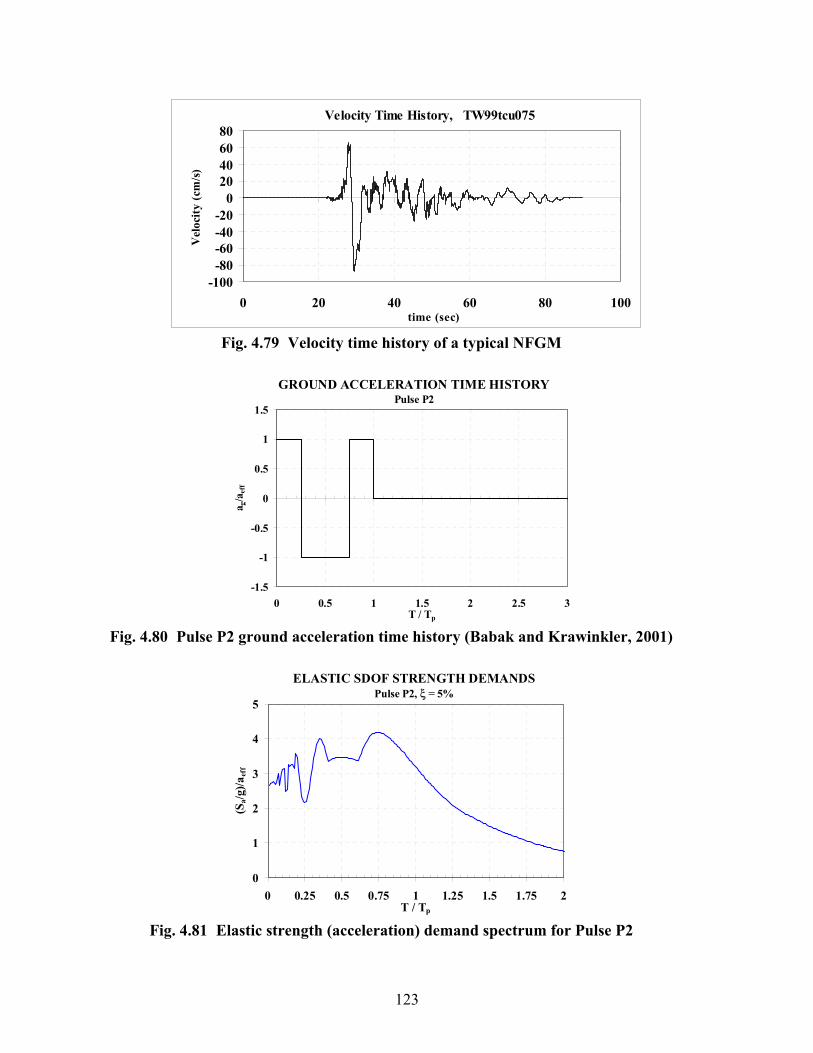
123

Velocity Time History, TW99tcu075

-100-80-60-40-20

020406080

0 20 40 60 80 100time (sec)

Vel

ocity

(cm

/s)

Fig. 4.79 Velocity time history of a typical NFGM

GROUND ACCELERATION TIME HISTORYPulse P2

-1.5

-1

-0.5

0

0.5

1

1.5

0 0.5 1 1.5 2 2.5 3T / Tp

a g/a

eff

Fig. 4.80 Pulse P2 ground acceleration time history (Babak and Krawinkler, 2001)

ELASTIC SDOF STRENGTH DEMANDSPulse P2, ξ = 5%

0

1

2

3

4

5

0 0.25 0.5 0.75 1 1.25 1.5 1.75 2T / Tp

(Sa/g

)/aef

f

Fig. 4.81 Elastic strength (acceleration) demand spectrum for Pulse P2

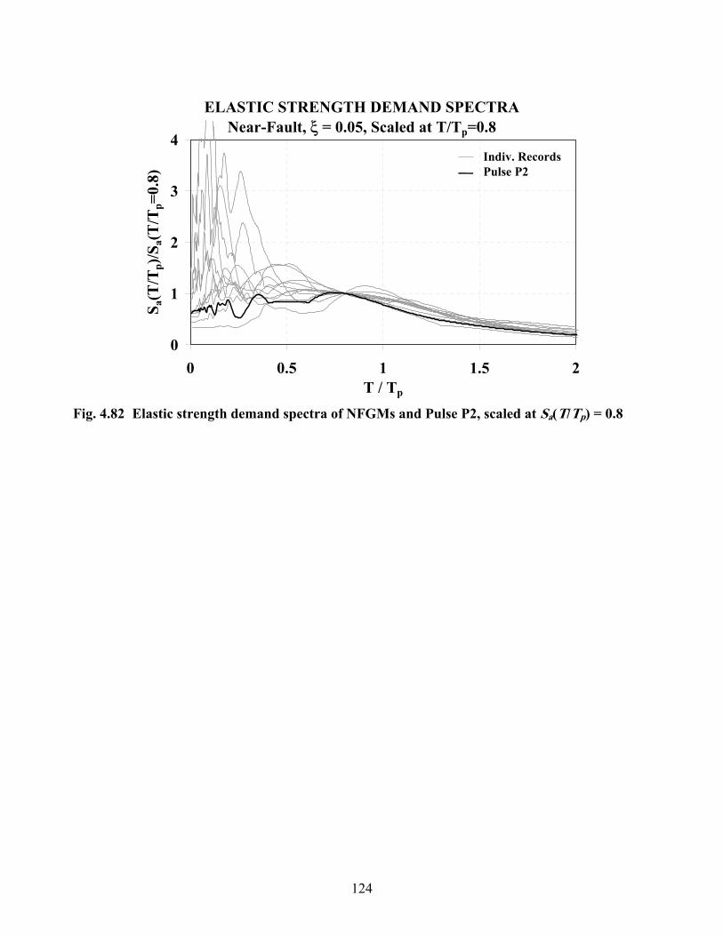
124

ELASTIC STRENGTH DEMAND SPECTRANear-Fault, ξ = 0.05, Scaled at T/Tp=0.8

0

1

2

3

4

0 0.5 1 1.5 2T / Tp

S a(T

/Tp)

/Sa(

T/T

p=0.

8)Indiv. RecordsPulse P2

Fig. 4.82 Elastic strength demand spectra of NFGMs and Pulse P2, scaled at Sa(T/Tp) = 0.8

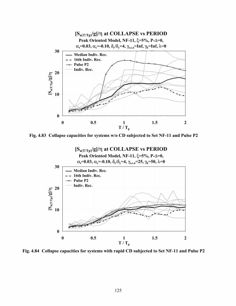
125

[Sa(T/Tp)/g]/η at COLLAPSE vs PERIODPeak Oriented Model, NF-11, ξ=5%, P-∆=0,

αs=0.03, αc=-0.10, δc/δy=4, γs,c,a=Inf, γk=Inf, λ=0

0

10

20

30

0 0.5 1 1.5 2T / Tp

[Sa(

T/T

p)/g

]/ ηMedian Indiv. Rec.16th Indiv. Rec.Pulse P2Indiv. Rec.

Fig. 4.83 Collapse capacities for systems w/o CD subjected to Set NF-11 and Pulse P2

[Sa(T/Tp)/g]/η at COLLAPSE vs PERIODPeak Oriented Model, NF-11, ξ=5%, P-∆=0,

αs=0.03, αc=-0.10, δc/δy=4, γs,c,a=25, γk=50, λ=0

0

10

20

30

0 0.5 1 1.5 2T / Tp

[Sa(

T/T

p)/g

]/ η

Median Indiv. Rec.16th Indiv. Rec.Pulse P2Indiv. Rec.

Fig. 4.84 Collapse capacities for systems with rapid CD subjected to Set NF-11 and Pulse P2

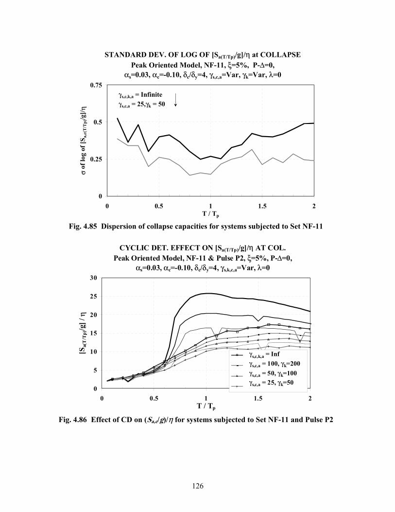
126

STANDARD DEV. OF LOG OF [Sa(T/Tp)/g]/η at COLLAPSEPeak Oriented Model, NF-11, ξ=5%, P-∆=0,


0

0.25

0.5

0.75

0 0.5 1 1.5 2T / Tp

σ of

log

of [S

a,c(

T/T

p)/g

]/ η

γs,c,k,a = Infiniteγs,c,a = 25,γk = 50

Fig. 4.85 Dispersion of collapse capacities for systems subjected to Set NF-11

CYCLIC DET. EFFECT ON [Sa(T/Tp)/g]/η AT COL.Peak Oriented Model, NF-11 & Pulse P2, ξ=5%, P-∆=0,

αs=0.03, αc=-0.10, δc/δy=4, γs,k,c,a=Var, λ=0

0

5

10

15

20

25

30

0 0.5 1 1.5 2T / Tp

[Sa(

T/T

p)/g

] / η

γs,c,k,a = Infγs,c,a = 100, γk=200γs,c,a = 50, γk=100γs,c,a = 25, γk=50

Fig. 4.86 Effect of CD on (Sa,c/g)/η for systems subjected to Set NF-11 and Pulse P2

127

CYCLIC DET. EFFECT ON [Sa(T/Tp)/g]/η AT COL.Peak Oriented Model, NF-11, ξ=5%, P-∆=0, αs=0.03, αc=-0.10, δc/δy=4, γs,k,c,a=Var, λ=0

0

5

10

15

20

0 0.5 1 1.5 2T / Tp

[Sa(

T/T

p)/g

] / η



0

0.2

0.4

0.6

0.8

1

1.2

0 0.5 1 1.5 2T / Tp

Var

iatio

n / B

ase

Cas

e



Fig. 4.87 Effect of CD on (Sa,c/g)/η for systems subjected to Set NF-11; δc/δy = 4, αc = -0.10


0

5

10

15

20

0 0.5 1 1.5 2T / Tp

[Sa(

T/T

p)/g

] / η γs,c,k,a = Inf

γs,c,a = 100, γk=200γs,c,a = 50, γk=100γs,c,a = 25, γk=50


0

0.2

0.4

0.6

0.8

1

1.2

0 0.5 1 1.5 2T / Tp

Var

iatio

n / B

ase

Cas

e



Fig. 4.88 Effect of CD on (Sa,c/g)/η for systems subjected to Set NF-11; δc/δy = 4, αc = -0.30

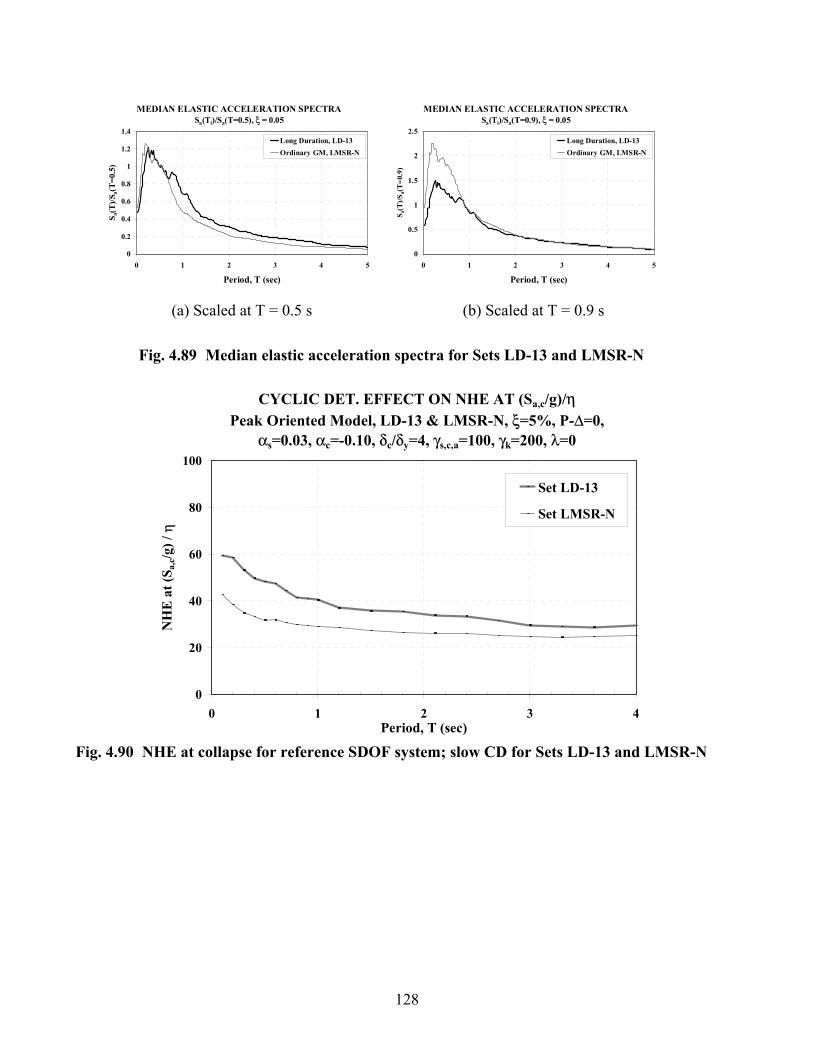
128

MEDIAN ELASTIC ACCELERATION SPECTRA Sa(Ti)/Sa(T=0.5), ξ = 0.05

0

0.2

0.4

0.6

0.8

1

1.2

1.4

0 1 2 3 4 5

Period, T (sec)

S a(T

)/Sa(

T=0.

5)

Long Duration, LD-13Ordinary GM, LMSR-N

MEDIAN ELASTIC ACCELERATION SPECTRA Sa(Ti)/Sa(T=0.9), ξ = 0.05

0

0.5

1

1.5

2

2.5

0 1 2 3 4 5

Period, T (sec)

S a(T

)/Sa(

T=0.

9)

Long Duration, LD-13Ordinary GM, LMSR-N

(a) Scaled at T = 0.5 s (b) Scaled at T = 0.9 s

Fig. 4.89 Median elastic acceleration spectra for Sets LD-13 and LMSR-N

CYCLIC DET. EFFECT ON NHE AT (Sa,c/g)/ηPeak Oriented Model, LD-13 & LMSR-N, ξ=5%, P-∆=0,


0

20

40

60

80

100


NH

E a

t (S a

,c/g

) / η

Set LD-13

Set LMSR-N

Fig. 4.90 NHE at collapse for reference SDOF system; slow CD for Sets LD-13 and LMSR-N

129

NHE AT (Sa,c/g)/η RATIOS FOR DIFF. GM SETSPeak Oriented Model, LD-13 & LMSR-N, ξ=5%, P-∆=0,


0

0.5

1

1.5

2


LD-1

3 / L

MSR

-N



Fig. 4.91 Ratios of NHE at collapse for reference SDOF system with different CD

rates, Sets LD-13 over LMSR-N

EFFECT OF CYCLIC DET. ON (Sa/g) / η AT COLLAPSEPeak Oriented Model, LD-13 & LMSR-N, ξ=5%, P-∆=0,


0

4

8

12

16


(Sa,

c/g) /

η


LD-13LMSR-N

Fig. 4.92 Effect of CD on (Sa,c/g)/η for systems subjected to sets of GM with

different strong motion duration

130

EFFECT OF CYCLIC DET. ON (Sa/g)/η AT COLLAPSEPeak Oriented Model, LD-13 & LMSR-N, ξ=5%, P-∆=0,


0

0.2

0.4

0.6

0.8

1

1.2


Var

iatio

n / B

ase

Cas

e


LD-13LMSR-N

Fig. 4.93 Effect of CD on median collapse capacity ratios for systems subjected to

sets of GM with different strong motion duration

EFFECT OF CYCLIC DET. ON (Sa/g)/η AT COLLAPSEBilinear Model, LD-13 & LMSR-N, ξ=5%, P-∆=0,


0

0.2

0.4

0.6

0.8

1

1.2


Var

iatio

n / B

ase

Cas

e


LD-13LMSR-N

Fig. 4.94 Effect of CD on median collapse capacity ratios for systems subjected to Sets

of GM with different strong motion duration, bilinear models

5 Global Collapse of MDOF Systems

5.1 INTRODUCTION

In MDOF structures collapse refers to the loss of ability to resist gravity loads. Collapse is local

if one or several components carrying vertical load fail without compromising the stability of the

whole system. Global collapse may occur by propagation of local collapses, often termed

“progressive collapse” (Liu et al. 2003; Kaewkulchai and Willamson, 2003). In this study, global

collapse implies dynamic instability in a side-sway mode, usually triggered by large story drifts

that are amplified by P-∆ effects and deterioration in strength and stiffness.

Several investigations have focused on the topic of global collapse due to P-∆ effects. For

instance, Bernal (1992) evaluated the safety against dynamic instability of two-dimensional non-

deteriorating frames based on the reduction of a multi-story building to an equivalent SDOF

system. The results indicated that the minimum base shear capacity needed to withstand a given

ground motion without collapse is strongly dependent on the shape of the controlling

mechanism. Gupta and Krawinkler (1999) evaluated the performance of steel moment-resisting

frames (MRFs) in the SAC project. They concluded that P-∆ effects could lead to global collapse

of the structures due to the development of a negative post-yielding stiffness in specific stories of

the frame. Medina (2002) reached the same conclusions by evaluating non-deteriorating generic

frames with different number of stories and different periods.

Most of the previous investigations of global collapse of MDOF systems focus on

geometric nonlinearities (P-∆ effects), but few systematic studies have taken into account

deterioration of strength and stiffness in the nonlinear range. Two exceptions are the works of

Lee and Foutch (2001) and Jalayer (2003) (see Chapter 2). In this chapter, global collapse of

generic frames is evaluated for systems including nonlinear behavior by means of concentrated

plasticity. The building models utilize rotational springs that include deterioration of strength in

the backbone curve and cyclic deterioration. The procedure for evaluating collapse capacity is

132

similar to that implemented for SDOF systems, i.e., the relative intensity is increased until the

relative intensity–EDP curve becomes horizontal. The collapse capacity is expressed in terms of

the maximum relative intensity the frame can withstand prior to collapse.

5.2 COLLAPSE CAPACITY OF MDOF SYSTEMS

The general procedure for computing collapse capacity has been described in Section 2.3. Global

collapse is obtained by increasing the relative intensity, [Sa(T1)/g]/γ, of the structure until the

response of the system becomes unstable. Sa(T1) is a measure of the intensity of the ground

motion and corresponds to the 5% damped spectral acceleration at the fundamental period of the

structure, without P-∆ effects. γ is a measure of the strength of the structure and is equivalent to

the base shear coefficient12, γ = Vy/W, where Vy is the yield base shear without P-∆ effects and W

is the weight of the structure.

[Sa(T1)/g]/γ represents the ductility dependent response modification factor, which in

present codes is equal to the R-factor if no overstrength is present. [Sa(T1)/g]/γ may be

interpreted in two ways; either keeping the ground motion intensity constant while decreasing

the base shear strength of the structure (the R-factor perspective), or keeping the base shear

strength constant while increasing the intensity of the ground motion, i.e., the IDA perspective13

(Vamvatsikos and Cornell, 2002).

In MDOF structures, the threshold of inelastic behavior is not uniquely related to the

intensity measure, Sa(T1), because the higher-mode effects are not included in the IM. Therefore,

to assure elastic behavior for the lowest relative intensity, the selected initial relative intensity is

chosen as [Sa,c(T1)/g]/γ = 0.25. Since only bending elements are utilized in the generic frames

(i.e., shear and axial failures are not modeled), collapse implies that the interstory drift in a

specific story grows without bounds (incremental collapse), i.e., the [Sa(T1)/g]/γ - EDP curve

becomes horizontal (Fig. 2.1). This large EDP increase with a minute increase in the relative

intensity is associated with a state (not a mechanism in the classical sense) in which P-∆ effects

become equal to the first-order story shear resistance provided by the structural elements.

12 The nomenclature for the base shear coefficient (γ) should not be confused with that of the cyclic deterioration parameter γs,c,k,a. 13 The dual interpretation is not correct if gravity moments are a major portion of the plastic moment capacity of the beams, and/or there are considerable changes in column axial forces due to overturning moments, as compared to the gravity induced axial forces in columns.

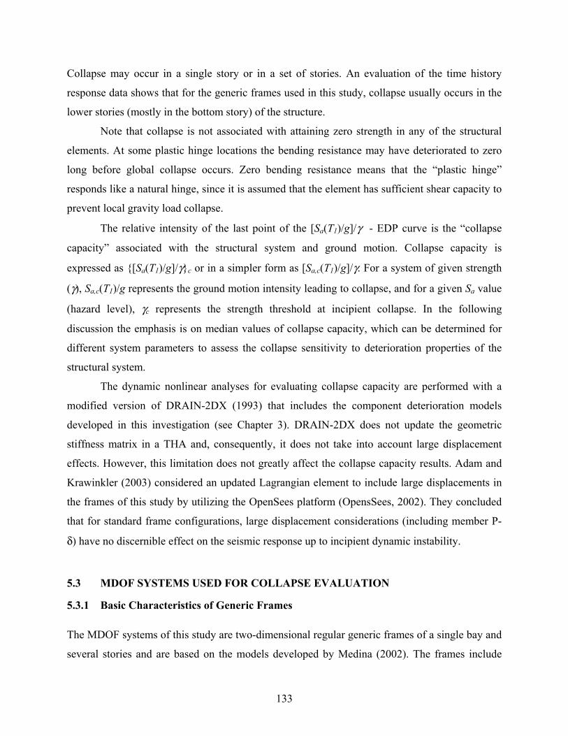
133

Collapse may occur in a single story or in a set of stories. An evaluation of the time history

response data shows that for the generic frames used in this study, collapse usually occurs in the

lower stories (mostly in the bottom story) of the structure.

Note that collapse is not associated with attaining zero strength in any of the structural

elements. At some plastic hinge locations the bending resistance may have deteriorated to zero

long before global collapse occurs. Zero bending resistance means that the “plastic hinge”

responds like a natural hinge, since it is assumed that the element has sufficient shear capacity to

prevent local gravity load collapse.

The relative intensity of the last point of the [Sa(T1)/g]/γ - EDP curve is the “collapse

capacity” associated with the structural system and ground motion. Collapse capacity is

expressed as {[Sa(T1)/g]/γ}c or in a simpler form as [Sa,c(T1)/g]/γ. For a system of given strength

(γ), Sa,c(T1)/g represents the ground motion intensity leading to collapse, and for a given Sa value

(hazard level), γc represents the strength threshold at incipient collapse. In the following

discussion the emphasis is on median values of collapse capacity, which can be determined for

different system parameters to assess the collapse sensitivity to deterioration properties of the

structural system.

The dynamic nonlinear analyses for evaluating collapse capacity are performed with a

modified version of DRAIN-2DX (1993) that includes the component deterioration models

developed in this investigation (see Chapter 3). DRAIN-2DX does not update the geometric

stiffness matrix in a THA and, consequently, it does not take into account large displacement

effects. However, this limitation does not greatly affect the collapse capacity results. Adam and

Krawinkler (2003) considered an updated Lagrangian element to include large displacements in

the frames of this study by utilizing the OpenSees platform (OpensSees, 2002). They concluded

that for standard frame configurations, large displacement considerations (including member P-

δ) have no discernible effect on the seismic response up to incipient dynamic instability.

5.3 MDOF SYSTEMS USED FOR COLLAPSE EVALUATION

5.3.1 Basic Characteristics of Generic Frames

The MDOF systems of this study are two-dimensional regular generic frames of a single bay and

several stories and are based on the models developed by Medina (2002). The frames include

134

rotational springs with deterioration in strength and stiffness. Their basic characteristics are the

following:

• The frames have six different number of stories, N = 3, 6, 9, 12, 15, and 18 (Fig. 5.1).

• The fundamental period of the structure is associated with the number of stories. “Stiff

frames” have a fundamental period T1 = 0.1N, whereas “flexible frames” have T1 = 0.2N.

These values are considered to be reasonable lower and upper boundaries for moment-

resisting frames. The overlap of the fundamental periods at T1 = 0.6 s, 1.2 s, and 1.8 s

allows assessing of the effects of N on the response.

• The same moment of inertia is assigned to the columns in a story and the beam above

them.

• Relative element stiffnesses are tuned to obtain a straight line deflected shape for the

first mode. Absolute stiffnesses are tuned to obtain the aforementioned periods.

• The strength design of the frames is such that simultaneous yielding is attained under a

parabolic load pattern (NEHRP, k = 2).

• Centerline dimensions are used for all elements.

• The ratio of span to story height is 2.0.

• The same mass is used at all floor levels.

• The effect of gravity load moments on plastic hinge formation is not included.

• Global P-∆ is included, whereas member P-δ is disregarded. The mass used to consider

P- ∆ effects is 1.4 times larger than the seismically effective mass. That is to say, P is the

dead load plus a live load equal to 40% of the dead load.

• Axial deformations and P-M-V interaction are not considered.

• Soil-structure interaction is neglected.

• For nonlinear dynamic analyses, 5% Rayleigh damping is assigned to the first mode and

to the mode at which the cumulative mass participation exceeds 95%.

• Gravitational loads are applied at the beginning of the time history. The geometric

stiffness matrix (Kg) is then calculated, added to the elastic stiffness matrix (Ke) and kept

constant throughout the time history.

• Failure modes: In most cases, the strong column–weak beam philosophy is considered

and the columns are modeled with infinite strength (BH frames) (Fig. 5.2). In Section 5.6

the columns are modeled with finite strength (BH-CH, i.e., beam hinge model with

135

possible yielding of columns). Springs are added to the ends of all the columns to permit

plastic hinging in the columns. A weak first-story mechanism (WS) is also modeled.

Appendix B provides more information on the basic characteristics of the generic frames.

5.3.2 Deteriorating Characteristics of Plastic Hinge Springs of Generic Frames

To obtain a consistent evaluation of collapse capacity, the same deteriorating hysteretic model is

assumed at every plastic hinge of the generic frames. A set of reference frames14 with rotational

springs of intermediate ductility is used as a starting point. In these frames, the parameters for the

moment-rotation relationship at the ends of the members are as follows:

• Strain-hardening stiffness, αs,mem = 0.03 Ke

• Small post-capping stiffness, αc,mem = -0.1 Ke

• Medium ductility capacity, (δc/δy),mem = 4

• No cyclic deterioration (CD), (γs,c,k,a)mem = infinite

• Peak-oriented hysteretic model

For reasons described in Appendix B, the elastic stiffness of members with concentrated

plasticity is divided into the elastic stiffness of the rotational springs at the end of the member

and the elastic stiffness of the beam-column element. Independently of these internal

manipulations, the properties of the “springs” in the rest of this chapter refer to the moment-

rotation relationship at the end of the member. The nomenclature is simplified and, for instance,

αc,mem becomes αc.

For assessing the effect of different parameters, each parameter is varied individually

while holding all others constant. The selection of parameters to be evaluated is primarily based

on the results of the parametric study of SDOF systems. Parameters that do not have a large

effect on the collapse capacity of SDOF systems are disregarded, i.e., residual strength and the

level of pinching (κf,d). The emphasis is on those parameters that produce larger modifications to

collapse capacity:

14 A “set of frames” refers to the group of frames of 3, 6, 9, 12, 15, and 18 stories for T1 = 0.1N and T1 = 0.2N that share common characteristics in the springs of the members.

136

Post-capping stiffness ratio, αc = -0.1, -0.3, and -0.5.

• Ductility capacity, δc/δy = 2, 4, and 6.

• Cyclic deterioration, γs,c,k,a = 25, 50, 100 and infinite.

• Hysteretic models. Peak-oriented, pinching, and bilinear models.

Table 5.1 shows the sets of generic frames analyzed. Note that it includes a set of frames

in which the variation is not related to the springs but to the P-∆ effects (cases 3 and 14).

5.3.3 Set of Ground Motions

The parametric study utilizes the set of 40 GMs used for SDOF systems, LMSR-N (Section

4.2.3). The intensity measure is the 5% damped spectral acceleration at the first mode period of

the structure, Sa(T1). This choice implies that the frequency content of the ground motion cannot

be considered explicitly and that the fundamental period of the structure is known. For this

reason, the dispersion in the response depends on the importance of higher mode effects (scatter

for T < T1) and on the extent of inelasticity, which leads to period elongation (scatter for T > T1).

Sections 5.4–5.7 summarize the salient findings for generic frames. The titles of the

presented figures contain the following additional information as compared with the titles for

SDOF systems: number of stories of the frame (N), and failure mechanism (BH, BH-CH (see

Section 5.3.1). A four-digit code is used for identifying the generic frames. The first two digits

correspond to the number of stories and the other two to the first mode period. For instance, 0918

means a 9-story frame with T1 = 1.8 s.

5.4 EDPS FOR GENERIC FRAMES WITH INFINITELY STRONG COLUMNS

5.4.1 Effect of Deterioration Parameters on EDPs

The assessment of several EDPs prior to collapse provides information on the effect of

deterioration parameters on the response. The EDPs analyzed are:

• Normalized maximum roof drift angle, ]/)(/[ 1max, HTSdrθ , where H is the total height of

the frame

• Normalized maximum story drift over the height, ]/)(/[ 1max, HTSdsθ

• Normalized maximum story drift profiles, ]/)(/[ 1max, HTSdsiθ

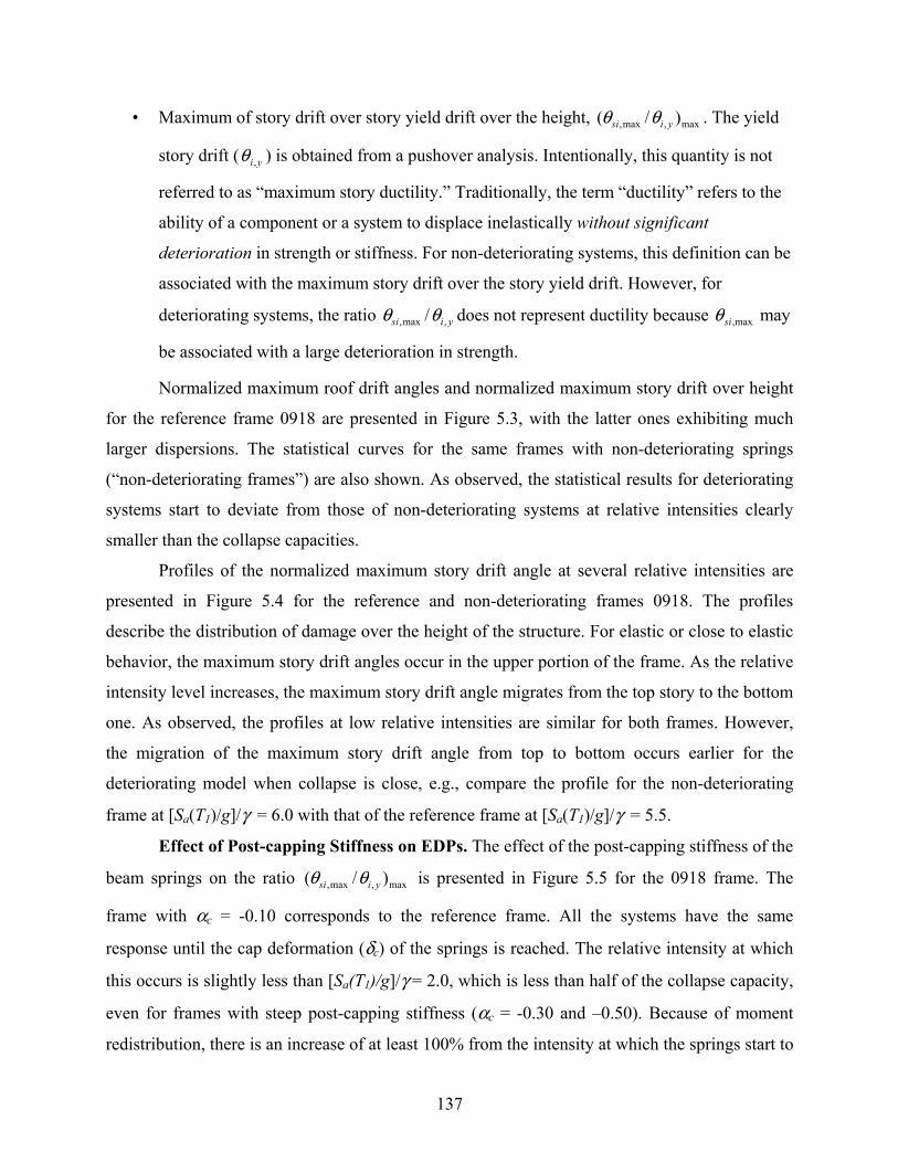
137

• Maximum of story drift over story yield drift over the height, max,max, )/( yisi θθ . The yield

story drift ( yi,θ ) is obtained from a pushover analysis. Intentionally, this quantity is not

referred to as “maximum story ductility.” Traditionally, the term “ductility” refers to the

ability of a component or a system to displace inelastically without significant

deterioration in strength or stiffness. For non-deteriorating systems, this definition can be

associated with the maximum story drift over the story yield drift. However, for

deteriorating systems, the ratio yisi ,max, /θθ does not represent ductility because max,siθ may

be associated with a large deterioration in strength.

Normalized maximum roof drift angles and normalized maximum story drift over height

for the reference frame 0918 are presented in Figure 5.3, with the latter ones exhibiting much

larger dispersions. The statistical curves for the same frames with non-deteriorating springs

(“non-deteriorating frames”) are also shown. As observed, the statistical results for deteriorating

systems start to deviate from those of non-deteriorating systems at relative intensities clearly

smaller than the collapse capacities.

Profiles of the normalized maximum story drift angle at several relative intensities are

presented in Figure 5.4 for the reference and non-deteriorating frames 0918. The profiles

describe the distribution of damage over the height of the structure. For elastic or close to elastic

behavior, the maximum story drift angles occur in the upper portion of the frame. As the relative

intensity level increases, the maximum story drift angle migrates from the top story to the bottom

one. As observed, the profiles at low relative intensities are similar for both frames. However,

the migration of the maximum story drift angle from top to bottom occurs earlier for the

deteriorating model when collapse is close, e.g., compare the profile for the non-deteriorating

frame at [Sa(T1)/g]/γ = 6.0 with that of the reference frame at [Sa(T1)/g]/γ = 5.5.

Effect of Post-capping Stiffness on EDPs. The effect of the post-capping stiffness of the

beam springs on the ratio max,max, )/( yisi θθ is presented in Figure 5.5 for the 0918 frame. The

frame with αc = -0.10 corresponds to the reference frame. All the systems have the same

response until the cap deformation (δc) of the springs is reached. The relative intensity at which

this occurs is slightly less than [Sa(T1)/g]/γ = 2.0, which is less than half of the collapse capacity,

even for frames with steep post-capping stiffness (αc = -0.30 and –0.50). Because of moment

redistribution, there is an increase of at least 100% from the intensity at which the springs start to

138

deteriorate in strength to the intensity at which collapse occurs. This behavior is not observed in

SDOF systems with steep αc, where collapse occurs soon after the peak strength is reached. The

ratios max,max, )/( yisi θθ for systems with αc = -0.30 and –0.50 are very similar, a common

phenomenon when comparing systems with steep negative slopes.

The ratios max,max, )/( yisi θθ at which the curves start to deviate from each other is about

2.5. As expected, this value is smaller than the ductility capacity of the rotational springs because

not all of the springs yield at the same time.

Effect of Component Ductility Capacity on EDPs. Figure 5.6 shows max,max, )/( yisi θθ

ratios for frames 0918 that have different ductility capacity in the rotational springs but the same

αc = -0.10. The frame with δc/δy = infinite corresponds to the non-deteriorating one, whereas the

system with δc/δy = 4 is the reference case. Variations in the ductility capacity of the beam

springs produce differences in the median response at 0.2/]/)([ 1 <γgTSa .

Effect of Cyclic Deterioration on EDPs. Figure 5.7 presents the effect of CD on the

ratios max,max, )/( yisi θθ . The frames have springs with δc/δy = 4, αc = -0.10 and different rates of

CD. The story ductilities over the height for the non-deteriorating frame are also displayed. For

frames with springs having finite γs,c,k,a values, the curve γθθ /]/)([)/( 1max,max, gTSayisi − deviates

from that of the non-deteriorating frame before the peak-strength of the springs is attained.

However, the effect becomes significant only after the peak strength is surpassed.

5.4.2 Global Pushover Curves for Deteriorating Systems

The pushover method estimates force and deformation demands using a static incremental,

inelastic analysis (Lawson et al., 1994; Krawinkler and Seneviratna, 1998). In this work, the

method is used to study the behavior of deteriorating systems.

Figure 5.8 presents a comparison of global pushover curves for the non-deteriorating and

the deteriorating reference frame 0909 when a parabolic lateral load pattern (NEHRP, k = 2) is

applied to the system. For both systems the global strain-hardening stiffness is larger than in the

beam springs (αs = 0.04 vs. 0.03). For the deteriorating system the global “ductility capacity”

(drift at onset of deterioration divided by yield drift) is smaller (3.0 vs. 4.0) and the global post-

capping stiffness is steeper (αc = -0.34 vs. –0.10) than in the beam springs. Also, for large

139

deformations there is a third post-yielding branch that indicates an apparent “recovery” in the

stiffness of the global pushover curve. These observations deserve explanation.

One contributor to these differences is the fact that columns remain elastic throughout the

pushover analysis. Thus, initial displacements, which define the elastic stiffness, come from

elastic contributions of beams and columns. After the simultaneous yielding of the beam springs

in the pushover analysis (because of the assumptions discussed previously), the incremental

displacements in the global pushover curve contain deformations from beams (beam elastic

deformations and plastic hinge spring deformations), and elastic deformations from columns.

These elastic deformations in columns account for the increase in the effective αs, part of the

increase in αc, and the decrease in δc/δy of the global pushover curve.

There is an additional phenomenon of inelastic redistribution that may affect the

pushover curve (and dynamic time history results) at large inelastic deformations. If P-∆ effects

are small and no strength deterioration occurs, the generic frames are expected to take on a

deflected shape close to a straight line under a parabolic load pattern, regardless of the level of

displacement. This is illustrated in Figure 5.9a for the non-deteriorating 1818 frame. This does

not hold true when P-∆ effects are important (i.e., when they lead to a negative story tangent

stiffness); see the deflection profiles of the 1836 frame in Figure 5.9b. In this frame the P-∆

effect amplifies the story drifts in the lower stories, which results in highly nonlinear deflected

shapes with very large drifts in the lower stories and unloading (decrease in story drifts) in the

upper stories.

Post-capping strength deterioration has a similar effect as P-∆. Figure 5.10 shows

deflected shapes associated with the roof drifts indicated with dotted vertical lines in Figure 5.8.

Without post-capping strength deterioration, the deflected shapes remain essentially linear even

though P-∆ (which is small for the 0909 frame) is included (Fig. 5.10a). When strength

deterioration is included, the deflection profiles acquire a very different shape with great

amplifications of drifts in the lower stories (Fig. 5.10b). This radical change in deflected shape

occurs when the loading path is on the descending branch of the pushover curve. This change in

deflected shape is the main reason for the difference between the αc = -0.10 of the component

model and the effective αc = -0.34 seen in the global pushover.

The same phenomenon also accounts for the “recovery” portion of the pushover curve at

very large drifts. This recovery portion comes from the fact that the lower portion of the frame

140

has undergone very large horizontal displacements and the global bending mode (i.e., the

cantilever bending mode) of the infinitely strong columns starts to dominate over the effect of

frame action. This is illustrated in Figures 5.11–5.12.

Figure 5.11 shows moment-rotation diagrams for beams at each floor level, from zero

load to three load points, which are indicated in Figure 5.8 as “A,” “B,” and “C.” At load point A

(δr/δyr = 3.1, beginning of deterioration), all springs at the beam ends, bottom to top, as well as at

the column base, are close to their capping points [(δc/δy)elem = 4] and the deflected shape is still

close to linear. As the roof displacement increases further, the beams close to the bottom of the

structure undergo large rotations and deteriorate rapidly in strength whereas the beams close to

the top unload (since the lateral loads on the frame decrease). At point B (δr/δyr = 5.3) the

column springs at the base and the second-story beam springs are at zero strength, and the global

resistance of the structure has deteriorated to about 0.4V/Vy. As the roof displacement is

increased further, the springs at level 3 lose all their resistance and beam-moment deterioration

propagates upward in the structure. This is also reflected in the deflection profiles of Figure 5.10.

Despite the complete loss of resistance in the bottom level springs, the structure still has

some lateral resistance left because of the global bending strength of the columns. Only the

strength at the column base is capped and subjected to deterioration, whereas the columns at all

other locations have infinite strength. The moment–roof drift relationships of Figure 5.12

illustrate the transfer of resistance to the columns. In the first story, both the base of the columns

and the beam reach their bending capacities and thereafter their strength deteriorates to zero,

whereas the first-story column moment at level 2 (where the strength is infinite) increases even

after the column base starts to deteriorate in strength. For lower-story columns, once the

associated beam starts to deteriorate in strength, the column moment at the top of the story

increases, whereas the column moment at the bottom of the same story decreases and reverses

direction, taking large values opposite to the direction of frame action. Thus, for very large

displacements the columns in the lower stories go into single curvature with large moments at

both ends, i.e., the column acts more as a multi-story cantilever than a column in a moment-

resisting frame. This observation has been reported elsewhere (Gupta and Krawinkler, 1999;

Medina, 2002).

As can be seen from Figure 5.12, the column moments can become very large compared

to the value when the beam reaches its bending strength. The implication is that the strong

column–weak beam factor would have to be very large (larger than 3.0) in order to avoid column

141

plastic hinges at very large lateral displacements. The strong columns are responsible also for the

stiffness recovery in the late stages of the global pushover curve shown in Figure 5.8. It is likely

that such strong columns do not exist in actual frame structures, which makes the data presented

here somewhat hypothetical. They are represented to evaluate and explain behavior from a

mechanics perspective, but they have no significant bearing on the results presented for collapse

capacities. The very large column moments occur at very large drifts, and an evaluation of the

collapse capacities has disclosed that at these large drifts almost all IDAs have close to a

horizontal slope, i.e., these phenomena dominate only close to collapse. The effect of limited

column bending strength is discussed separately in Section 5.6.

5.4.3 De-Normalized EDPs

To illustrate “realistic” values for collapse capacities and associated drifts, the [Sa,c(T1)/g]/γ −

EDP curves of the type shown in Figure 5.4 are de-normalized for several reference frames by

assuming a base shear strength γ = 0.6, 0.6, 0.4, and 0.2 for periods of T1 = 0.3, 0.6, 0.9, and 1.8

s, respectively.

Figures 5.13–5.14 present IDAs for maximum roof drift angle [Sa(T1)/g−θr,max] for the

reference frames 0303, 0306, 0909, and 0918. Note that most of the individual IDAs become

almost horizontal at relatively small roof drifts, i.e., the large collapse roof drifts reported in the

SAC studies (FEMA 350, 2000) are not observed here. One reason is that the elastic period of

the SAC structures is even longer than that of the “flexible” structures used here, i.e., the yield

drifts of the SAC structures are somewhat larger. However, most of the difference is attributed to

the representation of component moment-rotation relationships using more realistic deterioration

models in this study. Observe that the median EDP curves give the impression that the intensity

increases at a rather high rate until the median curve terminates. This is not observed in the IDAs

of individual records in which the rate of increase in intensity becomes small much earlier.

The figures also include the global pushover curves for each frame. The base shear

strength of the global pushover curve is normalized by the inverse of the effective mass

coefficient of the first mode to obtain an approximate correlation with Sa(T1). The correlation is

not exact in the elastic range due to the effect of higher modes in the response. For the 9-story

frames, the onset of the third post-yielding branch of the global pushover curves approximately

142

coincides with the EDP region in which most of the individual curves become flat, and could be

considered as an indication of the roof drift at which collapse occurs.

Figure 5.15 presents the variation with relative intensity of the median θs,max /θr,max ratio

for several reference frames. This information can be used to estimate the maximum interstory

drift based on the IDAs of Figures 5.13–5.14. For instance, for the 0918 frame of Figure 5.15, for

which the individual IDAs become horizontal around a roof drift of 0.04, the associated

maximum story drift is on the order of 08.004.02 =x .

5.5 COLLAPSE CAPACITY OF GENERIC FRAMES WITH INFINITELY STRONG COLUMNS

5.5.1 Collapse Capacity for the Set of Reference Frames

Figure 5.16 shows median and 16th percentile collapse capacity spectra for the set of reference

frames. Collapse capacities are grouped in stiff (T1 = 0.1N) and flexible (T1 = 0.2N) frames. The

collapse capacity strongly depends on the first mode period T1. This is expected for the short-

period structure with T1 = 0.3 s, where the collapse capacity is much smaller than that for T1 =

0.6 s. But the large decrease in collapse capacity for long-period structures is striking, indicating

that the “period independent R-factor concept” may be way off for long-period structures, i.e., it

would be non-conservative to assume that R is independent of T. The reason is the P-∆ effect,

which is more important than might be expected.

The sensitivity to the number of stories is analyzed by comparing collapse capacity

spectra for flexible and stiff frames with the same fundamental period (Fig. 5.16). In a vertical

comparison, the frames have the same fundamental period and a different number of stories, e.g.,

0306 and 0606. In the period range between T = 0.6 s and 1.5 s frames with more stories have

larger collapse capacities for the same fundamental period. One of the reasons for this pattern is

that frames with more stories have smaller P-∆ effects. However, the differences are 15% at most

and for long fundamental periods the trend may be reversed (see frames 0918 and 1818), likely

because of higher-mode effects or different influences of deterioration parameters on collapse

capacities.

The effect of P-∆ is also appreciated in Figure 5.17, which shows collapse capacities

versus the number of stories for flexible and stiff frames. Except for short-period frames,

collapse capacities of stiff frames are larger (especially at long periods) because P-∆ effects are

143

smaller for these frames. The trend is reversed for the three-story frames because P-∆ effects are

small and the displacements are more sensitive to the strength of the system, causing the

structure with shorter fundamental period to have the smaller collapse capacity.

5.5.2 Effect of Post-Capping Stiffness on Collapse Capacity

The effect of the post-capping stiffness is isolated in Figure 5.18a, which shows median collapse

capacities for frames similar to the reference frame but with different αc values. There is a large

difference between the collapse capacities for systems with αc = -0.1 and -0.3. However, if αc

represents a steep slope, any further increase in slope has only a small effect because the

component reaches zero strength soon after δc is reached. Figure 5.18b presents the collapse

capacity ratios with respect to the most ductile system (the reference frame). The larger

differences arise in the medium-period range, where ratios smaller than 0.7 are reported. This

information may be compared with the ratios of Figure 4.12b, which presents collapse capacity

ratios for SDOF systems with the same hysteretic properties as those of the springs at the beam

ends of the frames. Although the P-∆ effects are not properly represented in the SDOF systems,

the effect of post-capping stiffness on collapse capacity of SDOF and MDOF systems is

comparable.

Figure 5.18c shows the dispersion in collapse capacity due to RTR variability in terms of

the standard deviation of the log of [Sa,c(T1)/g]/γ. The dispersion is not sensitive to the

fundamental period of the frame and, although rather large, is smaller than that of the SDOF

systems with the same hysteretic properties as the springs at the beam ends (Fig. 4.19a). The

dispersion of collapse capacity is not greatly affected by changes of the αc value of the springs of

the reference frame. The same conclusion is obtained when the ductility capacity and the CD

parameters are modified.

5.5.3 Effect of Ductility Capacity on Collapse Capacity

The effect of ductility capacity (δc/δy) on the median collapse capacity is illustrated in Figure

5.19a for systems with αc = -0.10. The effect of δc/δy is significant and, as observed in the

collapse capacity ratios of Figure 5.19b, essentially independent of the fundamental period of the

structure or the number of stories of the frame. The collapse capacity ratios may be compared

144

with those of the SDOF system with the same hysteretic characteristics of the springs of the

frames (Fig. 4.23b). The same trends are observed, although the ratios of the generic frames are

slightly larger (closer to 1.0), indicating a smaller effect in the MDOF systems.

Figure 5.20 presents the effect of δc/δy for systems with αc = -0.30. The steeper post-

capping slope reduces the collapse capacities but increases the effect of δc/δy because collapse

occurs relatively soon after δc is reached. That is to say, a larger proportion of the collapse

capacity must be developed before the peak strength is surpassed.

5.5.4 Effect of Cyclic Deterioration on Collapse Capacity

Figure 5.21 illustrates the effect of CD on the collapse capacity of frames similar to the reference

one but with different CD rates in the springs. The effect of CD is evident, although not

overpowering, indicating that the combination of ductility capacity and post-capping stiffness is

more important than the CD effect. The effect diminishes for long-period structures because of

the dominant importance of P-∆ effects. Collapse capacity ratios of Figure 5.21b may be

compared with those of Figure 4.28b for an SDOF system with the same hysteretic

characteristics of the springs at the ends of the beams. It is observed that CD effects are larger for

SDOF systems because these do not have redistribution capabilities.

The utilized set of GMs (LMSR-N) includes records with relatively short strong motion

duration. However, according to the study of long-duration records for SDOF systems (Section

4.4.5), a large increase in the effect of CD on collapse capacity is not expected if a set of records

with longer strong motion duration is used. Thus, CD appears to be an important but not

dominant issue for collapse evaluation, unless the energy-dissipation capacity of the structural

components is very small (γ = 25).

5.5.5 Effect of Hysteretic Models on Collapse Capacity

Figure 5.22 shows collapse capacity spectra for frames with peak-oriented, pinching, and bilinear

models in the plastic hinge springs. The results indicate that frames with peak-oriented and

pinching models have similar collapse capacities. On the other hand, the relative collapse

capacities of frames with bilinear models present the same patterns as observed in SDOF

systems. For MDOF systems with very small fundamental period the collapse capacity of frames

145

with bilinear springs is slightly larger than that of frames with peak-oriented or pinching springs.

However, for frames with medium and long fundamental periods the trend reverses because the

branch with negative slope in the plastic hinge springs has a larger “ratcheting” effect in bilinear

models (Section 4.3.7).

5.5.6 Effect of P-∆ Effects on Collapse Capacity

Present engineering approaches have the potential to underestimate P-∆ effects, particularly for

long-period structures where the elastic story stability coefficient (θe) severely undervalues the

P-∆ effect in the inelastic range. In most practical cases the lower stories experience large drifts

when the structure undergoes large inelastic deformations, and the story stability coefficient

increases correspondingly.

P-∆ effects may produce collapse of the structures even without the inclusion of material

deterioration. Figure 5.23 presents global pushover curves for the reference frame 1836 with and

without including P-∆ effects. As observed, different stability coefficients exist for the elastic

( eθ ) and inelastic ranges ( iθ ). Figure 5.24a presents these coefficients for the generic frames.

Both the elastic and the inelastic stability coefficients increase with the number of stories and

depend on the strain hardening of the nonlinear elements, which for this study is 3% 15. For stiff

frames, eθ and iθ practically overlap, but for flexible frames with a large number of stories iθ

can be much larger than eθ . As a result of the increase in both coefficients with the number of

stories, the flexible frames of 9, 12, 15, and 18 stories exhibit a negative post-yield stiffness due

to structure P-∆ effects (Fig. 5.24b). This negative post-yielding stiffness can be associated with

eventual collapse of the frame under large relative intensities, even if non-deteriorating models

are used. Note that the non-deteriorating frame 1818 does not exhibit a negative slope. As shown

below, this frame does not collapse due to P-∆, unlike non-deteriorating frames 0918 and 1836.

This illustrates that the magnitude of P-∆ effects cannot be linked to some particular

characteristic of the system such as the fundamental period or the number of stories.

Figure 5.25 presents median collapse capacities for the reference and for the non-

deteriorating set of flexible frames. For non-deteriorating frames, collapse is caused solely by P- 15 The strain-hardening coefficient of the global pushover curve ( 0,sα ) is larger than 3% because the columns of the frame remain elastic.

146

∆ effects. As observed, for the 9-story frames (T1 = 1.8 s) the collapse capacity of the non-

deteriorating system is more than three times larger than that of the reference frame. However,

for the 18-story frames (T1 = 3.6 s.), P-∆ effects overpower the effect of material deterioration,

and the collapse capacity of the non-deteriorating frame is only 40% larger than that of the

reference frame. For non-deteriorating frames, the potential of collapse exists if the slope of the

post-yielding slope in the global pushover curve is negative. Observe the strain-hardening slope

of global pushover curves (Fig. 5.24b) and collapse capacities of non-deteriorating frames (Fig.

5.25).

To show the effect of P-∆ on collapse capacity, Figure 5.26 presents collapse capacities

for the set of reference frames without and with P-∆ effects. As expected, the effects of P-∆ on

collapse capacity are very large for long-period flexible structures. However, the important

observation is that the effects of P-∆ on collapse capacity apparently are also very large for

medium and even short period structures in which both the elastic and inelastic stability

coefficients are small (Fig. 5.24a). The reason is that components of deteriorating structures have

a range of post-capping negative tangent stiffness, which leads to a negative story and global

tangent stiffness range, which in turn is amplified (steeper) by even small P-∆ effects. This is

evident in the global pushover curves of Figure 5.27, which shows global pushover curves

without and with consideration of P-∆ for the 1212 reference frame. If P-∆ is ignored in the

analysis, the ratcheting effect in the negative stiffness range is greatly reduced and very large

displacements can be achieved without collapse. The consequence is a very large overprediction

of the collapse capacity. The conclusion is that any realistic prediction of collapse capacity must

incorporate P-∆ effects.

1.1 5.6 RESULTS FOR GENERIC FRAMES WITH COLUMNS OF FINITE STRENGTH

The generic frames evaluated in previous sections include infinitely strong columns, an

assumption that may lead to demands in the columns several times larger than those of the

beams. This condition can be quantified by means of the maximum “strong column factor”

(SCF), which for beam-hinge frames can be defined as the sum of the maximum moment

demands of the columns framing into a joint divided by the sum of the plastic moment capacity

of the beams framing into the joint. For single-bay generic frames, the SCF at any joint is equal

147

to (2Mc/Mp,b)max, where pbM , is the bending strength of the beam, and Mc is the largest column

moment demand occurring during the THA). Figure 5.28 shows maximum SCF over the height

for the stiff 9-story reference frame, revealing that close to collapse the median SCF is on the

order of 3 or more. These values establish an upper bound because they are based on the

maximum negative or positive moment of the columns that frame into the joint. The fact that the

SCF increases with the intensity of the GM is in accordance with results reported by Nakashima

and Sawaizumi (2000) and by Medina (2002).

In practical cases the column strength is limited, even if the strong column–weak beam

philosophy is utilized. To evaluate the collapse capacity when the columns yield before reaching

the large demands displayed in Figure 5.28, the column strengths of selected frames have been

tuned, taking as reference Section 21.4.2.2 of ACI 318-02 (2002). This section establishes that

for reinforced concrete members framing into a joint, ∑∑ ≥ gc MM 2.1 , where ∑ cM is the

sum of the moment capacity of the columns framing into the joint and ∑ gM is the sum of the

moment capacity of the beams. The frames that are designed with the strong column–weak beam

philosophy with the possibility of yielding in the columns are denoted as BH-CH models, and are

classified as follows:

(a) Frames with columns of “high strength”: ∑∑ = gc MM 4.2 , i.e., the strength of the

columns is twice the minimum ACI guidelines ( gc MM 2.1= for the generic single-bay

frames);

(b) Frames with columns of “intermediate strength”: ∑∑ = gc MM 2.1 , i.e., minimum

strength ACI requirements ( gc MM 6.0= for the generic frames); and

(c) Frames with columns of “low strength”: ∑∑ = gc MM 0.1 , i.e., less than ACI

requirements ( gc MM 5.0= for the generic frames).

A special case is derived from frames with first-story columns of low strength, in which

all columns and beams are infinitely strong with the exception of the first-story columns. This

arrangement leads to a weak first-story mechanism (WS).

Figure 5.29 presents the median collapse capacities for stiff and flexible reference frames

of 3, 9, and 18 stories with columns of high strength, i.e., pbc MM ,2.1= . Because pbc MM ,> , at

any joint the beam yields first, even if the inflection point of the columns greatly shifts toward

148

one end. In spite of the large reserve strength in the columns, the collapse capacity of these

frames may decrease up to 25% compared to that of frames with infinitely strong columns.

The same frames are analyzed using ∑∑ = gc MM 2.1 , i.e., pbc MM ,6.0= . Figure 5.30

indicates that median collapse capacities for these BH-CH frames are drastically reduced with

respect to those obtained for BH frames. Extensive plastic hinging in columns is observed long

before the collapse capacity is attained and [Sa,c(T1)/g]/γ becomes small.

The set of frames BH-CH with the same moment capacity for beams and columns

( pbc MM ,5.0= ) assures the development of story mechanisms. The median collapse capacities

obtained for these frames (Fig. 5.31) are similar but even lower than those of BH-CH frames

with pbc MM ,6.0= . The median collapse capacity for frames with a weak first story is very

close to that of the BH-CH model with pbc MM ,5.0= , suggesting that the collapse mechanism of

the analyzed generic frames for the latter two cases is usually in the first story.

The decrease in collapse capacity for frames with limited column strength is very large,

but there is a caveat to consider. The generic structures used in this study have strength and

stiffness properties that are tuned to a seismic load pattern and to a straight line first mode shape.

This results in structures with flexible and weak upper stories, in which story mechanisms will

form if plastic hinging is permitted in the columns. This may not be the case in most real

structures in which the upper stories often are stronger and stiffer than needed for lateral load

considerations alone. This caveat needs to be considered when interpreting the results presented

here. Nevertheless, the results do demonstrate the need for a review of presently employed

strong column–weak girder design criteria.

1.2 5.7 EQUIVALENT SDOF SYSTEMS INCLUDING P-∆ EFFECTS

Equivalent SDOF systems are used in current design practice to estimate the roof displacement

of MDOF structures (ATC-40, 1996; Miranda, 1999; FEMA-356, 2000). Nevertheless, most of

these approximations do not consider P-∆ effects in a proper manner. As observed in Figures

5.23 and 5.24a, the elastic and inelastic stability coefficients may be different when P-∆ effects

become large. In these cases, a formulation based only on the elastic stability coefficient is

unable to capture the inelastic response. This section presents a procedure to obtain the collapse

capacity of MDOF structures based on nonlinear THA of equivalent SDOF systems including

149

large P-∆ effects. The basic difference with respect to current methodologies is the explicit

consideration of the inelastic stability coefficient.

5.7.1 Equivalent SDOF Systems without Consideration of P-∆ Effects

The equivalent SDOF system without P-∆ effects is generated from the global pushover curve of

the MDOF structure without P-∆. Several approaches have been developed for obtaining an

equivalent period and strength for the SDOF system. In this work, this equivalent system is

obtained by simplified procedures because the emphasis is on equivalent SDOF systems with

large P-∆ effects.

Regarding the period of the equivalent SDOF system, Seneviratna and Krawinkler (1997)

observed that the first mode period T1 is a good approximation to the equivalent SDOF period

Teq, without considering P-∆ effects.

The ratio of the yield strength of the equivalent SDOF system to the base shear of the

MDOF system can be approximated with the effective mass coefficient (ATC-40, 1996) of the

first mode. This coefficient is defined as the effective modal mass over the total mass of the

system, for the first mode:

( )( )11

21

1, ~~

ΦΦΦ= rr

rr

MMrMa T

T

m (5.1)

where 1Φr

is the first mode shape of the MDOF system, M~ is the mass matrix, M is the total

mass of the system, rr is the influence vector representing the displacements of the masses

resulting from static application of a unit ground displacement (Chopra, 1995). In the proposed

procedure, the collapse capacity is obtained for the SDOF system and the results are multiplied

by the inverse of the effective mass coefficient to translate them to the MDOF domain.

5.7.2 Auxiliary Backbone Curve and Stability Coefficient to Include P-∆ Effects

P-∆ Representation in SDOF Systems. In the SDOF domain, consideration of P-∆ effect

implies rotation of the hysteresis diagram by an angle equal to the stability coefficient θ (Fig.

5.32a). For peak-oriented and pinching models, this geometric nonlinearity effect should not be

replaced by an equivalent material nonlinearity effect in which the post-yield stiffness is reduced

150

by an angle equal to the stability coefficient (Fig. 5.32b). In the latter case the reloading stiffness

branch begins at the intersection with the horizontal axis, whereas in the P-∆ case the reloading

stiffness branch begins at the intersection with the rotated zero force axis. Pilot studies have

shown that this early softening of stiffness of Figure 5.32b overestimates the collapse capacity of

the system because the loading path tends to reduce the drifting of the displacement response

(“ratcheting effect”).

Also, as observed in Figure 5.32b, adjusting the post-yield stiffness does not modify the

strength and stiffness in the elastic interval. As shown below, this difference is less relevant in

the computation of collapse capacity than the early softening of the unloading stiffness.

Thus, P-∆ in SDOF systems should be represented by rotation of hysteresis diagrams.

The question is what is the most appropriate stability coefficient (angle of rotation) to be

employed. The P-∆ effect in MDOF systems depends on many aspects, including relative story

strength and stiffnesses, distribution of gravity loads over the height, and extent of inelastic

behavior. It can be argued that in the elastic range of response the maximum story stability

coefficient is most appropriate. However, in the inelastic range the P-∆ effect grows, and its

importance strongly depends on the deflected shape of the structure, which varies with the extent

of inelastic behavior. Thus, the maximum elastic story stability coefficient loses much of its

meaning in the inelastic range and it may underestimate the importance of P-∆ effects in MDOF

systems. For instance, compare the median collapse capacity spectrum of the SDOF system (αc =

-0.10) of Figure 4.15a with that of Figure 5.16.

The search for appropriate stability coefficients in equivalent SDOF systems is a

challenge partially addressed here. In this study, P-∆ effects are represented by the elastic and the

inelastic stability coefficient obtained from the global pushover curve (Fig. 5.23).

Auxiliary SDOF System. As discussed in Section 5.5.6, the coefficients θi and θe are

often different, but in an SDOF system the rotation applies to both the elastic and inelastic

ranges. Thus, the need exists to create an auxiliary backbone curve whose rotation by an

“auxiliary” stability coefficient results in the desired backbone curve including P-∆ effect, but

with the constraint that the auxiliary stability coefficient should be close to θi. The relations

between the auxiliary backbone curve and the backbone curves of the equivalent SDOF system

with and without P-∆ are illustrated in Figure 5.33. The following three conditions are required

to generate the auxiliary backbone and stability coefficient:

151

(a) The yield strength for the system with P-∆ must be the same when obtained from the

original backbone without P-∆ and when obtained from the auxiliary backbone curve:

∆=−=− Pyeauxyaux FFF 0,, )1()1( θθ (5.2)

The following subscripts refer to the backbone curves: “0” for the original backbone

curve without P-∆ effects (from the global pushover curve), “P∆” for the original

backbone curve with P-∆ effects and “aux” for the auxiliary backbone curve.

(b) The post-yield stiffness including P-∆ effects is the same as when calculated with the

auxiliary envelope or the original backbone curve:

00,, )()( KK isauxauxauxs θαθα −=− (5.3)

(c) The strain-hardening coefficient of the auxiliary backbone curve is the same as that of the

original backbone curve, i.e.,

0,, sauxs αα = (5.4)

The combination of Equations 5.2–5.4 results in the following stability coefficient, yield

strength, and fundamental period for the auxiliary backbone curve:

0,

0,

1 sie

seiaux αθθ

αθθθ

−+−−

= , 0,0,

0,, 1

1y

se

sieauxy FF

αθαθθ

−−+−

= , 0,

0,0 1

1

sie

saux TT

αθθα

−+−−

= (5.5)

For backbone curves with a small strain-hardening coefficient ( sα < 10%), the

formulation can be condensed by assuming that the slope of the post-yield stiffness of the

auxiliary backbone curve is equal to that of the original backbone curve (instead of using the

same strain-hardening coefficient of Equation 5.4):

00,, KK sauxauxs αα = (5.6)

This simplification does not lead to an appreciable loss of accuracy, and when Equation 5.6 is

combined with Equations 5.2–5.3, the following expressions are produced:

ie

iaux θθ

θθ+−

=1

, 0,, )1( yieauxy FF θθ +−= , ie

aux TTθθ +−

=1

10 (5.7)

This set of equations should be used with a coefficient auxs,α obtained from Equation 5.6.

Simplified Auxiliary SDOF System. For systems with large P-∆ effects, the elastic

stability coefficient is usually small compared with the inelastic one. In these cases, the

formulation may admit an additional simplification in which the elastic stability coefficient is

152

assumed to be zero (Fig. 5.34). For the studied generic frames, this simplification may produce

differences in collapse capacities in the order of 10% compared with the complete formulation.

However, the approach provides flexibility to the procedure (see Section 5.7.4). Using this

simplification, Equation 5.7 is adjusted as follows:

i

iaux θ

θθ+

=1

, 0,, )1( yiauxy FF θ+= and i

aux TTθ+

=1

10 (5.8)

As a consequence of not including eθ in the formulation, ∆= Py FF 0, (Eq. 5.2), i.e., the

yield strength of the backbone curve is not reduced due to P-∆ effects. Note that for peak-

oriented and pinching models, neglecting the elastic stability coefficient is not equivalent to

rotating the post-yielding branch, although the corresponding backbone curves are equal (see

dotted backbone curve in Fig. 5.34).

The collapse capacities for equivalent SDOF systems, using different approaches for

including P-∆ effects, are shown in Figure 5.35 for a peak-oriented non-deteriorating system.

The period of the MDOF system without P-∆ effects is T0 = 3.6 s. The curves represent collapse

capacities for the following equivalent SDOF systems: (a) systems with auxiliary backbone

curve based on eθ and iθ ( eθ is fixed at 0.09 and iθ varies from 0.09 to 0.40; Equation 5.7 is

employed to generate the auxiliary SDOF system), (b) systems with auxiliary backbone curve

without considering eθ , according to Equation 5.8, and (c) systems where only the post-yielding

branch rotates based on iθ , i.e., the incorrect P-∆ representation. If case (a) is taken as the

reference one, it can be seen that case (c) greatly overestimates collapse capacities. This is

evident from the comparison with collapse capacities of the auxiliary and simplified auxiliary

SDOF systems [cases (a) and (b)]. The basic difference of these systems is the modification of

the yield strength due to the consideration of eθ . Observe that this modification does not

significantly affect the corresponding collapse capacities.

5.7.3 Procedure to Obtain Collapse Capacity of MDOF Structures Based on Collapse Capacity of Equivalent SDOF Systems

The procedure proposed to compute the collapse capacity of non-deteriorating MDOF structures

based on THA of auxiliary SDOF systems can be summarized as follows:

153

1. Global pushover analyses are performed for the MDOF structure with and without

considering P-∆ effects to obtain the elastic and inelastic stability coefficients. It is

recommended to select an inverted triangular or parabolic load pattern for this purpose.

2. The period of the SDOF system without P-∆ effects is set equal to the fundamental period

of the frame without P-∆ effects. The auxiliary backbone curve and the auxiliary stability

coefficient are obtained based on the elastic and inelastic stability coefficients.

3. The median collapse capacity is obtained based on the auxiliary SDOF system and the

auxiliary stability coefficient. For this purpose, time history analyses are performed

subjecting the auxiliary system to the selected set of GMs. The type of hysteretic model

used in the nonlinear elements of the MDOF system is assigned to the equivalent SDOF

system to represent the load-deformation response.

4. Collapse capacity of the MDOF structure is estimated based on the collapse capacity of

the SDOF system, which is scaled up according to the inverse of the effective mass

coefficient.

Alternatively, the THA of auxiliary SDOF systems (step 3) may be replaced by using

ica gS θη −/)/( , curves for SDOF systems, which could be generated for several periods of

interest. Once these curves are translated into the MDOF domain by means of the effective mass

coefficient, the collapse capacity of the MDOF system is obtained based solely on iθ .

5.7.4 Illustration of Procedure to Obtain Collapse Capacity of MDOF Structures Based on Collapse Capacity of Equivalent SDOF Systems

The peak-oriented non-deteriorating generic frame 1836 is used to illustrate the procedure

because it is the frame with the largest P-∆ effect.

1. The global pushover curves with and without P-∆ effects are obtained by using a

parabolic load pattern, which for this frame leads to a linear deflected shape in the elastic

range. The reported stability coefficients are 09.0=eθ and 37.0=iθ , and have been

shown in Figure 5.23.

2. The period of the equivalent SDOF system without P-∆ effects is used as the fundamental

period of the frame without P-∆ effects. Thus the data used for computing the auxiliary

backbone curve are: .6.30 sT = , 04.00, =sα , 09.0=eθ and 37.0=iθ . The parameters of

154

the auxiliary SDOF system are obtained from Equation 5.7: 29.0=auxθ , .18.3 sTaux = ,

0,, 28.1 yauxy FF = and 0313.0, =auxsα .

3. Based on the auxiliary SDOF system and assuming a peak-oriented model, the median

collapse capacity of the SDOF system is computed as =]/)/[( , ηgS ca 2.39.

4. The collapse capacity of the SDOF system is scaled up by the inverse of the effective

mass coefficient of the first mode to obtain the MDOF collapse capacity. The effective

mass coefficient for the 18-story frame is 77.01, =mα , and the equivalent collapse

capacity of the MDOF system is ]/)/)([( 1, γgTS ca ≅ 2.39/0.77 = 3.1. The “exact” MDOF

median collapse capacity, obtained by carrying out THA for the non-deteriorating frame

1836 is ]/)/)([( 1, γgTS ca = 3.94.

If the simplified auxiliary backbone curve is employed, Equation 5.8 is used for

computing the parameters of the auxiliary SDOF system: 27.0=auxθ , sTaux 08.3= ,

0,, 37.1 yauxy FF = , and 029.0, =auxsα . The median collapse capacity of the simplified auxiliary

SDOF system is ]/)/)([( 1, γgTS ca = 2.59 and the collapse capacity of the MDOF system

is ]/)/)([( 1, γgTS ca ≅ 2.59/0.77 = 3.36. Note that for this example the simplified auxiliary

backbone curve provides a solution closer to the “exact” one.

If ica gS θη −/)/( , curves for the period of interest (T0) were available, the collapse

capacity of MDOF systems may be estimated without performing THAs. Figure 5.36 presents

these curves for an SDOF system with T0 = 3.6 s, which are obtained by varying iθ and

generating a simplified auxiliary SDOF system for each iθ , according to Equation 5.8. The

simplified auxiliary SDOF system provides more flexibility to the approach because the curves

are not generated for a specific pair ( eθ , iθ ). As observed in Figure 5.36, the curve with collapse

capacity for the SDOF system is scaled up based on the effective mass coefficient to obtain

equivalent collapse capacities for the MDOF structure [ ica gTS θγ −/)/)(( 1, ]. The coefficient iθ

obtained from the global pushover curves is used to obtain the equivalent MDOF collapse

capacity. Observe that the use of eθ would lead to a large overestimation of the collapse capacity

of the MDOF system.

155

The procedure has been tested for several frames under different parameter variations.

For instance, Figure 5.37 presents the median collapse capacity–stability coefficient curve and

the “exact” collapse capacity for three non-deteriorating 18-story frames with different strain

hardening in the springs. The squares indicate the collapse capacity based on the inelastic

stability coefficient obtained from the global pushover analysis, whereas the stars indicate the

“exact” collapse capacity of each system. These coefficients and the associated collapse

capacities strongly depend on the strain-hardening coefficient of the nonlinear elements of the

frame. The procedure results in a reasonable approximation, and it is likely that a more formal

procedure for obtaining the equivalent system without P-∆ effects will result in a better

approximation.

A similar example is developed by varying the ratio of the weight, P, used to consider P-

∆ effects over the seismically effective weight, W. The stability coefficients of this study have

been computed with a P/W ratio equal to 1.4, i.e., P is the dead load plus a live load equal to 40%

of the dead load. Figure 5.38 shows stability coefficients as well as MDOF and equivalent

MDOF collapse capacities for P/W ratios of 1.4, 1.2, and 1.0. Observe the large effect of the P/W

ratio on the collapse capacity of the MDOF structure, which may lead to differences of almost

70% depending on the additional live load included in P.

5.8 SUMMARY

Effect of Deterioration on EDPs of Frames

• The relative intensity–EDP relationships for frame structures with deteriorating structural

properties start to deviate from those of non-deteriorating frames long before collapse

occurs.

• When the collapse level is approached, the migration of maximum story drift angles from

top to bottom of the frames is more pronounced for deteriorating frames than for non-

deteriorating ones.

• The rapid growth of the bottom story drifts with increasing relative intensity is evident

from pushover deflection profiles, which change from a straight line profile at small

relative intensities to a highly curved profile as more elements enter the range of post-

capping strength deterioration. The deflection patterns are similar to those of non-

deteriorating systems with large P-∆ effects.

156

• Unlike SDOF systems, entering the branch of negative slope in the plastic hinge springs

does not produce immediate collapse even when this negative slope is steep. Neither is

collapse produced when zero resistance is reached in some of the springs. This

phenomenon is attributed to moment redistribution in MDOF systems.

• The effect of CD on EDPs is present at relatively low relative intensities, but is important

only when the negative slope has been reached in the plastic hinge springs. For beam-

hinge frames, the effect of CD is smaller in MDOF systems than in SDOF systems with

the same hysteretic characteristics.

Effect of Deterioration on Collapse Capacity of Frames

• The collapse capacity strongly depends on the first mode period T1. The large decrease in

collapse capacity for long-period structures indicates that the period independent R-factor

concept is not appropriate because of the large importance of P-∆ effects in the inelastic

range.

• The dispersion of collapse capacity, defined as the standard deviation of the log of the

data, is only mildly sensitive to the fundamental period of the frame and to deterioration

parameters, and usually is on the order of 0.4.

• The slope of the post-capping branch of the plastic hinge springs has a significant effect

on the collapse capacity. If this slope is small (e.g., αc = -0.10), the strength of the

component (and therefore the system) decreases slowly and component deformations

much larger than δc can be attained before collapse occurs. If the slope is on the order of

αc = -0.30 or larger, the post-capping reserve deformations become small and collapse

may occur much earlier. The median collapse capacity ratio due to a post-capping

stiffness change from αc = -0.10 to -0.30 may be as small as 0.70.

• The effect of component ductility capacity (δc/δy) on the collapse capacity of the frames

is large and is essentially independent of the fundamental period of the frame, except for

very short-period systems. However, collapse capacities for MDOF systems do not

increase in the same proportion as with the component ductility capacities. For instance,

an increase in component ductility capacity by a factor of 3 (from δc/δy = 2 to δc/δy = 6)

157

increases the median collapse capacity by a factor of about 1.6 if αc = -0.1 and about 1.75

if αc = -0.3.

• The effect of CD on collapse capacity is an important but not dominant issue for collapse

evaluation.

• The collapse capacity of deteriorating frames is very similar when a pinching model is

used for the plastic hinge springs at the beam ends instead of a peak-oriented one. When

a bilinear model is used for the plastic hinge springs, the same patterns as for SDOF

systems are observed. For MDOF systems with very short fundamental period, the

collapse capacity of frames with bilinear springs is larger than that of frames with peak-

oriented or pinching springs. However, for frames with medium and long fundamental

periods the trend reverses because the branch with negative slope in the plastic hinge

springs has a larger ratcheting effect in bilinear models (i.e., the story drifts increase more

rapidly).

• Present code guidelines for strong column–weak beam designs do not prevent the

development of plastic hinges in the columns. The maximum column moment demands

will exceed the strength capacity given by this requirement at small relative intensities. In

some cases, the strong column factor would have to be much larger than unity to prevent

plastic hinging in columns in frame structures with highly inelastic response.

• Column hinging, which changes the mechanism leading to collapse, has a very

detrimental effect on collapse capacity. The collapse capacity of generic frames with a

strong column factor of 1.2 decreases drastically (in most cases by a factor smaller than

0.5) compared to that of generic frames with infinitely strong columns. If the strong

column factor is 2.4, the collapse capacity decreases by about 25% or less.

• Weak first stories, defined here by plastic hinging in the first-story columns while

keeping the structure above the first story elastic, have the most detrimental effect on

collapse capacity. Collapse capacity for these systems is very similar to that of frames in

which ∑∑ = bpcp MM ,, .

• P-∆ effects can cause collapse of non-deteriorating flexible long-period structures, and

greatly accelerate the collapse of deteriorating frames. Disregard of P-∆ effects may

overestimate the collapse capacity of the generic frames by a factor of two or larger. This

158

overestimation is particularly large for flexible long-period frames in which the P-∆

effects overpower the effects of material deterioration.

• The importance of P-∆ effects can be judged by stability coefficients. For elastic

response the elastic story stability coefficient is the appropriate measure. However, in the

inelastic regime, in which P-∆ may cause a mechanism that spreads over one or several

stories, the elastic story stability coefficient becomes a poor measure of the importance of

P-∆. In this case a global inelastic stability coefficient (defined by the difference in the

post-yield slopes of the global pushover curves without and with P-∆) should be

employed.

• For tall and slender frames the global inelastic stability coefficient may be much larger

than the elastic one. Thus, P-∆ effects may be much more important than estimated from

an elastic stability coefficient.

• Attempts are made in this study to use equivalent SDOF systems for computing the

collapse capacity of MDOF structures with large P-∆ effects. If the inelastic stability

coefficient is incorporated in the equivalent SDOF system by means of an auxiliary

backbone curve, the estimate of the MDOF collapse capacity obtained from the

equivalent SDOF system is found to be reasonable, yet conservative (i.e., the actual

collapse capacity is underestimated).

Table 5.1 Parameters of springs of sets of generic frames used for collapse evaluation

CASE Model αc δc/δy γs,c,k,a P-∆ Observations1 Peak-oriented N.A. Infinite Infinite Included Non-Det. System2 -0.1 2 Infinite Included Ductility Capacity effect3 4 Infinite Reference Frame4 100 CD effect5 50 CD effect6 25 CD effect7 6 Infinite Ductility Capacity effect8 -0.3 2 Infinite Included PostCap. Stiff & Duct. Effect9 4 Infinite PostCap. Stiff & Duct. Effect

10 6 Infinite PostCap. Stiff & Duct. Effect11 -0.5 4 Infinite Included Post-Capping Stiffness Effect

12 Pinching -0.1 4 Infinite Included Hysteretic Model effect13 Bilinear -0.1 4 Infinite Included Hysteretic Model effect14 Peak-oriented -0.1 4 Infinite Not Included P-∆ effect

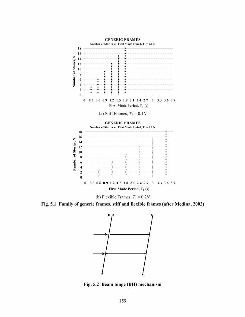
159

GENERIC FRAMES

Number of Stories vs. First Mode Period, T1 = 0.1 N

02468

1012141618

0 0.3 0.6 0.9 1.2 1.5 1.8 2.1 2.4 2.7 3 3.3 3.6 3.9First Mode Period, T1 (s)

Num

ber

of S

tori

es, N

(a) Stiff Frames, T1 = 0.1N

GENERIC FRAMESNumber of Stories vs. First Mode Period, T1 = 0.2 N

02468

1012141618

0 0.3 0.6 0.9 1.2 1.5 1.8 2.1 2.4 2.7 3 3.3 3.6 3.9First Mode Period, T1 (s)

Num

ber

of S

tori

es, N

(b) Flexible Frames, T1 = 0.2N

Fig. 5.1 Family of generic frames, stiff and flexible frames (after Medina, 2002)

Fig. 5.2 Beam hinge (BH) mechanism

160

[Sa(T1)/g]/γ vs NORM. MAX. ROOF DRIFTN=9, T1=1.8, BH, Peak Oriented Model, LMSR-N, ξ=5%,

αs=0.03, δc/δy=Var, αc=Var, γs,c,k,a=Inf, λ=0

0

2

4

6

8

10

0 1 2 3 4 5 6Norm. Max. Roof Drift, δr, max/Sd(T1) = θr,max/[Sd(T1)/H]

[Sa(T

1)/g]

/ γ

Median Non-Det. 84th Non-DetMedian Ref. System 84th Ref. System Individual Ref. System

(a) Normalized Maximum Roof Drift

[Sa(T1)/g]/γ vs NORM MAX STORY DRIFT over HEIGHTN=9, T1=1.8, BH, Peak Oriented Model, LMSR-N, ξ=5%,


0

2

4

6

8

10

0 1 2 3 4 5 6Norm Max Story Drift over Height, θs,max/[Sd(T1)/H]

[Sa(T

1)/g]

/ γ

Median Non-Det. 84th Non-DetMedian Ref. System 84th Ref. System Individual Ref. System

(b) Normalized Maximum Story Drift over Height

Fig. 5.3 Individual and statistical [Sa(T1)/g]/γ – EDP relationships for set of reference frame 0918 and statistical relationships for set of non-deteriorating frames

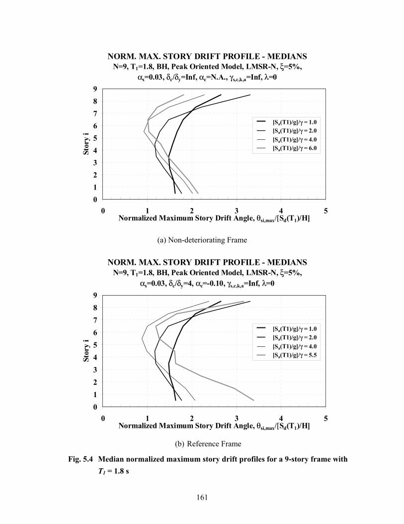
161

NORM. MAX. STORY DRIFT PROFILE - MEDIANSN=9, T1=1.8, BH, Peak Oriented Model, LMSR-N, ξ=5%,

αs=0.03, δc/δy=Inf, αc=N.A., γs,c,k,a=Inf, λ=0

0123456789

0 1 2 3 4 5Normalized Maximum Story Drift Angle, θsi,max/[Sd(T1)/H]

Stor

y i

[Sa(T1)/g]/γ = 1.0[Sa(T1)/g]/γ = 2.0[Sa(T1)/g]/γ = 4.0[Sa(T1)/g]/γ = 6.0

(a) Non-deteriorating Frame

NORM. MAX. STORY DRIFT PROFILE - MEDIANSN=9, T1=1.8, BH, Peak Oriented Model, LMSR-N, ξ=5%,

αs=0.03, δc/δy=4, αc=-0.10, γs,c,k,a=Inf, λ=0

0123456789

0 1 2 3 4 5Normalized Maximum Story Drift Angle, θsi,max/[Sd(T1)/H]

Stor

y i

[Sa(T1)/g]/γ = 1.0[Sa(T1)/g]/γ = 2.0[Sa(T1)/g]/γ = 4.0[Sa(T1)/g]/γ = 5.5

(b) Reference Frame

Fig. 5.4 Median normalized maximum story drift profiles for a 9-story frame with T1 = 1.8 s

162

EFFECT OF αc ON [Sa(T1)/g]/γN=9, T1=1.8, BH, Peak Oriented Model, LMSR-N, ξ=5%,

αs=0.03, δc/δy=4, αc=Var, γs,c,k,a=Inf, λ=0

0

2

4

6

8

10

0 4 8 12Max. of Story Drift over Story Yield Drift over the Height,

(θsi,max/θiy)max

[Sa(

T 1)/g

]/ γNon-deteriorating αc = -0.10αc = -0.30αc = -0.50

Fig. 5.5 Effect of αc of rotational springs on maximum of story drift over story

yield drift over the height, 9-story frames with T1 = 1.8 s

EFFECT OF δc/δy ON [Sa(T1)/g]/γN=9, T1=1.8, BH, Peak Oriented Model, LMSR-N, ξ=5%,

αs=0.03, δc/δy=Var, αc=-0.10, γs,c,k,a=Inf, λ=0

0

2

4

6

8

10


(θsi,max/θiy)max

[Sa(

T 1)/g

]/ γ

δc/δy = Infiniteδc/δy = 6δc/δy = 4δc/δy = 2

Fig. 5.6 Effect of δc/δy of rotational springs on maximum of story drift over story


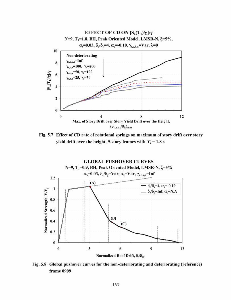
163

EFFECT OF CD ON [Sa(T1)/g]/γN=9, T1=1.8, BH, Peak Oriented Model, LMSR-N, ξ=5%,

αs=0.03, δc/δy=4, αc=-0.10, γs,c,k,a=Var, λ=0

0

2

4

6

8

10


(θsi,max/θiy)max

[Sa(

T1)

/g]/ γ


Fig. 5.7 Effect of CD rate of rotational springs on maximum of story drift over story


GLOBAL PUSHOVER CURVESN=9, T1=0.9, BH, Peak Oriented Model, LMSR-N, ξ=5%

αs=0.03, δc/δy=Var, αc=Var, γs,c,k,a=Inf

0

0.2

0.4

0.6

0.8

1

1.2

0 3 6 9 12

Normalized Roof Drift, δr/δyr

Nor

mal

ized

Str

engt

h, V

/Vy

δc/δy=4, αc=-0.10δc/δy=Inf, αc=N.A

(A)

(B)(C)

Fig. 5.8 Global pushover curves for the non-deteriorating and deteriorating (reference)

frame 0909

164

DEFLECTED SHAPE FROM PUSHOVER ANALYSIST1 = 1.8 s., N = 18, Base Case Frame Model

123456789

10111213141516171819

0 0.5 1 1.5 2 2.5 3 3.5Normalized Roof Drift, δr/δyr

Floo

r L

evel

DEFLECTED SHAPE FROM PUSHOVER ANALYSIST1 = 3.6 s., N = 18, Base Case Frame Model

123456789

10111213141516171819

0 0.5 1 1.5 2 2.5 3 3.5Normalized Roof Drift, δr/δyr

Floo

r L

evel

(a) T1 = 1.8 s. (b) T1 = 3.6 s.

Fig. 5.9 Deflected shapes from pushover analyses for non-deteriorating 18-story frames (after Medina, 2002)

DEFLECTED SHAPE FROM GLOBAL PUSHOVERN=9, T1=0.9, BH, Peak Oriented Model, LMSR-N, ξ=5%,

αs=0.03, δc/δy=Inf, αc=N.A., γs,c,k,a=Inf

1

2

3

4

5

6

7

8

9

10

0 2 4 6 8 10 12Normalized Roof Drift, δr/δyr

Floo

r Le

vel

δy/δyr = 0.60δy/δyr = 2.40δy/δyr = 4.80δy/δyr = 9.50δy/δyr = 11.7

DEFLECTED SHAPE FROM GLOBAL PUSHOVERN=9, T1=0.9, BH, Peak Oriented Model, LMSR-N, ξ=5%,

αs=0.03, δc/δy=4, αc=-0.10, γs,c,k,a=Inf

1

2

3

4

5

6

7

8

9

10

0 2 4 6 8 10 12Normalized Roof Drift, δr/δyr

Floo

r L

evel

δy/δyr = 0.60δy/δyr = 2.40δy/δyr = 4.80δy/δyr = 9.50δy/δyr = 11.7

(a) Non- Deteriorating (b) Deteriorating Reference Frame

Fig. 5.10 Deflected shapes from pushover analyses for frame 0909

165

0

10

20

30

0 0.01 0.02 0.03 0.04 0.05Rotation

Mom

ent

Roof Level

0

10

20

30

0 0.01 0.02 0.03 0.04 0.05Rotation

Mom

ent

Roof Level

0

10

20

30

0 0.01 0.02 0.03 0.04 0.05Rotation

Mom

ent

Roof Level

0

20

40

60

0 0.01 0.02 0.03 0.04 0.05Rotation

Mom

ent

Level 9

0

20

40

60

0 0.01 0.02 0.03 0.04 0.05Rotation

Mom

ent

Level 9

0

20

40

60

0 0.01 0.02 0.03 0.04 0.05Rotation

Mom

ent

Level 9

0

30

60

90

0 0.01 0.02 0.03 0.04 0.05Rotation

Mom

ent

Level 8

0

30

60

90

0 0.01 0.02 0.03 0.04 0.05Rotation

Mom

ent

Level 8

0

30

60

90

0 0.01 0.02 0.03 0.04 0.05Rotation

Mom

ent

Level 8

0

40

80

120

0 0.01 0.02 0.03 0.04 0.05Rotation

Mom

ent

Level 7

0

40

80

120

0 0.01 0.02 0.03 0.04 0.05Rotation

Mom

ent

Level 7

0

40

80

120

0 0.01 0.02 0.03 0.04 0.05Rotation

Mom

ent Level 7

0

50

100

150

0 0.01 0.02 0.03 0.04 0.05

Rotation

Mom

ent

Level 6

0

50

100

150

0 0.01 0.02 0.03 0.04 0.05

Rotation

Mom

ent

Level 6

0

50

100

150

0 0.01 0.02 0.03 0.04 0.05

RotationM

omen

t

Level 6

0

50

100

150

0 0.05 0.1 0.15

Rotation

Mom

ent

Level 5

0

50

100

150

0 0.05 0.1 0.15

Rotation

Mom

ent

Level 5

0

50

100

150

0 0.05 0.1 0.15

Rotation

Mom

ent

Level 5

0

50

100

150

0 0.05 0.1 0.15

Rotation

Mom

ent

Level 4

0

50

100

150

0 0.05 0.1 0.15

Rotation

Mom

ent

Level 4

0

50

100

150

0 0.05 0.1 0.15

Rotation

Mom

ent

Level 4

0

50

100

150

0 0.05 0.1 0.15

Rotation

Mom

ent

Level 3

0

50

100

150

0 0.05 0.1 0.15

Rotation

Mom

ent

Level 3

0

50

100

150

0 0.05 0.1 0.15

Rotation

Mom

ent

Level 3

0

50

100

150

0 0.05 0.1 0.15

Rotation

Mom

ent

Level 2

0

50

100

150

0 0.05 0.1 0.15

Rotation

Mom

ent

Level 2

0

50

100

150

0 0.05 0.1 0.15

Rotation

Mom

ent

Level 2

-90

-60

-30

0-0.15 -0.1 -0.05 0

Rotation

Mom

ent

Base-90

-60

-30

0-0.15 -0.1 -0.05 0

Rotation

Mom

ent

Base-90

-60

-30

0-0.15 -0.1 -0.05 0

Rotation

Mom

ent

Base

(a) δr/δyr = 0 to 3.1 (b) δr/δyr = 0 to 5.3 (c) δr/δyr = 0 to 6.4

Fig. 5.11 Moment–rotation relationships of rotational springs at beam ends and column base, reference frame 0909

166

0

10

20

30

Ben

ding

Mom

ent

Level 9 - Roof Level

0

10

20

30

Bend

ing

Mom

ent

Level 9 - Roof Level

0

10

20

30

Bend

ing

Mom

ent

Roof Level

0

20

40

60

Ben

ding

Mom

ent

Level 8 - Level 9

0

20

40

60

Ben

ding

Mom

ent

Level 8 - Level 9

0

20

40

60

0 3 6 9

Ben

ding

Mom

ent

Level 9

0

30

60

0 3 6 9Ben

ding

Mom

ent

Level 7 - Level 8

0

20

40

60

Ben

ding

Mom

ent

Level 7 - Level 8

0

30

60

90

Ben

ding

Mom

ent

Level 8

-100

-50

0

50

100

0 3 6 9

Ben

ding

Mom

ent

Level 6 - Level 7

0

50

100

150B

endi

ng M

omen

t

Level 6 - Level 7

0

50

100

150

Ben

ding

Mom

ent

Level 7

-150

-100

-50

0

50

100

0 3 6 9

Ben

ding

Mom

ent

Level 5 - Level 6

0

50

100

150

200

Ben

ding

Mom

ent

Level 5 - Level 6

0

50

100

150

Ben

ding

Mom

ent

Level 6

-150

-100

-50

0

50

100

0 3 6 9

Ben

ding

Mom

ent

Level 4 - Level 5

0

50

100

150

200

Ben

ding

Mom

ent

Level 4 - Level 5

0

50

100

150B

endi

ng M

omen

tLevel 5

-100

-50

0

50

100

0 3 6 9

Ben

ding

Mom

ent

Level 3 - Level 4

0

50

100

150

200

Ben

ding

Mom

ent

Level 3 - Level 4

0

50

100

150

Ben

ding

Mom

ent

Level 4

-50

0

50

100

0 3 6 9

Ben

ding

Mom

ent

Level 2 - Level 3

0

50

100

150

Ben

ding

Mom

ent

Level 2 - Level 3

0

50

100

150

Ben

ding

Mom

ent

Level 3

0

30

60

90

Ben

ding

Mom

ent

Base - Level 2

0

30

60

90

Ben

ding

Mom

ent

Base - Level 2

0

50

100

150

0 3 6 9

Ben

ding

Mom

ent

Level 2

(a) Column, Lower Level (b) Column, Upper Level (c) Beam

Fig. 5.12 Moment (*1/1000) vs. normalized roof drift of columns and beams of reference frame 0909

167

Sa(T1)/g vs MAX. ROOF DRIFT ANGLE, γ=0.6N=3, T1=0.3, BH, Peak Oriented Model, LMSR-N, ξ=5%,


0

1

2

3

4

5

6

0 0.005 0.01 0.015 0.02Maximum Roof Drift Angle, θr,max = δr,max/H

S a(T

1)/g

Median84thIndividualGlobal Pushover

Sa(T1)/g vs MAX. ROOF DRIFT ANGLE, γ=0.6N=3, T1=0.6, BH, Peak Oriented Model, LMSR-N, ξ=5%,


0

2

4

6

8

0 0.02 0.04 0.06Maximum Roof Drift Angle, θr,max = δr,max/H

S a(T

1)/g


(a) Frame 0303, γ = 0.6 (b) Frame 0306, γ = 0.6

Fig. 5.13 Maximum roof drift angle from dynamic and static nonlinear analysis for the 3-story reference frames

Sa(T1)/g vs MAXIMUM ROOF DRIFT ANGLE, γ=0.4N=9, T1=0.9, BH, Peak Oriented Model, LMSR-N, ξ=5%,


0

1

2

3

4

5

0 0.01 0.02 0.03 0.04Maximum Roof Drift Angle, θr,max=δr,max/H

S a(T

1)/g


Sa(T1)/g vs MAXIMUM ROOF DRIFT ANGLE, γ=0.2N=9, T1=1.8, BH, Peak Oriented Model, LMSR-N, ξ=5%,


0

0.5

1

1.5

2

0 0.02 0.04 0.06Maximum Roof Drift Angle, θr,max=δr,max/H

S a(T

1)/g


(a) Frame 0909, γ = 0.4 (b) Frame 0918, γ = 0.2

Fig. 5.14 Maximum roof drift angle from dynamic and static nonlinear analysis for the 9-story reference frames

θs,max/θr,max MEDIAN RATIOS vs Sa(T1)/g, γ=Var

N=Var, T1=Var, BH, Peak Oriented Model, LMSR-N, ξ=5%, αs=0.03, δc/δy=4, αc=-0.10, γs,c,k,a=Inf, λ=0

0

1

2

3

4

0 1 2 3 4 5 6Median θs,max/θr,max Ratios

S a(T

1)/g

030303060909091818181836

Fig. 5.15 Ratio of maximum interstory drift angle over maximum roof drift angle, 3

and 9-story-reference frames

168

MEDIAN and 16th [Sa,c(T1)/g]/γ vs PERIODN=Var, T1=Var, BH, Peak Oriented Model, LMSR-N, ξ=5%,


0

2

4

6

8

10

0 1 2 3 4Fundamental Period, T1 (sec)

[Sa,

c(T1)

/g]/ γ

0303

1515

121209090606

1818

03060612

1224

0918

1836

1530

Median, T1 = 0.1N16th, T1 = 0.1NMedian, T1 = 0.2N16th, T1 = 0.2N

Fig. 5.16 Median and 16th percentile collapse capacity spectra, set of reference

frames

MEDIAN [Sa,c(T1)/g]/γ vs PERIODN=Var, T1=Var, BH, Peak Oriented Model, LMSR-N, ξ=5%,


0

2

4

6

8

10

0 5 10 15 20Number of Stories

[Sa,

c(T1)

/g]/ γ

0303

1515

121209090606

1818

0306 0612

1224

0918

1836

1530

T1 = 0.1NT1 = 0.2N

Fig. 5.17 Median collapse capacities — number of stories, set of reference frames

169

POST-CAPPING STIFFNESS EFFECT ON [Sa,c(T1)/g]/γ N=Var, T1=Var, BH, Peak Oriented Model, LMSR-N, ξ=5%,


0

2

4

6

8

10


[Sa,

c(T1)/

g]/ γ

αc = -0.1αc = -0.3αc = -0.5

T1 = 0.1 NT1 = 0.2 N

(a) Median Collapse Capacity Spectra

POST-CAPPING STIFFNESS EFFECT ON [Sa,c(T1)/g]/γ

N=Var, T1=Var, BH, Peak Oriented Model, LMSR-N, ξ=5%, αs=0.03, δc/δy=4, αc=Var, γs,c,k,a=Inf, λ=0

0

0.2

0.4

0.6

0.8

1

1.2


Var

iatio

n / B

ase

Cas

e

αc = -0.1αc = -0.3αc = -0.5

T1 = 0.1 NT1 = 0.2 N

DISPERSION OF [Sa,c(T1)/g]/γ N=Var, T1=Var, BH, Peak Oriented Model, LMSR-N, ξ=5%,


0

0.2

0.4

0.6

0.8

1


Stan

dard

Dev

. ln[

S a,c(

T1)/

g]/ γ αc = -0.1

αc = -0.3αc = -0.5

T1 = 0.1 NT1 = 0.2 N

(b) Median Ratios of Col. Capacity Spectra (c) Dispersion of Collapse Capacity Spectra Fig. 5.18 Effect of αc of springs on collapse capacity of generic frames, δc/δy = 4, γs,c,k,a = inf.

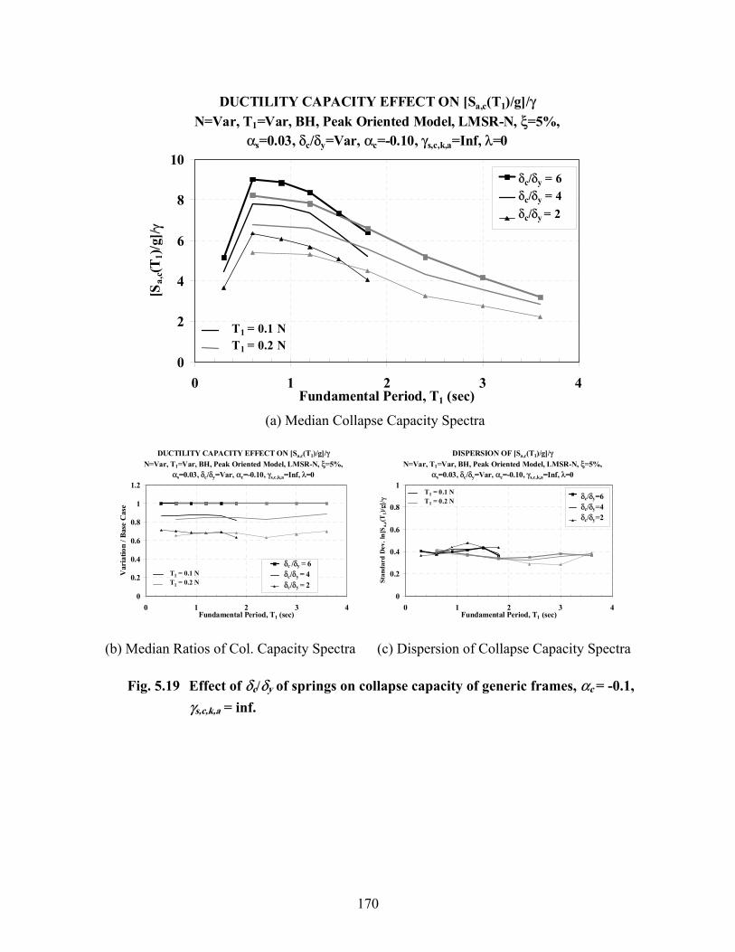
170

DUCTILITY CAPACITY EFFECT ON [Sa,c(T1)/g]/γ N=Var, T1=Var, BH, Peak Oriented Model, LMSR-N, ξ=5%,


0

2

4

6

8

10


[Sa,

c(T1)/

g]/ γ

δc/δy = 6 δc/δy = 4δc/δy = 2

T1 = 0.1 NT1 = 0.2 N


DUCTILITY CAPACITY EFFECT ON [Sa,c(T1)/g]/γ

N=Var, T1=Var, BH, Peak Oriented Model, LMSR-N, ξ=5%, αs=0.03, δc/δy=Var, αc=-0.10, γs,c,k,a=Inf, λ=0

0

0.2

0.4

0.6

0.8

1

1.2


Var

iatio

n / B

ase

Cas

e

δc /δy = 6δc/δy = 4δc/δy = 2

T1 = 0.1 NT1 = 0.2 N



0

0.2

0.4

0.6

0.8

1


Stan

dard

Dev

. ln[

S a,c(

T1)/

g]/ γ δc/δy=6

δc/δy=4δc/δy=2

T1 = 0.1 NT1 = 0.2 N

(b) Median Ratios of Col. Capacity Spectra (c) Dispersion of Collapse Capacity Spectra

Fig. 5.19 Effect of δc/δy of springs on collapse capacity of generic frames, αc = -0.1, γs,c,k,a = inf.

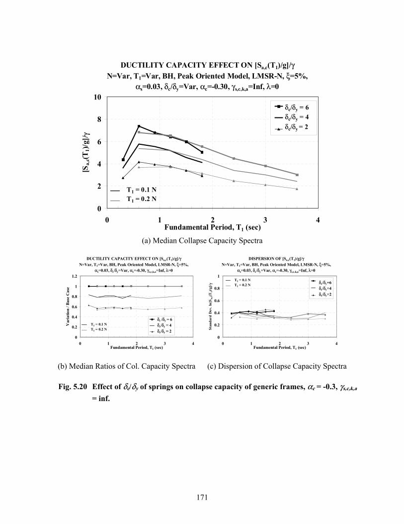
171



0

2

4

6

8

10


[Sa,

c(T1)/

g]/ γ

δc/δy = 6 δc/δy = 4δc/δy = 2

T1 = 0.1 NT1 = 0.2 N




0

0.2

0.4

0.6

0.8

1

1.2


Var

iatio

n / B

ase

Cas

e

δc /δy = 6δc/δy = 4δc/δy = 2

T1 = 0.1 NT1 = 0.2 N



0

0.2

0.4

0.6

0.8

1


Stan

dard

Dev

. ln[

S a,c(

T1)/

g]/ γ δc/δy=6

δc/δy=4δc/δy=2

T1 = 0.1 NT1 = 0.2 N

(b) Median Ratios of Col. Capacity Spectra (c) Dispersion of Collapse Capacity Spectra

Fig. 5.20 Effect of δc/δy of springs on collapse capacity of generic frames, αc = -0.3, γs,c,k,a

= inf.

172

CYCLIC DETERIORATION EFFECT ON [Sa,c(T1)/g]/γ N=Var, T1=Var, BH, Peak Oriented Model, LMSR-N, ξ=5%,


0

2

4

6

8

10


[Sa,

c(T1)/

g]/ γ

γs,c,k,a= Infγs,c,k,a=100γs,c,k,a=50γs,c,k,a=25

T1 = 0.1 NT1 = 0.2 N


CYCLIC DETERIORATION EFFECT ON [Sa,c(T1)/g]/γ

N=Var, T1=Var, BH, Peak Oriented Model, LMSR-N, ξ=5%, αs=0.03, δc/δy=4, αc=-0.10, γs,c,k,a=Var, λ=0

0

0.2

0.4

0.6

0.8

1

1.2


Var

iatio

n / B

ase

Cas

e

γs,c,k,a=Inf γs,c,k,a=100γs,c,k,a=50 γs,c,k,a=25



0

0.2

0.4

0.6


Stan

dard

Dev

. ln[

S a,c(

T1)/

g]/ γ

γs,c,k,a= Infγs,c,k,a=100γs,c,k,a=50γs,c,k,a=25T1 = 0.1 N

T1 = 0.2 N

(b) Median Ratios of Col. Capacity Spectra (c) Dispersion of Collapse Capacity Spectra Fig. 5.21 Effect of CD of springs on collapse capacity of generic frames, δc/δy = 4, αc = -0.1

173

HYSTERETIC MODEL EFFECT ON [Sa,c(T1)/g]/γ N=Var, T1=Var, BH, LMSR-N, ξ=5%,

αs=0.03, δc/δy=Var, αcap=-0.10, γs,c,k,a=Inf, λ=0

0

2

4

6

8

10


[Sa,

c(T1)

/g]/ γ

Pinching, T = 0.1NPinching, T=0.2NPeak Oriented, T=0.1NPeak Oriented, T=0.2NBilinear, T=0.1NBilinear, T=0.2N

Fig. 5.22 Effect of hysteretic model on median collapse capacity of generic frames

GLOBAL PUSHOVER CURVESN=18, T1=3.6, BH, Peak Oriented Model, LMSR-N, ξ=5%,

αs=0.03, δc/δy=Inf, αc=N.A, γs,c,k,a=Inf, λ=0

0

0.2

0.4

0.6

0.8

1

1.2

0 0.5 1 1.5 2 2.5 3Normalized Roof Displacement, δr/δyr

Nor

mal

ized

Str

engt

h, V

/Vy

θe=0.09

θi=0.37

Pushover Curve with P-∆ EffectsPushover Curve w/o P-∆ Effects

αs,0K0=0.04K0

Κ0

Fig. 5.23 Elastic and inelastic stability coefficients obtained from global pushover

curves, peak oriented non-deteriorating frame 1836

174

GLOBAL STABILITY COEFFICIENTT1=0.1N &T1=0.2N

0%

5%

10%

15%

20%

25%

30%

35%

40%

0 3 6 9 12 15 18 21Number of Stories (N)

Glo

bal S

tabi

lity

Coe

ffic

ient

θe, T1 = 0.1Nθi, Τ1 = 0.1Νθe, Τ1 = 0.2Νθi, Τ1 = 0.2Ν

(a) Stability Coefficients from Global Pushover Curves

POST-YIELD STIFFNESS RATIO OF GLOBAL

PUSHOVER CURVE

-0.35

-0.3

-0.25

-0.2

-0.15

-0.1

-0.05

0

0.05

0.1

0 3 6 9 12 15 18 21Number of Stories (N)

Post

-Yie

ld S

tiffn

ess R

atio

of

Push

over

Cur

ve

P-∆ = 0P - ∆ = 0.1NP - ∆ = 0.2N

P-∆ = 0P - ∆ = 0.1NP - ∆ = 0.2N

(c) Post-Yield Stiffness Ratio in Global Pushover Curve

Fig. 5.24 Post-yield stiffness ratio and stability coefficients from global pushover curves, generic frames with strain hardening in rotational springs of 3%

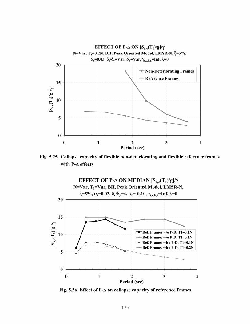
175

EFFECT OF P-∆ ON [Sa,c(T1)/g]/γN=Var, T1=0.2N, BH, Peak Oriented Model, LMSR-N, ξ=5%,


0

5

10

15

20


[Sa,

c(T1)

/g]/ γ

Non-Deteriorating Frames

Reference Frames

Fig. 5.25 Collapse capacity of flexible non-deteriorating and flexible reference frames

with P-∆ effects

EFFECT OF P-∆ ON MEDIAN [Sa,c(T1)/g]/γN=Var, T1=Var, BH, Peak Oriented Model, LMSR-N,

ξ=5%, αs=0.03, δc/δy=4, αc=-0.10, γs,c,k,a=Inf, λ=0

0

5

10

15

20


[Sa,

c(T1)

/g]/ γ

Ref. Frames w/o P-D, T1=0.1NRef. Frames w/o P-D, T1=0.2NRef. Frames with P-D, T1=0.1NRef. Frames with P-D, T1=0.2N

Fig. 5.26 Effect of P-∆ on collapse capacity of reference frames

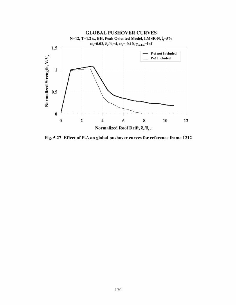
176

GLOBAL PUSHOVER CURVESN=12, T=1.2 s., BH, Peak Oriented Model, LMSR-N, ξ=5%

αs=0.03, δc/δy=4, αc=-0.10, γs,c,k,a=Inf

0

0.5

1

1.5

0 2 4 6 8 10 12Normalized Roof Drift, δr/δy,r

Nor

mal

ized

Str

engt

h, V

/Vy P-∆ not Included

P-∆ Included

Fig. 5.27 Effect of P-∆ on global pushover curves for reference frame 1212

177

MAX. STRONG COLUMN FACTOR OVER HEIGHTN=9, T1=0.9, BH, Peak Oriented Model, LMSR-N, ξ=5%,

θe=0.015, αs=0.03, δc/δy=4, αc=-0.10, γs,c,k,a=Inf, λ=0

0

2

4

6

8

10

12

14

16

0 1 2 3 4 5 6Maximum Strong Column Factor Over Height (2Mc/Mp,b)

[Sa(

T1)

/g]/ γ

Median84thIndividual

Fig. 5.28 Maximum strong-column factor over the height for reference frame 0909

MEDIAN [Sa,c(T1)/g]/γ vs PERIODN=Var, T1=Var, BH & BH-CH, P. O. Model, LMSR-N,


0

2

4

6

8

10


[Sa,

c(T1)

/g]/ γ

BH-CH, T1 = 0.1NBH-CH, T1 = 0.2NBH, T1 = 0.1NBH, T1 = 0.2N

ΣMc = 2.4Mb,p

Fig. 5.29 Effect on median collapse capacity of including columns with high strength

( pbc MM ,4.2∑ = )

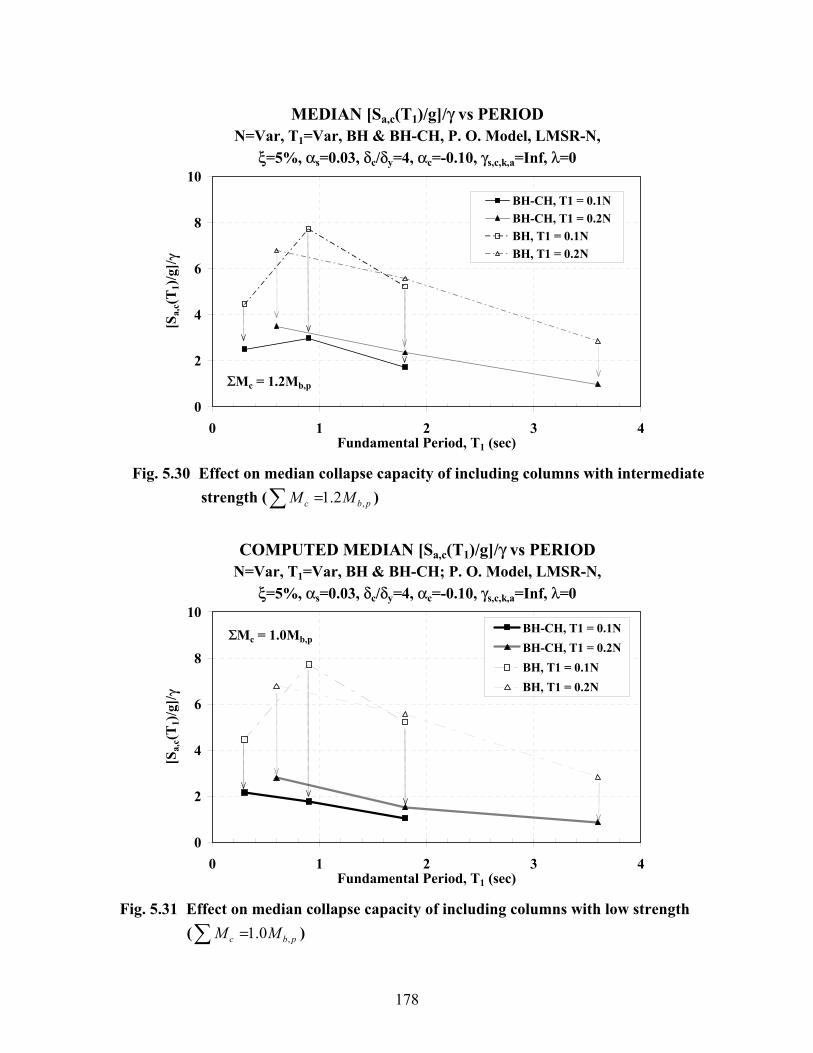
178

MEDIAN [Sa,c(T1)/g]/γ vs PERIODN=Var, T1=Var, BH & BH-CH, P. O. Model, LMSR-N,


0

2

4

6

8

10


[Sa,

c(T1)

/g]/ γ


ΣMc = 1.2Mb,p

Fig. 5.30 Effect on median collapse capacity of including columns with intermediate

strength ( pbc MM ,2.1∑ = )

COMPUTED MEDIAN [Sa,c(T1)/g]/γ vs PERIODN=Var, T1=Var, BH & BH-CH; P. O. Model, LMSR-N,


0

2

4

6

8

10


[Sa,

c(T1)

/g]/ γ


ΣMc = 1.0Mb,p

Fig. 5.31 Effect on median collapse capacity of including columns with low strength

( pbc MM ,0.1∑ = )

179

(a) P-∆ Representation by Rotation of Hysteresis Diagram

(b) Incorrect P-∆ Representation by Adjustment of Post-Yield Stiffness

Fig. 5.32 Representation of P-∆ effects in SDOF systems

Ke

Fy+ F

0

Fy-

Loading Path with P-∆ Effects

θKe

(αs-θ)Ke

αsKe

(1-θ)Fy+

Backbone Curve without P-∆ Effects

δy

(1-θ)Ke

Loading Path w/incorrect P-∆ Representation

Ke

Fy+

δ

F

0

Fy-

θKe

αsKe

Backbone Curve without P-∆ Effects

δy

180

Fig. 5.33 P-∆ Effects obtained with an auxiliary backbone curve based on elastic and inelastic stability coefficients

Fig. 5.34 P-∆ Effects obtained with a simplified auxiliary backbone curve and rotation

of the strain hardening branch by the inelastic stability coefficient

θauxKaux

Kaux

αs,0K0 Fy,0

Fy,aux αs,auxKaux

Auxiliary Backbone Curve

θauxKaux

(αs,0-θi)K0

δy

θeK0

F

δ

K0 Fy,P∆

KP∆

θauxKaux

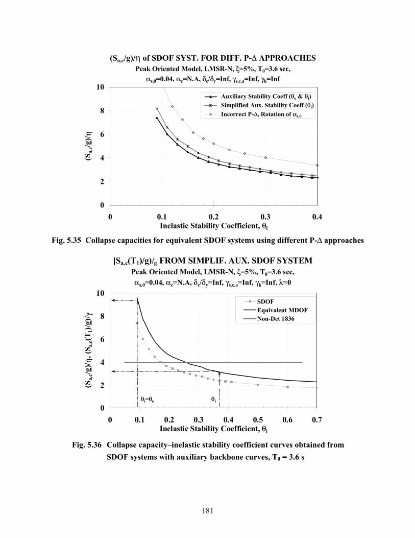
181

(Sa,c/g)/η of SDOF SYST. FOR DIFF. P-∆ APPROACHESPeak Oriented Model, LMSR-N, ξ=5%, T0=3.6 sec,

αs,0=0.04, αc=N.A, δc/δy=Inf, γs,c,a=Inf, γk=Inf

0

2

4

6

8

10

0 0.1 0.2 0.3 0.4Inelastic Stability Coefficient, θi

(Sa,

c/g)/ η

Auxiliary Stability Coeff (θe & θi)Simplified Aux. Stability Coeff (θi)Incorrect P-∆, Rotation of αs,0

Fig. 5.35 Collapse capacities for equivalent SDOF systems using different P-∆ approaches

[Sa,c(T1)/g)/g FROM SIMPLIF. AUX. SDOF SYSTEMPeak Oriented Model, LMSR-N, ξ=5%, T0=3.6 sec, αs,0=0.04, αc=N.A, δc/δy=Inf, γs,c,a=Inf, γk=Inf, λ=0

0

2

4

6

8

10

0 0.1 0.2 0.3 0.4 0.5 0.6 0.7Inelastic Stability Coefficient, θi

(Sa,

c/g)/ η

, (S a

,c(T

1)/g

)/ γ

SDOFEquivalent MDOFNon-Det 1836

θi=θe θi

Fig. 5.36 Collapse capacity–inelastic stability coefficient curves obtained from

SDOF systems with auxiliary backbone curves, T0 = 3.6 s

182

[Sa,c(T1)/g]/γ FROM SIMPLIF. AUX. SDOF SYSTEMPeak Oriented Model, LMSR-N, ξ=5%, T0=3.6 sec,


0

2

4

6

8

10

0 0.1 0.2 0.3 0.4 0.5 0.6 0.7Stability Coefficient, θi

(Sa,

c(T)/g

)/ η, [

S a,c(T

1)/g

]/ γ

SDOFEquivalent MDOFNon-Det. 1836, Strain Hard=0% Non-Det. 1836, Strain Hard=3% Non-Det. 1836, Strain Hard=6%

Fig. 5.37 Test of collapse capacity–inelastic stability coefficient curves for MDOF

structures with T0 = 3.6 s. and variations of αs at the rotational springs

[Sa,c(T1)/g)/γ FROM SIMPLIF. AUX. SDOF SYSTEMPeak Oriented Model, LMSR-N, ξ=5%, T0=3.6 sec,


0

2

4

6

8

10

0 0.1 0.2 0.3 0.4 0.5 0.6 0.7Stability Coefficient, θi

(Sa,

c(T)/g

)/ η, [

S a,c(T

1)]/g

)/ γ

SDOFEquivalent MDOFNon-Det. 1836, P/W = 1.4Non-Det. 1836, P/W = 1.2Non-Det. 1836, P/W = 1.0

Fig. 5.38 Test of collapse capacity–inelastic stability coefficient curves for MDOF structures with T0 = 3.6 s. and variations of P/W ratio

6 Effect of Uncertainty in System Parameters on the Variance of Collapse Capacity

6.1 INTRODUCTION

In previous chapters, collapse capacity has been evaluated considering deterministic system

parameters, and record to record (RTR) variability has been the only source of uncertainty

included in the dispersion of collapse capacity. Although the parameters of the structural system

are also subjected to uncertainty, small attention has been paid to the study of probability

distributions of system parameters. The main assumption has been that uncertainties related to

the system parameters are expected to be small compared to those originated by RTR variability.

For instance, Esteva and Ruiz (1989) studied the probability of failure of reinforced concrete

(RC) MDOF structures when uncertainty is included in the system parameters. They utilized

non-deteriorating systems and considered failure when the ductility demand at any given story

reached some predetermined available capacity. Statistical information for parameters such as

yielding strength of the bars, concrete strength, and dimensions was taken from investigations on

distributions of the system parameters carried out by Mirza and McGregor (1979)16. The

conclusion was that uncertainty of the aforementioned parameters did not produce large

modifications on the probability of failure of the system.

The small effect of uncertainty in the system parameters on the response of non-

deteriorating systems has led to the practice of replacing the distributions of the parameters with

expected values. However, the uncertainty of system parameters in deteriorating systems has not

been systematically evaluated. The results of chapters 4 and 5 suggest that the variance of

collapse capacity could be significantly influenced by uncertainty in parameters that define the

hysteresis model, such as ductility capacity, post-capping, stiffness or CD rate. The level of

16 First moments and distributions of system parameters also can be found in Ellingwood (1983).

184

uncertainty of these parameters is large because of the intrinsic large aleatory variability in the

nonlinear range and the inability to accurately evaluate these parameters, i.e., the epistemic

uncertainty is also large.

In this chapter, the sensitivity of collapse capacity to uncertainty in the system

parameters is investigated by using the first-order second-moment method (FOSM), whereas

Monte Carlo simulations are employed to verify the accuracy of FOSM results. In the first part,

different alternatives for applying the FOSM method to collapse capacity evaluation are explored

for an SDOF system of intermediate ductile characteristics. Thereafter, the increment in the

variance of collapse capacity is obtained for representative SDOF systems and for a set of

generic frames with intermediate ductile features.

1.1 6.2 FOSM METHOD

6.2.1 General Formulation

Given a function Y = f(Q1, Q2,…, Qn) and given that Q is a random vector, the mean and

variance of Y can be approximated by a Taylor’s series expansion of the performance function (f)

about the expected values of the random variables (Wolff, 1994; Melchers, 1999; Baker and

Cornell, 2003). The simplest approximation is termed a first-order second-moment (FOSM)

method, as only first-order (linear) terms of the series are retained and only the first two

moments (mean and variance) are considered. This means that the method is exact for linear

performance functions, and that for a given degree of curvature, the method is more accurate for

smaller values of the variances. The first two moments are calculated as follows:

)(),...,,(21 QQQQY ff

nµµµµµ =≅ (6.1)

∑∑= = =

⎟⎟⎠

⎞⎜⎜⎝

⎛

∂∂

∂∂≅

n

i

n

jqqqq

QjiY jiji

qqQf

qQf

1 1,

2 )()( σσρσµ

(6.2)

where Q is the vector of random system parameters, qµ is the vector of mean values of Q , and

the correlation coefficient is equal to:

ji qq

jiji

QQCovσσ

ρ)(

, = (6.3)

185

Note that the first moments of Y can be estimated without knowing the probability

distribution of the function Y = f(Q ). The relative magnitudes of the terms in Equation 6.2

provide an explicit indication of the contribution to uncertainty of each variable. The

disadvantages of the method are that it is necessary to approximate the value of the derivatives

and that an error for nonlinear functions can be introduced by neglecting higher-order terms.

In the application of the method for computing the variance of collapse capacity, an

additional term needs to be added to Equation 6.2 to account for the already calculated RTR

variability (Section 6.2.2). Also, because FOSM is a simplified method that requires little

information to be implemented, several alternatives for approximating the derivative of the

function “f” in Equation 6.2 are presented in Section 6.2.3.

6.2.2 Computations in Log Domain of Data

In last section, the FOSM formulation is expressed in the linear domain of the data, i.e., the

parameter values and collapse capacities utilized in Equations 6.1–6.3 are obtained directly from

the time history analyses (THA). However, in this research it is preferred to compute the

additional variance of collapse capacity in the log domain of the data, i.e., by using the natural

logarithm of the parameter values and corresponding collapse capacities. The main reason is that

high nonlinearities in the system parameters – collapse capacity relationships tend to be reduced

in the log domain. Therefore, the results become less sensitive to numerical variations because

the likelihood of evaluating collapse capacity in a highly nonlinear region is reduced. Appendix

D provides more details of the reasons for preferring the computations in the log domain of the

data.

The following formulation is derived from the methodology proposed by Baker and

Cornell (2003) for estimating the role of supplementary variables in uncertainty. To compute the

total variance in the log domain, collapse capacity 17 is initially expressed in the linear domain

as:

17 Collapse capacity was defined in Chapter 2 as [(Sa/g)/η]c for SDOF systems and as {[(Sa(T1)/g)]/γ}c for MDOF systems. For the sake of simplicity, in this chapter this nomenclature is usually shortened to Sa,c/η for SDOF systems and to Sa,c(T1)/γ for MDOF structures (although for developing the formulation, only Sa,c/η is used). If collapse capacity is used as a subscript, the nomenclature is simplified to Sa,c.

186

( )RTRQQQfS knca εη ).,...,,(/ 21, = (6.4)

where the random variable ( )RTRkε has a mean equal to one. This formulation is called the

“multiplicative approach” because in the linear domain ( )RTRkε is a multiplier to the function

),...,,( 21 nQQQf . Taking the natural log on both sides of Equation 6.4:

))(ln()),...,,ln()/ln( 21, RTRQQQS knca εη += (6.5)

Observe that in the log domain )](ln[ RTRkε is added to the new function “g.” By using

QX ln= , Equation 6.5 becomes:

))(ln()),...,,()/ln( 21, RTRXXXgS knca εη += (6.6)

Since the expected value of )](ln[ RTRkε is equal to zero, the FOSM method estimates the mean

as:

)(ln , XgS caµµ ≅ (6.7)

The variance of )](ln[ RTRkε is equal to 2)(ln , RTRS ca

σ , which is the variance of the collapse

capacity when the system parameters are deterministic and the only source of uncertainty is RTR

variability. Thus, the first-order approximation of the variance of collapse capacity is 18:

2)(ln

1 1,

2)(ln ,,

)()(RTRS

n

i

n

jxxxx

XjiTOTS cajiji

x

ca xXg

xXg σσσρσ

µ

+⎟⎟⎠

⎞⎜⎜⎝

⎛

∂∂

∂∂≅∑∑

= = =

(6.8)

The first term on the right-hand side of Equation 6.8 represents the contribution to the

variance of collapse capacity due to uncertainty of all the system parameters. The correlation

coefficient, ji xx ,ρ , is calculated in the same way as

ji qq ,ρ (Equation 6.3).

If only one probabilistic system parameter is involved, Equation 6.8 simplifies to:

2)(ln

22

2)(ln ,,

)(RTRSx

xTOTS caca x

g σσµσ +⎟⎠⎞

⎜⎝⎛

∂∂≅ (6.9)

Note that in the log domain of the data, the variance of collapse capacity due to RTR

variability ( 2)(ln , RTRS ca

σ ) is added to the variance of collapse capacity due to uncertainty in the

18 The term 2)(, TOTS ca

σ is denoted as Var[Sa,c(TOT)] in the graphs of this chapter.

187

system parameters. This formulation assumes that, in the linear domain, the coefficient of

variation of collapse capacity due to RTR variability is a constant for variations of the

probabilistic parameter, i.e., )(,... RTRS ca

voc is constant under variations of xi (see Appendix D).

6.2.3 Computation of Derivative

An approximation of the derivate, iX xg ∆∆ /)(µ , needed to evaluate Equation 6.8 may be

obtained in several ways. For instance, the performance function may be evaluated at two system

parameter values and the derivative estimated as the slope of the straight line that connects the

pairs [xi, g(xi)]. The simplest option is to consider the mean of the system parameter and its

corresponding collapse capacity as one pair because these values are known. The second point

can be any increment above or below the mean. It is recommended to take the increment as one

standard deviation to capture some of the nonlinear behavior of the function over a range of

likely values (Wolff, 1994; Baker and Cornell, 2003). In Figure 6.1, the straight line connecting

these two points is dubbed “secant 1,” and from now on, this approach will be referred as the

“one-side” approach. The increment with respect to the mean value is represented as σn±=∆ ,

where n is a multiplier. For computations in the log domain of the data:

x

xxxSxxSx

nnxx

xg acac

σσµµµµµ

±±=−=

≅∂

∂ )()()( 2)(ln1)(ln 21 (6.10)

where )()(ln ixS xiac

µ is the log of the estimator of the geometric mean of collapse capacity (due to

RTR variability) when the probabilistic system parameters are )exp( 1x and )exp( 2x 19. This is an

additional approximation because the estimator of the geometric mean is modified according to

the GMs included in the bin. After this simplification the only source of uncertainty in the

computation of the derivative is the uncertainty in the probabilistic parameter.

A second alternative to compute the derivative is to select the points located at one

increment above and below the expected value of the random system parameter (Wolff, 1994).

This option, which is referred as the “two-side” approach, is shown in Figure 6.1 with the

straight line dubbed “secant 2.” For smooth functions this method should result in a better

19 Remember that QX ln= .

188

approximation because the slope of “secant 2” is closer to the derivative evaluated at xµ . The

computational effort increases because collapse capacity needs to be evaluated at two additional

system parameter values. For computations in the log domain of the data, the derivative is

approximated as:

x

xxxSxxxSx

nnxnx

xg acac

σσµµσµµµ

2)()()( 2)(ln1)(ln 21

±−=−+=

≅∂

∂ (6.11)

There are other approaches for calculating the derivative such as the standard numerical

differentiation method, which utilizes a central difference representation for the derivative

(Hornbeck, 1975). These methods are not implemented because they involve a larger

computational effort and a pilot study did not improve the accuracy of the results.

6.2.4 FOSM Equation for Parameter Study

In subsequent sections, δc/δy, αc and γs,c,k,a are considered the probabilistic system parameters of

the structural system. For the sake of simplicity, the nomenclature of these parameters is

shortened to δ, α, and γ, respectively, and Equation 6.8 can be particularized as follows:

2)(lnlnln

lnln

lnln

2ln

22ln

22ln

22ln

,

lnlnln

lnlnln

lnlnln

lnlnln

lnlnln

lnlnln,

),,(),,(2

),,(),,(2

),,(),,(2

),,(),,(),,(

RTRS

S

ca

ca

gg

gg

gg

ggg

σσσργ

γαδα

γαδ

σσργ

γαδδ

γαδ

σσρα

γαδδ

γαδ

σγ

γαδσα

γαδσδ

γαδσ

γααγ

µγµαµδ

γδδγ

µγµαµδ

αδαδ

µγµαµδ

γ

µγµαµδα

µγµαµδδ

µγµαµδ

γαδ

γαδ

γαδ

γαδ

γαδ

γαδ

+⎟⎟⎠

⎞⎜⎜⎝

⎛∂

∂⎟⎠⎞

⎜⎝⎛

∂∂

+⎟⎟⎠

⎞⎜⎜⎝

⎛∂

∂⎟⎠⎞

⎜⎝⎛

∂∂

+⎟⎠⎞

⎜⎝⎛

∂∂

⎟⎠⎞

⎜⎝⎛

∂∂

+⎟⎟⎠

⎞⎜⎜⎝

⎛∂

∂+⎟⎠⎞

⎜⎝⎛

∂∂+⎟

⎠⎞

⎜⎝⎛

∂∂=

===

===

===

===

===

===

(6.12)

In this shortened nomenclature, for instance, the term γαδ

µγµαµδδ

γαδ

lnlnln

2),,(

===⎟

⎠⎞

⎜⎝⎛

∂∂g refers to the

square of the derivative of the function “g” with respect to the system parameter δc/δy. The

189

function “g” depends on the parameters δc/δy, αc, and γs,c,k,a. The derivative is obtained around

the mean values of each one of the probabilistic parameters.

The first three terms of Equation 6.12 correspond to contributions to the variance of the

natural logarithm of collapse capacity due to uncertainty in δc/δy, αc, and γs,c,k,a. The following

three terms involve correlations among these three parameters. For example, the fourth term is

dubbed “δα correlation” and expresses the dependence of one parameter on the other one. In the

following sections, the terms for the contributions to total variance of the log of collapse capacity

are shortened as follows:

2)(ln

2)(ln

2)(ln

2)(ln

2)(ln

2)(ln

2)(ln

2)(ln

,.,.,.,

,,,,

RTRSSSS

SSSTOTS

cacacaca

cacacaca

σσσσ

σσσσ

γαγδδα ρρρ

γδα

+++

+++= (6.13)

2)(ln , ασ

caS is the contribution to variance of the log of collapse capacity due to uncertainty

in post-capping stiffness. Similar interpretation is given to 2)(ln , δσ

caS and 2)(ln , γσ

caS .

2)(ln ., αδρσ

caS is the contribution to variance of the log of collapse capacity due to correlation

between the parameters δ and α. Similar explanation is given to the terms 2)(ln ., γδρσ

caS and

2)(ln ., γαρσ

caS .

The three terms involving correlation among parameters can be condensed into a term

called “combined correlation.” Therefore, Equation 6.13 is condensed to:

2

)(ln2

)(ln2

)(ln2

)(ln2

)(ln2

)(ln ,,,,,, RTRSSSSSTOTS caTcacacacacaσσσσσσ ργδα ++++= (6.14)

where 2)(ln

2)(ln

2)(ln

2)(ln .,.,.,, γαγδδα ρρρρ σσσσ

cacacaTca SSSS ++= .

Sometimes all the contributions to variance of the log of collapse capacity due to the

system parameters are grouped into a single term, 2)(ln , XS ca

σ , and Equation 6.14 is simplified as

follows: 2

)(ln2

)(ln2

)(ln ,,, RTRSXSTOTS cacacaσσσ += (6.15)

190

6.3 EVALUATION OF FOSM METHOD FOR OBTAINING VARIANCE OF COLLAPSE CAPACITY

This section explores the most suitable alternatives for computing additional variance of collapse

capacity using the FOSM method. Because the method is an approximation that simplifies the

nature of the problem, the validity of obtained results depends on the assumptions made for each

particular situation. For this reason, this section is divided into three parts. In the first part, only

one system parameter at a time is considered in a probabilistic format. At this point, the most

consistent alternatives for applying the FOSM method to a single probabilistic parameter are

selected. In a second stage, uncertainty of several parameters is considered at the same time to

evaluate the effect of correlation among them. In the third part, Monte Carlo simulation is used

for verifying some of the results obtained by the FOSM method.

The SDOF system used for these evaluations is the reference system of Chapter 4, which

is subjected to the set of records LMSR-N and has the following features:

• Peak-oriented hysteretic model

• No P-∆ effect

• Medium ductility capacity, δc/δy = 4

• Small post-capping stiffness, αc = -0.1 Ke

• Slow cyclic deterioration rate, γs,c,k,a = 100

Variance of System Parameters. Statistical information about the parameters that define

the hysteretic backbone and its corresponding cyclic deterioration are difficult to find in the

literature. Possibly the best source for RC components is the database collected by Fardis and

Biskinis (2003), in which statistical information for yield and ultimate rotation of components

with different characteristics is presented. The ultimate rotation is defined as the rotation at

which 15% of the peak strength is lost. The coefficients of variation (c.o.v.) of the yield and

ultimate rotation is used for estimating the standard deviation of the log of ductility capacity in

an approximated way because the rotation at peak strength is not computed in the database of

Fardis and Biskinis. They report c.o.v. of about 0.55 for the ultimate rotation of rectangular RC

members subjected mainly to cyclic loading.

Information about the variation of ductility capacity of steel beam-columns is taken from

the database collected by Nakashima (1994). He compiled information from 224 tests carried out

by Japanese researchers for steel beam-columns having an H-shaped cross section and bent about

191

the strong axis. In all the selected tests the lateral load was applied monotonically and the axial

load remained constant during the experiment. Ductility capacities were measured considering

that the strength on the backbone curve had dropped to 95% (δc,95), 90% (δc,90), and 80% (δc,80)

with respect to its peak value. According to the first definition of ductility capacity, the c.o.v. for

components with very small axial load is c.o.v. (δc,95/δy) = 0.54. The c.o.v. increases for

components subjected to significant axial load and is also expected to increase for tests including

cyclic loads.

Based on these published data, a reasonable and likely conservative (high) value for the

standard deviation of the log of ductility capacity is 0.60. Regarding the parameters αc and γs,c,k,a,

systematic information is not available in the literature. However, the limited information

compiled from several component tests suggests that the dispersion is also high for these

parameters. Thus, it has been decided to use the dispersion adopted for ductility capacity also for

the parameters αc and γs,c,k,a.

6.3.1 Sensitivity of Collapse Capacity due to a Single Probabilistic System Parameter

In this section the FOSM method is applied to a single probabilistic parameter for the purpose of

evaluating the following parts of the process:

(a) Estimation of the derivative. The one-side and two-side approaches shown in Section

6.2.3 to approximate the derivative are tested. The sensitivity study also includes the

effect of different increments for these approaches, i.e., the number of standard deviations

at which the parameters are evaluated.

(b) Assumed dispersion. The implications of assuming a standard deviation of the log of the

data of 0.60 for all the parameters are investigated by carrying out a sensitivity study that

involves different dispersions for these parameters.

6.3.1.1 Post-Capping Stiffness

This parameter is relevant in collapse capacity evaluation because it greatly affects the

displacement at which the backbone curve reaches zero restoring force or the residual strength.

The boundaries for αc are the horizontal and vertical slopes, i.e., c 0α = and cα = −∞ ,

192

respectively. Positive post-capping slopes are not consistent with the definition of a peak strength

value at the displacement δc.

For the following calculations, the sign of αc is changed from negative to positive to be

able to compute logarithms, and the nomenclature is simplified as follows:

303.2)10.0ln(lnln −=== αα µµc

. Note that the mean in the log domain is the logarithm of the

“deterministic” parameter value of the reference SDOF system.

Computation of the Derivative. The derivative of the function “g” due to variations in

αc is evaluated by considering that the rest of the parameters have mean values that remain

constant under the aforementioned variations. The derivative is approximated as the straight line

that connects two pairs of the form [lnαc,i, ln Sa,c/η(αc,i)].

In the one-side approach, Sa,c/η is evaluated at )exp( ln1, αα mc =− and

)exp( lnln2, αα σα nmc ±=− ; see “secant 1” in Figure 6.1. The effect of different increments for

the second pair is also studied, i.e., different “n” values. Eight increments are evaluated:

∆ = ασ ln25.0± , ασ ln5.0± , ασ ln0.1± , and ασ ln5.1± . In all cases, 60.0ln =ασ . For illustration,

the two αc values generated at ασ ln0.1±=∆ are:

055.0)903.2exp(903.216 lnlnln =−=−⇒−=+= cth ασµ ααα

182.0)703.1exp(703.184 lnlnln =−=−⇒−=−= cth ασµ ααα

SDOF analyses are performed at these eight increments in the period range from T = 0.1

to 4.0 s. Figure 6.2 shows collapse capacity spectra for different αc values that correspond to the

proposed increments. Figure 6.3 presents the dependence of median (Sa,c/g)/η on αc for all the

evaluated periods. If these curves are plotted in a log-log space, they are smoother and closer to

straight lines (Fig. 6.4), a feature that provides stability to the computation of the derivative.

To obtain an idea of the magnitude of the variances involved in the study, Figure 6.5

shows the variance of collapse capacity due to RTR variability and due to uncertainty in αc

( 2)(, RTRS ca

σ and 2)(, ccaS ασ , respectively). The derivative to compute 2

)(, ccaS ασ is obtained by

evaluating αc at )exp( ln1, αµα =− c and )exp( lnln2, αα σµα +=− c . As observed, 2)(, ccaS ασ becomes

relevant for the reference system in the long-period range.

The one-side approach for computing the variance of collapse capacity due to uncertainty

in αc ( 2)(ln , ασ

caS ) is presented in Figure 6.6 for all the considered increments. The additional

193

variance is presented as a fraction of the uncertainty due to RTR variability

( 2)(ln

2)(ln ,,/ RTRSS cacaσσ α ). As can be seen, this ratio greatly varies according to the direction in which

the increment is considered, and the differences are more pronounced for large increments i.e.,

compare 2)(ln

2)(ln ,,/ RTRSS cacaσσ α for αα σ lnln 5.1+=∆ and αα σ lnln 5.1−=∆ (Fig. 6.6b). On the other

hand, the use of small increments ( αα σ lnln 25.0=∆ ) produces curves with erratic behavior

because 2)(ln , ασ

caS is more sensitive to numerical variations in the calculated collapse capacity.

For the two-side approach, the derivative is obtained by evaluating post-capping stiffness

at )exp( lnln1, αα σµα nc −=− and )( lnln2, αα σµα nc +=− , which corresponds to “secant 2” in

Figure 6.1. The 2)(ln

2)(ln ,,/ RTRSS cacaσσ α ratios under this alternative are shown in Figure 6.7. It is

concluded that although this option requires a larger computational effort, it is more appropriate

for this parameter because the additional uncertainty is less dependent on the increment

( αα σ lnln n=∆ ) and the curves are smoother.

Effect of Assumed Dispersion in αc. The dispersion of the system parameters has been

assumed as 60.0ln =ασ . This section evaluates the effect of the selected dispersion of αc by

using four different standard deviation of the log of the parameter: =ασ ln 0.15, 0.30, 0.60 and

0.90. The two-side approach is used for approximating the derivative and the considered

increment is one standard deviation, i.e., αc is evaluated at )exp( lnln1, αα σµα −=− c and

)exp( lnln2, αα σµα +=− c . As observed in Figure 6.8, the selected dispersion of αc has a large

influence on the 2)(ln

2)(ln ,,/ RTRSS cacaσσ α ratios.

6.3.1.2 Ductility Capacity

The evaluation carried out for αc is repeated for δc/δy under similar assumptions, such as the

same dispersion for the parameter, 6.0ln =δσ . Because the lower limit for this parameter is δc/δy

= 1, a change of variable is performed, the new variable being δc/δy–1 (when used as a subscript,

it is simplified to δ ). The change of variable is relevant when applying Monte Carlo simulation

(Section 6.3.3) because a lognormal distribution is assigned for ductility capacity and this

modification prevents the possibility of generating values for δc/δy smaller than unity.

194

Collapse capacity spectra generated with increments similar to those used for αc are

presented in Figure 6.9. For the reference system, the dispersion of collapse capacities is less

affected by uncertainty in ductility capacity than by uncertainty in αc. Figure 6.10 shows that

(δc/δy - 1)–Sa,c/η relationships can be approximated by straight lines in the linear and log space.

As in the case of αc, the one-side approach for approximating the derivative leads to 2

)(ln2

)(ln ,,/ RTRSS cacaσσ δ ratios that greatly depend on the selected increment. The problem is

circumvented by approximating the derivative with the two-side approach (secant 2 in Fig. 6.1).

The resulting 2)(ln

2)(ln ,,/ RTRSS cacaσσ δ ratios are shown in Figure 6.11.

For testing the selected value 60.0ln =δσ , 2)(ln , δσ

caS is evaluated for four ductility capacity

dispersions: =δσ ln 0.12, 0.30, 0.60, and 0.90. In all cases, the two-side approach with an

increment of one standard deviation is used for approximating the derivative. 2)(ln

2)(ln ,,/ RTRSS cacaσσ δ

ratios for the selected dispersions are presented in Figure 6.12, which shows large differences in

the results according to the selected δσ ln .

To put the results of Figure 6.12 into perspective with those shown in Figure 6.8, it is

emphasized that the relatively small effect of ductility capacity on the variance, compared to the

large effect of αc is a consequence of choosing a central value of -0.10 for the latter parameter. In

Section 4.3 it has been shown that for this flat post-capping stiffness the relative intensity at

collapse (collapse capacity) is much larger than the relative intensity associated with reaching δc,

and is not very sensitive to the ductility capacity. Different results would be obtained for a

similar system but with a parameter αc = -0.30.

6.3.1.3 Cyclic Deterioration

The hysteretic energy capacity is based on γs,c,k,a. A value ∞=akcs ,,,γ defines a system without

cyclic deterioration effects. When used as a subscript, γ represents the four modes of cyclic

deterioration.

The dispersion of the parameter γs,c,k,a is also taken as 6.0ln =γσ . Because collapse

capacity is less sensitive to variations of CD rates, larger increments are used compared to

previously discussed parameters: ∆ = γσ ln5.0± , γσ ln0.1± , γσ ln5.1± , and γσ ln33.2± . For a

195

central value of 100,,, =akcsγ , a variation of one standard deviation results in 551 =γ and

1822 =γ .

Figure 6.13 shows collapse capacity spectra for the reference SDOF system, γs,c,k,a values

corresponding to a central value of 100, and increments as listed in the previous paragraph. As

observed, Sa,c/η is less sensitive to different CD rates than to variations in previously discussed

parameters. Figure 6.14 presents the dependence of median Sa,c/η on γs,c,k,a for different periods.

For this parameter the curves do not resemble a linear function neither in the linear nor log space.

The two-side approach for approximating the derivative provides smooth 2

)(ln2

)(ln ,,/ RTRSS cacaσσ γ ratios that are not greatly affected by the size of the increment (Fig. 6.15).

For estimating the effect of the selected dispersion of γs,c,k,a on collapse capacity, 2)(ln , γσ

caS is

calculated for =γσ ln 0. 30, 0.60, 0.90, and 1.40. The results presented in Figure 6.16 indicate that

the dispersion of γs,c,k,a may be relevant for the 2)(ln

2)(ln ,,/ RTRSS cacaσσ γ ratios, but not as much as the

effect of the selected dispersion of αc or δc/δy.

6.3.2 Sensitivity in Collapse Capacity due to Several Probabilistic Parameters

The contributions to 2)(ln , TOTS ca

σ from ductility capacity, post-capping stiffness and CD, as well as

possible correlation among them are evaluated for the reference SDOF system. The derivative is

approximated with the two-side approach and the size of the increment with respect to the mean

value is one standard deviation, i.e., the parameters are evaluated at )exp( lnln1 xxx σµ −= and

)exp( lnln2 xxx σµ += .

6.3.3.2 Sensitivity due to Uncertainty in System Parameters, No Correlation

2)(ln

2)(ln ,,/ RTRSXS caicaσσ ratios for the three system parameters are shown in Figure 6.17 when

considering the same dispersion for the three parameters, 60.0lnlnln === γδα σσσ .

The contribution to total variance of collapse capacity ( 2)(ln , TOTS ca

σ ) of GMs and system

parameters is shown in Figure 6.18. These graphs reveal the importance of uncertainty in the

196

post-capping stiffness for the reference SDOF system, which is due to the small value of this

parameter. Note that the evaluation assumes the same dispersion for the three parameters, which

does not necessarily occur in real components.

6.3.3.3 Sensitivity due to Uncertainty in System Parameters, Correlation Included

The estimation of coefficients of correlation usually is more complicated than estimating the first

two moments for the individual parameters. The correlation among the deteriorating parameters

is expected to be high because usually the system parameters of a given component tend to be

less or more ductile to the same degree. For instance, it is likely to have a component with

smaller ductility capacity if the post-capping slope is steeper. Correlation among the studied

parameters is not documented, but the following low- and high-correlation factors are proposed

based on judgmental criteria and values reported by Esteva and Ruiz (1989):

Low correlation: 5.0−== αγαδ ρρ and 5.0=δγρ

High correlation: 8.0−== αγαδ ρρ and 8.0=δγρ

αδρ is negative because usually a system with high ductile characteristics has a smaller

post-capping stiffness coefficient and larger ductility capacity. The same reasoning is used for

assigning the signs to the other two correlations.

Figure 6.19 presents individual contributions to 2)(ln , TOTS ca

σ for the reference SDOF

system, including “low” correlation. At some periods the variance of collapse capacity due to

uncertainty in the system parameters, 2)(ln , XS ca

σ , is larger than that caused by RTR variability.

Figure 6.20 shows the contributions of individual low correlations to the combined correlation.

The correlation ratios are essentially period-independent except in the short-period range and the

two larger ratios involve the post-capping stiffness parameter. This is expected because it is the

parameter that most contributes to 2)(ln , TOTS ca

σ .

Figure 6.21 presents the same information as Figure 6.19 when high correlation is

considered. 2)(ln , XS ca

σ is not greatly modified when high correlation is used instead of low

correlation.

197

6.3.3.4 FOSM Method without Explicit Contribution of Parameters

In former sections, the FOSM method has been used for computing the additional variance of

collapse capacity due to individual parameters. The total contribution from system parameters

has been computed by adding the explicit contribution to uncertainty of each parameter, as well

as their corresponding correlations, which are calculated with Equation 6.8.

It is detected that combined correlation may be the most important contributor to variance

of collapse capacity for some systems. However, the correlation contributions are derived in an

indirect way in the FOSM method because correlation is not explicitly included in the THA or in

the computation of the derivative. To verify the effect of the combined correlations obtained for

the reference SDOF system, the properties of the three probabilistic parameters are modified at

the same time and the FOSM method is applied. The parameters are varied in the same

proportion for considering full correlation, i.e., 1, ±=ji xxρ . The explicit contributions of each

parameter are not recoverable in this approach but the correlation among parameters is implicit

in the THA and does not need to be calculated by the FOSM method.

As a first step, 2)(ln , TOTS ca

σ is computed considering explicit contributions of the

parameters. The process is the same as in the previous section but considering full correlation

among parameters. Then the effect of combined correlation is computed according to Equation

6.8. Figure 6.22 presents the variance of collapse capacity due to RTR variability and uncertainty

in system parameters.

In a second step, the contribution of the parameters is not accounted for explicitly.

Collapse capacity is evaluated for a system with low ductility, which considers the 16th percentile

of δc/δy and γs,c,k,a and the 84th of αc. Collapse capacity is also evaluated for a system with high

ductility, in which the former parameter percentiles are inverted. Thereafter, the derivative is

computed with information of the systems with high and low ductility according to Equation

6.11. Because all the probabilistic parameters varied at once previous to performing the THA,

Equation 6.8 is reduced to only one term that includes even the full correlation among the system

parameters, i.e., FOSM is not required to compute the correlation. Figure 6.23 presents 2

)(ln , TOTS caσ under both approaches. The results computed with explicit and non-explicit

contributions are very similar, validating the large combined correlations obtained with Equation

6.8.

198

Summarizing, alternatives for applying the FOSM method to collapse capacity sensitivity

have been evaluated. The computations in the log domain are preferred, and parameter

evaluation at )exp( lnln1 xxx σµ −= and )exp( lnln2 xxx σµ += results in a good approximation to the

derivative of Equation 6.8. Also, the sensitivity to low and high correlation has been explored

without finding large differences in 2)(ln , TOTS ca

σ .

6.3.3 Monte Carlo Simulation

The distribution associated with the probabilistic description of system parameters is unknown

but is not required in the FOSM method. It is likely that the real distribution of the system

parameters may be approximated with a lognormal or a truncated Gaussian distribution. This is

suggested from previous studies (Mirza and McGregor, 1979; Ellingwood, 1983) that have

obtained distributions for some parameters of structural components. If the distribution of the

system parameters were known, 2)(ln , XS ca

σ could be calculated using Monte Carlo simulation, a

technique that provides a more precise answer than the FOSM method but involves large

computational effort. In this section, the distribution of the system parameters is assumed to be

lognormal to test the ability of the FOSM method to deliver reasonable results on collapse

capacity sensitivity.

Monte Carlo simulation involves sampling randomly to simulate artificially a large

number of events. The technique requires the knowledge of the distribution of the system

parameter and a performance function to correlate this distribution with collapse capacity. Then,

the performance function is evaluated for many possible values of the random variables. Because

the distributions of the system parameters must be known or assumed, the results for collapse

capacity sensitivity are only accurate to the extent that these distributions are accurate.

Two approaches for applying Monte Carlo simulation to collapse capacity sensitivity are

evaluated. They differ from each other in the method used to obtain the function that correlates

the system parameter with collapse capacity.

199

6.3.3.1 Monte Carlo Simulation Using Time History Analysis (THA) In this approach the system parameter is correlated with collapse capacity by performing a THA

for each random number, which is computationally expensive. The simulation is applied to the

reference SDOF system at T = 0.6 and 1.8 s. The following cases are addressed to verify several

components of Equation 6.8 that are the basis of the FOSM method:

(a) Three simulations are carried out considering as a random variable only one system

parameter. Simulations for αc, δc/δy, and γs,c,k,a are performed assuming lognormal

distribution and a dispersion σln Xi = 0.60 for all the parameters.

(b) The three probabilistic parameters used in the FOSM method are taken as random

variables at once. Lognormal distribution is assumed for all the parameters, and to

account for full correlation, the same random number is used to compute the three system

parameters20. The random number must be associated with each parameter in such a way

that all the parameters represent about the same level of ductility. For instance, if the

random number is 0.80, δc/δy and γs,c,k,a values are associated to the 80th percentile in the

corresponding CDF to produce a more ductile system. However, the cumulative

distribution function (CDF) for αc must correspond to 20th percentile because flatter αc’s

make the system more ductile.

For each random number, the system parameters are modified and the THA is carried out

for the 40 records of the set LMSR-N, but only the median value is recovered. This is an

approximation that intends to obtain the dispersion on collapse capacity due entirely to the

uncertainty in the system parameters and to eliminate RTR variability.

Figure 6.24 presents the dependence of median Sa,c/η on αc obtained for two different

Monte Carlo simulations. In the first one, αc is the only parameter considered in a probabilistic

format (under the lognormality assumption), whereas the second relationship considers αc, δc/δy

and γs,c,k,a as random variables (according to option b). The curves intersect at the median value

of the parameter (αc = 0.10), and the simulation in which the three parameters are varying

together produces smaller collapse capacities to the right of the median αc value. This is because

not only αc is causing less ductile behavior, but also δc/δy and γs,c,k,a. The reverse trend occurs for

20 The same set of random numbers must be employed to evaluate the effect of modifying one or more variables when using Monte Carlo simulation (Melchers, 1999).

200

αc < 0.10. Similar patterns for the dependence of collapse capacity on δc/δy and γs,c,k,a are

observed in Figures 6.25–6.26.

Figure 6.27 presents the fragility curve (CDF) that expresses the probability of collapse

given the value of (Sa/g)/η (see Chapter 7). The “counted” fragility curve (FC) is obtained by

assigning to each individual collapse a probability of 1/N (N = total number of realizations) and

adding the number of cases collapsing at each (Sa/g)/η level. A good approximation to the

counted FC is obtained by fitting a lognormal distribution. Thus, the collapse capacity

distribution is very similar to a lognormal one when the system parameters also have a lognormal

distribution.

Figure 6.28 compares the fitted collapse FC for uncertainty only in αc with the

corresponding FC when uncertainty is included in αc, δc/δy, and γs,c,k,a. The dispersion in collapse

capacity increases with the number of probabilistic parameters involved, which is indicated with

a flatter FC.

The variances obtained with Monte Carlo simulation are very similar to those reported by

the FOSM method. Figure 6.29 presents 2)(ln , XS ca

σ obtained with the FOSM method and with

Monte Carlo simulation at T = 0.6 and 1.8 s. The difference in the variance at T = 1.8 s. is 8%,

whereas at T = 0.6 s, the variances are practically the same.

6.3.3.2 Monte Carlo Simulation Using Fitted Function instead of THA

The dependence of Sa,c/η on the system parameters tends to be smooth (Figs. 6.3–6.4, 6.10, and

6.14). Therefore, instead of performing a THA for each realization, a function that correlates

system parameters with collapse capacities is fitted through some discrete values. This procedure

reduces the computational time but the fitted curve may miss irregularities captured by THA.

The method is applied to the reference SDOF system and is illustrated here using the

post-capping stiffness parameter. A lognormal distribution is assumed for αc, which in the log

domain transforms into a Gaussian distribution of mean )10.0ln(ln =αµ and dispersion

60.0ln =ασ . Expressions for ln(Sa,c/η) as a function of ln(αc) are obtained from fitting curves to

the relationships of Figure 6.4. Figure 6.30a shows the exponential function fitted to the curve

corresponding to T = 0.5 s. After Monte Carlo simulation is performed, the histogram of log of

201

collapse capacities is obtained (Fig. 6.31), which can be fitted with a normal distribution in the

log domain of the data. The variance of collapse capacity obtained by this fitting is very similar

to the one obtained by the FOSM method.

As an alternative, a straight line may be used to represent the ln(αc)–ln(Sa,c/η)

relationship with about the same coefficient of correlation (R = 0.98 instead of R = 0.99) (Fig.

6.30b). Moreover, if the straight line baSac += δlnln is a good representation of the ln(αc)–

ln(Sa,c/η) relationship, there is no need for Monte Carlo simulation because the variance of

collapse capacity due to uncertainty in αc is: 2ln

22][ln , αα σσ a

caS = (6.16)

Straight lines are fitted to the dependence of Sa,c/η on αc in the log space for all the evaluated

periods (Figs. 6.3–6.4). Then, the slopes of the straight lines are used for obtaining the variance

from a linear transformation. Figure 6.32 shows the 2)(ln

2)(ln ,,/ RTRSS cacaσσ α ratios obtained with the

FOSM method and with the linear approximation. The curves are very similar because the

FOSM method is exact for linear relationships.

The dependence of ln(Sa,c/η) on ln(δc/δy) also resembles straight lines and the same

approach may be used. In the case of CD, the curves do not fit a straight line but the direct

method still provides a large simplification to the simulation process.

In summary, Monte Carlo and FOSM methods deliver similar results for computing 2

)(ln , XS caσ . The latter method is preferred because it requires much smaller computational effort

and does not necessitate commitment to a distribution of the system parameters.

6.4 SENSITIVITY ANALYSIS FOR REPRESENTATIVE SDOF SYSTEMS

The contributions to the variance of collapse capacity depends on combinations of the system

parameters αc, δc/δy, and γs,c,k,a, which together represent the “ductility characteristics” of the

system. This section evaluates five SDOF systems with different ductility characteristics and no

P-∆ effects, and another five identical systems with “small” P-∆ effect. The probabilistic

parameters are αc, δc/δy, and γs,c,k,a and the measure of dispersion is

60.0lnlnln === γδα σσσ . Τhe correlation factor is set as 0.8 for all cases, i.e., ραγ = ραδ = -0.8

and ρδγ = 0.8.

202

Figure 6.33 presents sensitivity results on collapse capacity for a peak-oriented model

with intermediate “ductility” characteristics and no P-∆ effect. The system is similar to the

reference system but has γs,c,k,a = 50 instead of 100. This modification intends to detect γs,c,k,a

ranges that produce larger contributions to the variance of Sa,c/η. According to Figure 6.14, the

dependence of collapse capacity is higher when the mean of γs,c,k,a is in the vicinity of 50 than

when γs,c,k,a is in the neighborhood of 100. This is reflected in a slight increment in the

contribution of 2)(ln , γσ

caS (Fig. 6.33a). However, 2)(ln , ασ

caS still overpowers the contribution of the

other two parameters, as it does the contributions to the combined correlation, which for long

periods is even larger than that of RTR variability. Figure 6.33b presents the 2)(ln , RTRS ca

σ ,

2)(ln , XS ca

σ , and 2)(ln , TOTS ca

σ for the system with intermediate ductility characteristics. For systems

with no P-∆ effects, the combined uncertainty in all the system parameters usually becomes the

most important contributor to 2)(ln , TOTS ca

σ for long-period systems. Also, for periods longer than

about 0.6 s, the total variance of collapse capacity is essentially period independent and has a

value close to 40.02)(ln ,

=TOTS caσ . Clearly these results strongly depend on the assumed measure

of dispersion of the system parameters, which is taken here as 60.0lnlnln === γδα σσσ . Figure

6.33c shows the contributions of the correlation among parameters to the combined correlation.

The contributions are essentially period independent, and αγ and δα correlations have the largest

contributions because αc is the most important contributor of the three probabilistic parameters.

Figure 6.34 presents contributions to the variance of collapse capacity for a similar

system but with αc = -0.30. As observed, 2)(ln , ασ

caS is no longer the most important contributor to

2)(ln , TOTS ca

σ due to the presence of a steeper post-capping stiffness. The large value of αc reduces

2)(ln , XS ca

σ (Fig. 6.34b) and modifies the contributions from i,j correlations to the combined

correlation (Fig. 6.34c).

Contributions to the variance of collapse capacity for a peak-oriented model with no P-∆

effects and low ductility characteristics are shown in Figure 6.35. As can be seen, the

contribution of 2)(ln , ασ

caS to 2)(ln , TOTS ca

σ is again the most important for a single parameter, whereas

2)(ln , γσ

caS is smaller compared with that of systems with intermediate ductility. Although this is the

203

most sensitive region for γ, the variation in post-capping stiffness overpowers the rest of the

variations. Low ductility characteristics reduce the magnitude of 2)(ln , TOTS ca

σ , which oscillates

between 0.20 and 0.30 for most of the periods, except in the short-period range.

The contributions to variance of (Sa,c/g)/η for a system with high ductility are presented

in Figure 6.36. 2)(ln , δσ

caS greatly increases for this system, although 2)(ln , ασ

caS still is the largest one.

CD contributions are reduced compared with the system with intermediate ductility because the

dependence of collapse capacity on CD is smaller for higher γ ’s. For T > 0.6 s, 2)(ln , TOTS ca

σ is

essentially period independent with values slightly larger than 0.40. Note that the magnitude of 2

)(ln , TOTS caσ does not increase substantially compared with the system with intermediate “ductility”

(Fig. 6.33). Regarding combined correlation, the results for systems with high ductility show that

the ratio 2)(ln , TcaS ρσ / 2

)(ln , XS caσ increases when 2

)(ln , ασcaS , 2

)(ln , γσcaS , and 2

)(ln , δσcaS are similar, in

accordance with Equation 6.12.

Contributions to 2)(ln , TOTS ca

σ for a bilinear model with intermediate ductility features and

no P-∆ effects are shown in Figure 6.37a. In this case, δc/δy is the parameter with the largest

contributions to variance of collapse capacity. Figure 6.37b shows that 2)(ln , TOTS ca

σ decreases for

bilinear models compared with equivalent results for peak-oriented models, particularly in the

short- and medium-period range.

The results for similar systems that include P-∆ = “0.1N” (see Section 4.3.6) are

presented in Figures 6.38–6.42. The contributions to variance of collapse capacity are

considerably modified. There is a large reduction in 2)(ln , XS ca

σ , especially in the medium- and

long-period ranges. The largest contributions to variance of collapse capacity come from

uncertainties in ductility capacity and combined correlation, except for systems with low

“ductility.” 2)(ln , ασ

caS is reduced because of the rotation of the entire backbone curve to include P-

∆ effects. CD contribution is even smaller when P-∆ effects are present. Also, 2)(ln , TOTS ca

σ is

significantly reduced when P-∆ effects are included, especially in the long-period range. Most of

this reduction comes from a decrease in 2)(ln , XS ca

σ , whereas 2)(ln , RTRS ca

σ exhibits only small

differences because of P-∆ effects.

204

In summary, combined correlation has the largest influence on 2)(ln , TOTS ca

σ for most of the

systems. The P-∆ level of the system greatly modifies the variance of collapse capacity due to

uncertainty in the system parameters. The contributions of any probabilistic parameter to 2

)(ln , TOTS caσ depend on the location of the mean of the parameter in the (Sa,c/g)/η - ix relationship

and on the ductility characteristics of all the other parameters.

6.5 SENSITIVITY COMPUTATION FOR MDOF SYSTEMS USING FOSM METHOD

2)(ln , XS ca

σ is computed for a set of generic frames designed with the strong column–weak beam

philosophy, assuming that the columns are infinitely strong. The springs at the ends of the beams

have a peak-oriented hysteretic model, δc/δy = 4, αc = -0.10, γs,c,k,a = 50 and no residual strength.

The dispersion of system parameters is 60.0lnlnln === γδα σσσ and the correlation among

parameters is 80.0=ijρ .

Contribution to variance of collapse capacity, correlations, and absolute variances are

presented in Figures 6.43–6.45 for stiff frames (T1 = 0.1N, periods from 0.3–1.8 s). For these

frames, αc is the system parameter with the largest influence on 2)(ln , TOTS ca

σ , whereas the

combined correlation is the most important contributor to 2)(ln , XS ca

σ . The results for MDOF

structures may be compared with those of the SDOF system that shares the same hysteretic

properties of the springs at the beam ends of the frames21 (see small window in Figs. 6.43 and

6.45). As observed, both SDOF and MDOF systems have 2)(ln , XS ca

σ contributions that account for

about 40% of 2)(ln , TOTS ca

σ . More than half of 2)(ln , XS ca

σ comes from combined correlations.

The same results for flexible frames (T1 = 0.2N, periods from 0.6–3.6 s) are presented in

Figures 6.44–6.46. For these frames, the parameter δc/δy gains on influence for long-period

frames, whereas the influence of uncertainty in post-capping stiffness diminishes.

21 Rigorously, the equivalent SDOF system must be obtained from a global pushover analysis of the MDOF structure and taking into account the inelastic stability coefficient for computing the equivalent P-∆ effect.

205

Flexible frames may be compared with the region of the SDOF systems located between

T = 0.6 and 3.6 s. The patterns for SDOF and MDOF systems are similar, but the contributions

of uncertainty in the system parameters to the total variance are somewhat larger for MDOF

systems.

6.6 SUMMARY

The first part of this chapter discusses the feasibility of applying the FOSM method for

computing the variance of collapse capacity due to uncertainty in the system parameters. The

most suitable alternatives for the implementation of the method are summarized below:

• The computations of variance of collapse capacity are carried out in the log domain of the

data. This option is preferred over computations in the linear domain of the data because

high nonlinearities in the dependence of collapse capacity on the system parameter are

usually reduced. Also, the results become less sensitive in a domain that makes the curves

smoother. In addition, there are physical lower limits for the system parameters that are

better modeled with a lognormal distribution.

• The derivative of the function “g” used in the FOSM formulation is approximated with

the slope of a straight line that connects two pairs of system parameters and

corresponding collapse capacities. The two-side approach, in which the selected points

are located at about the same distance from the mean [ )exp( lnln1 xx nx σµ −= and

)exp( lnln2 xx nx σµ += ] is a better option than using the mean value and the mean plus

some increment (one-side approach). In any case, if the one-side approach is employed,

the increment should be taken in the “direction of interest.”

• The preferred increment is about one standard deviation to capture some of the nonlinear

behavior of the function over a range of likely values. Larger increments may produce

biased results due to nonlinearities of the function, and smaller increments become

sensitive to numerical variations of computed collapse capacities.

• Calculation of the contribution to variance of collapse capacity due to uncertainty in the

system parameters ( 2)(ln , XS ca

σ ) is very sensitive to the assumed dispersion of the system

parameters. Better knowledge of the behavior of components after the yielding point will

reduce this dispersion significantly

206

• Monte Carlo simulation was used to verify some results obtained by using the FOSM

method. If a lognormal distribution is assumed for the system parameters, the results for

both techniques are very similar, since the dependence of collapse capacity on the system

parameters is generally smooth. A function can be fitted to this relationship eliminating

the necessity of carrying out a THA for each realization.

In the second part, a sensitivity study is carried out with representative SDOF systems

and a set of MDOF generic frames.

• The variance of collapse capacity due to uncertainty in the system parameters ( 2)(ln , XS ca

σ )

may be larger than the variance due to RTR variability, 2)(ln , RTRS ca

σ . This occurs for long-

period systems with no P-∆ effects and for 60.0lnlnln === γδα σσσ and 8.0, =jiρ . In

the short-period range, 2)(ln , XS ca

σ is small. Total variance of collapse capacity ( 2)ln(TOTσ )

ranges from about 0.20 for systems with low ductility to more than 0.40 for systems with

high ductility.

• Variance of collapse capacity is very sensitive to variations of αc for peak-oriented

models with P-∆ = 0. The ratio of 2)(ln , ασ

caS over 2)(ln , RTRS ca

σ is similar for systems with low

and high ductility. For bilinear models 2)(ln , ασ

caS is less important because once the

loading path is on the negative slope of the backbone curve, it is more difficult to avoid

collapse and the value of the negative slope is less relevant.

• If high correlation is considered among parameters ( 8.0, =jiρ ), the contribution to

variance of collapse capacity due to correlation among parameters ( 2)(ln , TcaS ρσ ) is the

largest component from uncertainty in the system parameters ( 2)(ln , XS ca

σ ), particularly for

systems with no P-∆ effects.

• If P-∆ effect is included, 2)(ln , ασ

caS is reduced, especially for long-period systems where

larger stability coefficients produce larger negative slopes. Then the largest contribution

to total variance of collapse capacity comes from δc/δy ( 2)(ln , δσ

caS ).

• Ductility capacity (δc/δy) is the parameter with largest influence for systems with high

ductility. This is particularly true for systems including P-∆ effects.

207

• The variance of collapse capacity due to uncertainty in CD ( 2)(ln , γσ

caS ) usually is small.

For slow rates of CD (large γs,c,k,a’s) the dependence of collapse capacity on γs,c,k,a is very

small. Although the dependence increases for faster rates of CD (small γs,c,k,a’s, (Fig.

6.14), the influence of CD is overpowered by other factors such as the post-capping

stiffness coefficient and P-∆ effects.

• The variance of collapse capacity is computed for a set of stiff and flexible generic

MDOF frames. A comparison of 2)(ln , XS ca

σ for stiff and flexible frames with the same

fundamental period reveals that additional factors, such as the number of stories and P-∆

effects, have an important influence on the variance of collapse capacity.

• The results for variance of collapse capacity of MDOF structures were compared with

those of SDOF systems that have the same hysteretic properties of the springs of the

generic frames. Although these are not “precise” equivalent SDOF systems, the results

suggest that sensitivity studies on SDOF systems are useful to detect most of the

important trends in the computation of 2)(ln , XS ca

σ for regular MDOF structures.

208

Fig. 6.1 Approximations of derivative xxg ∂∂ /)( for computing 2)(ln , XS ca

σ using the FOSM method

(Sa/g)/η at COLLAPSE vs PERIODPeak Oriented Model, LMSR-N, ξ=5%, P-∆=0, αs=0.03, αc=Var, δc/δy=4, γs,c,a=100, γk=200, λ=0

0

5

10

15

20

25


(Sa,

c/g)/ η

αc = -0.041αc = -0.055αc = -0.074αc = -0.086αc = -0.100αc = -0.116αc = -0.135αc = -0.182αc = -0.250

Fig. 6.2 Collapse capacity spectra for different αc values; δc/δy = 4, slow CD

ln(Sa,c/g)/η

g(x)

6 ∆−xµ 1 xµ 4 ∆+xµ

Fx

g x

∂∂ )(µ

X

“Secant 2”“Secant 1”

209


0

2

4

6

8

10

12

0 0.05 0.1 0.15 0.2 0.25 0.3−αc

(Sa,

c/g)/ η

T=0.1T=0.2T=0.3T=0.4T=0.5T=0.6T=0.7T=0.8T=0.9T=1.0


0

5

10

15

20

25

0 0.05 0.1 0.15 0.2 0.25 0.3−αc

(Sa,

c/g)/ η

T=1.2T=1.5T=1.8T=2.1T=2.4T=2.7T=3.0T=3.3T=3.6T=4.0

(a) Periods from T = 0.1 to 1.0 s (b) Periods from T = 1.2 to 4.0 s

Fig. 6.3 Dependence of median (Sa,c/g)/η on αc in the linear domain of the data; δc/δy = 4, slow CD


1

10

100

0.01 0.1 1−αc

(Sa,

c/g)/ η

T=0.1T=0.2T=0.3T=0.4T=0.5T=0.6T=0.7T=0.8T=0.9T=1.0


1

10

100

0.01 0.1 1−αc

(Sa,

c/g)/ η

T=1.2T=1.5T=1.8T=2.1T=2.4T=2.7T=3.0T=3.3T=3.6T=4.0

(a) Periods from T = 0.1 to 1.0 s (b) Periods from T = 1.2 to 4.0 s

Fig. 6.4 Dependence of median (Sa,c/g)/η on αc in the log domain of the data; δc/δy = 4, slow CD

210

Var[ln Sa,c(α)] and Var[ln Sa,c(RTR)]σlnα = 0.60, Derivative with µlnα and µlnα + σlnα, P-∆=0,P.O. Model, LSMR-N, αs=0.03, αc=-0.10, δc/δy=4, γs,c,k,a=100

0

0.05

0.1

0.15

0.2

0.25

0.3


Var

ianc

eRTR Variability

Post-Capping Stiff Uncertainty

Fig. 6.5 2

)(ln , ασcaS and 2

)(ln , RTRS caσ for reference SDOF system22, derivative based on

)exp( ln1 αµ=x and )exp( lnln2 αα σµ +=x

DERIV. EFFECT ON Var[ln Sa,c(α)] / Var[ln Sa,c(RTR)] Peak Oriented Model, LMSR-N, ξ=5%, P-∆=0, σlnα=0.60


0%

50%

100%

150%

200%


Var

[ln S

a,c( α

)] /

Var

[ln S

a,c(R

TR

)] ∆ = +0.50σ∆ = +0.25σ∆ = -0.25σ∆ = -0.50σ



0%

50%

100%

150%

200%


Var

[ln S

a,c( α

)] /

Var

[ln S

a,c(R

TR

)] ∆ = +1.50σ∆ = +1.00σ∆ = -1.00σ∆ = -1.50σ

(a) ==∆ σn ± 0.25σ and ± 0.50σ (b) ==∆ σn ± 1.00σ and ± 1.50σ

Fig. 6.6 Effect on 2)(ln


derivative; reference SDOF system, )exp( ln1 αµ=x and )exp( lnln2 αα σµ nx +=

22 Section 6.2.4 contains the definitions of contributions to variance of collapse capacity such as 2)(ln , ασ

caS .

211



0%

50%

100%

150%

200%


Var

[ln S

a,c( α

)] /

Var

[ln S

a,c(R

TR

)] ∆ = +-1.50σ∆ = +-1.00σ∆ = +-0.50σ∆ = +-0.25σ

Fig. 6.7 Effect on 2

)(ln2

)(ln ,,/ RTRSS cacaσσ α of the increment used for computing the

derivative; reference system, )exp( lnln1 αα σµ nx −= and )exp( lnln2 αα σµ nx +=

EFFECT OF σlnα ON Var[ln Sa,c(α)] / Var[ln Sa,c(RTR)] Peak Oriented Model, LMSR-N, ξ=5%, P-∆=0, σlnα=Var


0%

50%

100%

150%

200%

250%


Var

[ln S

a,c( α

)] /

Var

[ln S

a,c(R

TR

)]

σln α = 0.90σln α = 0.60σln α = 0.30σln α = 0.15

Fig. 6.8 Effect of the assumed ασ ln on 2

)(ln2

)(ln ,,/ RTRSS cacaσσ α ratios; reference SDOF

system, derivatives based on )exp( lnln1 αα σµ −=x and )exp( lnln2 αα σµ +=x

212

(Sa/g)/η at COLLAPSE vs PERIODPeak Oriented Model, LMSR-N, ξ=5%, P-∆=0,


0

5

10

15

20

25


(Sa,

c/g)/ η

δc/δy-1 =7.38δc/δy-1 =5.47δc/δy-1 =4.05δc/δy-1 =3.38δc/δy-1 =3.00δc/δy-1 =2.66δc/δy-1 =2.22δc/δy-1 =1.65δc/δy-1 =1.22

Fig. 6.9 Collapse capacity spectra for different (δc/δy –1); αc = -0.10, slow CD

(Sa/g)/η at COLLAPSE vs δc/δy-1

Peak Oriented Model, LMSR-N, ξ=5%, P-∆=0, αs=0.03, αc=-0.10, δc/δy=Var, γs,c,a=100, γk=200, λ=0

0

2

4

6

8

10

0 2 4 6 8(δc/δy-1)

(Sa,

c/g)/ η

T=0.1T=0.2T=0.3T=0.4T=0.5T=0.6T=0.7T=0.8T=0.9T=1.0

(Sa/g)/η at COLLAPSE vs δc/δy-1Peak Oriented Model, LMSR-N, ξ=5%, P-∆=0,


1

10

1 10δc/δy-1

(Sa,

c/g)/ η

T=0.1T=0.2T=0.3T=0.4T=0.5T=0.6T=0.7T=0.8T=0.9T=1.0

(a) Linear Domain of the Data (b) Log Domain of the Data

Fig. 6.10 Dependence of median (Sa,c/g)/η on δc/δy; αc = -0.10, slow CD, periods from T = 0.1–1.0 s

213

DERIV. EFFECT ON Var[ln Sa,c(δ)] / Var[ln Sa,c(RTR)]Peak Oriented Model, LMSR-N, ξ=5%, P-∆=0, σlnδ=0.60


0%

10%

20%

30%

40%


Var

[ln S

a,c(

δ)] /

Var

[ln S

a,c(R

TR

)]∆ = +-1.5σ∆ = +-1.0σ∆ = +-0.5σ∆ = +-0.2σ


)(ln2

)(ln ,,/ RTRSS cacaσσ δ of the increment used for computing the

derivative; reference system, )exp( lnln1 δδ σµ nx −= and )exp( lnln2 δδ σµ nx +=

EFFECT OF σlnδ ON Var[ln Sa,c(δ)] / Var[ln Sa,c(RTR)]Peak Oriented Model, LMSR-N, ξ=5%, P-∆=0, σlnδ=Var


0%

10%

20%

30%

40%

50%


Var

[ln S

a,c( δ

)] /

Var

[ln S

a,c(R

TR

)]

σln δ = 0.90σln δ = 0.60σln δ = 0.30σln δ = 0.12

Fig. 6.12 Effect of the selected δσ ln on 2

)(ln2

)(ln ,,/ RTRSS cacaσσ δ ratios; reference SDOF

system, derivatives based on )exp( lnln1 δδ σµ −=x and )exp( lnln2 δδ σµ +=x

214

(Sa/g)/η at COLLAPSE vs PERIODPeak Oriented Model, LMSR-N, ξ=5%, P-∆=0,


0

5

10

15

20

25


(Sa,

c/g)/ η

γ = 405γ = 246γ = 182γ = 135γ = 100γ = 74γ = 55γ = 41γ = 25

Fig. 6.13 Collapse capacity spectra for different CD rates; δc/δy = 4, αc = -0.10

(Sa/g)/η at COLLAPSE vs γs,c,k,a

Peak Oriented Model, LMSR-N, ξ=5%, P-∆=0, αs=0.03, αc=-0.10, δc/δy=4, γs,c,a=Var, γk=Var, λ=0

0

2

4

6

8

10

0 100 200 300 400 500γs,c,k,a

(Sa,

c/g)/ η

T=0.1T=0.2T=0.3T=0.4T=0.5T=0.6T=0.7T=0.8T=0.9T=1.0

(Sa/g)/η at COLLAPSE vs γs,c,k,aPeak Oriented Model, LMSR-N, ξ=5%, P-∆=0,


1

10

10 100 1000γs,c,k,a

(Sa,

c/g)/ η

T=0.1T=0.2T=0.3T=0.4T=0.5T=0.6T=0.7T=0.8T=0.9T=1.0

(a) Linear Domain of the Data (b) Log Domain of the Data

Fig. 6.14 Dependence of median (Sa,c/g)/η on γs,c,k,a; αc = -0.10, δc/δy= 4, periods from T = 0.1–1.0 s

215

DERIV. EFFECT ON Var[ln Sa,c(γ)] / Var[ln Sa,c(RTR)]Peak Oriented Model, LMSR-N, ξ=5%, P-∆=0, σlnγ=0.60


0%

5%

10%

15%

20%


Var

[ln S

a,c( γ

)] /

Var

[ln S

a,c(R

TR

)]∆ = +-2.33σ∆ = +-1.50σ∆ = +-1.00σ∆ = +-0.50σ


)(ln2

)(ln ,,/ RTRSS cacaσσ γ of the increment used for computing the

derivative; reference system, )exp( lnln1 γγ σµ nx −= and )exp( lnln2 γγ σµ nx +=

EFFECT ON σlnγ ON Var[ln Sa,c(γ)] / Var[ln Sa,c(RTR)]Peak Oriented Model, LMSR-N, ξ=5%, P-∆=0, σlnγ=Var


0%

10%

20%

30%

40%

50%


Var

[ln S

a,c( γ

)] /

Var

[ln S

a,c(R

TR

)]

σln γ = 1.40σln γ = 0.90σln γ = 0.60σln γ = 0.30

Fig. 6.16 Effect of the selected γσ ln on 2

)(ln2

)(ln ,,/ RTRSS cacaσσ γ ratios; reference SDOF

system, derivatives based on )exp( lnln1 γγ σµ −=x and )exp( lnln2 γγ σµ +=x

216

Var[ln Sa,c(X)] / Var[ln Sa,c(RTR)] RATIOSPeak Oriented Model, LMSR-N, ξ=5%, P-∆=0, σlnX=0.60


0%

20%

40%

60%

80%

100%

120%

140%


Var

[ln S

a,c(X

)] /

Var

[ln S

a,c(R

TR

)] Parameter αc

Parameter δcδy

Parameter γ

Fig. 6.17 2

)(ln2

)(ln ,,/ RTRSXS caicaσσ ratios for different system parameters; derivatives based

on )exp( lnln1 xxx σµ −= and )exp( lnln2 xxx σµ += , reference system

CONTRIBUTION TO Var[ln Sa,c(TOT)], σlnXi=0.60P.O. Model, P-∆=0, αc=-0.10, δc/δy=4, γs,c,a=100, γk=200

0%

20%

40%

60%

80%

100%

0.1 0.2 0.3 0.4 0.5 0.6 0.7 0.8 0.9 1.0 1.2 1.5 1.8 2.1 2.4 2.7 3.0 3.3 3.6 4.0Period, T (sec)

Con

trib

. Var

[ln S

a,c(T

OT

)]

Record to Record VariabilityPost Capping Stiffness

Ductility Capacity

Cyclic Deterioration

Fig. 6.18 Contribution of uncertainty in system parameters to 2

)(ln , TOTS caσ ; reference

system, no correlation included

217

CONTRIBUTION TO Var[ln Sa,c(TOT)], σlnXi=0.60, ρi,j=0.5P.O. Model, P-∆=0, αc=-0.10, δc/δy=4, γs,c,a=100, γk=200

0%

20%

40%

60%

80%

100%

0.1 0.2 0.3 0.4 0.5 0.6 0.7 0.8 0.9 1.0 1.2 1.5 1.8 2.1 2.4 2.7 3.0 3.3 3.6 4.0Period, T (sec)

Con

trib

Var

[ln S

a,c(T

OT

)]Record to Record VariabilityPost Capping StiffnessDuctility CapacityCyclic DeteriorationTotal Correlation



system, low correlation included

CONTRIB. FROM i,j CORR. TO COMBINED CORR.

ρij=0.5, Peak Oriented Model, LMSR-N, ξ=5%, P-∆=0, αs=0.03, αc=-0.10, δc/δy=4, γs,c,a=100, γk=200, λ=0

0%

20%

40%

60%

80%

100%


i,j C

orre

latio

n/C

ombi

ned

Cor

rela

tion αγ Corr. / Combined Corr.

δγ Corr. / Combined Corr.δα Corr. / Combined Corr.

Fig. 6.20 Contribution of ij correlation to combined correlation, 5.0, =jiρ

218

CONTRIBUTION TO Var[ln Sa,c(TOT)], σlnXi=0.60, ρi,j=0.8P.O. Model, P-∆=0, αc=-0.10, δc/δy=4, γs,c,a=100, γk=200

0%

20%

40%

60%

80%

100%

0.1 0.2 0.3 0.4 0.5 0.6 0.7 0.8 0.9 1.0 1.2 1.5 1.8 2.1 2.4 2.7 3.0 3.3 3.6 4.0Period, T (sec)

Con

trib

to V

ar[ln

Sa,

c(TO

T)]

Record to Record VariabilityPost Capping StiffnessDuctility CapacityCyclic DeteriorationCombined Correlation



system, high correlation included

Var[ln Sa,c(RTR)], Var[ln Sa,c(X)] & Var[ln Sa,c(TOT)], σlnXi=0.60, ρi,j=1.0, P. O. Model, LMSR-N, ξ=5%, P-∆=0,


0

0.2

0.4

0.6


Var

ianc

e

RTR VariabilityDuctility CapacityPost Capping StiffnessCyclic DeteriorationCombined CorrelationTotal Variance

Fig. 6.22 2

)(ln , RTRS caσ , 2

)(ln , XS caσ and 2

)(ln , TOTS caσ ; reference system, full correlation

219

Var[ln Sa,c(TOT)], σlnXi=0.60, ρi,j=1.0, Peak Oriented Model, LMSR-N, ξ=5%, P-∆=0, αs=0.03, αc=-0.10, δc/δy=4, γs,c,a=100, γk=200, λ=0

0

0.2

0.4

0.6


Var

ianc

e

Explicit Contribution of System Parameters

Non-Explicit Contribution of System Parameters

Fig. 6.23 Comparison of 2

)(ln , TOTS caσ obtained with FOSM method by considering

explicit and non-explicit contribution of system parameters, full correlation

MEDIAN (Sa,c/g)/η, Monte Carlo Simulation, T = 0.6 sLog Dist, Peak Oriented Model, LMSR-N, ξ=5%, P-∆=0

αs=0.03, αc=Var, δc/δy=Var, γs,c,a=Var, γk=Var, λ=0

0

10

20

30

0 0.05 0.1 0.15 0.2 0.25 0.3 0.35 0.4−αc

(Sa,

c/g)/ η

Uncertainty only in PostCapping Stiffness

Uncertainty in All Parameters

αc=−0.3, δc/δy=4, γ=100

αc=−0.1, δc/δy=4, γ=100

αc=−0.3, δc/δy=2, γ=33

αc=−0.05, δc/δy=7, γ=200

αc=−0.05, δc/δy=4, γ=100

Fig. 6.24 Dependence of median (Sa,c/g)/η on αc. Monte Carlo simulation with

uncertainty in αc and in the three probabilistic system parameters, T = 0.6 s

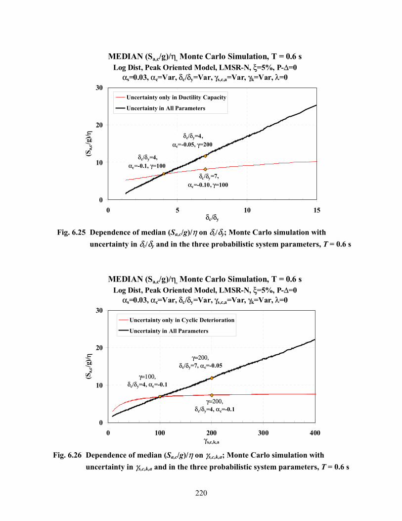
220



0

10

20

30

0 5 10 15δc/δy

(Sa,

c/g)/ η

Uncertainty only in Ductility Capacity


δc/δy=4, αc=-0.05, γ=200

δc/δy=7, αc=-0.10, γ=100

δc/δy=4, αc=-0.1, γ=100

Fig. 6.25 Dependence of median (Sa,c/g)/η on δc/δy; Monte Carlo simulation with

uncertainty in δc/δy and in the three probabilistic system parameters, T = 0.6 s



0

10

20

30

0 100 200 300 400γs,c,k,a

(Sa,

c/g)/ η

Uncertainty only in Cyclic Deterioration


γ=100, δc/δy=4, αc=-0.1

γ=200, δc/δy=4, αc=-0.1

γ=200, δc/δy=7, αc=-0.05

Fig. 6.26 Dependence of median (Sa,c/g)/η on γs,c,k,a; Monte Carlo simulation with

uncertainty in γs,c,k,a and in the three probabilistic system parameters, T = 0.6 s

221

(Sa/g)/η vs PROBABILITY OF COLLAPSE, T=0.6 sAssumed Log Dist., P. O. Model, LMSR-N, ξ=5%, P-∆=0

αs=0.03, αc=-0.10, δc/δy=4, γs,c,k,a=100

0

0.2

0.4

0.6

0.8

1

0 5 10 15(Sa/g) / η

Prob

abili

ty o

f Col

laps

e

Counted DistributionFitted Lognormal Distribution

Uncertainty only in Post-Capping Stiffness

Fig. 6.27 Comparison of fragility curves obtained from counted and fitted

lognormal distributions of 2)(ln , ασ

caS

(Sa/g)/η vs PROBABILITY OF COLLAPSE, T=0.6 sPeak Oriented Model, LMSR-N, ξ=5%, P-∆=0

αs=0.03, αc=-0.10, δc/δy=4, γs,c,k,a=100

0

0.2

0.4

0.6

0.8

1

0 5 10 15 20 25 30(Sa/g) / η

Prob

abili

ty o

f Col

laps

e

Uncertainty in the three Parameters

Uncertainty only in Post-Capping Stiffness

Fig. 6.28 Fragility curves from fitted lognormal distributions for 2

)(ln , ασcaS and 2

)(ln , XS caσ

222

VAR[ln Sa,c(Xi)], FOSM & MONTE CARLO METHODS σlnXi=0.60, ρi,j=1.0, P.O. Model, LMSR-N, ξ=5%, P-∆=0,


0

0.2

0.4

0.6


Var

[ln S

a,c(X

i)]

σFOSM, 0.6 = 0.215σMC, 0.6 = 0.217 σFOSM, 1.8 = 0.329

σMC, 1.8 = 0.304


)(ln , ica XSσ obtained with FOSM (solid lines) and Monte Carlo simulation, reference system, full correlation

(Sa/g)/η at COLLAPSE vs αc, T = 0.5 sPeak Oriented Model, LMSR-N, ξ=5%, P-∆=0, αs=0.03, αc=Var, δc/δy=4, γs,c,a=100, γk=200, λ=0

ln(Sa/η) = 1.101exp[-0.203*ln(-αc)]R2 = 0.994

1

1.5

2

2.5

-4 -3 -2 -1 0ln(-αc)

ln (S

a/g)/ η

(Sa/g)/η at COLLAPSE vs αc, T = 0.5 sPeak Oriented Model, LMSR-N, ξ=5%, P-∆=0, αs=0.03, αc=Var, δc/δy=4, γs,c,a=100, γk=200, λ=0

ln(Sa,c/g)/η = -0.36 ln(-αc) + 0.939R2 = 0.9836

1

1.5

2

2.5

-4 -3 -2 -1 0ln(-αc)

ln(S

a,c/g

)/ η

(a) Fitting with Exponential Curve (b) Linear Regression

Fig. 6.30 Regression for dependence of (Sa,c/g)/η on αc at T = 0.5 s, reference SDOF system

223

MONTE CARLO SIMULATION, T=0.5 sPeak Oriented Model, LMSR-N, ξ=5%, P-∆=0, αs=0.03, αc=Var, δc/δy=4, γs,c,a=100, γk=200, λ=0

0

200

400

600

800

1000

1200

1400

1

Freq

uenc

y

Var[ln Sa,c(α)]MC =0.0465Var[ln Sa,c(α)]FOSM=0.0459

x50

ln(5.85)

ln [(Sa,c/g)/η]x16 x84

Fig. 6.31 Histogram of 2

)(ln , ασcaS from Monte Carlo simulation; reference SDOF

system, T = 0.5 s

Var[ln Sa,c(α)] / Var[ln Sa,c(RTR)] RATIOSPeak Oriented Model, LMSR-N, ξ=5%, P-∆=0, αs=0.03, αc=-0.10, δc/δy=4, γs,c,a=100, γk=200, λ=0

0%

50%

100%

150%

200%


Var

[ln S

a,c( α

)] /

Var

[ln S

a,c(R

TR

)] FOSM Method

Approx. of Variance withLinear Regression


)(ln2

)(ln ,,/ RTRSS cacaσσ α ratios for FOSM method and

approximation from linear regression, reference SDOF system

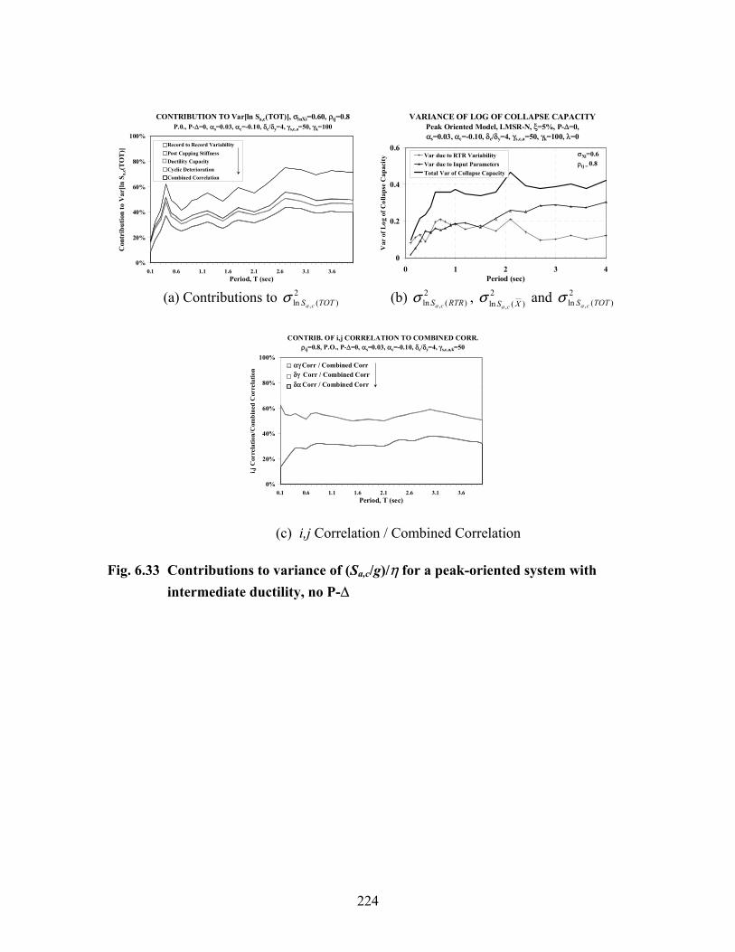
224

CONTRIBUTION TO Var[ln Sa,c(TOT)], σlnXi=0.60, ρij=0.8

P.0., P-∆=0, αs=0.03, αc=-0.10, δc/δy=4, γs,c,a=50, γk=100

0%

20%

40%

60%

80%

100%

0.1 0.6 1.1 1.6 2.1 2.6 3.1 3.6Period, T (sec)

Con

trib

utio

n to

Var

[ln S

a,c(T

OT

)]


VARIANCE OF LOG OF COLLAPSE CAPACITYPeak Oriented Model, LMSR-N, ξ=5%, P-∆=0, αs=0.03, αc=-0.10, δc/δy=4, γs,c,a=50, γk=100, λ=0

0

0.2

0.4

0.6


Var

of L

og o

f Col

laps

e C

apac

ity

Var due to RTR VariabilityVar due to Input ParametersTotal Var of Collapse Capacity

σXi=0.6ρij = 0.8

(a) Contributions to 2

)(ln , TOTS caσ (b) 2



)(ln , TOTS caσ

CONTRIB. OF i,j CORRELATION TO COMBINED CORR.

ρij=0.8, P.O., P-∆=0, αs=0.03, αc=-0.10, δc/δy=4, γs,c,a,k=50

0%

20%

40%

60%

80%

100%

0.1 0.6 1.1 1.6 2.1 2.6 3.1 3.6Period, T (sec)

i,j C

orre

latio

n/C

ombi

ned

Cor

rela

tion

αγ Corr / Combined Corrδγ Corr / Combined Corr δα Corr / Combined Corr

(c) i,j Correlation / Combined Correlation

Fig. 6.33 Contributions to variance of (Sa,c/g)/η for a peak-oriented system with intermediate ductility, no P-∆

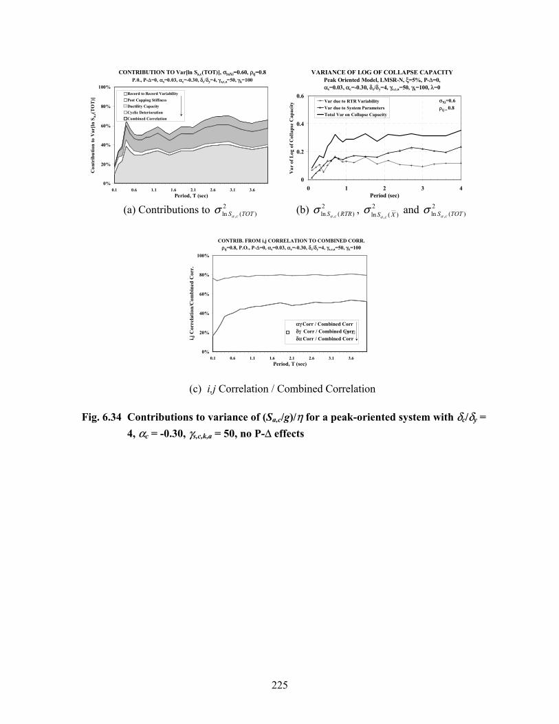
225

CONTRIBUTION TO Var[ln Sa,c(TOT)], σlnXi=0.60, ρij=0.8P.0., P-∆=0, αs=0.03, αc=-0.30, δc/δy=4, γs,c,a=50, γk=100

0%

20%

40%

60%

80%

100%

0.1 0.6 1.1 1.6 2.1 2.6 3.1 3.6Period, T (sec)

Con

trib

utio

n to

Var

[ln S

a,c(T

OT

)]Record to Record VariabilityPost Capping StiffnessDuctility CapacityCyclic DeteriorationCombined Correlation


0

0.2

0.4

0.6


Var

of L

og o

f Col

laps

e C

apac

ity

Var due to RTR VariabilityVar due to System ParametersTotal Var on Collapse Capacity

σXi=0.6ρij = 0.8





)(ln , TOTS caσ

CONTRIB. FROM i,j CORRELATION TO COMBINED CORR.

ρij=0.8, P.O., P-∆=0, αs=0.03, αc=-0.30, δc/δy=4, γs,c,a=50, γk=100

0%

20%

40%

60%

80%

100%

0.1 0.6 1.1 1.6 2.1 2.6 3.1 3.6Period, T (sec)

i,j C

orre

latio

n/C

ombi

ned

Cor

r.

αγ Corr / Combined Corrδγ Corr / Combined Corr δα Corr / Combined Corr

(c) i,j Correlation / Combined Correlation

Fig. 6.34 Contributions to variance of (Sa,c/g)/η for a peak-oriented system with δc/δy = 4, αc = -0.30, γs,c,k,a = 50, no P-∆ effects

226

CONTRIBUTION TO Var[ln Sa,c(TOT)], σlnXi=0.60, ρij=0.8P.0., P-∆=0, αs=0.03, αc=-0.30, δc/δy=2, γs,c,a=25, γk=50

0%

20%

40%

60%

80%

100%

0.1 0.6 1.1 1.6 2.1 2.6 3.1 3.6Period, T (sec)

Con

trib

utio

n to

Var

[ln S

a,c(T

OT



0

0.2

0.4

0.6


Var

of L

og o

f Col

laps

e C

apac

ity

Var due to RTR Variability

Var due to Input Parameters

Total Var on Collapse Capacity

σXi=0.6ρij = 0.8





)(ln , TOTS caσ

Fig. 6.35 Contributions to variance of (sa,c/g)/η for a peak-oriented system with low ductility, no P-∆


P.0., P-∆=0, αs=0.03, αc=-0.10, δc/δy=6, γs,c,a=100, γk=200

0%

20%

40%

60%

80%

100%

0.1 0.6 1.1 1.6 2.1 2.6 3.1 3.6Period, T (sec)

Con

trib

utio

n to

Var

[ln S

a,c(T

OT

)]



0

0.2

0.4

0.6


Var

of L

og o

f Col

laps

e C

apac

ity Var due to RTR Variability



σXi=0.6ρij = 0.8





)(ln , TOTS caσ

Fig. 6.36 Contributions to variance of (sa,c/g)/η for a peak-oriented system with high ductility, no P-∆

CONTRIBUTION TO Var[ln Sa,c(TOT)], σlnXi=0.60, ρij=0.8Bilinear, P-∆=0, αs=0.03, αc=-0.10, δc/δy=4, γs,c,a=50, γk=100

0%

20%

40%

60%

80%

100%

0.1 0.6 1.1 1.6 2.1 2.6 3.1 3.6Period, T (sec)

Con

trib

utio

n to

Var

[ln S

a,c(T

OT

)]


VARIANCE OF LOG OF COLLAPSE CAPACITYBilinear Model, LMSR-N, ξ=5%, P-∆=0,


0

0.2

0.4

0.6


Var

of L

og o

f Col

laps

e C

apac


Var due to Input ParametersTotal Var on Collapse Capacity

σXi=0.6ρij = 0.8





)(ln , TOTS caσ

Fig. 6.37 Contributions to variance of (sa,c/g)/η for a bilinear system with intermediate ductility, no P-∆

227

CONTRIBUTION TO Var[ln Sa,c(TOT)], σlnXi=0.60, ρij=0.8P.0., P-∆=0.1N, αs=0.03, αc=-0.10, δc/δy=4, γs,c,a=50, γk=100

0%

20%

40%

60%

80%

100%

0.1 0.6 1.1 1.6 2.1 2.6 3.1 3.6Period, T (sec)

Con

trib

utio

n to

Var

[ln S

a,c(T

OT


VARIANCE OF LOG OF COLLAPSE CAPACITYPeak Oriented Model, LMSR-N, ξ=5%, P-∆='0.1N',


0

0.2

0.4

0.6


Var

of L

og o

f Col

laps

e C

apac

ity


σXi=0.6ρij = 0.8





)(ln , TOTS caσ

Fig. 6.38 Contributions to variance of (sa,c/g)/η for a peak-oriented system with intermediate ductility, small P-∆


P.0., P-∆='0.1N', αs=0.03, αc=-0.30, δc/δy=4, γs,c,a=50, γk=100

0%

20%

40%

60%

80%

100%

0.1 0.6 1.1 1.6 2.1 2.6 3.1 3.6Period, T (sec)

Con

trib

utio

n to

Var

[ln S

a,c(T

OT)

]




0

0.2

0.4

0.6


Var

of L

og o

f Col

laps

e C

apac

ity


σXi=0.6ρij = 0.8





)(ln , TOTS caσ

Fig. 6.39 Contributions to variance of (Sa,c/g)/η for a peak-oriented system with δc/δy = 4, αc = -0.30, γs,c,k,a = 50, small P-∆


0%

20%

40%

60%

80%

100%

0.1 0.6 1.1 1.6 2.1 2.6 3.1 3.6Period, T (sec)

Con

trib

utio

n to

Var

[ln S

a,c(T

OT)

]




0

0.2

0.4

0.6


Var

of L

og o

f Col

laps

e C

apac




σXi=0.6ρij = 0.8





)(ln , TOTS caσ

Fig. 6.40 Contributions to variance of (sa,c/g)/η for a peak-oriented system with low ductility, small P-∆

228


0%

20%

40%

60%

80%

100%

0.1 0.6 1.1 1.6 2.1 2.6 3.1 3.6Period, T (sec)

Con

trib

utio

n to

Var

[ln S

a,c(T

OT




0

0.2

0.4

0.6


Var

of L

og o

f Col

laps

e C

apac

ity

Var due to RTR Variability



σYi=0.6ρij = 0.8





)(ln , TOTS caσ

Fig. 6.41 Contributions to variance of (sa,c/g)/η for a peak-oriented system with high ductility, small P-∆


Bilinear, P-∆=0.1N, αs=0.03, αc=-0.10, δc/δy=4, γs,c,a=50, γk=100

0%

20%

40%

60%

80%

100%

0.1 0.6 1.1 1.6 2.1 2.6 3.1 3.6Period, T (sec)

Con

trib

utio

n to

Var

[ln S

a,c(T

OT

)]


VARIANCE OF LOG OF COLLAPSE CAPACITYBilinear Model, LMSR-N, ξ=5%, P-∆='0.1N',


0

0.2

0.4

0.6


Var

of L

og o

f Col

laps

e C

apac


Var due to Input ParametersTotal Var on Collapse Capacity

σXi=0.6ρij = 0.8





)(ln , TOTS caσ

Fig. 6.42 Contributions to variance of (sa,c/g)/η for a bilinear system with

intermediate ductility, small P-∆

229

CONTRIBUTION TO Var[ln Sa,c(TOT)], σlnXi=0.60, ρij=0.8P.0., T1=0.1N, BH, αs=0.03, αc=-0.10, δc/δy=4, γs,c,a=50, γk=100

0%

20%

40%

60%

80%

100%

0.3 0.6 0.9 1.2 1.5 1.8Period, T (sec)

Con

trib

utio

n to

Var

[ln S

a,c(T

OT

)]RTR VariabilityPost Capping StiffnessDuctility CapacityCyclic DeteriorationCombined Correlation

0%

20%

40%

60%

80%

100%

0.1 0.6 1.1 1.6 2.1 2.6 3.1 3.6

SDOF System

Fig. 6.43 Contributions to 2

)(ln , TOTS caσ for set of MDOF systems with T = 0.1N and

springs at ends of beams with intermediate ductile characteristics

CONTRIB. OF i,j CORRELATION TO COMBINED CORR. ρij=0.8, P.O., T1=0.1N, αs=0.03, αc=-0.10, δc/δy=4, γs,c,a=50, γk=100

0%

20%

40%

60%

80%

100%

0.3 0.6 0.9 1.2 1.5 1.8Period, T (sec)

i,j C

orre

latio

n/C

ombi

ned

Cor

r

αγ Corr. / Combined Corr.δγ Corr. / Combined Corr.δα Corr. / Combined Corr.

Fig. 6.44 i,j correlation / combined correlation for set of MDOF systems with T = 0.1N

and springs at ends of beams with intermediate ductile characteristics

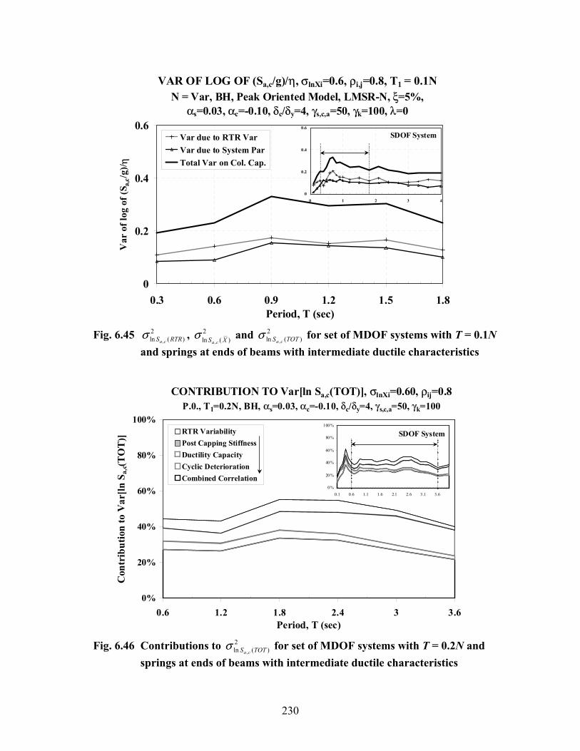
230

VAR OF LOG OF (Sa,c/g)/η, σlnXi=0.6, ρi,j=0.8, T1 = 0.1NN = Var, BH, Peak Oriented Model, LMSR-N, ξ=5%,


0

0.2

0.4

0.6

0.3 0.6 0.9 1.2 1.5 1.8Period, T (sec)

Var

of l

og o

f (S a

,c/g

)/ ηVar due to RTR VarVar due to System ParTotal Var on Col. Cap.

0

0.2

0.4

0.6

0 1 2 3 4

SDOF System

Fig. 6.45 2



)(ln , TOTS caσ for set of MDOF systems with T = 0.1N


CONTRIBUTION TO Var[ln Sa,c(TOT)], σlnXi=0.60, ρij=0.8P.0., T1=0.2N, BH, αs=0.03, αc=-0.10, δc/δy=4, γs,c,a=50, γk=100

0%

20%

40%

60%

80%

100%

0.6 1.2 1.8 2.4 3 3.6Period, T (sec)

Con

trib

utio

n to

Var

[ln S

a,c(T

OT

)]

RTR VariabilityPost Capping StiffnessDuctility CapacityCyclic DeteriorationCombined Correlation

0%

20%

40%

60%

80%

100%

0.1 0.6 1.1 1.6 2.1 2.6 3.1 3.6

SDOF System

Fig. 6.46 Contributions to 2



231

CONTRIB. OF i,j CORRELATION TO COMBINED CORR. ρij=0.8, P.O., T1=0.2N, αs=0.03, αc=-0.10, δc/δy=4, γs,c,a=50, γk=100

0%

20%

40%

60%

80%

100%

0.6 1.2 1.8 2.4 3 3.6Period, T (sec)

i,j C

orre

latio

n/C

ombi

ned

Cor

r.αγ Corr. / Combined Corr.δγ Corr. / Combined Corr.δα Corr. / Combined Corr.

Fig. 6.47 i,j correlation / combined correlation for set of MDOF systems with T = 0.2N


VAR. OF LOG OF (Sa,c/g)/η, σlnXi=0.6, ρi,j=0.8, T1 = 0.2NN = Var, BH, Peak Oriented Model, LMSR-N, ξ=5%,


0

0.2

0.4

0.6

0.6 1.2 1.8 2.4 3 3.6Period

Var

of L

og o

f (S a

,c/g

)/η

Var due to RTR VarVar due to System ParTotal Var on Col. Cap

0

0.2

0.4

0.6

0 1 2 3 4

SDOF System

Fig. 6.48 2





7 Fragility Curves and Mean Annual Frequency of Collapse

7.1. INTRODUCTION

In seismic performance assessment, collapse constitutes one of several limit states of interest,

such as a limit state that contributes to the cost of damage, if monetary losses or downtime are

performance targets. In this context collapse could be viewed as a damage measure for which it

is useful to develop fragility curves (FCs). In addition, collapse is the main source of casualties

and loss of lives. In this context, collapse is an intermittent decision variable that could be

described by the mean annual frequency (MAF).

This chapter explores alternatives for representing FCs based on computed collapse

capacities and the effect that different system properties have on these curves. Previous to the

presentation of the MAF of collapse, approximated hazard curves (HCs) for a specific site are

introduced, which are derived from equal hazard spectra. Numerical integration is used for

combining the FCs and HCs to obtain the MAF of collapse for a given site. The advantages of

computing the MAF of collapse by using FCs derived directly from collapse capacities instead of

EDPs associated with collapse are discussed.

1.1 7.2 COLLAPSE FRAGILITY CURVES (FCs)

A fragility function for a limit state expresses the conditional probability of exceeding the limit

state capacity for a given level of ground motion intensity. The objective of this study is to

evaluate the limit state of collapse by using the spectral acceleration at the fundamental period of

the system as the ground motion intensity. Thus, the FC for these conditions is:

][][)( ,,, ,xSPxSSSPxF caacaaSC ca

≤==≥= (7.1)

234

)(,, xFcaSC corresponds to the value of the fragility curve (FC) at spectral acceleration, x,

for the limit state of collapse, i.e., the “collapse fragility curve.” By considering that the demand

(Sa = x) is statistically independent of the capacity of the system (Sa,c), the FC can be expressed

as the probability that Sa,c is less than or equal to x. The collapse FC can be viewed also as the

cumulative distribution function (CDF) of a random variable, the collapse capacity, Sa,c.

In previous chapters, “collapse capacity” has been used as the parameter for collapse

evaluation. This normalized parameter is defined as the ratio of the ground motion intensity to a

structural strength parameter when collapse occurs ([(Sa/g)/η]c for SDOF systems and

{[Sa(T1)/g]/γ}c for MDOF systems23]. Therefore, it is possible to generate “normalized collapse

fragility curves” by using this normalized parameter instead of the ground motion intensity. For

SDOF systems, normalized collapse FCs are obtained by modifying Equation 7.1 as follows:

]/)/[()( ,/)/(, ,xgSPxF cagSC ca

≤= ηη (7.2)

One of the advantages of assessing collapse based on the relative intensity (collapse

capacity) is that the parameter can be easily de-normalized and plugged directly in Equation 7.1

(see Section 7.2.4.).

7.2.1 Normalized Counted Collapse Fragility Curves

Counted collapse fragility curves are obtained by treating the collapse capacity data as a random

sample, i.e., equally likely outcomes. For instance, if the limit state of collapse is evaluated for a

system subjected to 40 ground motions, the probability of collapse increases by 1/40 (0.025)

after each individual collapse occurs.

Data of the type shown in Figure 2.4 are utilized to develop normalized collapse fragility

curves, which describe the probability of collapse given the value of (Sa/g)/η (or [Sa(T1)/g]/γ for

MDOF systems). Typical results of counted fragility curves are presented in Figure 7.1a for

SDOF systems of various periods but with the same baseline hysteretic properties:

• Peak-oriented model

• Medium ductility capacity, δc/δy = 4

23 For the sake of simplicity, collapse capacity is also expressed as (Sa,c/g)/η for SDOF systems and

[Sa,c(T1)/g]/γ for MDOF systems.

235

• Small post-capping stiffness, αc = -0.10

• No cyclic deterioration, γs,c,k,a = infinite

As observed, normalized collapse fragility curves are very similar for SDOF systems

with these hysteresis properties and periods longer than about T = 0.6 s. This is expected from

observing that median collapse capacities for SDOF systems with P-∆ = 0.1N are essentially

period independent for periods longer than about T = 0.6 s (Fig. 4.32a). Figure 7.1b presents

fragility curves for systems with the same natural period T = 0.6 s, but different hysteretic

properties. As can be seen, probability of collapse is very sensitive to hysteretic properties.

7.2.2 Normalized Collapse Fragility Curves Obtained by Fitting Lognormal Distribution to Data

Counted FCs are based on the real distribution of the sample data but are difficult to incorporate

into analytical formulations. For this reason, a lognormal distribution is fitted to collapse

capacity data and, although it is an approximation of the distribution of the sample data, it

facilitates numerical and analytical calculations. The lognormal distribution is a logical selection

for several reasons: (a) most of the individual collapse capacity data have a skewed distribution

with a longer tail for upper values (Fig. 2.4 and 2.5 and Appendix C for a goodness-of-fit test),

(b) collapse capacity values are always positive and, (c) previous studies have associated the

distribution of spectral acceleration and the response of a nonlinear structure (in terms of EDPs)

to lognormal distributions (Shome and Cornell, 1999).

Figure 7.2 presents FCs for different SDOF systems. The irregular curves are obtained

from the ordered data points (counted FCs), whereas the smooth curves are the result of fitting a

lognormal distribution to the data, which fits the data rather well. For this reason in the

subsequent graphs for MDOF frames only the fitted distributions are shown.

The dependence of the fragility curves on the system period is presented in Figure 7.2a

for SDOF systems with baseline hysteretic properties. As observed, for a given relative intensity

the systems with short period have a higher probability of collapse. On the other hand, Figure

7.2b presents FCs for SDOF systems with the same elastic period (T = 0.6 s.) but different

hysteretic properties. This figure shows the large sensitivity of the probability of collapse to the

hysteretic properties, emphasizing the importance of “ductility” in the prevention of collapse.

236

The FCs of Figure 7.2b can be used for obtaining collapse capacity ratios for different

probabilities of collapse, i.e., over the entire range of probabilities of collapse, the relative

intensity of each FC is normalized by the relative intensity of the FC corresponding to the most

ductile system (Fig. 7.3). The collapse capacity ratios obtained from the counted FCs are

essentially independent of the probability of collapse in the range of 0.20–0.80. This indicates

that the dispersion in the collapse capacity is approximately the same for each case. This

observation may justify the extrapolation of the conclusions obtained from median collapse

capacities ratios in Chapters 4 and 5 to other probabilities of collapse. In the case of the collapse

capacity ratios obtained from fitted lognormal distributions, there is a clear pattern of a decrease

in collapse capacity ratios for higher probabilities of collapse. In any case, the aforementioned

extrapolation still would be feasible because the difference between the collapse capacity ratios

at the probability of collapse of 0.50 and probabilities of collapse in the range from 0.20–0.80 is

relatively small.

7.2.3 De-normalization of Collapse Fragility Curves

In most of this study, collapse capacities are based on the maximum relative intensity (Sa/g)/η

(or [Sa(T1)/g]/γ for MDOF systems) that the system may resist. However, to compute the MAF

of collapse, these curves need to be de-normalized by a specific strength of the structural system.

That is to say, the structural strength parameter (γ or η) should remain constant. As an

illustration, Figure 7.4 presents de-normalized FCs for an SDOF system with baseline hysteretic

properties under different base shear strengths. As can be seen, for a given probability of

collapse the spectral acceleration at collapse decreases proportionally to the decrease in the

strength of the system. Observe that for large shear strength values it is possible to anticipate

small values of the MAF of collapse. For instance, for the system with η = 1, the probability of

collapse is only of about 5% at the very large spectral acceleration Sa/g = 3. Therefore, the

combination of this FC with any reasonable HC for a given site will result in a low MAF of

collapse because the annual rate of exceedance of a ground motion with Sa/g ≥ 3 will be very

small.

237

7.2.4 Collapse Fragility Curves for MDOF Frames with Parameter Variations

Figure 7.5 presents FCs for MDOF systems that can be compared directly to the SDOF fragility

curves of Figure 7.2a. These curves are obtained for generic frames with beam-hinge

mechanism, in which the hysteretic properties of the springs at the end of the beams correspond

to the baseline structural properties (see Chapter 5 for a description of the generic frames). The

four-digit code identifies the number of stories and the first mode period of each frame, i.e., 0918

means a 9-story frame with T1 = 1.8 s.

Figure 7.5 shows a pattern equivalent to that exhibited in the median collapse capacity

spectra of MDOF systems (Chapter 5), of high fragility (small collapse capacity) for short period

structures (T1 = 0.3 s.), a large decrease in the fragility for medium period structures (T1 = 0.6

and 0.9 s.), and then an increase in fragility for long-period structures (T1 = 1.8 and 3.6 s.)

because of the predominance of P-∆ effects.

The effects of ductility capacity and post-capping tangent stiffness are illustrated in

Figures 7.6–7.7 for four frames with the first mode period varying from 0.3 s–3.6 s. An increase

in the ductility capacity shifts the fragility curves to the right, but not by an amount proportional

to the increase in ductility capacity. An increase in the slope of the post-capping tangent stiffness

(from flat to steep) has a very detrimental effect on the fragility.

In concept, all observations that have been made previously for median collapse

capacities hold true for the FCs. The value of these curves lies in their probabilistic nature that

permits probabilistic expressions of performance and design decisions. For instance, if for a

given long return period hazard (e.g., 2/50 hazard) a 10% probability of collapse could be

tolerated, then the intersections of a horizontal line at a probability of 0.1 with the individual

fragility curves provides targets for the R-factor that should be employed in design, in

conjunction with the spectral acceleration associated with this hazard. If such horizontal lines are

drawn in the graphs of Figures 7.6–7.7, it can be conjectured that the indicated R-values are low,

even for rather ductile systems.

The second value of the fragility curves lies in the opportunity they provide for a rigorous

computation of the MAF of collapse.

238

1.2 7.3 SPECTRAL ACCELERATION HAZARD

Information about the seismic hazard is necessary in order to obtain the MAF of collapse.

Generally seismic hazard is reported in terms of 5%-damped spectral acceleration at the

fundamental period of the system, )( 1TSa , which becomes the ground motion intensity measure

(IM). Hazard curves (HCs) report the mean annual frequency of exceeding a particular spectral

acceleration for a given period and damping ratio.

Seismologists usually provide spectral acceleration hazard curves for a given site. This

information may be approximated by a power-law relationship in the region of interest (FEMA

355C, 2000; Luco, 2002; Jalayer, 2003):

[ ] koIM xkxIMPx −=≥=)(λ (7.3)

or specifically:

[ ] kaoaaaTS SkSTSPS

a

−=≥= )()( 1)( 1λ (7.4)

)()( 1 aTS Sa

λ is defined here as the MAF of the ground motion having a spectral response

acceleration at the fundamental period of the system greater than Sa. For the small probabilities

of interest here it is numerically equal to the annual probability of exceedance. The parameter ko

is a constant that depends on the seismicity of the site and k approximates the local slope of the

hazard curve, in the log domain, around the return period of interest. The slope of the hazard

curve is a function of the hazard level, location and response period.

To illustrate the computation of MAF of collapse, HCs for various periods are

approximated from the equal hazard spectra employed in PEER studies for a Los Angeles

building (Somerville and Collins, 2002) (Fig. 7.8). The equal hazard spectra for the site were

derived from the USGS probabilistic ground motion maps for rock site conditions. Spectra for

soil site conditions were generated from the rock site spectra by using the Abrahamson and Silva

(1997) ground motion model. These curves represent an equal probability of exceeding the

ground motion at any period for 50/50, 10/50, and 2/50 hazard levels. The hazard levels are

based on a probability of exceedance in a 50-year period. For instance, 10/50 refers to the

probability of exceedance of 10% in 50 years (1/475).

The values at each period are used to derive power-law relationships of the type of

Equation 7.2. Several reasonable approaches could be proposed for this purpose. The simplest

one is to approximate the hazard curve in the region of interest with a straight line in the log-log

239

domain of spectral acceleration and probability of exceedance. A linear regression analysis is

used to fit the straight line (Fig. 7.9). The use of the three hazard levels “averages” the

probability of exceedance over all the possible spectral acceleration values, which is convenient

for the example of Section 7.4 because the region of interest for the MAF of collapse changes

according to the period and the ductility characteristics of the system.

Figure 7.10 presents some of the hazard curves derived from the equal hazard spectra. As

can be seen, the annual frequency of exceedance has reasonable limits even for small spectral

accelerations, which usually does not occur when the approximation is made only with the 10/50

and 2/50 hazard levels. However, note that the probabilities of exceedance of the approximated

HCs may be overestimated for large spectral accelerations because the linear regression flattens

the HCs in this region. For this reason, in the computation of the MAF of collapse, the HCs are

terminated at Sa/g = 3.

1.3 7.4 MEAN ANNUAL FREQUENCY OF GLOBAL COLLAPSE

7.4.1 Formulation

The MAF of collapse ( cλ ) can be calculated once the de-normalized FCs of the system and HCs

for the site of interest are known. The MAF of collapse is expressed as the mean annual

frequency of the strong motion intensity (Sa) being larger than the collapse capacity (expressed

as a function of Sa,c given η) multiplied by the probability of having such a strong motion

intensity:

∫∞

=>=0

, ).(.].[ dxxfvxSSSPaSacaacλ (7.5)

where, )(xfaS is the probability density function (PDF) at the spectral acceleration value x given

an event of interest, and v represents the annual rate of the occurrence of such events (rate of

seismicity). In Section 7.2 the first term of the integral was defined as the collapse fragility

curve. Therefore:

∫∞

=0

, ).(.).(,

dxxfvxFaca SSCcλ (7.6)

240

The PDF of the spectral acceleration value can be expressed in terms of the

complementary cumulative distribution (CCDF) function (Jalayer, 2003):

dxxdG

xf a

a

SS

)()( = (7.7)

In this equality, the CCDF [ )(xGaS ] is the probability of exceeding a certain value, whereas the

CDF [ )()()( xdxfxFaa SS = ] is the probability of being less than or equal to a certain threshold.

Therefore, their corresponding derivatives are equal in absolute values but have opposite signs.

By substituting Equation 7.7 in 7.6:

∫∞

=0

, )(.).(,

xdGvxFaca SSCcλ (7.8)

In addition, the spectral acceleration hazard, )(xd Saλ , is equal to:

)(.)( xdGvxdaSa =λ (7.9)

by substituting Equation 7.9 in 7.8:

∫∞

=0

, )().(,

xdxF aSCc caλλ (7.10)

Equation 7.10 explicitly expresses the MAF of collapse in terms of the collapse fragility curve

for a given median base shear strength over a Sa hazard curve pertaining to a specific site. The

process of integrating Equation 7.10 has been illustrated graphically in Figure 2.10.

Note that this approach is more straightforward than the methodology for computing

collapse based on displacement demands and capacities. The “EDP-based approach”

decomposes the collapse limit state into two steps and requires an additional integration (Jalayer,

2003). First, the EDP hazard is obtained as the probability of exceeding a demand threshold

given that the IM is equal to a certain value, x. In a second step, the probability of collapse is

obtained as the likelihood of having an EDP demand hazard larger than the EDP capacity. Thus,

it is concluded that the evaluation of global collapse based on the relative intensity of the system

facilitates the computation of the mean annual frequency of collapse.

241

7.4.2 Computation of Mean Annual Frequency of Collapse for a Specific Site, SDOF Systems

The example presented in this section illustrates the methodology to compute the MAF of

collapse for various periods and selected strength levels, η. It also permits a gross quantification

of the effect of several parameters on the MAF of collapse.

Collapse FCs for SDOF systems with baseline hysteretic properties and P-∆ = 0.1N are

shown in Figure 7.11 for different periods and for a yield strength coefficient η = 0.2. As can be

seen, in the period range of T = 0.1 to 2.0 s, the longer the period the larger the spectral

acceleration that leads to collapse for a given probability of collapse. This fact will be reflected

in smaller MAF of collapse for SDOF systems with longer periods.

The FCs of Figure 7.11 and the HCs obtained from the equal hazard spectra (Section 7.3)

are utilized for solving Equation 7.10 by numerical integration. The result of this integration is

represented graphically in Figure 7.12, where a curve for MAF of collapse due to xSa = is

obtained for T = 0.5 s. Figure 7.13 shows more of these curves for systems with different

periods. The diamonds on the FCs of Figure 7.11 indicate the spectral acceleration at which the

peaks of the curves for MAF of collapse due to xSa = occur. For this example, all the peaks are

located at the spectral acceleration region at which the FC begins to build up, and where the

probability of collapse is about 0.20.

The areas under the curves of Figure 7.13 corresponds to the MAFs of collapse, which

are plotted in Figure 7.14 for several periods and different strengths for SDOF systems with the

baseline hysteretic properties. The MAFs of collapse illustrate general trends and are the product

of a rigorous computational process. Observe that the MAF of collapse may differ by several

orders of magnitude for systems with the same properties but different yield strength.

A comparison of MAFs of collapse for systems of different hysteretic properties, given

η = 0.2, is presented in Figure 7.15. The figure shows that the MAF of collapse can increase by

more than one order of magnitude due to the ductile characteristics of the system. Figures 7.14–

7.15 show a strong dependence of the MAF of collapse on the natural period of SDOF systems

with otherwise identical properties.

Effect of Uncertainty in System Parameters. An SDOF system with baseline properties

but γs,c,k,a = 50 is utilized for computing the MAF of collapse including uncertainty in system

242

parameters. Figure 6.33 presents the contribution of uncertainty in system parameters to variance

of collapse capacity for the aforementioned system. This contribution can be larger than that due

to RTR variability. The MAF of collapse for this system is presented for different periods and

two different strengths in Figure 7.16. As can be seen, the additional variance increases the MAF

of collapse by about 50–100% compared with the case where RTR variability is the only source

of uncertainty.

The total variance in collapse capacity due to RTR variability and uncertainty in the input

parameters may increase the MAF of collapse several times. Figure 7.17 presents MAFs of

collapse for the former systems with η = 0.2, considering deterministic SDOF systems, systems

with dispersion due to RTR variability, and systems with dispersion due to RTR variability plus

uncertainty in the system parameters. If it were possible to calculate the collapse capacity of the

system in a deterministic way, the MAF of collapse would decrease by more than a factor of four

at some periods.

7.4.3 Computation of Mean Annual Frequency of Collapse for a Specific Site, MDOF Systems

The study of MAF of collapse for the generic frames of Chapter 5 is divided into MAFs for stiff

and flexible frames. Figure 7.18 shows the FCs of the stiff frames (T1 = 0.1N) for a base shear

strength γ = 0.2 24. Unlike SDOF systems with P-∆ = 0.1N (small P-∆), the collapse FCs are

sensitive to variations of the fundamental period of the system over the full range of periods of

interest. The main reason for this trend is the large P-∆ effect for systems with long fundamental

period. This phenomenon is not observed in SDOF systems with small P-∆ effects because the

elastic stability coefficient utilized in these systems does not capture the large P-∆ effects of the

generic frames with long fundamental period.

The combination of FCs of Figure 7.18 with the corresponding HCs results in the MAFs

of collapse shown in Figure 7.19 for several strength levels. The curves are for stiff MDOF

systems with beam-hinge mechanism and baseline hysteretic properties in the springs of the

beams. Figures 7.20–7.21 show equivalent FCs and MAFs of collapse but for flexible frames.

24 The fundamental period for some generic frames does not coincide with the periods evaluated by Somerville and Collins. In these cases, the seismic hazard information has been obtained by interpolating the data of the existing periods.

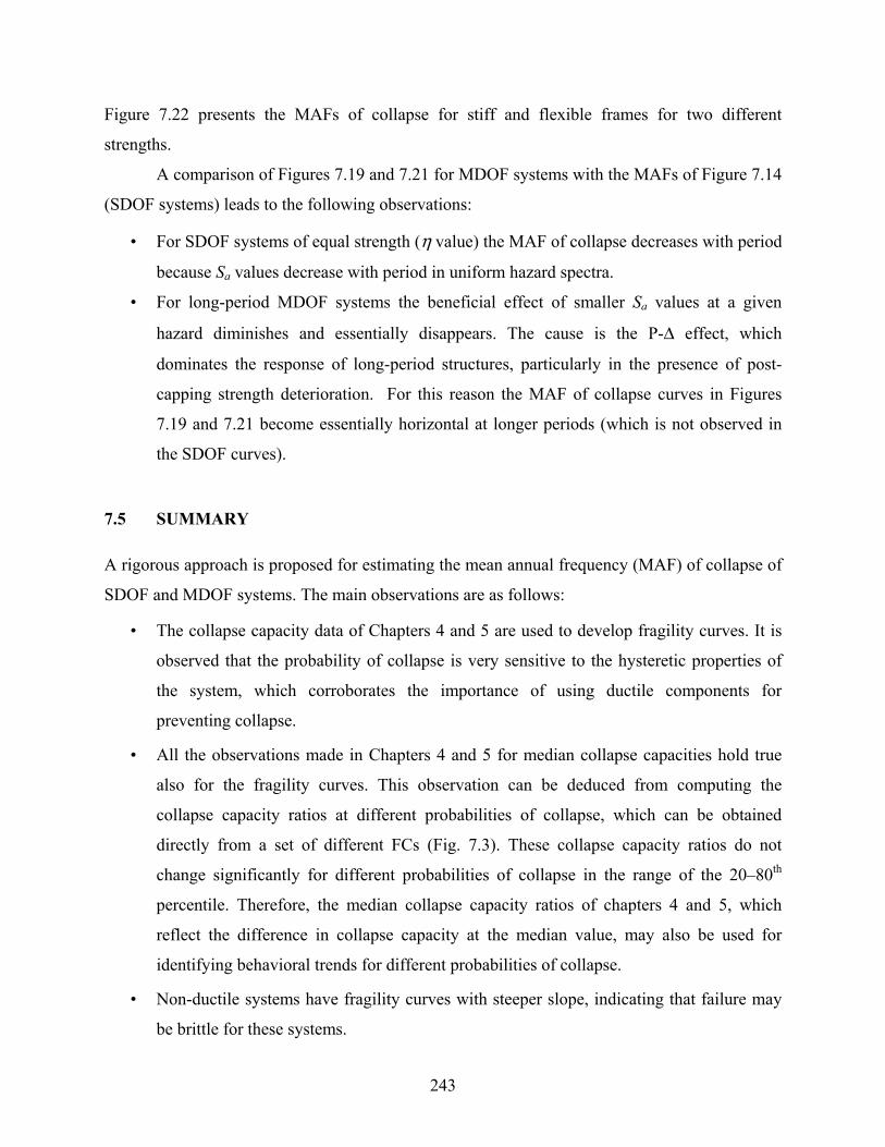
243

Figure 7.22 presents the MAFs of collapse for stiff and flexible frames for two different

strengths.

A comparison of Figures 7.19 and 7.21 for MDOF systems with the MAFs of Figure 7.14

(SDOF systems) leads to the following observations:

• For SDOF systems of equal strength (η value) the MAF of collapse decreases with period

because Sa values decrease with period in uniform hazard spectra.

• For long-period MDOF systems the beneficial effect of smaller Sa values at a given

hazard diminishes and essentially disappears. The cause is the P-∆ effect, which

dominates the response of long-period structures, particularly in the presence of post-

capping strength deterioration. For this reason the MAF of collapse curves in Figures

7.19 and 7.21 become essentially horizontal at longer periods (which is not observed in

the SDOF curves).

1.4 7.5 SUMMARY

A rigorous approach is proposed for estimating the mean annual frequency (MAF) of collapse of

SDOF and MDOF systems. The main observations are as follows:

• The collapse capacity data of Chapters 4 and 5 are used to develop fragility curves. It is

observed that the probability of collapse is very sensitive to the hysteretic properties of

the system, which corroborates the importance of using ductile components for

preventing collapse.

• All the observations made in Chapters 4 and 5 for median collapse capacities hold true

also for the fragility curves. This observation can be deduced from computing the

collapse capacity ratios at different probabilities of collapse, which can be obtained

directly from a set of different FCs (Fig. 7.3). These collapse capacity ratios do not

change significantly for different probabilities of collapse in the range of the 20–80th

percentile. Therefore, the median collapse capacity ratios of chapters 4 and 5, which

reflect the difference in collapse capacity at the median value, may also be used for

identifying behavioral trends for different probabilities of collapse.

• Non-ductile systems have fragility curves with steeper slope, indicating that failure may

be brittle for these systems.

244

• If the spectral acceleration at the first mode period of the system is used as the intensity

measure, then hazard curves can be developed using available seismic hazard

information. The use of such hazard curves in the computation of the MAF of collapse,

and of the collapse capacity information presented in chapters 4 and 5, should give good

results provided the frequency content of the ground motions is insensitive to magnitude

and distance (Medina, 2002; Jalayer, 2003), and provided the ground motions are

representative for the hazard levels that control the MAF of collapse.

• To illustrate the computation of the MAF of collapse, equal hazard spectra are used for

approximating hazard curves at several periods for a given site. A linear regression

analysis is performed at each period with information at the 50/50, 10/50, and 2/50

hazard levels. The obtained hazard curves provide reasonable results for systems of

different periods, strengths and ductility characteristics.

• The potential for global collapse of a frame structure can be expressed probabilistically in

terms of a mean annual frequency of collapse using fragility curves derived from collapse

capacities. The use of this type of FCs results in a straightforward calculation because a

single integration is needed to relate the fragility curve with the seismic hazard of the site.

• The base shear strength of the system is a dominant factor in the magnitude of the MAF

of collapse for a given system. Variations of the base shear strength from η (or γ for

MDOF systems) = 0.5 to 0.1 may produce a difference in the MAF of collapse of more

than two orders of magnitude.

• The MAF of collapse may increase by more than one order of magnitude for non-ductile

systems compared with ductile ones.

• The MAF of collapse for MDOF systems shows the large effect of P-∆ for systems with

longer periods.

• Uncertainty in the system parameters may increase the MAF of collapse by 50–100%

(assuming the dispersions in the parameters of Chapter 6) compared with the cases in

which RTR variability is the only source of uncertainty. For the studied systems, the

MAF of collapse may decrease by more than a factor of four if it were possible to

estimate collapse capacity in a deterministic way.

245

(Sa/g)/η vs PROBABILITY OF COLLAPSEPeak Oriented Model, LMSR-N, ξ=5%, P-∆='0.1N'


0

0.2

0.4

0.6

0.8

1

0 4 8 12 16(Sa/g)/η

Prob

abili

ty o

f Col

laps

e

T = 0.3 s.

T = 0.6 s.

T = 0.9 s.

T = 1.8 s.

(a) Different Periods, Baseline Hysteretic Characteristics

(Sa/g)/η vs PROBABILITY OF COLLAPSE, T=0.6 sPeak Oriented Model, LMSR-N, ξ=5%, P-∆='0.1N'


0

0.2

0.4

0.6

0.8

1

0 4 8 12 16(Sa/g)/η

Prob

abili

ty o

f Col

laps

e


(b) Various Systems, T = 0.6 s

Fig. 7.1 Counted fragility curves for SDOF systems

246

(Sa/g)/η vs PROBABILITY OF COLLAPSEPeak Oriented Model, LMSR-N, ξ=5%, P-∆='0.1N'


0

0.2

0.4

0.6

0.8

1

0 4 8 12 16(Sa/g)/η

Prob

abili

ty o

f Col

laps

e

T = 0.3 s.

T = 1.8 s.

(a) T = 0.3 and 1.8 s, Baseline Hysteretic Properties

(Sa/g)/η vs PROBABILITY OF COLLAPSE, T=0.6 sPeak Oriented Model, LMSR-N, ξ=5%, P-∆='0.1N'


0

0.2

0.4

0.6

0.8

1

0 4 8 12 16(Sa/g)/η

Prob

abili

ty o

f Col

laps

e


(b) Various Systems, T = 0.6 s

Fig. 7.2 Fragility curves for SDOF systems obtained by fitting a lognormal distribution

247

COLLAPSE CAPACITY RATIOS, T=0.5 sPeak Oriented Model, LMSR-N, ξ=5%, P-∆='0.1N'


0

0.2

0.4

0.6

0.8

1

1.2

0 0.2 0.4 0.6 0.8 1Probability of Collapse

Col

laps

e C

apac

ity R

atio

s

γs,c,k,a=Inf, δc/δy=6, αc=-0.10γs,c,k,a=100, δc/δy=4, αc=-0.10 γs,c,k,a=50, δc/δy=4, αc=-0.30 γs,c,k,a=25, δc/δy=2, αc=-0.50

Fig. 7.3 Collapse capacity ratios for different probabilities of collapse, T = 0.5 s

(Sa/g) vs PROBABILITY OF COLLAPSEP.O. Model, LMSR-N, ξ=5%, P-∆='0.1N', T =0.6 sec


0

0.2

0.4

0.6

0.8

1

0 1 2 3 4Sa/g

Prob

abili

ty o

f Col

laps

e

η = 0.1η = 0.2η = 0.5η = 1.0

Fig. 7.4 De-normalization of fragility curves at different base shear strength for SDOF systems; baseline hysteretic properties, T = 0.6 s

248

[Sa(T1)/g]/γ vs PROBABILITY OF COLLAPSEN=Var, T1=Var, BH, Peak Oriented Model, LMSR-N, ξ=5%,


0

0.2

0.4

0.6

0.8

1

0 5 10 15[Sa(T1)/g]/γ

Prob

abili

ty o

f Col

laps

e

030309091818

(a) T1 = 0.1N

[Sa,c(T1)/g]/γ vs PROBABILITY OF COLLAPSEN=Var, T1=Var, BH, Peak Oriented Model, LMSR-N, ξ=5%,


0

0.2

0.4

0.6

0.8

1

0 5 10 15[Sa,c(T1)/g]/γ

Prob

abili

ty o

f Col

laps

e

0306

0918

1836

(b) T1 = 0.2N

Fig. 7.5 Fragility curves for frame structures with springs at beams ends with baseline hysteretic properties

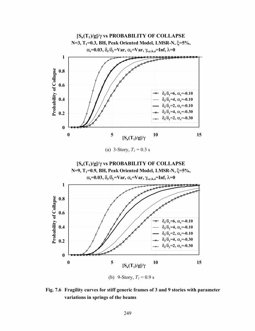
249

[Sa(T1)/g]/γ vs PROBABILITY OF COLLAPSEN=3, T1=0.3, BH, Peak Oriented Model, LMSR-N, ξ=5%,


0

0.2

0.4

0.6

0.8

1

0 5 10 15[Sa(T1)/g]/γ

Prob

abili

ty o

f Col

laps

e

δc/δy=6, αc=-0.10δc/δy=4, αc=-0.10 δc/δy=2, αc=-0.10 δc/δy=4, αc=-0.30 δc/δy=2, αc=-0.30

(a) 3-Story, T1 = 0.3 s



0

0.2

0.4

0.6

0.8

1

0 5 10 15[Sa(T1)/g]/γ

Prob

abili

ty o

f Col

laps

e


(b) 9-Story, T1 = 0.9 s

Fig. 7.6 Fragility curves for stiff generic frames of 3 and 9 stories with parameter variations in springs of the beams

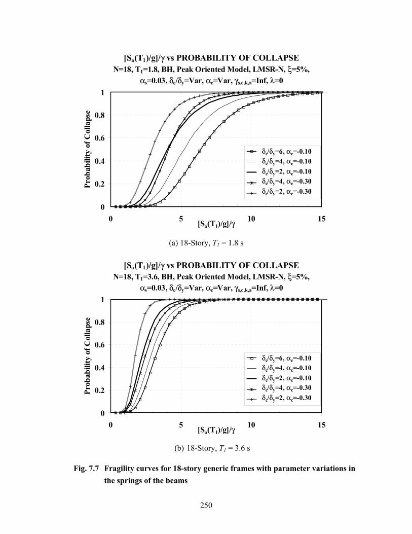
250



0

0.2

0.4

0.6

0.8

1

0 5 10 15[Sa(T1)/g]/γ

Prob

abili

ty o

f Col

laps

e


(a) 18-Story, T1 = 1.8 s



0

0.2

0.4

0.6

0.8

1

0 5 10 15[Sa(T1)/g]/γ

Prob

abili

ty o

f Col

laps

e


(b) 18-Story, T1 = 3.6 s

Fig. 7.7 Fragility curves for 18-story generic frames with parameter variations in the springs of the beams

251

Equal Hazard Spectra, Van Nuys, CA.

0

0.5

1

1.5

2

0 0.5 1 1.5 2Period, T (sec)

Spec

tral

Acc

eler

atio

n50% in 50 years10% in 50 years2% in 50 years

Fig. 7.8 Equal hazard spectra used to derive hazard curves for specific periods

HAZARD CURVE, VAN NUYS, CA, HC-LR

1.0E-04

1.0E-03

1.0E-02

1.0E-01

1.0E+00

0.01 0.1 1 10

Spectral Acceleration

Ann

ual P

rob.

of E

xcee

danc

e, ν

T = 0.5

Fig. 7.9 Hazard curves obtained from linear regression analysis by using 50/50, 10/50, and 2/50 seismic hazard levels, T = 0.5 s

252

HAZARD CURVE, VAN NUYS, CA, HC-LR

1.E-05

1.E-04

1.E-03

1.E-02

1.E-01

1.E+00

0 0.5 1 1.5 2 2.5 3

Spectral Acceleration, Sa/g

Ann

ual P

rob.

of E

xcee

danc

e, ν T = 0.5

T = 1.0

T = 2.0

Fig. 7.10 Hazard curves obtained from linear regression analysis by using 50/50, 10/50, and 2/50 seismic hazard levels, T = 0.5, 1.0, and 2.0 s

FRAGILITY CURVES FOR Sa,c/g for η=0.2Peak Oriented Model, LMSR-N, ξ=5%, P-∆='0.1N',


0

0.2

0.4

0.6

0.8

1

0 1 2 3Sa,c/g for η=0.2

Prob

abili

ty o

f Col

laps

e

T=0.1T=0.2T=0.5T=1.0T=2.0

Fig. 7.11 Fragility curves of SDOF systems with baseline hysteretic properties for

computing MAF of collapse, η = 0.2

253

HC, FC and MAF of COL. due to Sa/g=x, T=0.5 s, Peak Oriented Model, LMSR-N, P-∆='0.1N', η=0.2


1.E-06

1.E-05

1.E-04

1.E-03

1.E-02

1.E-01

1.E+00

0 0.5 1 1.5 2 2.5 3Sa/g for η=0.2

Mea

n A

nnua

l Fre

q. o

f Exc

eeda

nce

and

Prob

abili

ty o

f Col

laps

e Hazard CurveFragility CurveMAF of Collapse due to Sa=x

Fig. 7.12 HC, FC, and MAF of collapse due to xSa = at T = 0.5 s, SDOF system

with baseline hysteretic properties, η = 0.2

MEAN ANNUAL FREQ. OF COL. due to Sa/g = xPeak Oriented Model, LMSR-N, ξ=5%, P-∆='0.1N', η=0.2


0.0E+00

2.0E-05

4.0E-05

6.0E-05

8.0E-05

1.0E-04

1.2E-04

1.4E-04

1.6E-04

1.8E-04

0 0.5 1 1.5 2 2.5 3(Sa/g) for η=0.2

Mea

n A

nnua

l Fre

q. fo

r S a

/g=x

T=0.2

T=0.5

T=1.0

Fig. 7.13 Mean annual frequency of collapse due to xSa = for SDOF systems with

baseline hysteretic properties, η = 0.2

254

MEAN ANNUAL FREQ. OF COLLAPSE, Van Nuys, CA.Peak Oriented Model, LMSR-N, ξ=5%, P-∆='0.1N', HC-LR


1.0E-07

1.0E-06

1.0E-05

1.0E-04

1.0E-03

1.0E-02

1.0E-01

1.0E+00

0 0.5 1 1.5 2Period, T (sec)

Mea

n A

nnua

l Fre

q. C

olla

pse

η = 0.5η = 0.2η = 0.1

Fig. 7.14 Mean annual frequency of collapse for SDOF systems with baseline

hysteretic properties for different η’s and periods

MEAN ANNUAL FREQ. OF COLLAPSE, Van Nuys, η=0.2Peak Oriented Model, LMSR-N, ξ=5%, P-∆='0.1N', HC-LR


1.0E-07

1.0E-06

1.0E-05

1.0E-04

1.0E-03

1.0E-02

1.0E-01

1.0E+00

0 0.5 1 1.5 2Period, T (sec)

Mea

n A

nnua

l Fre

q C

olla

pse

γs,c,k,a=25, δc/δy=2, αc=-0.50γs,c,k,a=Inf, δc/δy=4, αc=-0.10 γs,c,k,a=Inf, δc/δy=6, αc=-0.10

Fig. 7.15 Mean annual frequency of collapse for SDOF systems with different

hysteretic properties, η = 0.2

255

MEAN ANNUAL FREQ. OF COLLAPSE, Van NuysPeak Oriented Model, LMSR-N, ξ=5%, P-∆='0.1N', HC-LR


1.0E-07

1.0E-06

1.0E-05

1.0E-04

1.0E-03

1.0E-02

1.0E-01

1.0E+00

0 0.5 1 1.5 2Period, T (sec)

Mea

n A

nnua

l Fre

q C

olla

pse

RTR Var., η=0.2RTR Var. & Uncertainty in System Par., η=0.2 RTR Var., η=0.5RTR Var. & Uncertainty in System Par., η=0.5

Fig. 7.16 MAF of collapse for SDOF systems with dispersion due to RTR variability

plus uncertainty in the system par., αc=-0.1, δc/δy=4, γs,c,k,a= 50

MEAN ANNUAL FREQ. OF COLLAPSE, Van Nuys, η=0.2Peak Oriented Model, LMSR-N, ξ=5%, P-∆='0.1N', HC-LR


1.0E-07

1.0E-06

1.0E-05

1.0E-04

1.0E-03

1.0E-02

1.0E-01

1.0E+00

0 0.5 1 1.5 2Period, T (sec)

Mea

n A

nnua

l Fre

q C

olla

pse

RTR VariabilityRTR Var. & Uncertainty in System Par.No Uncertainty

Fig. 7.17 MAF of collapse for deterministic SDOF systems, systems with dispersion

due to RTR variability, and systems with dispersion due to RTR variability plus uncertainty in the system par., αc=-0.1, δc/δy=4, γs,c,k,a= 50

256

FRAGILITY CURVES FOR Sa,c/g for γ=0.2N = Var, T1 = 0.1N, BH, P. O Model, LMSR-N, ξ=5%


0

0.2

0.4

0.6

0.8

1

0 1 2 3Sa,c/g for γ=0.2

Prob

abili

ty o

f Col

laps

eT = 0.3T = 0.6T = 0.9T = 1.2T = 1.5T = 1.8

Fig. 7.18 Fragility curves of stiff generic frames with baseline hysteretic properties

in the springs of the beams, γ = 0.2

MEAN ANNUAL FREQ. OF COLLAPSE, Van Nuys, CA.N = Var, T1 = 0.1N, BH, P. O., LMSR-N, ξ=5%, HC-LR


1.0E-07

1.0E-06

1.0E-05

1.0E-04

1.0E-03

1.0E-02

1.0E-01

1.0E+00

0.0 0.5 1.0 1.5 2.0Period, T (sec)

Mea

n A

nnua

l Fre

q C

olla

pse

γ = 0.5γ = 0.2γ = 0.1

Fig. 7.19 Mean annual frequency of collapse for stiff generic frames, baseline

hysteretic properties in the springs of the beams, different γ’s

257

FRAGILITY CURVES FOR Sa,c/g for γ=0.2N = Var, T1 = 0.2N, BH, P. O., LMSR-N, ξ=5% αs=0.03, αc=-0.10, δc/δy=4, γs,c,a=Inf, γk=Inf, λ=0

0

0.2

0.4

0.6

0.8

1

0 1 2 3Sa,c/g for γ=0.2

Prob

abili

ty o

f Col

laps

eT = 0.6

T = 1.2

T = 1.8

T = 2.4

Fig. 7.20 Fragility curves of flexible generic frames with baseline hysteretic

properties in the springs of the beams, γ = 0.2

MEAN ANNUAL FREQ. OF COLLAPSE, Van Nuys, CA.N = Var, T1 = 0.2N, BH, P. O., LMSR-N, ξ=5%, HC-LR


1.0E-07

1.0E-06

1.0E-05

1.0E-04

1.0E-03

1.0E-02

1.0E-01

1.0E+00

0.0 0.5 1.0 1.5 2.0 2.5Period, T (sec)

Mea

n A

nnua

l Fre

q C

olla

pse

η = 0.5η = 0.2η = 0.1

Fig. 7.21 Mean annual frequency of collapse for flexible generic frames, baseline

hysteretic properties in the springs of the beams, different γ’s

258

MEAN ANNUAL FREQ. OF COL., γ = 0.2 & 0.5Peak Oriented Model, LMSR-N, ξ=5%, P-∆='0.1N', HC-LR


1.0E-07

1.0E-06

1.0E-05

1.0E-04

1.0E-03

1.0E-02

1.0E-01

1.0E+00

0 0.5 1 1.5 2 2.5Period, T (sec)

Mea

n A

nnua

l Fre

q C

olla

pse

Flexible Frames, η = 0.5Stiff Frames,η = 0.5Flexible Frames,η = 0.2Stiff Frames,η = 0.2

Fig. 7.22 Comparison of mean annual frequency of collapse for flexible and stiff frames,

baseline hysteretic properties in the springs of the beams, different γ’s

8 Summary and Conclusions

In earthquake engineering, “global collapse” refers to the inability of a structural system to

sustain gravity loads under seismic excitation, and may have several causes. The propagation of

an initial local failure (e.g., loss of axial force capacity in a column) may result in cascading or

progressive collapse. Incremental collapse occurs if the displacement of an individual story, or a

series of stories, is very large and P-∆ effects fully offset the deteriorated first-order story shear

resistance. This report is concerned only with incremental or “side-sway” collapse, which is

triggered by deterioration in strength or stiffness of the lateral load-resisting system and is

accelerated by P-∆ effects.

Recently, deteriorating systems have been used to estimate collapse. For instance, Lee

and Foutch (2001) and Jalayer (2003) employed the incremental dynamic analysis (IDA) concept

(Vamvatsikos, 2002) for estimating the global dynamic stability capacity of steel and RC frames,

respectively. Although they utilized deteriorating models, a “displacement-based” approach was

used for evaluating collapse, i.e., failure was assessed based on engineering demand parameter

(EDP) demands, which become very sensitive to small perturbations when the system is close to

collapse. Other studies have focused on collapse predictions that either ignore material

deterioration or use a cumulative damage index to simulate material deterioration while

predicting response by using non-deteriorating systems.

This report proposes a methodology for evaluating global collapse based on deteriorating

systems and a relative intensity measure instead of an EDP. The relative intensity is the ratio of

ground motion intensity to a structural strength parameter. Usually, the ground motion intensity

is defined as the 5%-damped spectral acceleration at the fundamental period of the system,

whereas the structural strength parameter is the base shear strength of the system normalized by

its seismic weight. The relative intensity is increased until the response of the system becomes

260

unstable, which means that the relative intensity – EDP curve becomes flat (zero slope). This

relative intensity is referred to as “collapse capacity.”

The main objectives of this study are to

• develop hysteretic models that incorporate all important phenomena contributing to

global collapse,

• develop a consistent procedure for computation of the collapse capacity,

• obtain collapse capacities for representative SDOF systems and MDOF frame structures,

• identify the parameters that most influence collapse and to assess the sensitivity of

collapse capacity to these parameters,

• quantify the dispersion of collapse capacity due not only to record to record variability

but also to uncertainty in the structural parameters of the system,

• develop collapse fragility curves for SDOF and MDOF systems, and

• develop a methodology for computing the mean annual frequency of collapse.

Deteriorating Hysteretic Models

The results of this study depend strongly on the availability of hysteretic models to realistically

represent the monotonic and cyclic behavior of structural components, including all important

modes of strength and stiffness deterioration. A general but versatile hysteretic model is

developed that can be adapted to bilinear, peak-oriented, and pinched hysteretic loops. The

model considers capping and the associated deterioration of strength in the backbone curve and

cyclic deterioration of strength and stiffness based on energy dissipation. The model has been

calibrated with several experimental results of tests of structural steel, reinforced concrete, and

wood components, obtaining good correlation in general. The backbone characteristics and the

cyclic deterioration parameters are a function of the structural properties of the component. Thus,

the calibrated parameters determined for a given specimen under a certain loading protocol can

be used for different loading histories, provided that the salient features of the response are

captured in the calibrated model.

261

Evaluation of Global Collapse

SDOF Parameter Study. In SDOF systems collapse occurs when the loading path is on the

backbone curve (which may have deteriorated due to cyclic deterioration) and the restoring force

approaches zero. Comprehensive parameter studies on SDOF systems are easily implemented

and serve to identify the main collapse capacity trends for MDOF structures, as well as the

system parameters that have dominant or negligible influence on the collapse capacity. It is

observed that the variation of a particular parameter generally has a larger influence on SDOF

systems than on MDOF structures, in which the elements yield at different times and some of

them may never reach the inelastic range.

Assuming that the system response may be idealized by the hysteretic rules of

representative component models, an extensive SDOF parameter study is carried out for

assessing the effect of various system parameters on the collapse capacity. The study comprises

systems for 20 periods of vibration ranging from T = 0.1–4 s. In most of the analyses, the

systems are subjected to a set of 40 ordinary ground motions. In the primary parameter study,

three or four values are considered for the parameters of most interest and analyses are

performed for all possible combinations. The parameters to be evaluated are the post-capping

stiffness ratio (αc), the ductility capacity (δc/δy), cyclic deterioration (as a function of the

parameter γs,c,k,a), P-∆ effect, and three different hysteretic models. In the secondary parameter

study, representative systems are selected for investigating the effect on collapse capacity of the

residual strength of the backbone curve, the individual cyclic deterioration modes, the level of

pinching in pinched hysteretic models, the damping formulation of the system, and the effect of

near-fault and long-duration ground motions records. The most relevant findings are the

following:

• The effect of most of the aforementioned parameters on collapse capacity is dictated in

great part by the relative value of all the other parameters.

• Prior to collapse, non-deteriorating models estimate EDPs with reasonable accuracy as

long as the onset of strength deterioration in the backbone curve (cap displacement, δc) is

not surpassed. Before this threshold is reached, cyclic deterioration is the only source of

material deterioration and its effect on the EDPs is relatively small.

262

• Ductility capacity and post-capping stiffness are the two parameters that most influence

the collapse capacity of a system. The effect of one of these two parameters is greatly

affected by the relative value of the other parameter.

• Cyclic deterioration appears to be an important, but not dominant, issue for collapse

evaluation.

• P-∆ effects must be included when SDOF systems are used as surrogates of MDOF

structures. The elastic story stability coefficients of the MDOF systems may be a poor

measure of the importance of P-∆ effects when equivalent SDOF systems are used to

predict MDOF collapse capacities.

• In the medium- and long-period ranges (periods larger than about T = 0.6 s.), the largest

collapse capacities correspond to pinching models, closely followed by those of peak-

oriented models. Collapse capacities of bilinear models are the smallest because the

presence of a negative stiffness has a larger effect on this model.

• The effect of a small residual strength (20% of maximum strength) on collapse capacity

is practically negligible for all the studied systems. A residual strength of 40% may

increase collapse capacity by a significant amount for non-ductile systems.

• When using pinching hysteretic models, the effect of the amount of pinching on collapse

capacity is small, usually within the range of 10%.

• Collapse capacity for SDOF systems with mass proportional damping is larger (by about

20%) than that of systems with tangent stiffness proportional damping. This occurs

because in the latter systems the damping force is reduced when the tangent stiffness is

different from the elastic one.

• SDOF systems have been subjected to three sets of ground motions that dissipate

hysteretic energy in different ways. Under near-fault ground motions, a large part of the

hysteretic energy is released in one or two large pulses; under long-duration ground

motions, the hysteretic energy is dissipated in a large number of inelastic excursions. For

ordinary ground motions, the dissipated energy is in between these two cases.

Nonetheless, the effect of cyclic deterioration on collapse capacity is not greatly affected

by the set of ground motions used in the analysis.

263

MDOF Systems. In MDOF systems incremental collapse is associated with a mechanism in

which P-∆ effects become equal to the deteriorated first-order story shear resistance provided by

the structural elements. Collapse may occur in a single story or in a series of stories. An

evaluation of the time history response data shows that for the generic frames used in this study,

collapse usually occurs in the lower stories (mostly the first one) of the structure. The use of

deteriorating models permits simulation of the response until collapse occurs. It also permits

redistribution of moments to less damaged components and takes into account the ability of the

system to sustain significantly larger deformations than those associated with reaching the

ductility “capacity” of one component.

The MDOF systems used in this study are two-dimensional regular single-bay frames of

3, 6, 9, 12, 15, and 18 stories. The fundamental period of the frames is associated with the

number of stories (N). “Stiff frames” have a fundamental period T1 = 0.1N, whereas “flexible

frames” have T1 = 0.2N. The frames are designed in such a way that the first mode is a straight

line and simultaneous yielding is attained in all stories when subjected to a parabolic load

pattern. Unless otherwise specified, frames are designed according to the strong column – weak

beam concept, i.e., columns are infinitely strong. Thus, a beam-hinge mechanism is developed,

i.e., plastic hinges are confined to the beam ends and the base of the first-story columns. Global

P-∆ effects are modeled in all cases. The frames are subjected to a set of 40 ordinary ground

motions.

To obtain a consistent evaluation of collapse capacity, it is assumed that every plastic

hinge of the generic frames has the same deteriorating hysteretic model. The effects of the

following parameters on the collapse capacity are evaluated: post-capping stiffness ratio,

ductility capacity, the rate of cyclic deterioration, and the type of hysteretic model. The main

findings are summarized below:

• The collapse capacity, defined as the ratio of the spectral acceleration at the fundamental

period of the structure [Sa(T1)] divided by the base shear coefficient (γ = Vy/W) at

collapse, strongly depends on the first-mode period (T1). The large decrease in collapse

capacity for long-period structures indicates that the period-independent R-factor concept

is not appropriate because of the large importance of P-∆ effects in the inelastic range.

• As in SDOF systems, the post-capping stiffness and the ductility capacity of the

rotational springs are the two deterioration parameters that most influence the collapse

264

capacity of MDOF systems. Due to moment redistribution in MDOF systems, entering

the branch of negative slope in certain of the springs does not produce immediate

collapse, even when this negative slope is very steep.

• The collapse capacity of deteriorating frames is very similar when a pinching model is

used for the plastic hinge springs at the beam ends instead of a peak-oriented model.

When a bilinear model is used for the plastic-hinge springs, similar patterns to those

observed for collapse capacity of SDOF systems are detected. For MDOF systems with

very short first period, the collapse capacity of frames with bilinear springs is larger than

that of frames with peak-oriented or pinching springs. However, for frames with medium

and long first periods the trend reverses because the branch with negative slope in the

plastic hinge springs has a larger “ratcheting” effect in bilinear models, i.e., the story

drifts increase more rapidly.

• Present code guidelines for strong column–weak beam designs do not prevent the

development of plastic hinges in the columns. The column moment demands will exceed

the strength capacity given by this requirement at small relative intensities.

• Column hinging, which changes the mechanism leading to collapse, has a very

detrimental effect on collapse capacity. The collapse capacity of generic frames with a

strong column factor of 1.2 decreases dramatically (in most cases by a factor smaller than

0.5) compared to that of generic frames with infinitely strong columns. If the strong-

column factor is 2.4, the collapse capacity decreases by about 25% or less.

• P-∆ effects can cause collapse of non-deteriorating flexible long-period structures, and

greatly accelerate the collapse of deteriorating structures. Disregard of P-∆ effects may

overestimate the collapse capacity of the generic frames by a factor of two or larger. This

overestimation is particularly large for flexible long-period frames in which the P-∆

effects are larger than the effects of material deterioration.

• For tall and slender frames, the global inelastic stability coefficient (defined by the

difference in the post-yield slopes of the global pushover curves without and with P-∆)

may be much larger than the elastic coefficient. Thus, P-∆ effects may be more important

that estimated from an elastic stability coefficient.

• Equivalent SDOF systems can be used for computing the collapse capacity of MDOF

structures with large P-∆ effects, but they must take into account that the elastic and

265

inelastic stability coefficients may differ significantly. If this occurs, the global inelastic

stability coefficient may be incorporated into the equivalent SDOF system by means of

an auxiliary backbone curve. The estimate of the MDOF collapse capacity obtained from

the equivalent SDOF system is found to be relatively accurate, yet conservative (i.e., the

actual collapse capacity is underestimated).

Effect of Uncertainty in the System Parameters on Variance of Collapse Capacity

Dispersion in collapse capacity comes from record-to-record (RTR) variability and from

uncertainty in the system parameters. The variance due to RTR variability is large and is

explicitly considered in the time history results presented in chapters 4 and 5. The first-order

second-moment (FOSM) method is employed to estimate the additional variance of collapse

capacity due to uncertainty in the system parameters. The most salient findings are the following:

• Uncertainty in post-capping stiffness and ductility capacity produce the largest additional

contributions to the variance of collapse capacity. The former one is more relevant for

systems with small P-∆ effects and/or systems with peak-oriented or pinching models.

Ductility capacity is more important when P-∆ effects are large and when a bilinear

model is used.

• The presence of large P-∆ effects (i.e., in flexible long-period structures) drastically

reduces the contribution of uncertainty in the system parameters to the variance of

collapse capacity. In absolute terms, the variance of collapse capacity due to RTR

variability experiences a small reduction due to the presence of P-∆ effects, whereas the

variance of collapse capacity due to uncertainty in the systems parameters can have a

large decrease when P-∆ effects are included.

• Sensitivity studies on SDOF systems are useful to detect important trends in the

computation of the variance of collapse capacity due to uncertainty in the system

parameters for regular MDOF structures.

• If high correlation is considered among parameters such as the ductility capacity and

post-capping stiffness in each hinge (coefficient of correlation larger than about 0.8), the

contribution to variance of collapse capacity due to correlation among parameters may be

the most important contribution from uncertainty in the system parameters.

266

The use of the FOSM method for estimating the contributions of uncertainty in system

parameters to the variance of the collapse capacity is an approximation. This approximation

should be acceptable considering how little is known at this time about the uncertainty of the

system parameters (type of distribution and the value of the measure of dispersion). Moreover, it

is usually assumed that the main contributor to total uncertainty is the RTR variability, at least

when the evaluation is based on EDPs. However, the contribution of system parameter

variability to the variance of the collapse capacity may be comparable to that of the RTR

variability if large, but not unrealistic, values for the measure of dispersion of the important

system parameters are used. In this study, the standard deviation of the log of the probabilistic

parameters is assumed as 0.60.

Mean Annual Frequency of Collapse

In the context of performance-based earthquake engineering, one performance objective is to

provide “adequate” protection against collapse. A suitable measure for assessing collapse safety

is the mean annual frequency (MAF) of collapse, which is obtained by combining a collapse

fragility curve with the seismic hazard curve for a given site. In this context, the following

observations and conclusions are made:

• Collapse fragility curves, which express the probability of collapse in terms of a relevant

ground motion intensity measure (Sa(T1) is used for this purpose), are developed directly

from the collapse capacity of the system computed from nonlinear time history analysis

using an appropriate set of ground motions. They incorporate the effect of RTR

variability but may also incorporate the effect of variability in the system parameters.

• The evaluation of global collapse based on the relative intensity of the system facilitates

the computation of the MAF of collapse, which is obtained by integrating the collapse

fragility curve for a given base shear strength over a spectral acceleration hazard curve

pertaining to a specific site. On the other hand, the “EDP-based approach” decomposes

the collapse limit state into two steps and requires an additional integration.

• For a structural system of given hysteretic properties, the base shear strength is a

dominant factor in the magnitude of the MAF of collapse. Variations in the base shear

strength from η = 0.5–0.1 (for SDOF systems) may produce a change in the MAF of

collapse of more than two orders of magnitude. Variations in the ductility capacity of the

267

system from δc/δy = 2 to 6 may modify the MAF of collapse by more than one order of

magnitude. It must be reminded that these conclusions are sensitive to the hazard curve

slope (Jalayer, 2003). For California sites, as the one used in this work, the hazard curve

slope usually is steep. Thus, the sensitivity would be less if the hazard curves

corresponded to central and eastern U.S. sites.

• Uncertainty in the system parameters may increase the MAF of collapse by 50–100%

(assuming the dispersions in the parameters as discussed in Chapter 6), as compared with

the cases in which RTR variability is the only source of uncertainty.

Concluding Remarks

This study is a small step toward a comprehensive quantification of the limit states of global or

partial collapse in earthquakes. There are various collapse modes, and only one is explicitly

covered by the methodology explored in this study. Moreover, the conclusions drawn from this

study are limited by the scope and assumptions made throughout this work.

An important contribution of this work is the development of a transparent methodology

for the evaluation of incremental collapse, in which the assessment of collapse is closely related

with the physical phenomena that lead to this limit state. That is to say, the methodology

addresses the fact that collapse is caused by deterioration in complex assemblies of components

that should be modeled explicitly.

In previous studies on collapse, damage indices or judgmental limits on engineering

demand parameters are used as indirect ways for estimating attainment of this limit state. In the

collapse methodology proposed in this work there are no indirect criteria. However, great

uncertainty in collapse capacity still exists because of RTR variability and limited knowledge of

the parameters of the deteriorating systems. More comprehensive experimental results will

permit a better estimation of the uncertainty of the system parameters, and better intensity

measures should reduce RTR variability. At that point, the proposed methodology should lead to

a more precise evaluation of global collapse.

268

Suggestions for Future Work

Areas for future research on the evaluation of collapse potential of structures in earthquakes

include the following:

• Improvement of the analytical tools to include all the deterioration effects and to model

P-M-V interaction and local failure modes such as loss of gravity load resistance at beam-

to-column and slab-to-column connections;

• Consistent experimental results for obtaining the distribution and first and second

moments of the system parameters;

• More extensive calibration of the deteriorating hysteretic model with component test

results

• Comparison of the MAF of collapse obtained with the proposed methodology with that

obtained when computing collapse based on an “EDP-based approach”;

• Application of the methodology to existing structures; and

• Assessment of other collapse modes, in particular propagation of local collapse, i.e.,

progressive collapse.

References

ACI Committee 318-02 (2002), “Building code requirements for structural concrete (ACI 318-

02) and commentary (ACI 318R-02), ”American Concrete Institute, Farmington Hills, MI.

Abrahamson, N. A. and Silva, W. J. (1997), “Empirical response spectral attenuation relations

for shallow crustal earthquakes,” Seismological Research Letters, 68, 1, pages 94-127.

Adam, C., and Krawinkler, H. (2003), “Large deflections of elastic-plastic frames exposed to

pulse-type ground motion,” Proceedings of the Response of Structures to Extreme Loading,

Elsevier Science, Toronto, Canada, Aug. 3-6, 2003

Alavi, B. and Krawinkler, H. (2001), “Effects of near-fault ground motions on frame structures,”

John A. Blume Earthquake Engineering Research Center, Report No. 138, Department of

Civil Engineering, Stanford University.

Arias, A. (1970), “A measure of earthquake intensity,” Seismic Design for Nuclear Power

Plants, R. J. Hansen Ed., MIT Press, pages 438-483

Aschheim, M. and Moehle, J. P. (1992), “Shear strength and deformability of RC bridge columns

subjected to inelastic cyclic displacements,” UCB/EERC-92/04, Berkeley: Earthquake

Engineering Research Center, University of California

ATC-40, Applied Technology Council (1996), “Seismic evaluation and retrofit of concrete

buildings,” Report No. SSC 96-01, Seismic Safety Commission, Redwood City, California

Aydinoglu, M. N. (2001), “Inelastic seismic response analysis based on story pushover curves

including P-Delta effects,” Report No. 2001/1, KOERI, Department of Earthquake

Engineering, Bogazici University, Istanbul, Turkey

Aydinoglu, M. N. and Fahjan, Y.M. (2002), “A unified formulation of the piecewise exact

method for inelastic seismic demand analysis including P-Delta effect,” Report No. 2002/3,

KOERI, Department of Earthquake Engineering, Bogazici University, Istanbul, Turkey

Baker, J.W., and Cornell, C.A. (2003), “Uncertainty specification and propagation for loss

estimation using FOSM methods,” PEER Technical Report #2003-07.

270

Benjamin, J. R. and Cornell, C. A. (1970), “Probability, statistics, and decision for civil

engineers,” McGraw Hill, Inc. New York

Bernal, D. (1987), “Amplification factors for inelastic dynamic P-Delta effects in earthquake

analysis,” Earthquake Engineering & Structural Dynamics, 15, 5, July 1987, pages 635-651

Bernal, D. (1992), “Instability of buildings subjected to earthquakes,” Journal of Structural

Engineering, 118, 8, Aug. 1992, pages 2239-2260

Bernal, D. (1994), “Viscous damping in inelastic structural response,” Journal of Structural

Engineering, Vol. 120, No. 4, April 1994, pp. 1240-1254

Bernal, D. (1998), “Instability of buildings during seismic response,” Engineering Structures,

20, 4-6, Apr.-June 1998, pages 496-502

Bommer, J. and Martinez-Pereira, A. (1996), “The prediction of strong-motion duration for

engineering design,” Proceeding of the Eleventh WCEE, Paper No. 84, Acapulco, Mexico

Chopra, A.K. (1995), “Dynamics of structures: theory and applications to earthquake

engineering,” Prentice Hall, Englewood Cliffs, NJ, 1995, 729 pages

Clough, R. W. and Penzien, J. (1993), “Dynamics of structures,” McGraw Hill, Inc., New York,

1993, 738 pages, 2nd edition

Cordova, P., et. al.(2000), “Development of a two-parameter seismic intensity measure and

probabilistic assessment procedure,” PEER-2000/10, The Second U.S.-Japan Workshop on

Performance-Based Earthquake Engineering Methodology for Reinforced Concrete Building

Structures, 11-13 September, Japan, Berkeley: Pacific Earthquake Engineering Research

Center, University of California, Mar. 2000, pages 195-214

Cornell, C. A. et. al. (2002), “Probabilistic basis for 2000 SAC Federal Emergency Management

Agency Steel Moment Frame Guidelines,” Journal of Structural Engineering, 128, 4, Apr.

2002, pages 526-534.

C.K. Sun, G. V. Berg and R.D. Hanson (1973), “Gravity effect on single-degree inelastic

systems,” Journal of the Engineering Mechanics Division, ASCE, 99, Feb. 1973, pages 183-

200

D’Ambrisi, A and Filippou, F. (1999), “Modeling of cyclic shear behavior in RC members,”

Journal of Structural Engineering, 125, 10, Oct. 1999, pages 1143-1150

DRAIN-2DX (1993), “DRAIN-2DX: Basic program description and user guide,” Report No.

UCB/SEMM-1993/17, by Prakash, V., Powell, G. H., and Campbell, S., University of

California, Berkeley, CA, Nov. 1993, 97 pages

271

Ellingwood, B. (1993), “Probabilistic codified design,” Lecture notes presented at Structural

Reliability: Theory and Applications, University of California at Berkeley, March 24, 1983

Elwood, K. J. (2002), “Shake table tests and analytical studies on the gravity load collapse of

reinforced concrete frames,” Ph.D. Dissertation, Department of Civil and Environmental

Engineering, University of California, Berkeley.

Esteva, L. and Ruiz, S. (1989), “Seismic failure rates of multistory frames,” Journal of Structural

Engineering, 115, 2, Feb. 1989, pages 268-284

Fajfar, P., Vidic, T. and Fischinger, M. (1993), “Influence of damping model on the seismic

response of nonlinear SDOF systems,” Structural Dynamics, EURODYN ’93, Balkema,

Rotterdam

Fajfar, P. (2000), “A nonlinear analysis method for performance-based seismic design,”

Earthquake Spectra, 16, 3, Aug. 2000, pages 573-592

Fardis, M.N. and Biskinis, D.E. (2003), “Deformation capacity of RC members, as controlled by

flexure or shear,” Proceeding of the Symposium in Honor of Professor Otani, Japan, 2003.

FEMA 350 (2000), “Recommended seismic design criteria for new steel moment-frame

buildings,” SAC Joint Venture, September 2000

FEMA 355C (2000), “State of the art report on systems performance of steel moment frames

subject to earthquake ground shaking,” SAC Joint Venture, September 2000

FEMA 356 (2000), “Prestandard and commentary for the seismic rehabilitation of buildings,”

Federal Emergency Management Agency, Washington D.C.

FEMA 368 (2000), NEHRP recommended provisions for seismic regulations for new buildings

and other structures, Building Seismic Safety Council, Washington D.C.

Foutch, D.A. and Shi, S. (1996), “Effect of hysteresis type on the seismic response of buildings,”

Proceedings of the Sixth U.S. National Conference on Earthquake Engineering, EERI,

Oakland, California, 1998, 12 pages

Gatto, K. S. and Uang, C. M. (2002), “Effects of loading protocol and rate of loading on

woodframe shearwall response,” Seventh U.S. National Conference on Earthquake

Engineering, EERI , Oakland, California, 2002, 10 pages

Gupta, A. and Krawinkler, H. (1999), “Seismic demands for performance evaluation of steel

moment resisting frame structures,” John A. Blume Earthquake Engineering Research Center

Report No. 132, Department of Civil Engineering, Stanford University.

272

Gupta, B. and Kunnath, S. K. (1998), “Effect of hysteretic model parameters on inelastic seismic

demands,” Proceedings of the Sixth U.S. National Conference on Earthquake Engineering,

EERI, Oakland, California, 1998, 12 pages

Hadidi, H. (1983), “Seismic response of SDOF systems including P-Delta effect and stiffness

degradation,” Thesis for the Degree of Engineer, August 1983.

Hornbeck, R. W. (1975), “Numerical methods,” Quantum Publishers, Inc., N.Y., pages 16-23.

Ibarra, L., Medina, R., Krawinkler, H. (2002), “Collapse assessment of deteriorating SDOF

systems,” Proceedings of the 12th European Conference on Earthquake Engineering,

London, UK, Paper 665, Elsevier Science Ltd., September 9-13, 2002

Inoue, K., Asari, T. and Ishiyama, Y. (2000), “Lateral stiffness-strength distribution and damage

concentration along the height of a building,” Proceedings of the 12th WCEE, Upper Hutt,

New Zealand, 2000, Paper No. 1764

Jalayer, F. (2003), “Direct probabilistic seismic analysis: implementing nonlinear dynamic

assessments,” PhD. Dissertation submitted to the Department of Civil Engineering, Stanford

University

Jennings, P. and Husid, R. (1968), “Collapse of yielding structures during earthquakes,” Journal

of the Engineering Mechanics Division, ASCE, 94, EM5, pages 1045-1065,Oct. 1968

Kaewkulchai, G. and Willamson, E.B. (2003), “Progressive collapse behavior of planar frame

structures,” Proceedings of the Response of Structures to Extreme Loading Conference,

Toronto, Canada, 2003

Kanvinde, A. M. (2003), “Methods to evaluate the dynamic stability of structures-shake table

tests and nonlinear dynamic analyses,” EERI Paper Competition 2003 Winner, Proceedings

of EERI Meeting, Portland, Feb. 2003

Krawinkler, H., Parisi, F., Ibarra, L., Ayoub, A. and Medina, R. (2000), “Development of a

testing protocol for woodframe structures,” CUREE Publication No. W-02, 2000.

Krawinkler, H. and Seneviratna, G. D. P. K. (1998). “Pros and cons of a pushover analysis for

seismic performance evaluation,” Journal of Engineering Structures, 20, 4-6, Apr.-June

1998, pages 452-464.

Krawinkler, H., Zareian, F., Ibarra, L., Medina, R. and Lee, S. (2003), “Seismic demands for

single– and multi-story wood buildings,” CUREE Publication No. W-26, 2003.

273

Krawinkler, H., and Zohrei, M. (1983), "Cumulative damage in steel structures subjected to

earthquake ground motions," Journal on Computers and Structures, 16, 1-4, 1983, pages

531-541

Kunnath, S. K., El-Bahy, A., Taylor, A. and Stone, W. (1997), “Cumulative Seismic Damage of

Reinforced Concrete Bridge Piers,” Technical Report NCEER-97-006, Sep. 1997

Kunnath, S. K., Reinhorn, A.M., Park, Y.J. (1990), “Analytical modeling of inelastic response of

R/C structures,” Journal of Structural Engineering, 116, 4, Apr. 1990, pages 996-1027

Kunnath, S. K., Reinhorn, A. M. and Abel, K. F. (1991), “A computational tool for evaluation of

seismic performance of reinforced concrete buildings,” Computers and Structures, 41, 1,

1991, pages 157-173

Kunnath, S. K., Mander, J.B. and Lee, F. (1997), “Parameter identification for degrading and

pinched hysteretic structural concrete systems,” Engineering Structures, 19, 3, pages 224-

232.

Lawson, R. S., Vance, V. and Krawinkler, H. (1994), “Nonlinear static push-over analysis—

why, when, and how?” Proceedings of the 5th U.S. Conference in Earthquake Engineering,

Vol. 1, Chicago, IL.

Lee, K. and Foutch, D. A. (2001), “Performance evaluation of new steel frame buildings for

seismic loads,” Earthquake Engineering and Structural Dynamics, 31, pages 653-670

Liu, Y., Xu, L. and Grierson, D. E. (2003), “Performance of buildings under abnormal loading,”

Proceedings of the Response of Structures to Extreme Loading Conference, Toronto, Canada,

2003

Luco, N. (2002), “Probabilistic seismic demand analysis SMRF connection fractures and near-

source effects,” PhD. Dissertation submitted to the Department of Civil Engineering,

Stanford University

Lynn, A., Moehle, J., Mahin, S. and Holmes, W. (1996), “Seismic evaluation of existing

concrete building columns,” Earthquake Spectra, Vol. 12, pages 715-739

MacRae, G. A., (1994), “P-∆ effects on single-degree-of-freedom structures in earthquakes,”

Earthquake Spectra, 10, 3, Aug. 1994, pages 539-568

Medina, R. (2002), “Seismic demands for nondeteriorating frame structures and their

dependence on ground motions,” PhD. Dissertation submitted to the Department of Civil

Engineering, Stanford University

274

Mehanny, S.S.F. and Deierlein, G.G. (2000), “Modeling of assessment of seismic performance

of composite frames with reinforced concrete columns and steel beams,” John A. Blume

Earthquake Engineering Research Center Report No. 135, Department of Civil Engineering,

Stanford University

Melchers, R. E. (1999), “Structural Reliability Analysis and Prediction,” John Wiley and Sons,

Chichester

Miranda, E. (1993), “Evaluation for site-dependent inelastic seismic design spectra,” Journal of

Structural Engineering, 119, 5, pages 1319-1338

Miranda, E. and Bertero, V. (1994), “Evaluation of strength reduction factors for earthquake-

resistant design,” Earthquake Spectra, 10, 2, May 1994, pages 357-379

Miranda, E. (1998), “Simplified method to estimate maximum seismic interstory drift demands

in multi-story buildings,” Proceedings, Sixth U.S. National Conference on Earthquake

Engineering, EERI, Oakland, California, 1998, 11 pages

Miranda, E. (1999), “Approximate seismic lateral deformation demands in multistory buildings,”

Journal of Structural Engineering, 125, 4, Apr. 1999, pages 417-425

Miranda, E. (2000), “Inelastic displacement ratios for structures on firm sites,” Journal of

Structural Engineering, 126, 10, pages 1150-1159

Miranda, E., Sinan, D.A. (2003), “Dynamic instability of simple structural systems,” Journal of

Structural Engineering, 129, 12, 2003

Mirza, S. and McGregor, J. (1979), “Variation in dimensions of reinforced concrete members,”

Journal of Structural Engineering, 105, ST4, Apr. 1979, pages 751-766

Nakamura, T., and Yoshimura, M. (2002), “Gravity load collapse of reinforced concrete columns

with brittle failure modes,” Journal of Asian Architecture and Building Engineering, 1, 1, pp.

21-27

Nakashima, M. (1994) “Variation of ductility capacity of steel beam-columns,” Journal of

Structural Engineering, 120, 7, July 1994, pages 1941-1960

Nakashima, M. and Sawaizumi, S. (2000), “Column-to-beam strength ratio required for ensuring

beam-collapse mechanisms in earthquake responses of steel moment frames,” Proceedings of

the 12 th WCEE, Upper Hutt, New Zealand, 2000, Paper No. 1109

Nassar, A. and Krawinkler, H. (1991), “Seismic demands for SDOF and MDOF systems,” John

A. Blume Earthquake Engineering Research Center Report No. 90, Department of Civil

Engineering, Stanford University.

275

OpenSees (2002), Open System For Earthquake Engineering Simulation, Pacific Earthquake

Engineering Research Center, http://peer.berkeley.edu/

Otani, S. (1974), “Inelastic analysis of R/C frame structures,” Journal of Structural Division,

ASCE, 100, ST7, July 1974, pages 1433-1449

Panagiotakos, T. B. and Farids, M. N. (2001), “Deformations of reinforced concrete members at

yielding and ultimate,” ACI Structural Journal, 98, 2, March-April 2001

Park, Y. and Ang, A. (1985), “Mechanistic seismic damage model for reinforced concrete,”

Journal of Structural Engineering, 111, 4, Apr. 1985, pages 722-739

Paulay, T. and Priestly, M. J. N., (1992) “Seismic design of reinforced concrete and masonry

buildings,” John Wiley & Sons, Inc., 1992, 744 pages

Pincheira, J. A. and Dotiwala, F. S. (1996), “Modeling of nonductile RC columns subjected to

earthquake loading,” Proceeding of the Eleventh WCEE, Paper No. 315, Acapulco, Mexico

Pincheira, J. A., Dotiwala, F. S. and D’Souza, J. T. (1999), “Seismic analysis of older reinforced

concrete columns,” Earthquake Spectra, 15, 2, May 1999, pages 245-272

Rahnama, M. and Krawinkler, H. (1993), “Effect of soft soils and hysteresis models on seismic

design spectra,” John A. Blume Earthquake Engineering Research Center Report No. 108,

Department of Civil Engineering, Stanford University.

SAC System Performance: Development of Earthquake Ground Motions, “Suites of earthquake

ground motions for analysis of steel moment frame structures, Task 5.4.1.”

http://nisee.berkeley.edu/data/strong_motion/sacsteel/ground_motions.html

Santa-Ana, P. R. and Miranda, E. (2000), “Strength reduction factors for multi-degree-of-

freedom systems,” Proceeding of the 12th WCEE, Upper Hutt, New Zealand, 2000, Paper No.

1446

Seneviratna, G.D.P.K., and Krawinkler, H. (1997), “Evaluation of inelastic MDOF effects for

seismic design,” John A. Blume Earthquake Engineering Center Report No. 120, Department

of Civil Engineering, Stanford University.

Sezen, H. (2000), “Evaluation and testing of existing reinforced concrete building columns,”

CE299 Report, University of California, Berkeley.

Shome, N. and Cornell A. (1999), “Probabilistic seismic demand analysis of nonlinear

structures,” Report No. RMS-35, Dept. of Civil Engineering, Stanford University.

276

Shi, S. (1997), “Connection element (type 10) for Drain-2DX,” PhD Thesis submitted to the

Department of Civil and Environmental Engineering, University of Illinois at Urbana-

Champaign.

Sivaselvan, M.V., Reinhorn, A.M. (2000), “Hysteretic models for deteriorating inelastic

structures.” Journal of Engineering Mechanics, 126(6), pages 633-640

Somerville, P. and Collins, N. (2002), “Ground motion time histories for the Van Nuys

building,” PEER Methodology Testbeds Project, URS Corporation, Pasadena, CA. March 7,

2002.

Somerville, P., Smith, N., Punyamurthula, S., and Sun, J. (1997a), “Development of ground

motion time histories for phase 2 of the FEMA/SAC steel project,” SAC Background

Document, Report No. SAC/BD-97/04.

Somerville, P., Smith, N., Graves, R. and Abrahamson, N. (1997b). “Modification of empirical

strong ground motion attenuation relations to include the amplitude and duration effects of

rupture directivity,” Seismological Research Letters, 68, 1, pages 180-203.

Song, J. and Pincheira , J. (2000), “Spectral displacement demands of stiffness and strength

degrading systems,” Earthquake Spectra, 16, 4, Nov. 2000, pages 817-851.

Sun, C. K., Berg, G. V. and Hanson, R. D. (1973), “Gravity effect on single-degree inelastic

systems,” Journal of Engineering Mechanics, ASCE, 99, 1, pages 183-200

Takeda, T., Sozen, M., Nielsen, N. (1970), “Reinforced concrete response to simulated

earthquakes,” Journal of the Structural Division, 96, ST12, Dec.1970, pages 2557-2573

Takizawa, H. and Jennings, P. (1980), “Collapse of a model for ductile reinforced concrete

frames under extreme earthquake motions,” Earthquake Engineering and Structural

Dynamics, 8, 1980, pages 117-144

Trifunac, M. D. and Brady, A. G. (1975), “A study of the duration of strong earthquake ground

motion,” Bulletin of the Seismological Society of America, Vol. 65, pages 581-626.

Uang, C. M., Yu, Q. S. and Gilton, C. S. (2000), “Effects of loading history on cyclic

performance of steel RBS moment connections,” Proceedings of the 12th WCEE, Upper Hutt,

New Zealand, 2000, paper No. 1294,

UBC (1997), “Uniform Building Code,” International Conference on Building Officials,

Whittier, CA.

Vamvatsikos, D. and Cornell, C. A. (2002), “Incremental Dynamic Analysis,” Earthquake

Engineering and Structural Dynamics, 31, 3, Mar. 2002, pages 491-514.

277

Vamvatsikos, D. (2002), “Seismic performance, capacity and reliability of structures as seen

through Incremental Dynamic Analysis,” PhD. Dissertation submitted to the Department of

Civil Engineering, Stanford University

Vian, D. and Bruneau, M. (2001), “Experimental investigation of P-Delta effects to collapse

during earthquakes,” Technical Report MCEER-01-0001, June 2001

Wen, Y. K. (1976), “Method for random vibration of hysteretic systems,” Journal of

Engineering Mechanics Division, ASCE, 102, 2, pages 249-263

Williams, M. and Sexsmith, R. (1995), “Seismic damage indices for concrete structures: a state-

of-the-art review,” Earthquake Spectra, 11, 2, May 1995, pages 319-348

Williamson, E.B. (2003), “Evaluation of damage and P-D effects for systems under earthquake

excitation,” Journal of Structural Engineering, 129, 8, pages 1036-1046

Wolff, T. F. (1994), "Evaluating the reliability of existing levees," prepared for U.S. Army

Engineer Waterways Experiment Station, Geotechnical Laboratory, Vicksburg, MS, Sep.

1994

Yoshimura, M. and Yamanaka, N. (2000), “Ultimate limit state of RC columns,” PEER-2000/10,

The Second U.S.-Japan Workshop on Performance-Based Earthquake Engineering

Methodology for Reinforced Concrete Building Structures, 11-13 September, Japan,

Berkeley: Pacific Earthquake Engineering Research Center, University of California, Mar.

2000, pages 313-326

Yun, S-Y, Hamburger, R. O., Cornell, A. C., Foutch, D. A. (2002), “Seismic performance

evaluation for steel moment frames,” Journal of Structural Engineering, 128, 4, Apr. 2002

Appendix A: “Counted” and “Computed” Statistical Values

In this investigation, central values and measures of dispersion are provided by “computed” or

“counted” statistics according to the characteristics of the data. This appendix describes both

procedures.

A.1 “COMPUTED” STATISTICAL VALUES

The median is considered the central value of interest and its best estimator is the “geometric

mean,” x̂ 25:

⎥⎥⎥⎥

⎦

⎤

⎢⎢⎢⎢

⎣

⎡

=∑

=

n

xx

n

ii

1ln

expˆ (A.1)

As a measure of dispersion, the standard deviation of the natural log of the data is

computed by:

∑= −

−=n

i

xix n

x1

2ln

ln 1)(ln µσ (A.2)

where ∑=

=n

iix x

n 1ln ln1µ .

xlnσ is numerically approximately equal to the coefficient of variation ( xxxvoc µσ /... = ),

at least for comparably small values, e.g., values smaller or equal than about 0.3.

25 In Appendix C is shown that collapse capacity distribution may be approximated with a lognormal distribution. Under lognormality assumptions the geometric mean is a logical estimator of the median (Benjamin and Cornell, 1970).

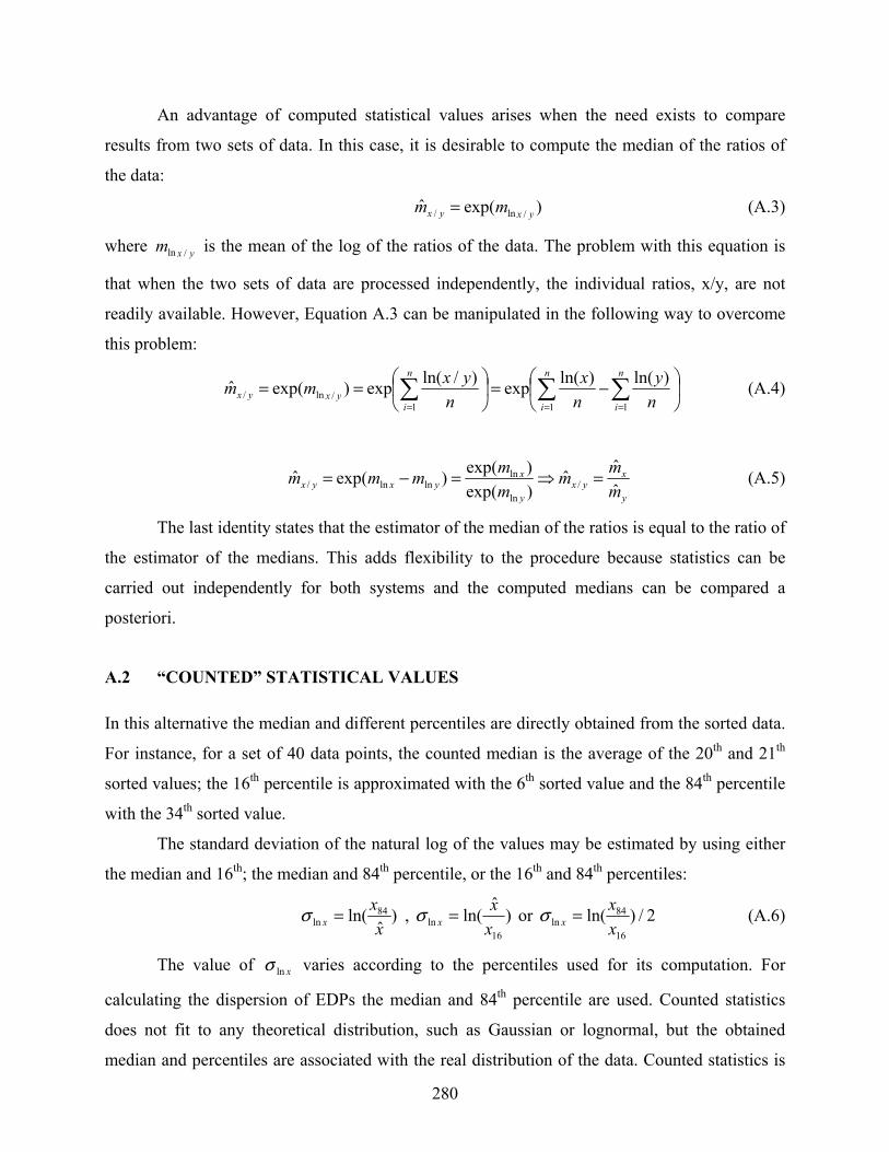
280

An advantage of computed statistical values arises when the need exists to compare

results from two sets of data. In this case, it is desirable to compute the median of the ratios of

the data:

)exp(ˆ /ln/ yxyx mm = (A.3)

where yxm /ln is the mean of the log of the ratios of the data. The problem with this equation is

that when the two sets of data are processed independently, the individual ratios, x/y, are not

readily available. However, Equation A.3 can be manipulated in the following way to overcome

this problem:

⎟⎠

⎞⎜⎝

⎛ −=⎟⎠

⎞⎜⎝

⎛== ∑∑∑===

n

i

n

i

n

iyxyx n

ynx

nyxmm

111/ln/

)ln()ln(exp)/ln(exp)exp(ˆ (A.4)

y

xyx

y

xyxyx m

mmmmmmm

ˆˆˆ

)exp()exp()exp(ˆ /

ln

lnlnln/ =⇒=−= (A.5)

The last identity states that the estimator of the median of the ratios is equal to the ratio of

the estimator of the medians. This adds flexibility to the procedure because statistics can be

carried out independently for both systems and the computed medians can be compared a

posteriori.

A.2 “COUNTED” STATISTICAL VALUES

In this alternative the median and different percentiles are directly obtained from the sorted data.

For instance, for a set of 40 data points, the counted median is the average of the 20th and 21th

sorted values; the 16th percentile is approximated with the 6th sorted value and the 84th percentile

with the 34th sorted value.

The standard deviation of the natural log of the values may be estimated by using either

the median and 16th; the median and 84th percentile, or the 16th and 84th percentiles:

)ˆ

ln( 84ln x

xx =σ , )

ˆln(

16ln x

xx =σ or 2/)ln(

16

84ln x

xx =σ (A.6)

The value of xlnσ varies according to the percentiles used for its computation. For

calculating the dispersion of EDPs the median and 84th percentile are used. Counted statistics

does not fit to any theoretical distribution, such as Gaussian or lognormal, but the obtained

median and percentiles are associated with the real distribution of the data. Counted statistics is

281

very useful when data points are missing, i.e., when EDPs are undefined because collapse has

taken place. If counted statistics is used, there is no need to stop a statistical evaluation when the

first data are missing and the process can be continued until more than 50% of the individual

data are lost.

283

Appendix B: Properties of Generic Frame Models

B.1 MODAL AND STRUCTURAL PROPERTIES OF THE GENERIC FRAMES

The main characteristics of the generic deteriorating frames used in this study are presented in

Section 5.3. These frames are based on the non-deteriorating frames developed by Medina

(2002) and have the same elastic modal and structural properties. As illustration, the modal

properties for the 9-story frames are summarized in Table B.1. The table includes participation

factors (PFi), mass participation (MPi), modal damping (ξi), and normalized mode shapes, φi.

Tables B.2 and B.3 present the following structural properties for the 9-story frames:

Stiffness properties (i denotes story or floor)

• Weight ratio, Wi/W (W = total weight)

• Moment of inertia ratio, Ii/I1 (I is the same for columns and top beam in a story)

• Story stiffness ratio (load pattern independent), Kai/Ka1. The story stiffness is defined as

the story shear force required to produce a unit displacement of a subassembly consisting

of a “story” (two columns and the beam above). The columns of the subassembly are

fixed at the base and all three elements (two columns and beam) have the same moment

of inertia.

• Floor stiffness ratio (load pattern independent), Kfi/Kf2. Floor stiffness is the story shear

force required to produce a unit displacement of a subassembly consisting of a floor beam

and half of the columns on top and below the floor level.

• Story stiffness ratio, Kki/Kk1, based upon triangular load pattern and Ksi/Ks1, based upon

parabolic load pattern. Story stiffness is defined here as the load pattern dependent story

shear force required to cause a unit story drift in that story.

• Beam stiffness ratio, Kbi/Kb2

• Spring stiffness at base, Kc = 3EI / L of the second floor beam

284

Strength and deformation parameters for a structure designed with γ = Vy / W = 1.0 and a

parabolic design load pattern without considering P-∆ effects.

• Story shear strength ratio, Vi/V1

• Story overturning moment ratio, MOT/MOT1 (overturning moment based on the axial loads

and bending moments at the bottom of the columns in a story)

• Story strain-hardening ratio from pushover analysis, αsi

• Floor beam strength ratio, Mybi/Myb2

• Column strength at base, Myc

• Beam end yield rotation ratio, θyi/θy2

• Column yield rotation at base, θyc

• Story drift ratio, δsi/δr, where δsi is the story drift in story i, and δr is the roof

displacement

• Story drift angle ratio, θsi/θr (θi is defined as δsi/hi and θr as δr/H, where hi is the story

height and H the total height)

Information on the rest of the frames can be found in Medina (2002).

B.2 STIFFNESS OF ROTATIONAL SPRINGS AT MEMBER ENDS

Each flexural member that has the potential to deform into the inelastic range is modeled by the

following subelements connected in series: plastic hinge rotational springs at member ends and

an elastic beam-column element. Therefore, the structural properties of the member are a

combination of the properties of the subelements. The rotational stiffness of the member, Kmem,

can be derived from the structural properties of the frame (Tables B.2–B.3), e.g., for beams

subjected to double curvature bending Kmem = 6EIbeam/Lbeam. The rotational stiffness, Kmem, can be

related to the stiffness of the spring, Ks, and the stiffness of the beam-column element, Kbc,

according to the following equation:

bcs

bcs

bcs

mem KKKK

KK

K+

=+

= 111

(B.1)

285

Evident choices for subelement stiffnesses appear to be either

1. Kbc = ∞, in which case Ks = Kmem, or

2. Ks = ∞, in which case Kbc = Kmem

Both options are not desirable in the context of computer analysis with the program

DRAIN-2DX, which utilizes an event-by-event solution strategy.

An infinite beam stiffness would force all deformations into the plastic hinge springs,

which would lead to the following two problems:

• The elastic spring stiffness, which has to be defined a priori, would be the same

regardless of the moment gradient in the beam or column (e.g., 6EIbeam/Lbeam, if it is

assumed that the beam deforms in double curvature). In reality, the moment gradient may

change during the time history analysis (THA), which would not be accounted for in this

model

• All damping would have to be assigned to the rotational springs at the beam ends, which

causes spurious damping moments at frame joints that are not in static equilibrium

because DRAIN-2DX’s damping formulation is based on initial member stiffnesses (see

Section B.4).

Thus, the first option is discarded.

The second option, considering an infinite spring stiffness would cause numerical

instability problems and would also make it impossible to express strain-hardening and post-

capping stiffnesses as fractions of the elastic spring stiffness. Thus, this option also had to be

discarded.

In order to avoid the problems of the second option and to minimize the problems

associated with the first option, it was decided to use an elastic spring stiffness that is “n” times

larger than the rotational stiffness of the beam-column element, Kbc, i.e.,:

bcs nKK = (B.2)

where n is a number >> 1; a value of n = 10 was used throughout this study. The stiffness of the

subelements can now be expressed as a function of the total stiffness of the member and the

multiplier n,:

membc Kn

nK 1+= mems KnK )1( += (B.3)

286

A large value on n accomplishes the following: (a) it minimizes the problems identified

in the first option because now all damping can be assigned to the elastic beam-column element

and changes in moment gradients in this subelement can be accounted for, and (b) it permits

incorporation of all backbone and cyclic deterioration characteristics in the plastic hinge

rotational spring. But the properties of these springs need to be modified because the

deterioration properties belong to the full element and not to the springs alone.

B.3 PARAMETERS FOR DETERIORATING SPRINGS

In Section B.2 the elastic stiffness of the member is related to the elastic stiffness of the

rotational springs and the beam-column element. Additional parameters must be adjusted in the

nonlinear range to reproduce the moment-rotation relationship at the end of the elements. Figure

B.1 presents the hysteretic response of a beam member, which is the combination of the

individual moment-rotations of the springs and the beam-column element. The moment-rotation

of the beam-column element remains elastic during all the THA and the nonlinear response is

entirely due to the springs. The parameters of the plastic hinge spring must be adjusted to be able

to reproduce the nonlinear moment-rotation behavior of the member.

Strain-Hardening Coefficient. The strain-hardening coefficient of the plastic hinge of

the spring ( ss,α ) must be adjusted to obtain the strain-hardening coefficient for the moment-

rotation of the member, mems,α . Because the subelements are connected in series, the increment

in rotation of the total element in the post-yielding range is the sum of the increments in rotation

of the two subelements in this interval:

bc

in

ss

inbcsmem K

MKM ∆+∆=∆+∆=∆

,

θθθ (B.4)

where inM∆ is the increment in strength developed in the inelastic range and ssK , is the stiffness

of the spring for the strain-hardening branch. The strain-hardening coefficient of the springs as a

function of mems,α is obtained by substituting Equation B.3 into Equation B.4 and by considering

that memmem

inmem K

Mα

θ ∆=∆ :

287

mems

memsss nn

n

,

,, 1

)1(α

αα

−++

= (B.5)

Note that the strain-hardening coefficient of the spring depends only on mems,α and n. For

instance, to obtain 3% strain hardening in the moment-rotation relationship at the end of the

element, the springs require a post-yield rotational spring coefficient 0028.0, =ssα (when

10=n ).

In the extreme case that n = 0, the beam-column element is rigid and memsss ,, αα = .

Post-Capping Stiffness Coefficient. The stiffness coefficient for the post-capping

branch is calculated in the same way as that of the strain-hardening branch because it also is

expressed as a fraction of the elastic stiffness of the member. For the reference frame (Section

5.3.2), the post-capping stiffness coefficient for the moment-rotation relationship at the end of

the beam is 10.0, −=memcα . If 10=n , the post-capping stiffness coefficient to be used for the

springs is 0083.0, −=scα .

Ductility Capacity of the Spring. The ductility capacity of the spring must be adjusted

to obtain the correct ductility capacity of the moment-rotation relationship at the end of the

member. By adding the deformation of the subelements in the elastic and inelastic ranges it is

possible to derive the following equation that provides the ductility capacity of the spring:

[ ] memycmemsmemycsyc n )/()1(1)/()/( , δδαδδδδ +−−= (B.6)

For the reference frames, the ductility capacity of the moment-rotation at the end of the

beam is 4)/( =memyc δδ . The ductility capacity of the spring when 10=n is 1.33)/( =syc δδ .

Parameter γ for Cyclic Deterioration. The parameter γ to be used in the springs needs

to be adjusted to simulate the correct rate of deterioration of the moment-rotation relationship of

the member. The following expression computes γs,c,k,a for the spring:

memakcssakcs n ))(1()( ,,,,,, γγ += (B.7)

This relationship is exact only for elastic-plastic models but the error is very small (less than 1%)

for the range of strain-hardening coefficients used in this work.

288

B.4 MODELING OF PLASTIC HINGES TO AVOID SPURIOUS DAMPING MOMENTS

The damping for the generic frames is based on the Rayleigh damping formulation:

oo KMC βα += (B.8)

where C is the viscous damping matrix, M is the mass matrix, Ko is the initial stiffness matrix,

and α and βo are mass and stiffness proportional factors. This formulation is implemented in the

DRAIN-2DX computer program.

An alternative viscous damping matrix is given by:

ttt KMC βα += (B.9)

where Ct is the current damping matrix, Kt is the tangent (current) stiffness matrix, and βt is the

stiffness proportional factor.

To avoid unbalance of forces during the analysis, which is based on an event-to-event

strategy, DRAIN-2DX only utilizes the constant damping matrix formulation of Equation B.8

(DRAIN-2DX, 1993). However, a constant damping matrix causes spurious damping moments

at the joints once a change of stiffness occurs in nonlinear elements that have stiffness

proportional damping based on their initial stiffness (Bernal, 1994). That is to say, although

dynamic equilibrium is satisfied, spurious damping moments cause static equilibrium to be

violated at joints.

The use of a current damping matrix was discarded because Kt in the solution of the

equation of motion may lead to a potential unbalance of forces when an event-to-event strategy

is implemented. Moreover, it is not clear how to use a tangent stiffness formulation when

nonlinear elements have a negative slope. Thus, to obtain an approximate solution that satisfies

static and dynamic equilibrium, a constant damping matrix formulation (Equation B.8) was

selected with the following conditions: (a) plastic hinging is modeled by using nonlinear

rotational springs with an initial stiffness several times larger than that of the beam-column

element and (b) zero stiffness proportional damping is assigned to the springs.

Adjustment of Damping in Subelements

Because no stiffness proportional damping is assigned to the nonlinear rotational springs, the β

(stiffness proportional) factor for the beam-column element needs to be adjusted. For 10=n , the

289

β factor must be multiplied by 1.1 to compensate for the lack of stiffness proportional damping

provided by the rotational springs.

Table B.1 Modal properties, N = 9, T1 = 0.9 and 1.8 s

Modal Properties Story/Floor Mode ShapesMode Ti / T1 PFi MPi ξi φ1 φ2 φ3 φ4 φ5

1 1.000 1.421 0.789 0.050 0/1 0.000 0.000 0.000 0.000 0.0002 0.394 0.626 0.117 0.040 1/2 0.111 0.229 -0.491 -0.624 -0.7733 0.230 -0.298 0.045 0.050 2/3 0.222 0.431 -0.809 -0.806 -0.6314 0.152 -0.226 0.022 0.068 3/4 0.333 0.579 -0.828 -0.386 0.2955 0.107 -0.165 0.012 0.094 4/5 0.444 0.645 -0.506 0.362 0.875

5/6 0.556 0.606 0.072 0.851 0.2626/7 0.667 0.437 0.686 0.558 -0.8087/8 0.778 0.119 0.982 -0.424 -0.5448/9 0.889 -0.361 0.533 -1.000 1.000

9/10 1.000 -1.000 -1.000 0.590 -0.334

Table B.2 Structural properties, N = 9, T1 = 0.9 s

Story/Floor Stiffness Properties γ = V y / W = 1.0, Parabolic Design Load PatternWi / W Ii / I1 Kai / Ka1 Kfi / Kf2 Kki / Kk1 Ksi / Ks1 Kbi / Kb2 Kc Vi / V1 MOTi / MOT1 αsi Mybi / Myb2 Myc θybi / θyb2 θcy δsi / δr θsi / θr

0/1 7316974 64920 0.0091/2 0.111 1.000 1.000 1.000 1.000 1.000 1.000 1.000 1.000 0.036 1.000 1.000 0.096 0.8612/3 0.111 0.965 0.965 0.963 0.996 0.980 0.965 0.996 0.859 0.036 0.988 1.024 0.097 0.8753/4 0.111 0.913 0.913 0.908 0.982 0.937 0.913 0.982 0.719 0.037 0.964 1.056 0.100 0.9024/5 0.111 0.836 0.836 0.829 0.951 0.872 0.836 0.951 0.581 0.038 0.919 1.098 0.104 0.9385/6 0.111 0.739 0.739 0.727 0.895 0.785 0.739 0.895 0.447 0.039 0.846 1.145 0.109 0.9816/7 0.111 0.618 0.618 0.602 0.807 0.674 0.618 0.807 0.321 0.040 0.737 1.193 0.115 1.0317/8 0.111 0.475 0.475 0.453 0.681 0.541 0.475 0.681 0.207 0.042 0.587 1.234 0.120 1.0848/9 0.111 0.311 0.311 0.275 0.509 0.385 0.311 0.509 0.112 0.043 0.388 1.247 0.126 1.138

9/10 0.111 0.131 0.131 0.500 0.284 0.206 0.131 0.284 0.040 0.045 0.147 1.120 0.132 1.189W I1 Ka1 Kf2 Kk1 Ks1 Kb2 V1 MOT1 Myb2 θyb2 δr θr

(k) (in4) (k/in) (k/in) (k/in) (k/in) (k-in) (k-in) (k) (k-in) (k-in) (k-in) (rad) (rad) (in) (rad)1800 24222 3226 562 1141 1120 14633949 1800 1841684 130200 0.009 16.800 0.013

Table B.3 Structural properties, N = 9, T1 = 1.8 s

Story/Floor Stiffness Properties γ = V y / W = 1.0, Parabolic Design Load PatternWi / W Ii / I1 Kai / Ka1 Kfi / Kf2 Kki / Kk1 Ksi / Ks1 Kbi / Kb2 Kc Vi / V1 MOTi / MOT1 αsi Mybi / Myb2 Myc θybi / θyb2 θcy δsi / δr θsi / θr

0/1 1829244 64920 0.0351/2 0.111 1.000 1.000 1.000 1.000 1.000 1.000 1.000 1.000 0.036 1.000 1.000 0.096 0.8612/3 0.111 0.965 0.965 0.963 0.996 0.980 0.965 0.996 0.859 0.036 0.988 1.024 0.097 0.8763/4 0.111 0.913 0.913 0.908 0.982 0.938 0.913 0.982 0.719 0.037 0.964 1.056 0.100 0.9024/5 0.111 0.836 0.836 0.829 0.951 0.873 0.836 0.951 0.581 0.038 0.919 1.098 0.104 0.9385/6 0.111 0.739 0.739 0.727 0.895 0.785 0.739 0.895 0.447 0.039 0.846 1.145 0.109 0.9816/7 0.111 0.618 0.618 0.602 0.807 0.674 0.618 0.807 0.321 0.040 0.737 1.193 0.115 1.0317/8 0.111 0.475 0.475 0.453 0.681 0.541 0.475 0.681 0.207 0.042 0.587 1.234 0.120 1.0848/9 0.111 0.311 0.311 0.275 0.509 0.385 0.311 0.509 0.112 0.043 0.388 1.247 0.126 1.138

9/10 0.111 0.131 0.131 0.220 0.284 0.206 0.131 0.284 0.040 0.045 0.147 1.120 0.132 1.190W I1 Ka1 Kf2 Kk1 Ks1 Kb2 V1 MOT1 Myb2 θyb2 δr θr

(k) (in4) (k/in) (k/in) (k/in) (k/in) (k-in) (k-in) (k) (k-in) (k-in) (k-in) (rad) (rad) (in) (rad)1800 6055 807 141 284 281 3658487 1800 1841684 130200 0.036 66.900 0.052

290

MOMENT-ROTATION FOR ROOF BEAM, FRAME 0303Peak Oriented Model, , NR94cnp, ξ=5%, R=3,

αs=0.03, αc=-0.10, δc/δy=4, γs,c,k,a=100

-1.5

-1

-0.5

0

0.5

1

1.5

-2 0 2 4 6 8Normalized Rotation

Nor

mal

ized

Mom

ent

SpringBeam-Col. ElementMember

Fig. B.1 Moment-rotation relationship for a member based on the moment-rotation

of the plastic hinge springs and elastic beam-column element

291

Appendix C: Probability Distribution of Collapse Capacity

In much of this report, estimators for the geometric mean and dispersion of collapse capacity are

computed without fitting a distribution to the data. However, sometimes it is more convenient to

evaluate global collapse and mean annual frequency of collapse by fitting a continuous

distribution. Information about the distribution of collapse capacities is not reported in the

literature, although it is known that the response of nonlinear structures may fit a lognormal

distribution (Shome and Cornell, 1999). Furthermore, the distribution of collapse capacity due to

RTR variability presents a long upper tail (Figs. 2.4–2.5), which suggests that a lognormal

distribution may fit well. This appendix intends to verify that a lognormal distribution can be a

good fitting of collapse capacity distribution.

C.1 LOGNORMAL DISTRIBUTION PAPER AND KOLMOGOROV-SMIRNOV GOODNESS-OF-FIT TEST

A widespread method for verifying the distribution assumption is to plot the results in a

probability paper to obtain a straight line for the assumed distribution. If the assumption is

reasonable, the cumulative frequency curve of the data is close to the straight line, and shows no

systematic curvature.

A Kolmogorov-Smirnov goodness of-fit-test is used to quantify how well the data fit the

distribution models. The tests concentrates on the deviation between the hypothesized

cumulative distribution function, )(xFX , and the observed cumulative histogram (Benjamin and

Cornell, 1970):

niXF i =)(* )( (C.1)

292

in which )(iX is the ith largest observed value in the random sample of size n. The maximum of

the aforementioned deviations is calculated as follows,

[ ])()(*max )()(

1

iX

in

iXFXFD −=

= (C.2)

That is to say, D is the largest of the absolute values of the n differences between the

hypothesized CDF and the observed empirical CDF (counted) evaluated at the observed values

in the sample. Theoretically, the value of D depends on n. For a specified significance level α,

the test compares the observed maximum difference D with the critical value c, as follows:

α−=≤ 1][ cDP (C.3)

Critical values c at various significance levels α are tabulated in Benjamin and Cornell

(1970). If the observed D is less than the critical value c, the proposed distribution is accepted at

the specified significance level α; otherwise, the assumed distribution would be rejected.

C.2 COLLAPSE CAPACITY DISTRIBUTION DUE TO RTR VARIABILITY

In this section goodness-of-fit tests are illustrated for a lognormal distribution that is fitted to

collapse capacity data in which the dispersion is entirely due to RTR variability. Collapse

capacities for three different peak-oriented SDOF systems, with T = 0.6 s, are plotted on

lognormal probability paper along with the fitted lognormal distribution (Fig. C.1). The left

vertical axis corresponds to the inverse function for the standard normal distribution of the CDF

of collapse capacity, ]}/)/[({ ,1 ηgSF ca

−Φ or in a simplified way }{,,

1

caSCF−Φ . The right vertical

axis indicates the corresponding cumulative probabilities. The graphs are for systems with “low,”

“intermediate,” and “high” ductility and the data fit well to a straight line, even at small and large

fractiles.

For this evaluation, the 5% significance level is selected, which is of common use. The

number of collapse capacities is 40, which is the number of ground motions in the LMSR-N set

to which the system is subjected. For a set of 40 data points and a 5% significant level (α =

0.05), the critical value is c = 0.21 26(Benjamin and Cornell, 1970). The test statistic (D) is

included in Figures C.1–C.3 for the three aforementioned SDOF systems. Because the test

26 For a sample size with a number of data, n, larger than 40, the critical statistic at 5% confidence level can be computed as nc /36.1=

293

statistic values are less than the critical value, the assumption of lognormal distribution for

collapse capacity cannot be rejected at the 5% significance level.

Figure C.2 shows lognormal distribution fittings for collapse capacities generated for 3

and 6-story generic frames that have a fundamental period T1 = 0.6 s. The dispersion of the data

is also entirely due to RTR variability. Once again, the visual fit is satisfactory and the computed

“D” are smaller than c = 0.21. Thus, the assumption of lognormal distribution for collapse

capacities of these generic frames cannot be rejected at the 5% significance level.

C.3 SUMMARY

The collapse capacities of several systems were plotted on lognormal probability paper along

with the fitted lognormal distribution, obtaining a good fit even at small and large fractiles. To

quantify how well the collapse capacity data fit the lognormal distribution, Kolmogorow-

Smirnov goodness-of-fit tests have been carried out. SDOF systems with low, intermediate and

high ductile characteristics, as well as stiff and flexible generic frames have been tested. In all

cases the critical value “c” for a 5% significance level is almost twice as large as the computed

parameter D. These tests provide good arguments for representing collapse capacity data by a

lognormal distribution.

294

Collapse Capacities on Lognormal Probability Paper,T = 0.6 s., Peak Oriented Model, LMSR-N, ξ=5%, P-∆='0.1N',


-2

-1.5

-1

-0.5

0

0.5

1

1.5

2

0 0.2 0.4 0.6 0.8 1 1.2 1.4 1.6log[(Sa,c/g)/η]

Φ-1

{F[(S

a,c/g

)/ η]}

D = 0.118 < c = 0.21

0.98

0.16

0.50

0.84

0.02

RTR Variability



-2

-1.5

-1

-0.5

0

0.5

1

1.5

2

0 0.2 0.4 0.6 0.8 1 1.2 1.4 1.6log[(Sa,c/g)/η]

Φ-1

{F[(S

a,c/g

)/ η]}

D = 0.127 < c = 0.21

0.98

0.16

0.50

0.84

0.02

RTR Variability

(a) High Ductility (b) Intermediate Ductility



-2

-1.5

-1

-0.5

0

0.5

1

1.5

2

0 0.2 0.4 0.6 0.8 1 1.2 1.4 1.6log[(Sa,c/g)/η]

Φ-1

{F[(S

a,c/g

)/ η]}

D = 0.126 < c = 0.21

0.98

0.16

0.50

0.84

0.02

RTR Variability

(c ) Low Ductility

Fig. C.1 Fitting of lognormal distribution to collapse capacity data; peak-oriented

SDOF systems; dispersion due to RTR variability

Collapse Capacities on Lognormal Probability Paper,

N=3, T = 0.6 s., BH, Peak Oriented Model, LMSR-N, ξ=5%αs=0.03, αc=-0.10, δc/δy=4, γs,c,a=Inf, γk=Inf, λ=0

-2

-1.5

-1

-0.5

0

0.5

1

1.5

2

0 0.2 0.4 0.6 0.8 1 1.2 1.4 1.6log[(Sa,c/g)/η]

Φ-1

{F[(S

a,c/g

)/ η]}

D = 0.129 < c = 0.21

0.98

0.16

0.50

0.84

0.02

RTR Variability

Collapse Capacities on Lognormal Probability Paper,N=6, T = 0.6 s., BH, Peak Oriented Model, LMSR-N, ξ=5%


-2

-1.5

-1

-0.5

0

0.5

1

1.5

2

0 0.2 0.4 0.6 0.8 1 1.2 1.4 1.6log[(Sa,c/g)/η]

Φ-1

{F[(S

a,c/g

)/ η]}

D = 0.117 < c = 0.21

0.98

0.16

0.50

0.84

0.02

RTR Variability

(a) 3-Story Frame (Flexible) (b) 6-Story Frame (Stiff)

Fig. C.2

Fitting of lognormal distribution to collapse capacity data; generic

frames with T1 = 0.6 s; springs with intermediate ductility

295

Appendix D: Computations of Variance of Collapse Capacity in the Linear Domain of the Data

In Chapter 6 additional variance of collapse capacity due to uncertainty in the system parameters

is computed by applying the FOSM method in the log domain of the data. As an alternative, this

appendix presents an overview of the FOSM method with computations in the linear domain of

the data. Arguments are presented for why computations in the log domain of the data are

preferable.

D.1 FORMULATION FOR COMPUTATIONS OF COLLAPSE CAPACITY IN LINEAR DOMAIN

An “additive” approach is used for computing the total variance in the linear domain of the data,

i.e., collapse capacity is expressed as a function “f” plus a random variable that depends on RTR

variability:

( )RTRQfS zca εη += )(/, (D.1)

where Q is the vector of random system parameters and ( )RTRzε is a random variable with zero

mean. Then, the total variance of collapse capacity, 2)(, TOTS ca

σ , is given by:

2)(

1 1,

2)( ,,

)()(RTRS

n

i

n

jqqqq

QjiTOTS cajiji

q

ca qQf

qQf σσσρσ

µ

+⎟⎟⎠

⎞⎜⎜⎝

⎛

∂∂

∂∂≅∑∑

= = =

(D.2)

To compare results obtained in the log and linear domain of the data, the geometric mean

and dispersion of the probabilistic parameter(s) must be equivalent. Because the distribution of

the system parameters is unknown, a first-order approximation is used:

)exp( ln xx µµ ≅ , xxx lnσµσ ≅ (D.3)

296

D.2 LINEAR DOMAIN AND LOG DOMAIN OF DATA

Some arguments in favor of the use of computations in the log domain of the data are presented

based on the reference SDOF system of Chapter 4, considering uncertainty in the post-capping

stiffness coefficient, αc. The first argument is related with the differences in the formulation, i.e.,

the multiplicative versus additive approach. The second one is about the stability in the

computations of the variance of collapse capacity.

D.2.1 Multiplicative versus Additive Approach

Computations in the log domain of the data are based on a multiplicative approach, i.e., the

random variable ( )RTRkε multiplies the function ),...,,( 21 nQQQf (Eq. 6.4). Thus, in the log

domain of the data 2)(ln , RTRS ca

σ is added to the variance of collapse capacity due to uncertainty in

the input parameters (Equation 6.8). This implies that the standard deviation of the log of

collapse capacity due to RTR variability is the same for variations of a given probabilistic

parameter ( )(ln , RTRS caσ is constant under variations of xi). In the linear domain, this means that

)(,... RTRS ca

voc is constant under variations of xi

On the other hand, the computations in the linear domain of the data consider an additive

approach, i.e., the random variable ( )RTRzε is added to the function ),...,,( 21 nQQQf . This

implies that the standard deviation of collapse capacity due to RTR variability is assumed as a

constant for variations of the probabilistic parameter ( )(, RTRS caσ is constant under variations of xi).

Figures D.1–D.2 show the behavioral trends of )(, RTRS caσ and )(,

... RTRS cavoc under

variations of αc, for reference SDOF systems at different periods. The patterns indicate that the

)(,... RTRS ca

voc tends to be more constant under variations of αc. This trend is more consistent with

the multiplicative approach. Therefore, the computations in the log domain of the data are the

most reasonable alternative from this point of view. Similar patterns were obtained for variations

of ductility capacity and cyclic deterioration.

297

D.2.2 Computations in Linear and Log Domain of Data

The additional variance of collapse capacity for the reference SDOF system due to uncertainty in

the post-capping stiffness coefficient ( 2)(, ασ

caS ) is obtained by applying the FOSM method with

computations in the linear domain of the data, (see Section 6.3.1.1). The mean and standard

deviation of cα are derived from Equation D.3: 10.0≅αµ and 06.0)6.0(10.0 =≅ασ . Once the

sign is inverted27, the 16th and 84th percentiles for computations in the linear domain of the data

are obtained:

04.006.010.016 −=+−=+≅ ααα σµth

16.006.010.084 −=−−=+≅ ααα σµth

Note that these percentiles differ from those computed in the log domain of the data for

the 16th and 84th percentiles (αc = -0.055 and -0.182, respectively). The discrepancy adds another

source of uncertainty to the comparison.

Once the collapse capacities for the 16th and 84th percentiles of cα in the linear domain of

the data are computed, 2)(, ασ

caS is calculated according to Equation D.2 and is presented in Figure

D.3 as a percentage of variance of collapse capacity due to RTR variability ( 2)(

2)( ,,/ RTRSS cacaσσ α ).

As observed, these ratios are more than two times larger than the 2)(ln

2)(ln ,,/ RTRSS cacaσσ α ratios for

computations in the log domain of the data.

The large difference in the results of Figure D.3 may be caused by the domain of the

calculations itself or by the fact that the 16th and 84th percentiles are different for each domain. A

closer look at the region where αc is evaluated reveals that th16α is on the border of a highly

nonlinear region (Fig. D.4). To eliminate the uncertainty due to collapse capacities evaluated at

different percentiles, the 16th and 84th percentiles used for the computations in the log domain of

the data are also used for the computations in the linear domain, i.e., 055.01, −=cα and

182.02, −=cα . Note that in the linear domain these values do not correspond to the 16th and 84th

and are not at the same distance from the mean value. Figure D.5 presents the ratios of variance

of collapse capacity due to uncertainty in cα over the variance of collapse capacity due to RTR 27 The sign is inverted to be able to obtain natural logarithms (Section 6.3.1.1)

298

variability for computations on both domains. This time the ratios of additional uncertainty are

very similar. This suggests that the different formulation utilized in each domain (multiplicative

versus additive approach) is less important than the values at which the probabilistic parameter is

evaluated for obtaining the derivative.

To verify the importance of the selected percentiles of αc, the collapse capacity in the log

domain of the data is computed using the αc values that were obtained for the 16th and 84th

percentiles in the linear domain. The 2)(ln

2)(ln ,,/ RTRSS cacaσσ α ratios for different percentiles in the

log domain of the data are very similar (Fig. D.6). This indicates that the dependence of collapse

capacity on the selected percentiles of αc is less sensitive in the log domain of the data (Fig. 6.4).

D.3 SUMMARY

The above observations for uncertainty in the post-capping stiffness coefficient were also made

for uncertainty in ductility capacity and cyclic deterioration. Thus, computations in the log

domain of the data should be preferred for several reasons. In the first place, the multiplicative

approach is more consistent with the identified behavioral trends of collapse capacity under

variations of the probabilistic parameter. Also, the relationships between probabilistic parameters

and collapse capacities are smoother in the log domain of the data, which tends to reduce

variations in the results due to local irregularities. However, the main reason for this preference

is that computations in the log domain of the data reduce the likelihood of evaluating collapse

capacity in a highly nonlinear region.

299

ST. DEV. OF (Sa,c/g)/η, αc VARIATIONPeak Oriented Model, LMSR-N, ξ=5%, P-∆=0, αs=0.03, αc=Var, δc/δy=4, γs,c,a=100, γk=200, λ=0

0

2

4

6

8

0 5 10 15 20 25Median (Sa,c/g)/η

st. d

ev. o

f (S a

,c/g

)/ η

T=0.3T=0.6T=0.9T=1.8T=3.6−αc = 0.04, 0.06, 0.07, 0.09, 0.10, 0.12, 0.14, 0.18, 0.25

Fig. D.1 Standard deviation of collapse capacity under variations of αc

C.O.V. OF (Sa,c/g)/η, αc VARIATIONPeak Oriented Model, LMSR-N, ξ=5%, P-∆=0, αs=0.03, αc=Var, δc/δy=4, γs,c,a=100, γk=200, λ=0

0

0.1

0.2

0.3

0.4

0.5

0.6

0 5 10 15 20 25Median (Sa,c/g)/η

c.o.

v. d

ev. o

f (S a

,c/g

)/ η

T=0.3T=0.6T=0.9T=1.8T=3.6−αc = 0.04, 0.06, 0.07, 0.09, 0.10, 0.12, 0.14, 0.18, 0.25

Fig. D.2 Coefficient of variation of collapse capacity under variations of αc

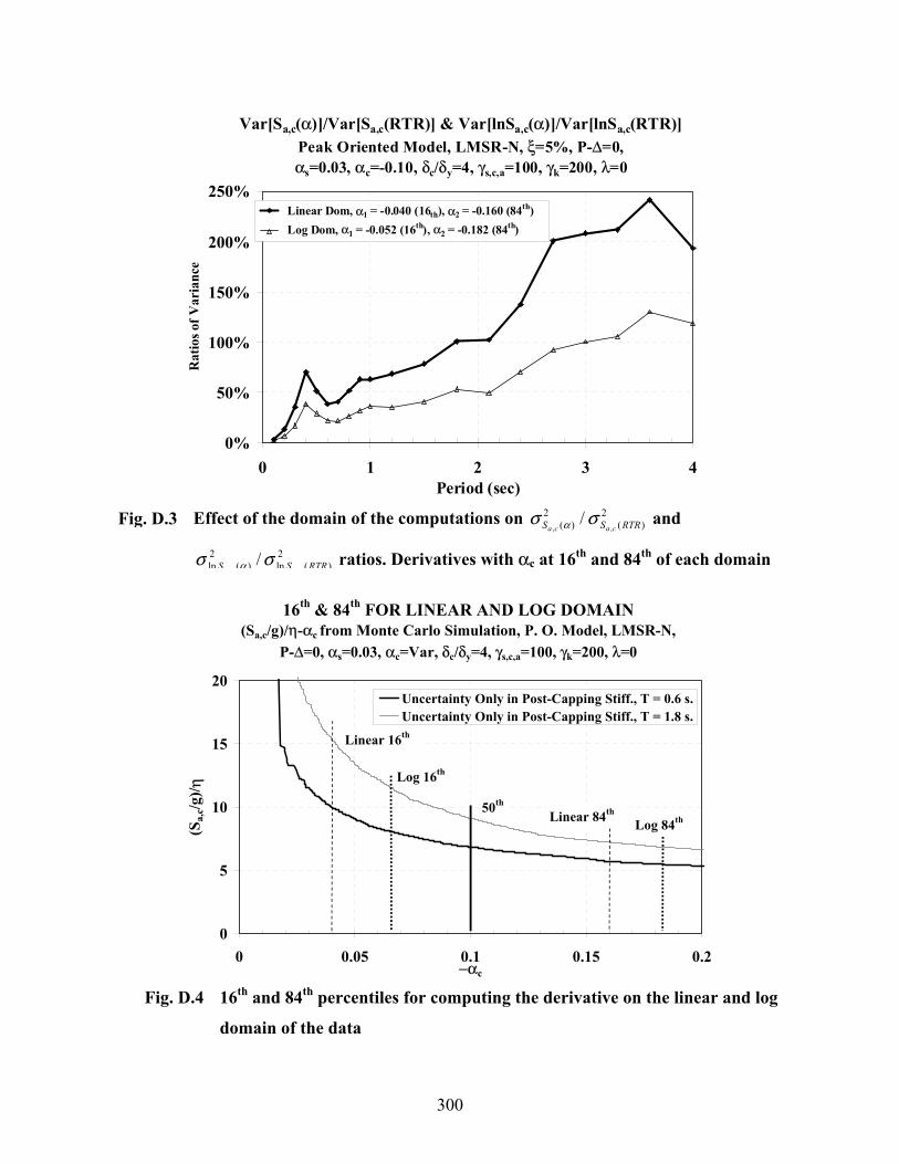
300

Var[Sa,c(α)]/Var[Sa,c(RTR)] & Var[lnSa,c(α)]/Var[lnSa,c(RTR)]Peak Oriented Model, LMSR-N, ξ=5%, P-∆=0, αs=0.03, αc=-0.10, δc/δy=4, γs,c,a=100, γk=200, λ=0

0%

50%

100%

150%

200%

250%


Rat

ios o

f Var

ianc

eLinear Dom, α1 = -0.040 (16th), α2 = -0.160 (84th)Log Dom, α1 = -0.052 (16th), α2 = -0.182 (84th)

Fig. D.3

Effect of the domain of the computations on 2

)(2

)( ,,/ RTRSS cacaσσ α and

2)(ln

2)(ln / RTRSS σσ α ratios. Derivatives with αc at 16th and 84th of each domain

16th & 84th FOR LINEAR AND LOG DOMAIN(Sa,c/g)/η-αc from Monte Carlo Simulation, P. O. Model, LMSR-N,

P-∆=0, αs=0.03, αc=Var, δc/δy=4, γs,c,a=100, γk=200, λ=0

0

5

10

15

20

0 0.05 0.1 0.15 0.2−αc

(Sa,

c/g)/ η

Uncertainty Only in Post-Capping Stiff., T = 0.6 s.Uncertainty Only in Post-Capping Stiff., T = 1.8 s.

50th

Log 84th

Log 16th

Linear 16th

Linear 84th

Fig. D.4

16th and 84th percentiles for computing the derivative on the linear and log

domain of the data

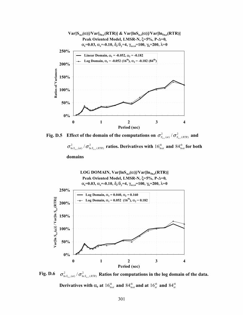
301

Var[Sa,c(α)]/Var[Sa,c(RTR)] & Var[lnSa,c(α)]/Var[lnSa,c(RTR)]Peak Oriented Model, LMSR-N, ξ=5%, P-∆=0,αs=0.03, αc=-0.10, δc/δy=4, γs,c,a=100, γk=200, λ=0

0%

50%

100%

150%

200%

250%


Rat

ios o

f Var

ianc

esLinear Domain, α1 = -0.052, α2 = -0.182 Log Domain, α1 = -0.052 (16th), α2 = -0.182 (84th)

Fig. D.5

Effect of the domain of the computations on 2)(


2)(ln

2)(ln ,,/ RTRSS cacaσσ α ratios. Derivatives with th

αln16 and thαln84 for both

domains

LOG DOMAIN, Var[lnSa,c(α)]/Var[lnSa,c(RTR)]

Peak Oriented Model, LMSR-N, ξ=5%, P-∆=0,αs=0.03, αc=-0.10, δc/δy=4, γs,c,a=100, γk=200, λ=0

0%

50%

100%

150%

200%

250%


Var

[ln S

a,c( α

)] /

Var

[ln S

a,c(

RT

R)]

Log Domain, α1 = 0.040, α2 = 0.160Log Domain, α1 = 0.052 (16th), α2 = 0.182

Fig. D.6 2

)(ln2

)(ln ,,/ RTRSS cacaσσ α Ratios for computations in the log domain of the data.

Derivatives with αc at thαln16 and th

αln84 and at thα16 and th

α84

PEER REPORTS

PEER reports are available from the National Information Service for Earthquake Engineering (NISEE). To order PEER reports, please contact the Pacific Earthquake Engineering Research Center, 1301 South 46th Street, Richmond, California 94804-4698. Tel.: (510) 231-9468; Fax: (510) 231-9 461. PEER 2005/06 Global Collapse of Frame Structures under Seismic Excitations. Luis F. Ibarra and Helmut Krawinkler.

September 2005. PEER 2005/01 Empirical Characterization of Site Conditions on Strong Ground Motion. Jonathan P. Stewart, Yoojoong Choi,

and Robert W. Graves. June 2005. PEER 2004/09 Electrical Substation Equipment Interaction: Experimental Rigid Conductor Studies. Christopher Stearns and

André Filiatrault. February 2005. PEER 2004/08 Seismic Qualification and Fragility Testing of Line Break 550-kV Disconnect Switches. Shakhzod M. Takhirov,

Gregory L. Fenves, and Eric Fujisaki. January 2005. PEER 2004/07 Ground Motions for Earthquake Simulator Qualification of Electrical Substation Equipment. Shakhzod M.

Takhirov, Gregory L. Fenves, Eric Fujisaki, and Don Clyde. January 2005. PEER 2004/06 Performance-Based Regulation and Regulatory Regimes. Peter J. May and Chris Koski. September 2004.

PEER 2004/05 Performance-Based Seismic Design Concepts and Implementation: Proceedings of an International Workshop.

Peter Fajfar and Helmut Krawinkler, editors. September 2004. PEER 2004/04 Seismic Performance of an Instrumented Tilt-up Wall Building. James C. Anderson and Vitelmo V. Bertero. July

2004. PEER 2004/03 Evaluation and Application of Concrete Tilt-up Assessment Methodologies. Timothy Graf and James O. Malley.

October 2004. PEER 2004/02 Analytical Investigations of New Methods for Reducing Residual Displacements of Reinforced Concrete Bridge

Columns. Junichi Sakai and Stephen A. Mahin. August 2004. PEER 2004/01 Seismic Performance of Masonry Buildings and Design Implications. Kerri Anne Taeko Tokoro, James C.

Anderson, and Vitelmo V. Bertero. February 2004. PEER 2003/18 Performance Models for Flexural Damage in Reinforced Concrete Columns. Michael Berry and Marc Eberhard.

August 2003. PEER 2003/17 Predicting Earthquake Damage in Older Reinforced Concrete Beam-Column Joints. Catherine Pagni and Laura

Lowes. October 2004. PEER 2003/16 Seismic Demands for Performance-Based Design of Bridges. Kevin Mackie and Božidar Stojadinovi . August

2003. PEER 2003/15 Seismic Demands for Nondeteriorating Frame Structures and Their Dependence on Ground Motions. Ricardo

Antonio Medina and Helmut Krawinkler. May 2004. PEER 2003/14 Finite Element Reliability and Sensitivity Methods for Performance-Based Earthquake Engineering. Terje

Haukaas and Armen Der Kiureghian. April 2004. PEER 2003/13 Effects of Connection Hysteretic Degradation on the Seismic Behavior of Steel Moment-Resisting Frames. Janise

E. Rodgers and Stephen A. Mahin. March 2004. PEER 2003/12 Implementation Manual for the Seismic Protection of Laboratory Contents: Format and Case Studies. William T.

Holmes and Mary C. Comerio. October 2003. PEER 2003/11 Fifth U.S.-Japan Workshop on Performance-Based Earthquake Engineering Methodology for Reinforced

Concrete Building Structures. February 2004. PEER 2003/10 A Beam-Column Joint Model for Simulating the Earthquake Response of Reinforced Concrete Frames. Laura N.

Lowes, Nilanjan Mitra, and Arash Altoontash. February 2004. PEER 2003/09 Sequencing Repairs after an Earthquake: An Economic Approach. Marco Casari and Simon J. Wilkie. April 2004.

PEER 2003/08 A Technical Framework for Probability-Based Demand and Capacity Factor Design (DCFD) Seismic Formats. Fatemeh Jalayer and C. Allin Cornell. November 2003.

PEER 2003/07 Uncertainty Specification and Propagation for Loss Estimation Using FOSM Methods. Jack W. Baker and C. Allin

Cornell. September 2003. PEER 2003/06 Performance of Circular Reinforced Concrete Bridge Columns under Bidirectional Earthquake Loading. Mahmoud

M. Hachem, Stephen A. Mahin, and Jack P. Moehle. February 2003. PEER 2003/05 Response Assessment for Building-Specific Loss Estimation. Eduardo Miranda and Shahram Taghavi.

September 2003. PEER 2003/04 Experimental Assessment of Columns with Short Lap Splices Subjected to Cyclic Loads. Murat Melek, John W.

Wallace, and Joel Conte. April 2003. PEER 2003/03 Probabilistic Response Assessment for Building-Specific Loss Estimation. Eduardo Miranda and Hesameddin

Aslani. September 2003. PEER 2003/02 Software Framework for Collaborative Development of Nonlinear Dynamic Analysis Program. Jun Peng and

Kincho H. Law. September 2003. PEER 2003/01 Shake Table Tests and Analytical Studies on the Gravity Load Collapse of Reinforced Concrete Frames. Kenneth

John Elwood and Jack P. Moehle. November 2003. PEER 2002/24 Performance of Beam to Column Bridge Joints Subjected to a Large Velocity Pulse. Natalie Gibson, André

Filiatrault, and Scott A. Ashford. April 2002. PEER 2002/23 Effects of Large Velocity Pulses on Reinforced Concrete Bridge Columns. Greg L. Orozco and Scott A. Ashford.

April 2002. PEER 2002/22 Characterization of Large Velocity Pulses for Laboratory Testing. Kenneth E. Cox and Scott A. Ashford. April

2002. PEER 2002/21 Fourth U.S.-Japan Workshop on Performance-Based Earthquake Engineering Methodology for Reinforced

Concrete Building Structures. December 2002. PEER 2002/20 Barriers to Adoption and Implementation of PBEE Innovations. Peter J. May. August 2002. PEER 2002/19 Economic-Engineered Integrated Models for Earthquakes: Socioeconomic Impacts. Peter Gordon, James E.

Moore II, and Harry W. Richardson. July 2002. PEER 2002/18 Assessment of Reinforced Concrete Building Exterior Joints with Substandard Details. Chris P. Pantelides, Jon

Hansen, Justin Nadauld, and Lawrence D. Reaveley. May 2002. PEER 2002/17 Structural Characterization and Seismic Response Analysis of a Highway Overcrossing Equipped with

Elastomeric Bearings and Fluid Dampers: A Case Study. Nicos Makris and Jian Zhang. November 2002. PEER 2002/16 Estimation of Uncertainty in Geotechnical Properties for Performance-Based Earthquake Engineering. Allen L.

Jones, Steven L. Kramer, and Pedro Arduino. December 2002. PEER 2002/15 Seismic Behavior of Bridge Columns Subjected to Various Loading Patterns. Asadollah Esmaeily-Gh. and Yan

Xiao. December 2002. PEER 2002/14 Inelastic Seismic Response of Extended Pile Shaft Supported Bridge Structures. T.C. Hutchinson, R.W.

Boulanger, Y.H. Chai, and I.M. Idriss. December 2002. PEER 2002/13 Probabilistic Models and Fragility Estimates for Bridge Components and Systems. Paolo Gardoni, Armen Der

Kiureghian, and Khalid M. Mosalam. June 2002. PEER 2002/12 Effects of Fault Dip and Slip Rake on Near-Source Ground Motions: Why Chi-Chi Was a Relatively Mild M7.6

Earthquake. Brad T. Aagaard, John F. Hall, and Thomas H. Heaton. December 2002. PEER 2002/11 Analytical and Experimental Study of Fiber-Reinforced Strip Isolators. James M. Kelly and Shakhzod M. Takhirov.

September 2002. PEER 2002/10 Centrifuge Modeling of Settlement and Lateral Spreading with Comparisons to Numerical Analyses. Sivapalan

Gajan and Bruce L. Kutter. January 2003. PEER 2002/09 Documentation and Analysis of Field Case Histories of Seismic Compression during the 1994 Northridge,

California, Earthquake. Jonathan P. Stewart, Patrick M. Smith, Daniel H. Whang, and Jonathan D. Bray. October 2002.

PEER 2002/08 Component Testing, Stability Analysis and Characterization of Buckling-Restrained Unbonded BracesTM.

Cameron Black, Nicos Makris, and Ian Aiken. September 2002. PEER 2002/07 Seismic Performance of Pile-Wharf Connections. Charles W. Roeder, Robert Graff, Jennifer Soderstrom, and Jun

Han Yoo. December 2001. PEER 2002/06 The Use of Benefit-Cost Analysis for Evaluation of Performance-Based Earthquake Engineering Decisions.

Richard O. Zerbe and Anthony Falit-Baiamonte. September 2001. PEER 2002/05 Guidelines, Specifications, and Seismic Performance Characterization of Nonstructural Building Components and

Equipment. André Filiatrault, Constantin Christopoulos, and Christopher Stearns. September 2001. PEER 2002/04 Consortium of Organizations for Strong-Motion Observation Systems and the Pacific Earthquake Engineering

Research Center Lifelines Program: Invited Workshop on Archiving and Web Dissemination of Geotechnical Data, 4–5 October 2001. September 2002.

PEER 2002/03 Investigation of Sensitivity of Building Loss Estimates to Major Uncertain Variables for the Van Nuys Testbed.

Keith A. Porter, James L. Beck, and Rustem V. Shaikhutdinov. August 2002. PEER 2002/02 The Third U.S.-Japan Workshop on Performance-Based Earthquake Engineering Methodology for Reinforced

Concrete Building Structures. July 2002. PEER 2002/01 Nonstructural Loss Estimation: The UC Berkeley Case Study. Mary C. Comerio and John C. Stallmeyer.

December 2001. PEER 2001/16 Statistics of SDF-System Estimate of Roof Displacement for Pushover Analysis of Buildings. Anil K. Chopra,

Rakesh K. Goel, and Chatpan Chintanapakdee. December 2001. PEER 2001/15 Damage to Bridges during the 2001 Nisqually Earthquake. R. Tyler Ranf, Marc O. Eberhard, and Michael P.

Berry. November 2001. PEER 2001/14 Rocking Response of Equipment Anchored to a Base Foundation. Nicos Makris and Cameron J. Black.

September 2001. PEER 2001/13 Modeling Soil Liquefaction Hazards for Performance-Based Earthquake Engineering. Steven L. Kramer and

Ahmed-W. Elgamal. February 2001. PEER 2001/12 Development of Geotechnical Capabilities in OpenSees. Boris Jeremi . September 2001. PEER 2001/11 Analytical and Experimental Study of Fiber-Reinforced Elastomeric Isolators. James M. Kelly and Shakhzod M.

Takhirov. September 2001. PEER 2001/10 Amplification Factors for Spectral Acceleration in Active Regions. Jonathan P. Stewart, Andrew H. Liu, Yoojoong

Choi, and Mehmet B. Baturay. December 2001. PEER 2001/09 Ground Motion Evaluation Procedures for Performance-Based Design. Jonathan P. Stewart, Shyh-Jeng Chiou,

Jonathan D. Bray, Robert W. Graves, Paul G. Somerville, and Norman A. Abrahamson. September 2001. PEER 2001/08 Experimental and Computational Evaluation of Reinforced Concrete Bridge Beam-Column Connections for

Seismic Performance. Clay J. Naito, Jack P. Moehle, and Khalid M. Mosalam. November 2001. PEER 2001/07 The Rocking Spectrum and the Shortcomings of Design Guidelines. Nicos Makris and Dimitrios Konstantinidis.

August 2001. PEER 2001/06 Development of an Electrical Substation Equipment Performance Database for Evaluation of Equipment

Fragilities. Thalia Agnanos. April 1999. PEER 2001/05 Stiffness Analysis of Fiber-Reinforced Elastomeric Isolators. Hsiang-Chuan Tsai and James M. Kelly. May 2001. PEER 2001/04 Organizational and Societal Considerations for Performance-Based Earthquake Engineering. Peter J. May. April

2001. PEER 2001/03 A Modal Pushover Analysis Procedure to Estimate Seismic Demands for Buildings: Theory and Preliminary

Evaluation. Anil K. Chopra and Rakesh K. Goel. January 2001. PEER 2001/02 Seismic Response Analysis of Highway Overcrossings Including Soil-Structure Interaction. Jian Zhang and Nicos

Makris. March 2001.

PEER 2001/01 Experimental Study of Large Seismic Steel Beam-to-Column Connections. Egor P. Popov and Shakhzod M. Takhirov. November 2000.

PEER 2000/10 The Second U.S.-Japan Workshop on Performance-Based Earthquake Engineering Methodology for Reinforced

Concrete Building Structures. March 2000. PEER 2000/09 Structural Engineering Reconnaissance of the August 17, 1999 Earthquake: Kocaeli (Izmit), Turkey. Halil Sezen,

Kenneth J. Elwood, Andrew S. Whittaker, Khalid Mosalam, John J. Wallace, and John F. Stanton. December 2000.

PEER 2000/08 Behavior of Reinforced Concrete Bridge Columns Having Varying Aspect Ratios and Varying Lengths of

Confinement. Anthony J. Calderone, Dawn E. Lehman, and Jack P. Moehle. January 2001. PEER 2000/07 Cover-Plate and Flange-Plate Reinforced Steel Moment-Resisting Connections. Taejin Kim, Andrew S. Whittaker,

Amir S. Gilani, Vitelmo V. Bertero, and Shakhzod M. Takhirov. September 2000. PEER 2000/06 Seismic Evaluation and Analysis of 230-kV Disconnect Switches. Amir S. J. Gilani, Andrew S. Whittaker, Gregory

L. Fenves, Chun-Hao Chen, Henry Ho, and Eric Fujisaki. July 2000. PEER 2000/05 Performance-Based Evaluation of Exterior Reinforced Concrete Building Joints for Seismic Excitation. Chandra

Clyde, Chris P. Pantelides, and Lawrence D. Reaveley. July 2000. PEER 2000/04 An Evaluation of Seismic Energy Demand: An Attenuation Approach. Chung-Che Chou and Chia-Ming Uang. July

1999. PEER 2000/03 Framing Earthquake Retrofitting Decisions: The Case of Hillside Homes in Los Angeles. Detlof von Winterfeldt,

Nels Roselund, and Alicia Kitsuse. March 2000. PEER 2000/02 U.S.-Japan Workshop on the Effects of Near-Field Earthquake Shaking. Andrew Whittaker, ed. July 2000. PEER 2000/01 Further Studies on Seismic Interaction in Interconnected Electrical Substation Equipment. Armen Der Kiureghian,

Kee-Jeung Hong, and Jerome L. Sackman. November 1999. PEER 1999/14 Seismic Evaluation and Retrofit of 230-kV Porcelain Transformer Bushings. Amir S. Gilani, Andrew S. Whittaker,

Gregory L. Fenves, and Eric Fujisaki. December 1999. PEER 1999/13 Building Vulnerability Studies: Modeling and Evaluation of Tilt-up and Steel Reinforced Concrete Buildings. John

W. Wallace, Jonathan P. Stewart, and Andrew S. Whittaker, editors. December 1999. PEER 1999/12 Rehabilitation of Nonductile RC Frame Building Using Encasement Plates and Energy-Dissipating Devices.

Mehrdad Sasani, Vitelmo V. Bertero, James C. Anderson. December 1999. PEER 1999/11 Performance Evaluation Database for Concrete Bridge Components and Systems under Simulated Seismic

Loads. Yael D. Hose and Frieder Seible. November 1999. PEER 1999/10 U.S.-Japan Workshop on Performance-Based Earthquake Engineering Methodology for Reinforced Concrete

Building Structures. December 1999. PEER 1999/09 Performance Improvement of Long Period Building Structures Subjected to Severe Pulse-Type Ground Motions.

James C. Anderson, Vitelmo V. Bertero, and Raul Bertero. October 1999. PEER 1999/08 Envelopes for Seismic Response Vectors. Charles Menun and Armen Der Kiureghian. July 1999. PEER 1999/07 Documentation of Strengths and Weaknesses of Current Computer Analysis Methods for Seismic Performance of

Reinforced Concrete Members. William F. Cofer. November 1999. PEER 1999/06 Rocking Response and Overturning of Anchored Equipment under Seismic Excitations. Nicos Makris and Jian

Zhang. November 1999. PEER 1999/05 Seismic Evaluation of 550 kV Porcelain Transformer Bushings. Amir S. Gilani, Andrew S. Whittaker, Gregory L.

Fenves, and Eric Fujisaki. October 1999. PEER 1999/04 Adoption and Enforcement of Earthquake Risk-Reduction Measures. Peter J. May, Raymond J. Burby, T. Jens

Feeley, and Robert Wood. PEER 1999/03 Task 3 Characterization of Site Response General Site Categories. Adrian Rodriguez-Marek, Jonathan D. Bray,

and Norman Abrahamson. February 1999. PEER 1999/02 Capacity-Demand-Diagram Methods for Estimating Seismic Deformation of Inelastic Structures: SDF Systems.

Anil K. Chopra and Rakesh Goel. April 1999.

PEER 1999/01 Interaction in Interconnected Electrical Substation Equipment Subjected to Earthquake Ground Motions. Armen

Der Kiureghian, Jerome L. Sackman, and Kee-Jeung Hong. February 1999. PEER 1998/08 Behavior and Failure Analysis of a Multiple-Frame Highway Bridge in the 1994 Northridge Earthquake. Gregory L.

Fenves and Michael Ellery. December 1998. PEER 1998/07 Empirical Evaluation of Inertial Soil-Structure Interaction Effects. Jonathan P. Stewart, Raymond B. Seed, and

Gregory L. Fenves. November 1998. PEER 1998/06 Effect of Damping Mechanisms on the Response of Seismic Isolated Structures. Nicos Makris and Shih-Po

Chang. November 1998. PEER 1998/05 Rocking Response and Overturning of Equipment under Horizontal Pulse-Type Motions. Nicos Makris and

Yiannis Roussos. October 1998. PEER 1998/04 Pacific Earthquake Engineering Research Invitational Workshop Proceedings, May 14–15, 1998: Defining the

Links between Planning, Policy Analysis, Economics and Earthquake Engineering. Mary Comerio and Peter Gordon. September 1998.

PEER 1998/03 Repair/Upgrade Procedures for Welded Beam to Column Connections. James C. Anderson and Xiaojing Duan.

May 1998. PEER 1998/02 Seismic Evaluation of 196 kV Porcelain Transformer Bushings. Amir S. Gilani, Juan W. Chavez, Gregory L.

Fenves, and Andrew S. Whittaker. May 1998. PEER 1998/01 Seismic Performance of Well-Confined Concrete Bridge Columns. Dawn E. Lehman and Jack P. Moehle.

December 2000.

Documents

RESEARCH CENTER - peer.berkeley.edu