RESEARCH ARTICLES Modelling and forecasting cotton

RESEARCH ARTICLES

CURRENT SCIENCE, VOL. 121, NO. 8, 25 OCTOBER 2021 1090

*For correspondence. (e-mail: [email protected])

Modelling and forecasting cotton production using tuned-support vector regression Amit Saha1,*, K. N. Singh2, Mrinmoy Ray2, Santosha Rathod3 and Sharani Choudhury4 1Central Sericultural Research and Training Institute, Central Silk Board, Srirampura, Mysuru 570 008, India 2ICAR-Indian Agricultural Statistics Research Institute, New Delhi 110 012, India 3ICAR-Indian Institute of Rice Research, Hyderabad 500 030, India 4ICAR-Indian Agricultural Research Institute, New Delhi 110 012, India

India is the largest producer of cotton in the world. For proper planning and designing of policies related to cotton, robust forecast of future production is utmost necessary. In this study, an effort has been made to model and forecast the cotton production of India using tuned-support vector regression (Tuned-SVR) model, and the importance of tuning has also been pointed out through this study. The Tuned-SVR performed better in both modelling and forecasting of cotton pro-duction compared to auto regressive integrated moving average and classical SVR models. Keywords: ARIMA, cotton production forecasting, SVR, time series, tuned-SVR. COTTON is cultivated in more than 100 countries in the world which indicates that cotton is suitable for cultivation in most of the countries. India, China, USA and Brazil are the world’s major cotton producing countries, accounting for nearly 60% of the world production. India is the second largest producer of cotton in the world as it produ-ced 6162 metric tonnes (MT) in 2020–21. Cotton industry opens up opportunities of direct and indirect employment generating revenue in the agricultural and industrial sec-tors, and in turn regulates the national economy to a good extent. Textiles and related exports, of which cotton con-stitutes nearly 65%, account for nearly 33% of the total foreign exchange earnings of our country which at pre-sent is around 12 billion dollars with a potential for a sig-nificant increase in the coming years. Though India is the largest producer of cotton in the world, cultivation of this crop and production have been facing an alarming situation. Some of the notable reasons for the same could be enhanced cost of cultivation, lesser minimum support price than demanded, declining sub-sidies, wrong policies at play, etc. The Government of India has, anyway, started to overcome the situation by introducing certain schemes such as ‘Technology Mission on Cotton’, with the aim of improving cotton production

and productivity by developing high-yielding varieties, enhancing cotton producers’ incomes by reducing the expense of cultivation, appropriate technology transfer for improved farm management practices, promoting the cultivation of Bt cotton hybrid, etc. Forecasting of crop production helps to reduce the risk associated with every step of food production, supply and consumption. This in turn urges the farmer community to invest a good amount of capital for farming, and is likely to ensure better flow of input and assistance from the government, if required, through which the overall socio-economic aspect can be significantly improved. The ideal properties of a good crop production forecast model are reliability, objectivity and consistency with scientific knowledge, adequacy to scales, minimum cost, simplicity, timeliness and sensitivity to extreme events. As agriculture has always been an uncertain business, reliable forecast is necessary for policy making to ensure sustainable growth. Government policies have big impact on the profit of cotton farmers. In 1951, United States Department of Agriculture crop reporting service de-clared that the estimates of cotton production would be increased by 15% of the actual production. After getting this information, dealers paid low price to the farmers for the supposed bumper crop which led to US$ 125 million loss to the farmers in revenues (US Congress (1952)). Therefore, governments have to make proper economic policies to deal with such problems and forecasting is inevitable for such policy making. It is the basis of what future action to take in order to secure a desired end. Hence, forecasting is absolutely necessary as it guides well to envisage the near future based on the previous years’ data analysed with the help of different statistical models. In time series modelling, auto regressive inte-grated moving average (ARIMA)1 is a widely used model in different real life examples. There are instances of ap-plication of ARIMA model for modelling and forecasting production and allied areas of various crops2–8. However, modelling and forecasting non-linear data goes beyond the capability of ARIMA models. Besides the non-linear pattern, data sometimes show more complex phenomenon with higher heterogeneity. In such complex situations,

RESEARCH ARTICLES


machine learning technique could be employed owing to its data-driven approach. Support vector machine (SVM) is one of the eminent supervised machine learning technique which was develo-ped by Cortes and Vapnik9 for binary classification pro-blems. In binary classification, the goal of SVM is to find out a hyperplane that best separates a dataset into two classes. After two years of SVM’s invention, support vector regression (SVR) based on the similar principles as SVM classification was developed by Vapnik et al.10 to deal with the regression problems. Being a non-parametric method, SVR does not depend on assumptions like linear regression. Another benefit of using SVR is that it per-mits the construction of non-linear model. So, SVR is not only popular for classification, but also for its modelling and prediction abilities. The performance of SVR is based upon proper selection of kernel, as there are different types of kernels which can be used for the classification and prediction purposes. Tremendous results were seen in regression and time series in some of the earlier studies11–16. Since the last decade, the application of SVR has been extended to time series modelling and forecasting in vari-ous areas such as power load forecasting13, rainfall fore-casting17, agricultural forecasting8,18,19 and wind power forecasting20. Some recent developments in SVM have been observed in earlier studies21–27. Another mechanism of SVM is the tuning of the model to get better prediction for testing datasets through optimi-zed parameter. So, proper selection of parameters is very important for SVR as it is highly sensitive to the choice of parameters. In light of the above discussion, modelling and forecasting of cotton production was carried out through ARIMA, SVR and tuned-SVR models. The main contributions of the proposed work are: (i) A tuned-SVR model was developed through optimized parameters for efficient and reliable forecasting of cotton production of India. (ii) The developed tuned-SVR model was compared with conventional ARIMA model as well as with untuned-SVR model.

Auto regressive integrated moving average

The autoregressive integrated moving average (ARIMA) model is the most popularly used statistical time series model in the area of time series analysis. The ARIMA1 model is expressed in mathematical form in the following expres-sion

1 1 2 2t t t p t px x x xα α α− − −= + +…+

1 1 2 2 ,t t t q t qε β ε β ε β ε− − −+ − − −…− (1)

or

1 1 2 2t t t p t px x x xα α α− − −− − −…−

1 1 2 2 , t t t q t qε β ε β ε β ε− − −= − − −…− (2)

or ) ,( ) (t tA x Aμ π ε= (3) The above model is known as ARIMA (p, q) model, where p is the autoregressive order, q, moving average order and α and β are the autoregressive and moving aver-age parameters respectively to be estimated. For example 1 1 1 1.ARIMA (1, 1) : t t t tx xα ε β ε− −= + − (4) To work with the time series, it should be stationary. But, stationary time series is not always available. It may be non-stationary in many cases. Differencing (d) is one of the methods to make non-stationary series into stationary series. After making stationary, ARIMA (p, q) model has to be applied for forecasting. Then, it is known as ARIMA (p, d, q) model. Therefore, ARIMA (2, 2, 1) is the model-ling through the ARIMA (2, 1) model after making sta-tionary by differencing the time series data twice. Various steps of ARIMA model to analyse and forecast of a time series are described below.

Step 1: Stationarity of the time series

One of the main assumptions of ARIMA model is statio-nary, in which mean and variance of the series are con-stant over time. The presence of stationarity in the data can be identified by statistical tests like Dickey–Fuller test, augmented Dickey–Fuller test. If the series exhibits a trend over time or seasonality, or if some other non-sta-tionary pattern exists, the series is differenced repeatedly until the time series becomes stationary.

Step 2: Identification of the model

The autocorrelation function (ACF) and partial autocorre-lation function (PACF) are used to identify the suitable ARIMA model orders. In the identification step, the order of tentative models could be obtained by looking for significant ACF and PACF.

Step 3: Estimation of model parameters

Once the model orders are identified, parameters are esti-mated using maximum likelihood estimation method by minimizing overall error or by maximizing the likelihood function.

Step 4: Diagnostic checking

The appropriate ARIMA model is selected using the smal-lest Akaike information criterion (AIC) or Schwarz–Bayesian

RESEARCH ARTICLES


criterion (SBC). AIC is given by using the subsequent equation AIC ( 2log 2 ),L m= − + (5) where m = p + q and L is the likelihood function. In the diagnostic checking step, it is necessary to check if the model assumptions about the errors are satisfied. The Ljung–Box test statistic is utilized to check autocor-relation in the residuals. It is expressed as

1 2

1

( 2) ( ) ,h

kk

Q n n n k r−

=

= + −∑ (6)

where h is the maximum lag, n the number of observa-tions and m is the number of parameters in the model. If the data are white noise, the Ljung–Box Q statistic has a chi-square distribution with (h – m) degrees of freedom. The null hypothesis assumed in the test are residuals which are white noise in nature.

Step 5: Forecasting and model performance

Finally, different criteria based on error terms are used to inspect the forecasting ability of the models utilized. The most commonly used accuracy measure whose scale depends on the scale of the data is root mean square error (RMSE). The RMSE which measures the overall perfor-mance of a model can be expressed as

( )21RMSE ,ˆn

t tt

y yn

= −∑ (7)

where yt is the actual value for time t, ˆty the expected value for time t and n is the number of observation.

Support vector machine in time series

Application of SVM in time series is generally utilized when the series shows non-stationarity and non-linearity process. A significant advantage of SVM is that it is not model dependent as well as independent of stationarity and linearity assumptions. However, it may be compu-tationally expensive during the training. The mathema-tical form of SVM is expressed by utilizing the observed data x(t) at time t{t = 0, 1, 2, 3, …, N}. The prediction function for non-linear regression is .( ) ( ( )) ,f x w x cφ= + (8)

where w dentoes the weights, c represents threshold value and φ(x) is known as kernel function.

For non-linear data, the mapping of x(t) is done in higher dimension feature space through some function which is denoted as φ(x), and eventually it is transformed into the linear process; and a linear regression will carry out in that feature space. The first and foremost objective is to find out the optimum value of w and c. In SVM, flatness of weights and minimization of errors are most important. The flatness of weights is denoted by ||w||2 which is the Eucledian norm and the minimization of error is called as empirical risk. However, the overall aim is to minimize the regularized risk which is the sum of empirical risk and half of the product of the flatness of weight and a constant term which is known as regularized constant. The regularized risk can be written as

2reg emp( ) ( ||

2) ||,R f R f wτ= + (9)

where Rreg( f ) is the regularized risk, Remp( f ) denotes the empirical risk, τ is denoted as constant which is called as regularized constant/capacity control term, and ||w||2 is the flatness of weights. The regularization constant has significant impact on a better fitting of the data and it can also be useful for the minimization of poor generalization effects. In other words, this constant deals with the problem of over-fitting which can be reduced by selection of proper constant value. The significance of kernel function in non-linear support vector machine (NLSVR) is very much important for mapping the data x(i) into higher dimension feature space φ(x(i)), in which the data becomes linear. The kernel function is generally expressed as follows ( , ) ( ), ( ) .k x x x xφ φ′ ′= ⟨ ⟩ (10) There are different types of kernel functions which can be used for classification and prediction problems. However, there is no such rule to make inference on which kernel one should use. All the kernels are used separately for the given datasets and whichever yields minimum error, can be chosen as a suitable kernel function in SVM. Kernel functions are used for the transformation of the given data into the required form. The radial basis function (RBF) is the most commonly used kernel function whose perfor-mance depends on various parameters which are to be selec-ted with proper care. A schematic representation of SVR architecture is depicted in Figure 1.

Steps in SVR algorithm

1. Preparation of training and testing datasets: Import the dataset and divide them into training and testing sets in the ratio of 90 : 10 or 80 : 20, etc.

RESEARCH ARTICLES


Figure 1. Architecture of support vector regression (SVR) algorithm.

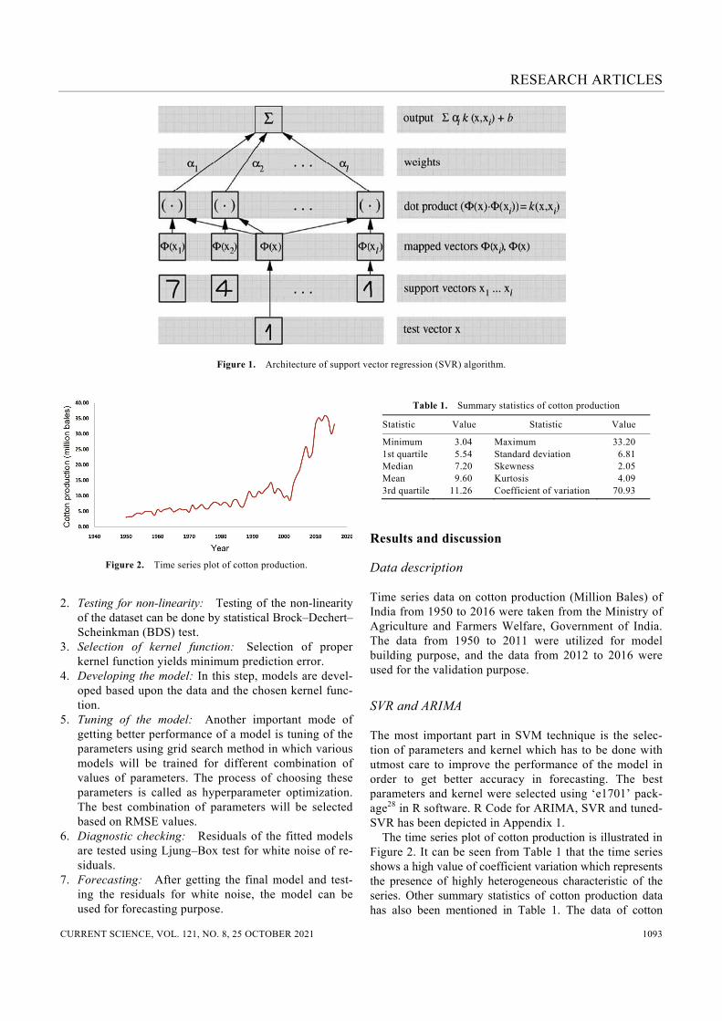
Figure 2. Time series plot of cotton production. 2. Testing for non-linearity: Testing of the non-linearity

of the dataset can be done by statistical Brock–Dechert–Scheinkman (BDS) test.

3. Selection of kernel function: Selection of proper kernel function yields minimum prediction error.

4. Developing the model: In this step, models are devel-oped based upon the data and the chosen kernel func-tion.

5. Tuning of the model: Another important mode of getting better performance of a model is tuning of the parameters using grid search method in which various models will be trained for different combination of values of parameters. The process of choosing these parameters is called as hyperparameter optimization. The best combination of parameters will be selected based on RMSE values.

6. Diagnostic checking: Residuals of the fitted models are tested using Ljung–Box test for white noise of re-siduals.

7. Forecasting: After getting the final model and test-ing the residuals for white noise, the model can be used for forecasting purpose.

Table 1. Summary statistics of cotton production

Statistic Value Statistic Value

Minimum 3.04 Maximum 33.20 1st quartile 5.54 Standard deviation 6.81 Median 7.20 Skewness 2.05 Mean 9.60 Kurtosis 4.09 3rd quartile 11.26 Coefficient of variation 70.93

Results and discussion

Data description

Time series data on cotton production (Million Bales) of India from 1950 to 2016 were taken from the Ministry of Agriculture and Farmers Welfare, Government of India. The data from 1950 to 2011 were utilized for model building purpose, and the data from 2012 to 2016 were used for the validation purpose.

SVR and ARIMA

The most important part in SVM technique is the selec-tion of parameters and kernel which has to be done with utmost care to improve the performance of the model in order to get better accuracy in forecasting. The best parameters and kernel were selected using ‘e1701’ pack-age28 in R software. R Code for ARIMA, SVR and tuned-SVR has been depicted in Appendix 1. The time series plot of cotton production is illustrated in Figure 2. It can be seen from Table 1 that the time series shows a high value of coefficient variation which represents the presence of highly heterogeneous characteristic of the series. Other summary statistics of cotton production data has also been mentioned in Table 1. The data of cotton

RESEARCH ARTICLES


Table 2. Brock–Dechert–Scheinkman test for non-linearity test of cotton production data

Embedding dimension

Statistic and P-value

Epsilon (1)

Epsilon (2)

Epsilon (3)

Epsilon (4)

m = 2 Statistic 15.74 9.40 8.45 7.04 P-value (<0.001) (<0.001) (<0.001) (<0.001) m = 3 Statistic 19.71 9.44 7.86 6.16 P-value (<0.001) (<0.001) (<0.001) (<0.001) m = 2 Statistic 25.49 9.42 7.41 5.76 P-value (<0.001) (<0.001) (<0.001) (<0.001)

Table 3. Iteration values to select best values of parameters

Epsilon Cost Error Dispersion Epsilon Cost Error Dispersion

0 4 12.27605 22.33588 0 64 27.35756 54.90826 0.1 4 12.27605 22.33588 0.1 64 27.35756 54.90826 0.2 4 12.27605 22.33588 0.2 64 27.35756 54.90826 0.3 4 12.27605 22.33588 0.3 64 27.35756 54.90826 0.4 4 12.27605 22.33588 0.4 64 27.35756 54.90826 0.5 4 12.27605 22.33588 0.5 64 27.35756 54.90826 0.6 4 12.27605 22.33588 0.6 64 27.35756 54.90826 0.7 4 12.27605 22.33588 0.7 64 27.35756 54.90826 0.8 4 12.27605 22.33588 0.8 64 27.35756 54.90826 0.9 4 12.27605 22.33588 0.9 64 27.35756 54.90826 1 4 12.27605 22.33588 1 64 27.35756 54.90826 0 8 15.34047 25.48527 0 128 42.55875 101.1322 0.1 8 15.34047 25.48527 0.1 128 42.55875 101.1322 0.2 8 15.34047 25.48527 0.2 128 42.55875 101.1322 0.3 8 15.34047 25.48527 0.3 128 42.55875 101.1322 0.4 8 15.34047 25.48527 0.4 128 42.55875 101.1322 0.5 8 15.34047 25.48527 0.5 128 42.55875 101.1322 0.6 8 15.34047 25.48527 0.6 128 42.55875 101.1322 0.7 8 15.34047 25.48527 0.7 128 42.55875 101.1322 0.8 8 15.34047 25.48527 0.8 128 42.55875 101.1322 0.9 8 15.34047 25.48527 0.9 128 42.55875 101.1322 1 8 15.34047 25.48527 1 128 42.55875 101.1322 0 16 18.08678 30.58122 0 256 71.06768 187.6855 0.1 16 18.08678 30.58122 0.1 256 71.06768 187.6855 0.2 16 18.08678 30.58122 0.2 256 71.06768 187.6855 0.3 16 18.08678 30.58122 0.3 256 71.06768 187.6855 0.4 16 18.08678 30.58122 0.4 256 71.06768 187.6855 0.5 16 18.08678 30.58122 0.5 256 71.06768 187.6855 0.6 16 18.08678 30.58122 0.6 256 71.06768 187.6855 0.7 16 18.08678 30.58122 0.7 256 71.06768 187.6855 0.8 16 18.08678 30.58122 0.8 256 71.06768 187.6855 0.9 16 18.08678 30.58122 0.9 256 71.06768 187.6855 1 16 18.08678 30.58122 1 256 71.06768 187.6855 0 32 21.68974 38.83359 0 512 75.79497 200.5918 0.1 32 21.68974 38.83359 0.1 512 75.79497 200.5918 0.2 32 21.68974 38.83359 0.2 512 75.79497 200.5918 0.3 32 21.68974 38.83359 0.3 512 75.79497 200.5918 0.4 32 21.68974 38.83359 0.4 512 75.79497 200.5918 0.5 32 21.68974 38.83359 0.5 512 75.79497 200.5918 0.6 32 21.68974 38.83359 0.6 512 75.79497 200.5918 0.7 32 21.68974 38.83359 0.7 512 75.79497 200.5918 0.8 32 21.68974 38.83359 0.8 512 75.79497 200.5918 0.9 32 21.68974 38.83359 0.9 512 75.79497 200.5918 1 32 21.68974 38.83359 1 512 75.79497 200.5918

production show the non-linearity pattern which is confir-med by the result of BDS test (Table 2). Table 2 shows the results of BDS test at embedding dimension 2, 3 and 4.

The graph in Figure 3 explains that one has to choose the values of epsilon and cost from the darkest region which will provide better model with lowest RMSE, as

RESEARCH ARTICLES


Figure 3. Plot to find out the best parameters of the SVR model.

Figure 4. Autocorrelation function plot for the cotton production data to decide the moving average order in auto regressive integrated moving average (ARIMA) model.

Figure 5. Partial autocorrelation function plot for the cotton production data to decide auto regres-sive order in ARIMA model.

RESEARCH ARTICLES


Figure 6. Graphical representation of the performance of ARIMA, SVR and tuned-SVR models.

Table 4. Parameter estimation of support vector regression

Sampling method 10-fold cross validation

Epsilon (best parameter) 0.1 Cost (best parameter) 4 Gamma (best parameter) 1 Number of support vectors 39 Best performance 12.24 SVM-type Epsilon-regression SVM-Kernel Radial basis function

Table 5. Various auto regressive integratedmoving average (ARIMA) models with their Akaike information criterion (AIC) value

Model AIC

ARIMA (2, 2, 2) 254.44 ARIMA (0, 2, 0) 288.65 ARIMA (1, 2, 0) 278.76 ARIMA (0, 2, 1) 254.84 ARIMA (1, 2, 2) Inf ARIMA (2, 2, 1) 252.07 ARIMA (1, 2, 1) 256.97 ARIMA (2, 2, 0) 259.45 ARIMA (3, 2, 1) 254.44 ARIMA (3, 2, 0) 254.83 ARIMA (3, 2, 2) 256.86

Table 6. Parameter estimation of ARIMA model

Parameters Estimate Standard error Z-value P-value

AR 1 –0.199 0.150 –1.320 0.186 AR 2 –0.435 0.149 –2.913 0.003 MA 1 –0.720 0.134 –5.348 <0.001

RMSE value is closer to zero in the darker region. Table 3 shows the iterated values for the selection of best epsilon and cost values with corresponding error and dispersion. It is not always easy to select a best parameter by visuali-zing the graph. The range of epsilon is from 0 to 1 and cost is from 4 to 512. The best parameters will be selected

from the various sets of trained models with different combinations of epsilon and cost values. Tuning of the model is very much important to get better prediction through optimized parameters. Table 4 displays the estimated optimized parameters of SVR after sufficient tuning of SVR model, and these parameters have been utilized to build the SVR model. Ten-fold cross validation is necessary as it helps to select the best parameters after using several different values and, choose those parameters which provide less RMSE. Here, ARIMA (2, 2, 1) model has been fitted based on the lowest AIC values (Table 5) among various ARIMA models which are made on the basis of ACF and PACF (Figures 4 and 5). The estimated parameters of ARIMA models are provided in Table 6. Figure 6 depicts the graphical representation of fore-casting performance of ARIMA, SVR and Tuned-SVR models. Table 7 shows the models’ performance in terms of mean square error (MSE), RMSE, mean absolute error (MAE) and mean absolute percentage error (MAPE), under training datasets for ARIMA, SVR and Tuned-SVR. The models’ performance in terms of MSE, RMSE, MAE and MAPE under testing datasets for ARIMA, SVR and Tuned-SVR is shown in Table 8. The out-of-sample fore-cast values using ARIMA, SVR and Tuned-SVR are de-picted in Table 9. It can be seen from Figure 6 that the fitted values of the Tuned-SVR model are closer to the original cotton pro-duction values, as compared to both ARIMA and SVR models both in training as well as, in testing sets. It is ob-served from Tables 8 and 9 that the tuned-SVR has a lower MSE and RMSE compared to the ARIMA and SVR models in both training and testing datasets as, one of notable features of SVR is to reduce the RMSE. In the training, SVR performed well but it failed to show good performance for unseen data. It can also be seen from Table 9 that the forecast values of the tuned-SVR are closer to the observed values compared to ARIMA and SVR models. From the above results and discussion, it can be inferred that performance of the tuned-SVR

RESEARCH ARTICLES


models is better than the ARIMA and SVR models in terms of forecasting accuracy and generalization capa-bility.

Conclusion

In reality, most of the time series data are non-linear in nature. In this study, the data of cotton production has shown non-stationary as well as non-linearity structures which were difficult to capture using ARIMA models. However, SVR has shown better performance due to its ability to capture non-linear pattern in the data, but it failed to provide better result out of the sample data. After tuning the parameters of SVR, it showed improved per-formance in both training and testing datasets as compared to ARIMA and SVR models. Based on the results, it can be inferred that tuned-SVR outperformed ARIMA and SVR models for modelling and forecasting of cotton pro-duction in India. The reported advantages of Tuned-SVR model can be extended for modelling and forecasting of other real life time series bearing non-linear pattern. Fur-ther, if the data shows mixture of linear and non-linear

Table 7. Model performance in training datasetusing ARIMA, support vector regression (SVR) and tuned-SVR

Model MSE RMSE MAE MAPE

ARIMA 6.70 2.58 1.83 12.81 SVR 5.00 2.23 0.80 6.16 Tuned-SVR 3.08 1.75 1.14 12.73

MSE, Mean square error; RMSE, Root mean squareerror; MAE, Mean absolute error; MAPE, Mean abso-lute percentage error.

Table 8. Model performance in testing dataset using ARIMA, SVR and tuned-SVR

Model MSE RMSE MAE MAPE

ARIMA 82.45 9.08 7.35 22.76 SVR 129.17 11.36 11.17 32.98 Tuned-SVR 9.48 3.07 2.54 7.83

MSE, Mean square error; RMSE, Root mean squareerror; MAE, Mean absolute error; MAPE, Mean abso-lute percentage error.

Table 9. Out-of-sample forecast values using ARIMA, SVR and tuned-SVR

Year Actual ARIMA SVR Tuned-SVR

2012 34.22 34.98 22.35 33.85 2013 35.90 38.21 22.90 34.78 2014 34.81 41.79 21.81 32.67 2015 30.00 43.82 22.60 34.33 2016 33.09 45.99 22.47 28.32

Appendix 1. R Code for ARIMA, SVR and tuned-SVR

# Install the Package “forecast and tseries” from library install.packages (“forecast”) install.packages (“tseries”) #Load Library library (forecast) library (tseries) ## Forecasting using ARIMA model #Load the data Cotton=read.table (file.choose (), header=TRUE) Head (Cotton) #Fitting of ARIMA model fit.arima=auto.arima(Cotton) fit.arima # Results of various errors accuracy(fit.arima) #Fitted values of ARIMA model fitted=fit.arima$fitted # out of sample forecast based upon the fitted model for next five years fcast=forecast(fit.arima, h=5) # Save the results in csv format write.csv(as.data.frame(fitted), file=“fitted.csv”) # Install the Package “e1071” from library install.packages (“e1071”) #Load Library library (e1071) #Load the data Cotton=read.table (file.choose (), header=TRUE) Head (Cotton) x=Cotton[,1] y=Cotton[,2] # Modelling the time series for prediction using SVR model<-svm (x, y, kernel=“linear/polynomial/radial/sigmoid”) # The results of the fitted model summary (model) # Make the prediction for each X predictedY<-predict (model, Cotton) #Display the predictions points (Cotton$x, predictedY, col=“red”,pch=4) error<-model$residuals ##Perform a grid search for tuning SVR model by varying values of parameters # Tune the SVR model tuneresult<-tune(svm,y~x,data=oil, ranges=list(epsilon=seq(0.1,0.1), cost=2^(2:9))) #Draw the tuning of graph Print (tuneresult) ## Selection of best model # Find out the best model tunemodel<-tuneresult$best.model # Predict the time series using chosen best model tunemodelY<-predict(tunemodel, Cotton) tunemodelY #Residual after fitting the model error<-Cotton$Y-tunemodelY # Save the results in csv format write.csv(as.data.frame(tunemodelY), file=“tunemodelY.csv”) #Forecasting of out of sample data r1=read.table(file.choose(),header=TRUE) # import testing data-set x1=r1 # testing dataset predsvm = predict(model, x1) predsvm predsvm = predict(tunemodel, x1) predsvm

RESEARCH ARTICLES


patterns, then a hybrid model can be developed for mod-elling and forecasting by considering unique strengths of linear and non-linear models. Conflicting interests: The author(s) declare no potential conflicts of interest with respect to the research, author-ship, and/or publication of this article.

1. Box, G. E. P. and Jenkins, G., Time series analysis, forecasting and control. Holden-Day, San Francisco, CA, 1970.

2. Ariyo, A. A., Adewumi, A. O. and Ayo, C. K., Stock price predic-tion using the ARIMA model. In UK Sim-AMSS 16th International Conference on Computer Modelling and Simulation, IEEE, 2014, pp. 106–112.

3. Badmus, M. A. and Ariyo, O. S., Forecasting cultivated areas and production of maize in Nigerian using ARIMA Model. Asian J. Agric. Sci., 2011, 3(3), 171–176.

4. Bari, S. H., Rahman, M. T., Hussain, M. M. and Ray, S., Forecast-ing monthly precipitation in Sylhet city using ARIMA model. Civil Environ. Res., 2015, 7(1), 69–77.

5. Suresh, K. K. and Priya, S. K., Forecasting sugarcane yield of Tamil Nadu using ARIMA models. Sugar Tech., 2011, 13(1), 23–26.

6. Padhan, P. C., Application of ARIMA model for forecasting agri-cultural productivity in India. J. Agric. Soc. Sci., 2012, 8(2), 50–56.

7. Prabakaran, K. and Sivapragasam, C., Forecasting areas and pro-duction of rice in India using ARIMA model. Int. J. Farm Sci., 2014, 4(1), 99–106.

8. Sarika, Iquebal, M. A. and Chattopadhyay, C., Modelling and fore-casting of pigeonpea (Cajanuscajan) production using autoregres-sive integrated moving average methodology. Indian J. Agric. Sci., 2011, 81(6), 520–523.

9. Cortes, C. and Vapnik, V., Support-vector network. Mach. Learn., 1995, 20, 1–25.

10. Vapnik, V., Golowich, S. and Smola, A., Support vector method for function approximation, regression estimation, and signal processing. In Advances in Neural Information Processing Sys-tems (eds Mozer, M., Jordan, M. and Petsche, T.), MIT Press, Cambridge, USA, 1997, vol. 9, pp. 281–287.

11. Mattera, D. and Haykin, S., Support vector machines for dynamic reconstruction of achaotic system. In Advances in Kernel Me-thods – Support Vector Learning (eds Schölkopf, B. et al.), MIT Press, Cambridge, USA, 1999, pp. 211–242.

12. Muller, K. R., Smola, A., R¨atsch, G., Schölkopf, B., Kohlmorgen, J. and Vapnik, V., Predicting time series with support vector machines. In Artificial Neural Networks (eds Gerstner, W. et al.), ICANN 1997, Lecture Notes in Computer Science, Springer, Berlin, Germany, 1997, vol. 1327, pp. 999–1004.

13. Niu, D., Wang, Y. and Wu, D. D., Power load forecasting using support vector machine and ant colony optimization. Exp. Syst. Appl., 2010, 37, 2531–2539.

14. Saha, A., Singh, K. N., Ray, M. and Rathod, S., A hybrid spatio-temporal modelling: an application to space-time rainfall forecast-ing. Theor. Appl. Climatol., 2020, 142, 1271–1282.

15. Saha, A. and Bhattacharyya, S., Artificial insemination for milk production in India: a statistical insight. Indian J. Anim. Sci., 2021, 90, 1186–1190.

16. Stitson, M., Gammerman, A., Vapnik, V., Vovk, V., Watkins, C. and Weston, J., Support vector regression with ANOVA decompo-sition kernels. In Advances in Kernel Methods – Support Vector Learning (eds Schölkopf, B., Burges, C. J. C. and Smola, A. J.), MIT Press, Cambridge, USA, 1999, pp. 285–292.

17. Ortiz-Garcia, E. G., Salcedo-Sanz, S. and Casanova-Mateom, C., Accurate precipitation prediction with support vector classifiers: a study including novel predictive variables and observational data. Atmos. Res., 2014, 139, 128–136.

18. Kumar, T. L. M. and Prajneshu, Development of hybrid models for forecasting time-series data using nonlinear SVR enhanced by PSO. J. Stat. Theory Prac., 2015, 9(4), 699–711.

19. Rathod, S., Singh, K. N., Patil, S. G., Naik, R. H., Ray, M. and Meena, V. S., Modeling and forecasting of oilseed production of India through artificial intelligence techniques. Indian J. Agric. Sci., 2018, 88(1), 22–27.

20. De Giorgi, M. G., Campilongo, S., Ficarella, A. and Congedo, P. M., Comparison between wind power rediction models based on wavelet decomposition with least-squares support vector machine (LS-SVM) and artificial neural network (ANN). Energy, 2014, 7, 5251–5272.

21. Balasundaram, S. and Gupta, D., Lagrangian support vector re-gression via unconstrained convex minimization. Neural Networks, 2014, 51, 67–79.

22. Balasundaram, S. and Gupta, D., On implicit Lagrangian twin support vector regression by Newton method. Int. J. Comput. Intel. Syst., 2014, 7(1), 50–64.

23. Balasundaram, S. and Gupta, D., Training Lagrangian twin support vector regression via unconstrained convex minimization. Knowl.-Based Syst., 2014, 59, 85–96.

24. Balasundaram, S. and Gupta, D., On optimization based extreme learning machine in primal for regression and classification by functional iterative method. Int. J. Mach. Learn. Cybernet., 2016, 7(5), 707–728.

25. Gupta, D., Richhariya, B. and Borah, P., A fuzzy twin support vector machine based on information entropy for class imbalance learning. Neural. Comput. Appl., 2019, 31(11), 7153–7164.

26. Gupta, U. and Gupta, D., An improved regularization based Lagrangian asymmetric ν-twin support vector regression using pinball loss function. Appl. Intell., 2019, 49(10), 3606–3627.

27. Hou, Q., Zhang, J., Liu, L., Wang, Y. and Jing, L., Discriminative information-based nonparallel support vector machine. Signal. Process., 2019, 162, 169–179.

28. Meyer, D. et al., Package ‘e1071’. The R Journal, 2019. ACKNOWLEDGEMENT. We acknowledge ICAR-Indian Agricul-tural Statistics Research Institute, New Delhi for providing software and other facilities for the study. Received 13 January 2020; revised accepted 4 August 2021 doi: 10.18520/cs/v121/i8/1090-1098

Documents

RESEARCH ARTICLES Modelling and forecasting cotton