Research Article Traffic Incident Clearance Time and

Research ArticleTraffic Incident Clearance Time and Arrival Time PredictionBased on Hazard Models

Yang beibei Ji,1 Rui Jiang,2 Ming Qu,2 and Edward Chung2

1 School of Management, Shanghai University, Shangda Road 99, Shanghai, China2 Smart Transport Research Centre, Queensland University of Technology, Level 8, P Block, Brisbane, QLD 4001, Australia

Correspondence should be addressed to Yang beibei Ji; [email protected]

Received 25 February 2014; Accepted 31 March 2014; Published 17 April 2014

Academic Editor: X. Zhang

Copyright © 2014 Yang beibei Ji et al. This is an open access article distributed under the Creative Commons Attribution License,which permits unrestricted use, distribution, and reproduction in any medium, provided the original work is properly cited.

Accurate prediction of incident duration is not only important information of Traffic Incident Management System, but also aneffective input for travel time prediction. In this paper, the hazard based predictionmodels are developed for both incident clearancetime and arrival time. The data are obtained from the Queensland Department of Transport and Main Roads’ STREAMS IncidentManagement System (SIMS) for one year ending in November 2010.The best fitting distributions are drawn for both clearance andarrival time for 3 types of incident: crash, stationary vehicle, and hazard.The results show that Gamma, Log-logistic, andWeibull arethe best fit for crash, stationary vehicle, and hazard incident, respectively. The obvious impact factors are given for crash clearancetime and arrival time. The quantitative influences for crash and hazard incident are presented for both clearance and arrival. Themodel accuracy is analyzed at the end.

1. Introduction

Traffic incident is considered as one of the major factorswhich cause traffic congestion and delay. At the same timetraffic incident has wide negative impact on both trafficsystem and related social activities. Many studies have beendone to predict, estimate, or try to decrease traffic durationtime just because the accurate prediction of incident timecan (1) reduce incident duration time, (2) associate TrafficIncident Management (TIM) to quickly respond to incidentto mitigate the impact of incidents (Chou [1]), and (3)

improve travel time reliability by predicting travel time whileoccurrence of incident (Tsubota et al. [2]).

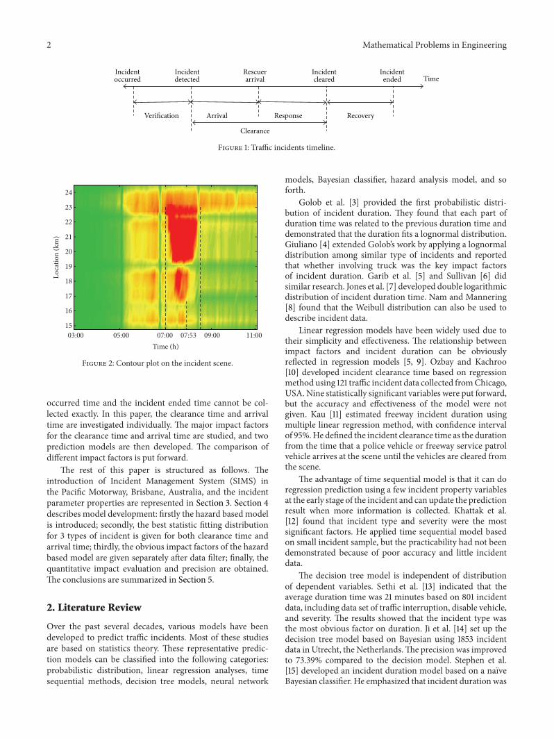
Traffic incident is nonrecurrent events which cause acapacity reduction or an abnormal increase in traffic demand,such as crash accident, stalled vehicles, debris, fire, con-struction, and sporting events. A general incident timelineas shown in Figure 1 reveals that incident duration can bedivided into verification, response, clearance, and recoveryperiod by recording timestamps at various stage of anincident.

However, most of the prediction models did not includeall four parts or did not give the exact definition of incident

time. Each part of incident time has statistic distributionand has different influence factors. An example is given inFigure 2.

Figure 2 is the occupancy contour plot from 3:00 a.m. to11:00 a.m., in which the 𝑦-axis denotes the distance from startpoint of the freeway and 𝑥-axis indicates the time. The greenindicates low occupancy (free flow conditions), the yellowindicates increasing congestion, and the red represents muchcongestion on the links. The incident is marked as the redarea where the incident occurred time (7:00 a.m.), clearedtime (7:53 a.m.), and traffic recovered time (8:20 a.m.) areclearly marked. According to the incident data base (SIMS), amultiple vehicle crash incident on 22 July in 2011 was verifiedon 7:39 a.m. and was cleared on 7:53 a.m., and the towassistance arrived on 7:47 a.m.. The total duration time was80minutes calculated based on real traffic flowdata, while theduration time was only 14 minutes according to incident database. The real duration time was almost 6 times of incidentdata base, resulting in errors of prediction model.

However, the accuracy of the incident prediction modelcannot be improved, which is partly caused by the definitionof the incident duration. It is difficult to get real incidentduration time as shown in Figure 1, because the incident

Hindawi Publishing CorporationMathematical Problems in EngineeringVolume 2014, Article ID 508039, 11 pageshttp://dx.doi.org/10.1155/2014/508039

2 Mathematical Problems in Engineering

Incident Incident Incident Incidentoccurred detected

Rescuerarrival cleared ended

Verification Arrival Response Recovery

Time

Clearance

Figure 1: Traffic incidents timeline.

03:00 05:00 07:00 07:53 09:00 11:0015

16

17

18

19

20

21

22

23

24

Time (h)

Loca

tion

(km

)

Figure 2: Contour plot on the incident scene.

occurred time and the incident ended time cannot be col-lected exactly. In this paper, the clearance time and arrivaltime are investigated individually. The major impact factorsfor the clearance time and arrival time are studied, and twoprediction models are then developed. The comparison ofdifferent impact factors is put forward.

The rest of this paper is structured as follows. Theintroduction of Incident Management System (SIMS) inthe Pacific Motorway, Brisbane, Australia, and the incidentparameter properties are represented in Section 3. Section 4describes model development: firstly the hazard based modelis introduced; secondly, the best statistic fitting distributionfor 3 types of incident is given for both clearance time andarrival time; thirdly, the obvious impact factors of the hazardbased model are given separately after data filter; finally, thequantitative impact evaluation and precision are obtained.The conclusions are summarized in Section 5.

2. Literature Review

Over the past several decades, various models have beendeveloped to predict traffic incidents. Most of these studiesare based on statistics theory. These representative predic-tion models can be classified into the following categories:probabilistic distribution, linear regression analyses, timesequential methods, decision tree models, neural network

models, Bayesian classifier, hazard analysis model, and soforth.

Golob et al. [3] provided the first probabilistic distri-bution of incident duration. They found that each part ofduration time was related to the previous duration time anddemonstrated that the duration fits a lognormal distribution.Giuliano [4] extended Golob’s work by applying a lognormaldistribution among similar type of incidents and reportedthat whether involving truck was the key impact factorsof incident duration. Garib et al. [5] and Sullivan [6] didsimilar research. Jones et al. [7] developed double logarithmicdistribution of incident duration time. Nam and Mannering[8] found that the Weibull distribution can also be used todescribe incident data.

Linear regression models have been widely used due totheir simplicity and effectiveness. The relationship betweenimpact factors and incident duration can be obviouslyreflected in regression models [5, 9]. Ozbay and Kachroo[10] developed incident clearance time based on regressionmethod using 121 traffic incident data collected fromChicago,USA. Nine statistically significant variables were put forward,but the accuracy and effectiveness of the model were notgiven. Kau [11] estimated freeway incident duration usingmultiple linear regression method, with confidence intervalof 95%.He defined the incident clearance time as the durationfrom the time that a police vehicle or freeway service patrolvehicle arrives at the scene until the vehicles are cleared fromthe scene.

The advantage of time sequential model is that it can doregression prediction using a few incident property variablesat the early stage of the incident and can update the predictionresult when more information is collected. Khattak et al.[12] found that incident type and severity were the mostsignificant factors. He applied time sequential model basedon small incident sample, but the practicability had not beendemonstrated because of poor accuracy and little incidentdata.

The decision tree model is independent of distributionof dependent variables. Sethi et al. [13] indicated that theaverage duration time was 21 minutes based on 801 incidentdata, including data set of traffic interruption, disable vehicle,and severity. The results showed that the incident type wasthe most obvious factor on duration. Ji et al. [14] set up thedecision tree model based on Bayesian using 1853 incidentdata in Utrecht, the Netherlands.The precision was improvedto 73.39% compared to the decision model. Stephen et al.[15] developed an incident duration model based on a naıveBayesian classifier. He emphasized that incident duration was

Mathematical Problems in Engineering 3

a highly variable quantity and although the model performedbetter than a linear regression, its classification was stillcorrect only in half of the time.

Artificial neural networks (ANN) have been widely usedfor prediction and pattern classification problems. Lopes etal. [16] presented an adaptive model to forecast the clearancetime of real time traffic incidents.The solutions included fourmodels which were calibrated and tested by incident recordsfrom Portuguese highways. The performance showed that itwas able to estimate 72% of incident with less than 10minuteserror and about 92% with less than 20 minutes error. Someother examples can be found in [17, 18].

The hazard analysis model has been used in trafficengineering, which is a common topic in many fields suchas life sciences, biomedical, and reliability engineering. Themodel is more effective to analyze time-related problem,which is generally used to describe the analysis of data inthe form of time from a well-defined time origin until theoccurrence of some particular event of an end point [19].Examples include the time between incident occurrence andits clearance [8, 20], the time between planning and executionof an activity [21], and the analysis of urban travel time [22].

Furthermore, hazard-based model has been used tomodel incident duration time. Chung [23] presented anaccident duration model using 2-year-accident dataset from2006 to 2007 in Korean freeway systems, and the Log-logistic distribution was selected for accelerated failure timemetricmodel. Although themodel had large prediction error,statistical test results indicated that thismodel was stable overtime. Tavassoli et al. [24] developed parametric acceleratedfailure time survival models of incident duration.They foundthat the duration of each type of incident is uniquely differentand responds to different factors.

One distinctive feature of hazard based model is thatthe model precision will be improved if the best fittingdistribution of time variable is chosen. In this study, hazardbasedmodels, in particular the accelerated failure time (AFT)metric, are utilized tomodel both incident clearance time andarrival time.

3. Description of Incident Base

Incident data was collected by Queensland Department ofTransport andMainRoads’ STREAMS IncidentManagementSystem (SIMS) for South East Queensland urban networksfromNovember 2009 to November 2010. SIMS is an incidentmanagement system which is used throughout Queensland,Australia, to capture traffic incidents which cause an impacton traffic flow on the road network. There are total 35103incident data for one year, which can be classified into 9types: alert, congestion, crash, fault, flood, hazard, plannedincident, road works, and stationary vehicles.There are manydetailed properties in SIMS incident data base, but not all ofthem are closely related to incident time prediction, such aslocation, SIMS ID, and status. Hence, the major propertiesof each incident data are shown in Table 1. However, not allthese properties are recorded for each incident occurrence.For example, the parameters are only applicable for crash data

which are “number of vehicles involved,” “number of peopleinjured,” and “number of fatalities”.

Only 3 types of incidents: crash, stationary vehicle, andhazard are used to model development though 9 types ofincident recorded in SIMS data base. Other incident typedata are rare recorded. Consequently, the clearance time andarrival time prediction model are only developed for 3 typesof incident.

4. Model Development

Hazard based time models were originally used for problemsin biomedical, engineering, and social sciences, which are aclass of statistical methods for studying the occurrence andtiming of events. Recently, they were used to model timerelated issues in transportation. A review of the applicationof the hazard based duration models in transportation up tothe early 1990s [25].

The incident time in hazard based model is a realizationof a continuous random variable 𝑇, with a cumulative distri-bution function 𝐹(𝑡), which is called the failure function. Aprobability density function 𝑓(𝑡), survival function 𝑆(𝑡), andhazard function ℎ(𝑡) are given as (2)–(4). The relationshipsbetween these four functions are formulated in (1)–(4), and𝑃(⋅) means probability. The function of a random variable 𝑇

is given by

𝐹 (𝑡) = ∫𝑡

0

𝑓 (𝑢) 𝑑𝑢 = 𝑃 (𝑇 < 𝑡) , (1)

𝑓 (𝑡) =𝑑𝐹 (𝑡)

𝑑𝑡= limΔ𝑡→0

𝑃 (𝑡 ≤ 𝑇 < 𝑡 + Δ𝑡)

Δ𝑡, (2)

𝑆 (𝑡) = 𝑃 (𝑇 ≥ 𝑡) = 1 − 𝐹 (𝑡) , (3)

ℎ (𝑡) =𝑓 (𝑡)

1 − 𝐹 (𝑡)=

𝑓 (𝑡)

𝑆 (𝑡)= limΔ𝑡→0

𝑃 (𝑡 + Δ𝑡 ≥ 𝑇 ≥ 𝑡)

Δ𝑡. (4)

In (4), with fully parametric models, three distributionalalternatives were considered, namely: Gamma, Log-logistic,and Weibull, for the hazard function and are tested to findthe best fit to the incident clearance time and arrival time.The functional forms of the hazard function for each modelcan be derived by using each distribution model and generalfunction.

4.1. Gamma Distribution. The Gamma distribution is brieflydescribed as a two-parameter family of continuous proba-bility distributions. The scale parameter is 𝜆 and the shapeparameter is ��, where �� > 0 and 𝜆 > 0. The Gamma functionis mathematically defined as [26]

Γ (��) = ∫∞

0

𝑡��−1

𝑒−𝑡𝑑𝑡. (5)

After algebra transform, the p.d.f. (probability density func-tion) of theGammadistribution, generally written as𝑓[𝑡; 𝑇 ∼

Γ(𝜆, ��)], is given by

𝑓 [𝑡; 𝑇 ∼ Γ (𝜆, ��)] =𝜆(𝜆𝑡)��−1

𝑒−𝜆𝑡

Γ (��), 𝑡 > 0. (6)


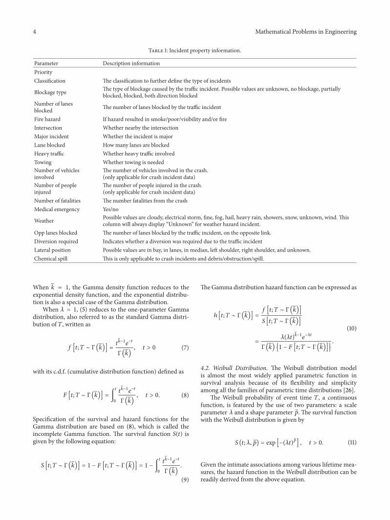
Table 1: Incident property information.

Parameter Description informationPriorityClassification The classification to further define the type of incidents

Blockage type The type of blockage caused by the traffic incident. Possible values are unknown, no blockage, partiallyblocked, blocked, both direction blocked

Number of lanesblocked The number of lanes blocked by the traffic incident

Fire hazard If hazard resulted in smoke/poor/visibility and/or fireIntersection Whether nearby the intersectionMajor incident Whether the incident is majorLane blocked How many lanes are blockedHeavy traffic Whether heavy traffic involvedTowing Whether towing is neededNumber of vehiclesinvolved

The number of vehicles involved in the crash.(only applicable for crash incident data)

Number of peopleinjured

The number of people injured in the crash.(only applicable for crash incident data)

Number of fatalities The number fatalities from the crashMedical emergency Yes/no

Weather Possible values are cloudy, electrical storm, fine, fog, hail, heavy rain, showers, snow, unknown, wind. Thiscolumn will always display “Unknown” for weather hazard incident.

Opp lanes blocked The number of lanes blocked by the traffic incident, on the opposite link.Diversion required Indicates whether a diversion was required due to the traffic incidentLateral position Possible values are in bay, in lanes, in median, left shoulder, right shoulder, and unknown.Chemical spill This is only applicable to crash incidents and debris/obstruction/spill.

When �� = 1, the Gamma density function reduces to theexponential density function, and the exponential distribu-tion is also a special case of the Gamma distribution.

When 𝜆 = 1, (5) reduces to the one-parameter Gammadistribution, also referred to as the standard Gamma distri-bution of 𝑇, written as

𝑓 [𝑡; 𝑇 ∼ Γ (��)] =𝑡��−1𝑒−𝑡

Γ (��), 𝑡 > 0 (7)

with its c.d.f. (cumulative distribution function) defined as

𝐹 [𝑡; 𝑇 ∼ Γ (��)] = ∫𝑡

0

𝑡��−1𝑒−𝑡

Γ (��), 𝑡 > 0. (8)

Specification of the survival and hazard functions for theGamma distribution are based on (8), which is called theincomplete Gamma function. The survival function 𝑆(𝑡) isgiven by the following equation:

𝑆 [𝑡; 𝑇 ∼ Γ (��)] = 1 − 𝐹 [𝑡; 𝑇 ∼ Γ (��)] = 1 − ∫𝑡

0

𝑡��−1𝑒−𝑡

Γ (��).

(9)

TheGamma distribution hazard function can be expressed as

ℎ [𝑡; 𝑇 ∼ Γ (��)] =𝑓 [𝑡; 𝑇 ∼ Γ (��)]

𝑆 [𝑡; 𝑇 ∼ Γ (��)]

=𝜆(𝜆𝑡)��−1

𝑒−𝜆𝑡

Γ (��) {1 − 𝐹 [𝑡; 𝑇 ∼ Γ (��)]}.

(10)

4.2. Weibull Distribution. The Weibull distribution modelis almost the most widely applied parametric function insurvival analysis because of its flexibility and simplicityamong all the families of parametric time distributions [26].

The Weibull probability of event time 𝑇, a continuousfunction, is featured by the use of two parameters: a scaleparameter 𝜆 and a shape parameter 𝑝. The survival functionwith the Weibull distribution is given by

𝑆 (𝑡; 𝜆, 𝑝) = exp [−(𝜆𝑡)𝑝] , 𝑡 > 0. (11)

Given the intimate associations among various lifetime mea-sures, the hazard function in the Weibull distribution can bereadily derived from the above equation.


Consider

ℎ (𝑡; 𝜆, 𝑝) = −(𝑑/𝑑𝑡) 𝑒

−(𝜆𝑡)𝑝

𝑒−(𝜆𝑡)𝑝

=𝜆𝑝𝑡𝑝−1 exp [−(𝜆𝑡)

𝑝]

exp [−(𝜆𝑡)𝑝]

= 𝜆𝑝(𝜆𝑡)𝑝−1

.

(12)

The cumulative hazard function 𝐻(𝑡) can be expressed interms of 𝑆(𝑡), given by

𝐻(𝑡) = − log 𝑆 (𝑡) = − log{exp [−∫𝑡

0

ℎ (𝑢) 𝑑𝑢]} . (13)

Therefore, the cumulative hazard function 𝐻(𝑡; 𝜆, 𝑝) can bewritten as

𝐻(𝑡; 𝜆, 𝑝) = − log 𝑆 (𝑡; 𝜆, 𝑝) = − log {exp [−(𝜆𝑡)𝑝]}

= (𝜆𝑡)𝑝.

(14)

Taking natural Log values on both sides of (14), (14) can bewritten as

log [− log 𝑆 (𝑡; 𝜆, 𝑝)] = log 𝜆 + 𝑝 log 𝑡. (15)

Specifications of 𝑆(𝑡) and ℎ(𝑡) lead to the followingequation for the Weibull p.d.f. function:

𝑓 (𝑡; 𝜆, 𝑝) = ℎ (𝑡) 𝑆 (𝑡) = 𝜆𝑝(𝜆𝑡)𝑝−1 exp [−(𝜆𝑡)

𝑝] . (16)

Likewise, the c.d.f. at time 𝑡 is derived by

𝐹 (𝑡; 𝜆, 𝑝) = 1 − 𝑆 (𝑡; 𝜆, 𝑝) = 1 − exp [−(𝜆𝑡)𝑝] . (17)

Given 𝜆∗ = 1/𝜆, the Weibull hazard function can bereexpressed as

ℎ (𝑡; 𝜆∗, 𝑝) =

𝑝

𝜆∗(

𝑡

𝜆∗)𝑝−1

. (18)

4.3. Log-Logistic Distribution. The lognormal distribution iswidely used to describe events whose rate increases initiallyand decreases consistently afterwards. The Log-logistic dis-tribution of 𝑇 is the antilogarithm of the familiar logisticdistribution. Let 𝑌 = log𝑇. The density function of 𝑌 isdefined as the familiar logistic distribution [26]:

𝑓 (𝑦) =��−1 exp [(𝑦 − 𝜇) /��]

{1 + exp [(𝑦 − 𝜇)/��]}2, 𝑦 ∈ (−∞,∞) , (19)

where 𝜇 and �� are parameters for the logistic function of 𝑌,described as 𝑌 ∼ Logist(𝜇, ��). Let 𝜆 = exp(𝜇) and 𝑝 = ��−1.The antilogarithm of (19) is the density function of 𝑇:

𝑓 (𝑡) =(𝑝/𝜆) (𝑡/𝜆)

𝑝−1

[1 + (𝑡/𝜆)𝑝]2

, 𝑡 > 0, (20)

where 𝜆 and𝑝 are parameters of the Log-logistic distribution,written as 𝑇 ∼ LLogist(𝜆, 𝑝). The c.d.f. of 𝑇 is then given as

𝐹 [𝑡; 𝑇 ∼ LLogist (𝜆, 𝑝)] =1

1 + (𝑡/𝜆)−𝑝

. (21)

Therefore, the survival and hazard rate functions of 𝑇 canthen be readily derived as follows:

𝑆 [𝑡; 𝑇 ∼ LLogist (𝜆, 𝑝)] = 1 − 𝐹 [𝑡; 𝑇 ∼ LLogist (𝜆, 𝑝)]

=1

1 + (𝑡/𝜆)𝑝

ℎ [𝑡; 𝑇 ∼ LLogist (𝜆, 𝑝)] =𝑓 [𝑡; 𝑇 ∼ LLogist (𝜆, 𝑝)]

𝑆 [𝑡; 𝑇 ∼ LLogis𝑡 (𝜆, 𝑝)]

=(𝑝/𝜆) (𝑡/𝜆)

𝑝−1

1 + (𝑡/𝜆)𝑝

.

(22)

5. Model Result

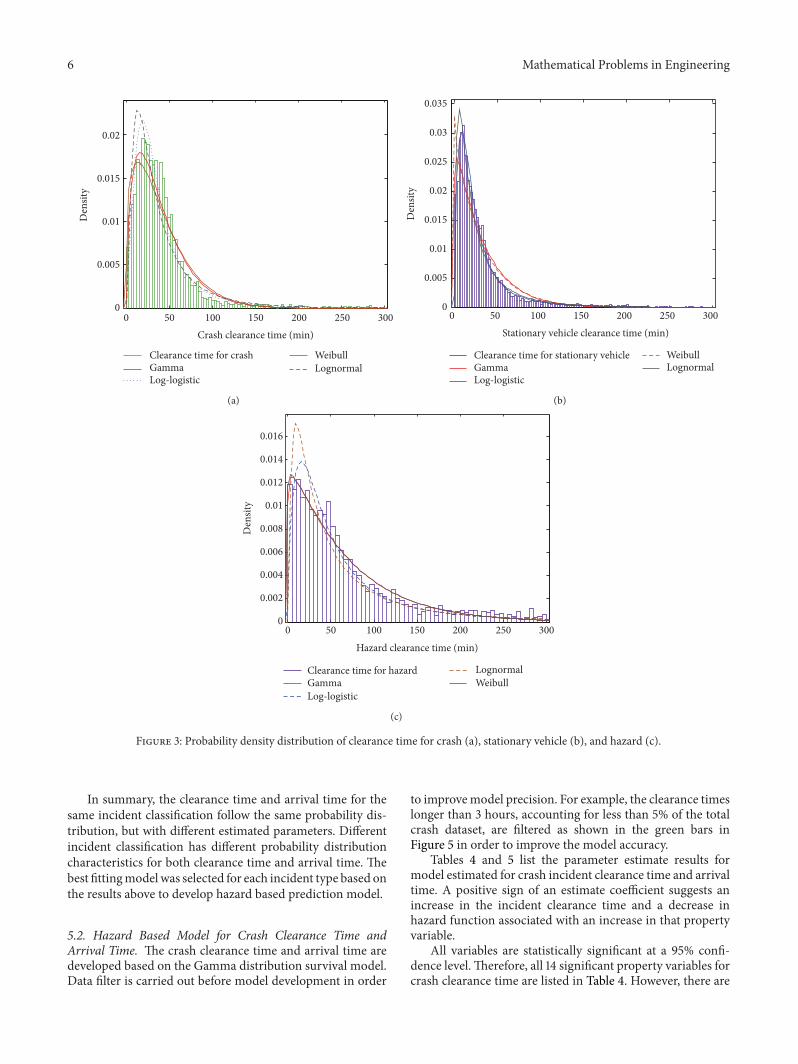
5.1. The Fitness of Distribution. Understanding of incidentcharacteristics and patterns is essential to establish an appro-priate prediction model; therefore, the statistical analysisis carried out firstly. There are 4966 crash records, 15791stationary vehicle data, and 3847 hazard records for clearancetime which are used to do distribution fitting analysis.Four probability density functions, which are Gamma, Log-logistic, Weibull, and lognormal, are fitted to the clearancetime for crash, stationary vehicle, and hazard incidents,respectively, (see Figures 3(a), 3(b), and 3(c)). Thick full linesindicate the best fitness distribution. The figures indicatethat each incident classification has its respective best fitnessdistribution function. Four parameters estimates of clearancetime probability density distribution: Log likelihood, domainmean, and variance are listed in Table 2. Log likelihood andvariance statistics indicate the goodness of fit distribution.

The less the variance is, the better the distribution fittingwill be. For example the Gamma distribution variance forcrash clearance time is 967.94, which is the least one com-paring other distributions. It is clearly shown that Gammadistribution is best fit for crash clearance time, Log-logisticfor stationary vehicle, and Weibull for the hazard.

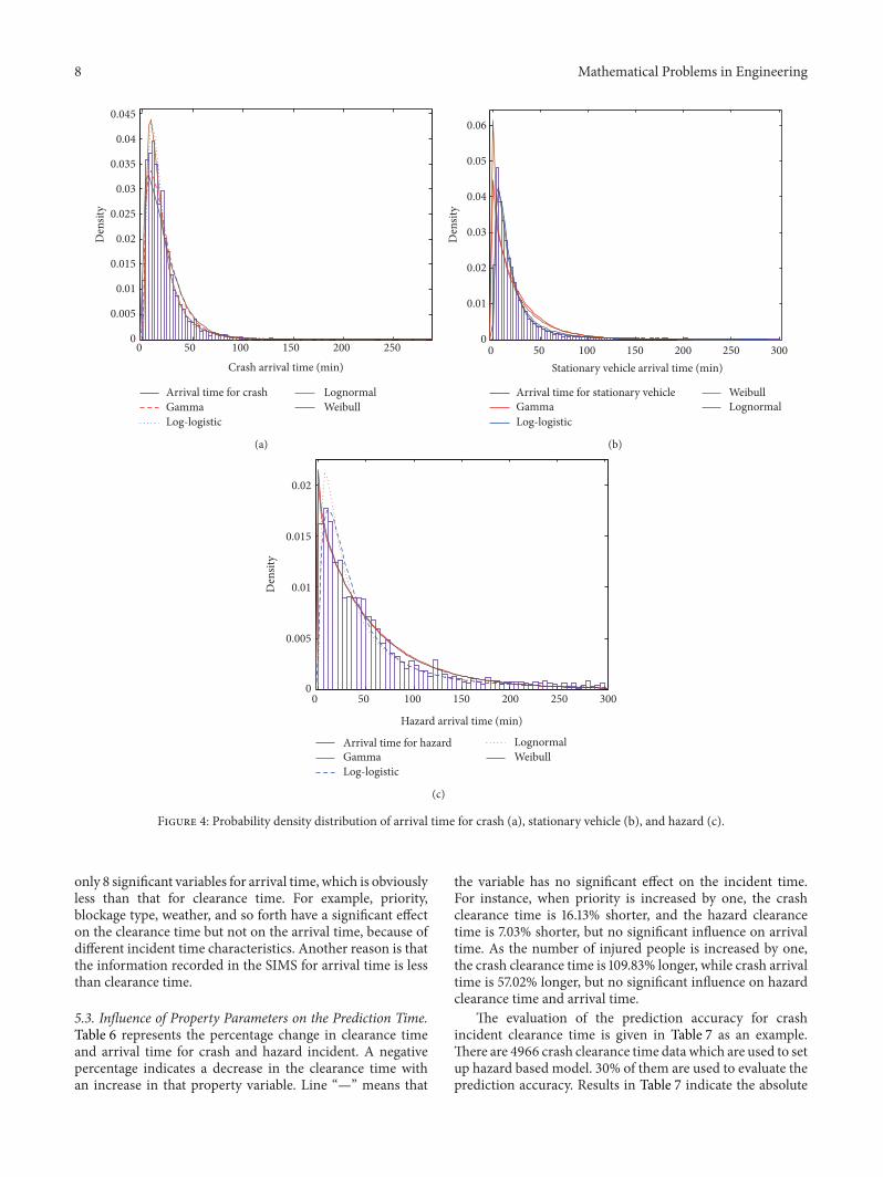
There are totally 4569 crashes, 14665 stationary vehicledata, and 3382 hazard records for arrival time which areused in this distribution fitting. The number of arrival timerecord is less than the counterpart for clearance time, becausethere exists an abundant of invalid arrival time data recordsin SIMS. All the invalid and defective data are filtered.Figures 4(a), 4(b), and 4(c) represent the probability densitydistributions of arrival time for crash, stationary vehicle, andhazard separately. Table 3 lists the parameters estimates ofarrival time probability density distribution for each incidenttype. Both the estimate parameters and the figure indicatethat the Gamma distribution is best fit for crash arrival time,Log-logistic for stationary vehicle, andWeibull for the hazard.


0 50 100 150 200 250 3000

0.005

0.01

0.015

0.02

Den

sity

Clearance time for crash

Crash clearance time (min)

GammaLog-logistic

WeibullLognormal

(a)

0 50 100 150 200 250 3000

0.005

0.01

0.015

0.02

0.025

0.03

0.035

Den

sity

Clearance time for stationary vehicle

Stationary vehicle clearance time (min)

GammaLog-logistic

WeibullLognormal

(b)

0 50 100 150 200 250 3000

0.002

0.004

0.006

0.008

0.01

0.012

0.014

0.016

Den

sity

Clearance time for hazard

Hazard clearance time (min)

GammaLog-logistic

LognormalWeibull

(c)

Figure 3: Probability density distribution of clearance time for crash (a), stationary vehicle (b), and hazard (c).

In summary, the clearance time and arrival time for thesame incident classification follow the same probability dis-tribution, but with different estimated parameters. Differentincident classification has different probability distributioncharacteristics for both clearance time and arrival time. Thebest fittingmodelwas selected for each incident type based onthe results above to develop hazard based prediction model.

5.2. Hazard Based Model for Crash Clearance Time andArrival Time. The crash clearance time and arrival time aredeveloped based on the Gamma distribution survival model.Data filter is carried out before model development in order

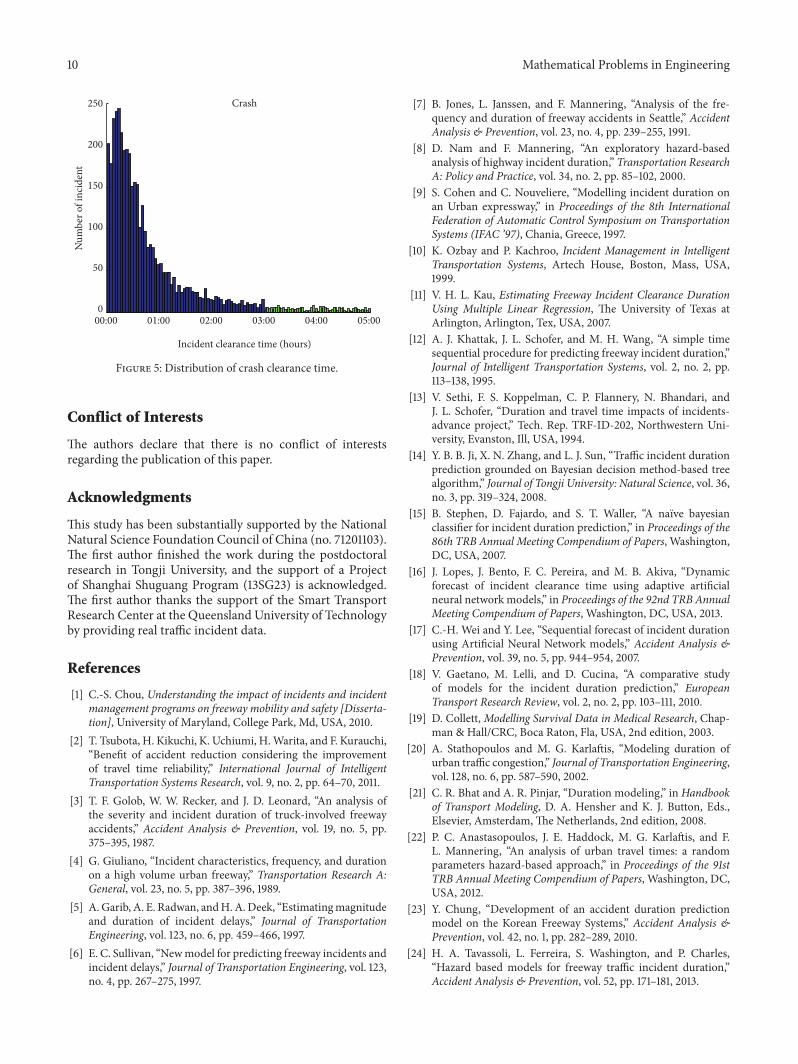
to improvemodel precision. For example, the clearance timeslonger than 3 hours, accounting for less than 5% of the totalcrash dataset, are filtered as shown in the green bars inFigure 5 in order to improve the model accuracy.

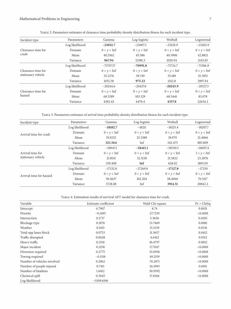
Tables 4 and 5 list the parameter estimate results formodel estimated for crash incident clearance time and arrivaltime. A positive sign of an estimate coefficient suggests anincrease in the incident clearance time and a decrease inhazard function associated with an increase in that propertyvariable.

All variables are statistically significant at a 95% confi-dence level.Therefore, all 14 significant property variables forcrash clearance time are listed in Table 4. However, there are


Table 2: Parameters estimates of clearance time probability density distribution fitness for each incident type.

Incident type Parameters Gamma Log-logistic Weibull Lognormal

Clearance time forcrash

Log likelihood −23032.7 −23007.3 −23128.9 −23202.9Domain 0 < y < Inf 0 < y < Inf 0 < y < Inf 0 < y < InfMean 40.3562 45.586 40.5906 42.8821

Variance 967.94 11380.3 1020.94 2143.83

Clearance time forstationary vehicle


Variance 1032.58 975.23 1142.8 2897.44

Clearance time forhazard


Variance 4382.43 4478.4 4357.8 22634.2

Table 3: Parameters estimates of arrival time probability density distribution fitness for each incident type.

Incident type Parameters Gamma Log-logistic Weibull Lognormal

Arrival time for crash

Log likelihood −18182.7 −18211 −18215.4 −18207.7Domain 0 < y < Inf 0 < y < Inf 0 < y < Inf 0 < y < InfMean 19.9232 25.3389 19.979 21.4866

Variance 323.564 Inf 343.475 885.809

Arrival time forstationary vehicle


Variance 559.408 Inf 628.02 1895.03

Arrival time for hazard

Log likelihood −17132.8 −17269.8 −17127.8 −17250Domain 0 < y < Inf 0 < y < Inf 0 < y < Inf 0 < y < InfMean 58.4637 102.204 58.4066 70.5117

Variance 3728.08 Inf 3914.51 20842.2

Table 4: Estimation results of survival AFT model for clearance time for crash.

Variable Estimate coefficient Wald Chi-square Pr > ChiSqIntercept 4.7907 8.74 0.0031Priority −0.1495 27.7239 <0.0001Intersection 0.1737 5.3656 0.0205Blockage type 0.1878 13.7469 0.0081Weather 0.1103 15.1529 0.0341Total opp lanes block 0.0753 11.5657 0.0412Traffic disrupted 0.0628 4.6412 0.0312Heavy traffic 0.1356 10.4797 0.0012Major incident 0.2158 17.7047 <0.0001Diversion required 0.2775 33.0936 <0.0001Towing required −0.1518 49.2159 <0.0001Number of vehicles involved 0.2862 70.2871 <0.0001Number of people injured 0.7411 26.1993 0.0101Number of fatalities 1.0412 30.9592 <0.0001Chemical spill 0.3045 17.4566 <0.0001Log likelihood −5509.6196


0 50 100 150 200 2500

0.005

0.01

0.015

0.02

0.025

0.03

0.035

0.04

0.045D

ensit

y

Arrival time for crash

Crash arrival time (min)

GammaLog-logistic

LognormalWeibull

(a)

0 50 100 150 200 250 3000

0.01

0.02

0.03

0.04

0.05

0.06

Den

sity

Arrival time for stationary vehicle

Stationary vehicle arrival time (min)

GammaLog-logistic

WeibullLognormal

(b)

0 50 100 150 200 250 3000

0.005

0.01

0.015

0.02

Den

sity

Arrival time for hazard

Hazard arrival time (min)

GammaLog-logistic

LognormalWeibull

(c)

Figure 4: Probability density distribution of arrival time for crash (a), stationary vehicle (b), and hazard (c).

only 8 significant variables for arrival time, which is obviouslyless than that for clearance time. For example, priority,blockage type, weather, and so forth have a significant effecton the clearance time but not on the arrival time, because ofdifferent incident time characteristics. Another reason is thatthe information recorded in the SIMS for arrival time is lessthan clearance time.

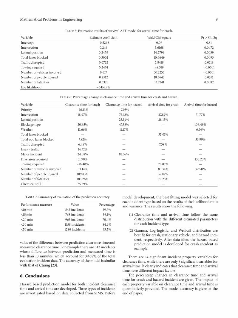
5.3. Influence of Property Parameters on the Prediction Time.Table 6 represents the percentage change in clearance timeand arrival time for crash and hazard incident. A negativepercentage indicates a decrease in the clearance time withan increase in that property variable. Line “—” means that

the variable has no significant effect on the incident time.For instance, when priority is increased by one, the crashclearance time is 16.13% shorter, and the hazard clearancetime is 7.03% shorter, but no significant influence on arrivaltime. As the number of injured people is increased by one,the crash clearance time is 109.83% longer, while crash arrivaltime is 57.02% longer, but no significant influence on hazardclearance time and arrival time.

The evaluation of the prediction accuracy for crashincident clearance time is given in Table 7 as an example.There are 4966 crash clearance time data which are used to setup hazard based model. 30% of them are used to evaluate theprediction accuracy. Results in Table 7 indicate the absolute


Table 5: Estimation results of survival AFT model for arrival time for crash.

Variable Estimate coefficient Wald Chi-square Pr > ChiSqIntercept −0.5248 0.06 0.81Intersection 0.246 3.6168 0.0472Lateral position 0.2479 14.2799 0.0039Total lanes blocked 0.3002 10.6649 0.0493Traffic disrupted 0.0732 2.8418 0.0218Towing required 0.2474 48.519 <0.0001Number of vehicles involved 0.617 57.2253 <0.0001Number of people injured 0.4512 18.3643 0.0351Number of fatalities 0.5321 13.7241 0.0082Log likelihood −6416.712

Table 6: Percentage change in clearance time and arrival time for crash and hazard.

Variable Clearance time for crash Clearance time for hazard Arrival time for crash Arrival time for hazardPriority −16.13% −7.03% — —Intersection 18.97% 73.13% 27.89% 71.77%Lateral position — 25.54% 28.13% —Blockage type 20.65% 47.38% — 106.49%Weather 11.66% 11.17% — 6.56%Total lanes blocked — — 35.01% —Total opp lanes blocked 7.82% — — 33.99%Traffic disrupted 6.48% — 7.59% —Heavy traffic 14.52% — — —Major incident 24.08% 81.56% — —Diversion required 31.98% — — 130.23%Towing required −16.40% — 28.07% —Number of vehicles involved 33.14% — 85.34% 377.41%Number of people injured 109.83% — 57.02% —Number of fatalities 183.26% — 70.25% —Chemical spill 35.59% — — —

Table 7: Summary of evaluation of the prediction accuracy.

Performance measure Value Percentage<10min 543 incidents 39.7%<15min 768 incidents 56.1%<20min 963 incidents 70.4%<30min 1158 incidents 84.6%<50min 1280 incidents 93.5%

value of the difference between prediction clearance time andmeasured clearance time. For example there are 543 incidentswhose difference between prediction and measured time isless than 10 minutes, which account for 39.68% of the totalevaluation incident data.The accuracy of themodel is similarwith that of Chung [23].

6. Conclusions

Hazard based prediction model for both incident clearancetime and arrival time are developed. Three types of incidentsare investigated based on data collected from SIMS. Before

model development, the best fitting model was selected foreach incident type based on the results of the likelihood ratioand variance. The results show the following.

(1) Clearance time and arrival time follow the samedistribution with the different estimated parametersfor each incident type.

(2) Gamma, Log-logistic, and Weibull distribution arebest fit for crash, stationary vehicle, and hazard inci-dent, respectively. After data filter, the hazard basedprediction model is developed for crash incident asexample.

There are 14 significant incident property variables forclearance time, while there are only 8 significant variables forarrival time. It clearly indicates that clearance time and arrivaltime have different impact factors.

The percentage changes in clearance time and arrivaltime for crash and hazard incident are given. The impact ofeach property variable on clearance time and arrival time isquantitatively provided. The model accuracy is given at theend of paper.


00:00 01:00 02:00 03:00 04:00 05:000

50

100

150

200

250

Incident clearance time (hours)

Num

ber o

f inc

iden

t

Crash

Figure 5: Distribution of crash clearance time.

Conflict of Interests

The authors declare that there is no conflict of interestsregarding the publication of this paper.

Acknowledgments

This study has been substantially supported by the NationalNatural Science Foundation Council of China (no. 71201103).The first author finished the work during the postdoctoralresearch in Tongji University, and the support of a Projectof Shanghai Shuguang Program (13SG23) is acknowledged.The first author thanks the support of the Smart TransportResearch Center at the Queensland University of Technologyby providing real traffic incident data.

References

[1] C.-S. Chou, Understanding the impact of incidents and incidentmanagement programs on freeway mobility and safety [Disserta-tion], University of Maryland, College Park, Md, USA, 2010.

[2] T. Tsubota, H. Kikuchi, K. Uchiumi, H.Warita, and F. Kurauchi,“Benefit of accident reduction considering the improvementof travel time reliability,” International Journal of IntelligentTransportation Systems Research, vol. 9, no. 2, pp. 64–70, 2011.

[3] T. F. Golob, W. W. Recker, and J. D. Leonard, “An analysis ofthe severity and incident duration of truck-involved freewayaccidents,” Accident Analysis & Prevention, vol. 19, no. 5, pp.375–395, 1987.

[4] G. Giuliano, “Incident characteristics, frequency, and durationon a high volume urban freeway,” Transportation Research A:General, vol. 23, no. 5, pp. 387–396, 1989.

[5] A.Garib, A. E. Radwan, andH.A.Deek, “Estimatingmagnitudeand duration of incident delays,” Journal of TransportationEngineering, vol. 123, no. 6, pp. 459–466, 1997.

[6] E. C. Sullivan, “Newmodel for predicting freeway incidents andincident delays,” Journal of Transportation Engineering, vol. 123,no. 4, pp. 267–275, 1997.

[7] B. Jones, L. Janssen, and F. Mannering, “Analysis of the fre-quency and duration of freeway accidents in Seattle,” AccidentAnalysis & Prevention, vol. 23, no. 4, pp. 239–255, 1991.

[8] D. Nam and F. Mannering, “An exploratory hazard-basedanalysis of highway incident duration,” Transportation ResearchA: Policy and Practice, vol. 34, no. 2, pp. 85–102, 2000.

[9] S. Cohen and C. Nouveliere, “Modelling incident duration onan Urban expressway,” in Proceedings of the 8th InternationalFederation of Automatic Control Symposium on TransportationSystems (IFAC ’97), Chania, Greece, 1997.

[10] K. Ozbay and P. Kachroo, Incident Management in IntelligentTransportation Systems, Artech House, Boston, Mass, USA,1999.

[11] V. H. L. Kau, Estimating Freeway Incident Clearance DurationUsing Multiple Linear Regression, The University of Texas atArlington, Arlington, Tex, USA, 2007.

[12] A. J. Khattak, J. L. Schofer, and M. H. Wang, “A simple timesequential procedure for predicting freeway incident duration,”Journal of Intelligent Transportation Systems, vol. 2, no. 2, pp.113–138, 1995.

[13] V. Sethi, F. S. Koppelman, C. P. Flannery, N. Bhandari, andJ. L. Schofer, “Duration and travel time impacts of incidents-advance project,” Tech. Rep. TRF-ID-202, Northwestern Uni-versity, Evanston, Ill, USA, 1994.

[14] Y. B. B. Ji, X. N. Zhang, and L. J. Sun, “Traffic incident durationprediction grounded on Bayesian decision method-based treealgorithm,” Journal of Tongji University: Natural Science, vol. 36,no. 3, pp. 319–324, 2008.

[15] B. Stephen, D. Fajardo, and S. T. Waller, “A naıve bayesianclassifier for incident duration prediction,” in Proceedings of the86th TRB Annual Meeting Compendium of Papers, Washington,DC, USA, 2007.

[16] J. Lopes, J. Bento, F. C. Pereira, and M. B. Akiva, “Dynamicforecast of incident clearance time using adaptive artificialneural network models,” in Proceedings of the 92nd TRB AnnualMeeting Compendium of Papers, Washington, DC, USA, 2013.

[17] C.-H. Wei and Y. Lee, “Sequential forecast of incident durationusing Artificial Neural Network models,” Accident Analysis &Prevention, vol. 39, no. 5, pp. 944–954, 2007.

[18] V. Gaetano, M. Lelli, and D. Cucina, “A comparative studyof models for the incident duration prediction,” EuropeanTransport Research Review, vol. 2, no. 2, pp. 103–111, 2010.

[19] D. Collett,Modelling Survival Data in Medical Research, Chap-man & Hall/CRC, Boca Raton, Fla, USA, 2nd edition, 2003.

[20] A. Stathopoulos and M. G. Karlaftis, “Modeling duration ofurban traffic congestion,” Journal of Transportation Engineering,vol. 128, no. 6, pp. 587–590, 2002.

[21] C. R. Bhat and A. R. Pinjar, “Duration modeling,” inHandbookof Transport Modeling, D. A. Hensher and K. J. Button, Eds.,Elsevier, Amsterdam, The Netherlands, 2nd edition, 2008.

[22] P. C. Anastasopoulos, J. E. Haddock, M. G. Karlaftis, and F.L. Mannering, “An analysis of urban travel times: a randomparameters hazard-based approach,” in Proceedings of the 91stTRB Annual Meeting Compendium of Papers, Washington, DC,USA, 2012.

[23] Y. Chung, “Development of an accident duration predictionmodel on the Korean Freeway Systems,” Accident Analysis &Prevention, vol. 42, no. 1, pp. 282–289, 2010.

[24] H. A. Tavassoli, L. Ferreira, S. Washington, and P. Charles,“Hazard based models for freeway traffic incident duration,”Accident Analysis & Prevention, vol. 52, pp. 171–181, 2013.


[25] D. A. Hensher and F. L. Mannering, “Hazard-based durationmodels and their application to transport analysis,” TransportReviews, vol. 14, no. 1, pp. 63–82, 1994.

[26] L. Xian, Survival Analysis: Models and Applications, HigherEducation Press, Beijing, China, 2012.

Submit your manuscripts athttp://www.hindawi.com

Hindawi Publishing Corporationhttp://www.hindawi.com Volume 2014

MathematicsJournal of


Mathematical Problems in Engineering

Hindawi Publishing Corporationhttp://www.hindawi.com

Differential EquationsInternational Journal of

Volume 2014

Applied MathematicsJournal of


Probability and StatisticsHindawi Publishing Corporationhttp://www.hindawi.com Volume 2014

Journal of


Mathematical PhysicsAdvances in

Complex AnalysisJournal of


OptimizationJournal of


CombinatoricsHindawi Publishing Corporationhttp://www.hindawi.com Volume 2014

International Journal of


Operations ResearchAdvances in

Journal of


Function Spaces

Abstract and Applied AnalysisHindawi Publishing Corporationhttp://www.hindawi.com Volume 2014

International Journal of Mathematics and Mathematical Sciences


The Scientific World JournalHindawi Publishing Corporation http://www.hindawi.com Volume 2014


Algebra

Discrete Dynamics in Nature and Society



Decision SciencesAdvances in

Discrete MathematicsJournal of

Hindawi Publishing Corporationhttp://www.hindawi.com

Volume 2014 Hindawi Publishing Corporationhttp://www.hindawi.com Volume 2014

Stochastic AnalysisInternational Journal of

Documents

Research Article Traffic Incident Clearance Time and