Embed Size (px)
Citation preview
Research ArticleShip Pipe Routing Design Using NSGA-II andCoevolutionary Algorithm
Wentie Niu, Haiteng Sui, Yaxiao Niu, Kunhai Cai, and Weiguo Gao
Key Laboratory of MechanismTheory and Equipment Design of Ministry of Education, Tianjin University, Tianjin 300072, China
Correspondence should be addressed to Wentie Niu; [email protected]
Received 9 July 2016; Revised 6 November 2016; Accepted 30 November 2016
Academic Editor: Francisco Chicano
Copyright © 2016 Wentie Niu et al. This is an open access article distributed under the Creative Commons Attribution License,which permits unrestricted use, distribution, and reproduction in any medium, provided the original work is properly cited.
Pipe route design plays a prominent role in ship design. Due to the complex configuration in layout space with numerous pipelines,diverse design constraints, and obstacles, it is a complicated and time-consuming process to obtain the optimal route of ship pipes.In this article, an optimized design method for branch pipe routing is proposed to improve design efficiency and to reduce humanerrors. By simplifying equipment and ship hull models and dividing workspace into three-dimensional grid cells, the mathematicmodel of layout space is constructed. Based on the proposed concept of pipe grading method, the optimization model of piperouting is established. Then an optimization procedure is presented to deal with pipe route planning problem by combining mazealgorithm (MA), nondominated sorting genetic algorithm II (NSGA-II), and cooperative coevolutionary nondominated sortinggenetic algorithm II (CCNSGA-II). To improve the performance in genetic algorithm procedure, a fixed-length encoding methodis presented based on improved maze algorithm and adaptive region strategy. Fuzzy set theory is employed to extract the bestcompromise pipeline from Pareto optimal solutions. Simulation test of branch pipe and design optimization of a fuel piping systemwere carried out to illustrate the design optimization procedure in detail and to verify the feasibility and effectiveness of the proposedmethodology.
1. Introduction
Since the 1970s, pipe routing design has been studied in var-ious industrial fields, like aeroengine, large-scale integratedcircuit, ship, and so forth. Pipe routing design, which isrelated to other tasks, is one of the most important processesat the detailed design stage of a ship. However, duo tothe complexity of piping system and the diversity of con-straints in ship piping system, it is time-consuming anddifficult to achieve feasible layout. Therefore, it is significantto investigate automatic pipe routing method.
Systematic studies in route path planning have beencarried out by researchers for several decades. Dijkstraalgorithm [1] proposed in 1959 is a well-known algorithmfor path optimization with shortest length. Based on Dijkstraalgorithm, 𝐴∗ algorithm is developed by Hart et al. [2]to improve search efficiency. In 1961, Lee [3] proposedmaze algorithm to solve connecting problem of two points.However, huge data storage is essential to handle large-sizeoptimization problems, which results in low search efficiency.
To overcome thementioned drawbacks, numerous researcheshave been conducted in references [4–8]. Typically, the escapealgorithm is proposed by Hightower [4] to improve searchefficiency, but an optimal solution also cannot be guaranteed.Recently, researches on piping route path planning havebeen promoted by the development of modern optimizationalgorithms such as genetic algorithm [9–17], ant colonyalgorithm [18–23], and particle swarm optimization [24–27].Genetic algorithm is used by Ito [10] to optimize pipe routingin two-dimensional space, in which the chromosome of routepath with variable-length is firstly defined. Afterward, thechromosome with fixed length [12] is redefined to solve theproblems such as low efficiency in GA. A variable-lengthencoding technique is proposed by Fan et al. [13] and appliedto optimize the ship pipe paths in three-dimensional space,which leads to the complexity of algorithm design process. Inaddition, expert systems [28–31] are also applied in ship piperoute design.
At present, the optimization algorithm research on piperoute planning mainly concentrates on the case with two
Hindawi Publishing CorporationMathematical Problems in EngineeringVolume 2016, Article ID 7912863, 21 pageshttp://dx.doi.org/10.1155/2016/7912863
2 Mathematical Problems in Engineering
terminals, while multibranch pipe design is rarely studied.Park and Storch [29] developed a cell-generation method forpipe routing in a ship engine room, in which the branchpipeline is regarded as a compound of two simple forms: end-forked andmiddle-forked. Usingmaze algorithm and Steinertree theory, Fan et al. [7] conduct the research on pipe routingproblem of aeroengine. Coevolutionary algorithm is appliedbyWu et al. [32] for multibranch pipe routing in ship. Steinerminimal tree and particle swarm optimization are combinedby Liu and Wang [33] to solve the optimization problemof multibranch pipe routing in aeroengine. However, fewerresearchers have taken the differences of pipeline diametersinto consideration. When pulsating pressure is existing inpipeline, the excitation force will be generated at the branchpoint because of the big difference in diameter value of theconnected pipes, which further influences working periodand usage security of pipeline [34]. Therefore, the diameterdifferences should be taken into consideration in optimiza-tion algorithm.
Owing to the diameter differences of branch pipelines,the concept of pipe grading is defined in this paper. Inconsideration of the number differences of connecting pointsin each grade, a new algorithm is proposed by combiningmaze algorithm (MA) [3], nondominated sorting geneticalgorithm II (NSGA-II) [35], and cooperative coevolutionarynondominated sorting genetic algorithm II (CCNSGA-II)[36]. To improve the performance in genetic algorithmprocedure, a fixed-length encoding method is presentedbased on the improved maze algorithm and adaptive regionstrategy. In addition, fuzzy set theory is employed to extractthe best compromise pipeline from Pareto optimal solutions,by which the imprecise nature of decision maker’s judgmentis avoided.
The rest of this paper is organized as follows.The problemof ship pipe route design is formulated in Section 2. Theproposed pipe routing algorithm is presented in Section 3. Acase study is conducted to verify the proposed algorithm inSection 4. Finally, conclusions are drawn in Section 5.
2. Problem Formulation
2.1. Representation of Piping Layout Space. Due to the com-plex ship hull structure and diverse equipment with variousshapes, it is time-consuming and inefficient to describe allgeometric information in detail for pipe routing design inship piping layout space. Therefore, it is essential to simplifythe environment of ship piping layout. To construct a reason-able workspace model representing the essential geometricinformation of the equipment and ship hull structure, severalprinciples should be obeyed in the environment simplifica-tion of piping layout.
(1) The geometrical properties of the model should besimple;
(2) Spatial position of the model should be expressedaccurately;
(3) The accurate spatial positions of the pipeline termi-nals should be guaranteed.
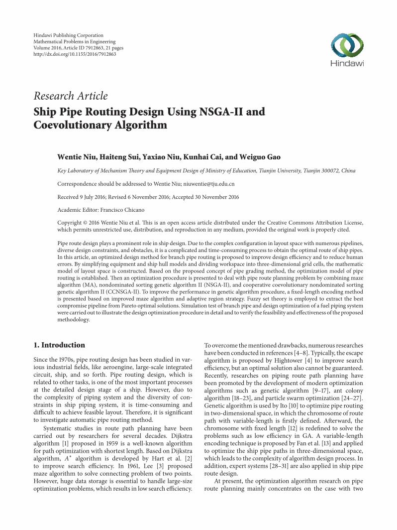
2.1.1. Simplification of Equipment Model. Informationallycomplete models are proposed in literature [37] for designconstraints based on an analysis of geometric and nonge-ometric properties of the related space volumes, which issuitable for component layout problem. For the problem ofpiping system layout, since the equipment locations havealready been determined, the simplification of componentsis just required, and the simplest approach is to establish axisaligned bounding box (AABB). However, if the equipmentmodel is complex, it is difficult for AABB to meet therequirements for accurate expression of spatial location. Asshown in Figure 1, the equipment model simplified by AABBis illustrated in Figure 1(b), inwhich themodel information oforiginal equipment in Figure 1(a) is not described accurately.In this paper, the optimized subdivision boundary boxmethod described in literature [38] is introduced to simplifythe models of ship equipment, an example of simplificationis shown in Figure 1(c), and other equipment involved inlayout space are simplified by the same way. The proce-dures of optimized subdivision boundary box method are asfollows.
Step 1. Construct the AABB of the equipment model.
Step 2. Divide AABB by using the nonuniform grid of cellsaccording to the characteristics of the equipment.
Step 3. For each cell, find the polygons of the model that lieinside or intersect with it.
Step 4. Construct the AABB of the polygons by Step 3.
Step 5. Clip the AABB with the cell itself.
Step 6. Loop to Step 3 until all cells in the grid are processed.
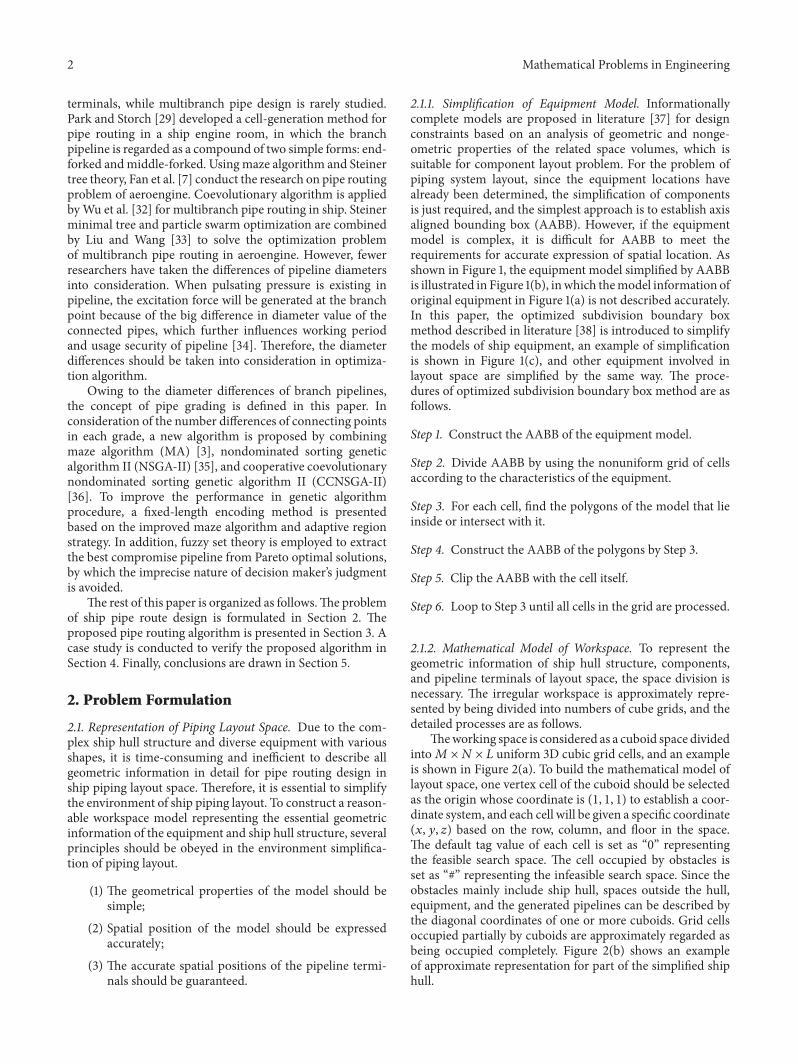
2.1.2. Mathematical Model of Workspace. To represent thegeometric information of ship hull structure, components,and pipeline terminals of layout space, the space division isnecessary. The irregular workspace is approximately repre-sented by being divided into numbers of cube grids, and thedetailed processes are as follows.
Theworking space is considered as a cuboid space dividedinto𝑀×𝑁 × 𝐿 uniform 3D cubic grid cells, and an exampleis shown in Figure 2(a). To build the mathematical model oflayout space, one vertex cell of the cuboid should be selectedas the origin whose coordinate is (1, 1, 1) to establish a coor-dinate system, and each cell will be given a specific coordinate(𝑥, 𝑦, 𝑧) based on the row, column, and floor in the space.The default tag value of each cell is set as “0” representingthe feasible search space. The cell occupied by obstacles isset as “#” representing the infeasible search space. Since theobstacles mainly include ship hull, spaces outside the hull,equipment, and the generated pipelines can be described bythe diagonal coordinates of one or more cuboids. Grid cellsoccupied partially by cuboids are approximately regarded asbeing occupied completely. Figure 2(b) shows an exampleof approximate representation for part of the simplified shiphull.
Mathematical Problems in Engineering 3
(a)
(b)
(c)
Figure 1: An example for simplification of the equipment model.
x
y
z
Ship hull
Cells on obstacle
(a) (b)
Figure 2: Mathematical model of workspace. (a) Grid method. (b) An example of approximate representation for the simplified ship hull.
2.2. Description of Pipe Information
2.2.1. Redefinition of Connecting Point. Since the inlet/outletof equipment is involved in the simplified model, the equip-ment simplification will result in failed connection of thepipeline terminals in model space. To solve this problem, theactual inlet/outlet involved in one or several grids is extendedto the adjacent grids outside the simplified model along itsnormal. And the adjacent grid cell passed by the axis ofinlet/outlet is defined as new connecting point.
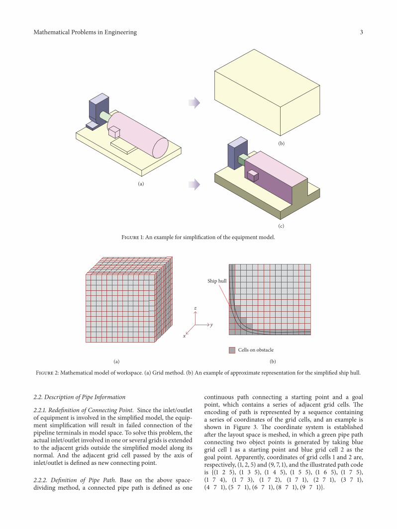
2.2.2. Definition of Pipe Path. Base on the above space-dividing method, a connected pipe path is defined as one
continuous path connecting a starting point and a goalpoint, which contains a series of adjacent grid cells. Theencoding of path is represented by a sequence containinga series of coordinates of the grid cells, and an example isshown in Figure 3. The coordinate system is establishedafter the layout space is meshed, in which a green pipe pathconnecting two object points is generated by taking bluegrid cell 1 as a starting point and blue grid cell 2 as thegoal point. Apparently, coordinates of grid cells 1 and 2 are,respectively, (1, 2, 5) and (9, 7, 1), and the illustrated path codeis {(1 2 5), (1 3 5), (1 4 5), (1 5 5), (1 6 5), (1 7 5),(1 7 4), (1 7 3), (1 7 2), (1 7 1), (2 7 1), (3 7 1),(4 7 1), (5 7 1), (6 7 1), (8 7 1), (9 7 1)}.
4 Mathematical Problems in Engineering
1
2
Object point
Route path
x
y
z
Figure 3: Definition of pipe path.
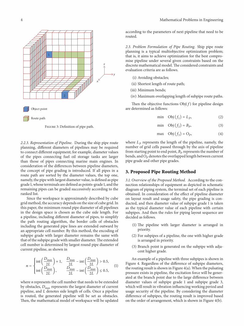
2.2.3. Representation of Pipeline. During the ship pipe routeplanning, different diameters of pipelines may be requiredto connect different equipment; for example, diameter valuesof the pipes connecting fuel oil storage tanks are largerthan those of pipes connecting marine main engines. Inconsideration of the differences between pipeline diameters,the concept of pipe grading is introduced. If all pipes in aroute path are sorted by the diameter values, the top one,namely, the pipewith largest diameter value, is defined as pipegrade 1, whose terminals are defined as points-grade 1, and theremaining pipes can be graded successively according to theranked list.
Since the workspace is approximately described by cubegridmethod, the accuracy depends on the size of cube grid. Inthis paper, the minimum round pipe diameter of all pipelinesin the design space is chosen as the cube side length. Fora pipeline, including different diameter of pipes, to simplifythe path routing algorithm, the border cells of obstaclesincluding the generated pipe lines are extended outward byan appropriate cell number. By this method, the encoding ofsubpipe grade with larger diameter remains the same withthat of the subpipe gradewith smaller diameter.The extendedcell number is determined by largest round pipe diameter ofcurrent pipeline, as shown in
𝑛 = {{{{{int(𝐷max2𝐿 ) + 1, 𝐷max2𝐿 − int(𝐷max2𝐿 ) > 0.5,int(𝐷max2𝐿 ) , 𝐷max2𝐿 − int(𝐷max2𝐿 ) ≤ 0.5, (1)
where 𝑛 represents the cell number that needs to be extendedby obstacles, 𝐷max represents the largest diameter of currentpipeline, and 𝐿 denotes side length of cells. Once a pipelineis routed, the generated pipeline will be set as obstacles.Then, the mathematical model of workspace will be updated
according to the parameters of next pipeline that need to berouted.
2.3. Problem Formulation of Pipe Routing. Ship pipe routeplanning is a typical multiobjective optimization problem;that is, it aims to achieve optimization for the best compro-mise pipeline under several given constraints based on thediscretemathematicalmodel.The considered constraints andevaluation criteria are as follows.
(i) Avoiding obstacles;(ii) Shortest length of route path;(iii) Minimum bends;(iv) Maximum overlapping length of subpipe route paths.
Then the objective functions Obj(𝑓) for pipeline designare determined as follows:
min Obj (𝑓1) = 𝐿𝑃, (2)
min Obj (𝑓2) = 𝐵𝑃, (3)
max Obj (𝑓3) = 𝑂𝑃, (4)
where 𝐿𝑃 represents the length of the pipeline, namely, thenumber of grid cells passed through by the axis of pipelinefrom starting point to end point, 𝐵𝑃 represents the number ofbends, and𝑂𝑃 denotes the overlapped length between currentpipe grade and other pipe grades.
3. Proposed Pipe Routing Method
3.1. Overview of the Proposed Method. According to the con-nection relationships of equipment as depicted in schematicdiagram of piping system, the terminal set of each pipeline isobtained. In consideration of the effect of pipeline diameteron layout result and usage safety, the pipe grading is con-ducted, and then diameter value of subpipe grade 1 is takenas the typical diameter value of each pipeline with certainsubpipes. And then the rules for piping layout sequence aredecided as follows.
(1) The pipeline with larger diameter is arranged inpriority.
(2) For subpipes of a pipeline, the one with higher gradeis arranged in priority.
(3) Branch point is generated on the subpipe with adja-cent higher grade.
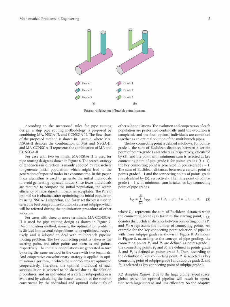
An example of a pipeline with three subpipes is shown inFigure 4. Regardless of the difference of subpipe diameters,the routing result is shown in Figure 4(a).When the pulsatingpressure exists in pipeline, the excitation force will be gener-ated at the branch point due to the large difference betweendiameter values of subpipe grade 1 and subpipe grade 3,which will result in vibration influencing working period andusage security of the pipeline. By considering the diameterdifference of subpipes, the routing result is improved basedon the order of arrangement, which is shown in Figure 4(b).
Mathematical Problems in Engineering 5
Grade 3
Grade 2
Grade 1
(a)
Grade 3
Grade 2
Grade 1
(b)
Figure 4: Selection of branch point location.
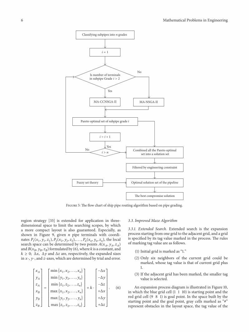
According to the mentioned rules for pipe routingdesign, a ship pipe routing methodology is proposed bycombining MA, NSGA-II, and CCNSGA-II. The flow chartof the proposed method is shown in Figure 5, where MA-NSGA-II denotes the combination of MA and NSGA-II,andMA-CCNSGA-II represents the combination of MA andCCNSGA-II.
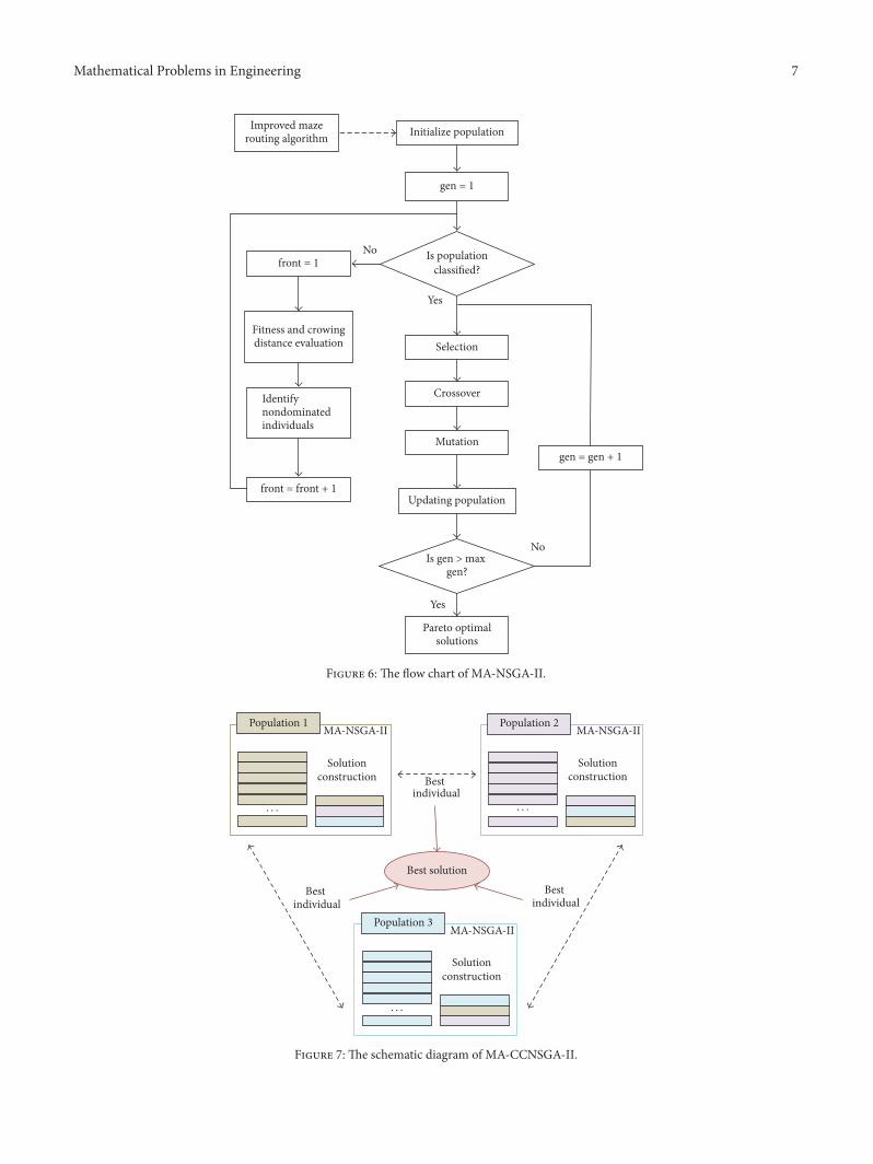
For case with two terminals, MA-NSGA-II is used forpipe routing design as shown in Figure 6.The search strategyof tendencies in direction is mainly adopted by researchersto generate initial population, which might lead to thegeneration of repeated nodes in a chromosome. In this paper,maze algorithm is used to generate the initial individualsto avoid generating repeated nodes. Since fewer individualsare required to compose the initial population, the searchefficiency of maze algorithm becomes acceptable. The Paretooptimal set is obtained after optimizing the initial populationby using NSGA-II algorithm, and fuzzy set theory is used toselect the best compromise solution of current subpipe, whichwill be referred during the optimization procedure of othersubpipes.
For cases with three or more terminals, MA-CCNSGA-II is used for pipe routing design as shown in Figure 7.Decomposition method, namely, the optimization problem,is divided into several subproblems to be optimized, respec-tively, and is adopted to deal with multibranch pipelinerouting problem. The key connecting point is taken as thestarting point, and other points are taken as end points,respectively. The initial subpopulations are generated in turnby using the same method in the cases with two terminals.And cooperative coevolutionary strategy is applied in opti-mization algorithm, in which the subproblems are optimizedcooperatively. Therefore, the optimal individual of eachsubpopulation is selected to be shared during the solutionprocedures, and an individual of a certain subpopulation isevaluated by calculating the fitness function of the solutionconstructed by the individual and optimal individuals of
other subpopulations.The evolution and cooperation of eachpopulation are performed continually until the evolution iscompleted, and the final optimal individuals are combinedtogether as an optimal solution of the multibranch pipes.
Thekey connecting point is defined as follows. For points-grade 1, the sum of Euclidean distances between a certainpoint of points-grade 1 and others is, respectively, calculatedby (5), and the point with minimum sum is selected as keyconnecting point of pipe grade 1; for points-grade 𝑖 (𝑖 > 1),the key connecting point is generated in points-grade 𝑖 − 1.The sum of Euclidean distances between a certain point ofpoints-grade 𝑖 − 1 and the connecting points of points-grade𝑖 is calculated by (5), respectively. Then, the point of points-grade 𝑖 − 1 with minimum sum is taken as key connectingpoint of pipe grade 𝑖.
𝐿𝑃𝑖 =𝑛∑𝑗=1
𝐿𝑃𝑖𝑃𝑗 , 𝑖 = 1, 2, . . . , 𝑛; 𝑗 = 1, 2, . . . , 𝑛, (5)
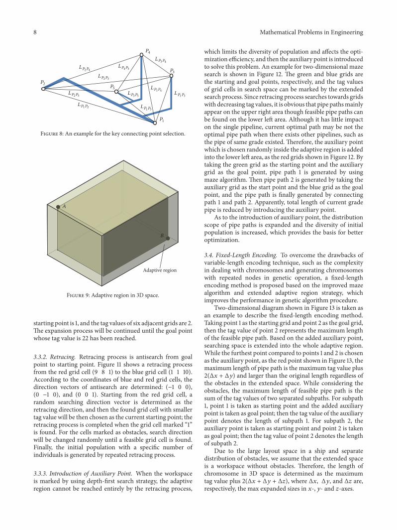
where 𝐿𝑃𝑖 represents the sum of Euclidean distances whenthe connecting point 𝑃𝑖 is taken as the starting point; 𝐿𝑃𝑖𝑃𝑗denotes the Euclidean distance between connecting points𝑃𝑖;and 𝑃𝑗; 𝑛 represents the number of connecting points. Anexample for the key connecting point selection of pipelinewith three subpipe grades is shown in Figure 8. As shownin Figure 8, according to the concept of pipe grading, theconnecting points 𝑃1 and 𝑃2 are defined as points-grade 1,the connecting points 𝑃3 and 𝑃4 are defined as points-grade2, and 𝑃5 is defined as points-grade 3. Then, according tothe definition of key connecting point, 𝑃1 is selected as keyconnecting point of subpipe grade 1 and subpipe grade 2, and𝑃4 is selected as key connecting point of subpipe grade 3.
3.2. Adaptive Region. Due to the huge piping layout space,global search for optimal pipeline will result in opera-tion with large storage and low efficiency. So the adaptive
6 Mathematical Problems in Engineering
MA-CCNSGA-II MA-NSGA-II
Pareto optimal set of subpipe grade i
Optimal solution set of the pipeline
YesNo
No
Yes
Fuzzy set theory
The best compromise solution
Filtered by engineering constraint
i = 1
i = i + 1
i > n
Is number of terminalsin subpipe Grade i > 2
Combined all the Pareto optimalset into a solution set
Classifying subpipes into n grades
Figure 5: The flow chart of ship pipe routing algorithm based on pipe grading.
region strategy [33] is extended for application in three-dimensional space to limit the searching scopes, by whicha more compact layout is also guaranteed. Especially, asshown in Figure 9, given 𝑛 pipe terminals with coordi-nates 𝑃1(𝑥1, 𝑦1, 𝑧1), 𝑃2(𝑥2, 𝑦2, 𝑧2), . . . , 𝑃𝑛(𝑥𝑛, 𝑦𝑛, 𝑧𝑛), the localsearch space can be determined by two points 𝐴(𝑥𝐴, 𝑦𝐴, 𝑧𝐴)and𝐵(𝑥𝐵, 𝑦𝐵, 𝑧𝐵) formulated by (6), where 𝑘 is a constant, and𝑘 ≥ 0; Δ𝑥, Δ𝑦 and Δ𝑧 are, respectively, the expanded sizesin 𝑥-, 𝑦-, and 𝑧-axes, which are determined by trial and error.
[[[[[[[[[[[[
𝑥𝐴𝑦𝐴𝑧𝐴𝑥𝐵𝑦𝐵𝑧𝐵
]]]]]]]]]]]]
=
[[[[[[[[[[[[
min {𝑥1, 𝑥2, . . . , 𝑥𝑛}min {𝑦1, 𝑦2, . . . , 𝑦𝑛}min {𝑧1, 𝑧2, . . . , 𝑧𝑛}max {𝑥1, 𝑥2, . . . , 𝑥𝑛}max {𝑦1, 𝑦2, . . . , 𝑦𝑛}max {𝑧1, 𝑧2, . . . , 𝑧𝑛}
]]]]]]]]]]]]
+ 𝑘 ⋅
[[[[[[[[[[[[
−Δ𝑥−Δ𝑦−Δ𝑧+Δ𝑥+Δ𝑦+Δ𝑧
]]]]]]]]]]]]
. (6)
3.3. Improved Maze Algorithm
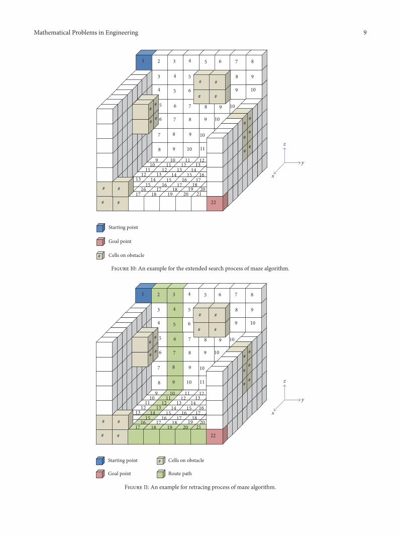
3.3.1. Extended Search. Extended search is the expansionprocess starting from one grid to the adjacent grid, and a gridis specified by its tag value marked in the process. The rulesof marking tag value are as follows.
(1) Initial grid is marked as “1.”(2) Only six neighbors of the current grid could be
marked, whose tag value is that of current grid plus1.
(3) If the adjacent grid has been marked, the smaller tagvalue is selected.
An expansion process diagram is illustrated in Figure 10,in which the blue grid cell (1 1 10) is starting point and thered grid cell (9 8 1) is goal point. In the space built by thestarting point and the goal point, gray cells marked as “#”represent obstacles in the layout space, the tag value of the
Mathematical Problems in Engineering 7
Initialize population
gen = 1
Is populationclassified?front = 1
Identifynondominatedindividuals
front = front + 1
Fitness and crowingdistance evaluation Selection
Crossover
Mutation
Updating population
Pareto optimalsolutions
gen = gen + 1
Is gen > max gen?
Improved mazerouting algorithm
Yes
No
Yes
No
Figure 6: The flow chart of MA-NSGA-II.
Bestindividual
Solutionconstruction
Population 2 MA-NSGA-II
Bestindividual
Bestindividual
Best solution
Solutionconstruction
Population 1MA-NSGA-II
Solutionconstruction
Population 3MA-NSGA-II
· · · · · ·
· · ·
Figure 7: The schematic diagram of MA-CCNSGA-II.
8 Mathematical Problems in Engineering
P2
LP2P4
LP2P5
LP2P3
LP1P2
LP4P5
P5
LP3P5
LP1P5
P4
LP1P4
P1
P3
LP3P4
LP1P3
Figure 8: An example for the key connecting point selection.
A
B
Adaptive region
Figure 9: Adaptive region in 3D space.
starting point is 1, and the tag values of six adjacent grids are 2.The expansion process will be continued until the goal pointwhose tag value is 22 has been reached.
3.3.2. Retracing. Retracing process is antisearch from goalpoint to starting point. Figure 11 shows a retracing processfrom the red grid cell (9 8 1) to the blue grid cell (1 1 10).According to the coordinates of blue and red grid cells, thedirection vectors of antisearch are determined: (−1 0 0),(0 −1 0), and (0 0 1). Starting from the red grid cell, arandom searching direction vector is determined as theretracing direction, and then the found grid cell with smallertag value will be then chosen as the current starting point; theretracing process is completed when the grid cell marked “1”is found. For the cells marked as obstacles, search directionwill be changed randomly until a feasible grid cell is found.Finally, the initial population with a specific number ofindividuals is generated by repeated retracing process.
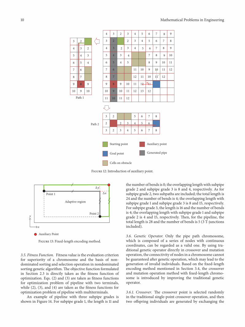
3.3.3. Introduction of Auxiliary Point. When the workspaceis marked by using depth-first search strategy, the adaptiveregion cannot be reached entirely by the retracing process,
which limits the diversity of population and affects the opti-mization efficiency, and then the auxiliary point is introducedto solve this problem. An example for two-dimensional mazesearch is shown in Figure 12. The green and blue grids arethe starting and goal points, respectively, and the tag valuesof grid cells in search space can be marked by the extendedsearch process. Since retracing process searches towards gridswith decreasing tag values, it is obvious that pipe pathsmainlyappear on the upper right area though feasible pipe paths canbe found on the lower left area. Although it has little impacton the single pipeline, current optimal path may be not theoptimal pipe path when there exists other pipelines, such asthe pipe of same grade existed. Therefore, the auxiliary pointwhich is chosen randomly inside the adaptive region is addedinto the lower left area, as the red grids shown in Figure 12. Bytaking the green grid as the starting point and the auxiliarygrid as the goal point, pipe path 1 is generated by usingmaze algorithm. Then pipe path 2 is generated by taking theauxiliary grid as the start point and the blue grid as the goalpoint, and the pipe path is finally generated by connectingpath 1 and path 2. Apparently, total length of current gradepipe is reduced by introducing the auxiliary point.
As to the introduction of auxiliary point, the distributionscope of pipe paths is expanded and the diversity of initialpopulation is increased, which provides the basis for betteroptimization.
3.4. Fixed-Length Encoding. To overcome the drawbacks ofvariable-length encoding technique, such as the complexityin dealing with chromosomes and generating chromosomeswith repeated nodes in genetic operation, a fixed-lengthencoding method is proposed based on the improved mazealgorithm and extended adaptive region strategy, whichimproves the performance in genetic algorithm procedure.
Two-dimensional diagram shown in Figure 13 is taken asan example to describe the fixed-length encoding method.Taking point 1 as the starting grid and point 2 as the goal grid,then the tag value of point 2 represents the maximum lengthof the feasible pipe path. Based on the added auxiliary point,searching space is extended into the whole adaptive region.While the furthest point compared to points 1 and 2 is chosenas the auxiliary point, as the red point shown in Figure 13, themaximum length of pipe path is the maximum tag value plus2(Δ𝑥 + Δ𝑦) and larger than the original length regardless ofthe obstacles in the extended space. While considering theobstacles, the maximum length of feasible pipe path is thesum of the tag values of two separated subpaths. For subpath1, point 1 is taken as starting point and the added auxiliarypoint is taken as goal point; then the tag value of the auxiliarypoint denotes the length of subpath 1. For subpath 2, theauxiliary point is taken as starting point and point 2 is takenas goal point; then the tag value of point 2 denotes the lengthof subpath 2.
Due to the large layout space in a ship and separatedistribution of obstacles, we assume that the extended spaceis a workspace without obstacles. Therefore, the length ofchromosome in 3D space is determined as the maximumtag value plus 2(Δ𝑥 + Δ𝑦 + Δ𝑧), where Δ𝑥, Δ𝑦, and Δ𝑧 are,respectively, the max expanded sizes in 𝑥-, 𝑦- and 𝑧-axes.
Mathematical Problems in Engineering 9
Starting point
Goal point
# Cells on obstacle
5#
1 2
5
4
3
3
4 5
54 6
6
6 7
7
7
7
6
8
8
8
8
8
9
109
9
9
9 10
10
10
#
##
#
9
8 9 10 11
#
# #
1010
1111
11
1212
1212
1313
1313 14
1414
15
1515 16
16
1616
1717
1717
1818
1819
19 2020
2122
#
#
##
#
##
##
#
z
x
y
Figure 10: An example for the extended search process of maze algorithm.
Starting point
Goal point
# Cells on obstacle
Route path
5#
1 2
5
4
3
3
4 5
54 6
6
6 7
7
7
7
6
8
8
8
8
8
9
109
9
9
9 10
10
10
#
##
#
9
8 9 10 11
#
# #
1010
1111
11
1212
1212
1313
1313 14
1414
15
1515 16
16
1616
1717
1717
1818
1819
19 2020
2122
#
#
##
#
##
##
#
z
x
y
Figure 11: An example for retracing process of maze algorithm.
10 Mathematical Problems in Engineering
3 2
4 3 2
5 4 3
6 5 4
7 6
8 7
9 8 9
Path 1
Path 2
4 3 2 3 4 5 6 7 8 9
3 2 3 4 5 6 7 8
4 3 2 3 4 5 6 7 8 9
5 4 3 4 7 8 9 10
6 5 4 5 8 9 10 11
7 6 11 10 9 10 11 12
8 7 12 11 10 11 12
9 8 9 10 11 12 11
10 9 10 11 12 13 12
11 10 11 12
2
3 2 5 6 7 8
2 3 4 5 6
3 2 3 4 5 6 7 8
2
Starting point
Goal point
Cells on obstacle
Auxiliary point
Generated pipe
10910
Figure 12: Introduction of auxiliary point.
Adaptive region
Point 1
Point 2
x
y
Auxiliary Point
Δx
Δy
Figure 13: Fixed-length encoding method.
3.5. Fitness Function. Fitness value is the evaluation criterionfor superiority of a chromosome and the basis of non-dominated sorting and selection operation in nondominatedsorting genetic algorithm.The objective function formulatedin Section 2.3 is directly taken as the fitness function ofoptimization. Eqs. (2) and (3) are taken as fitness functionsfor optimization problem of pipeline with two terminals,while (2), (3), and (4) are taken as the fitness functions foroptimization problem of pipeline with multiterminals.
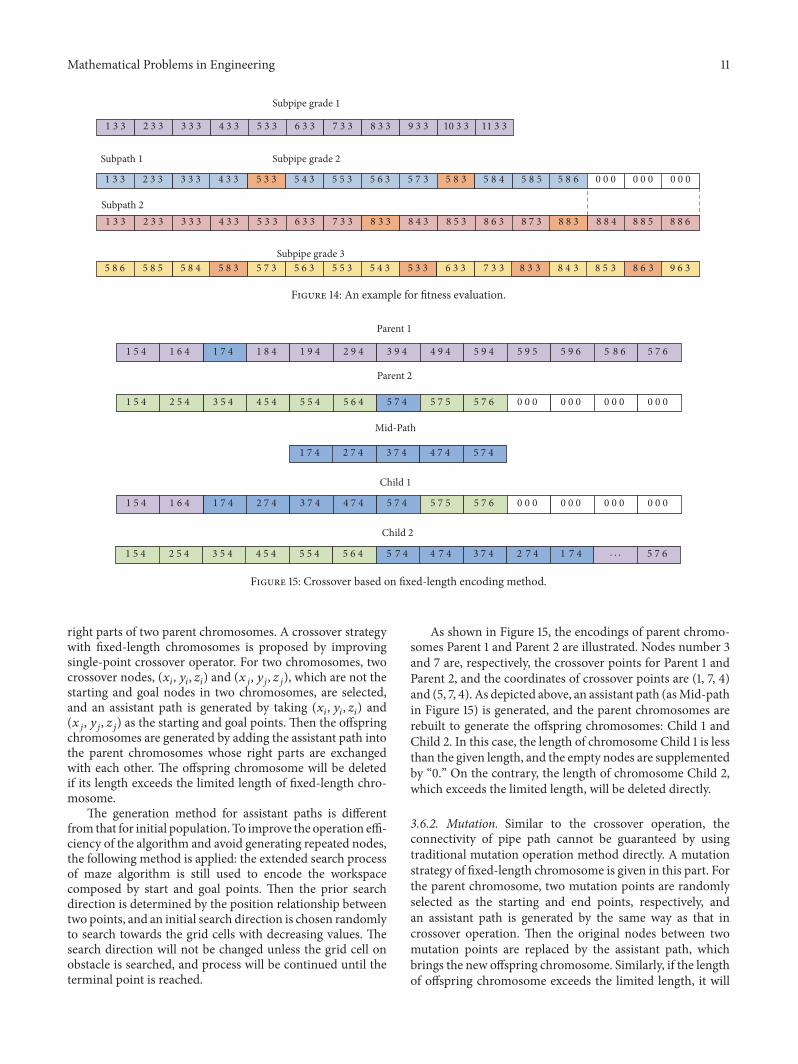
An example of pipeline with three subpipe grades isshown in Figure 14. For subpipe grade 1, the length is 11 and
the number of bends is 0; the overlapping lengthwith subpipegrade 2 and subpipe grade 3 is 8 and 4, respectively. As forsubpipe grade 2, two subpaths are included; the total length is24 and the number of bends is 4; the overlapping length withsubpipe grade 1 and subpipe grade 3 is 8 and 15, respectively.For subpipe grade 3, the length is 16 and the number of bendsis 4; the overlapping length with subpipe grade 1 and subpipegrade 2 is 4 and 15, respectively. Then, for the pipeline, thetotal length is 28 and the number of bends is 5 (3 T-junctionsincluded).
3.6. Genetic Operator. Only the pipe path chromosome,which is composed of a series of nodes with continuouscoordinates, can be regarded as a valid one. By using tra-ditional genetic operator directly in crossover and mutationoperation, the connectivity of nodes in a chromosome cannotbe guaranteed after genetic operation, which may lead to thegeneration of invalid individuals. Based on the fixed-lengthencoding method mentioned in Section 3.4, the crossoverand mutation operation method with fixed-length chromo-some is introduced by improving the traditional geneticoperator.
3.6.1. Crossover. The crossover point is selected randomlyin the traditional single-point crossover operation, and thentwo offspring individuals are generated by exchanging the
Mathematical Problems in Engineering 11
Subpipe grade 2
Subpipe grade 3
Subpipe grade 1
Subpath 1
Subpath 2
1 3 3 4 3 33 3 32 3 3 5 3 3 6 3 3 7 3 3 8 3 3 9 3 3 10 3 3 11 3 3
1 3 3 4 3 33 3 32 3 3 5 3 3 6 3 3 7 3 3 8 3 3 8 4 3 8 5 3 8 6 3 8 7 3 8 8 3 8 8 4 8 8 5 8 8 6
5 8 6 5 8 35 8 45 8 5 5 7 3 5 6 3 5 5 3 5 4 3 5 3 3 6 3 3 7 3 3 8 3 3 8 4 3 8 5 3 8 6 3 9 6 3
1 3 3 4 3 33 3 32 3 3 5 3 3 5 4 3 5 5 3 5 6 3 5 7 3 5 8 3 5 8 4 5 8 5 5 8 6 0 0 0 0 0 0 0 0 0
Figure 14: An example for fitness evaluation.
1 5 4 1 8 41 7 41 6 4 1 9 4 2 9 4 3 9 4 4 9 4 5 9 4 5 9 5 5 9 6 5 8 6 5 7 6
1 5 4 4 5 43 5 42 5 4 5 5 4 5 6 4 5 7 4 5 7 5 5 7 6 0 0 0 0 0 0 0 0 0 0 0 0
3 7 42 7 41 7 4 4 7 4 5 7 4
1 5 4 2 7 41 7 41 6 4 3 7 4 4 7 4 5 7 4 5 7 5 5 7 6 0 0 0 0 0 0 0 0 0 0 0 0
Parent 1
Parent 2
Mid-Path
Child 1
Child 2
1 5 4 4 5 43 5 42 5 4 5 5 4 5 6 4 3 7 44 7 45 7 4 2 7 4 1 7 4 5 7 6· · ·
Figure 15: Crossover based on fixed-length encoding method.
right parts of two parent chromosomes. A crossover strategywith fixed-length chromosomes is proposed by improvingsingle-point crossover operator. For two chromosomes, twocrossover nodes, (𝑥𝑖, 𝑦𝑖, 𝑧𝑖) and (𝑥𝑗, 𝑦𝑗, 𝑧𝑗), which are not thestarting and goal nodes in two chromosomes, are selected,and an assistant path is generated by taking (𝑥𝑖, 𝑦𝑖, 𝑧𝑖) and(𝑥𝑗, 𝑦𝑗, 𝑧𝑗) as the starting and goal points. Then the offspringchromosomes are generated by adding the assistant path intothe parent chromosomes whose right parts are exchangedwith each other. The offspring chromosome will be deletedif its length exceeds the limited length of fixed-length chro-mosome.
The generation method for assistant paths is differentfrom that for initial population. To improve the operation effi-ciency of the algorithm and avoid generating repeated nodes,the following method is applied: the extended search processof maze algorithm is still used to encode the workspacecomposed by start and goal points. Then the prior searchdirection is determined by the position relationship betweentwo points, and an initial search direction is chosen randomlyto search towards the grid cells with decreasing values. Thesearch direction will not be changed unless the grid cell onobstacle is searched, and process will be continued until theterminal point is reached.
As shown in Figure 15, the encodings of parent chromo-somes Parent 1 and Parent 2 are illustrated. Nodes number 3and 7 are, respectively, the crossover points for Parent 1 andParent 2, and the coordinates of crossover points are (1, 7, 4)and (5, 7, 4). As depicted above, an assistant path (asMid-pathin Figure 15) is generated, and the parent chromosomes arerebuilt to generate the offspring chromosomes: Child 1 andChild 2. In this case, the length of chromosome Child 1 is lessthan the given length, and the empty nodes are supplementedby “0.” On the contrary, the length of chromosome Child 2,which exceeds the limited length, will be deleted directly.
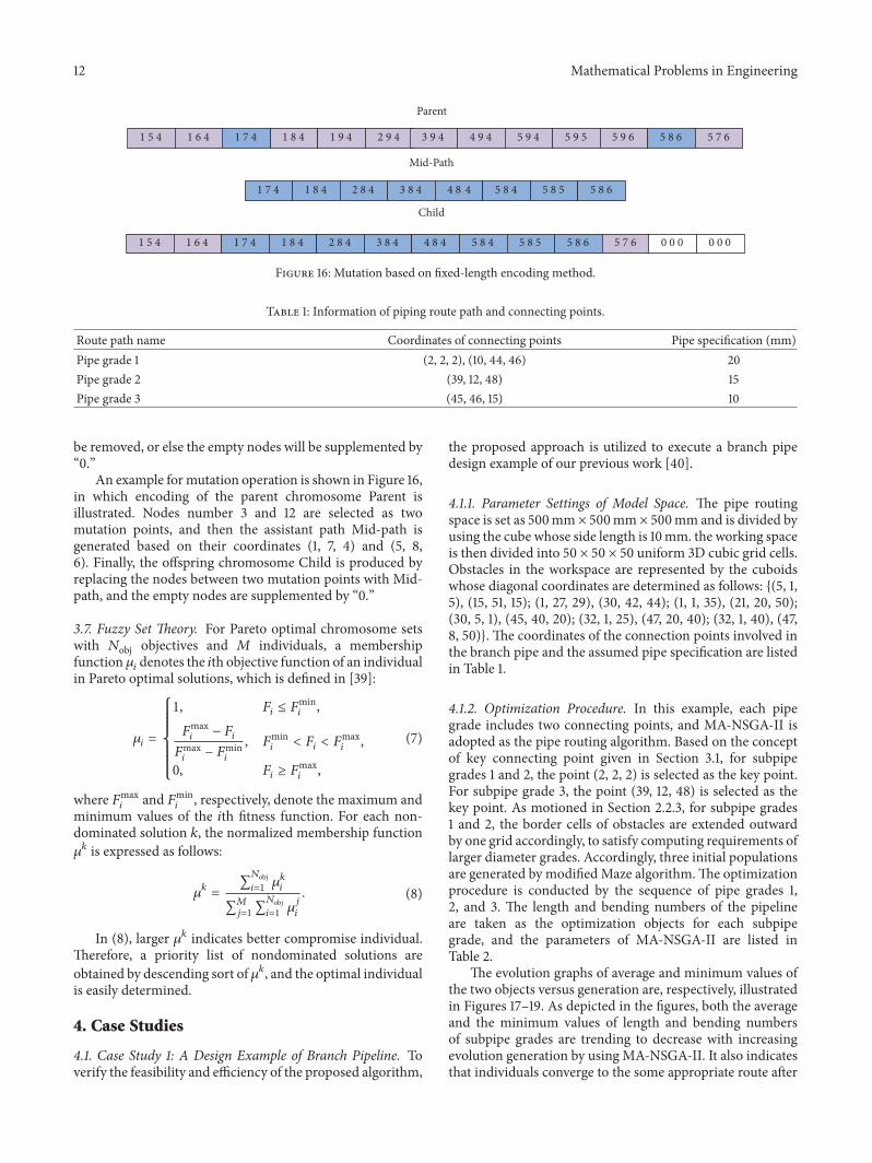
3.6.2. Mutation. Similar to the crossover operation, theconnectivity of pipe path cannot be guaranteed by usingtraditional mutation operation method directly. A mutationstrategy of fixed-length chromosome is given in this part. Forthe parent chromosome, two mutation points are randomlyselected as the starting and end points, respectively, andan assistant path is generated by the same way as that incrossover operation. Then the original nodes between twomutation points are replaced by the assistant path, whichbrings the new offspring chromosome. Similarly, if the lengthof offspring chromosome exceeds the limited length, it will
12 Mathematical Problems in Engineering
Parent
Mid-Path
Child
1 5 4 1 8 41 7 41 6 4 1 9 4 2 9 4 3 9 4 4 9 4 5 9 4 5 9 5 5 9 6 5 8 6 5 7 6
1 7 4 1 8 4 2 8 4 3 8 4 4 8 4 5 8 4 5 8 5 5 8 6
1 5 4 1 6 4 1 7 4 1 8 4 2 8 4 3 8 4 4 8 4 5 8 4 5 8 5 5 8 6 5 7 6 0 0 0 0 0 0
Figure 16: Mutation based on fixed-length encoding method.
Table 1: Information of piping route path and connecting points.
Route path name Coordinates of connecting points Pipe specification (mm)Pipe grade 1 (2, 2, 2), (10, 44, 46) 20Pipe grade 2 (39, 12, 48) 15Pipe grade 3 (45, 46, 15) 10
be removed, or else the empty nodes will be supplemented by“0.”
An example formutation operation is shown in Figure 16,in which encoding of the parent chromosome Parent isillustrated. Nodes number 3 and 12 are selected as twomutation points, and then the assistant path Mid-path isgenerated based on their coordinates (1, 7, 4) and (5, 8,6). Finally, the offspring chromosome Child is produced byreplacing the nodes between two mutation points with Mid-path, and the empty nodes are supplemented by “0.”
3.7. Fuzzy Set Theory. For Pareto optimal chromosome setswith 𝑁obj objectives and 𝑀 individuals, a membershipfunction 𝜇𝑖 denotes the 𝑖th objective function of an individualin Pareto optimal solutions, which is defined in [39]:
𝜇𝑖 ={{{{{{{{{{{
1, 𝐹𝑖 ≤ 𝐹min𝑖 ,
𝐹max𝑖 − 𝐹𝑖𝐹max𝑖 − 𝐹min
𝑖
, 𝐹min𝑖 < 𝐹𝑖 < 𝐹max
𝑖 ,0, 𝐹𝑖 ≥ 𝐹max
𝑖 ,(7)
where 𝐹max𝑖 and 𝐹min
𝑖 , respectively, denote the maximum andminimum values of the 𝑖th fitness function. For each non-dominated solution 𝑘, the normalized membership function𝜇𝑘 is expressed as follows:
𝜇𝑘 = ∑𝑁obj𝑖=1 𝜇𝑘𝑖∑𝑀𝑗=1∑𝑁obj𝑖=1 𝜇𝑗𝑖
. (8)
In (8), larger 𝜇𝑘 indicates better compromise individual.Therefore, a priority list of nondominated solutions areobtained by descending sort of 𝜇𝑘, and the optimal individualis easily determined.
4. Case Studies
4.1. Case Study 1: A Design Example of Branch Pipeline. Toverify the feasibility and efficiency of the proposed algorithm,
the proposed approach is utilized to execute a branch pipedesign example of our previous work [40].
4.1.1. Parameter Settings of Model Space. The pipe routingspace is set as 500mm × 500mm × 500mm and is divided byusing the cube whose side length is 10mm. the working spaceis then divided into 50 × 50 × 50 uniform 3D cubic grid cells.Obstacles in the workspace are represented by the cuboidswhose diagonal coordinates are determined as follows: {(5, 1,5), (15, 51, 15); (1, 27, 29), (30, 42, 44); (1, 1, 35), (21, 20, 50);(30, 5, 1), (45, 40, 20); (32, 1, 25), (47, 20, 40); (32, 1, 40), (47,8, 50)}. The coordinates of the connection points involved inthe branch pipe and the assumed pipe specification are listedin Table 1.
4.1.2. Optimization Procedure. In this example, each pipegrade includes two connecting points, and MA-NSGA-II isadopted as the pipe routing algorithm. Based on the conceptof key connecting point given in Section 3.1, for subpipegrades 1 and 2, the point (2, 2, 2) is selected as the key point.For subpipe grade 3, the point (39, 12, 48) is selected as thekey point. As motioned in Section 2.2.3, for subpipe grades1 and 2, the border cells of obstacles are extended outwardby one grid accordingly, to satisfy computing requirements oflarger diameter grades. Accordingly, three initial populationsare generated by modifiedMaze algorithm.The optimizationprocedure is conducted by the sequence of pipe grades 1,2, and 3. The length and bending numbers of the pipelineare taken as the optimization objects for each subpipegrade, and the parameters of MA-NSGA-II are listed inTable 2.
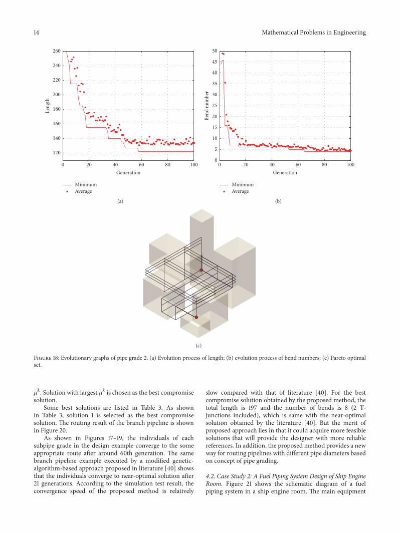
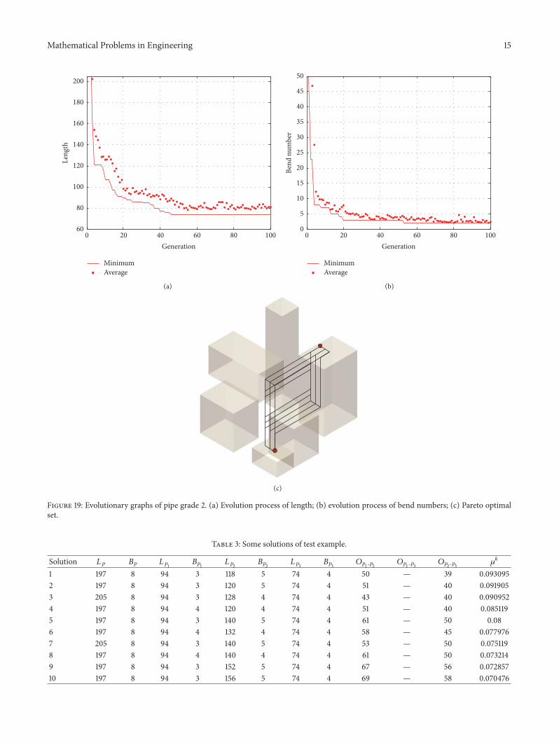
The evolution graphs of average and minimum values ofthe two objects versus generation are, respectively, illustratedin Figures 17–19. As depicted in the figures, both the averageand the minimum values of length and bending numbersof subpipe grades are trending to decrease with increasingevolution generation by using MA-NSGA-II. It also indicatesthat individuals converge to the some appropriate route after
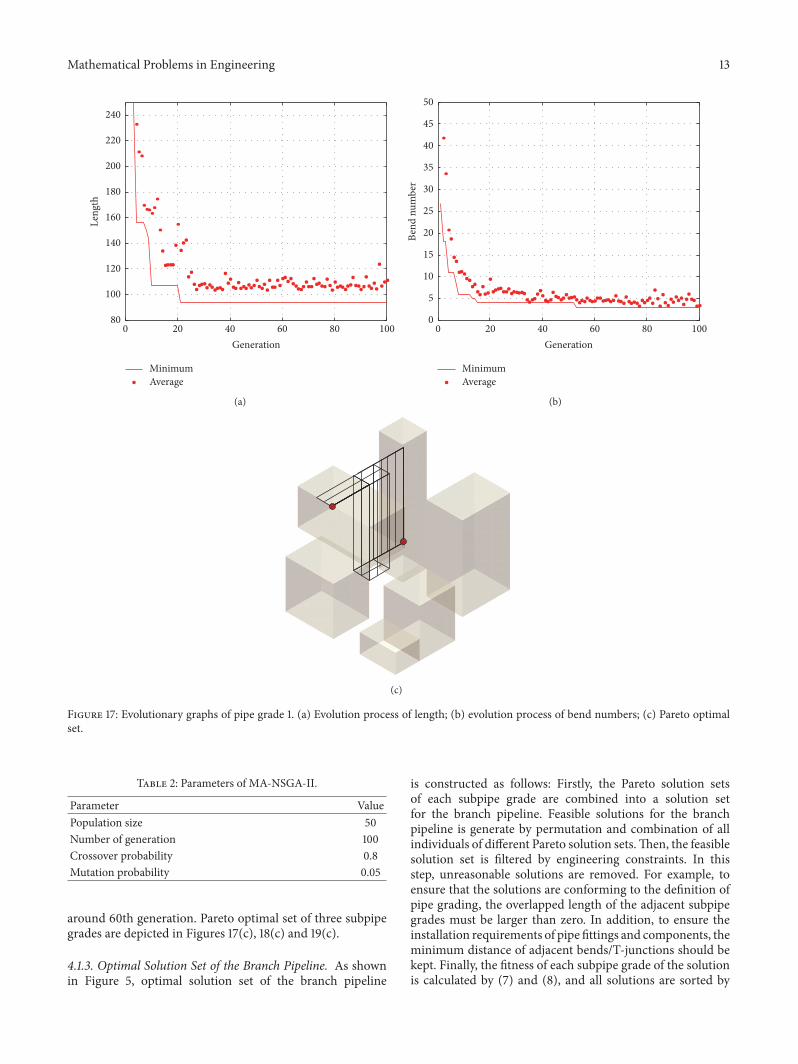
Mathematical Problems in Engineering 13
Leng
th
MinimumAverage
20 40 60 80 1000Generation
80
100
120
140
160
180
200
220
240
(a)Be
nd n
umbe
r
MinimumAverage
0
5
10
15
20
25
30
35
40
45
50
20 40 60 80 1000Generation
(b)
(c)
Figure 17: Evolutionary graphs of pipe grade 1. (a) Evolution process of length; (b) evolution process of bend numbers; (c) Pareto optimalset.
Table 2: Parameters of MA-NSGA-II.
Parameter ValuePopulation size 50Number of generation 100Crossover probability 0.8Mutation probability 0.05
around 60th generation. Pareto optimal set of three subpipegrades are depicted in Figures 17(c), 18(c) and 19(c).
4.1.3. Optimal Solution Set of the Branch Pipeline. As shownin Figure 5, optimal solution set of the branch pipeline
is constructed as follows: Firstly, the Pareto solution setsof each subpipe grade are combined into a solution setfor the branch pipeline. Feasible solutions for the branchpipeline is generate by permutation and combination of allindividuals of different Pareto solution sets.Then, the feasiblesolution set is filtered by engineering constraints. In thisstep, unreasonable solutions are removed. For example, toensure that the solutions are conforming to the definition ofpipe grading, the overlapped length of the adjacent subpipegrades must be larger than zero. In addition, to ensure theinstallation requirements of pipe fittings and components, theminimum distance of adjacent bends/T-junctions should bekept. Finally, the fitness of each subpipe grade of the solutionis calculated by (7) and (8), and all solutions are sorted by
14 Mathematical Problems in Engineering
Leng
th
MinimumAverage
20 40 60 80 1000Generation
120
140
160
180
200
220
240
260
(a)
MinimumAverage
Bend
num
ber
20 40 60 80 1000Generation
0
5
10
15
20
25
30
35
40
45
50
(b)
(c)
Figure 18: Evolutionary graphs of pipe grade 2. (a) Evolution process of length; (b) evolution process of bend numbers; (c) Pareto optimalset.
𝜇𝑘. Solution with largest 𝜇𝑘 is chosen as the best compromisesolution.
Some best solutions are listed in Table 3. As shownin Table 3, solution 1 is selected as the best compromisesolution. The routing result of the branch pipeline is shownin Figure 20.
As shown in Figures 17–19, the individuals of eachsubpipe grade in the design example converge to the someappropriate route after around 60th generation. The samebranch pipeline example executed by a modified genetic-algorithm-based approach proposed in literature [40] showsthat the individuals converge to near-optimal solution after21 generations. According to the simulation test result, theconvergence speed of the proposed method is relatively
slow compared with that of literature [40]. For the bestcompromise solution obtained by the proposed method, thetotal length is 197 and the number of bends is 8 (2 T-junctions included), which is same with the near-optimalsolution obtained by the literature [40]. But the merit ofproposed approach lies in that it could acquire more feasiblesolutions that will provide the designer with more reliablereferences. In addition, the proposed method provides a newway for routing pipelines with different pipe diameters basedon concept of pipe grading.
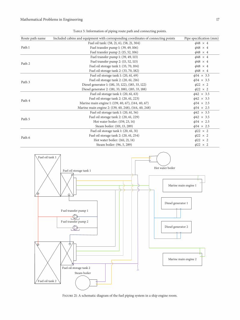
4.2. Case Study 2: A Fuel Piping System Design of Ship EngineRoom. Figure 21 shows the schematic diagram of a fuelpiping system in a ship engine room. The main equipment
Mathematical Problems in Engineering 15
20 40 60 80 1000Generation
Leng
th
MinimumAverage
60
80
100
120
140
160
180
200
(a)
MinimumAverage
Bend
num
ber
20 40 60 80 1000Generation
0
5
10
15
20
25
30
35
40
45
50
(b)
(c)
Figure 19: Evolutionary graphs of pipe grade 2. (a) Evolution process of length; (b) evolution process of bend numbers; (c) Pareto optimalset.
Table 3: Some solutions of test example.
Solution 𝐿𝑃 𝐵𝑃 𝐿𝑃1 𝐵𝑃1 𝐿𝑃2 𝐵𝑃2 𝐿𝑃3 𝐵𝑃3 𝑂𝑃1-𝑃2 𝑂𝑃1-𝑃3 𝑂𝑃2-𝑃3 𝜇𝑘1 197 8 94 3 118 5 74 4 50 — 39 0.0930952 197 8 94 3 120 5 74 4 51 — 40 0.0919053 205 8 94 3 128 4 74 4 43 — 40 0.0909524 197 8 94 4 120 4 74 4 51 — 40 0.0851195 197 8 94 3 140 5 74 4 61 — 50 0.086 197 8 94 4 132 4 74 4 58 — 45 0.0779767 205 8 94 3 140 5 74 4 53 — 50 0.0751198 197 8 94 4 140 4 74 4 61 — 50 0.0732149 197 8 94 3 152 5 74 4 67 — 56 0.07285710 197 8 94 3 156 5 74 4 69 — 58 0.070476
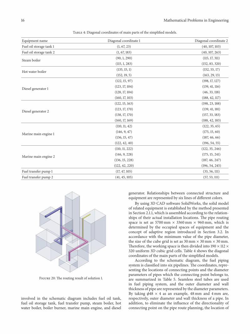
16 Mathematical Problems in Engineering
Table 4: Diagonal coordinates of main parts of the simplified models.
Equipment name Diagonal coordinate 1 Diagonal coordinate 2Fuel oil storage tank 1 (1, 67, 23) (40, 107, 103)Fuel oil storage tank 2 (1, 67, 183) (40, 107, 263)
Steam boiler (90, 1, 290) (115, 17, 311)(115, 1, 283) (152, 83, 320)
Hot water boiler (135, 15, 1) (152, 55, 17)(152, 19, 5) (163, 29, 13)
Diesel generator 1
(122, 15, 97) (198, 17, 127)(123, 17, 104) (139, 41, 116)(128, 17, 104) (46, 33, 118)(160, 17, 103) (188, 42, 117)
Diesel generator 2
(122, 15, 163) (198, 23, 188)(123, 17, 170) (139, 41, 181)(138, 17, 170) (157, 33, 183)(160, 17, 169) (188, 42, 183)
Marine main engine 1
(110, 11, 42) (122, 35, 65)(146, 9, 47) (175, 15, 60)(136, 15, 47) (187, 46, 66)(122, 42, 40) (196, 54, 55)
Marine main engine 2
(110, 11, 222) (122, 35, 246)(146, 9, 228) (175, 15, 241)(136, 15, 228) (187, 46, 247)(122, 42, 220) (196, 54, 245)
Fuel transfer pump 1 (17, 47, 105) (33, 56, 111)Fuel transfer pump 2 (41, 45, 105) (57, 53, 111)
Figure 20: The routing result of solution 1.
involved in the schematic diagram includes fuel oil tank,fuel oil storage tank, fuel transfer pump, steam boiler, hotwater boiler, boiler burner, marine main engine, and diesel
generator. Relationships between connected structure andequipment are represented by six lines of different colors.
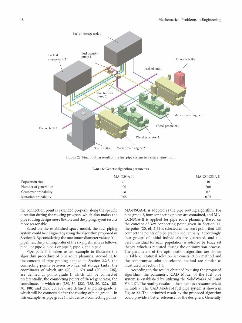
By using 3D CAD software SolidWorks, the solid modelof related equipment is established by the method presentedin Section 2.1.1, which is assembled according to the relation-ships of their actual installation locations. The pipe routingspace is set as 5700mm × 3360mm × 960mm, which isdetermined by the occupied spaces of equipment and theconcept of adaptive region introduced in Section 3.2. Inaccordance with the minimum value of the pipe diameter,the size of the cube grid is set as 30mm × 30mm × 30mm.Therefore, the working space is then divided into 190 × 112 ×320 uniform 3D cubic grid cells. Table 4 shows the diagonalcoordinates of the main parts of the simplified models.
According to the schematic diagram, the fuel pipingsystem is classified into six pipelines. The coordinates, repre-senting the locations of connecting points and the diameterparameters of pipes which the connecting point belongs to,are summarized in Table 5. Seamless steel tubes are usedin fuel piping system, and the outer diameter and wallthickness of pipe are represented by the diameter parameters.By taking 𝜙48 × 4 as an example, 48mm and 4mm are,respectively, outer diameter and wall thickness of a pipe. Inaddition, to eliminate the influence of the directionality ofconnecting point on the pipe route planning, the location of
Mathematical Problems in Engineering 17
Table 5: Information of piping route path and connecting points.
Route path name Included cabins and equipment with corresponding coordinates of connecting points Pipe specification (mm)
Path 1Fuel oil tank: (58, 21, 6), (58, 21, 304) 𝜙48 × 4Fuel transfer pump 1: (39, 49, 106) 𝜙48 × 4Fuel transfer pump 2: (15, 52, 106) 𝜙48 × 4
Path 2
Fuel transfer pump 1: (39, 49, 113) 𝜙48 × 4Fuel transfer pump 2: (15, 52, 113) 𝜙48 × 4Fuel oil storage tank 1: (33, 70, 104) 𝜙48 × 4Fuel oil storage tank 2: (33, 70, 182) 𝜙48 × 4
Path 3
Fuel oil storage tank 1: (20, 61, 69) 𝜙34 × 3.5Fuel oil storage tank 2: (20, 61, 216) 𝜙34 × 3.5
Diesel generator 1: (181, 33, 122), (185, 33, 122) 𝜙22 × 2Diesel generator 2: (181, 33, 188), (185, 33, 188) 𝜙22 × 2
Path 4
Fuel oil storage tank 1: (20, 61, 63) 𝜙42 × 3.5Fuel oil storage tank 2: (20, 61, 223) 𝜙42 × 3.5
Marine main engine 1: (139, 40, 67), (144, 40, 67) 𝜙34 × 2.5Marine main engine 2: (139, 40, 248), (144, 40, 248) 𝜙34 × 2.5
Path 5
Fuel oil storage tank 1: (20, 61, 56) 𝜙42 × 3.5Fuel oil storage tank 2: (20, 61, 229) 𝜙42 × 3.5
Hot water boiler: (159, 23, 14) 𝜙34 × 2.5Steam boiler: (101, 13, 289) 𝜙34 × 2.5
Path 6
Fuel oil storage tank 1: (20, 61, 31) 𝜙22 × 2Fuel oil storage tank 2: (20, 61, 254) 𝜙22 × 2
Hot water boiler: (161, 21, 14) 𝜙22 × 2Steam boiler: (96, 5, 289) 𝜙22 × 2
Fuel oil storage tank 1
Fuel oil storage tank 2
Fuel oil tank 1
Steam boiler
Fuel oil tank 2
Fuel transfer pump 1
Fuel transfer pump 2
Hot water boiler
Marine main engine 1
Diesel generator 1
Diesel generator 2
Marine main engine 2
Figure 21: A schematic diagram of the fuel piping system in a ship engine room.
18 Mathematical Problems in Engineering
Fuel oilstorage tank 2
Steam boiler Marine main engine 2
Diesel generator 2
Diesel generator 1
Marine main engine 1
Fuel oil tank 2
Fuel transferpump 2
Fuel oil storage tank 1
Fuel transferpump 1
Fuel oil tank 1
Hot water boiler
Figure 22: Final routing result of the fuel pipe system in a ship engine room.
Table 6: Genetic algorithm parameters.
MA-NSGA-II MA-CCNSGA-IIPopulation size 30 40Number of generation 100 200Crossover probability 0.8 0.8Mutation probability 0.05 0.05
the connection point is extended properly along the specificdirection during the routing progress, which also makes thepipe routing designmore flexible and the piping layout resultsmore reasonable.
Based on the established space model, the fuel pipingsystem could be designed by using the algorithm proposed inSection 3. By considering themaximumdiameter value of thepipelines, the planning order of the six pipelines is as follows:pipe 1 or pipe 2, pipe 4 or pipe 5, pipe 3, and pipe 6.
Pipe path 3 is taken as an example to illustrate thealgorithm procedure of pipe route planning. According tothe concept of pipe grading defined in Section 2.2.3, theconnecting points between two fuel oil storage tanks, thecoordinates of which are (20, 61, 69) and (20, 61, 216),are defined as points-grade 1, which will be connectedpreferentially; the connecting points of diesel generator, thecoordinates of which are (180, 30, 122), (185, 30, 122), (181,30, 188) and (185, 30, 188), are defined as points-grade 2,which will be connected after the routing of pipe grade 1. Inthis example, as pipe grade 1 includes two connecting points,
MA-NSGA-II is adopted as the pipe routing algorithm. Forpipe grade 2, four connecting points are contained, and MA-CCNSGA-II is applied for pipe route planning. Based onthe concept of key connecting point given in Section 3.1,the point (20, 61, 216) is selected as the start point that willconnect the points of pipe grade 2 sequentially. Accordingly,four groups of initial individuals are generated, and thebest individual for each population is selected by fuzzy settheory, which is repeated during the optimization process.The parameters of the optimization algorithm are shownin Table 6. Optimal solution set construction method andthe compromise solution selected method are similar asillustrated in Section 4.1.
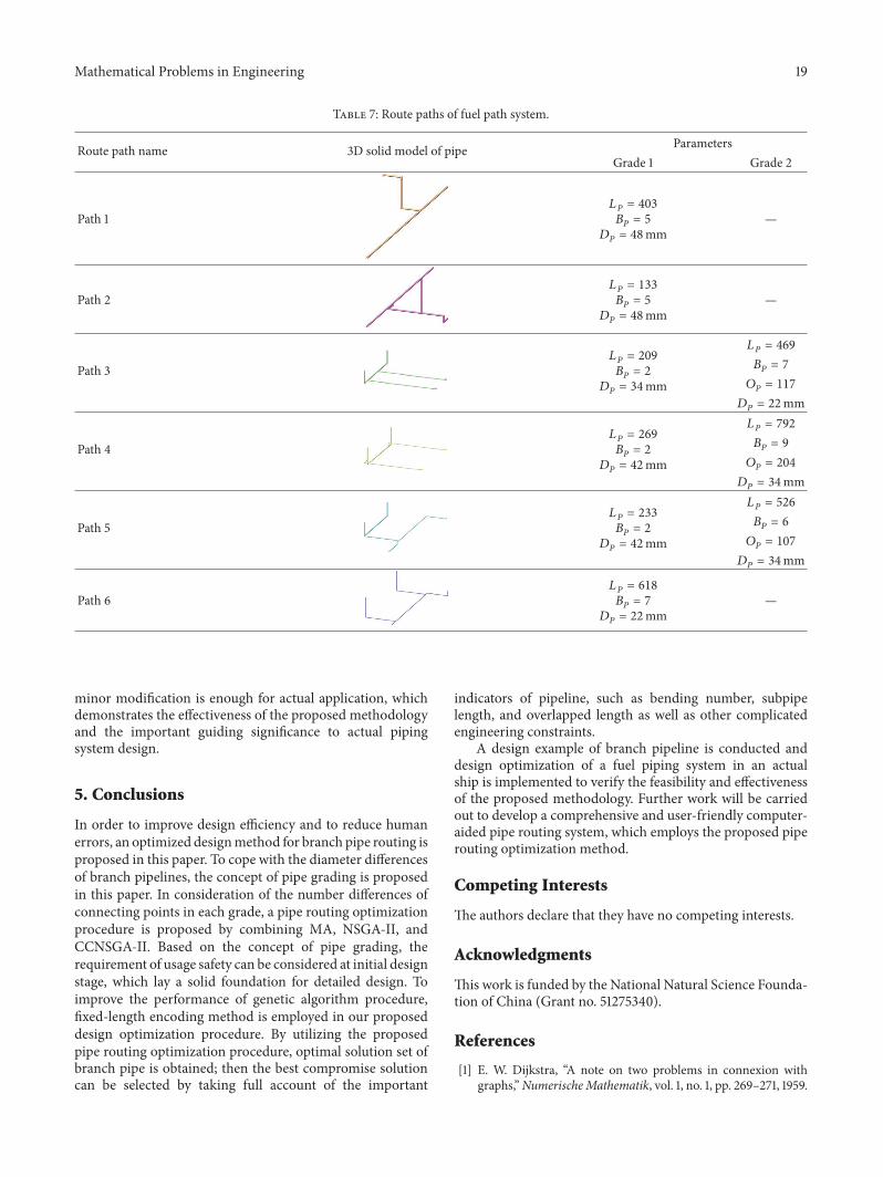
According to the results obtained by using the proposedalgorithm, the parametric CAD Model of the fuel pipesystem is established by utilizing the SolidWorks API andVB.NET.The routing results of the pipelines are summarizedin Table 7. The CAD Model of fuel pipe system is shown inFigure 22. The optimized result by the proposed algorithmcould provide a better reference for the designers. Generally,
Mathematical Problems in Engineering 19
Table 7: Route paths of fuel path system.
Route path name 3D solid model of pipe ParametersGrade 1 Grade 2
Path 1𝐿𝑃 = 403𝐵𝑃 = 5𝐷𝑃 = 48mm
—
Path 2𝐿𝑃 = 133𝐵𝑃 = 5𝐷𝑃 = 48mm
—
Path 3𝐿𝑃 = 209𝐵𝑃 = 2𝐷𝑃 = 34mm
𝐿𝑃 = 469𝐵𝑃 = 7𝑂𝑃 = 117
𝐷𝑃 = 22mm
Path 4𝐿𝑃 = 269𝐵𝑃 = 2𝐷𝑃 = 42mm
𝐿𝑃 = 792𝐵𝑃 = 9𝑂𝑃 = 204
𝐷𝑃 = 34mm
Path 5𝐿𝑃 = 233𝐵𝑃 = 2𝐷𝑃 = 42mm
𝐿𝑃 = 526𝐵𝑃 = 6𝑂𝑃 = 107
𝐷𝑃 = 34mm
Path 6𝐿𝑃 = 618𝐵𝑃 = 7𝐷𝑃 = 22mm
—
minor modification is enough for actual application, whichdemonstrates the effectiveness of the proposed methodologyand the important guiding significance to actual pipingsystem design.
5. Conclusions
In order to improve design efficiency and to reduce humanerrors, an optimized designmethod for branch pipe routing isproposed in this paper. To cope with the diameter differencesof branch pipelines, the concept of pipe grading is proposedin this paper. In consideration of the number differences ofconnecting points in each grade, a pipe routing optimizationprocedure is proposed by combining MA, NSGA-II, andCCNSGA-II. Based on the concept of pipe grading, therequirement of usage safety can be considered at initial designstage, which lay a solid foundation for detailed design. Toimprove the performance of genetic algorithm procedure,fixed-length encoding method is employed in our proposeddesign optimization procedure. By utilizing the proposedpipe routing optimization procedure, optimal solution set ofbranch pipe is obtained; then the best compromise solutioncan be selected by taking full account of the important
indicators of pipeline, such as bending number, subpipelength, and overlapped length as well as other complicatedengineering constraints.
A design example of branch pipeline is conducted anddesign optimization of a fuel piping system in an actualship is implemented to verify the feasibility and effectivenessof the proposed methodology. Further work will be carriedout to develop a comprehensive and user-friendly computer-aided pipe routing system, which employs the proposed piperouting optimization method.
Competing Interests
The authors declare that they have no competing interests.
Acknowledgments
This work is funded by the National Natural Science Founda-tion of China (Grant no. 51275340).
References
[1] E. W. Dijkstra, “A note on two problems in connexion withgraphs,”NumerischeMathematik, vol. 1, no. 1, pp. 269–271, 1959.
20 Mathematical Problems in Engineering
[2] P. E. Hart, N. J. Nilsson, and B. Raphael, “A formal basis forthe heuristic determination of minimum cost paths,” IEEETransactions on Systems Science & Cybernetics, vol. 4, no. 2, pp.100–107, 1968.
[3] C. Y. Lee, “An algorithm for path connections and its applica-tions,” IRE Transactions on Electronic Computers, vol. 10, no. 3,pp. 346–365, 1961.
[4] D. W. Hightower, “A solution to line routing problems on thecontinuous plane,” in Proceedings of the 25 Years of DAC Paperson Twenty-Five Years of Electronic Design Automation, pp. 11–34,ACM, 1988.
[5] P. W. Rourke, Development of a three-dimensional pipe routingalgorithm [Ph.D. thesis], Lehigh University, Bethlehem, Pa,USA, 1975.
[6] T. Mitsuta, Y. Kobayashi, Y. Wada et al., “A knowledge-basedapproach to routing problems in industrial plant design,” inProceedings of the 6th Internationl Workshop Vol. 1 on ExpertSystems & Their Applications, pp. 237–256, Avignon, France,1987.
[7] J. Fan,M.Ma, andX.G.Yang, “Research on automatic laying outfor external pipeline of aero-engine,” Journal of Machine Design,vol. 20, no. 7, pp. 21–23, 2003.
[8] C. E. Wang and Q. Liu, “Projection and geodesic-based piperouting algorithm,” IEEE Transactions on Automation Scienceand Engineering, vol. 8, no. 3, pp. 641–645, 2011.
[9] J. H. Holland, Adaptation in Natural and Artificial Systems,University of Michigan Press, Ann Arbor, Mich , USA, 1975.
[10] T. Ito, “Genetic algorithm approach to piping route pathplanning,” Journal of Intelligent Manufacturing, vol. 10, no. 1, pp.103–114, 1999.
[11] T. Ito, “Heuristics for route generation in pipe route planning,”in Proceedings of the 12th European Simulation Symposium (ESS’00), pp. 178–182, Hamburg, Germany, 2000.
[12] T. Ito, “Route planning wizard: basic concept and its implemen-tation,” Lecture Notes in Computer Science (including subseriesLecture Notes in Artificial Intelligence and Lecture Notes inBioinformatics), vol. 2358, pp. 547–556, 2002.
[13] X. N. Fan, Y. Lin, and Z. H. Ji, “A variable length coding geneticalgorithm to ship pipe path routing optimization in 3D space,”Shipbuilding of China, vol. 48, no. 1, pp. 82–90, 2007.
[14] S. Sandurkar and W. Chen, “GAPRUS—genetic algorithmsbased pipe routing using tessellated objects,” Computers inIndustry, vol. 38, no. 3, pp. 209–223, 1999.
[15] H. L. Wang, C. L. Zhao, W. Ch. Yan et al., “Three-dimensionalmulti-pipe route optimization based on genetic algorithms,” inKnowledge Enterprise: Intelligent Strategies in Product Design,Manufacturing, and Management, Proceedings of PROLAMAT2006, IFIP TC5 International Conference, Shanghai, China,2006, pp. 177–183, Springer, 2006.
[16] Y. Kanemoto, R. Sugawara, and M. Ohmura, “A genetic algo-rithm for the rectilinear steiner tree in 3-D VLSI layout design,”in Proceedings of the 47th Midwest Symposium on Circuits andSystems (MWSCAS ’04), pp. I-465–I-468, Hiroshima, Japan,July 2004.
[17] T. Ren, Z.-L. Zhu, G. M. Dimirovski, Z.-H. Gao, X.-H. Sun, andH. Yu, “A new pipe routing method for aero-engines based ongenetic algorithm,” Proceedings of the Institution of MechanicalEngineers, Part G: Journal of Aerospace Engineering, vol. 228, no.3, pp. 424–434, 2014.
[18] A. Colorni, M. Dorigo, V. Maniezzo et al., “Distributed opti-mization by ant colonies,” in Proceedings of the European
Conference on Artificial Life (ECAL ’91), pp. 134–142, Paris,France, 1991.
[19] M. Dorigo and L. M. Gambardella, “Ant colony system: a coop-erative learning approach to the traveling salesman problem,”IEEETransactions on Evolutionary Computation, vol. 1, no. 1, pp.53–66, 1997.
[20] X. N. Fan, Y. Lin, and Z. H. Ji, “Ship pipe routing design usingthe ACO with iterative pheromone updating,” Journal of ShipProduction, vol. 23, no. 1, pp. 36–45, 2007.
[21] X.-N. Fan, Y. Lin, and Z.-H. Ji, “Multi ant colony cooperative co-evolution for optimization of ship multi pipe parallel routing,”Journal of Shanghai Jiaotong University, vol. 43, no. 2, pp. 193–197, 2009 (Chinese).
[22] W.-Y. Jiang, Y. Lin, M. Chen, and Y.-Y. Yu, “A co-evolutionaryimproved multi-ant colony optimization for ship multiple andbranch pipe route design,” Ocean Engineering, vol. 102, pp. 63–70, 2015.
[23] Y. F. Qu, D. Jiang, G. Y. Gao, and Y. Huo, “Pipe routing approachfor aircraft engines based on ant colony optimization,” Journalof Aerospace Engineering, vol. 29, no. 3, 2016.
[24] W.-Y. Jiang, Y. Lin, M. Chen, and Y.-Y. Yu, “An ant colonyoptimization–genetic algorithm approach for ship pipe routedesign,” International Shipbuilding Progress, vol. 61, no. 3-4, pp.163–183, 2014.
[25] J. Kennedy, “Particle swarm optimization,” in Encyclopedia ofMachine Learning, pp. 760–766, Springer US, 2010.
[26] A. Asmara and U. Nienhuis, “Automatic piping system in ship,”in Proceedings of the 5th International Conference on Computerand IT Applications in the Maritime Industries, Sieca Repro(TUD ’06), pp. 269–280, Delft, The Netherlands, 2006.
[27] Q. Liu and C. E. Wang, “A discrete particle swarm optimiza-tion algorithm for rectilinear branch pipe routing,” AssemblyAutomation, vol. 31, no. 4, pp. 363–368, 2011.
[28] D. Vakil and M. R. Zargham, “An expert system for channelrouting,” in Proceedings of the 1st International Conference onIndustrial and Engineering Applications of Artificial Intelligenceand Expert Systems (IEA/AIE ’88), vol. 2, pp. 1033–1039, Tulla-homa, Tenn, USA, June 1988.
[29] J.-H. Park and R. L. Storch, “Pipe-routing algorithm develop-ment: case study of a ship engine room design,” Expert Systemswith Applications, vol. 23, no. 3, pp. 299–309, 2002.
[30] E. E. S. Calixto, P. G. Bordeira, H. T. Calazans, C. A. C. Tavares,andM. T. D. Rodriguez, “Plant design project automation usingan automatic pipe routing routine,” Computer Aided ChemicalEngineering, vol. 27, pp. 807–812, 2009.
[31] X.-Y. Shao, X.-Z. Chu, H.-B. Qiu, L. Gao, and J. Yan, “Anexpert system using rough sets theory for aided conceptualdesign of ship’s engine room automation,” Expert Systems withApplications, vol. 36, no. 2, pp. 3223–3233, 2009.
[32] J.Wu,Y. Lin, Z. S. Ji et al., “Optimal approach of ship branchpiperouting optimization based on co-evolutionary algorithm,” Shipand Ocean Engineering, vol. 37, no. 4, pp. 135–138, 2008.
[33] Q. Liu and C. Wang, “Multi-terminal pipe routing by Steinerminimal tree and particle swarm optimisation,” EnterpriseInformation Systems, vol. 6, no. 3, pp. 315–327, 2012.
[34] L. Q. Wang and Q. L. He, “Reciprocating compressor pipelinevibration analysis and engineering application,” Fluid Machin-ery, vol. 30, no. 10, pp. 28–31, 2002.
[35] K. Deb, A. Pratap, S. Agarwal, and T. Meyarivan, “A fastand elitist multiobjective genetic algorithm: NSGA-II,” IEEETransactions on Evolutionary Computation, vol. 6, no. 2, pp. 182–197, 2002.
Mathematical Problems in Engineering 21
[36] B. Dorronsoro, G. Danoy, A. J. Nebro, and P. Bouvry, “Achievingsuper-linear performance in parallel multi-objective evolution-ary algorithms by means of cooperative coevolution,” Comput-ers & Operations Research, vol. 40, no. 6, pp. 1552–1563, 2013.
[37] G. Theodosiou and N. S. Sapidis, “Information models oflayout constraints for product life-cycle management: a solid-modelling approach,” CAD Computer Aided Design, vol. 36, no.6, pp. 549–564, 2004.
[38] A. Asmara, U. Nienhuis, and R. Hekkenberg, “Approximateorthogonal simplification of 3D model ,” in Proceedings of theIEEE World Congress on Computational Intelligence (WCCI’10)—IEEE Congress on Evolutionary Computation (CEC ’10),July 2010.
[39] M. A. Abido, “Multiobjective evolutionary algorithms for elec-tric power dispatch problem,” IEEE Transactions on Evolution-ary Computation, vol. 10, no. 3, pp. 315–329, 2006.
[40] H. T. Sui and W. T. Niu, “Branch-pipe-routing approach forships using improved genetic algorithm,” Frontiers of Mechani-cal Engineering, vol. 11, no. 3, pp. 316–323, 2016.

Submit your manuscripts athttp://www.hindawi.com
Hindawi Publishing Corporationhttp://www.hindawi.com Volume 2014
MathematicsJournal of
Hindawi Publishing Corporationhttp://www.hindawi.com Volume 2014
Mathematical Problems in Engineering
Hindawi Publishing Corporationhttp://www.hindawi.com
Differential EquationsInternational Journal of
Volume 2014
Applied MathematicsJournal of
Hindawi Publishing Corporationhttp://www.hindawi.com Volume 2014
Probability and StatisticsHindawi Publishing Corporationhttp://www.hindawi.com Volume 2014
Journal of
Hindawi Publishing Corporationhttp://www.hindawi.com Volume 2014
Mathematical PhysicsAdvances in
Complex AnalysisJournal of
Hindawi Publishing Corporationhttp://www.hindawi.com Volume 2014
OptimizationJournal of
Hindawi Publishing Corporationhttp://www.hindawi.com Volume 2014
CombinatoricsHindawi Publishing Corporationhttp://www.hindawi.com Volume 2014
International Journal of
Hindawi Publishing Corporationhttp://www.hindawi.com Volume 2014
Operations ResearchAdvances in
Journal of
Hindawi Publishing Corporationhttp://www.hindawi.com Volume 2014
Function Spaces
Abstract and Applied AnalysisHindawi Publishing Corporationhttp://www.hindawi.com Volume 2014
International Journal of Mathematics and Mathematical Sciences
Hindawi Publishing Corporationhttp://www.hindawi.com Volume 2014
The Scientific World JournalHindawi Publishing Corporation http://www.hindawi.com Volume 2014
Hindawi Publishing Corporationhttp://www.hindawi.com Volume 2014
Algebra
Discrete Dynamics in Nature and Society
Hindawi Publishing Corporationhttp://www.hindawi.com Volume 2014
Hindawi Publishing Corporationhttp://www.hindawi.com Volume 2014
Decision SciencesAdvances in
Discrete MathematicsJournal of
Hindawi Publishing Corporationhttp://www.hindawi.com
Volume 2014 Hindawi Publishing Corporationhttp://www.hindawi.com Volume 2014
Stochastic AnalysisInternational Journal of