Research Article Packing Different Cuboids with Rotations ...downloads.hindawi.com/journals/ads/2014/571743.pdf · Research Article Packing Different Cuboids with Rotations and

Research ArticlePacking Different Cuboids with Rotations andSpheres into a Cuboid

Y. G. Stoyan and A. M. Chugay

Department of Mathematical Modeling and Optimal Design, Institute for Mechanical Engineering Problems,National Academy of Sciences of Ukraine, 2/10 Pozharsky Street, Kharkov 61046, Ukraine

Correspondence should be addressed to Y. G. Stoyan; [email protected]

Received 26 July 2013; Revised 27 November 2013; Accepted 9 December 2013; Published 10 March 2014

Academic Editor: S. Dempe

Copyright © 2014 Y. G. Stoyan and A. M. Chugay. This is an open access article distributed under the Creative CommonsAttribution License, which permits unrestricted use, distribution, and reproduction in any medium, provided the original work isproperly cited.

The paper considers a packing optimization problem of different spheres and cuboids into a cuboid of the minimal height.Translations and continuous rotations of cuboids are allowed. In the paper, we offer a way of construction of special functions(Φ-functions) describing how rotations can be dealt with. These functions permit us to construct the mathematical model of theproblem as a classical mathematical programming problem. Basic characteristics of themathematical model are investigated.Whensolving the problem, the characteristics allow us to apply a number of original and state-of-the-art efficient methods of local andglobal optimization. Numerical examples of packing from 20 to 300 geometric objects are given.

1. Introduction

At present, scientific research concerningmathematicalmod-eling of optimization packing problems of 3D geometricalobjects is intensively performed. The great interest to thegiven class of problems is motivated by the need of wide useof the problems both in scientific researches and applicationsin different branches of industry. Therefore, when tacklingthese classes of problems, development of fundamental basesand tools for mathematical and computer modeling is veryimportant.

A state-of-the-art review of bin packing techniques isconsidered in [1]. It should be noted that there are manypublications devoted to packing of cuboids which can berotated only through 90∘ around of all coordinate axes.

Currently, 3D packing problems of cuboids, for whichtranslations and continuous rotations are allowed, andspheres are poorly investigated.

The problem of packing nonoriented polyhedrons canbe applied in CAD system for rapid prototyping which usesselective laser sintering process of a special powder [2].Besides, the problem is applied in nanotechnologies for 3D

modeling, visual and quality analysis of structural character-istics and mechanical properties of various composite, firm,liquid, glassy materials, granulated media, and biologicalsystems [3–6]. Packing of spheres and cuboids is used tomodel heterogeneous and porous material morphologiessuch as concrete, sand, coal, porous explosives, and solidrocket propellants [7].

Also, the problem of packing nonoriented cuboids isapplied to car design [8].

Various optimization search algorithms for solving 3Dlayout problems are considered in paper [9]. In the paper,the authors notice that simulated annealing algorithms andgenetic algorithms are stochastic methods that are used in awide variety of 3D problems.

A lot of authors traditionally use either spheres orcuboids or regular oriented polyhedrons to solve 3D packingproblems. For solving problems, the Minkowski sum [10] isused.The sumcan be successfully exploited for lattice packingof geometric objects [4, 11].

Torquato and Jiao in paper [4] try to find dense packing oftetrahedra. The authors formulate the problem of generatingdense packing of polyhedra within an adaptive fundamental

Hindawi Publishing CorporationAdvances in Decision SciencesVolume 2014, Article ID 571743, 19 pageshttp://dx.doi.org/10.1155/2014/571743

2 Advances in Decision Sciences

cell subject to periodic boundary conditions as an optimiza-tion problem which they call the adaptive shrinking cellscheme.

Paper [12] presents a heuristic approach based on mixedinteger programming for solving nonstandard 3D prob-lems with additional conditions. The described approachis addressed to standard MINLP solvers exploiting linearsubstructures of the mathematical model.

The packing of 3D tetris-like items with orthogonalrotations, within a convex domain (polyhedron) with addi-tional conditions (separation planes, fixed position or ori-entation for some items, presence of “holes” within thedomain, and balancing conditions), is considered in [13].Theauthor proposes approach which is based on mixed integerlinear/nonlinear programming, from a global optimizationpoint of view with an approximate starting solution.

Article [14] is devoted to the review of modern methodsof modeling of inclusion, intersection, and contact rela-tions of geometric objects. In the given work, it is noticedthat at present one of the perspective approaches for theconstruction of adequate mathematical models of packingproblems is the method of Φ-functions. In work [15], it isshown that the method of Φ-functions allows us to improveresults of solution of packing problems of geometrical objectsdue to application of state-of-the-art nonlinear optimizationmethods.

Work [16] is devoted to the construction of Φ-functionsfor oriented (rotations are not allowed) 3D objects whosefrontiers are sphere, cuboid, cone, and cylinder. Article[17] considers the construction of the Φ-function for twoconvex oriented polytopes. In paper [18], authors developΦ-functions that handle any 2D objects whose boundaryis formed by linear segments and/or circular arcs. Con-structed Φ-functions support free translations and rotationsof objects.

In this work, we consider packing problem of spheresand cuboids. Ourmathematical model and approach supportfree translations and rotations of cuboids. In this respect,it differs from many other approaches that optimize theposition of one object at a time. In addition, the solution ofthe packing problem reduces to minimization of an objectivefunction on a multidimensional space, which can be doneby mathematical programming, while most researchers useheuristics for solving packing problems.

The considered packing problem has the following state-ment. Let there be different cuboids 𝑃

𝑖= {𝑋 = (𝑥, 𝑦, 𝑧) ∈

𝑅3

: −𝑙0

𝑖

≤ 𝑥 ≤ 𝑙0

𝑖

, −𝑤0

𝑖

≤ 𝑦 ≤ 𝑤0

𝑖

, −ℎ0

𝑖

≤ 𝑧 ≤ ℎ0

𝑖

},𝑖 ∈ 𝐼

1= {1, 2, . . . , 𝑛

1}, different spheres 𝑆

𝑗= {𝑋 = (𝑥, 𝑦, 𝑧) ∈

𝑅3

: 𝑥2

+𝑦2

+ 𝑧2

− (𝑟0

𝑗

)2

≤ 0}, 𝑗 ∈ 𝐼2= {𝑛

1+ 1, 𝑛

1+ 2, . . . , 𝑛 =

𝑛1+ 𝑛

2}, and a container (cuboid) 𝑃 = {𝑋 = (𝑥, 𝑦, 𝑧) ∈

𝑅3

: −𝑙 ≤ 𝑥 ≤ 𝑙, −𝑤 ≤ 𝑦 ≤ 𝑤, ℎ1≤ 𝑧 ≤ ℎ

2, ℎ

1> 0},

where ℎ1and ℎ

2are variables. We suppose that cuboids 𝑃

𝑖

can be both translated by vectors V𝑖= (𝑥

𝑖, 𝑦

𝑖, 𝑧

𝑖) and rotated

through angles 𝜃𝑖= (𝛼

𝑖, 𝛽

𝑖, 𝜛

𝑖), 𝑖 ∈ 𝐼

1; that is, the location

of 𝑃𝑖is defined by a vector 𝑢

𝑖= (V

𝑖, 𝜃

𝑖) ∈ 𝑅

6. Spheres 𝑆𝑗

can be translated by vectors 𝑢𝑗= (V

𝑗, 0) = (𝑥

𝑗, 𝑦

𝑗, 𝑧

𝑗, 0, 0, 0),

𝑗 ∈ 𝐼2. Thus, 𝑢

𝑖is a motion vector of geometric object 𝑂

𝑖,

where 𝑂𝑖= 𝑃

𝑖if 𝑖 ∈ 𝐼

1and 𝑂

𝑖= 𝑆

𝑖if 𝑖 ∈ 𝐼

2, 𝑖 ∈ 𝐼 = 𝐼

1∪ 𝐼

2.

Hence, a vector 𝑢 = (𝑢1, 𝑢

2, . . . , 𝑢

𝑛1

, 𝑢𝑛1+1, 𝑢

𝑛1+2, . . . , 𝑢

𝑛) ∈ 𝑅

𝜔

where 𝜔 = 6𝑛1+ 3𝑛

2determines the location of cuboids 𝑃

𝑖,

𝑖 ∈ 𝐼1and spheres 𝑆

𝑗, 𝑗 ∈ 𝐼

2, in the Euclidean 3D space 𝑅3.

In what follows, 𝑂𝑖moved by vector 𝑢

𝑖is denoted by

𝑂𝑖(𝑢

𝑖) designated as 𝑂

𝑖(𝑢

𝑖) and 𝑃 of height ℎ = ℎ

2− ℎ

1is

denoted by 𝑃(ℎ).

Basic Problem. Define a vector 𝑢 which ensures an arrange-ment of geometric objects 𝑂

𝑖, 𝑖 ∈ 𝐼, within 𝑃(ℎ), without

overlapping, so that the height ℎ of 𝑃(ℎ) will attain theminimal value.

The remainder of the paper is organized as follows.In Section 2, we describe a construction of Φ-functionsthat are used for construction of a mathematical model ofthe problem. In Section 3, the mathematical model of theproblem is constructed and basic characteristics of the modelare investigated. Section 4 defines how starting points arederived and Section 5 presents how a local extremum pointsare calculated. A smooth jump from one local maximum toone another is considered in Section 6. The construction ofpromising points is discussed in Section 7. In Section 8, wedescribe the solution algorithm. Section 9 reports the com-putational results. Some conclusions are drawn in Section 10.

2. Φ-Functions

The method of Φ-functions permits formulating adequatemathematical models of packing problems at which continu-ous rotations are allowed. The Φ-functions allow describingthe conditions of objects nonoverlapping as a collectionof inequality systems whose left-hand sides are infinitelydifferentiable functions. This permits applying state-of-the-art effective methods of local and global optimization forsolving the problem under consideration.

Definition 1. An everywhere defined and continuous func-tion Φ(u

1, u

2) : R6

→ R1 is called a Φ-function for objects𝑂1(u

1) and 𝑂

2(u

2) if the function possesses the following

characteristic properties:

Φ(u1, u

2, 𝛾

1

, 𝛾2

)

=

{{{{

{{{{

{

> 0, if 𝑂1(u

1, 𝛾

1

) ∩ 𝑂2(u

2, 𝛾

2

) = 0,

= 0, if int 𝑂1(u

1, 𝛾

1

) ∩ int 𝑂2(u

2, 𝛾

2

) = 0,

fr𝑂1(u

1, 𝛾

1

) ∩ fr𝑂2(u

2, 𝛾

2

) = 0,

< 0, if int 𝑂1(u

1, 𝛾

1

) ∩ int 𝑂2(u

2, 𝛾

2

) = 0,

(1)

where int 𝑂𝑖is the interior of𝑂

𝑖and fr𝑂

𝑖is the frontier of𝑂

𝑖.

Thus, for any location of two objects 𝑂𝑖and 𝑂

𝑗in the

Euclidean 3D space 𝑅3, the correspondingΦ-function showshow far these objects are from each other, whether they toucheach other, or whether they overlap (in the latter case, the oneshows how large the overlap is).

Consequently, in order to formulate a mathematicalmodel of the problem stated, it needs to construct Φ-functions for pairs of cuboids, cuboid and sphere, and pairsof spheres.

Advances in Decision Sciences 3

1

2

4

3

5

6

7x

y

z

Figure 1: Vertices indexing of 𝑃𝑖

(𝑢𝑖

).

2.1.Φ-Function for Two Cuboids𝑃𝑖(𝑢

𝑖) and𝑃

𝑗(𝑢

𝑗). Thearticle

[19], describes a construction of Φ-function for pairs ofconvex polytopes. As an example, the Φ-function for twocuboids is given in the article.

2.2.Φ-Function for Cuboid𝑃𝑖(𝑢

𝑖) and Sphere 𝑆

𝑗(𝑢

𝑗). Let there

be a cuboid 𝑃𝑖= {𝑋 = (𝑥, 𝑦, 𝑧) ∈ 𝑅

3

: −𝑙0

𝑖

≤ 𝑥 ≤ 𝑙0

𝑖

, −𝑤0

𝑖

≤

𝑦 ≤ 𝑤0

𝑖

, −ℎ0

𝑖

≤ 𝑧 ≤ ℎ0

𝑖

} and sphere 𝑆𝑗= {𝑋 = (𝑥, 𝑦, 𝑧) ∈

𝑅3

: 𝑥2

+ 𝑦2

+ 𝑧2

− 𝑟2

𝑗

≤ 0}. Vertex coordinates of 𝑃𝑖are

indexing as follows: 𝑉1= (𝑙

0

, 𝑤0

, ℎ0

), 𝑉2= (−𝑙

0

, 𝑤0

, ℎ0

),𝑉3= (𝑙

0

, −𝑤0

, ℎ0

),𝑉4= (−𝑙

0

, −𝑤0

, ℎ0

),𝑉5= (𝑙

0

, 𝑤0

, −ℎ0

),𝑉6=

(−𝑙0

, 𝑤0

, −ℎ0

), 𝑉7= (𝑙

0

, −𝑤0

, −ℎ0

), and 𝑉8= (−𝑙

0

, −𝑤0

, −ℎ0

)

(Figure 1).The Φ-function Φ𝑃𝑆

𝑖𝑗

(𝑢𝑖, 𝑢

𝑗) for a cuboid 𝑃

𝑖(𝑢

𝑖) and a

sphere 𝑆𝑗(𝑢

𝑗) is completely defined by an interaction of the

following subsurfaces of cuboid and sphere:

(1) a spherical surface of 𝑆𝑖(𝑢

𝑖) and facets of 𝑃

𝑗(𝑢

𝑗);


𝑖) and edges of 𝑃

𝑗(𝑢

𝑗);


𝑖) and vertices of 𝑃

𝑗(𝑢

𝑗).

If 𝑢𝑖= 0, then 0-level surface of Φ𝑃𝑆

𝑖𝑗

(0, 𝑢𝑗) has the

form depicted on Figure 2(a). It is easily seen that the 0-level surface consists of subsurfaces of planes (Figure 2(b)),cylinders (Figure 2(c)), and spheres (Figure 2(d)).

The first tangency (Figure 2(b)) form generates functions𝜒𝑖(𝑢

𝑖, 𝑢

𝑗), 𝑖 = 1, . . . , 6, which are specified as follows:

𝜒1(u

𝑖, u

𝑗) = 𝑥 (𝑢

𝑖, 𝑢

𝑗) − 𝑙

𝑖− 𝑟

𝑗,

𝜒2(u

𝑖, u

𝑗) = −𝑥 (𝑢

𝑖, 𝑢

𝑗) − 𝑙

𝑖− 𝑟

𝑗,

𝜒3(u

𝑖, u

𝑗) = 𝑦 (𝑢

𝑖, 𝑢

𝑗) − 𝑤

𝑖− 𝑟

𝑗,

𝜒4(u

𝑖, u

𝑗) = −𝑦 (𝑢

𝑖, 𝑢

𝑗) − 𝑤

𝑖− 𝑟

𝑗,

𝜒5(u

𝑖, u

𝑗) = 𝑧 (𝑢

𝑖, 𝑢

𝑗) − ℎ

𝑖− 𝑟

𝑗,

𝜒6(u

𝑖, u

𝑗) = −𝑧 (𝑢

𝑖, 𝑢

𝑗) − ℎ

𝑖− 𝑟

𝑗,

(2)

where

𝑥 (𝑢𝑖, 𝑢

𝑗) = R

𝑖(𝑥

𝑗− 𝑥

𝑖) , 𝑦 (𝑢

𝑖, 𝑢

𝑗) = R

𝑖(𝑦

𝑗− 𝑦

𝑖) ,

𝑧 (𝑢𝑖, 𝑢

𝑗) = R

𝑖(𝑧

𝑗− 𝑧

𝑖) ,

R𝑖= (

g𝑖

𝜌𝑖

q𝑖

) = (

𝑔𝑖1𝑔𝑖2𝑔𝑖3

𝑟𝑖1𝑟𝑖2𝑟𝑖3

𝑞𝑖1𝑞𝑖2𝑞𝑖3

) ,

𝑔𝑖1= cos𝛽

𝑖cos 𝛾

𝑖,

𝑔𝑖2= sin 𝛾

𝑖cos𝛼

𝑖+ cos 𝛾

𝑖sin𝛽

𝑖sin𝛼

𝑖,

𝑔𝑖3= sin 𝛾

𝑖sin𝛼

𝑖− cos 𝛾

𝑖sin𝛽

𝑖cos𝛼

𝑖,

𝑟𝑖1= − sin 𝛾

𝑖cos𝛽

𝑖,

𝑟𝑖2= cos 𝛾

𝑖cos𝛼

𝑖− sin 𝛾

𝑖sin𝛽

𝑖sin𝛼

𝑖,

𝑟𝑖3= sin𝛼

𝑖cos 𝛾

𝑖+ sin 𝛾

𝑖sin𝛽

𝑖cos𝛼

𝑖,

𝑞𝑖1= sin𝛽

𝑖, 𝑞

𝑖2= − cos𝛽

𝑖sin𝛼

𝑖,

𝑞𝑖3= cos𝛼

𝑖cos𝛽

𝑖.

(3)

It is easily verified that if at least one inequality of kind𝜒𝑙(𝑢

𝑖, 𝑢

𝑗) > 0, then𝑃

𝑖(𝑢

𝑖)∩𝑆

𝑗(𝑢

𝑗) = 0. Based on the reasoning

and relations (2), we construct the function

𝜒 (𝑢𝑖, 𝑢

𝑗) = max

𝑙=1,...,6

𝜒𝑙(𝑢

𝑖, 𝑢

𝑗) . (4)

Thus, if 𝜒(𝑢𝑖, 𝑢

𝑗) > 0 holds true, then 𝑃

𝑖(𝑢

𝑖) ∩ 𝑆

𝑗(𝑢

𝑗) = 0.

On the other hand, if 𝜒(𝑢𝑖, 𝑢

𝑗) < 0, then there can be both

𝑃𝑖(𝑢

𝑖) ∩ 𝑆

𝑗(𝑢

𝑗) = 0 and 𝑃

𝑖(𝑢

𝑖) ∩ 𝑆

𝑗(𝑢

𝑗) = 0 (see Figures 2(c) or

2(d)).The second tangency form derives cylindrical parts of

the 0-level surface of Φ𝑃𝑆

𝑖𝑗

(𝑢𝑖, 𝑢

𝑗) (see Figure 2(c)). The parts

belong to cylinders whose axes pass through edges of 𝑃𝑖(𝑢

𝑖)

and are specified by the following equations:

𝜓𝑙(𝑢

𝑖, 𝑢

𝑗) = 𝜑

2

𝑥𝑘𝑥

(𝑢𝑖, 𝑢

𝑗) + 𝜑

2

𝑦𝑘𝑦

(𝑢𝑖, 𝑢

𝑗) − 𝑟

2

𝑗

= 0,

𝑙 = 𝑘𝑥+ 2𝑘

𝑦+ 1,

𝜓𝑙(𝑢

𝑖, 𝑢

𝑗) = 𝜑

2

𝑦𝑘𝑦

(𝑢𝑖, 𝑢

𝑗) + 𝜑

2

𝑧𝑘𝑧

(𝑢𝑖, 𝑢

𝑗) − 𝑟

2

𝑗

= 0,

𝑙 = 𝑘𝑦+ 2𝑘

𝑧+ 5,

𝜓𝑙(𝑢

𝑖, 𝑢

𝑗) = 𝜑

2

𝑥𝑘𝑥

(𝑢𝑖, 𝑢

𝑗) + 𝜑

2

𝑧𝑘𝑧

(𝑢𝑖, 𝑢

𝑗) − 𝑟

2

𝑗

= 0,


𝑧+ 9,

(5)


(a) (b)

(c) (d)

Figure 2: The 0-level surface of Φ𝑃𝑆

𝑖𝑗

(0, 𝑢𝑗

).

where 𝜑𝑘𝑥

(𝑢𝑖, 𝑢

𝑗) = (−1)

𝑘𝑥𝑥(𝑢

𝑖, 𝑢

𝑗) − 𝑙

𝑖, 𝜑

𝑦𝑘𝑦

(𝑢𝑖, 𝑢

𝑗) =

(−1)𝑘𝑦𝑦(𝑢

𝑖, 𝑢

𝑗) − 𝑤

𝑖, and 𝜑

𝑧𝑘𝑧

(𝑢𝑖, 𝑢

𝑗) = (−1)

𝑘𝑧𝑧(𝑢

𝑖, 𝑢

𝑗) − ℎ

𝑖,

𝑘𝑥, 𝑘

𝑦, 𝑘

𝑧∈ {0, 1}.

In order to cut necessary parts of the cylinders, we formthe following equations of planes:

𝜒𝑙

(𝑢𝑖, 𝑢

𝑗) = 𝜑

𝑥𝑘𝑥

(𝑢𝑖, 𝑢

𝑗) + 𝜑

𝑦𝑘𝑦

(𝑢𝑖, 𝑢

𝑗) − 𝑟

𝑗= 0,


𝑦+ 1,

𝜒𝑙

(𝑢𝑖, 𝑢

𝑗) = 𝜑

𝑦𝑘𝑦

(𝑢𝑖, 𝑢

𝑗) + 𝜑

𝑧𝑘𝑧

(𝑢𝑖, 𝑢

𝑗) − 𝑟

𝑗= 0,

𝑙 = 𝑘𝑦+ 2𝑘

𝑧+ 5,

𝜒𝑙

(𝑢𝑖, 𝑢

𝑗) = 𝜑

𝑥𝑘𝑥

(𝑢𝑖, 𝑢

𝑗) + 𝜑

𝑧𝑘𝑧

(𝑢𝑖, 𝑢

𝑗) − 𝑟

𝑗= 0,


𝑧+ 9,

(6)

which are parallel to edges of 𝑃𝑖(𝑢

𝑖) and pass through pairs of

points lying at distance 𝑟𝑗from vertices 𝑉

𝑖on the extending

of edges of 𝑃𝑖(𝑢

𝑖) (see Figure 3).

z

x

y

Figure 3: The helper plane for edge (𝑉1

, 𝑉5

).


Making use of the functions 𝜓𝑙(𝑢

𝑖, 𝑢

𝑗) (5) and 𝜒

𝑙

(𝑢𝑖, 𝑢

𝑗)

(6), 𝑙 = 1, 2, . . . , 12, we form the following functions:

𝜏𝑙(𝑢

𝑖, 𝑢

𝑗) = min {𝜓

𝑙(𝑢

𝑖, 𝑢

𝑗) , 𝜒

𝑙

(𝑢𝑖, 𝑢

𝑗)} . (7)

It is evident that if at least one of the inequalities𝜏𝑙(𝑢

𝑖, 𝑢

𝑗) > 0, 𝑙 = 1, . . . , 12, holds true, then𝑃

𝑖(𝑢

𝑖)∩𝑆

𝑗(𝑢

𝑗) = 0.

The property allows us to construct the function

𝜏 (𝑢𝑖, 𝑢

𝑗) = max

𝑙=1,...,12

𝜏𝑙(𝑢

𝑖, 𝑢

𝑗) . (8)

Thus, if 𝜏(𝑢𝑖, 𝑢

𝑗) > 0, then𝑃

𝑖(𝑢

𝑖)∩𝑆

𝑗(𝑢

𝑗) = 0. On the other

hand, if 𝜏𝑙(𝑢

𝑖, 𝑢

𝑗) < 0, then there can be both 𝑃

𝑖(𝑢

𝑖) ∩ 𝑆

𝑗(𝑢

𝑗) =

0 or 𝑃𝑖(𝑢

𝑖) ∩ 𝑆

𝑗(𝑢

𝑗) = 0 (see Figure 2(d)).

The third tangency form (see Figure 2(d)) generatesspherical parts of the 0-level surface of Φ𝑃𝑆

𝑖𝑗

(𝑢𝑖, 𝑢

𝑗). The parts

belong to spheres that are formulated by equations

𝜙𝑠(𝑢

𝑖, 𝑢

𝑗)

= 𝜑2

𝑥𝑘𝑥

(𝑢𝑖, 𝑢

𝑗) + 𝜑

2

𝑦𝑘𝑦

(𝑢𝑖, 𝑢

𝑗) + 𝜑

2

𝑧𝑘𝑧

(𝑢𝑖, 𝑢

𝑗) − 𝑟

2

𝑗

= 0,

(9)

where 𝑠 = 𝑘𝑥+ 2𝑘

𝑦+ 4𝑘

𝑧+ 1, 𝑘

𝑥, 𝑘

𝑦, 𝑘

𝑧∈ {0, 1}; that is, 𝑠 =

1, 2, . . . , 8.Note that centers of the spheres coincide with vertices

𝑉𝑠, 𝑠 = 1, 2, . . . , 8, of cuboid 𝑃

𝑖(𝑢

𝑖) correspondently. We

need to extract the necessary spherical sectors of the spheres(Figure 2(d)).

To this end, we construct for each of vertices 𝑉𝑠, 𝑠 =

1, 2, . . . , 8, of 𝑃𝑖(𝑢

𝑖) three elliptic cylinders oriented by a

special way with respect to 𝑃𝑖(𝑢

𝑖) and a helper plane. Let us

consider the case in detail.Let equations of elliptic cylinders 𝐶0

𝑘

, 𝑘 = 1, 2, 3,(Figure 4) have the form

𝐶0

1

= 2𝑥2

+ 𝑦2

− 𝑟2

= 0, 𝐶0

2

= 𝑥2

+ 2𝑧2

− 𝑟2

= 0,

𝐶0

3

= 2𝑦2

+ 𝑧2

− 𝑟2

= 0.

(10)

We rotate the cylinders 𝐶0

1

, 𝐶0

2

, and 𝐶0

3

through angles𝜋/4 and −𝜋/4 round axes 𝑂𝑦, 𝑂𝑥, and 𝑂𝑧, respectively. Asa result, obtained cylinders 𝐶1

𝑡

, 𝑡 = 1, 2, . . . , 6, (see Figure 5)are specified by the equations, respectively,

𝐶1

1

= (𝑥 + 𝑧)2

+ 𝑦2

− 𝑟2

= 0,

𝐶1

2

= (𝑥 − 𝑧)2

+ 𝑦2

− 𝑟2

= 0,

𝐶1

3

= 𝑥2

+ (𝑦 + 𝑧)2

− 𝑟2

= 0,

𝐶1

4

= 𝑥2

+ (𝑧 − 𝑦)2

− 𝑟2

= 0,

𝐶1

5

= (𝑥 + 𝑦)2

+ 𝑧2

− 𝑟2

= 0,

𝐶1

6

= (𝑦 − 𝑥)2

+ 𝑧2

− 𝑟2

= 0.

(11)

It is evident that the intersections of the coordinate plane𝑥𝑂𝑦 and cylinders 𝐶1

1

, 𝐶1

2

, the coordinate plane 𝑥𝑂𝑧 and

x

y

z

Figure 4: The elliptic cylinder 𝐶0

1

.

x

y

z


1

.

cylinders𝐶1

3

,𝐶1

4

, and the coordinate plane 𝑦𝑂𝑧 and cylinders𝐶1

5

, 𝐶1

6

are circles of radius 𝑟𝑗. We rotate cylinders 𝐶1

𝑡

, 𝑗 =1, 2, . . . , 6, through the angles 𝜋/4, 3𝜋/4, 5𝜋/4, and 7𝜋/4 asfollows: cylinders 𝐶1

1

and 𝐶1

2

: we rotate round axes 𝑂𝑧 and,as a result, cylinders 𝐶2

𝑧𝑡

, 𝑡 = 1, 2, ...8, are obtained (seeFigure 6); cylinders 𝐶1

3

and 𝐶1

4

: we rotate round axes 𝑂𝑦and, as a result, cylinders 𝐶2

𝑦𝑡

, 𝑡 = 1, 2, . . . , 8, are obtained;cylinders𝐶1

5

and𝐶1

6

: we rotate round axes𝑂𝑥 and, as a result,cylinders 𝐶2

𝑥𝑡

, 𝑡 = 1, 2, . . . , 8, are obtained.Then, we translate the triple cylinders 𝐶2

𝑥𝑡

, 𝐶2

𝑦𝑡

, and 𝐶2

𝑧𝑡

,𝑡 ∈ {1, 2, . . . , 8}, by the vectors 𝑉

𝑠, 𝑠 = 1, 2, . . . , 8. Thus, we

obtain at each of the vertices 𝑉𝑠, 𝑠 = 1, 2, . . . , 8, of 𝑃

𝑖(𝑢

𝑖)


x

y

z


𝑧1

.

x

y

z


𝑧1

.

three elliptic cylinders 𝐶3

𝑥𝑡

, 𝐶3

𝑦𝑡

, and 𝐶3

𝑧𝑡

(Figure 7) which aredescribed by the following equations:

𝜙𝑠1(𝑢

𝑖, 𝑢

𝑗)=(√2𝜑

𝑥𝑘𝑥

(𝑢𝑖, 𝑢

𝑗)+𝜑

𝑦𝑘𝑦

(𝑢𝑖, 𝑢

𝑗) + 𝜑

𝑧𝑘𝑧

(𝑢𝑖, 𝑢

𝑗))

2

+ (𝜑𝑧𝑘𝑧

(𝑢𝑖, 𝑢

𝑗) − 𝜑

𝑦𝑘𝑦

(𝑢𝑖, 𝑢

𝑗))

2

− 2𝑟2

𝑗

= 0,

𝜙𝑠2(𝑢

𝑖, 𝑢

𝑗)=(𝜑

𝑥𝑘𝑥

(𝑢𝑖, 𝑢

𝑗)+√2𝜑

𝑦𝑘𝑦

(𝑢𝑖, 𝑢

𝑗) + 𝜑

𝑧𝑘𝑧

(𝑢𝑖, 𝑢

𝑗))

2

+ (𝜑𝑧𝑘𝑧

(𝑢𝑖, 𝑢

𝑗) − 𝜑

𝑥𝑘𝑥

(𝑢𝑖, 𝑢

𝑗))

2

− 2𝑟2

𝑗

= 0,

y

x

z

Figure 8: The helper plane at vertex 𝑉1

.

𝜙𝑠3(𝑢

𝑖, 𝑢

𝑗)=(𝜑

𝑥𝑘𝑥

(𝑢𝑖, 𝑢

𝑗)+𝜑

𝑦𝑘𝑦

(𝑢𝑖, 𝑢

𝑗) + √2𝜑

𝑧𝑘𝑧

(𝑢𝑖, 𝑢

𝑗))

2

+ (𝜑𝑦𝑘𝑦

(𝑢𝑖, 𝑢

𝑗) − 𝜑

𝑥𝑘𝑥

(𝑢𝑖, 𝑢

𝑗))

2

− 2𝑟2

𝑗

= 0,

(12)


𝑦+ 4𝑘

𝑧+ 1, 𝑘

𝑥, 𝑘

𝑦, 𝑘

𝑧∈ {0, 1}.

In order to cut necessary parts of the elliptic cylinders ateach of the vertices of 𝑃

𝑖(𝑢

𝑖), we form the following equations

of helper planes passing through triples of points lying atdistance 𝑟

𝑗from vertices𝑉

𝑖on the extending of edges of𝑃

𝑖(𝑢

𝑖)

(Figure 8):

𝜒𝑠(𝑢

𝑖, 𝑢

𝑗)=𝜑

𝑥𝑘𝑥

(𝑢𝑖, 𝑢

𝑗) + 𝜑

𝑦𝑘𝑦

(𝑢𝑖, 𝑢

𝑗) + 𝜑

𝑧𝑘𝑧

(𝑢𝑖, 𝑢

𝑗) − 𝑟

𝑗,

(13)


𝑦+ 4𝑘

𝑧+ 1, 𝑘

𝑥, 𝑘

𝑦, 𝑘

𝑧∈ {0, 1}.

Making use of the functions (9)–(13), we form thefunctions

𝜁𝑠(𝑢

1, 𝑢

2) = min {𝜙

𝑠(𝑢

𝑖, 𝑢

𝑗) , 𝜒

𝑠(𝑢

𝑖, 𝑢

𝑗) , 𝜙

𝑠𝑘(𝑢

𝑖, 𝑢

𝑗) ,

𝑘 = 1, 2, 3} , 𝑠 = 1, . . . , 8.

(14)

It is easily verified that if at least one of the inequalities𝜁𝑖(𝑢

𝑖, 𝑢

𝑗) > 0, 𝑠 = 1, . . . , 8, holds true, then 𝑃

𝑖(𝑢

𝑖)∩𝑆

𝑗(𝑢

𝑗) = 0.

Based on (14), we construct the function

𝜁 (𝑢𝑖, 𝑢

𝑗) = max

𝑠=1,...,8

𝜁𝑠(𝑢

𝑖, 𝑢

𝑗) . (15)

Thus, if 𝜁(𝑢𝑖, 𝑢

𝑗) > 0, then 𝑃

𝑖(𝑢

𝑖) ∩ 𝑆

𝑗(𝑢

𝑗) = 0.

Note that if at least one of inequalities either 𝜒(𝑢𝑖, 𝑢

𝑗) > 0

(4) or 𝜏(𝑢𝑖, 𝑢

𝑗) > 0 (8) or 𝜁(𝑢

𝑖, 𝑢

𝑗) > 0 (15) is satisfied, then

𝑃𝑖(𝑢

𝑖) ∩ 𝑆

𝑗(𝑢

𝑗) = 0. It allows us to construct the Φ-function

for cuboid 𝑃𝑖(𝑢

𝑖) and sphere 𝑆

𝑗(𝑢

𝑗) as follows:

Φ𝑃𝑆

𝑖𝑗

(𝑢𝑖, 𝑢

𝑗) = max {𝜒 (𝑢

𝑖, 𝑢

𝑗) , 𝜏 (𝑢

𝑖, 𝑢

𝑗) , 𝜁 (𝑢

𝑖, 𝑢

𝑗)} . (16)


2.3. Φ-Function for 𝑃𝑖and Object cl(𝑅3 \ 𝑃). It follows from

paper [19] that theΦ-function for𝑃𝑖(𝑢

𝑖) and cl(𝑅3 \𝑃) has the

form

Φ𝑃

𝑖

(𝑢𝑖) = min {𝐹

𝑘𝑗(𝑢

𝑖) , 𝑘 ∈ {1, 2, . . . , 6} , 𝑗 ∈ {1, 2, . . . , 8}} ,

(17)

where

𝐹1𝑗(𝑢

𝑖) = −𝑥

𝑖− 𝑔

𝑖𝑉𝑗+ 𝑙, 𝐹

2𝑗(𝑢

𝑖) = 𝑥

𝑖− 𝑔

𝑖𝑉𝑗+ 𝑙,

𝐹3𝑗(𝑢

𝑖) = −𝑦

𝑖− 𝑟

𝑖𝑉𝑗+ 𝑤, 𝐹

4𝑗(𝑢

𝑖) = 𝑦

𝑖− 𝑟

𝑖𝑉𝑗+ 𝑤,

𝐹5𝑗(𝑢

𝑖) = −𝑧

𝑖− 𝑞

𝑖𝑉𝑗+ ℎ

2, 𝐹

6𝑗(𝑢

𝑖) = 𝑧

𝑖− 𝑞

𝑖𝑉𝑗− ℎ

1.

(18)

2.4.Φ-Function for 𝑆𝑖andObject cl (𝑅3\𝑃). On the ground of

(5), theΦ-function for 𝑆𝑖(𝑢

𝑖) and cl(𝑅3 \𝑃) can be formulated

as

Φ𝑠

𝑖

(𝑢𝑖) = min {𝐹

𝑘(𝑢

𝑖) , 𝑘 ∈ {1, 2, . . . , 6}} , (19)

where

𝐹1(𝑢

𝑖) = −𝑥

𝑖− 𝑟

𝑖+ 𝑙, 𝐹

2(𝑢

𝑖) = 𝑥

𝑖− 𝑟

𝑖+ 𝑙,

𝐹3(𝑢

𝑖) = −𝑦

𝑖− 𝑟

𝑖+ 𝑤, 𝐹

4(𝑢

𝑖) = 𝑦

𝑖− 𝑟

𝑖+ 𝑤,

𝐹5(𝑢

𝑖) = −𝑧

𝑖− 𝑟

𝑖+ ℎ

2, 𝐹

6(𝑢

𝑖) = 𝑧

𝑖− 𝑟

𝑖− ℎ

1.

(20)

3. A Mathematical Model of the Basic Problemand Its Characteristics

In this Section, the mathematical model is constructed as atypical problem of nonsmooth mathematical programming.Characteristics of the mathematical model permit presentingthe feasible region as a union of subregions which arespecified by the inequality systems whose left-hand sides areinfinitely differentiable functions. This allows us to apply thestate-of-the-art nonlinear optimization methods to solve theproblem.

Making use of Φ-functions described in Section 2, amathematical model of the stated problem can be formulatedas

ℎ∗

= min ℎ s.t. (𝑢, ℎ) ∈ 𝑊 ⊂ 𝑅𝜔+2

, (21)

where

𝑊 = {(𝑢, ℎ) ∈ 𝑅𝜔+2

: Φ𝑃𝑃

𝑖𝑡

(𝑢𝑖, 𝑢

𝑡) ≥ 0, 0 < 𝑖 < 𝑡 ∈ 𝐼

1,

Φ𝑃𝑆

𝑖𝑗

(𝑢𝑖, 𝑢

𝑗) ≥ 0, 𝑖 ∈ 𝐼

1, 𝑗 ∈ 𝐼

2,

Φ𝑆𝑆

𝑞𝑗

(𝑢𝑞, 𝑢

𝑗) ≥ 0, 0 < 𝑞 < 𝑗 ∈ 𝐼

2,

Φ𝑃

𝑖

(𝑢𝑖, ℎ) ≥ 0, 𝑖 ∈ 𝐼

1,

Φ𝑆

𝑗

(𝑢𝑗, ℎ) ≥ 0, 𝑗 ∈ 𝐼

2}

(22)

Φ𝑃𝑃

𝑖𝑡

(𝑢𝑖, 𝑢

𝑡) ≥ 0, Φ𝑃𝑆

𝑖𝑗

(𝑢𝑖, 𝑢

𝑗) ≥ 0, and Φ𝑆𝑆

𝑖𝑗

(𝑢𝑖, 𝑢

𝑗) ≥ 0 ensure

nonoverlapping 𝑃𝑖(𝑢

𝑖) and 𝑃

𝑡(𝑢

𝑡), 𝑃

𝑖(𝑢

𝑖) and 𝑆

𝑗(𝑢

𝑗) and 𝑆

𝑖(𝑢

𝑖)

and 𝑆𝑗(𝑢

𝑗), respectively; Φ𝑃

𝑖

(𝑢𝑖, ℎ) ≥ 0 and Φ𝑆

𝑗

(𝑢𝑗, ℎ) ≥ 0

guarantee an arrangement of 𝑃𝑖(𝑢

𝑖) and 𝑆

𝑗(𝑢

𝑗) within 𝑃(ℎ),

respectively.It follows from the form of Φ-functions that the mathe-

matical model possesses the following characteristics.

(1) The feasible region𝑊 is specified by an inequality sys-tem which includes operators “max” and “min” [20].The operators contain logical constituents such as set-theoretical operations of conjunction and disjunc-tion, respectively.Thus, in inequalitiesΦ𝑃𝑃

𝑖𝑗

(𝑢𝑖, 𝑢

𝑗) ≥ 0

and Φ𝑃𝑆

𝑖𝑗

(𝑢𝑖, 𝑢

𝑗) ≥ 0, the operators “max” generate a

“union” or collection of inequality systems whereasthe operators “min” yield inequality systems. Thismeans that the feasible region 𝑊 can be alwaysrepresented by a finite union of subregions; that is,𝑊 = ⋃

𝜆

𝜉=1

𝑊𝜉, where 𝜆 = 156𝑠1 ⋅ 26𝑠2 , 156, and 26

are quantity of inequality systems in Φ𝑃𝑃

𝑖𝑡

(𝑢𝑖, 𝑢

𝑡) and

Φ𝑃𝑆

𝑖𝑗

(𝑢𝑖, 𝑢

𝑗), respectively, 𝑠

1= (1/2)𝑛

1(𝑛

1− 1), 𝑠

2=

𝑛1𝑛2.

(2) The feasible subregions𝑊𝜉are described by inequality

systems

{{{{{{{{{{{

{{{{{{{{{{{

{

𝜗

𝜉𝜙

𝑖𝑡

(𝑢𝑖, 𝑢

𝑡) ≥ 0, 0 < 𝑖 < 𝑡 ∈ 𝐼

1, 𝜙 ∈ 𝐼

𝑖𝑡,

𝜅

𝜉𝜋

𝑖𝑗

(𝑢𝑖, 𝑢

𝑗) ≥ 0, 𝑖 ∈ 𝐼

1, 𝑗 ∈ 𝐼

2, 𝜋 ∈ 𝐼

𝑖𝑗,

Φ

𝑠𝑠

𝑞𝑗

(𝑢𝑖, 𝑢

𝑗) ≥ 0, 0 < 𝑞 < 𝑗 ∈ 𝐼

2, 𝜉 ∈ 𝐽

𝜆= {1, 2, . . . , 𝜆} ,

Φ

𝑝

𝑖

(𝑢𝑖, ℎ) ≥ 0, 𝑖 ∈ 𝐼

1,

Φ

𝑠

𝑗

(𝑢𝑗, ℎ) ≥ 0, 𝑗 ∈ 𝐼

2,

(23)

where 𝜗𝜉𝜙𝑖𝑡

(𝑢𝑖, 𝑢

𝑡) ≥ 0, 𝜙 ∈ 𝐼

𝑖𝑡, and 𝜅𝜉𝜋

𝑖𝑗

(𝑢𝑖, 𝑢

𝑗) ≥

0, 𝜋 ∈ 𝐼𝑖𝑗, are inequality systems of inequality

collections which form inequalities Φ𝑃𝑃

𝑖𝑡

(𝑢𝑖, 𝑢

𝑡) ≥ 0

and Φ𝑃𝑆

𝑖𝑗

(𝑢𝑖, 𝑢

𝑗) ≥ 0. Note that functions on the left-

hand sides of the inequalities in (23) are nonlinear andinfinitely differentiable. Thus, a point (𝑢, ℎ) ∈ 𝑊 if atleast one of inequality systems (23) is satisfied.

(3) Since some subregions𝑊𝜉, 𝜉 ∈ 𝐽

𝜆, can be empty or can

be contained in other subregions, then the number 𝜎of the systems is much less than 𝜆.

(4) Some subregions of kind 𝑊𝜉may have common

points. This means that if a point 𝑢∗ is a local mini-mum with respect to𝑊

𝜉, then one has to investigate

all other subregions containing 𝑢∗ to prove that thepoint is a local minimum with respect to𝑊.

(5) Thematrix of inequality system (23) is strongly sparse.(6) The problem (21)-(22) is NP-hard [21].

The characteristics involve that a solution algorithmmustinclude the following steps: a construction of starting points,a calculation of local minima, and a nonexhaustive search oflocalminimawhich ensures a good approximation to a globalminimum.


h0

(a)

h0

(b)

Figure 9: An example of construction of a starting point.

4. Construction of Starting Points

In order to solve the problem (21)-(22), starting pointsbelonging to the feasible region 𝑊 have to be constructed.When tackling cutting and packing problems, greedy andheuristic algorithms are usually exploited to derive startingpoints [22]. The algorithms do not permit us to obtain anystarting points. This means that the algorithms significantlycontract a set of local minima to be considered. Since cuboidsare free rotated, then rules of their placement are verycomplex.This means that time expenditures when construct-ing starting points using greedy and heuristic algorithmsessentially increase in 3D space [23].The circumstances resultin a need of development of new approaches to generatestarting points.

For construction of starting points, we suggest a methodwhich assumes that all metric characteristics of objects arevariable and take values between the minimal and initialvalues. To find the starting point, a random generation ofobject placement parameters is executed. In addition, thesizes of the objects essentially diminish. After this, we solvethe problemof nonlinear programming providing an increaseof object sizes. If, as a result, the point of local maximum isobtained at which all sizes of objects reach the initial values,then the motion vector at the local maximum point andthe given height are taken as a starting point for the basicproblem.

Let us consider one of such approaches.Let sizes 𝛾

𝑖= (𝑙

𝑖, 𝑤

𝑖, ℎ

𝑖) of cuboids 𝑃

𝑖, 𝑖 ∈ 𝐼

1, and

radii 𝛾𝑗= 𝑟

𝑗of spheres 𝑆

𝑗, 𝑗 ∈ 𝐼

2, be variables. Thus,

Φ-function for objects 𝑂𝑖(𝑢

𝑖, 𝛾

𝑖) and 𝑂

𝑗(𝑢

𝑗, 𝛾

𝑗) depends on

metric characteristics of ones as well; that is, the Φ-functionhas the kind Φ

𝑖𝑗(𝑢

𝑖, 𝑢

𝑗, 𝛾

𝑖, 𝛾

𝑗).

The variables 𝛾𝑖, 𝑖 ∈ 𝐼, form a vector 𝛾 = (𝛾

1, 𝛾

2, . . . , 𝛾

𝑛) =

(𝑙1, 𝑤

1, ℎ

1, 𝑙2, 𝑤

2, ℎ

2, . . . , 𝑙

𝑛1

, 𝑤𝑛1

, ℎ𝑛1

, 𝑟𝑛1+1, 𝑟

𝑛1+2, . . . , 𝑟

𝑛) ∈ 𝑅

𝜍,where 𝜍 = 3𝑛

1+ 𝑛

2. Thus, a vector of all variables is (𝑋, ℎ) =

(𝑢, 𝛾, ℎ) ∈ 𝑅𝜇+1, where𝑋 = (𝑢, 𝛾), 𝜇 = 𝜔 + 𝜍 = 9𝑛

1+ 4𝑛

2.

We give ℎ = ℎ0 and a point 𝑋 = 𝑋∇

= (𝑢∇

, 0.1𝛾0

) =

(V∇, 𝜃∇, 0.1𝛾0) by a random way so that 𝜃∇𝑖

∈ [0, 2𝜋], V∇𝑖

∈

𝑃(ℎ0

), 𝑖 ∈ 𝐼 (Figure 9(a)). The coefficient 0.1 insures a correctconstruction of Φ-functions.

Then, taking the starting point𝑋∇, we solve the problem

𝐹 (𝛾) = max(𝑛1

∑

𝑖=1

(𝑙𝑖+ 𝑤

𝑖+ ℎ

𝑖) +

𝑛2

∑

𝑗=1

𝑟𝑗) s.t. 𝑋 ∈ Ω ⊂ 𝑅𝜇,

(24)

whereΩ = {𝑋 ∈ 𝑅

𝜇

: Φ𝑃𝑃

𝑖𝑡

(𝑢𝑖, 𝑢

𝑡, 𝛾

𝑖, 𝛾

𝑡) ≥ 0, 0 < 𝑖 < 𝑡 ∈ 𝐼

1,

Φ𝑃𝑆

𝑖𝑗

(𝑢𝑖, 𝑢

𝑗, 𝛾

𝑖, 𝛾

𝑗) ≥ 0, 𝑖 ∈ 𝐼

1, 𝑗 ∈ 𝐼

2,

Φ𝑆𝑆

𝑞𝑗

(𝑢𝑞, 𝑢

𝑗, 𝑟

𝑖, 𝑟

𝑗) ≥ 0, 0 < 𝑞 < 𝑗 ∈ 𝐼

2,

Φ𝑃

𝑖

(𝑢𝑖, 𝛾

𝑖, ℎ

0

) ≥ 0,

𝑠1𝑖(𝑤

𝑖) = 𝑙

0

𝑖

− 𝑙𝑖≥ 0,

𝑠2𝑖(𝑙𝑖) = 𝑤

0

𝑖

− 𝑤𝑖≥ 0,

𝑠3𝑖(ℎ

𝑖) = ℎ

0

𝑖

− ℎ𝑖≥ 0,

𝑙𝑖≥ 0, 𝑤

𝑖≥ 0, ℎ

𝑖≥ 0, 𝑖 ∈ 𝐼

1,

Φ𝑆

𝑗

(𝑢𝑗, 𝑟

𝑗, ℎ

0

) ≥ 0,

𝑠4𝑗(𝑟

𝑗) = 𝑟

0

𝑗

− 𝑟𝑗≥ 0, 𝑟

𝑗≥ 0, 𝑗 ∈ 𝐼

2} .

(25)

Note, that as a result of local optimization of the problem,the metric characteristics increase. In addition, they arelimited by their initial values due to the inequalities 𝑠

1𝑖(𝑤

𝑖) ≥

0, 𝑠2𝑖(𝑙𝑖) ≥ 0, 𝑠

3𝑖(ℎ

𝑖) ≥ 0, 𝑖 ∈ 𝐼

1.

As a solution result of the problem, a local maximumpoint𝑋 = (��, 𝛾) is defined (Figure 9(b)).


h0 h∗0

Figure 10: Packing corresponding to a local minimum point.

The problem (24)-(25) possesses the characteristics thatare similar to the ones of the problem (21)-(22). Furthermore,the problem (24)-(25) is master of additional properties.

(1) If𝑋 = (��, 𝛾) is a local maximum point of the problem(24)-(25) and 𝐹(𝛾) = ∑𝑛

1

𝑖=1

(𝑙𝑖+ 𝑤

𝑖+ ℎ

𝑖) + ∑

𝑛2

𝑗=1

𝑟𝑗=

∑𝑛1

𝑖=1

(𝑙0

𝑖

+𝑤0

𝑖

+ℎ0

𝑖

)+∑𝑛2

𝑗=1

𝑟0

𝑗

= 𝑑, then (��, ℎ0) ∈ 𝑊; thatis, cuboids 𝑃

𝑖(��

𝑖), 𝑖 ∈ 𝐼

1, and spheres 𝑆

𝑗(��

𝑗), 𝑗 ∈ 𝐼

2,

are packed into a cuboid 𝑃(ℎ0). This means that, inthis case, the point 𝑋 is a global maximum point ofthe problem (24)-(25).

(2) If 𝑋 = (��, 𝛾) is such that at least one of componentsof 𝛾 is strictly less matched component of 𝛾0, then𝐹(𝛾) < 𝑑 and the point 𝑋 is either a local maximumpoint or a globalmaximumpoint of the problem (24)-(25). In addition, if �� is a globalmaximumpoint, thencuboids 𝑃

𝑖(��

𝑖), 𝑖 ∈ 𝐼

1, and spheres 𝑆

𝑗(��

𝑗), 𝑗 ∈ 𝐼

2,

cannot be packed into a cuboid 𝑃(ℎ0).

Note that we always can choose ℎ = ℎ0 so that an

arrangement of geometric objects 𝑂𝑖, 𝑖 ∈ 𝐼, within 𝑃(ℎ0) is

guaranteed.

5. Calculation of Local Minima

Since we deal with a classical problem of mathematicalprogramming, then the nonlinear optimizations methodscan be used to search for local minima. The problemcharacteristics allow reducing solving the problem to solvinga sequence of the subproblems whose feasible regions arespecified by inequality systems. In addition, the left-handsides of inequalities are infinity differentiable functions; thatis, for solving the subproblems, the optimization gradientmethods can be used.

If 𝐹(𝛾) = 𝑑 (24), then (��, ℎ0) ∈ 𝑊 (22). So, the point istaken as a starting point and the problem (21)-(22) is tackled.As a result, a local minimum point (𝑢∗0, ℎ∗0) is computed(Figure 10).

Let (𝑢∗𝑖−1, ℎ∗𝑖−1) be a localminimumpoint of the problem(21)-(22) obtained after 𝑖 − 1 iterations. We take

ℎ𝑖

= (ℎ∗𝑖−1

2

− 0.25𝑗

𝑠) − (ℎ∗𝑖−1

1

+ 0.25𝑗

𝑠) ,

ℎ∗𝑖−1

> 𝑠 > 0, 𝑗 ∈ 𝑇 = {0, 1, 2, . . . , ℓ < ∞} .

(26)

Assuming 𝑗 = 0 in (26), we derive a point (𝑢∗𝑖−1, ℎ𝑖).It is evident (𝑢∗𝑖−1, ℎ𝑖) ∉ 𝑊 because of inequalities of kindΦ

𝑃

𝑡

(𝑢𝑡, ℎ

𝑖

) ≥ 0, 𝑡 ∈ 𝐼1,Φ𝑆

𝑞

(𝑢𝑞, ℎ

𝑖

) ≥ 0, 𝑞 ∈ 𝐼2, which are broken

at the point (𝑢∗𝑖−1, ℎ𝑖) (Figure 11).In order to obtain a point (��, ℎ𝑖) ∈ 𝑊, primar-

ily, we take a starting point (𝜒0, 𝑋∗𝑖−1

), where 𝜒0 =

min{Φ𝑃

𝑡

(𝑢∗𝑖−1

𝑡

, 𝛾0

𝑡

, ℎ𝑖

), 𝑡 ∈ 𝐼1, Φ

𝑆

𝑞

(𝑢∗𝑖−1

𝑞

, 𝛾0

𝑞

, ℎ0

), 𝑞 ∈ 𝐼2},

𝑋∗𝑖−1

= (𝑢∗𝑖−1

, 𝛾0

), and solve the helper problem

max𝜒 s.t. (𝜒, 𝑋) ∈ 𝐺 ⊂ 𝑅𝜇+1, (27)

where

𝐺 = { (𝜒,𝑋) ∈ 𝑅𝜇+1

: Φ𝑃𝑃

𝑖𝑡

(𝑢𝑖, 𝑢

𝑡, 𝛾

𝑖, 𝛾

𝑡)−𝜒≥0, 0<𝑖 <𝑡 ∈ 𝐼

1,

Φ𝑃𝑆

𝑖𝑗

(𝑢𝑖, 𝑢

𝑗, 𝛾

𝑖, 𝛾

𝑗) − 𝜒≥0, 𝑖∈𝐼

1, 𝑗∈𝐼

2,

Φ𝑆𝑆

𝑞𝑗

(𝑢𝑞, 𝑢

𝑗, 𝑟

𝑖, 𝑟

𝑗) − 𝜒≥0, 0<𝑞<𝑗 ∈ 𝐼

2,

Φ𝑃

𝑖

(𝑢𝑖, 𝛾

𝑖, ℎ

0

) − 𝜒 ≥ 0,

𝑠1𝑖(𝑙𝑖, 𝜒) = 𝑙

0

𝑖

− 𝑙𝑖− 𝜒 ≥ 0,

𝑠2𝑖(𝑤

𝑖, 𝜒) = 𝑤

0

𝑖

− 𝑤𝑖− 𝜒 ≥ 0,

𝑠3𝑖(ℎ

𝑖, 𝜒) = ℎ

0

𝑖

− ℎ𝑖− 𝜒 ≥ 0, 𝑖 ∈ 𝐼

1,

Φ𝑆

𝑗

(𝑢𝑗, 𝑟

𝑗, ℎ

0

) − 𝜒 ≥ 0,

𝑠4𝑗(𝑟

𝑗, 𝜒)=𝑟

0

𝑗

−𝑟𝑗−𝜒≥0, 𝑗∈𝐼

2, −𝜒≥0} .

(28)

It is easily seen that (𝜒0, 𝑋∗𝑖−1

) ∈ 𝐺.Let (𝜒∗0, 𝑋∗0

) ∈ 𝐺 be a solution of the problem (27)-(28), where 𝜒∗0 = 0 because of the inequality −𝜒 ≥ 0; thatis, (𝜒∗0, 𝑋∗0

) = (0, 𝑋∗0

) is a global minimum point.Then, taking the starting point𝑋∗0, we tackle the problem

(24)-(25) and obtain a local maximum point𝑋 = (��, 𝛾).Two cases are possible:𝐹(𝛾) = 𝑑 (Figure 11(c)) and𝐹(𝛾) <

𝑑 (Figure 12).Let 𝐹(𝛾) = 𝑑; that is, 𝑋 = (��, 𝛾) is a global maximum

of the problem (24)-(25). Hence, (��, ℎ𝑖) ∈ 𝑊. The point(��, ℎ

𝑖

) is not in the general case a local minimum point ofthe problem (21)-(22). So, taking the starting point (��, ℎ𝑖), wesolve the problem (21)-(22). As a result, a new local minimumpoint (𝑢∗𝑖, ℎ∗𝑖) is computed. Then, we assume 𝑗 = 0 in (26),take a starting point (𝜒0, 𝑋∗𝑖

) = (𝜒0

, 𝑢∗𝑖

, 𝛾0

) ∈ 𝐺 (28), andsequentially solve the problems (27)-(28), (24)-(25), (21)-(22),and so on until 𝐹(𝛾) < 𝑑 is fulfilled.

If 𝐹(𝛾) < 𝑑, we try to transit from the local maximumpoint 𝑋 to local maximum point 𝑋 so that 𝐹(𝛾) > 𝐹(𝛾)


hih∗i−1

(a)

hi

h∗i−1

(b)

hi

h∗i−1

(c)

Figure 11: An example of construction of a point (��, ℎ𝑖) ∈ 𝑊.

r0i > ri

Figure 12: Packing corresponding to 𝐹(𝛾) < 𝑑.

(see Section 6). If we cannot execute such transition, thengiving 𝑗 = 1 in (26) we take a starting point (𝜒0, 𝑋∗𝑖

) =

(𝜒0

, 𝑢∗𝑖

, 𝛾0

) ∈ 𝐺 and sequentially solve the problems (27)-(28), (24)-(25), (21)-(22), and so on until ℎ∗𝑖−1 −ℎ𝑖 < 𝜀, where𝜀 is a solution accuracy, is attained.

To calculate local extrema of the problems (21)-(22),(24)-(25), and (27)-(28), the modification of the Zoutendijkmethod of feasible directions [24] along with the concept of𝜀-active inequalities [23, 25] is used.

A computation of local extrema of the problems (21)-(22),(24)-(25), and (27)-(28) is reduced to solving a sequence ofoptimization subproblems on the feasible subregions𝑊

𝜉, 𝜉 ∈

𝐽𝜆, Ω

𝑞, 𝑞 ∈ 𝐽

𝜆, and 𝐺

𝑝, 𝑝 ∈ 𝐽

𝜆, respectively [26].

6. Transition from One LocalMaximum to Another

Since exhaustive search of all local maxima of problem (24)-(25) is theoretically possible only, then heuristic algorithms,

probabilistic approaches, or their combinations are exploitedto find approximations to a global maximum.

We offer a special approach which provides a jump froma local maximum point to another one so that the objectivefunction value may enlarge.

To this aim, we use a helper problem which maximizessizes of geometric objects at a local maximum point of theproblem (24)-(25) without restrictions on their values. Itgives us a capability to derive a vector 𝑌0 of the steepestascent of the function (24). Since restrictions of the metriccharacteristics of objects are omitted in the helper problem,then some metric characteristics increase and other onesdecrease at the point of local maximum point of the problem(24)-(25). In other words, the vector 𝑌0 shows whether thereexists “free space” which can be exploited to improve avalue of the objective function in the problem (24)-(25) andconsequently to increase sizes of objects if any.

Let 𝑋 = (��, 𝛾) = (��1, ��

2, . . . , ��

𝑛, 𝛾

1, 𝛾

2, . . . , 𝛾

𝑛) be a local

maximum point of the problem (24)-(25), ℎ = ℎ𝑖, and 𝐹(𝛾) <𝑑. Since 𝛾 = 𝛾

0, then the point (��, ℎ𝑖) ∉ 𝑊 (22). In order totransit from the point 𝑋 to the point 𝑋 so that 𝐹(𝛾) > 𝐹(𝛾),we consider the helper problem

𝐹 (𝛾∗

) = max𝐹 (𝛾) s.t 𝑋 ∈ 𝐺 ⊂ 𝑅𝜇, (29)

where

𝐺 = {𝑋 ∈ 𝑅𝜇

: Φ𝑃𝑃

𝑖𝑡

(𝑢𝑖, 𝑢

𝑡, 𝛾

𝑖, 𝛾

𝑡) ≥ 0, 𝑖 < 𝑡 ∈ 𝐼

1,

Φ𝑃𝑆

𝑖𝑗

(𝑢𝑖, 𝑢

𝑗, 𝛾

𝑖, 𝛾

𝑗) ≥ 0, 𝑖 ∈ 𝐼

1, 𝑗 ∈ 𝐼

2,

Φ𝑆𝑆

𝑞𝑗

(𝑢𝑞, 𝑢

𝑗, 𝑟

𝑞, 𝑟

𝑗) ≥ 0, 𝑞 < 𝑗 ∈ 𝐼

2,

Φ𝑃

𝑖

(𝑢𝑖, 𝛾

𝑖, ℎ

𝑘

) ≥ 0, 𝑙𝑖≥ 0,

𝑤𝑖≥ 0, ℎ

𝑖≥ 0, 𝑖 ∈ 𝐼

1,

Φ𝑆

𝑗

(𝑢𝑗, 𝑟

𝑗, ℎ

𝑘

) ≥ 0, 𝑟𝑗≥ 0, 𝑗 ∈ 𝐼

2} .

(30)


We note that the problem differs from the problem (21)-(22)by absence of restrictions

𝑠1𝑖(𝑤

𝑖) = 𝑙

0

𝑖

− 𝑙𝑖≥ 0, 𝑠

2𝑖(𝑙𝑖) = 𝑤

0

𝑖

− 𝑤𝑖≥ 0,

𝑠3𝑖(ℎ

𝑖) = ℎ

0

𝑖

− ℎ𝑖≥ 0, 𝑖 ∈ 𝐼

1,

𝑠4𝑗(𝑟

𝑗) = 𝑟

0

𝑗

− 𝑟𝑗≥ 0, 𝑗 ∈ 𝐼

2.

(31)

This means that sizes of geometric objects can take anynonnegative values.

We compute the steepest ascent vector𝑌0 at the point �� =(��, 𝛾) for the problem (29)-(30) and construct the point

𝑋]= 𝑋 + 0.5

]−1𝑌0

= 𝑋 + 𝑌0], V = 𝑉 = {1, 2, . . .} . (32)

The positive elements of the vector 𝑌0 correspondingto the direction of objects sizes change allow us to defineobjects whose sizes can be increased in the point 𝑋 oflocal maximum. Consequently, there is a “free space” inthe neighborhoods of such objects which can be used toincrease the local maximum value. Let us suppose that somecoordinates of 𝑋] satisfy the inequalities 𝑙]

𝑖

> ��𝑖, 𝑖 ∈ 𝐽

11⊂ 𝐼

1,

𝑤]𝑖

> 𝑤𝑖, 𝑖 ∈ 𝐽

12⊂ 𝐼

1, ℎ]

𝑖

> ℎ𝑖, 𝑖 ∈ 𝐽

13⊂ 𝐼

1, and 𝑟]

𝑖

> 𝑟𝑖,

𝑖 ∈ 𝐽2⊂ 𝐼

2. Let sets 𝐽

1𝑖consist of 𝑞

1𝑖, 𝑖 = 1, 2, 3, elements and

let 𝐽2consist of 𝑞

2elements.Then, 𝐽

1= 𝐽

11∪ 𝐽

12∪ 𝐽

13consists

of 𝑞1elements and 𝑞

1≤ 𝑞

11+ 𝑞

12+ 𝑞

13.

Remark 2. If 𝑌0 = 0, then there exists such 𝑚 that if V ≥ 𝑚,then𝑋]

∈ 𝐺.

We compute

𝜎0

1𝑖

= min {𝑙0𝑖

, 𝑤0

𝑖

, ℎ0

𝑖

} ,

𝜎0

2𝑖

= min {{𝑙0𝑖

, 𝑤0

𝑖

, ℎ0

𝑖

} \ {𝜎0

1𝑖

}}

𝜎0

3𝑖

= {𝑙0

𝑖

, 𝑤0

𝑖

, ℎ0

𝑖

} \ {𝜎0

1𝑖

, 𝜎0

2𝑖

} ,

��1𝑖=min {��

𝑖, 𝑤

𝑖, ℎ

𝑖} ,

��2𝑖=min {��

𝑖, 𝑤

𝑖, ℎ

1} \ {��

1𝑖} ,

��3𝑖= {��

𝑖, 𝑤

𝑖, ℎ

1} \ {��

1𝑖, ��

2𝑖} ,

𝜎𝑚

1𝑖

=min {𝑙𝑚𝑖

, 𝑤𝑚

𝑖

, ℎ𝑚

𝑖

} ,

𝜎𝑚

2𝑖

=min {𝑙𝑚𝑖

, 𝑤𝑚

𝑖

, ℎ𝑚

𝑖

} \ {𝜎𝑚

1𝑖

} ,

𝜎𝑚

3𝑖

= {𝑙𝑚

𝑖

, 𝑤𝑚

𝑖

, ℎ𝑚

𝑖

} \ {𝜎𝑚

1𝑖

, 𝜎𝑚

2𝑖

} , 𝑖 ∈ 𝐼1,

𝜌𝑚

𝑖

=√(𝑙𝑚

𝑖

)2

+ (𝑤𝑚

𝑖

)2

+ (ℎ𝑚

𝑖

)2

,

𝜌𝑖=√(��

𝑖)2

+ (𝑤𝑖)2

+ (ℎ𝑖)2

, 𝑖 ∈ 𝐼1,

𝜏𝑚

𝑖

=min {𝑙𝑚𝑖

, 𝑤𝑚

𝑖

,𝑚

𝑖

} ,

𝜏𝑖=min {��

𝑖, 𝑤

𝑖, ℎ

𝑖} , 𝑖 ∈ 𝐼

1.

(33)

Let 𝜌𝑚𝑖

> 𝜌𝑖, 𝑖 ∈ 𝐽

3⊂ 𝐼

1and 𝜏𝑚

𝑗

> 𝜏𝑗, 𝑗 ∈ 𝐽

4⊂ 𝐼

1.

On the ground of points 𝑋 and 𝑋𝑚 (see Remark 2),we derive coordinates of the vector

∘

𝑋 = (∘

𝑢1,∘

𝑢2, . . . ,

∘

𝑢𝑛,∘

𝛾1,

∘

𝛾2, . . . ,

∘

𝛾𝑛) as follows.

(1) Let 𝑖 = 𝑗 ∈ 𝐼1(𝑂

𝑖and 𝑂

𝑗are cuboids 𝑃

𝑖and 𝑃

𝑗), 𝑙0

𝑖

> ��𝑖

or𝑤0

𝑖

> 𝑤𝑖or ℎ0

𝑖

> ℎ𝑖and 𝑗 ∈ 𝐽

1; that is, at least one of metric

characteristics of𝑃𝑖does not reach the initial value and one of

metric characteristics of 𝑃𝑗is strictly greater than its value at

the point𝑋. For example, let the initial sizes of cuboids𝑃𝑖and

𝑃𝑗be 𝜎0

1𝑖

= 𝑤0

𝑖

, 𝜎02𝑖

= 𝑙0

𝑖

, and 𝜎03𝑖

= ℎ0

𝑖

and 𝜎01𝑗

= 𝑙0

𝑗

, 𝜎02𝑗

= 𝑤0

𝑗

,and 𝜎0

3𝑗

= ℎ0

𝑗

and let sizes at the point 𝑋 be ��1𝑖= 𝑤

𝑖, ��

2𝑖= ��

𝑖,

and ��3𝑖= ℎ

𝑖and ��

1𝑗= ��

𝑗, ��

2𝑗= 𝑤

𝑗, and ��

3𝑗= ℎ

𝑗, respectively.

To the points𝑋 and𝑋𝑚, there corresponds packing shown inFigure 13(a) and Figure 13(b), respectively.

Then if inequalities

��𝑡𝑗≤ 𝜎

𝑚

𝑡𝑖

, ��𝑡𝑖≤ 𝜎

𝑚

𝑡𝑗

, 𝑡 = 1, 2, 3, (34)

hold true then coordinates ∘𝑢𝑖, ∘𝑢

𝑗, ∘𝛾

𝑖and ∘𝛾

𝑗are constructed as

∘

𝑢𝑖= 𝑢

𝑚

𝑗

,∘

𝑢𝑗= 𝑢

𝑚

𝑖

,∘

𝜎𝑡𝑖= min {𝜎0

𝑡𝑖

, 𝜎𝑚

𝑡𝑗

} ,

∘

𝜎𝑡𝑗= min {𝜎𝑚

𝑡𝑖

, 𝜎0

𝑡𝑗

} , 𝑡 = 1, 2, 3,

(35)

where ∘𝜎𝑡𝑖is either

∘

𝑙𝑖or ∘𝑤

𝑖or∘

ℎ𝑖(33). This means that cuboids

𝑃𝑖and 𝑃

𝑗are “changed over” relatively their arrangement

corresponding to the point𝑋𝑚 (Figure 13(c)).If for 𝑗 ∈ 𝐽

1at least one of inequalities (34) is broken, then

∘

𝑢𝑖= 𝑢

𝑚

𝑖

,∘

𝑢𝑗= 𝑢

𝑚

𝑗

,∘

𝜎𝑡𝑖= 𝜎

𝑚

𝑡𝑖

,

∘

𝜎𝑡𝑗= 𝜎

𝑚

𝑡𝑗

, 𝑡 = 1, 2, 3.

(36)

(2) Let 𝑖 = 𝑗 ∈ 𝐼2(𝑂

𝑖and 𝑂

𝑗are spheres 𝑆

𝑖and 𝑆

𝑗), 𝑟0

𝑖

> 𝑟𝑖

and 𝑗 ∈ 𝐽2, that is radius of 𝑆

𝑖does not reach the initial value

and radius of 𝑆𝑗is strictly greater than its value at the point

𝑋. If inequalities

𝑟𝑗≤ 𝑟

𝑚

𝑖

, 𝑟𝑖≤ 𝑟

𝑚

𝑗(37)

are satisfied then coordinates ∘𝑢𝑖, ∘𝑢

𝑗, ∘𝛾

𝑖and ∘𝛾

𝑗take the form

∘

𝑢𝑖= 𝑢

𝑚

𝑗

,∘

𝑢𝑗= 𝑢

𝑚

𝑖

,∘

𝑟𝑖= min {𝑟0

𝑖

, 𝑟𝑚

𝑗

} ,

∘

𝑟𝑗= min {𝑟0

𝑗

, 𝑟𝑚

𝑖

} ,

(38)

where ∘𝛾𝑖=∘

𝑟𝑖and ∘𝛾

𝑗=∘

𝑟𝑗.

Thus, spheres 𝑆𝑖and 𝑆

𝑗are “changed over”.

If for 𝑗 ∈ 𝐽2at least one of the inequalities (37) is broken,

then∘

𝑢𝑖= 𝑢

𝑚

𝑖

,∘

𝑢𝑗= 𝑢

𝑚

𝑗

,∘

𝑟𝑖= 𝑟

𝑚

𝑖

,∘

𝑟𝑗= 𝑟

𝑚

𝑗

. (39)

(3) Let 𝑖 ∈ 𝐼1, 𝑗 ∈ 𝐼

2(𝑂

𝑖and 𝑂

𝑗are cuboid 𝑃

𝑖and

sphere 𝑆𝑗), 𝜌0

𝑖

> 𝜌𝑖, and 𝑗 ∈ 𝐽

2; that is, the radius of circle

circumscribed round 𝑃𝑖does not reach the initial value and


Pj

Pi

��1j = 𝜎01j ��2j = 𝜎02j

��1i < 𝜎01i��2i = 𝜎02i

(a)

Pj

Pi

𝜎m1j > 𝜎01j 𝜎m2j > 𝜎02j

𝜎m1i < 𝜎01i𝜎m2i > 𝜎02i

(b)

Pj

Pi

1i = 𝜎01i2i = 𝜎02i

2j = 𝜎02j1j = 𝜎01j

∘𝜎 ∘

𝜎

∘𝜎

∘𝜎

(c)

Pj

Pi

(d)

Figure 13: An example of construction of a point∘

𝑋.

radius of 𝑆𝑗is strictly greater than its value at the point 𝑋. If

inequalities

𝜌𝑖≤ 𝑟

𝑚

𝑗

, 𝑟𝑗≤ 𝜏

𝑚

𝑖(40)

are satisfied, then∘

𝑢𝑖= 𝑢

𝑚

𝑗

,∘

𝑢𝑗= 𝑢

𝑚

𝑖

,

∘

𝜎𝑡𝑖= min {𝜎0

𝑡𝑖

, 𝑟𝑚

𝑗

} , 𝑡 = 1, 2, 3,∘

𝑟𝑗= min {𝑟0

𝑗

, 𝜏𝑚

𝑖

} .

(41)

Thus, cuboid 𝑃𝑖and sphere 𝑆

𝑗are “changed over” relatively

their placement corresponding to the point𝑋𝑚.If for 𝑗 ∈ 𝐽

2at least one of the inequalities (40) is broken,

then∘

𝑢𝑖= 𝑢

𝑚

𝑖

,∘

𝑢𝑗= 𝑢

𝑚

𝑗

,∘

𝜎𝑡𝑖= 𝜎

𝑚

𝑡𝑖

,

𝑡 = 1, 2, 3,∘

𝑟𝑗= 𝑟

𝑚

𝑗

.

(42)

(4) Let 𝑖 ∈ 𝐼2, 𝑗 ∈ 𝐼

1(𝑂

𝑖and 𝑂

𝑗are sphere 𝑆

𝑖and cuboid

𝑃𝑗), 𝑟0

𝑖

> 𝑟𝑚

𝑖

, and 𝑗 ∈ 𝐽4; that is, radius of 𝑆

𝑖does not reach the

initial value and the radius of circle circumscribed round 𝑃𝑗

is strictly greater than its value at the point𝑋. If inequalities

𝑟𝑖≤ 𝜏

𝑚

𝑗

, 𝜌𝑗≤ 𝑟

𝑚

𝑖(43)

are satisfied, then∘

𝑢𝑖= 𝑢

𝑚

𝑗

,∘

𝑢𝑗= 𝑢

𝑚

𝑖

,∘

𝑟𝑖= min {𝑟0

𝑖

, 𝑟𝑚

𝑗

} ,

∘

𝜎𝑡𝑗= min {𝜎0

𝑡𝑗

, 𝑟𝑚

𝑖

} , 𝑡 = 1, 2, 3.

(44)

Thus, sphere 𝑆𝑖and cuboid 𝑃

𝑗are “changed over” relatively

their placement corresponding to the point𝑋𝑚.If for 𝑗 ∈ 𝐽

3at least one of the inequalities (43) is broken,

then we take∘

𝑢𝑖= 𝑢

𝑚

𝑖

,∘

𝑢𝑗= 𝑢

𝑚

𝑗

,∘

𝑟𝑖= 𝑟

𝑚

𝑖

,

∘

𝜎𝑡𝑗= 𝜎

𝑚

𝑡𝑗

, 𝑡 = 1, 2, 3.

(45)

Remark 3. It is easily seen that there can be∘

𝑋 = 𝑋𝑚; that is,

there exists such integer𝑁 that, if𝑚 > 𝑁, then∘

𝑋 = 𝑋𝑚.


Thus, if∘

𝑋 =𝑋𝑚, then

∘

𝑋 and 𝑋𝑚 are in attraction zonesof different local maximum points; that is, to the point

∘

𝑋

corresponds the packing of 𝑂𝑖, 𝑖 ∈ 𝐼, obtained from the

packing of 𝑂𝑖, 𝑖 ∈ 𝐼, corresponding to the point 𝑋 in which

some objects of 𝑂𝑖, 𝑖 ∈ 𝐼

1, “change over.”

Let 𝑋 be a local maximum point obtained from thestarting point

∘

𝑋.

Theorem 4. If𝑚 ≤ 𝑁, then 𝐹(𝛾) > 𝐹(𝛾).

Proof. For the sake of simplicity, let∘

𝑋 and 𝑋 differ invalues of variables 𝛾

𝑗, 𝛾

𝑖, 𝑢

𝑗, and 𝑢

𝑖only and let 𝑗 < 𝑖,

and 𝑖, 𝑗 ∈ 𝐼1; that is,

∘

𝑋 = (𝑢𝑚

1

, 𝑢𝑚

2

, . . . ,∘

𝑢𝑗, . . . ,

∘

𝑢𝑖, . . . ,

𝑢𝑚

𝑛

, 𝛾𝑚

1

, 𝛾𝑚

2

, . . . ,∘

𝛾𝑗

, . . . ,∘

𝛾𝑖

, . . . , 𝛾𝑚

𝑛

,∘

𝑟), where ∘𝑢𝑗= 𝑢

𝑚

𝑖

,∘

𝑢𝑖= 𝑢

𝑚

𝑗

,∘

𝛾𝑗

= (

∘

𝑙𝑗,∘

𝑤𝑗,

∘

ℎ𝑗), ∘𝛾

𝑖

= (

∘

𝑙𝑖,∘

𝑤𝑖,

∘

ℎ𝑖), either ∘𝑤

𝑗= min{𝑤𝑚

𝑗𝑡

, 𝜎0

𝑖

}

or ∘𝑤𝑗= 𝑤

𝑚

𝑗

, either∘

𝑙𝑗= min{𝑙𝑚

𝑗𝑡

, 𝜎0

𝑖

} or∘

𝑙𝑗= 𝑙

𝑚

𝑗

, and either∘

ℎ𝑗= min{ℎ𝑚

𝑗𝑡

, 𝜎0

𝑖

} or∘

ℎ𝑗= ℎ

𝑚

𝑗

.Note that

∘

𝑋 =𝑋𝑚 because of 𝑚 ≤ 𝑁. Hence, the point

∘

𝑋 is not in attraction zone of the local maximum point 𝑋.It follows from Remark 2 that

∘

𝑋 ∈ 𝐺; that is, the inequalitysystem {Φ

𝑖𝑗(𝑢

𝑖, 𝑢

𝑗, 𝛾

𝑖, 𝛾

𝑗) ≥ 0, 0 < 𝑖 < 𝑗 ∈ 𝐼, Φ

𝑃

𝑖

(𝑢𝑖, 𝛾

𝑖, ℎ

0

) ≥

0, 𝑤𝑖≥ 0, 𝑙

𝑖≥ 0, ℎ

𝑖≥ 0, 𝑖 ∈ 𝐼

1}, at the point

∘

𝑋 is satisfied.It follows from the relations (35) that inequalities 𝑠

1𝑖(𝑤

𝑖) =

𝑙0

𝑖

− 𝑙𝑖≥ 0, 𝑠

2𝑖(𝑙𝑖) = 𝑤

0

𝑖

− 𝑤𝑖≥ 0, 𝑠

3𝑖(ℎ

𝑖) = ℎ

0

𝑖

− ℎ𝑖≥ 0,

𝑖 ∈ 𝐼1, and 𝑠

4𝑗(𝑟𝑗) = 𝑟

0

𝑗

− 𝑟𝑗≥ 0, 𝑗 ∈ 𝐼

2, at the point

∘

𝑋, aresatisfied as well. This means that

∘

𝑋 ∈ Ω. Bearing in mind theinequalities (34), we have∑𝑛

1

𝑖=1

(

∘

𝑙𝑖+∘

𝑤𝑖+

∘

ℎ𝑖) > ∑

𝑛1

𝑖=1

(𝑙𝑖+𝑤

𝑖+ℎ

𝑖);

that is, 𝐹( ∘𝛾) > 𝐹(𝛾). It is evident that 𝐹(𝛾) > 𝐹(𝛾) if 𝑋 isa local maximum point obtained from the starting point

∘

𝑋

(see Figure 13(d)). If the number of coordinates of vectors∘

𝑋

and 𝑋 differs in the larger number of coordinates, then thetheorem holds true all the more. For the cases 2, 3, and 4, thetheorem is proved in the same way.

7. Construction of Promising Points

The theorem conditions above always ensure a jumpfrom a local maximum point to another one at whichthe objective function 𝐹(𝛾) has a more value. However,severe theorem constraints do not always allow us tofulfill such jump although the jump may execute. So,we extend a set of the starting points using points 𝑋and 𝑋

𝑚 (see Section 6). Since, in general case, localmaximum points obtained from the starting points donot guarantee an increase of values of 𝐹(𝛾), then inwhat follows the points are called promising startingones.

Let us consider a way of construction of promisingstarting points on the ground of the theorem and points𝑋 ∈𝑅𝜇 (a local maximum of the problem (24)-(25)), 𝑋𝑚

∈ 𝑅𝜇

(see (32) and Remark 2).

Firstly, making use of 𝑋 and 𝑌0 (see the problem (29)-(30)), we derive coordinates of points 𝑋𝑘, 𝜌𝑘 = (𝜌𝑘

1

, 𝜌𝑘

2

, . . . ,

𝜌𝑘

𝑛1

) and 𝜏𝑘 = (𝜏𝑘1

, 𝜏𝑘

2

, . . . , 𝜏𝑘

𝑛1

) as follows:

𝑢𝑘

𝑖

= 𝑢𝑚

𝑖

, 𝑖 ∈ 𝐼, (46)

𝑙𝑘

𝑖

= {𝑙𝑚

𝑖

if 𝑖 ∉ 𝐽11,

��𝑖+ 0.5

𝑘

𝛿 if 𝑖 ∈ 𝐽11,

𝑤𝑘

𝑖

= {𝑤𝑚

𝑖

if 𝑖 ∉ 𝐽12,

𝑤𝑖+ 0.5

𝑘

𝛿 if 𝑖 ∈ 𝐽12,

ℎ𝑘

𝑖

= {ℎ𝑚

𝑖

if 𝑖 ∉ 𝐽13,

ℎ𝑖+ 0.5

𝑘

𝛿 if 𝑖 ∈ 𝐽13,

𝑟𝑘

𝑗

= {𝑟𝑚

𝑗

if 𝑗 ∉ 𝐽2,

𝑟𝑗+ 0.5

𝑘

𝛿, if 𝑗 ∈ 𝐽2,

𝑖 ∈ 𝐼1, 𝑗 ∈ 𝐼

2,

(47)

𝜌𝑘

𝑖

= √(𝑤𝑘

𝑖

)2

+ (𝑙𝑘

𝑖

)2

+ (ℎ𝑘

𝑖

)2

, 𝑖 ∈ 𝐼1,

𝜏𝑘

𝑖

= min {𝑤𝑘

𝑖

, 𝑙𝑘

𝑖

, ℎ𝑘

𝑖

} , 𝑖 ∈ 𝐼1,

(48)

where 𝑘 ∈ 𝐾 = {1, 2, . . .}, 𝛿 = max{𝑙0𝑖

, 𝑤0

𝑖

, ℎ0

𝑖

, 𝑖 ∈ 𝐼1, 𝑟

0

𝑗

, 𝑗 ∈

𝐼2} −min{𝑙0

𝑖

, 𝑤0

𝑖

, ℎ0

𝑖

, 𝑖 ∈ 𝐼1, 𝑟

0

𝑗

, 𝑗 ∈ 𝐼2}.

It follows from (46) and (47) that a location of geometricobjects corresponding to points 𝑋𝑚 and 𝑋𝑘 coincides andmetric characteristics (sizes) may differ. Real sizes of geomet-ric objects at the points 𝑋𝑚 and 𝑋𝑘 are the same if 𝑙𝑚

𝑖

≤ ��𝑖,

𝑖 ∉ 𝐽11, 𝑤𝑚

𝑖

≤ 𝑤𝑖, 𝑖 ∉ 𝐽

12, ℎ𝑚

𝑖

≤ ℎ𝑖, 𝑖 ∉ 𝐽

13, and 𝑟𝑚

𝑖

≤ 𝑟𝑖, 𝑖 ∉ 𝐽

2.

On the other hand, if 𝑙𝑚𝑖

> ��𝑖, 𝑖 ∈ 𝐽

11,𝑤𝑚

𝑖

> 𝑤𝑖, 𝑖 ∈ 𝐽

12, ℎ𝑚

𝑖

> ℎ𝑖,

𝑖 ∈ 𝐽13, and 𝑟𝑚

𝑖

> 𝑟𝑖, 𝑖 ∈ 𝐽

2, that is, appropriate coordinates

𝑦0

𝑖

> 0, 𝑖 ∈ {𝜔1, 𝜔

2, . . . , 𝜔

𝜇} = 𝐼

𝜇, 𝜇 = 𝑞

1+ 𝑞

2, of 𝑌0, then sizes

of geometric objects 𝑂𝑖, 𝑖 ∈ 𝐼

𝜇, increase. Note that the sizes

can increase much more. In addition, the less 𝑘 in (47), themore sizes of geometric objects.

Making use of points 𝑋𝑚 and 𝑋𝑘, the point 𝑋0𝑘

=

(𝑢0𝑘

, 𝛾0𝑘

) is constructed in the same manner as the point∘

𝑋

(34)-(35) provided that, in (34), (37), (40), and (43), insteadof coordinates of 𝑋𝑚, we take coordinates of 𝑋𝑘. It is easilyseen that coordinate values of𝑋0𝑘 depend on an order of theirformation and the order influences on an effectiveness of thepromising starting point𝑋0𝑘.

In order to raise effectiveness of promising points𝑋0𝑘, 𝑘 ∈𝐾, their components are generated in order corresponding tosequences of volume increments of 𝑂

𝑖, 𝑖 ∈ 𝐼, obtained when

transiting from 𝑋 to 𝑋𝑚. Furthermore, coordinate values of𝑋

0𝑘, 𝑘 ∈ 𝐾, are derived in order corresponding to sequencesof volume increments of 𝑂

𝑖, 𝑖 ∈ 𝐼, which are equal to the

differences of initial volumes 𝑉0

𝑖

and volumes of 𝑂𝑖, 𝑖 ∈ 𝐼,

at𝑋𝑚. The sequences are constructed as follows.Let ��

𝑖and𝑉𝑚

𝑖

be volumes of objects𝑂𝑖, 𝑖 ∈ 𝐼, at the points

𝑋 and𝑋𝑚. We compute

Λ+

𝑖

= 𝑉𝑚

𝑖

− ��𝑖, Λ

−

𝑖

= 𝑉0

𝑖

− 𝑉𝑚

𝑖

, 𝑖 ∈ 𝐼. (49)


(a) (b) (c)

Figure 14: An example of construction of a promising point.

Let Λ+

𝑗

> 0, 𝑗 ∈ Υ1⊂ 𝐼, where Υ

1consists of 𝑞 elements,

andΛ−

𝑖

< 0, 𝑖 ∈ Υ2⊂ 𝐼, whereΥ

2consists of 𝑝 elements. Next,

we put Λ+

𝑗

, 𝑗 ∈ Υ1, and Λ−

𝑖

, 𝑖 ∈ Υ2, in descending order

Λ+

𝑗1

≥ Λ+

𝑗2

≥ ⋅ ⋅ ⋅ ≥ Λ+

𝑗𝑞

, (50)

Λ−

𝑖1

≥ Λ−

𝑖2

≥ ⋅ ⋅ ⋅ ≥ Λ−

𝑖𝑝

. (51)

Then, pairs of components (u0𝑘𝑖

, 𝛾0𝑘

𝑖

), 𝑖 ∈ 𝐼, of 𝑋0𝑘, 𝑘 ∈ 𝐾,are derived in the order (u0𝑘

𝑖𝑗

, 𝛾0𝑘

𝑖𝑗

), 𝑗 ∈ Υ1, (see (51)); that

is, primarily components (u0𝑘𝑖

, 𝛾0𝑘

𝑖

), 𝑖 ∈ 𝐼, correspondingto the increments of volumes Λ−

𝑗

> 0, 𝑗 ∈ Υ2, are

formed. In addition, values of the coordinates are generatedin accordance with the sequence (50); that is, at first values ofthe coordinates (u0𝑘

𝑖

, 𝛾0𝑘

𝑖

), 𝑖 ∈ 𝐼, corresponding to maximalincrements of volumes Λ+

𝑗

> 0, 𝑗 ∈ Υ1, are formed.

In other words, firstly we try to “change over” geometricobject 𝑂

𝑖1

with geometric object 𝑂𝑗1

. If such rearrangementis not possible, we try to “change over” geometric object 𝑂

𝑖1

with geometric object 𝑂𝑗2

and so on until either 𝑂𝑖1

“changeover” with 𝑂

𝑗𝑠

or 𝑂𝑗𝑡

, 𝑡 = 1, 2, . . . , 𝑞, are exhausted. After thatwe try to “change over” geometric object 𝑂

𝑖2

with geometricobject of the set 𝑂

𝑗𝑠

, 𝑠 ∈ Υ1, and so on.

Then, we put Λ+

𝑗

, 𝑗 ∈ Υ1, in ascending order

Λ+

𝑗1

≤ Λ+

𝑗2

≤ ⋅ ⋅ ⋅ ≤ Λ+

𝑗𝑞

. (52)

On the ground of the points𝑋𝑚 and𝑋𝑘, the point𝑋1𝑘

=

(𝑢1𝑘

, 𝛾1𝑘

) is formed according to the sequences (51) and (52).The point𝑋1𝑘 is derived in a way analogous to that usedwhenconstructing the point 𝑋0𝑘. Thus, the construction of 𝑋0𝑘

and 𝑋1𝑘 is distinguished by the order of formation of theircoordinate values.

Remark 5. It follows from the proof of the theorem (seeSection 6) and relations (34)–(45) that𝑋0𝑘,𝑋1𝑘

∈ Ω (25).

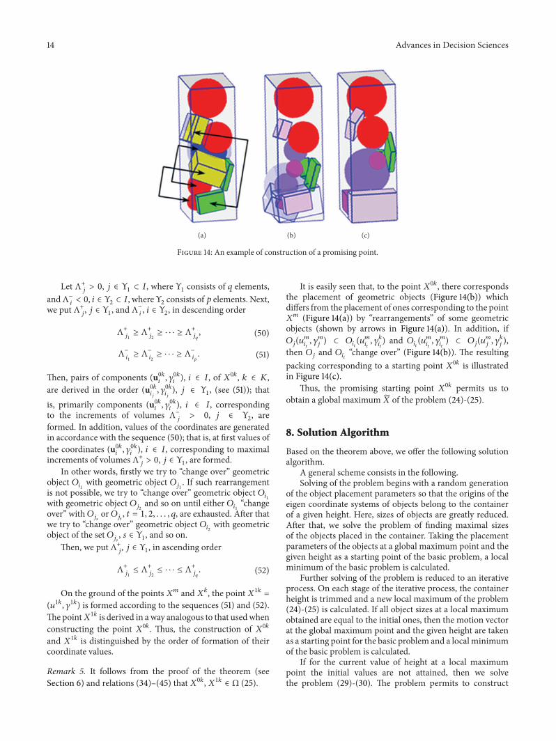
It is easily seen that, to the point 𝑋0𝑘, there correspondsthe placement of geometric objects (Figure 14(b)) whichdiffers from the placement of ones corresponding to the point𝑋

𝑚 (Figure 14(a)) by “rearrangements” of some geometricobjects (shown by arrows in Figure 14(a)). In addition, if𝑂𝑗(𝑢

𝑚

𝑖𝑡

, 𝛾𝑚

𝑗

) ⊂ 𝑂𝑖𝑡

(𝑢𝑚

𝑖𝑡

, 𝛾𝑘

𝑖𝑡

) and 𝑂𝑖𝑡

(𝑢𝑚

𝑖𝑡

, 𝛾𝑚

𝑖𝑡

) ⊂ 𝑂𝑗(𝑢

𝑚

𝑗

, 𝛾𝑘

𝑗

),then 𝑂

𝑗and 𝑂

𝑖𝑡

“change over” (Figure 14(b)). The resultingpacking corresponding to a starting point 𝑋0𝑘 is illustratedin Figure 14(c).

Thus, the promising starting point 𝑋0𝑘 permits us toobtain a global maximum𝑋 of the problem (24)-(25).

8. Solution Algorithm

Based on the theorem above, we offer the following solutionalgorithm.

A general scheme consists in the following.Solving of the problem begins with a random generation

of the object placement parameters so that the origins of theeigen coordinate systems of objects belong to the containerof a given height. Here, sizes of objects are greatly reduced.After that, we solve the problem of finding maximal sizesof the objects placed in the container. Taking the placementparameters of the objects at a global maximum point and thegiven height as a starting point of the basic problem, a localminimum of the basic problem is calculated.

Further solving of the problem is reduced to an iterativeprocess. On each stage of the iterative process, the containerheight is trimmed and a new local maximum of the problem(24)-(25) is calculated. If all object sizes at a local maximumobtained are equal to the initial ones, then the motion vectorat the global maximum point and the given height are takenas a starting point for the basic problem and a local minimumof the basic problem is calculated.

If for the current value of height at a local maximumpoint the initial values are not attained, then we solvethe problem (29)-(30). The problem permits to construct


Step 1. Take an initial value ℎ = ℎ0 so that a packing of geometric objects 𝑂𝑖

, 𝑖 ∈ 𝐼,into the cuboid 𝑃(ℎ0) is guaranteed.

Step 2. Set index 𝑖 = 0.Step 3. Give a starting point𝑋 = 𝑋∇ (see Section 4) and solve consequently the problems (24)-(25)and (21)-(22). As a result, a local minimum point (𝑢∗𝑖, ℎ∗𝑖) of the problems (21)-(22) is computed.Step 4. Repeat

BeginStep 4.1. Set index 𝑖 = 𝑖 + 1.Step 4.2. Set ℎ𝑖 = (ℎ∗𝑖−1

2

− 𝑠) − (ℎ∗𝑖−1

1

+ 𝑠) (see (26)).Step 4.3. Derive a point𝑋Δ𝑖

= (𝑢∗𝑖−1

, 𝛾0

). Take ℎ = ℎ𝑖 and a starting point (𝜒0, 𝑋Δ𝑖

) andsolve the problems (27)-(28). A global maximum point (0, 𝑋∗0

) = (0, 𝑢∗0

, 𝛾∗0

) is found.Step 4.4. Take a starting point𝑋∗0

∈ Ω and calculate a local maximum point𝑋 = (��, 𝛾) ofthe problems (24)-(25).Step 4.5. If 𝐹(𝛾) = 𝑑 then take a starting point (��, ℎ𝑖) and solve the problems (21)-(22). As aresult, a local minimum point (𝑢∗𝑖, ℎ∗𝑖) of the problems (21)-(22) is computed.End

Until 𝐹(𝛾) = 𝑑.Step 5. Set index 𝑗 = 0.Step 6. RepeatBegin

Step 6.1. Set index 𝑘 = 0.Step 6.2. RepeatBegin

Step 6.2.1. Construct a point𝑋𝑘 (46)-(47) on the ground of points 𝑌0 and𝑋.Step 6.2.2. Construct a point𝑋0𝑘

∈ Ω.Step 6.2.3. If𝑋0𝑘

= 𝑋𝑘 then take the starting point𝑋0𝑘 and solve the problems (24)-(25)

(as a result, a local maximum point 𝑋 is obtained) else go to Step 6.2.5.Step 6.2.4. If 𝐹(𝛾) > 𝐹(𝛾) and 𝐹(𝛾) < 𝑑 then take𝑋 = 𝑋 and return to Step 6.1.Step 6.2.5. If 𝐹(𝛾) > 𝐹(𝛾) and 𝐹(𝛾) = 𝑑 then go to Step 6.4.Step 6.2.6. Construct the point𝑋1𝑘

∈ Ω.Step 6.2.7. If𝑋1𝑘

= 𝑋𝑘 then take the starting point𝑋1𝑘 and solve the problems

(24)-(25) (as a result, a local maximum point 𝑋 is obtained) else go to Step 6.2.10.Step 6.2.8. If 𝐹(𝛾) > 𝐹(𝛾) and 𝐹(𝛾) < 𝑑 then take𝑋 = 𝑋 and return to Step 6.1.Step 6.2.9. If 𝐹(𝛾) > 𝐹(𝛾) and 𝐹(𝛾) = 𝑑 then go to Step 6.4.Step 6.2.10. Set 𝑘 = 𝑘 + 1.

EndUntil 𝑋0𝑘

= 𝑋 or𝑋1𝑘

= 𝑋.Step 6.4. If 𝐹(𝛾) = 𝑑 then take a starting point (��, ℎ𝑖) and solve the problems (21)-(22). As a result,a local minimum point (𝑢∗𝑖, ℎ∗𝑖) of the problems (21)-(22) is computed. Return to Step 4.Step 6.5. Set 𝑖 = 𝑖 + 1 and 𝑗 = 𝑗 + 1.Step 6.6. Set ℎ𝑖 = (ℎ∗𝑖−1

2

− 0.25𝑗

𝑠) − (ℎ∗𝑖−1

1

+ 0.25𝑗

𝑠) (see (26)).Step 6.7. Form a point𝑋Δ𝑖

= (𝑢∗𝑖−1

, 𝛾0

). Take ℎ = ℎ𝑖 and a starting point (𝜒0, 𝑋Δ𝑖

) and solve theproblems (27)-(28). As a result, a global maximum point (0, 𝑋∗0

) = (0, 𝑢∗0

, 𝛾∗0

) is found.Step 6.8. Take a starting point𝑋∗0

∈ Ω and solve the problems (24)-(25). As a result, a localmaximum point𝑋 = (��, 𝛾) is obtained.Step 6.9. If 𝐹(𝛾) = 𝑑 then return to Step 6.4.EndUntil ℎ∗𝑖−1 − ℎ𝑖 > 𝜀.Step 7. The solution process is finished. Take the point (𝑢∗𝑖−1, ℎ∗𝑖−1) as an approximation to a globalminimum of problems (21)-(22).

Algorithm 1

a vector recognizing those sizes of objects which can increase.Making use of the vector, the iterative process of searchfor promising starting points is executed. If all promisingstarting points are exhausted and the initial sizes of objectsare not attained, we enlarge the height and solve the problem(24)-(25) again and so on. The iterative process continues

until either at a local maximum point the initial sizes areobtained or an increment of the height is less than the givenaccuracy.

The last local minimum point of the basic problem istaken as an approximation to a global minimum point (seeAlgorithm 1).


(a) (b) (c)

(d) (e)

Figure 15: Examples of solution results.

Table 1: Metric characteristics of cuboids and spheres of Example 6.

𝑖 𝑙𝑖

𝑤𝑖

ℎ𝑖

𝑟𝑖

𝑃1

2 3 3 —𝑃2

2 1 3 —𝑃3

5 3 2 —𝑃4

3 0.5 3 —𝑃5

1 2 1 —𝑆6

— — — 4.4𝑆7

— — — 1.9𝑆8

— — — 5𝑆9

— — — 3.5𝑆10

— — — 2.7

9. Numerical Examples

Here, we consider examples packing from 10 to 300 geometricobjects. Results of calculations of a number of examples areavailable on http://www.datafilehost.com/d/7e0fb775. Someof the results are shown in Figure 15.

We present the following two test examples.

Example 6. Pack five cuboids and five spheres into a con-tainer with base sizes 𝑙 = 7 and 𝑤 = 5. Sizes of cuboids 𝑃

𝑖,

Table 2: Coordinates of the local minimum point of Example 6.

𝑖 𝑥𝑖

𝑦𝑖

𝑧𝑖

𝛼𝑖

𝛽𝑖

𝜛𝑖

𝑃1

5.000 1.630 4.350 4.832 3.141 6.283𝑃2

−5.680 −2.778 19.448 3.165 3.143 1.722𝑃3

3.474 0.000 11.228 3.142 3.038 1.571𝑃4

1.484 −4.479 17.854 3.159 4.767 6.296𝑃5

−1.679 2.517 21.432 6.298 3.217 6.482𝑆6

2.600 0.426 17.956 — — —𝑆7

3.867 −3.095 2.544 — — —𝑆8

−2.000 0.000 5.000 — — —𝑆9

−3.456 −1.492 13.247 — — —𝑆10

−4.282 2.292 18.215 — — —

𝑖 = 1, 2, 3, 4, 5, and spheres 𝑆𝑗, 𝑗 = 1, 2, 3, 4, 5, are given in

Table 1.

An approximation to the global minimum is equal to22.506 and is reached at the local minimum point whosecoordinates are given in Table 2.

The packing of geometric objects corresponding to thepoint is illustrated in Figure 16.

Example 7. Pack thirty cuboids into a container with basesizes 𝑙 = 14 and 𝑤 = 10. Sizes of cuboids 𝑃

𝑖are given in


Figure 16: Packing corresponding to the local minimum point(Example 6).

Figure 17: Packing corresponding to the local minimum point(Example 7).

Table 3. It should be noted that diameters of 𝑃1, 𝑃

10, and 𝑃

14

are strictly greater than diameter of the container base.

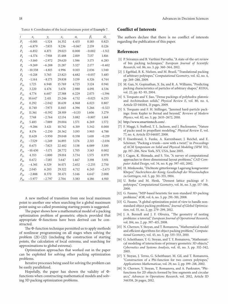
An approximation to the global minimum is equal to32.032 and is attained at the local minimum point given inTable 4.

The arrangement of geometric objects corresponding tothe local minimum point is shown in Figure 17.

All examples are calculated using Intel Core i5 (2.6Ghz)processor.

The curve shown in Figure 18 illustrates the dependenceof the runtime on 𝑛 = 𝑛

1+ 𝑛

2, where 𝑛

1= 𝑛

2.

10. Conclusions

The mathematical model describing free translations androtations of cuboids is offered.

The Φ-function for a cuboid with rotations and a sphereis constructed.

The new approach to generate random starting points isdeveloped. A random generation of object placement param-eters permits obtaining any starting points. The approach

0250500750

1000125015001750200022502500

10 20 40 60 80 100 150 300

Runt

ime (

min

)

n

Figure 18: Dependence of the runtime on 𝑛.

Table 3: Metric characteristics of cuboids of Example 7.

𝑖 𝑙𝑖

𝑤𝑖

ℎ𝑖

𝑃1

18.00 2.00 3.00𝑃2

1.00 1.50 2.00𝑃3

3.00 2.00 3.00𝑃4

1.40 3.00 2.00𝑃5

2.00 2.30 3.00𝑃6

2.50 3.00 2.00𝑃7

4.50 3.00 2.00𝑃8

2.40 4.00 4.00𝑃9

1.50 1.50 2.00𝑃10

18.00 2.00 3.00𝑃11

4.00 4.00 4.00𝑃12

3.00 3.50 1.00𝑃13

3.00 4.50 1.50𝑃14

19.00 1.00 1.00𝑃15

1.50 3.50 1.00𝑃16

3.00 1.00 2.50𝑃17

3.00 5.50 2.00𝑃18

3.00 3.20 2.00𝑃19

2.50 3.00 4.00𝑃20

3.00 4.00 4.00𝑃21

2.50 3.00 2.00𝑃22

3.00 5.00 2.00𝑃23

3.00 2.00 3.00𝑃24

3.50 3.00 2.00𝑃25

4.00 3.00 3.00𝑃26

2.50 3.00 2.00𝑃27

4.50 3.00 2.00𝑃28

2.00 2.00 2.00𝑃29

1.50 1.50 2.00𝑃30

3.00 1.70 2.00

simplifies significantly the construction of starting points andpossesses universal properties; that is, we do not need toanalyze space forms (shapes) of geometric objects and todevelop their placement rules.


Table 4: Coordinates of the local minimum point of Example 7.

𝑖 𝑥𝑖

𝑦𝑖

𝑧𝑖

𝛼𝑖

𝛽𝑖

𝜛𝑖

𝑃1

−0.001 −1.524 14.352 4.455 0.185 0.825𝑃2

−6.879 −7.833 9.236 −0.067 2.159 0.126𝑃3

−6.852 6.871 29.023 0.000 −0.002 −1.512𝑃4

−4.374 −7.918 15.488 2.819 7.137 1.816𝑃5

−3.160 −2.972 29.620 1.586 3.175 6.283𝑃6

−9.269 −6.208 21.287 3.327 2.177 −0.402𝑃7

−10.558 −4.815 4.996 0.103 2.036 1.540𝑃8

−0.218 5.765 23.823 4.682 −0.057 5.485𝑃9

−1.144 −8.175 29.838 3.159 4.326 4.744𝑃10

1.725 6.948 15.769 4.725 3.124 0.941𝑃11

3.220 4.476 5.678 2.980 4.091 4.536𝑃12

4.774 6.607 27.388 6.229 2.075 −1.596𝑃13

10.647 2.411 25.246 4.732 −0.025 6.253𝑃14

0.292 −2.042 18.639 4.968 6.023 0.807𝑃15

11.740 −7.973 11.845 4.396 5.266 −0.323𝑃16

11.361 −0.592 28.919 −0.133 1.606 3.279𝑃17

7.748 −2.764 12.134 3.082 −0.807 1.168𝑃18

5.483 −7.889 29.004 1.571 6.269 1.572𝑃19

−9.286 3.421 10.742 6.319 5.342 0.000𝑃20

8.176 −2.250 20.362 3.193 3.903 4.788𝑃21

11.628 −5.950 29.048 0.338 1.618 −0.219𝑃22

−7.529 −1.249 14.893 3.176 2.515 −2.036𝑃23

0.675 −7.823 22.402 3.138 6.089 3.100𝑃24

−10.430 −3.171 28.772 1.705 3.143 0.002𝑃25

4.353 −1.800 29.014 3.734 1.575 0.979𝑃26

0.672 −7.185 5.647 1.467 3.198 3.931𝑃27

−4.361 6.529 16.071 2.652 −2.255 2.750𝑃28

2.045 6.203 29.322 4.712 6.243 −2.673𝑃29

−2.888 8.370 30.471 5.146 4.647 2.008𝑃30

−5.977 −2.797 2.704 3.383 4.186 4.910

A new method of transition from one local maximumpoint to another one when searching for a global maximumpoint using so-called promising starting points is suggested.

The paper shows how a mathematical model of a packingoptimization problem of geometric objects provided thatappropriate Φ-functions have been derived can be con-structed.

TheΦ-function technique permitted us to apply methodsof nonlinear programming on all stages when solving theproblem (21)-(22) (including the construction of startingpoints, the calculation of local extrema, and searching forapproximations to global extrema).

Optimization approaches that worked out in the papercan be exploited for solving other packing optimizationproblems.

Iterative processes being used for solving the problem canbe easily parallelized.

Hopefully, the paper has shown the validity of Φ-functions when constructing mathematical models and solv-ing 3D packing optimization problems.

Conflict of Interests

The authors declare that there is no conflict of interestsregarding the publication of this paper.

References

[1] P. Sriramya and B. Varthini Parvatha, “A state-of-the-art reviewof bin packing techniques,” European Journal of ScientificResearch, vol. 86, no. 3, pp. 360–364, 2012.

[2] J. Egeblad, B. K. Nielsen, and M. Brazil, “Translational packingof arbitrary polytopes,” Computational Geometry, vol. 42, no. 4,pp. 269–288, 2009.

[3] M. Gan, N. Gopinathan, X. Jia, and R. A. Williams, “Predictingpacking characteristics of particles of arbitrary shapes,” KONA,vol. 22, pp. 82–93, 2004.

[4] S. Torquato and Y. Jiao, “Dense packings of polyhedra: platonicand Archimedean solids,” Physical Review E, vol. 80, no. 4,Article ID 041104, 21 pages, 2009.

[5] S. Torquato and F. H. Stillinger, “Jammed hard-particle pack-ings: from Kepler to Bernal and beyond,” Reviews of ModernPhysics, vol. 82, no. 3, pp. 2633–2672, 2010.

[6] http://www.smartimtech.com/.[7] F. Maggi, S. Stafford, T. L. Jackson, and J. Buckmaster, “Nature

of packs used in propellant modeling,” Physical Review E, vol.77, no. 4, Article ID 046107, 2008.

[8] F. Eisenbrand, S. Funke, A. Karrenbauer, J. Reichel, and E.Schomer, “Packing a trunk—now with a twist!,” in Proceedingsof ACM Symposium on Solid and Physical Modeling (SPM ’05),pp. 197–206, New York, NY, USA, June 2005.

[9] J. Cagan, K. Shimada, and S. Yin, “A survey of computationalapproaches to three-dimensional layout problems,” CAD Com-puter Aided Design, vol. 34, no. 8, pp. 597–611, 2002.

[10] H. Minkowski, “Dichteste gitterformige Lagerung kongruenterKbrper,” Nachrichten der Konig. Gesellschaft der Wissenschaftenzu Gottingen, vol. 5, pp. 311–355, 1904.

[11] U. Betke and M. Henk, “Densest lattice packings of 3-polytopes,” Computational Geometry, vol. 16, no. 3, pp. 157–186,2000.

[12] G. Fasano, “MIP-based heuristic for non-standard 3D-packingproblems,” 4OR, vol. 6, no. 3, pp. 291–310, 2008.

[13] G. Fasano, “A global optimization point of view to handle non-standard object packing problems,” Journal of Global Optimiza-tion, vol. 55, no. 2, pp. 279–299, 2012.

[14] J. A. Bennell and J. F. Oliveira, “The geometry of nestingproblems: a tutorial,” European Journal of Operational Research,vol. 184, no. 2, pp. 397–415, 2008.

[15] N. Chernov, Y. Stoyan, and T. Romanova, “Mathematical modeland efficient algorithms for object packing problem,” Computa-tional Geometry, vol. 43, no. 5, pp. 535–553, 2010.

[16] G. Scheithauer, Y. G. Stoyan, and T. Y. Romanova, “Mathemati-cal modeling of interactions of primary geometric 3D objects,”Cybernetics and Systems Analysis, vol. 41, no. 3, pp. 332–342,2005.

[17] Y. Stoyan, J. Terno, G. Scheithauer, M. Gil, and T. Romanova,“Construction of a Phi-function for two convex polytopes,”Applicationes Mathematicae, vol. 29, no. 2, pp. 199–218, 2002.

[18] N. Chernov, Y. Stoyan, T. Romanova, and A. Pankratov, “Phi-functions for 2D objects formed by line segments and circulararcs,” Advances in Operations Research, vol. 2012, Article ID346358, 26 pages, 2012.


[19] G. Yu. Stoyan and A. M. Chugay, “Mathematical modeling ofthe interaction of non-oriented convex polytopes,” Cyberneticsand Systems Analysis, vol. 48, no. 6, pp. 837–845, 2012.

[20] Y. G. Stoyan, M. V. Novozhilova, and A. V. Kartashov, “Mathe-matical model and method of searching for a local extremumfor the non-convex oriented polygons allocation problem,”European Journal of Operational Research, vol. 92, no. 1, pp. 193–210, 1996.

[21] J. K. Lenstra and A. H. G. Rinnooy, “Complexity of packing,covering, and partitioning problems,” in Packing and Coveringin Combinatorics, A. Schrijver, Ed., pp. 275–291, MathematischCentrum, Amsterdam, The Netherlands, 1979.

[22] T. H. Cormen, C. E. Leiserson, R. L. Rivest, and C. Stein,Introduction to Algorithms, MIT Press, 2009, 3rd edition.

[23] Y. Stoyan and A. Chugay, “Packing cylinders and rectangularparallelepipeds with distances between them into a givenregion,” European Journal of Operational Research, vol. 197, no.2, pp. 446–455, 2009.

[24] G. Zoutendijk, Nonlinear Programming, Computational Meth-ods, Integer and Nonlinear Programming, North Holland, Ams-terdam, The Netherlands, 1970.

[25] E. Polak, Optimization: Algorithms and Consistent Approxima-tions, Springer, New York, NY, USA, 1997.

[26] Y. G. Stoyan, M. V. Zlotnik, and A. M. Chugay, “Solvingan optimization packing problem of circles and non-convexpolygons with rotations into a multiply connected region,”Journal of the Operational Research Society, vol. 63, no. 3, pp.379–391, 2012.

Submit your manuscripts athttp://www.hindawi.com

Hindawi Publishing Corporationhttp://www.hindawi.com Volume 2014

MathematicsJournal of


Mathematical Problems in Engineering

Hindawi Publishing Corporationhttp://www.hindawi.com

Differential EquationsInternational Journal of

Volume 2014

Applied MathematicsJournal of


Probability and StatisticsHindawi Publishing Corporationhttp://www.hindawi.com Volume 2014

Journal of


Mathematical PhysicsAdvances in

Complex AnalysisJournal of


OptimizationJournal of


CombinatoricsHindawi Publishing Corporationhttp://www.hindawi.com Volume 2014

International Journal of


Operations ResearchAdvances in

Journal of


Function Spaces

Abstract and Applied AnalysisHindawi Publishing Corporationhttp://www.hindawi.com Volume 2014

International Journal of Mathematics and Mathematical Sciences


The Scientific World JournalHindawi Publishing Corporation http://www.hindawi.com Volume 2014


Algebra

Discrete Dynamics in Nature and Society



Decision SciencesAdvances in

Discrete MathematicsJournal of

Hindawi Publishing Corporationhttp://www.hindawi.com

Volume 2014 Hindawi Publishing Corporationhttp://www.hindawi.com Volume 2014

Stochastic AnalysisInternational Journal of

Documents

Research Article Packing Different Cuboids with Rotations ...downloads.hindawi.com/journals/ads/2014/571743.pdf · Research Article Packing Different Cuboids with Rotations and