Embed Size (px)
Citation preview
Research ArticleOrdering Cost Reduction in Inventory Model withDefective Items and Backorder Price Discount
Karuppuchamy Annadurai1 and Ramasamy Uthayakumar2
1 Department of Mathematics Government Arts College Udumalpet Tamil Nadu 642 126 India2Department of Mathematics Gandhigram Rural University Gandhigram Tamil Nadu 624302 India
Correspondence should be addressed to Karuppuchamy Annadurai annavadivugmailcom
Received 31 May 2014 Accepted 21 October 2014 Published 12 November 2014
Academic Editor Eric S Fraga
Copyright copy 2014 K Annadurai and R Uthayakumar This is an open access article distributed under the Creative CommonsAttribution License which permits unrestricted use distribution and reproduction in any medium provided the original work isproperly cited
In the realmarket as unsatisfied demands occur the longer the length of lead time is the smaller the proportion of backorder wouldbe In order tomake up for the inconvenience and even the losses of royal and patient customers the supplier may offer a backorderprice discount to secure orders during the shortage period Also ordering policies determined by conventional inventory modelsmay be inappropriate for the situation in which an arrival lot contains some defective items To compensate for the inconvenienceof backordering and to secure orders the supplier may offer a price discount on the stockout item The purpose of this study isto explore a coordinated inventory model including defective arrivals by allowing the backorder price discount and ordering costas decision variables There are two inventory models proposed in this paper one with normally distributed demand and anotherwith distribution free demand A computer code using the softwareMatlab 70 is developed to find the optimal solution and presentnumerical examples to illustrate the models The results in the numerical examples indicate that the savings of the total cost arerealized through ordering cost reduction and backorder price discount
1 Introduction
In real life the occurrence of shortage in an inventorysystem is phenomenon Under the most market behaviorswe can often observe that many products of famous brandsor fashionable goods such as certain brand gum shoeshi-fi equipment and clothes may lead to a situation inwhich customers may prefer to wait for backorders whileshortages occur Besides the product the image of sellingshop is one of the potential factors that will motivate thecustomers intention of backorders To establish the goodimage and enhance customersrsquo loyalty the selling shop couldinvest in upgrading the servicing facilities maintaining thehigh quality of selling products and spending money onadvertisement Other endeavors such as mailing the greetingcard and providing free gift can also be done to establish agood relationship with their customers We note that suchtype of activities is not certainly free Naturally an extra-added cost must be spent for these efforts Further it isexpected to have a result to reduce the shortage cost of
lost-sales and the total expected annual cost Under thesituation for a vendor how to control an appropriate lengthof lead time to determine a target value of backorder rateso as to minimize the relevant inventory cost and increasethe competitive edge in business is worth discussing As aresult by shortening the lead time we can lower the safetystock reduce the stockout loss and improve the service levelto the customers so as to increase the competitive edge inbusinessThe issue of lead time reduction has received a lot ofinterest in recent yearsWith such characteristics researchershave modified traditional inventory models to incorporatethe implementation of lead time concepts
Liao and Shyu [1] presented a probabilistic inventorymodel in which the lead time is a unique decision variableand the order quantity is predetermined Ben-Daya andRaouf [2] extended this model by considering both lead timeand order quantity as decision variables Ouyang and Wu[3] assumed the lead time demand to be any cumulativedistributionwith known and finite first and secondmomentsand a procedure is developed to find the optimal lead time
Hindawi Publishing CorporationJournal of OptimizationVolume 2014 Article ID 767943 14 pageshttpdxdoiorg1011552014767943
2 Journal of Optimization
and the optimal order quantity for the inventory problemwith a mixture of backorders and lost-sales Ouyang et al[4] presented a continuous review inventory system withpartial backorders by considering both the lead time andthe ordering cost as decision variables Ouyang and Chuang[5] considered a mixed periodic review inventory modelin which both the lead time and the review period areconsidered as decision variables Ouyang et al [6] for-mulated and solved an integrated inventory model withcontrollable lead time A lot of work has been done todevelop some optimizationmodels and algorithms in variousdecision environments for continuous inventory problemswith variable lead time such as Yang et al [7] Lee [8]Hoque and Goyal [9] and Annadurai and Uthayakumar[10]
As unsatisfied demands occur practically we can oftenobserve that some customers may prefer their demands tobe backordered and some may refuse the backorder caseThere is a potential factor that may motivate the customersrsquodesire for backorders The factor is an offering of a backorderprice discount In general provided that a supplier couldoffer a backorder price discount on the stockout item bynegotiation to secure more backorders it may make thecustomers more willing to wait for the desired items In otherwords the bigger the backorder price discount the biggerthe advantage to the customers and hence a larger numberof backorder ratios may be the result Pan and Hsiao [11]presented integrated inventory model with controllable leadtime and backorder discount considerations Lee et al [12]developed a joint inventory decision model with variablelead time and ordering cost Lin [13] analyzed the inventorymodel in which the lead time and ordering cost reductionsare interdependent in the continuous review inventorymodelwith backorder price discount In the research conductedby Uthayakumar and Parvathi [14] not only lead time andsetup cost but also yield variability was assumed to bevariable Besides the backorder rate was assumed to becontrollable through the amount of expected shortage Intheir models all the capital investments were assumed to besubject to logarithmic function In a recent paper Annadu-rai and Uthayakumar [10] took the imperfect quality intoaccount and developed a continuous review inventory modelinvolving variable lead time and setup cost In their paperthey discussed normal distribution model and distribution-free model Sarkar et al [15] derived an EOQ model forvarious types of time-dependent demand when delay inpayment and price discount are permitted by suppliers toretailers
In reality all manufacturing industries try to produceproducts with acceptable quality but in the long run it isdifficult to produce perfect quality items due to various causeslike machine breakdowns labor problems and shortages ofrawmaterials In the classical inventory model it is implicitlyassumed that the quality level is fixed at an optimal level thatis all items are assumed to have perfect quantity Howeverin the real production environment it can often be observedthat there are defective items being produced due to imperfectprocesses The defective items must be rejected repairedreworked or if they have reached the customer refunded
In all cases substantial costs are incurred Paknejad et al [16]presented a quality-adjusted lot-sizing model with stochasticdemand and constant lead time In their paper the shortagesare allowed and fully backordered and the defective ratein an order lot is fixed Ouyang and Wu [17] consideredlead time and order quantity as decision variables for themixture of lost-sales and backorder inventory model withshortages Wu and Ouyang [18] studied (119876 119903 119871) inventorymodel with defective items In their paper they derived amodified mixture inventory model with backorders and lost-sales in which the order quantity the reorder point and thelead time are decision variables Sana et al [19] derived animperfect production process in a volume flexible inventorymodel with reduced selling price for defective items Sarkaret al [20] discussed an inventory model in an imperfectproduction process and employed the control theory toobtain an optimal solution Sarkar et al [21] established anEPQ model with stochastic demand with the production ofdefective items Lee et al [22] developed a computationalprocedure of an inventory model with defective units wherethe order quantity and lead time are assumed as decisionvariables In a recent paper Skouri et al [23] considereda single-echelon inventory installation under the classicalEOQmodel with backorders and studied the effects of supplyquality on cost performance In their paper they discussedan alternative setting where entire supply batches may bedefective (below quality standards) and therefore rejected onarrival
However to the best of our knowledge there exists noliterature considering the collaborative inventory system ina supply chain with defective arrival units and backorderprice discount Therefore the paper focuses on establishingcollaborative inventory systemunder the above said conceptsTherefore the proposed model further fits a more generalinventory feature in many real-life situations In this paperwe develop an inventory model including defective arrivalsby allowing the backorder price discount as a decisionvariable It is assumed that the supplier may offer a backorderprice discount to the patient customers with outstandingorders during the shortage period to secure customer ordersFurthermore the inventory lead time can be shortenedat an extra crashing cost and ordering cost can also bereduced by capital investment We discuss two modelsnamely one with normally distributed demand and theother with generally distributed demand For each modelwe develop a separate computational algorithm with thehelp of the software Matlab 70 to find the optimal orderingstrategy
The remainder of this paper is organized as followsSection 2 describes the notations and assumptions employedthroughout this paper We formulate an integrated inventorymodel including defective arrival with backorder price dis-count and ordering cost reduction in Section 3 Here bothnormal distribution model and distribution-free model arediscussed Furthermore for eachmodel a separate algorithmis developed to obtain the optimal solution Numericalexamples are provided in Section 4 to illustrate the resultsFinally we draw some conclusions and give suggestions forfuture research in Section 5
Journal of Optimization 3
2 Notations and Assumptions
The proposed model is developed based on the followingassumptions and notations
21 Notations The notation is summarized in the following
1198600 original ordering cost before any investment is
made119860 ordering cost per order 0 lt 119860 le 119860
0
119876 ordering quantity119863 annual demandℎ nondefective holding cost per unit per yearℎ1015840 defective holding cost per unit per year120587 backorder price discount offered by the supplier perunit1205870 marginal profit per unit
119871 length of lead time] unit inspection cost120573 fraction of the demand during the stockout periodthat will be backordered 0 le 120573 lt 11205730 upper bound of the backorder ratio
119901 defective rate in an order lot 119901 isin [0 1) a randomvariable119892(119901) the probability density function of 1199011205790 fractional annual opportunity cost of capital
119909+ maximum value of 119909 and 0 that is 119909+ =
Max119909 0119864(sdot) mathematical expectation119883 the lead time demand which has a probabilitydensity function119891
119883with finitemean119863119871 and standard
deviation 120590radic119871Ω the class of the cumulative distribution function119891
119883
with finite mean 119863119871 and standard deviation 120590radic119871
22 Assumptions We assume the following assumptions todevelop our model
(1) Inventory is continuously reviewed Replenishmentsare made whenever the inventory level (based on thenumber of nondefective items) falls to the reorderpoint 119903
(2) An arrival may contain some defective items Weassume that the number of defective items in anarriving order of size119876 is a binomial random variablewith parameters 119876 and 119901 where 119901 (0 le 119901 lt 1)
represents the defective rate in an order lot Uponarrival of an order all the items are inspected anddefective items in each lot will be returned to thevendor at the time of delivery of the next lot
(3) The reorder point 119903 = expected demand dur-ing lead time + safety stock SS and SS = 119896 times
(standard deviation of lead time demand) that is119903 = 119863119871 + 119896120590radic119871 where 119896 is the safety factor
(4) The lead time 119871 consists of 119899 mutually independentcomponents The 119894th component has a minimumduration 119886
119894 normal duration 119887
119894 and a crashing cost
per unit time 119888119894 Further for our convenience we
rearrange 119888119894such that 119888
1le 1198882le 1198883sdot sdot sdot le 119888
119899
(5) The components of lead time are crashed one at atime starting with component 1 (because it has theminimumunit crashing cost) then component 2 andso on
(6) Let 1198710= sum119899
119895=1119887119895and let 119871
119894be the length of lead time
with components 1 2 119894 crashed to theirminimumduration Then 119871
119894can be expressed as 119871
119894= sum119899
119895=1119887119895minus
sum119894
119895=1(119887119895minus119886119895) 119894 = 1 2 119899 and the lead time crashing
cost 119862(119871) per cycle for a given 119871 isin [119871119894 119871119894minus1
] is givenby 119862(119871) = 119888
119894(119871119894minus1
minus 119871) + sum119894minus1
119895=1119888119895(119887119895minus 119886119895)
(7) The supplier makes decisions in order to obtainprofits Therefore if the price discount 120587 is greaterthan the marginal profit 120587
0then the supplier may
decide against offering the price discount
(8) During the stockout period the backorder ratio 120573 isvariable and is proportional to the backorder pricediscount 120587 offered by the supplier per unit Thus 120573 =
12057301205871205870 where 0 le 120573
0lt 1 and 0 le 120587 le 120587
0(see Pan
and Hsiao [11])
(9) Upon an arrival order lot 119876 with a defective rate 119901the entire items are inspected and all defective itemsare assumed to be discovered and removed fromorderquantity119876 Thus the effective order quantity (ie thequantity of nondefective or salable items) is reducedto an amount equal to 119876(1 minus 119901)
(10) Inspection is nondestructive and error-free
3 Mathematical Formulation
We assume that the lead time demand 119883 has the pdf 119891119883(119909)
with finite mean 119863119871 and standard deviation 120590radic119871 Withbackorder ratio 120573 expected number of backorders per cycleis 120573119864(119883 minus 119903)
+ where 119864(119883 minus 119903)+ is the expected demand
shortage at the end of cycle and the annual stockout cost is(119863119876)[120587120573 +120587
0(1 minus 120573)]119864(119883minus 119903)
+ The expected net inventorylevel just before the order arrives is [119903minus119863119871+(1minus120573)119864(119883minus119903)
+]
Then the joint total expected annual cost is composed ofordering cost nondefective holding cost defective holding
4 Journal of Optimization
cost stockout cost inspection cost and lead time crashingcost and is expressed byJTEAC (119876 119903 120573 119871)
=119863
119876 [1 minus 119864 (119901)]
times [119860 + 119862 (119871) + [120587120573 + 1205870(1 minus 120573)] 119864 (119883 minus 119903)
++ ]119876]
+ℎ
2[119876 [1 minus 119864 (119901)] +
119876 (119864 (1199012) minus 1198642 (119901))
1 minus 119864 (119901)
+119864 [119901 (1 minus 119901)]
1 minus 119864 (119901)]
+ ℎ [119903 minus 119863119871 + (1 minus 120573) 119864 (119883 minus 119903)+]
+ ℎ1015840(119876 minus 1)
119864 [119901 (1 minus 119901)]
1 minus 119864 (119901)
(1)
where 119863119876(1 minus 119864(119901)) is the expected order number per year(see eg Schwaller [24]) int1
0119901119892(119901)119889119901 is the mean of random
variable 119901 and 119864(119883minus 119903)+ is the expected demand shortage at
the end of cycleIn this model we consider the ordering cost 119860 as a
decision variable and seek to minimize the sum of the capitalinvestment cost of reducing order cost and the inventoryrelated costs by optimizing over119876119860 119903 120573 and 119871 constrained0 lt 119860 le 119860
0 where 119860
0is the original ordering cost
Now the supplierrsquos capital investment is 1205790119868(119860) where 120579
0
is the fractional opportunity cost of capital per year andfollows a logarithmic investment function given by 119868(119860) =
119887 ln(1198600119860) for 0 lt 119860 le 119860
0 where 1119887 is the fraction
of the reduction in 119860 per dollar increase in investmentThis logarithmic investment function is consistent with theJapanese experience as reported in Hall [25] and has beenused by Nasri et al [26] and others Thus (1) becomes
JTEAC (119876 119860 119903 120573 119871)
= 1205790119887 ln(
1198600
119860)
+119863
119876 [1 minus 119864 (119901)]
times [119860 + 119862 (119871) + [120587120573 + 1205870(1 minus 120573)] 119864 (119883 minus 119903)
++ ]119876]
+ℎ
2[119876 [1 minus 119864 (119901)] +
119876 (119864 (1199012) minus 1198642 (119901))
1 minus 119864 (119901)
+119864 [119901 (1 minus 119901)]
1 minus 119864 (119901)]
+ ℎ [119903 minus 119863119871 + (1 minus 120573) 119864 (119883 minus 119903)+]
+ ℎ1015840(119876 minus 1)
119864 [119901 (1 minus 119901)]
1 minus 119864 (119901)
(2)
Moreover during the stockout period the backorder ratio 120573
is variable and is proportional to the backorder price discount120587 offered by the supplier per unit For example 120573 = 120573
01205871205870
where 0 le 1205730lt 1 and 0 le 120587 le 120587
0 Thus the backorder price
discount offered by the supplier per unit 120587 can be treated as adecision variable instead of the backorder ratio 120573 Hence (2)can be transformed into
JTEAC (119876 119860 119903 120587 119871)
= 1205790119887 ln(
1198600
119860)
+119863
119876 (1 minus 119864 (119901))
times [119860 + 119862 (119871) + (12057301205872
1205870
+ 1205870minus 1205730120587)119864 (119883 minus 119903)
++ ]119876]
+ℎ
2119876 (1 minus 119864 (119901)) +
119876 (119864 (1199012) minus 1198642 (119901))
1 minus 119864 (119901)
+119864 (119901 (1 minus 119901))
1 minus 119864 (119901)
+ ℎ [119903 minus 119863119871 + (1 minus1205730120587
1205870
)119864 (119883 minus 119903)+]
+ ℎ1015840(119876 minus 1)
119864 (119901 (1 minus 119901))
1 minus 119864 (119901)
(3)
31 Normal Distribution Model We assume that the leadtime demand 119883 follows normal distribution which has aprobability density function 119891
119883(119909) with finite mean 119863119871 and
standard deviation 120590radic119871 We may recall that 119903 = 119863119871 +
119896120590radic119871 where 119896 is the safety factor and the expected shortagequantity 119864(119883 minus 119903)
+ at the end of the cycle can be expressedas 119864(119883 minus 119903)
+= intinfin
119903(119909 minus 119903)
+119891119883(119909)119889119909 = 120590radic119871120595(119896) gt 0
where 120595(119896) = 120593(119896) minus 119896[1 minus Φ(119896)] and 120593(119896) and Φ(119896)
denote the standard normal probability density function andcumulative distribution function respectively Hence (3) canbe transformed toJTEAC119873 (119876 119860 119896 120587 119871)
= 1205790119887 ln(
1198600
119860)
+119863
119876 [1 minus 119864 (119901)]
times [119860 + 119862 (119871) + (12057301205872
1205870
+ 1205870minus 1205730120587)120590radic119871120595 (119896) + ]119876]
+ℎ
2[119876 [1 minus 119864 (119901)] +
119876 (119864 (1199012) minus 1198642 (119901))
1 minus 119864 (119901)
+119864 [119901 (1 minus 119901)]
1 minus 119864 (119901)]
Journal of Optimization 5
+ ℎ120590radic119871[119896 + (1 minus1205730120587
1205870
)120595 (119896)]
+ ℎ1015840(119876 minus 1)
119864 [119901 (1 minus 119901)]
1 minus 119864 (119901)
(4)
over 119860 isin [0 1198600) where 1 le 120573
0lt 1 and 0 le 120587 le 120587
0
To solve this problem taking the first order partialderivatives of EAC119873(119876 119860 119896 120587 119871) with respect to 119876 119860 119896 120587and 119871 isin [119871
119894 119871119894minus1
] respectively we obtain
120597JTEAC119873 (119876 119860 119896 120587 119871)
120597119876
= minus119863 [119860 + 119862 (119871) + (120573
012058721205870+ 1205870minus 1205730120587) 120590radic119871120595 (119896)]
1198762 (1 minus 119864 (119875))
(5)
120597JTEAC119873 (119876 119860 119896 120587 119871)
120597119860= minus
1205790119887
119860+
119863
119876 (1 minus 119864 (119901)) (6)
120597JTEAC119873 (119876 119860 119896 120587 119871)
120597119896
= ℎ120590radic119871
+ [ℎ(1 minus1205730120587
1205870
) +119863
119876 (1 minus 119864 (119901))(
12057301205872
1205870
+ 1205870minus 1205730120587)]
times 120590radic119871119875119911(119896)
(7)
where 119875119911(119896) = 119875119903(119911 ge 119896) and 119911 is the standard normal
variable Consider
120597JTEAC119873 (119876 119860 119896 120587 119871)
120597120587
= [119863
119876 (1 minus 119864 (119901))(21205730120587
1205870
minus 1205730) minus
ℎ1205730
1205870
]120590radic119871120595 (119896)
(8)
120597JTEAC119873 (119876 119860 119896 120587 119871)
120597119871
=119863 (120573012058721205870+ 1205870minus 1205730120587) 120590119871minus12120595 (119896)
2119876 (1 minus 119864 (119875))
+ℎ120590119871minus12
2[119896 + (1 minus
1205730120587
1205870
)120595 (119896)]
minus119863119862119894
119876 (1 minus 119864 (119901))
(9)
By examining the second order sufficient conditions forfixed (119876 119860 119896 120587) JTEAC119873(119876 119860 119896 120587 119871) is concave in 119871 isin
[119871119894 119871119894minus1
] because
1205972JTEAC119873 (119876 119860 119896 120587 119871)
1205971198712
= minus119863(120573012058721205870+ 1205870minus 1205730120587) 120590119871minus32120595 (119896)
4119876 (1 minus 119864 (119901))
minusℎ120590119871minus32
4[119896 + (1 minus
1205730120587
1205870
)120595 (119896)] lt 0
(10)
Therefore for fixed (119876 119860 119896 120587) the minimum joint totalexpected annual cost will occur at the end points of theinterval [119871
119894 119871119894minus1
] On the other hand by setting (6) equal tozero and solving for 119860 we obtain
119860 =1205790119887119876 (1 minus 119864 (119901))
119863 (11)
Similarly by setting (8) to zero and solving for 120587 we get
120587 =ℎ119876 (1 minus 119864 (119901))
2119863+
1205870
2 (12)
Substituting (12) into (5) and setting it to zero we obtain
119876 = radic2119863 [119860 + 119862 (119871) + (120587
0(4 minus 120573
0) 4) 120590radic119871120595 (119896)]
ℎ119866 (119864119901) [1 minus (ℎ120573
021198631205870) 120590radic119871120595 (119896)]
(13)
where119866(119864119901) = 1minus2119864(119901)+119864(1199012)+(2ℎ1015840ℎ)119864(119901(1minus119901)) Again
substituting (12) into (7) and setting it to zero we get
119875119911(119896)
= 4ℎ1205870119863119876(1 minus 119864 (119901))
times ((4 minus 1205730) 1205872
01198632+ (4 minus 2120573
0) ℎ1205870119863119876(1 minus 119864 (119901))
minus1205730ℎ21198762(1 minus 119864 (119901)))
minus1
(14)
For fixed [119871119894 119871119894minus1
] by solving (11)ndash(14) we can obtain thevalues of (119876 119860 119896 120587) (denote these values by (119876lowast 119860lowast 119896lowast 120587lowast)resp) The following proposition asserts that for fixed[119871119894 119871119894minus1
] the point (119876lowast 119860lowast 119896lowast 120587lowast) is the optimal solutionsuch that the joint total expected annual cost has a minimumvalue
Proposition 1 For [119871119894 119871119894minus1
] the Hessian matrix forJTEAC119873(119876 119860 119896 120587 119871) is positive definite at a point(119876lowast 119860lowast 119896lowast 120587lowast)
Proof Refer to Appendix A
In order to examine the effects of 119860 on the joint totalexpected annual cost we take the second order partial deriva-tive of JTEAC119873(119876 119860 119896 120587 119871) with respect to 119860 and obtain
6 Journal of Optimization
120597JTEAC119873(119876 119860 119896 120587 119871)1205971198602 = 12057901198871198602 gt 0 Therefore
JTEAC119873(119876 119860 119896 120587 119871) is convex in 119860 for fixed (119876 119896 120587) and[119871119894 119871119894minus1
] As a result the search for the optimal ordering cost119860lowast is reduced to find a local minimum Since it is difficult tofind an explicit general solution for (119876 119860 119896 120587) we establishthe following computational algorithm to find the optimalsolution of (119876 119860 119896 120587 119871) denoted by (119876
lowast 119860lowast 119896lowast 120587lowast 119871lowast)
Computational Algorithm 1 One has the following
Step 1 For each 119871119894 119894 = 0 1 2 119899 perform Step 11 to Step
15
Step 11 Start with 1198961198941
= 0 and 1198601198941
= 1198600
Step 12 Substituting 120595(1198961198941) and 119860
1198941into (13) evaluates 119876
119894
Step 13 With the help of119876119894determine 119860
1198942from (11) 120587
119894from
(12) and 119875119911(1198961198942) from (14)
Step 14 Checking 119875119911(1198961198942) from normal table find 119896
1198942and
hence 120595(1198961198942)
Step 15 Repeat Steps 12 to 14 until no change occurs in thevalues of 119876
119894 119860119894 120587119894 and 119896
119894
Step 2 Compare 119860119894with 119860
0and 120587
119894with 120587
0
Step 21 If 119860119894le 1198600and 120587
119894le 1205870 then 119860
119894and 120587
119894are feasible
Go to Step 3
Step 22 If 119860119894
gt 1198600or 120587119894
gt 1205870 then 119860
119894and 120587
119894are not
feasible For given 119871119894 take119860
119894= 1198600and 120587
119894= 1205870and solve the
corresponding values of (119876119894 119896119894 120587119894) from (13) (14) and (12)
iteratively until convergence and then go to Step 3
Step 3 For each (119876119894 119860119894 119896119894 120587119894 119871119894) 119894 = 0 1 2 119899 com-
pute the corresponding joint total expected annual costJTEAC119873(119876
119894 119860119894 119896119894 120587119894 119871119894) by utilizing (4)
Step 4 Find the value of Min119894=012119899
JTEAC119873
(119876119894 119860119894 119896119894 120587119894 119871119894) and set JTEAC119873(119876lowast 119860lowast 119896lowast 120587lowast 119871lowast) =
Min119894=012119899
JTEAC119873(119876119894 119860119894 119896119894 120587119894 119871119894) and then (119876lowast 119860lowast 119896lowast
120587lowast 119871lowast) is the optimal solutionOnce we have optimal solution (119876lowast 119860lowast 119896lowast 120587lowast 119871lowast) then
the optimal reorder point 119903lowast = 119863119871lowast + 119896lowast120590radic119871lowast is obtained
32 Distribution-FreeModel In practical problems the prob-ability distribution of the lead time demand information isoften quite limited A decision maker can identify the meanvalue and variance of the lead time demand But the exactprobability distributionmay be unknown Due to insufficientinformation the expected shortage 119864(119883 minus 119903)
+ value isunknown and hence the optimal value of (119876 119860 119896 120587 119871)
cannot be found To overcome this problem the assumptionabout the normal distribution of the lead time demand isrelaxed and we only assume that the lead time demand 119883
has been given with finite first two moments For exampleThe pdf 119891
119883of 119883 belongs to the class Ω of pdfrsquos with finite
mean 119863119871 and standard deviation 120590radic119871 Hence we use theminimax distribution-free procedure to solve this problemThe minimax distribution-free approach for this problem isto find themost favorable pdf119891
119883inΩ for each (119876 119860 119896 120587 119871)
and then minimize the joint total expected annual cost over(119876 119860 119896 120587 119871) For example our problem is to solve
Min(119876119860119896120587119871)
Max119891119883isinΩ
JTEAC (119876 119860 119896 120587 119871) (15)
For this purpose we need the following propositionwhich was asserted by Gallego and Moon [27]
Proposition 2 For any 119891119883
isin Ω
119864 (119883 minus 119903)+le
1
2radic1205902119871 + (119903 minus 119863119871)
2minus (119903 minus 119863119871) (16)
Moreover the upper bound (16) is tight
Substituting 119903 = 119863119871 + 119896120590radic119871 we have
119864 (119883 minus 119903)+le
1
2120590radic119871 (radic1 + 1198962 minus 119896) (17)
and for any probability distribution of the lead time demand119883 the above inequality (17) always holds Then using theinequality (17) and (3) and considering the safety factor 119896
as a decision variable instead of 119903 the cost function can beexpressed to minimize
JTEAC119880 (119876 119860 119896 120587 119871)
= 1205790119887 ln(
1198600
119860) +
119863
119876 [1 minus 119864 (119901)][119860 + 119862 (119871) + ]119876]
+ℎ
22119896120590radic119871 + 119876 [1 minus 119864 (119901)] +
119876 (119864 (1199012) minus 1198642 (119901))
1 minus 119864 (119901)
+119864 [119901 (1 minus 119901)]
1 minus 119864 (119901)
+1
2
119863
119876 [1 minus 119864 (119901)](
12057301205872
1205870
+ 1205870minus 1205730120587) + ℎ(1 minus
1205730120587
1205870
)
times 120590radic119871(radic1 + 1198962 minus 119896)
(18)
over 119860 isin [0 1198600) where 1 le 120573
0lt 1 and 0 le 120587 le 120587
0
and JTEAC119880(119876 119860 119896 120587 119871) is the total expected annual costfor the distribution-free case and is the least upper boundof (119876 119860 119896 120587 119871) Take the first order partial derivatives of
Journal of Optimization 7
JTEAC119880(119876 119860 119896 120587 119871) with respect to 119876 119860 119896 120587 and 119871 isin
[119871119894 119871119894minus1
] respectively we obtain
120597JTEAC119880 (119876 119860 119896 120587 119871)
120597119876
= minus(119863[119860 + 119862 (119871) +1
2(
12057301205872
1205870
+ 1205870minus 1205730120587)
times 120590radic119871(radic1 + 1198962 minus 119896) ]
times (1198762(1 minus 119864(119875)))
minus1
)
+ℎ
2(1 minus 119864 (119901)) +
(119864 (1199012) minus 1198642 (119901))
1 minus 119864 (119901)
+ ℎ1015840119864 (119901 (1 minus 119901))
1 minus 119864 (119901)
(19)
120597JTEAC119880 (119876 119860 119896 120587 119871)
120597119860= minus
1205790119887
119860+
119863
119876 (1 minus 119864 (119901)) (20)
120597JTEAC119880 (119876 119860 119896 120587 119871)
120597119896
= ℎ120590radic119871 minus1
2[ℎ(1 minus
1205730
1205870
120587)
+119863
119876 (1 minus 119864 (119901))(1205730
1205870
1205872+ 1205870minus 1205730120587)]
times 120590radic119871(1 minus119896
radic1 + 1198962)
(21)
120597JTEAC119880 (119876 119860 119896 120587 119871)
120597120587
= [119863
119876 (1 minus 119864 (119901))(21205730120587
1205870
minus 1205730) minus
ℎ1205730
1205870
]
times 120590radic119871 (radic1 + 1198962 minus 119896)
(22)
120597JTEAC119880 (119876 119860 119896 120587 119871)
120597119871
=1
4[ℎ(1 minus
1205730
1205870
120587) +119863
119876 (1 minus 119864 (119901))(1205730
1205870
1205872+ 1205870minus 1205730120587)]
times 120590119871minus12
(radic1 + 1198962 minus 119896) +1
2ℎ119896120590119871minus12
minus119863119862119894
119876 (1 minus 119864 (119901))
(23)
By examining the second order sufficient conditions for fixed(119876 119860 119896 120587) JTEAC119873(119876 119860 119896 120587 119871) is concave in119871 isin [119871
119894 119871119894minus1
]
because
120597JTEAC119880 (119876 119860 119896 120587 119871)
1205971198712
= minus1
8[ℎ(1 minus
1205730
1205870
120587) +119863
119876 (1 minus 119864 (119901))(1205730
1205870
1205872+ 1205870minus 1205730120587)]
times 120590119871minus32
(radic1 + 1198962 minus 119896) minus1
4ℎ119896120590119871minus32
lt 0
(24)
Therefore as in the normal distribution case here also forfixed (119876 119860 119896 120587) the minimum joint total expected annualcost will occur at the end points of the interval [119871
119894 119871119894minus1
] Onthe other hand by setting (20) equal to zero and solving for119860 we obtain
119860 =1205790119887119876 (1 minus 119864 (119901))
119863 (25)
Similarly by setting (22) to zero and solving for 120587 we get
120587 =ℎ119876 (1 minus 119864 (119901))
2119863+
1205870
2 (26)
Again substituting (26) into (19) and setting it to zero we get
119876
= radic2119863 [119860 + 119862 (119871) + (120587
0(4 minus 120573
0) 8) 120590radic119871 (radic1 + 1198962 minus 119896)]
ℎ119866 (119864119901) [1 minus (ℎ120573
041198631205870) 120590radic119871 (radic1 + 1198962 minus 119896)]
(27)
where 119866(119864119901) = 1 minus 2119864(119901) + 119864(1199012) + (2ℎ1015840ℎ)119864(119901(1 minus 119901))
Substituting (26) into (21) and setting it to zero we get
1 minus119896
radic1 + 1198962
= 8ℎ1205870119863119876(1 minus 119864 (119901))
times ((4 minus 1205730) 1205872
01198632+ (4 minus 2120573
0) ℎ1205870119863119876(1 minus 119864 (119901))
minus1205730ℎ21198762(1 minus 119864 (119901)) )
minus1
(28)
For fixed [119871119894 119871119894minus1
] by solving (25)ndash(28) we can obtain thevalues of (119876 119860 119896 120587) (denote these values by (119876
lowast 119860lowast 119896lowast 120587lowast)
resp) The following proposition asserts that for fixed[119871119894 119871119894minus1
] the point (119876lowast 119860lowast 119896lowast 120587lowast) is the optimal solution
such that the joint total expected annual cost has a minimumvalue
Proposition 3 For [119871119894 119871119894minus1
] the Hessian matrix forJTEAC119880(119876 119860 119896 120587 119871) is positive definite at a point(119876lowast 119860lowast 119896lowast 120587lowast)
Proof Refer to Appendix B
8 Journal of Optimization
In order to examine the effects of 119860 on the joint totalexpected annual cost we take the second order partialderivative of JTEAC119880(119876 119860 119896 120587 119871) with respect to 119860 andobtain 120597JTEAC119880(119876 119860 119896 120587 119871)1205971198602 = 120579
01198871198602 gt 0 Therefore
JTEAC119880(119876 119860 119896 120587 119871) is convex in 119860 for fixed (119876 119896 120587) and[119871119894 119871119894minus1
] As a result the search for the optimal ordering cost119860lowastis reduced to find a local minimum Since it is difficult to
find an explicit general solution for (119876 119860 119896 120587) we establishthe following computational algorithm to find the optimalsolution of (119876 119860 119896 120587 119871) denoted by (119876
lowast 119860lowast 119896lowast 120587lowast 119871lowast)
Computational Algorithm 2 One has the following
Step 1 For each 119871119894 119894 = 0 1 2 119899 perform Step 11 to Step
14
Step 11 Start with 1198961198941
= 0 and 1198601198941
= 1198600
Step 12 Substituting 1198601198941into (27) evaluates 119876
1198941
Step 13With the help of1198761198941determine119860
1198942from (25)120587
119894from
(26) and 1198961198942from (28)
Step 14 Repeat Steps 12 to 13 until no change occurs in thevalues of 119876
119894 119860119894 120587119894 and 119896
119894
Step 2 Compare 119860119894with 119860
0and 120587
119894with 120587
0
Step 21 If 119860119894le 1198600and 120587
119894le 1205870 then 119860
119894and 120587
119894are feasible
Go to Step 3
Step 22 If 119860119894
gt 1198600or 120587119894
gt 1205870 then 119860
119894and 120587
119894are not
feasible For given 119871119894 take 119860
119894= 1198600and 120587
119894= 1205870and solve
the corresponding values of (119876119894 119896119894 120587119894) from (27) (28) and
(26) iteratively until convergence and then go to Step 3
Step 3 For each (119876119894 119860119894 119896119894 120587119894 119871119894) 119894 = 0 1 2 119899 com-
pute the corresponding joint total expected annual costJTEAC119880(119876
119894 119860119894 119896119894 120587119894 119871119894) by utilizing (18)
Step 4 Find the value of Min119894=012119899
JTEAC119880(119876119894 119860119894 119896119894 120587119894
119871119894) and set JTEAC119873(119876
lowast 119860lowast 119896lowast 120587lowast 119871lowast) = Min
119894=012119899
JTEAC119880(119876119894 119860119894 119896119894 120587119894 119871119894) then (119876
lowast 119860lowast 119896lowast 120587lowast 119871lowast) is the
optimal solutionOnce we have the optimal solution (119876
lowast 119860lowast 119896lowast 120587lowast) then
the optimal reorder point 119903lowast= 119863119871lowast+ 119896lowast120590radic119871lowastis obtained
4 Numerical Examples
In order to illustrate the proposed solution procedure andthe effects of ordering cost reduction by investment as wellas lost-sales rate reduction through backorder price discountlet us consider an inventory itemwith the same data as in Panand Hsiao [11]
119863 = 600 units per year 1198600
= 200$ per order ℎ = 20$per unit per year ℎ1015840 = 12$ per unit per year 120587
0= 150$ per
unit lost and 120590 = 7 units per week where 1 year = 52 weeksand ] = 16$ per unit For ordering cost reduction we take1205790= 01 and 119887 = 5800 The lead time has three components
Table 1 Lead time data
Lead timecomponent
Normalduration
Minimumduration
Unit crashingcost
119894 119887119894(days) 119886
119894(days) 119888
119894($day)
1 20 6 042 20 6 123 16 9 50
with data shown in Table 1 Besides the defective rate 119901 in anorder lot has a beta distribution with parameters 119904 = 1 and119905 = 4 for example the pdf of 119901 is
119892 (119901) = 4 (1 minus 119901)
3 0 lt 119901 lt 1
0 otherwise(29)
Hence themean of119901 is119864(119901) = 119904(119904+119905) = 02 and119864(1199012) =
119904(119904 + 1)(119904 + 119905)(119904 + 119905 + 1) = 00667 and the variance is equal to119864(1199012) minus 1198642(119901) = 002667
Example 1 Suppose that the lead time demand follows anormal distribution Applying the proposed computationalalgorithm 1 yields the results shown in Table 2 for 120573
0=
02 04 06 08 Further a summary of the optimal solutionsis tabulated in Table 3 and to see the effects of orderingcost reduction as well as backorder price discount we listthe results of model with fixed ordering cost and withoutbackorder price discount in the same table From Table 3comparing our new model with that of fixed ordering costand without backorder price discount case we observe thesavings which range from 1848 to 2001
Example 2 The data is the same as in Example 1 exceptthat the probability distribution of the lead time demand isunknown Applying computational Algorithm 2 we obtainthe results shown in Table 4 and the summarized optimalvalues are tabulated in Table 5 Here also for comparisonthe optimal results of the no-investment policy (withoutbackorder price discount) are listed in the same table Theresults of Table 5 show that for the worst distribution ofthe lead time demand it is advisable to invest in orderingcost reduction and allow backorder price discount to secureorders during the shortage period From Table 5 comparingour new model with that of no-investment case we observethat 1584 to 1845 of savings can be achieved due toordering cost reduction as well as backorder price discount
From the above examples it is noted that the savingsof joint total expected annual cost are realized throughordering cost reduction and backorder price discount It isalso seen that when the upper bound of the backorder ratio1205730increases joint total expected annual cost decreasesFurthermore we examine the performance of
distribution-free approach against the normal distributionIf we utilize the solution (119876
lowast 119860lowast 119896lowast 120587lowast 119871lowast) obtained by the
distribution-free case instead of utilizing (119876lowast 119860lowast 119896lowast 120587lowast 119871lowast)
for the normal distributionmodel then the added cost will beJTEAC119873(119876
lowast 119860lowast 119896lowast 120587lowast 119871lowast) minus JTEAC119873(119876lowast 119860lowast 119896lowast 120587lowast 119871lowast)
Journal of Optimization 9
Table 2 Solution procedure of Example 1 (119871119894in weeks)
1205730
119871119894
119862(119871119894) 119876
119894119860119894
119903119894
120587119894
JTEAC119873(119876lowast 119860lowast 119896lowast 120587lowast 119871lowast)
02
8 0 83 68 164 7574 3981456 56 97 72 133 7567 3792344 224 112 80 114 7540 3684563 574 121 92 98 7531 374171
04
8 0 85 69 160 7581 3842646 56 97 72 129 7541 3780534 224 115 80 108 7536 3622363 574 121 92 91 7512 379189
06
8 0 85 69 157 7584 3763516 56 96 72 123 7538 3692464 224 116 80 106 7518 3543283 574 121 93 88 7509 369963
08
8 0 88 70 140 7592 3701466 56 96 73 118 7521 3600244 224 116 81 103 7511 3490323 574 122 93 84 7502 357841
Table 3 Summary of the optimal solutions of Example 1 (119871119894in weeks)
1205730
The proposed model Model with fixed 119860 and without 120587 Saving ()119871lowast 119876lowast 119860lowast 119903lowast 120587lowast JTEAC(sdot) 119871lowast 119903lowast 119876lowast EAC(sdot)
02 4 112 80 114 7540 368456 4 132 76 451996 184804 4 115 80 108 7536 362236 4 132 73 447070 189706 4 116 80 106 7518 354328 4 133 70 442067 198508 4 116 81 103 7511 349032 4 133 67 436356 2001
Table 4 Solution procedure of Example 2 (119871119894in weeks)
1205730
119871119894
119862(119871119894) 119876
119894119860119894
119903119894
120587119894
JTEAC119880(119876lowast 119860lowast 119896lowast 120587lowast 119871lowast)
02
8 0 154 135 160 8172 5151236 56 140 124 138 8168 5042414 224 121 120 107 8141 4832533 574 123 122 94 8132 479567
04
8 0 149 121 151 8175 4773436 56 136 114 130 8171 4616134 224 116 112 96 8146 4501393 574 118 116 82 8138 446781
06
8 0 138 110 143 8186 4450586 56 121 106 117 8182 4393734 224 110 102 88 8156 4235463 574 114 104 76 8142 428682
08
8 0 130 100 139 8191 4152406 56 115 95 101 8184 4085614 224 104 93 76 8158 3923323 574 107 97 68 8147 398854
This is the largest amount that we would be willing to payfor knowledge of pdf 119891
119883and this quantity can be regarded
as the expected value additional information (EVAI) and asummary is presented in Table 6 It is noted that the costperformance of the distribution-free approach is improvingas 1205730gets larger
In practice this ordering cost reduction model withbackorder price discount at a retailer is more matched to reallife supply chains For example in India small scale industriesspend an extra added cost by means of investment as wellas allowing backorder price discount and it is expected tohave a result to reduce the shortage cost of lost-sales and
10 Journal of Optimization
Table 5 Summary of the optimal solutions of Example 2 (119871119894in weeks)
1205730
The proposed model Model with fixed 119860 and without 120587 Saving ()119871lowast
119876lowast
119860lowast
119903lowast
120587lowast
JTEAC(sdot) 119871lowast
119903lowast
119876lowast
EAC(sdot)
02 4 119 122 94 8132 479567 3 183 72 569795 158404 4 115 116 82 8138 446781 3 174 64 535401 165506 3 110 102 88 8156 423546 4 163 74 508214 166608 3 104 93 76 8158 392332 4 157 67 481065 1845
Table 6 Calculation of EVAI
1205730
JTEAC119873(119876lowast 119860lowast 119896lowast 120587lowast 119871lowast) JTEAC119873(119876lowast 119860lowast 119896lowast 120587lowast 119871lowast) EVAI Cost penalty
02 396632 368456 28176 107604 384343 362236 22107 106106 375264 354328 20936 105908 368172 349032 19140 1054
the joint total annual expected cost Again the goal of just-in-time (JIT) from the inventory management standpoint isto produce small-lot sizes with reduced lost-sales and ordercost Investing capital in shortening lead time reducing ordercost and allowing backorder price discount are regarded asthe most effective means of achieving this goal and also wecan lower the safety stock reduce the out of stock loss andimprove the customer service level so as to gain competitiveadvantages in business
5 Concluding Remarks
In the real market as unsatisfied demands occur the longerthe length of lead time is the smaller the proportion ofbackorder would be Under probabilistic demand inventoryshortage is unavoidable In order to make up for the incon-venience and even the losses of royal and patient customersthe supplier may offer a backorder price discount to secureorders during the shortage period Also ordering policiesdetermined by conventional inventory models may be inap-propriate for the situation in which an arrival lot containssome defective itemsThe purpose of this paper is to examinethe effect of defective arrivals on an integrated inventorymodel by allowing the backorder price discount and ordercost as decision variables We first assume that the lead timedemand follows a normal distribution and then relax thisassumption by only assuming that the first two moments ofthe lead time demand are given and then solve this inventorymodel by using minimax distribution-free approach and foreach model separate efficient computational algorithm isconstructed to find the optimal solutions Our algorithm iseasy to use and mathematically sound
Since the marketing environment is continuously chang-ing corporate strategy must be adjusted accordingly If theordering cost could be reduced effectively and if orders couldbe secured well the total relevant cost per unit time couldbe automatically improved On the other hand if the buyerpermits seller bigger backorder price discount then it will
be allowed to promote the service level and to reduce totalexpected annual cost This paper fulfills the above literaturegaps Since our criterion is supported by the numericalexamples from the practical point of view it is valid anduseful to the competitive business
By computing the proposedmodels specifically from theresults of numerical examples we observe that a significantamount of savings can be easily achieved Also it shows thatwhen there is an investing option of improving the system itis advisable to invest Computational results reveal the seriousimpact of inferior supply quality on system cost as well as thesensitivity of the system parameters This model contributesan application in an inventory system consisting of orderingquantity inspections and defective items The proposedmodel further fits a more general inventory feature in manyreal-life situations In future research on this problem itwould be interesting research topic to deal with the inventorymodel with a service level constraint
Appendices
A Proof of Proposition 1
We want to prove the Hessian matrix ofJTEAC119873(119876 120587 119896 119860 119871) at point (119876lowast 120587lowast 119896lowast) for fixed 119860
and 119871 isin [119871119894 119871119894minus1
] is positive definite We first obtain theHessian matrixH as follows
H =(((
(
1205972JTEAC119873 (sdot)
12059711987621205972JTEAC119873 (sdot)
120597119876120597120587
1205972JTEAC119873 (sdot)
120597119876120597119896
1205972JTEAC119873 (sdot)
120597120587120597119876
1205972JTEAC119873 (sdot)
12059712058721205972JTEAC119873 (sdot)
120597120587120597119896
1205972JTEAC119873 (sdot)
120597119896120597119876
1205972JTEAC119873 (sdot)
120597119896120597120587
1205972JTEAC119873 (sdot)
1205971198962
)))
)
(A1)
Journal of Optimization 11
where1205972JTEAC119873 (sdot)
1205971198762
=2119863
1198763 (1 minus 119864 (119901))[119860 + 119862 (119871)]
+119863
1198763 (1 minus 119864 (119901))[119860 + 119862 (119871) + (
12057301205872
1205870
+ 1205870minus 1205730120587)]
times 120590radic119871120595 (119896)
1205972JTEAC119873 (sdot)
1205971205872=
21198631205730
1198761205870
120590radic119871120595 (119896)
1205972JTEAC119873 (sdot)
1205971198962
= [ℎ(1 minus1205730120587
1205870
) +119863
119876 (1 minus 119864 (119901))(
12057301205872
1205870
+ 1205870minus 1205730120587)]
times 120590radic119871119875119911(119896)
1205972JTEAC119873 (sdot)
120597119876120597120587
=1205972JTEAC119873 (sdot)
120597120587120597119876
= minus119863
21198762 (1 minus 119864 (119901))(21205730120587
1205870
minus 1205730)120590radic119871120595 (119896)
1205972JTEAC119873 (sdot)
120597119896120597120587
=1205972JTEAC119873 (sdot)
120597120587120597119896
= [ℎ1205730
1205870
minus119863
119876(21205730120587
1205870
minus 1205730)]120590radic119871 (1 minus Φ (119896))
1205972JTEAC119873 (sdot)
120597119876120597119896
=1205972JTEAC119873 (sdot)
120597119896120597119876
=119863
1198762 (1 minus 119864 (119901))(
12057301205872
1205870
+ 1205870minus 1205730120587)
times 120590radic119871 (1 minus Φ (119896))
(A2)
and JTEAC119873(sdot) = JTEAC119873(119876 120587 119896 119860 119871)
Thenwe proceed by evaluating the principal minor deter-minants of H at point (119876
lowast 120587lowast 119896lowast) Now the first principalminor determinant ofH is1003816100381610038161003816H11
1003816100381610038161003816
=2119863
119876lowast3 (1 minus 119864 (119901))[119860 + 119862 (119871)]
+119863
119876lowast3 (1 minus 119864 (119901))[119860 + 119862 (119871) + (
1205730120587lowast2
1205870
+ 1205870minus 1205730120587lowast)]
times 120590radic119871120595 (119896lowast) gt 0
(A3)
The second principal minor determinant ofH is1003816100381610038161003816H22
1003816100381610038161003816
=
1003816100381610038161003816100381610038161003816100381610038161003816100381610038161003816100381610038161003816
1205972JTEAC119873 (sdot)
12059711987621205972JTEAC119873 (sdot)
1205971198761205971205871205972JTEAC119873 (sdot)
120597120587120597119876
1205972JTEAC119873 (sdot)
1205971205872
1003816100381610038161003816100381610038161003816100381610038161003816100381610038161003816100381610038161003816
= (1205972JTEAC119873 (sdot)
1205971198762)(
1205972JTEAC119873 (sdot)
1205971205872) minus (
1205972JTEAC119873 (sdot)
120597119876120597120587)
2
= 2119863
119876lowast3 (1 minus 119864 (119901))
times [119860 + 119862 (119871) + (1205730120587lowast2
1205870
+ 1205870minus 1205730120587lowast)]
times 21198631205730
119876lowast1205870
120590radic119871120595 (119896lowast)
minus 119863
119876lowast2 (1 minus 119864 (119901))(21205730120587lowast
1205870
minus 1205730)120590radic119871120595(119896
lowast)
2
=211986321205730
119876lowast4 (1 minus 119864 (119901)) 1205870
(119860 + 119862 (119871)) 120590radic119871120595 (119896lowast)
+11986321205730
119876lowast4 (1 minus 119864 (119901))(1 minus
1205730
4) (120590radic119871120595(119896
lowast))2
gt 0
(A4)
Consequently after substituting 120587lowast by expanding andsimplifying further the third principal minor ofH is
1003816100381610038161003816H331003816100381610038161003816 =
1003816100381610038161003816100381610038161003816100381610038161003816100381610038161003816100381610038161003816100381610038161003816100381610038161003816100381610038161003816100381610038161003816
1205972JTEAC119873 (sdot)
12059711987621205972JTEAC119873 (sdot)
120597119876120597120587
1205972JTEAC119873 (sdot)
120597119876120597119896
1205972JTEAC119873 (sdot)
120597120587120597119876
1205972JTEAC119873 (sdot)
12059712058721205972JTEAC119873 (sdot)
120597120587120597119896
1205972JTEAC119873 (sdot)
120597119896120597119876
1205972JTEAC119873 (sdot)
120597119896120597120587
1205972JTEAC119873 (sdot)
1205971198962
1003816100381610038161003816100381610038161003816100381610038161003816100381610038161003816100381610038161003816100381610038161003816100381610038161003816100381610038161003816100381610038161003816
(A5)
we see that |H33| gt 0 Hence it is concluded that the Hessian
matrixH is positive definite at point (119876lowast 120587lowast 119896lowast)
12 Journal of Optimization
B Proof of Proposition 3
We want to prove the Hessian matrix ofJTEAC119880(119876 120587 119896 119860 119871) at point (119876
lowast 120587lowast 119896lowast) for fixed 119860
and 119871 isin [119871119894 119871119894minus1
] is positive definite We first obtain theHessian matrixH as follows
H =(((
(
1205972JTEAC119880 (sdot)
12059711987621205972JTEAC119880 (sdot)
120597119876120597120587
1205972JTEAC119880 (sdot)120597119876120597119896
1205972JTEAC119880 (sdot)120597120587120597119876
1205972JTEAC119880 (sdot)1205971205872
1205972JTEAC119880 (sdot)120597120587120597119896
1205972JTEAC119880 (sdot)120597119896120597119876
1205972JTEAC119880 (sdot)120597119896120597120587
1205972JTEAC119880 (sdot)1205971198962
)))
)
(B1)
where
1205972JTEAC119880 (sdot)1205971198762
=2119863
1198763 (1 minus 119864 (119901))[119860 + 119862 (119871)]
+119863
1198763 (1 minus 119864 (119901))[12057301205872
1205870
+ 1205870minus 1205730120587]
times 120590radic119871 (radic1 + 1198962 minus 119896)
1205972JTEAC119880 (sdot)1205971205872
=1198631205730
1198761205870
120590radic119871 (radic1 + 1198962 minus 119896)
1205972JTEAC119880 (sdot)1205971198962
=1
2[ℎ(1 minus
1205730120587
1205870
) +119863
119876 (1 minus 119864 (119901))(
12057301205872
1205870
+ 1205870minus 1205730120587)]
times 120590radic119871 (1 + 1198962)minus32
1205972JTEAC119880 (sdot)120597119876120597120587
=1205972JTEAC119880 (sdot)
120597120587120597119876
= minus119863
21198762 (1 minus 119864 (119901))(21205730120587
1205870
minus 1205730)
times 120590radic119871(radic1 + 1198962 minus 119896)
1205972JTEAC119880 (sdot)120597119896120597120587
=1205972JTEAC119880 (sdot)
120597120587120597119896
=1
2[ℎ
1205730
1205870
minus119863
119876(21205730120587
1205870
minus 1205730)]120590radic119871(1 minus
119896
radic1 + 1198962)
1205972JTEAC119880 (sdot)
120597119876120597119896
=1205972JTEAC119880 (sdot)
120597119896120597119876
=119863
1198762 (1 minus 119864 (119901))(
12057301205872
1205870
+ 1205870minus 1205730120587)
times 120590radic119871(1 minus119896
radic1 + 1198962)
(B2)
and JTEAC(sdot) = JTEAC(119876 120587 119896 119860 119871)
Then we proceed to evaluate the principal minor deter-minants of H at point (119876lowast 120587lowast 119896lowast) Now the first principalminor determinant ofH is
1003816100381610038161003816H111003816100381610038161003816
=2119863
119876lowast3 (1 minus 119864 (119901))[119860 + 119862 (119871)]
+119863
119876lowast3 (1 minus 119864 (119901))[1205730120587lowast2
1205870
+ 1205870minus 1205730120587lowast]
times 120590radic119871 (radic1 + 119896lowast2 minus 119896lowast) gt 0
(B3)
The second principal minor determinant ofH is
1003816100381610038161003816H221003816100381610038161003816
=
1003816100381610038161003816100381610038161003816100381610038161003816100381610038161003816100381610038161003816
1205972JTEAC119880 (sdot)1205971198762
1205972JTEAC119880 (sdot)120597119876120597120587
1205972JTEAC119880 (sdot)120597120587120597119876
1205972JTEAC119880 (sdot)1205971205872
1003816100381610038161003816100381610038161003816100381610038161003816100381610038161003816100381610038161003816
= (1205972JTEAC119880 (sdot)
1205971198762)(
1205972JTEAC119880 (sdot)1205971205872
) minus (1205972JTEAC119880(sdot)
120597119876120597120587)
2
= 2119863
119876lowast3 (1 minus 119864 (119901))
times [119860 + 119862 (119871) + (1205730120587lowast2
1205870
+ 1205870minus 1205730120587lowast)]
times 21198631205730
119876lowast1205870
120590radic119871 (radic1 + 119896lowast2 minus 119896)
minus 119863
2119876lowast2 (1 minus 119864 (119901))(21205730120587
1205870
minus1205730)120590radic119871(radic1 + 119896lowast2 minus 119896)
2
=211986321205730
119876lowast4 (1 minus 119864 (119901)) 1205870
[119860 + 119862 (119871)] 120590radic119871 (radic1 + 119896lowast2 minus 119896lowast)
+11986321205730
119876lowast4 (1 minus 119864 (119901))(1 minus
1205730
4) (120590radic119871(radic1 + 119896lowast2 minus 119896
lowast)2
gt 0
(B4)
Journal of Optimization 13
Consequently after substituting 120587lowast by expanding andsimplifying further the third principal minor ofH is
1003816100381610038161003816H331003816100381610038161003816 =
1003816100381610038161003816100381610038161003816100381610038161003816100381610038161003816100381610038161003816100381610038161003816100381610038161003816100381610038161003816100381610038161003816
1205972JTEAC119880 (sdot)1205971198762
1205972JTEAC119880 (sdot)120597119876120597120587
1205972JTEAC119880 (sdot)120597119876120597119896
1205972JTEAC119880 (sdot)120597120587120597119876
1205972JTEAC119880 (sdot)1205971205872
1205972JTEAC119880 (sdot)120597120587120597119896
1205972JTEAC119880 (sdot)120597119896120597119876
1205972JTEAC119880 (sdot)120597119896120597120587
1205972JTEAC119880 (sdot)1205971198962
1003816100381610038161003816100381610038161003816100381610038161003816100381610038161003816100381610038161003816100381610038161003816100381610038161003816100381610038161003816100381610038161003816
(B5)
and we see that |H33| gt 0
Hence it is concluded that the Hessian matrix H ispositive definite at point (119876
lowast 120587lowast 119896lowast)
Conflict of Interests
The authors declare that there is no conflict of interestsregarding the publication of this paper
Acknowledgments
The authors are grateful to the anonymous reviewers andthe editor for their insightful and constructive commentsand helpful suggestions which have led to a significantimprovement in the earlier version of the paper Best effortshave been made by the authors to revise the paper abiding bythe constructive comments of the reviewers
References
[1] C J Liao and C H Shyu ldquoAn analytical determination of leadtime with normal demandrdquo International Journal of Operationsamp Production Management vol 11 no 9 pp 72ndash78 1991
[2] M Ben-Daya and A Raouf ldquoInventory models involving leadtime as a decision variablerdquo Journal of the Operational ResearchSociety vol 45 no 5 pp 579ndash582 1994
[3] L-Y Ouyang and K-S Wu ldquoA minimax distribution freeprocedure for mixed inventory model with variable lead timerdquoInternational Journal of Production Economics vol 56-57 pp511ndash516 1998
[4] L-Y Ouyang C-K Chen and H-C Chang ldquoLead timeand ordering cost reductions in continuous review inventorysystems with partial backordersrdquo Journal of the OperationalResearch Society vol 50 no 12 pp 1272ndash1279 1999
[5] L Y Ouyang and B R Chuang ldquoA periodic review inventorymodel involving variable lead time with a service level con-straintrdquo International Journal of System Science vol 31 pp 1209ndash1215 2000
[6] L-Y Ouyang K-S Wu and C-H Ho ldquoAn integrated vendor-buyer inventorymodel with quality improvement and lead timereductionrdquo International Journal of Production Economics vol108 no 1-2 pp 349ndash358 2007
[7] G Yang R J Ronald and P Chu ldquoInventory models withvariable lead time and present valuerdquo European Journal ofOperational Research vol 164 no 2 pp 358ndash366 2005
[8] W-C Lee ldquoInventory model involving controllable backorderrate and variable lead time demand with the mixtures of
distributionrdquo Applied Mathematics and Computation vol 160no 3 pp 701ndash717 2005
[9] M A Hoque and S K Goyal ldquoAn alternative simple solutionalgorithm of an inventory model with fixed and variable leadtime crash costs under unknown demand distributionrdquo Inter-national Journal of Systems Science Principles and Applicationsof Systems and Integration vol 40 no 8 pp 821ndash827 2009
[10] K Annadurai and R Uthayakumar ldquoControlling setup cost in(119876 119903 119871) inventory model with defective itemsrdquo Applied Mathe-matical Modelling Simulation and Computation for Engineeringand Environmental Systems vol 34 no 6 pp 1418ndash1427 2010
[11] J C-H Pan and Y-C Hsiao ldquoIntegrated inventorymodels withcontrollable lead time and backorder discount considerationsrdquoInternational Journal of Production Economics vol 93-94 pp387ndash397 2005
[12] W-C Lee J-WWu and C-L Lei ldquoComputational algorithmicprocedure for optimal inventory policy involving ordering costreduction and back-order discounts when lead time demand iscontrollablerdquo Applied Mathematics and Computation vol 189no 1 pp 186ndash200 2007
[13] Y-J Lin ldquoMinimax distribution free procedure with backorderprice discountrdquo International Journal of Production Economicsvol 111 no 1 pp 118ndash128 2008
[14] R Uthayakumar and P Parvathi ldquoA continuous review inven-tory model with controllable backorder rate and investmentsrdquoInternational Journal of Systems Science vol 40 no 3 pp 245ndash254 2009
[15] B Sarkar S S Sana and K S Chaudhuri ldquoAn inventorymodel with finite replenishment rate trade credit policy andprice-discount offerrdquo Journal of Industrial Engineering vol 2013Article ID 672504 18 pages 2013
[16] M J Paknejad F Nasri and J F Affiso ldquoDefective units ina continuous review (119904 119876) systemrdquo International Journal ofProduction Research vol 33 no 10 pp 2767ndash2777 1995
[17] L-Y Ouyang and K-S Wu ldquoMixture inventory model involv-ing variable lead time and defective unitsrdquo Journal of Statisticsamp Management Systems vol 2 no 2-3 pp 143ndash157 1999
[18] K-S Wu and L-Y Ouyang ldquo(Q r L) inventory model withdefective itemsrdquo Computers and Industrial Engineering vol 39no 1-2 pp 173ndash185 2001
[19] S S Sana S K Goyal and K Chaudhuri ldquoAn imperfectproduction process in a volume flexible inventory modelrdquoInternational Journal of Production Economics vol 105 no 2pp 548ndash559 2007
[20] B Sarkar K Chaudhuri and S S Sana ldquoA stock-dependentinventory model in an imperfect production processrdquo Interna-tional Journal of ProcurementManagement vol 3 no 4 pp 361ndash378 2010
[21] B Sarkar S S Sana and K Chaudhuri ldquoAn economic produc-tion quantity model with stochastic demand in an imperfectproduction systemrdquo International Journal of Services and Oper-ations Management vol 9 no 3 pp 259ndash283 2011
[22] W C Lee J W Wu H H Tsou and C L Lei ldquoComputationalprocedure of optimal inventory model involving controllablebackorder rate and variable lead time with defective unitsrdquoInternational Journal of Systems Science vol 43 no 10 pp 1927ndash1942 2012
[23] K Skouri I Konstantaras A G Lagodimos and S Papachris-tos ldquoAn EOQmodel with backorders and rejection of defectivesupply batchesrdquo International Journal of Production Economicsvol 155 pp 148ndash154 2013
14 Journal of Optimization
[24] R L Schwaller ldquoEOQ under inspection costsrdquo Production andInventory Management Journal vol 29 no 3 pp 22ndash24 1988
[25] R W Hall Zero Inventories Dow Jones Irwin Homewood IllUSA 1983
[26] F Nasri J F Affisco and M J Paknejad ldquoSetup cost reductionin an inventory model with finite-range stochastic lead timesrdquoInternational Journal of Production Research vol 28 no 1 pp199ndash212 1990
[27] G Gallego and I Moon ldquoDistribution free newsboy problemreview and extensionsrdquo Journal of the Operational ResearchSociety vol 44 no 8 pp 825ndash834 1993
Submit your manuscripts athttpwwwhindawicom
Hindawi Publishing Corporationhttpwwwhindawicom Volume 2014
MathematicsJournal of
Hindawi Publishing Corporationhttpwwwhindawicom Volume 2014
Mathematical Problems in Engineering
Hindawi Publishing Corporationhttpwwwhindawicom
Differential EquationsInternational Journal of
Volume 2014
Applied MathematicsJournal of
Hindawi Publishing Corporationhttpwwwhindawicom Volume 2014
Probability and StatisticsHindawi Publishing Corporationhttpwwwhindawicom Volume 2014
Journal of
Hindawi Publishing Corporationhttpwwwhindawicom Volume 2014
Mathematical PhysicsAdvances in
Complex AnalysisJournal of
Hindawi Publishing Corporationhttpwwwhindawicom Volume 2014
OptimizationJournal of
Hindawi Publishing Corporationhttpwwwhindawicom Volume 2014
CombinatoricsHindawi Publishing Corporationhttpwwwhindawicom Volume 2014
International Journal of
Hindawi Publishing Corporationhttpwwwhindawicom Volume 2014
Operations ResearchAdvances in
Journal of
Hindawi Publishing Corporationhttpwwwhindawicom Volume 2014
Function Spaces
Abstract and Applied AnalysisHindawi Publishing Corporationhttpwwwhindawicom Volume 2014
International Journal of Mathematics and Mathematical Sciences
Hindawi Publishing Corporationhttpwwwhindawicom Volume 2014
The Scientific World JournalHindawi Publishing Corporation httpwwwhindawicom Volume 2014
Hindawi Publishing Corporationhttpwwwhindawicom Volume 2014
Algebra
Discrete Dynamics in Nature and Society
Hindawi Publishing Corporationhttpwwwhindawicom Volume 2014
Hindawi Publishing Corporationhttpwwwhindawicom Volume 2014
Decision SciencesAdvances in
Discrete MathematicsJournal of
Hindawi Publishing Corporationhttpwwwhindawicom
Volume 2014 Hindawi Publishing Corporationhttpwwwhindawicom Volume 2014
Stochastic AnalysisInternational Journal of
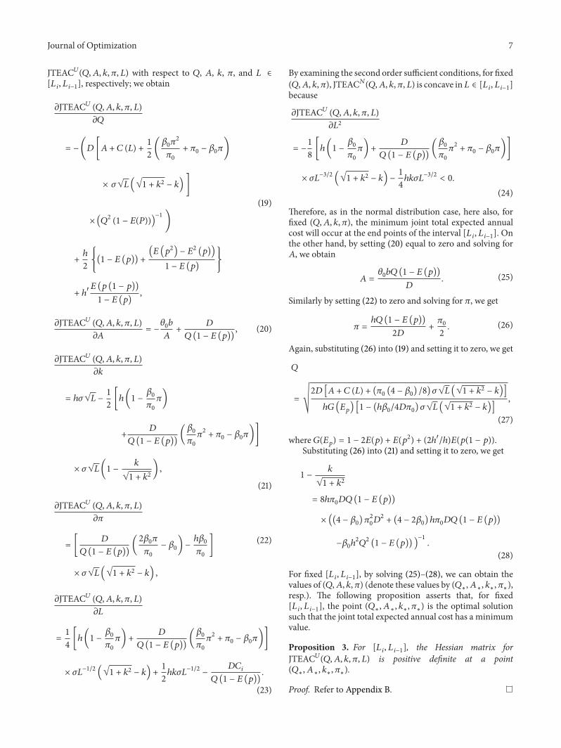
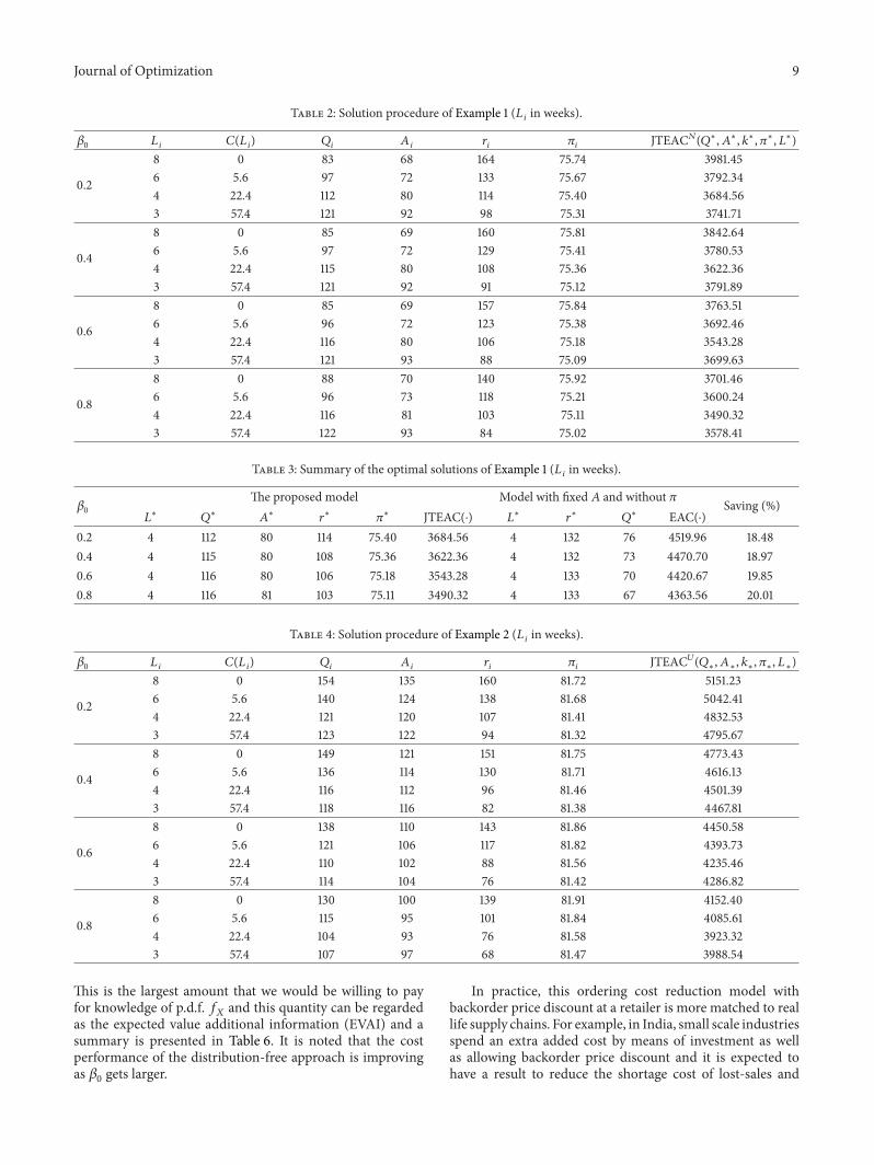
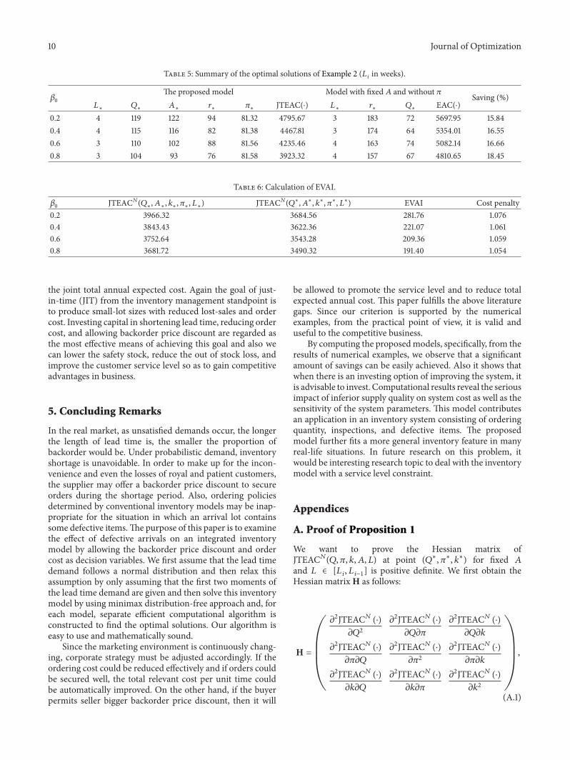
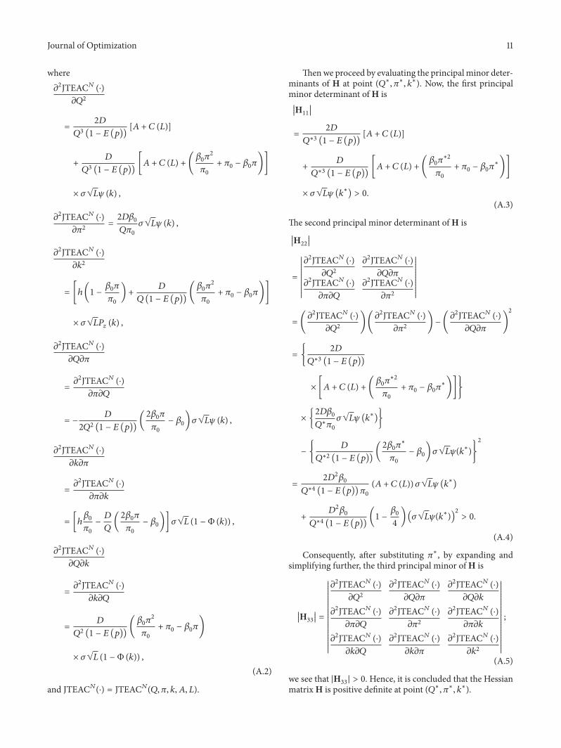
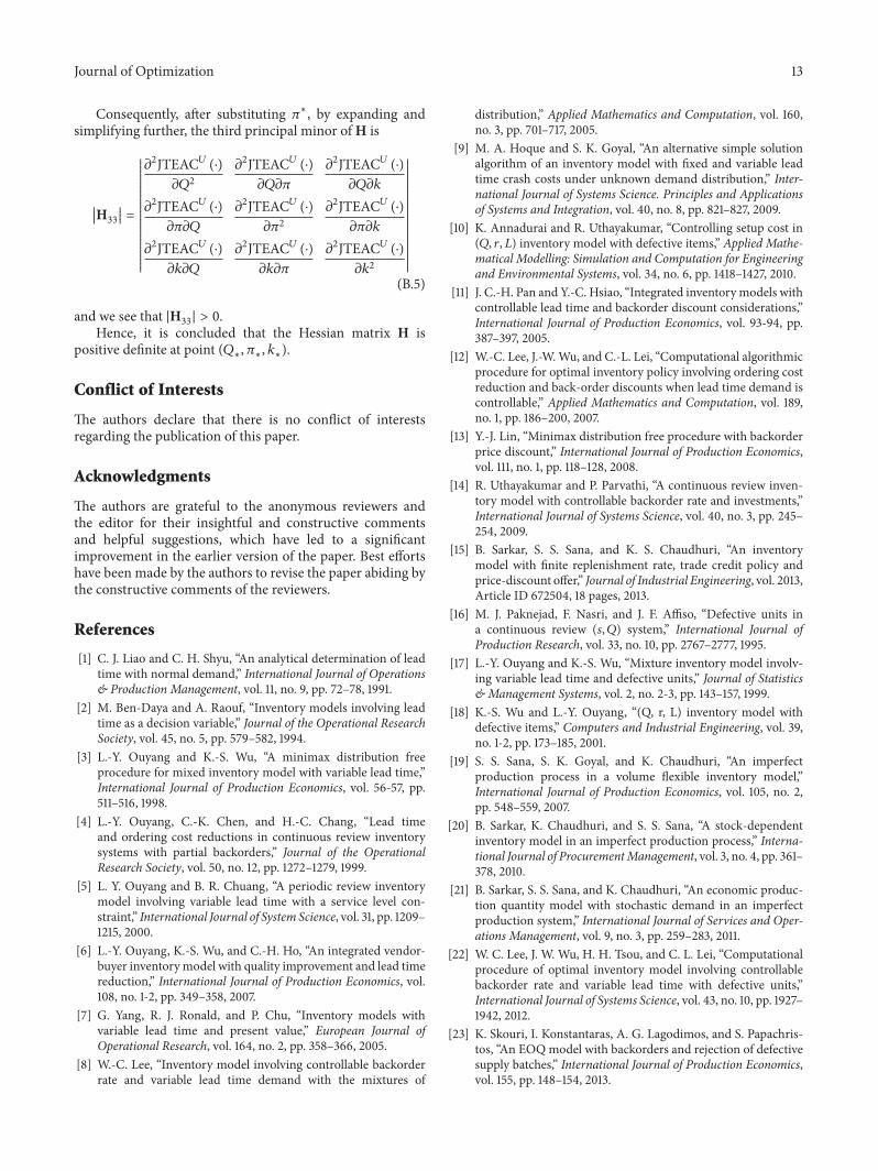