RESEARCH ARTICLE Open Access Predicting outcomes of steady

RESEARCH ARTICLE Open Access

Predicting outcomes of steady-state 13C isotopetracing experiments using Monte Carlo samplingJan Schellenberger1, Daniel C Zielinski2, Wing Choi2, Sunthosh Madireddi2, Vasiliy Portnoy2, David A Scott3,Jennifer L Reed4, Andrei L Osterman3 and Bernhard ∅ Palsson2*

Abstract

Background: Carbon-13 (13C) analysis is a commonly used method for estimating reaction rates in biochemicalnetworks. The choice of carbon labeling pattern is an important consideration when designing these experiments.We present a novel Monte Carlo algorithm for finding the optimal substrate input label for a particularexperimental objective (flux or flux ratio). Unlike previous work, this method does not require assumption of theflux distribution beforehand.

Results: Using a large E. coli isotopomer model, different commercially available substrate labeling patterns weretested computationally for their ability to determine reaction fluxes. The choice of optimal labeled substrate wasfound to be dependent upon the desired experimental objective. Many commercially available labels are predictedto be outperformed by complex labeling patterns. Based on Monte Carlo Sampling, the dimensionality ofexperimental data was found to be considerably less than anticipated, suggesting that effectiveness of 13Cexperiments for determining reaction fluxes across a large-scale metabolic network is less than previously believed.

Conclusions: While 13C analysis is a useful tool in systems biology, high redundancy in measurements limits theinformation that can be obtained from each experiment. It is however possible to compute potential limitationsbefore an experiment is run and predict whether, and to what degree, the rate of each reaction can be resolved.

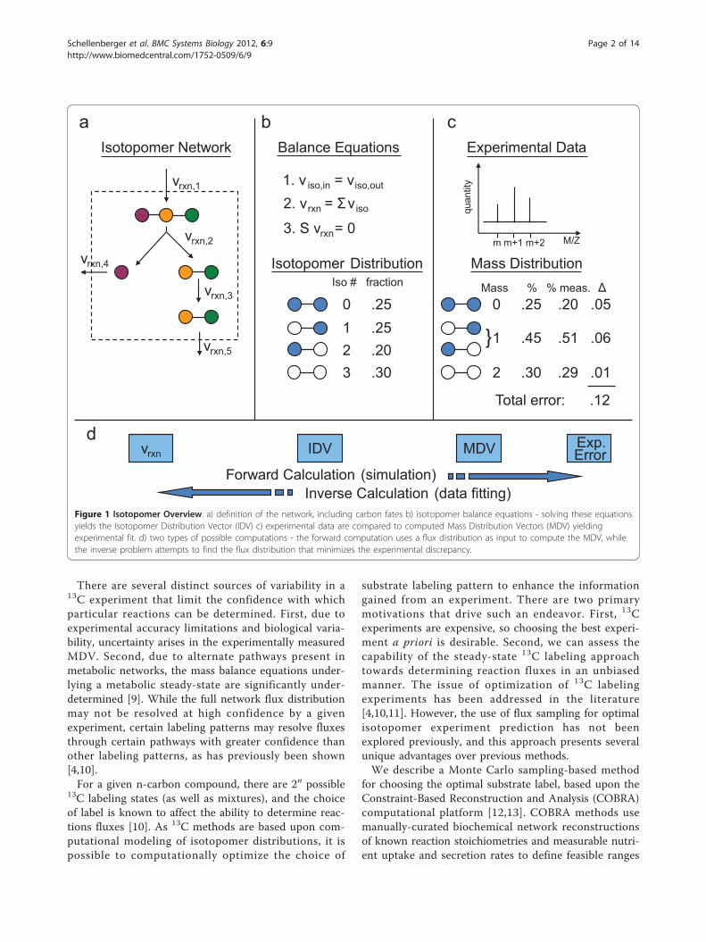
BackgroundIn vivo metabolic reaction flux data provides insight intothe dynamic function of the cell [1-3]. One widely-usedexperimental method for measuring in vivo reactionfluxes is steady-state substrate 13C isotope labeling [4-6].An overview of the general 13C methods is described inFigure 1. Isotopomers, or isomers created from insertinglabeled isotopes (often 13C) at different positions in amolecule, provide a unique way to track the progress ofcarbon through a metabolic network. By measuring theenrichment for 13C in metabolite pools after growing ona 13C labeled substrate, inferences about the internalflux state can be made. The approach can be summar-ized as a data fitting problem between simulated andexperimentally measured 13C labeled metabolite concen-trations. An isotopomer model, describing the positionaltransfer of carbon atoms for all or a subset of reactions

in the network, is used to simulate data (Figure 1a). Fora specified carbon input label, an isotopomer modelenables the calculation of an isotopomer distributionvector (IDV) corresponding to a particular simulatedsteady-state flux distribution (Figure 1b). Mass spectro-metry (MS) experiments on 13C-labeled metabolites (e.g.macromolecules) generate fractional 13C enrichmentsfrom fragmented macromolecules, forming a mass dis-tribution vector (MDV) (Figure 1c). The error betweenthe measured MDV and the MDV corresponding to thesimulated IDV summarizes how well the presumed fluxdistribution fits the 13C experiment. The flux distribu-tion v that minimizes this error can be computed by sol-ving a non-linear optimization problem. Simulating 13Cenrichment given a flux distribution is computationallyinexpensive; however, the inverse problem of calculatingthe flux distribution that best fits a 13C experiment isboth of greater interest and significantly more computa-tionally difficult (Figure 1d). A review of these methodsand associated challenges can be found in [6-8].

* Correspondence: [email protected] of Bioengineering, University of California - San Diego, 9500Gilman Drive, La Jolla, CA, 92093-0412 USAFull list of author information is available at the end of the article

Schellenberger et al. BMC Systems Biology 2012, 6:9http://www.biomedcentral.com/1752-0509/6/9

© 2012 Schellenberger et al. ; licensee BioMed Central Ltd. This is an open access article distributed under the terms of the CreativeCommons Attribution License (http://creativecommons.org/licenses/by/2.0), which permits unrestricted use, distribution, andreproduction in any medium, provided the original work is properly cited.

mailto:[email protected]

http://creativecommons.org/licenses/by/2.0

There are several distinct sources of variability in a13C experiment that limit the confidence with whichparticular reactions can be determined. First, due toexperimental accuracy limitations and biological varia-bility, uncertainty arises in the experimentally measuredMDV. Second, due to alternate pathways present inmetabolic networks, the mass balance equations under-lying a metabolic steady-state are significantly under-determined [9]. While the full network flux distributionmay not be resolved at high confidence by a givenexperiment, certain labeling patterns may resolve fluxesthrough certain pathways with greater confidence thanother labeling patterns, as has previously been shown[4,10].For a given n-carbon compound, there are 2n possible

13C labeling states (as well as mixtures), and the choiceof label is known to affect the ability to determine reac-tions fluxes [10]. As 13C methods are based upon com-putational modeling of isotopomer distributions, it ispossible to computationally optimize the choice of

substrate labeling pattern to enhance the informationgained from an experiment. There are two primarymotivations that drive such an endeavor. First, 13Cexperiments are expensive, so choosing the best experi-ment a priori is desirable. Second, we can assess thecapability of the steady-state 13C labeling approachtowards determining reaction fluxes in an unbiasedmanner. The issue of optimization of 13C labelingexperiments has been addressed in the literature[4,10,11]. However, the use of flux sampling for optimalisotopomer experiment prediction has not beenexplored previously, and this approach presents severalunique advantages over previous methods.We describe a Monte Carlo sampling-based method

for choosing the optimal substrate label, based upon theConstraint-Based Reconstruction and Analysis (COBRA)computational platform [12,13]. COBRA methods usemanually-curated biochemical network reconstructionsof known reaction stoichiometries and measurable nutri-ent uptake and secretion rates to define feasible ranges

Isotopomer Network Balance Equations

1. v iso,in = viso,out

2. vrxn = Σviso

3. S vrxn = 0

0 .25 1 .25 2 .20 3 .30

Isotopomer Distribution

Experimental Data

Mass Distribution

0 .25 .20 .05

1 .45 .51 .06

2 .30 .29 .01

M/Z m m+1 m+2

quan

tity

}

Mass % % meas. Δ Iso # fraction

vrxn,2

vrxn,3

vrxn,1

vrxn,4

vrxn,5

Total error: .12

vrxn IDV MDV Exp. Error

Forward Calculation (simulation) Inverse Calculation (data fitting)

a b c

d

Figure 1 Isotopomer Overview. a) definition of the network, including carbon fates b) isotopomer balance equations - solving these equationsyields the Isotopomer Distribution Vector (IDV) c) experimental data are compared to computed Mass Distribution Vectors (MDV) yieldingexperimental fit. d) two types of possible computations - the forward computation uses a flux distribution as input to compute the MDV, whilethe inverse problem attempts to find the flux distribution that minimizes the experimental discrepancy.


Page 2 of 14

for internal reaction fluxes. Many of these reconstruc-tions have been generated [14] and the procedure iswell-established [13,15]. These models can be used formethods such as computing growth rates [16,17], pre-dicting the effects of gene knockouts [16,18,19], predict-ing the endpoint of adaptive evolutions [20], anddesigning strains for industrial production [21,22]. Areview of these methods can be found here [12,13,23].Monte Carlo sampling of constraint-based metabolicmodels can be used to generate sets of biochemicallyfeasible flux distributions that obey measured uptakeand secretion rate constraints [24]. IDVs generated fromthese flux distributions in an isotopomer model canthen be compared against simulated 13C data to evaluatethe ability of the experiment to determine reactionfluxes. Monte Carlo sampling takes advantage of thespeed with which IDVs can be simulated from putativeflux distributions, making this approach suitable forlarge-scale analysis of in silico experiments.A Monte Carlo sampling approach was implemented

using a newly developed isotopomer model to evaluatethe efficiency of different carbon labeling patternstoward determining reaction fluxes in E. coli. Thedimensionality of simulated 13C data was calculatedusing singular value decomposition (SVD) for differentsubstrate labeling patterns and compared to the numberof undetermined dimensions in the network. 13C experi-ments were performed for three substrate labeling pat-terns to validate the prior theoretical analysis. Themethods developed represent a flexible computationalanalysis that can be applied to various biological systemsand experimental setups to estimate, a priori, the effi-ciency of isotopomer experiments in determining reac-tion fluxes.

Results and DiscussionExpanded Isotopomer ModelAn isotopomer model was constructed in two phases.First, a central metabolic isotopomer model thataccounts for 85 reactions including glycolysis, the TCAcycle, the pentose phosphate pathway, oxidative phos-phorylation, pyruvate metabolism, and anaplerotic reac-tions was derived from the iJR904 E. coli reconstruction[16]. This initial model was equivalent in reaction con-tent to commonly used isotopomer models for E. coli[25,26].An expanded model was then constructed that

includes both central and biosynthetic pathways. TheiMC1010 metabolic network [19] was evaluated todetermine which reactions can sustain non-zero fluxesduring growth on glucose, acetate, or lactate when onlycertain by-products are allowed to be secreted (acetate,formate, D-lactate, pyruvate, succinate, glycerol, CO2,and ethanol). Blocked reactions, which must have zero

net flux at steady state, were subsequently omitted fromconsideration. Groups of reactions that could be mergedtogether without affecting model results (e.g. linearpathways) were combined in order to reduce the num-ber of variables. Large sets of biosynthesis reactions thatproduce phospholipids, nucleotides, co-factors were alsocombined, since there no experimental measurementsexisted for these high-carbon metabolites. However, by-products resulting from high-carbon metabolite produc-tion (e.g. CO2, formate, succinate, fumarate, and pyru-vate) that could enter back into the metabolic networkwere tracked. Of the original 932 reactions in the com-plete metabolic iMC1010 network, nearly a third wererepresented in the biosynthetic isotopomer model, eitherindividually or as grouped reactions.The final isotopomer model accounts for a total of

313 irreversible reactions, including 278 which trackcarbon. Inclusion of these additional pathways is likelyimportant for accurate assessment of the flux-resolvingpower of 13C experiments both within and beyond cen-tral metabolism [7]. A complete listing of the reactionsand metabolites in the biosynthetic network can befound in the Additional File 1.

Monte Carlo Sampling ApproachTo compute possible flux distributions of the E. colimodel, the network was sampled using a Markov Chain,Monte Carlo (MCMC) sampling algorithm (see Meth-ods). The steady-state mass balance and uptake rateconstraints for the metabolic network create a convexhyperspace that contains all biochemically feasiblesteady-state flux distributions [27]. Monte Carlo sam-pling generates a set of flux distributions that are spreaduniformly throughout the feasible space. The inclusionof 13C experimental data reduces the feasible space inwhich the true flux state must lie by requiring that theIDV calculated from the putative flux distribution mustmatch the experimental data within error. While thespace of feasible flux distributions depends only on reac-tion stoichiometry, the space of resulting simulatedIDVs differs depending on the input substrate labelingpattern. Hence, different labeling patterns can have dif-fering abilities to resolve each reaction flux.Here, we used Monte Carlo sampling of flux distribu-

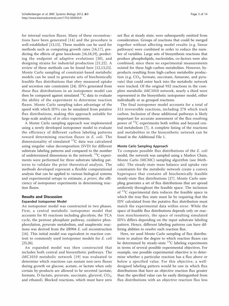
tions to analyze the degree to which reaction fluxes canbe determined by steady-state 13C labeling experimentsin terms of several possible experimental objectives. Forexample, one possible experimental objective is to deter-mine whether a particular reaction has a flux above orbelow a specified value. For this objective, a well-designed labeling pattern would be one in which fluxdistributions that have an objective reaction flux greaterthan the specified value can be easily distinguished fromflux distributions with an objective reaction flux less


Page 3 of 14

than the specified value. As seen in Figure 2, a hypothe-tical experiment 1 produces measurement distributionswhich overlap whereas experiment 2 shows greaterseparation. If one were interested in differentiatingbetween the two partitions, experiment 2 would bemuch preferable. This method allows for the scoring ofany label for any given experimental objective withoutfirst knowing the true cellular flux distribution v.

Generating and Evaluating 13C Experimental HypothesesAn experimental hypothesis is defined as a partition ofthe sampled flux distribution set. While many possiblehypotheses could be considered, two rational hypotheseswere studied. The first case attempts to elucidate

whether a reaction has high or low flux (hi-lo). Thesolution space is partitioned into all points with vj>threshold versus vj <threshold. A different hypothesisis generated for each reaction j. The threshold was cho-sen to be the median of all vj so that half of all pointswould be in each of the two partitions. The second setof hypotheses tested consisted of biologically relevantflux ratios. For each point the ratio of two reactions, vi/vj, was determined to be above or below some thresholdthat formed a partition.Intuitively, a hypothesis score should be high if the

isotopomer distributions coming from one partition aredistinguishable from distributions in the other partition.While there are several ways of doing this, we chose a

80% 20%

30% 20% 50%

C-12 C-13

}

}

Experiment 1

Experiment 2

Glucose Isotopomer Mixture Measurement Distribution

b

a

Partitio

n 1

Partitio

n 2

Fragments

Fragments

S v = 0

vlb < v < vub

Flux Constraints

Hi Lo Hypothesis

hypothesis score (e.g. flux vi)# sa

mpl

e po

ints

hypothesis score (e.g. flux vi)# sa

mpl

e po

ints

Figure 2 Method Overview. a) The space of flux distributions is partitioned in two parts corresponding to ‘high’ flux versus ‘low’ flux. A uniformrandom sample is drawn from the space and is also partitioned into partition 1 and partition 2. b) For each point in the space the distributionof experimental measurements is simulated. Hypothetical experiment 1 and experiment 2 with different glucose label mixtures produce differentmeasurement distributions. The distributions from experiment 2 are more separated, indicating parameters of experiment 2 are more conducivefor differentiating between the high and low partition.


Page 4 of 14

heuristic metric based on a Z-score, which is commonlyused to determine the difference between two samples.A Z-score was calculated for each fragment (element) ofthe calculated MDV for each simulated flux distribution:

Zi =|x̄hi − x̄lo|√s2hi + s2lo + σ 2

where x̄hi and x̄lo are the average fragment enrich-ments for the upper and lower partitions, respectively,s2hi and s2lo are the variances of fragment enrichments

for the upper and lower partitions, respectively, and thea is a constant equal to 0.014. a is on the order of mag-nitude of the uncertainty in measurements. This slightmodification to the standard Z-score puts a lowerbound on the expected experimental variation. The Z-score of each fragment is added together to give the Z-score of the experiment.

Z =∑

i∈fragment

Zi

Using this approach, candidate flux states weresampled uniformly and experimental hypotheses tested.Z-scores were calculated for the hi-lo hypothesis corre-sponding to 1) individual reactions 2) reaction ratiosand 3) two ‘random’ reactions or ratios. Randomhypotheses were tested to estimate the level of noise

associated with the set of flux distributions. Raw andnormalized Z-scores are given in the Additional File 1.Z-scores varied from the level of noise to a maximum of>20-fold the level of noise.To illustrate the differences in label-dependent reac-

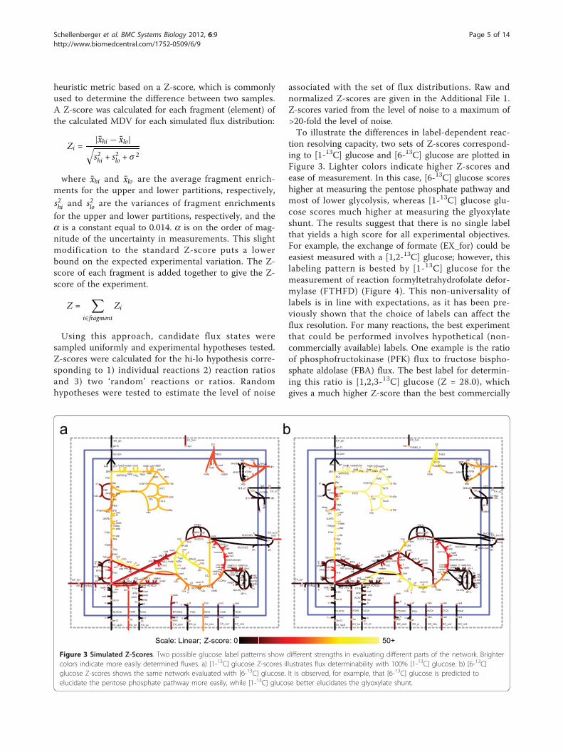
tion resolving capacity, two sets of Z-scores correspond-ing to [1-13C] glucose and [6-13C] glucose are plotted inFigure 3. Lighter colors indicate higher Z-scores andease of measurement. In this case, [6-13C] glucose scoreshigher at measuring the pentose phosphate pathway andmost of lower glycolysis, whereas [1-13C] glucose glu-cose scores much higher at measuring the glyoxylateshunt. The results suggest that there is no single labelthat yields a high score for all experimental objectives.For example, the exchange of formate (EX_for) could beeasiest measured with a [1,2-13C] glucose; however, thislabeling pattern is bested by [1-13C] glucose for themeasurement of reaction formyltetrahydrofolate defor-mylase (FTHFD) (Figure 4). This non-universality oflabels is in line with expectations, as it has been pre-viously shown that the choice of labels can affect theflux resolution. For many reactions, the best experimentthat could be performed involves hypothetical (non-commercially available) labels. One example is the ratioof phosphofructokinase (PFK) flux to fructose bispho-sphate aldolase (FBA) flux. The best label for determin-ing this ratio is [1,2,3-13C] glucose (Z = 28.0), whichgives a much higher Z-score than the best commercially

50+Z-score: 0Scale: Linear;

ba

Figure 3 Simulated Z-Scores. Two possible glucose label patterns show different strengths in evaluating different parts of the network. Brightercolors indicate more easily determined fluxes. a) [1-13C] glucose Z-scores illustrates flux determinability with 100% [1-13C] glucose. b) [6-13C]glucose Z-scores shows the same network evaluated with [6-13C] glucose. It is observed, for example, that [6-13C] glucose is predicted toelucidate the pentose phosphate pathway more easily, while [1-13C] glucose better elucidates the glyoxylate shunt.


Page 5 of 14

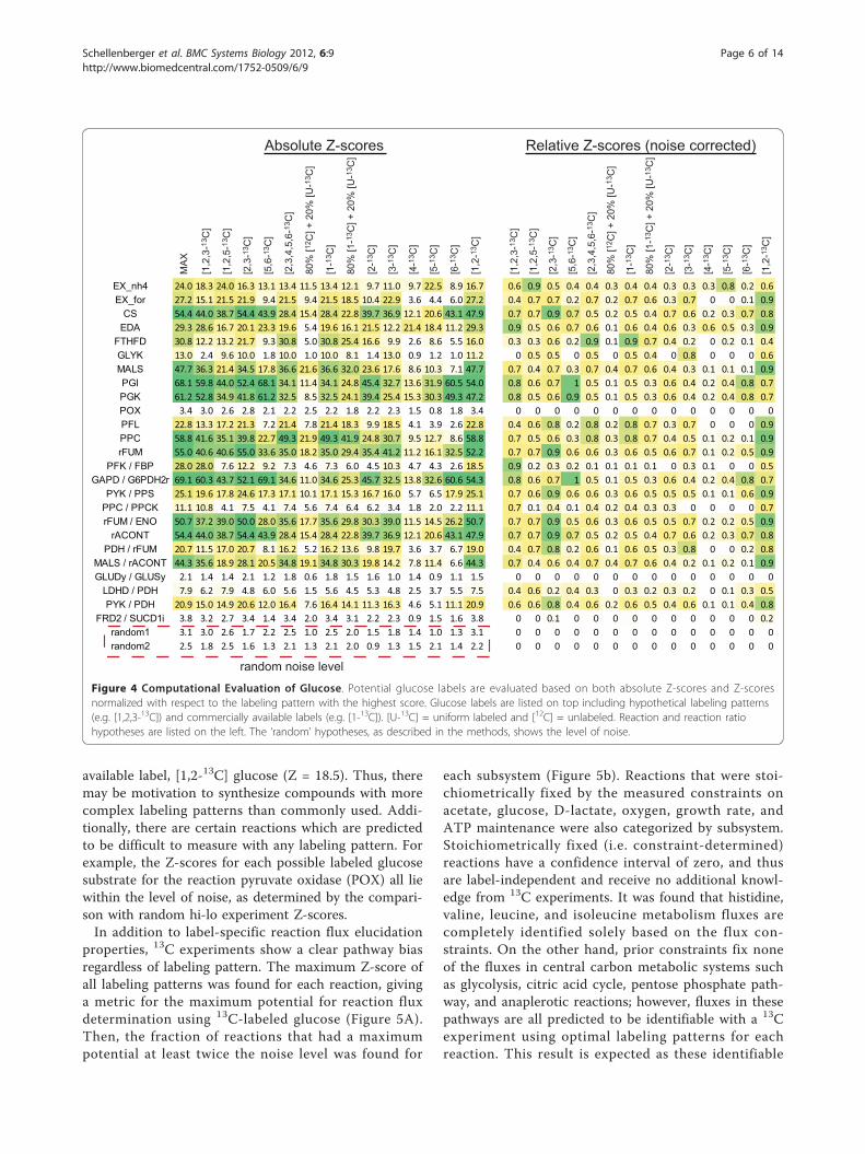
available label, [1,2-13C] glucose (Z = 18.5). Thus, theremay be motivation to synthesize compounds with morecomplex labeling patterns than commonly used. Addi-tionally, there are certain reactions which are predictedto be difficult to measure with any labeling pattern. Forexample, the Z-scores for each possible labeled glucosesubstrate for the reaction pyruvate oxidase (POX) all liewithin the level of noise, as determined by the compari-son with random hi-lo experiment Z-scores.In addition to label-specific reaction flux elucidation

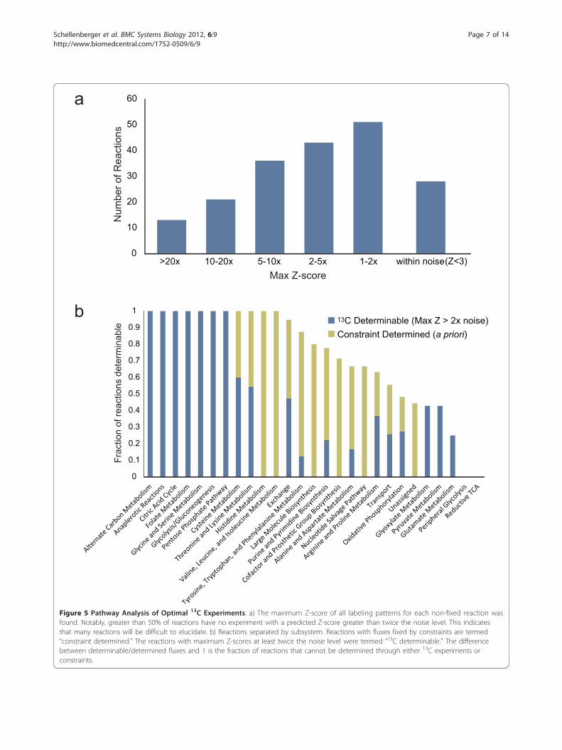
properties, 13C experiments show a clear pathway biasregardless of labeling pattern. The maximum Z-score ofall labeling patterns was found for each reaction, givinga metric for the maximum potential for reaction fluxdetermination using 13C-labeled glucose (Figure 5A).Then, the fraction of reactions that had a maximumpotential at least twice the noise level was found for

each subsystem (Figure 5b). Reactions that were stoi-chiometrically fixed by the measured constraints onacetate, glucose, D-lactate, oxygen, growth rate, andATP maintenance were also categorized by subsystem.Stoichiometrically fixed (i.e. constraint-determined)reactions have a confidence interval of zero, and thusare label-independent and receive no additional knowl-edge from 13C experiments. It was found that histidine,valine, leucine, and isoleucine metabolism fluxes arecompletely identified solely based on the flux con-straints. On the other hand, prior constraints fix noneof the fluxes in central carbon metabolic systems suchas glycolysis, citric acid cycle, pentose phosphate path-way, and anaplerotic reactions; however, fluxes in thesepathways are all predicted to be identifiable with a 13Cexperiment using optimal labeling patterns for eachreaction. This result is expected as these identifiable

EX_nh4 24.0 18.3 24.0 16.3 13.1 13.4 11.5 13.4 12.1 9.7 11.0 9.7 22.5 8.9 16.7 0.6 0.9 0.5 0.4 0.4 0.3 0.4 0.4 0.3 0.3 0.3 0.8 0.2 0.6EX_for 27.2 15.1 21.5 21.9 9.4 21.5 9.4 21.5 18.5 10.4 22.9 3.6 4.4 6.0 27.2 0.4 0.7 0.7 0.2 0.7 0.2 0.7 0.6 0.3 0.7 0 0 0.1 0.9

CS 54.4 44.0 38.7 54.4 43.9 28.4 15.4 28.4 22.8 39.7 36.9 12.1 20.6 43.1 47.9 0.7 0.7 0.9 0.7 0.5 0.2 0.5 0.4 0.7 0.6 0.2 0.3 0.7 0.8EDA 29.3 28.6 16.7 20.1 23.3 19.6 5.4 19.6 16.1 21.5 12.2 21.4 18.4 11.2 29.3 0.9 0.5 0.6 0.7 0.6 0.1 0.6 0.4 0.6 0.3 0.6 0.5 0.3 0.9

FTHFD 30.8 12.2 13.2 21.7 9.3 30.8 5.0 30.8 25.4 16.6 9.9 2.6 8.6 5.5 16.0 0.3 0.3 0.6 0.2 0.9 0.1 0.9 0.7 0.4 0.2 0 0.2 0.1 0.4GLYK 13.0 2.4 9.6 10.0 1.8 10.0 1.0 10.0 8.1 1.4 13.0 0.9 1.2 1.0 11.2 0 0.5 0.5 0 0.5 0 0.5 0.4 0 0.8 0 0 0 0.6MALS 47.7 36.3 21.4 34.5 17.8 36.6 21.6 36.6 32.0 23.6 17.6 8.6 10.3 7.1 47.7 0.7 0.4 0.7 0.3 0.7 0.4 0.7 0.6 0.4 0.3 0.1 0.1 0.1 0.9PGI 68.1 59.8 44.0 52.4 68.1 34.1 11.4 34.1 24.8 45.4 32.7 13.6 31.9 60.5 54.0 0.8 0.6 0.7 1 0.5 0.1 0.5 0.3 0.6 0.4 0.2 0.4 0.8 0.7PGK 61.2 52.8 34.9 41.8 61.2 32.5 8.5 32.5 24.1 39.4 25.4 15.3 30.3 49.3 47.2 0.8 0.5 0.6 0.9 0.5 0.1 0.5 0.3 0.6 0.4 0.2 0.4 0.8 0.7POX 3.4 3.0 2.6 2.8 2.1 2.2 2.5 2.2 1.8 2.2 2.3 1.5 0.8 1.8 3.4 0 0 0 0 0 0 0 0 0 0 0 0 0 0PFL 22.8 13.3 17.2 21.3 7.2 21.4 7.8 21.4 18.3 9.9 18.5 4.1 3.9 2.6 22.8 0.4 0.6 0.8 0.2 0.8 0.2 0.8 0.7 0.3 0.7 0 0 0 0.9PPC 58.8 41.6 35.1 39.8 22.7 49.3 21.9 49.3 41.9 24.8 30.7 9.5 12.7 8.6 58.8 0.7 0.5 0.6 0.3 0.8 0.3 0.8 0.7 0.4 0.5 0.1 0.2 0.1 0.9rFUM 55.0 40.6 40.6 55.0 33.6 35.0 18.2 35.0 29.4 35.4 41.2 11.2 16.1 32.5 52.2 0.7 0.7 0.9 0.6 0.6 0.3 0.6 0.5 0.6 0.7 0.1 0.2 0.5 0.9

PFK / FBP 28.0 28.0 7.6 12.2 9.2 7.3 4.6 7.3 6.0 4.5 10.3 4.7 4.3 2.6 18.5 0.9 0.2 0.3 0.2 0.1 0.1 0.1 0.1 0 0.3 0.1 0 0 0.5GAPD / G6PDH2r 69.1 60.3 43.7 52.1 69.1 34.6 11.0 34.6 25.3 45.7 32.5 13.8 32.6 60.6 54.3 0.8 0.6 0.7 1 0.5 0.1 0.5 0.3 0.6 0.4 0.2 0.4 0.8 0.7

PYK / PPS 25.1 19.6 17.8 24.6 17.3 17.1 10.1 17.1 15.3 16.7 16.0 5.7 6.5 17.9 25.1 0.7 0.6 0.9 0.6 0.6 0.3 0.6 0.5 0.5 0.5 0.1 0.1 0.6 0.9PPC / PPCK 11.1 10.8 4.1 7.5 4.1 7.4 5.6 7.4 6.4 6.2 3.4 1.8 2.0 2.2 11.1 0.7 0.1 0.4 0.1 0.4 0.2 0.4 0.3 0.3 0 0 0 0 0.7rFUM / ENO 50.7 37.2 39.0 50.0 28.0 35.6 17.7 35.6 29.8 30.3 39.0 11.5 14.5 26.2 50.7 0.7 0.7 0.9 0.5 0.6 0.3 0.6 0.5 0.5 0.7 0.2 0.2 0.5 0.9

rACONT 54.4 44.0 38.7 54.4 43.9 28.4 15.4 28.4 22.8 39.7 36.9 12.1 20.6 43.1 47.9 0.7 0.7 0.9 0.7 0.5 0.2 0.5 0.4 0.7 0.6 0.2 0.3 0.7 0.8PDH / rFUM 20.7 11.5 17.0 20.7 8.1 16.2 5.2 16.2 13.6 9.8 19.7 3.6 3.7 6.7 19.0 0.4 0.7 0.8 0.2 0.6 0.1 0.6 0.5 0.3 0.8 0 0 0.2 0.8

MALS / rACONT 44.3 35.6 18.9 28.1 20.5 34.8 19.1 34.8 30.3 19.8 14.2 7.8 11.4 6.6 44.3 0.7 0.4 0.6 0.4 0.7 0.4 0.7 0.6 0.4 0.2 0.1 0.2 0.1 0.9GLUDy / GLUSy 2.1 1.4 1.4 2.1 1.2 1.8 0.6 1.8 1.5 1.6 1.0 1.4 0.9 1.1 1.5 0 0 0 0 0 0 0 0 0 0 0 0 0 0

LDHD / PDH 7.9 6.2 7.9 4.8 6.0 5.6 1.5 5.6 4.5 5.3 4.8 2.5 3.7 5.5 7.5 0.4 0.6 0.2 0.4 0.3 0 0.3 0.2 0.3 0.2 0 0.1 0.3 0.5PYK / PDH 20.9 15.0 14.9 20.6 12.0 16.4 7.6 16.4 14.1 11.3 16.3 4.6 5.1 11.1 20.9 0.6 0.6 0.8 0.4 0.6 0.2 0.6 0.5 0.4 0.6 0.1 0.1 0.4 0.8

FRD2 / SUCD1i 3.8 3.2 2.7 3.4 1.4 3.4 2.0 3.4 3.1 2.2 2.3 0.9 1.5 1.6 3.8 0 0 0.1 0 0 0 0 0 0 0 0 0 0 0.2random1 3.1 3.0 2.6 1.7 2.2 2.5 1.0 2.5 2.0 1.5 1.8 1.4 1.0 1.3 3.1 0 0 0 0 0 0 0 0 0 0 0 0 0 0random2 2.5 1.8 2.5 1.6 1.3 2.1 1.3 2.1 2.0 0.9 1.3 1.5 2.1 1.4 2.2 0 0 0 0 0 0 0 0 0 0 0 0 0 0

Absolute Z-scores Relative Z-scores (noise corrected)

[1,2

-13 C

]

[6-1

3 C]

[5-1

3 C]

[4-1

3 C]

[3-1

3 C]

[2-1

3 C]

80%

[1-1

3 C] +

20%

[U-1

3 C]

[1-1

3 C]

80%

[12 C

] + 2

0% [U

-13 C

]

[2,3

,4,5

,6-1

3 C]

[5,6

-13 C

]

[2,3

-13 C

]

[1,2

,5-1

3 C]

[1,2

,3-1

3 C]

MA

X

[1,2

-13 C

]

[6-1

3 C]

[5-1

3 C]

[4-1

3 C]

[3-1

3 C]

[2-1

3 C]

80%

[1-1

3 C] +

20%

[U-1

3 C]

[1-1

3 C]

80%

[12 C

] + 2

0% [U

-13 C

]

[2,3

,4,5

,6-1

3 C]

[5,6

-13 C

]

[2,3

-13 C

]

[1,2

,5-1

3 C]

[1,2

,3-1

3 C]

random noise level

Figure 4 Computational Evaluation of Glucose. Potential glucose labels are evaluated based on both absolute Z-scores and Z-scoresnormalized with respect to the labeling pattern with the highest score. Glucose labels are listed on top including hypothetical labeling patterns(e.g. [1,2,3-13C]) and commercially available labels (e.g. [1-13C]). [U-13C] = uniform labeled and [12C] = unlabeled. Reaction and reaction ratiohypotheses are listed on the left. The ‘random’ hypotheses, as described in the methods, shows the level of noise.


Page 6 of 14

0

0.1

0.2

0.3

0.4

0.5

0.6

0.7

0.8

0.9

1

Constraint Determined (a priori)

13C Determinable (Max Z > 2x noise)

Frac

tion

of re

actio

ns d

eter

min

able

a

b

Num

ber o

f Rea

ctio

ns

0

10

20

30

40

50

60

>20x 10-20x 5-10x 2-5x 1-2x within noise(Z<3)Max Z-score

Figure 5 Pathway Analysis of Optimal 13C Experiments. a) The maximum Z-score of all labeling patterns for each non-fixed reaction wasfound. Notably, greater than 50% of reactions have no experiment with a predicted Z-score greater than twice the noise level. This indicatesthat many reactions will be difficult to elucidate. b) Reactions separated by subsystem. Reactions with fluxes fixed by constraints are termed“constraint determined.” The reactions with maximum Z-scores at least twice the noise level were termed “13C determinable.” The differencebetween determinable/determined fluxes and 1 is the fraction of reactions that cannot be determined through either 13C experiments orconstraints.


Page 7 of 14

pathways are the typical pathways being studied using13C analysis. Other pathways, such as cysteine, threo-nine, and lysine metabolism, are completely identifiablethrough a combination of prior stoichiometric con-straints combined with well-chosen 13C experiments.However, many of the remaining subsystems have afraction of reactions that cannot be determined usingany 13C-labeling pattern of glucose. In particular, noadditional information can be obtained from 13C-labeledglucose experiments about certain biosynthetic path-ways, nucleotide salvage pathways, reductive citric acidcycle reactions, and certain alternate pathways periph-eral to glycolysis, such as an alternate pathways fromDHAP to D-lactate. Measuring metabolites other thanamino acids may give more information on these path-ways. Note that in this discussion of identifiability, theZ-score metric indicates that an experiment can signifi-cantly reduce the confidence interval of a particularreaction but does not specifically predict the value ofthe confidence interval. Confidence intervals are directlycalculated for experimental data sets in a later sectionand compared to the Z-scores for the same labelingpatterns.

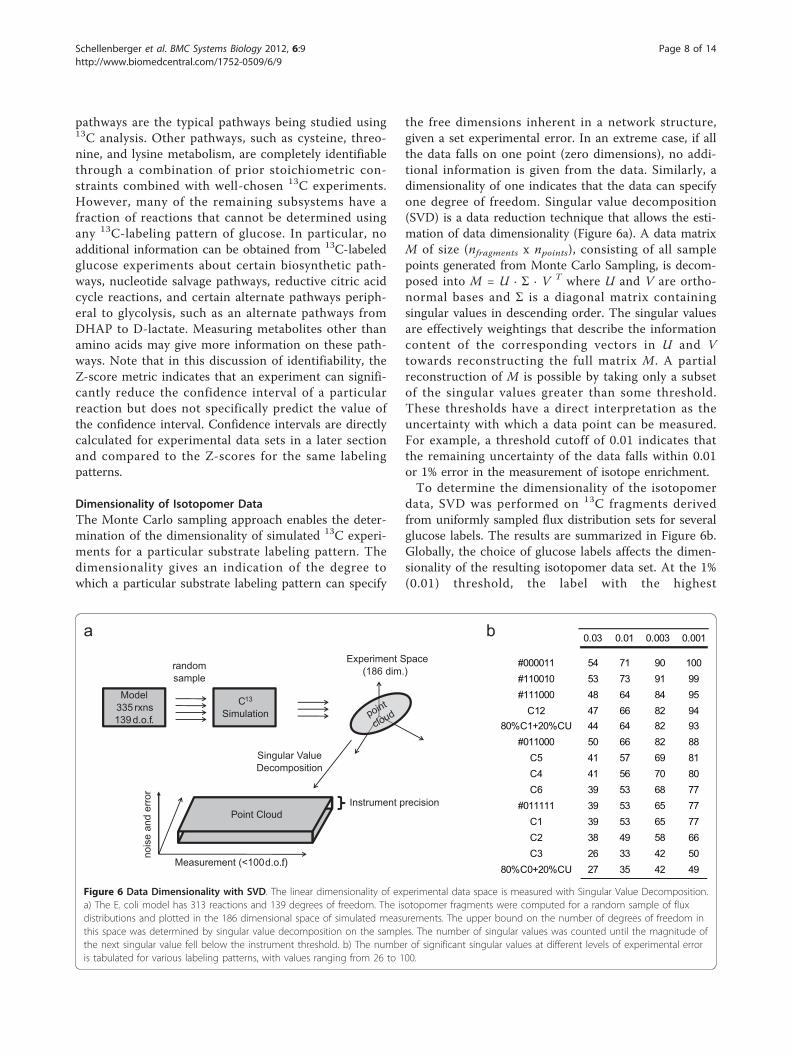
Dimensionality of Isotopomer DataThe Monte Carlo sampling approach enables the deter-mination of the dimensionality of simulated 13C experi-ments for a particular substrate labeling pattern. Thedimensionality gives an indication of the degree towhich a particular substrate labeling pattern can specify

the free dimensions inherent in a network structure,given a set experimental error. In an extreme case, if allthe data falls on one point (zero dimensions), no addi-tional information is given from the data. Similarly, adimensionality of one indicates that the data can specifyone degree of freedom. Singular value decomposition(SVD) is a data reduction technique that allows the esti-mation of data dimensionality (Figure 6a). A data matrixM of size (nfragments x npoints), consisting of all samplepoints generated from Monte Carlo Sampling, is decom-posed into M = U · Σ · V T where U and V are ortho-normal bases and Σ is a diagonal matrix containingsingular values in descending order. The singular valuesare effectively weightings that describe the informationcontent of the corresponding vectors in U and Vtowards reconstructing the full matrix M. A partialreconstruction of M is possible by taking only a subsetof the singular values greater than some threshold.These thresholds have a direct interpretation as theuncertainty with which a data point can be measured.For example, a threshold cutoff of 0.01 indicates thatthe remaining uncertainty of the data falls within 0.01or 1% error in the measurement of isotope enrichment.To determine the dimensionality of the isotopomer

data, SVD was performed on 13C fragments derivedfrom uniformly sampled flux distribution sets for severalglucose labels. The results are summarized in Figure 6b.Globally, the choice of glucose labels affects the dimen-sionality of the resulting isotopomer data set. At the 1%(0.01) threshold, the label with the highest

C13

Simulation

Experiment Space (186 dim.)

Measurement (<100 d.o.f.)

Point Cloud

nois

e an

d er

ror

Instrument precision

Model 335 rxns 139 d.o.f.

random sample

Singular Value Decomposition

0.03 0.01 0.003 0.001

#000011 54 71 90 100#110010 53 73 91 99#111000 48 64 84 95

C12 47 66 82 9480%C1+20%CU 44 64 82 93

#011000 50 66 82 88C5 41 57 69 81C4 41 56 70 80C6 39 53 68 77

#011111 39 53 65 77C1 39 53 65 77C2 38 49 58 66C3 26 33 42 50

80%C0+20%CU 27 35 42 49

a b

point

cloud

Figure 6 Data Dimensionality with SVD. The linear dimensionality of experimental data space is measured with Singular Value Decomposition.a) The E. coli model has 313 reactions and 139 degrees of freedom. The isotopomer fragments were computed for a random sample of fluxdistributions and plotted in the 186 dimensional space of simulated measurements. The upper bound on the number of degrees of freedom inthis space was determined by singular value decomposition on the samples. The number of singular values was counted until the magnitude ofthe next singular value fell below the instrument threshold. b) The number of significant singular values at different levels of experimental erroris tabulated for various labeling patterns, with values ranging from 26 to 100.


Page 8 of 14

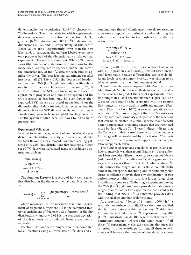
dimensionality was hypothetical [1,2,5-13C] glucose with73 dimensions. The three labels for which experimentaldata was measured in the subsequent section, [1-13C]glucose, [6-13C] glucose, and 20% [U-13C] glucose, haddimensions 53, 53 and 35, respectively, at this cutoff.These values are all significantly lower than the bestlabel, and, in particular, the uniform labeled experimentonly produces half of the dimensionality as the optimalexperiment. This result is significant. While 139 dimen-sions (the number of undetermined dimensions for themodel used) are required to specify a unique flux vector,the dimensionality of the 13C data for each label is sig-nificantly lower. The best labeling experiment specifiesjust over half (73/139 = 0.52) the degrees of freedomrequired, and 20% [U-13C] glucose only specifies aboutone fourth of the possible degrees of freedom (0.26). Itis worth noting that SVD is a linear operation used toapproximate properties of a non-linear system and thetrue degrees of freedom may be even lower thanreported. SVD serves as a useful upper bound on thedimensionality of data for non-linear systems, but thedifference between SVD dimensionality and true dimen-sionality may grow to be unacceptable for large systems.For the system studied here, SVD was found to be ofpractical use.

Experimental ValidationIn order to assess the agreement of computationally pre-dicted flux elucidation capacity with experimental data,we took fluxomic measurements for three labeling pat-terns in E. coli. Flux distributions that best explain eachset of 13C data were calculated using a non-linear opti-mization problem:

minv

Error(v)

subject to :vmin < v < vmax

S · v = 0

The function Error(v) is a score of how well a givenflux distribution fits the experimental data. It is definedas:

Error(v) =∑

i∈ fragments

(fragmenti(v) − measuredi)2

σ 2

where measured i is the measured fractional enrich-ment of fragment i, fragment i(v) is the computed frac-tional enrichment of fragment i as a function of the fluxdistribution v, and a = 0:014 is the standard deviationof the fragments as calculated from experimentalreplicates.Reaction flux confidence ranges were then computed

for all reactions using all three sets of 13C data and all

combinations thereof. Confidence intervals for reactionrates were computed by maximizing and minimizing thevalue of each reaction in turn subject to a slightlyrelaxed score.

minα

/maxα

cTi · N · αsubject to :

vmin ≤ N · α ≤ vmax

Error (N · α) ≤ Errormax

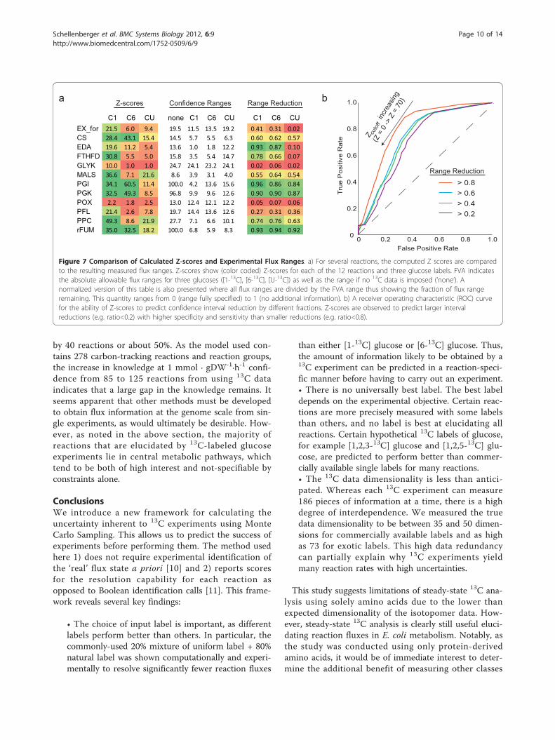
where ci = (0, 0, ...0, 1, 0...0) is a vector of all zeroswith a 1 in position i, and Errormax was set based on theconfidence value. Because different data sets provide dif-ferent levels of consistency, Errormax was chosen to be30 units greater than the minimum error found.These intervals were compared with Z-scores calcu-

lated through Monte Carlo methods to assess the abilityof the Z-scores to predict the size of experimental reac-tion ranges in a label-specific manner (Figure 7a). TheZ-scores were found to be correlated with the relativeflux ranges in a statistically significant manner (Stu-dent’s T-test, p <8.6 × 10-34). A receiver operating char-acteristic (ROC) curve suggests that the Z-scores canidentify with both sensitivity and specificity the reactionsthat can be elucidated in a label-specific manner, withbetter performance predicting ranges that are restrictedmore by data (Figure 7b). These findings indicate thatthe Z-score is indeed a useful predictor of the degree aflux range will be constrained by a particular 13C experi-ment and provide experimental support for the compu-tational approach taken.The number of reactions elucidated at particular con-

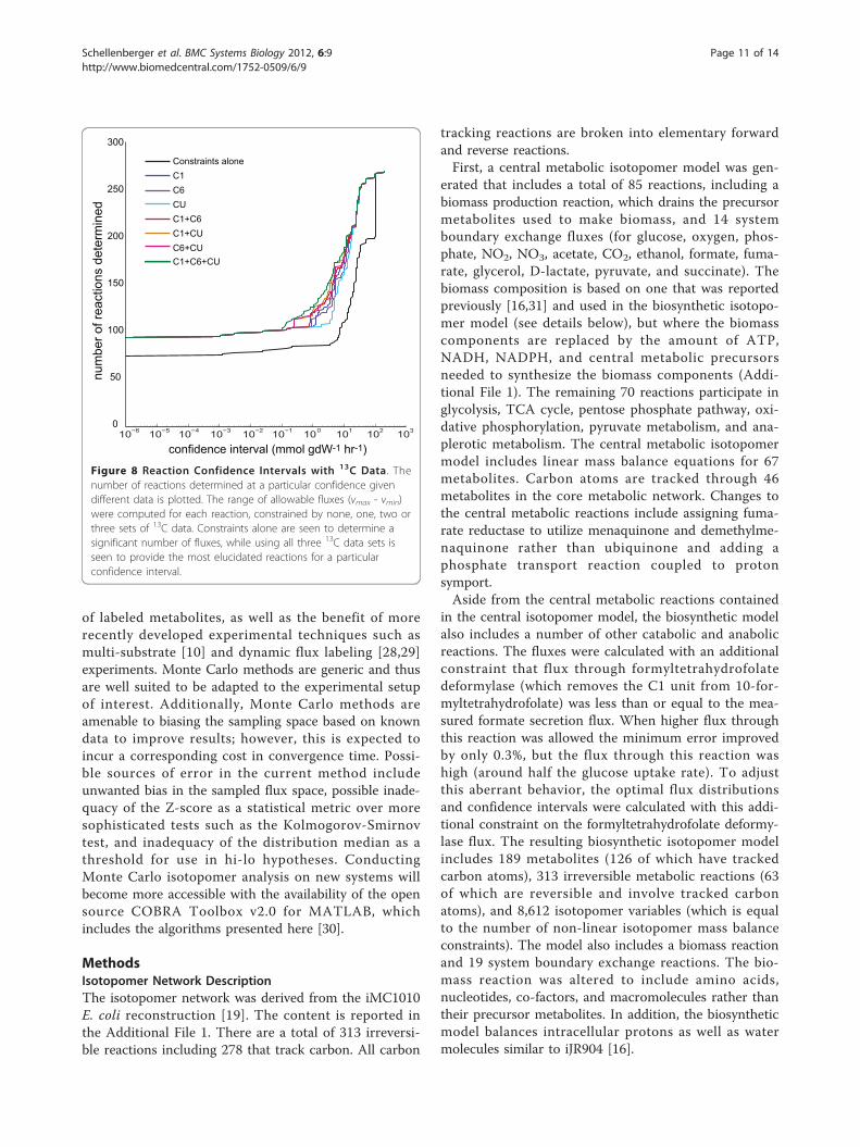
fidence intervals was then found (Figure 8). Using differ-ent labels provides different levels of reaction confidence(Additional File 1). Including no 13C data generates thelargest flux ranges (lower black line), while adding 13Cdata reduces the ranges and shifts the curve left. Withalmost no exception, including one experiment yieldslarger confidence intervals than any combination of twocarbon sources which in turn is a larger range thanincluding all three sets. Of the single experiment curves,the 20% [U-13C] glucose curve provides notably worseranges than the other two experiments, consistent withthe finding that 20% [U-13C] substrate provides datawith the smallest number of dimensions.At a reaction confidence of 1 mmol · gDW-1·h-1 (a

relatively non-stringent cutoff), 85 reactions are specifiedsimply from uptake rate data without any 13C data. Per-forming the least informative 13C experiment, using 20%[U-13C] substrate, yields 105 reactions that meet theconfidence criterion, whereas the combination of allthree 13C experiments yields 125 reactions that meet thecriterion. In other words, performing all three experi-ments will increase the number of elucidated reactions


Page 9 of 14

by 40 reactions or about 50%. As the model used con-tains 278 carbon-tracking reactions and reaction groups,the increase in knowledge at 1 mmol · gDW-1·h-1 confi-dence from 85 to 125 reactions from using 13C dataindicates that a large gap in the knowledge remains. Itseems apparent that other methods must be developedto obtain flux information at the genome scale from sin-gle experiments, as would ultimately be desirable. How-ever, as noted in the above section, the majority ofreactions that are elucidated by 13C-labeled glucoseexperiments lie in central metabolic pathways, whichtend to be both of high interest and not-specifiable byconstraints alone.

ConclusionsWe introduce a new framework for calculating theuncertainty inherent to 13C experiments using MonteCarlo Sampling. This allows us to predict the success ofexperiments before performing them. The method usedhere 1) does not require experimental identification ofthe ‘real’ flux state a priori [10] and 2) reports scoresfor the resolution capability for each reaction asopposed to Boolean identification calls [11]. This frame-work reveals several key findings:

• The choice of input label is important, as differentlabels perform better than others. In particular, thecommonly-used 20% mixture of uniform label + 80%natural label was shown computationally and experi-mentally to resolve significantly fewer reaction fluxes

than either [1-13C] glucose or [6-13C] glucose. Thus,the amount of information likely to be obtained by a13C experiment can be predicted in a reaction-speci-fic manner before having to carry out an experiment.• There is no universally best label. The best labeldepends on the experimental objective. Certain reac-tions are more precisely measured with some labelsthan others, and no label is best at elucidating allreactions. Certain hypothetical 13C labels of glucose,for example [1,2,3-13C] glucose and [1,2,5-13C] glu-cose, are predicted to perform better than commer-cially available single labels for many reactions.• The 13C data dimensionality is less than antici-pated. Whereas each 13C experiment can measure186 pieces of information at a time, there is a highdegree of interdependence. We measured the truedata dimensionality to be between 35 and 50 dimen-sions for commercially available labels and as highas 73 for exotic labels. This high data redundancycan partially explain why 13C experiments yieldmany reaction rates with high uncertainties.

This study suggests limitations of steady-state 13C ana-lysis using solely amino acids due to the lower thanexpected dimensionality of the isotopomer data. How-ever, steady-state 13C analysis is clearly still useful eluci-dating reaction fluxes in E. coli metabolism. Notably, asthe study was conducted using only protein-derivedamino acids, it would be of immediate interest to deter-mine the additional benefit of measuring other classes

C1 C6 CU none C1 C6 CU C1 C6 CUEX_for 21.5 6.0 9.4 19.5 11.5 13.5 19.2 0.41 0.31 0.02CS 28.4 43.1 15.4 14.5 5.7 5.5 6.3 0.60 0.62 0.57EDA 19.6 11.2 5.4 13.6 1.0 1.8 12.2 0.93 0.87 0.10FTHFD 30.8 5.5 5.0 15.8 3.5 5.4 14.7 0.78 0.66 0.07GLYK 10.0 1.0 1.0 24.7 24.1 23.2 24.1 0.02 0.06 0.02MALS 36.6 7.1 21.6 8.6 3.9 3.1 4.0 0.55 0.64 0.54PGI 34.1 60.5 11.4 100.0 4.2 13.6 15.6 0.96 0.86 0.84PGK 32.5 49.3 8.5 96.8 9.9 9.6 12.6 0.90 0.90 0.87POX 2.2 1.8 2.5 13.0 12.4 12.1 12.2 0.05 0.07 0.06PFL 21.4 2.6 7.8 19.7 14.4 13.6 12.6 0.27 0.31 0.36PPC 49.3 8.6 21.9 27.7 7.1 6.6 10.1 0.74 0.76 0.63rFUM 35.0 32.5 18.2 100.0 6.8 5.9 8.3 0.93 0.94 0.92

0 0.2

> 0.8> 0.6> 0.4> 0.2

0.60.4 0.8 1.0False Positive Rate

True

Pos

itive

Rat

e Z cuto

ff in

crea

sing

(Z =

0 ->

Z =

70)a b 1.0Z-scores Confidence Ranges Range Reduction

0.8

0.6

0.4

0.2

0

Range Reduction

Figure 7 Comparison of Calculated Z-scores and Experimental Flux Ranges. a) For several reactions, the computed Z scores are comparedto the resulting measured flux ranges. Z-scores show (color coded) Z-scores for each of the 12 reactions and three glucose labels. FVA indicatesthe absolute allowable flux ranges for three glucoses ([1-13C], [6-13C], [U-13C]) as well as the range if no 13C data is imposed (’none’). Anormalized version of this table is also presented where all flux ranges are divided by the FVA range thus showing the fraction of flux rangeremaining. This quantity ranges from 0 (range fully specified) to 1 (no additional information). b) A receiver operating characteristic (ROC) curvefor the ability of Z-scores to predict confidence interval reduction by different fractions. Z-scores are observed to predict larger intervalreductions (e.g. ratio<0.2) with higher specificity and sensitivity than smaller reductions (e.g. ratio<0.8).


Page 10 of 14

of labeled metabolites, as well as the benefit of morerecently developed experimental techniques such asmulti-substrate [10] and dynamic flux labeling [28,29]experiments. Monte Carlo methods are generic and thusare well suited to be adapted to the experimental setupof interest. Additionally, Monte Carlo methods areamenable to biasing the sampling space based on knowndata to improve results; however, this is expected toincur a corresponding cost in convergence time. Possi-ble sources of error in the current method includeunwanted bias in the sampled flux space, possible inade-quacy of the Z-score as a statistical metric over moresophisticated tests such as the Kolmogorov-Smirnovtest, and inadequacy of the distribution median as athreshold for use in hi-lo hypotheses. ConductingMonte Carlo isotopomer analysis on new systems willbecome more accessible with the availability of the opensource COBRA Toolbox v2.0 for MATLAB, whichincludes the algorithms presented here [30].

MethodsIsotopomer Network DescriptionThe isotopomer network was derived from the iMC1010E. coli reconstruction [19]. The content is reported inthe Additional File 1. There are a total of 313 irreversi-ble reactions including 278 that track carbon. All carbon

tracking reactions are broken into elementary forwardand reverse reactions.First, a central metabolic isotopomer model was gen-

erated that includes a total of 85 reactions, including abiomass production reaction, which drains the precursormetabolites used to make biomass, and 14 systemboundary exchange fluxes (for glucose, oxygen, phos-phate, NO2, NO3, acetate, CO2, ethanol, formate, fuma-rate, glycerol, D-lactate, pyruvate, and succinate). Thebiomass composition is based on one that was reportedpreviously [16,31] and used in the biosynthetic isotopo-mer model (see details below), but where the biomasscomponents are replaced by the amount of ATP,NADH, NADPH, and central metabolic precursorsneeded to synthesize the biomass components (Addi-tional File 1). The remaining 70 reactions participate inglycolysis, TCA cycle, pentose phosphate pathway, oxi-dative phosphorylation, pyruvate metabolism, and ana-plerotic metabolism. The central metabolic isotopomermodel includes linear mass balance equations for 67metabolites. Carbon atoms are tracked through 46metabolites in the core metabolic network. Changes tothe central metabolic reactions include assigning fuma-rate reductase to utilize menaquinone and demethylme-naquinone rather than ubiquinone and adding aphosphate transport reaction coupled to protonsymport.Aside from the central metabolic reactions contained

in the central isotopomer model, the biosynthetic modelalso includes a number of other catabolic and anabolicreactions. The fluxes were calculated with an additionalconstraint that flux through formyltetrahydrofolatedeformylase (which removes the C1 unit from 10-for-myltetrahydrofolate) was less than or equal to the mea-sured formate secretion flux. When higher flux throughthis reaction was allowed the minimum error improvedby only 0.3%, but the flux through this reaction washigh (around half the glucose uptake rate). To adjustthis aberrant behavior, the optimal flux distributionsand confidence intervals were calculated with this addi-tional constraint on the formyltetrahydrofolate deformy-lase flux. The resulting biosynthetic isotopomer modelincludes 189 metabolites (126 of which have trackedcarbon atoms), 313 irreversible metabolic reactions (63of which are reversible and involve tracked carbonatoms), and 8,612 isotopomer variables (which is equalto the number of non-linear isotopomer mass balanceconstraints). The model also includes a biomass reactionand 19 system boundary exchange reactions. The bio-mass reaction was altered to include amino acids,nucleotides, co-factors, and macromolecules rather thantheir precursor metabolites. In addition, the biosyntheticmodel balances intracellular protons as well as watermolecules similar to iJR904 [16].

10−6 10−5 10−4 10−3 10−2 10−1 100 101 102 103

confidence interval (mmol gdW-1 hr-1)

300

250

200

150

100

50

0

Constraints aloneC1C6CUC1+C6C1+CUC6+CUC1+C6+CU

num

ber o

f rea

ctio

ns d

eter

min

ed

Figure 8 Reaction Confidence Intervals with 13C Data. Thenumber of reactions determined at a particular confidence givendifferent data is plotted. The range of allowable fluxes (vmax - vmin)were computed for each reaction, constrained by none, one, two orthree sets of 13C data. Constraints alone are seen to determine asignificant number of fluxes, while using all three 13C data sets isseen to provide the most elucidated reactions for a particularconfidence interval.


Page 11 of 14

Monte Carlo SamplingWith traditional MCMC, a point is selected within thespace which is then iteratively moved around. At eachstep, a random direction is chosen and the next point ischosen uniformly along this line. The set of points thatthis algorithm visits will converge to a uniformly distrib-uted set. Two modifications were made: 1) ArtificialCentering [32] - Because these biological spaces tend tobe elongated in one direction, it is often beneficial tochoose directions along the “long” direction rather thanuniformly. This can be done by choosing the directionbased on previously visited points. At each step, thedirection is chosen by drawing a vector from the centerof the previous points to one of the previous points cho-sen at random. 2) In place sampling - Instead of movingjust one point throughout the space, many points aremoved simultaneously. In this way, no “history” is kept,only the updated position of all the points. This methodis described in greater detail in other literature [33,34].

Computing the Isotopomer DistributionEach flux distribution and glucose input results in aunique isotopomer distribution. The cumomer method[35] and the elementary metabolite unit (EMU) method[36] were implemented in Matlab and utilized in calcu-lating isotopomer distributions. These methods involvesolving several linear systems of equations to computedifferent groups of isotopomers. For numerical reasons,a routine is introduced which checks whether all partsof the network are still connected at every step. Discon-nected components can occur when fluxes to and fromthe component are zero, making it impossible to com-pute a unique isotopomer distribution within this sub-network as many isotopomers satisfy the balanceequations. By removing these components first, theother metabolites can be solved in a numerically stablefashion. The resulting isotopomers for the amino acidsfor each flux distribution are transformed to a mass dis-tribution. This way, each experiment is abstracted to a(number of distributions) × (number of fragments)matrix.

Sample Preparation and 13C MeasurementCulture labelingPrior to labeling, single colonies of E. coli K12 MG1655were selected from stock plates and inoculated directlyinto 250 ml M9 medium in 500 Erlenmeyer flasks aera-ted by stirring at 1000 rpm. Cells were grown overnight,harvested, washed twice with water and used to inocu-late 50 ml flasks containing 25 ml medium with 2 g/L13C-labeled D-glucose, with initial OD600 0.005-0.01.Glucose was supplied as either 100% [1-13C]-labeled,100% [6-13C]-labeled, or a mixture of 20% uniformly [U-

13C]-labeled with 80% natural glucose (which is ran-domly 1% 13C). Cells were grown to mid-log phase, cor-responding to OD600 of 0.6. 3 ml of each culture washarvested by centrifugation at 4°C. The media was aspi-rated and analyzed with HPLC to determine the remain-ing glucose concentration. Cell pellets were placed at-80°C prior to further analysis.Derivatization and GC-MS analysisCells were resuspended in 0.1 ml 6 M HCl and trans-ferred to glass vials. Protein was digested into aminoacids under a nitrogen atmosphere for 18 hr at 105°C inan Eldex H/D Work Station. Digested samples weredried to remove residual HCl, resuspended with 75 μleach of tetrahydrofuran and N-tert-butyldimethylsilyl-N-methyltrifluoroacetamide (Aldrich), and incubated for 1hr at 80°C to derivatize amino acids. Samples were fil-tered through 0.2 μm PVDF filters and injected into aShimadzu QP2010 Plus GC-MS (0.5 μl with 1:50 splitratio). GC injection temperature was 250°C and the GCoven temperature was initially 130°C for 4 min, rising to230°C at 4°C/min and to 280°C at 20°C/min with a finalhold at this temperature for 2 min. GC flow rate withhelium carrier gas was 50 cm/s. The GC column usedwas a 15 m × 0.25 mm × 0.25 m SHRXI-5ms (Shi-madzu). GC-MS interface temperature was 300 degreeswith 70 eV ionization voltage. The mass spectrometerwas set to scan an m/z range of 50 to 600.Processing of GC-MS dataMass data were retrieved from the GC-MS for frag-ments of 14 derivatized amino acids: cysteine and tryp-tophan were degraded during amino acid hydrolysis;asparagine and glutamine were converted respectively toaspartate and glutamate; arginine was not stable to thederivatization procedure. For each fragment, these datacomprised mass intensities for the base isotopomer(without any heavy isotopes, M+0), and isotopomerswith increasing unit mass (up to M+6) relative to thatof M+0. These mass distributions were normalized bydividing by the sum of M+0 to M+6, and corrected fornaturally-occurring heavy isotopes of the elements H, N,O, Si, S, and (in moieties from the derivatizing reagent)C, using matrix-based probabilistic methods asdescribed [37,38] implemented in Microsoft Excel. Datawere also corrected for carry-over of unlabeled inocu-lum [37].

Computing Reaction Rates from 13C DataReaction rates were computed from 13C data asdescribed in the Results. In calculating the best fit fluxvalues from experimental data, a small variation wasintroduced to reduce the number of variables andremove constraints. Let N be a basis for the null spaceof S. Then all valid fluxes can be written as:


Page 12 of 14

v = N · αmin

αError N · α

subject to :vmin < N · α < vmax

This reduced the number of variables from |v| = 335to |a| = 139. Optimization was performed with theTomlab/SNOPT package. This method is an iterativelocal optimization and is therefore not guaranteed tofind the optimal solution. To address the issue of localminima, the procedure was run with many randomlygenerated starting points and the lowest minimum wastaken.

Code and EquipmentThe code was written in the MATLAB environment andthe COBRA toolbox. Linear Programming was donewith the Tomlab/CPLEX package and nonlinear optimi-zation with the TOMLAB/SNOPT interface. The EMUand cumomer method were written in native Matlabbut generated in Perl. Computations were performed ona Dell Studio XPS desktops (2.6 Ghz core i7 with 9-12GB ram) and a custom Rocks cluster (100 dual Xeon5500 series nodes).

Additional material

Additional file 1: Z-scores, confidence intervals, and isotopomermodel. This file contains the absolute and relative Z-scores for individualreactions across all glucose labeling patterns tested, confidence intervalscalculated using experimental 13C tracing data, and details of the modelthat was used in calculations.

AcknowledgementsThis work was supported by National Institutes of Health grants GM068837,GM057089, and GM062791.

Author details1Bioinformatics and Systems Biology Program, University of California - SanDiego, 9500 Gilman Drive, La Jolla, CA, 92093-0419 USA. 2Department ofBioengineering, University of California - San Diego, 9500 Gilman Drive, LaJolla, CA, 92093-0412 USA. 3Bioinformatics and Systems Biology Program,Sanford-Burnham Institute, 10901 North Torrey Pines Road, La Jolla, CA,92037 USA. 4Department of Chemical and Biological Engineering, Universityof Wisconsin Madison, 1415 Engineering Drive, Madison, WI, 53706-1607USA.

Authors’ contributionsJS devised methods and drafted manuscript. DZ performed additionalanalysis and completed manuscript. WC and SM implemented methods inMatlab and performed computational analyses. VP grew E. coli samples. DSperformed MS fragmentation and natural abundance correction. JLRgenerated the 13C E. coli model with 13C mappings. AO and BOP wereresponsible for the strategic vision. All authors have read and approved themanuscript.

Received: 4 August 2011 Accepted: 30 January 2012Published: 30 January 2012

References1. Heiden MGV, Cantley LC, Thompson CB: Understanding the Warburg

Effect: The Metabolic Requirements of Cell Proliferation. Science 2009,324(5930):1029-1033.

2. Herrgard MJ, Fong SS, Palsson BO: Identification of genome-scalemetabolic network models using experimentally measured flux profiles.PLoS Comput Biol 2006, 2(7):e72.

3. Wiback S, Mahadevan R, Palsson B: Using Metabolic Flux Data to FurtherConstrain the Metabolic Solution Space and Predict Internal FluxPatterns: The Escherichia coli alpha-Spectrum. Biotechnology andBioengineering 2004, 86(3):317-31.

4. Mollney M, Wiechert W, Kownatzki D, de Graaf AA: Bidirectional ReactionSteps in Metabolic Networks: IV. Optimal Design of Isotopomer LabelingExperiments. Biotechnology and Bioengineering 1999, 66(2):86-103.

5. Sauer U: Metabolic networks in motion: 13C-based flux analysis.Molecular Systems Biology 2006.

6. Wiechert W: 13C metabolic flux analysis. Metab Eng 2001, 3(3):195-206.7. Suthers PF, Burgard AP, Dasika MS, Nowroozi F, Van Dien S, Keasling JD,

Maranas CD: Metabolic flux elucidation for large-scale models using 13Clabeled isotopes. Metab Eng 2007, 9(5-6):387-405.

8. Zamboni N, Fendt SM, Ruhl M, Sauer U: (13)C-based metabolic fluxanalysis. Nat Protoc 2009, 4(6):878-92.

9. Schmidt K, Carlsen M, Nielsen J, Villadsen J: Modeling IsotopomerDistributions in Biochemical Reaction Networks Using IsotopomerMapping Matrices. Biotechnology and Bioengineering 1997, 55(6):831-40.

10. Metallo CM, Walther JL, Stephanopoulos G: Evaluation of 13C isotopictracers for metabolic flux analysis in mammalian cells. J Biotechnol 2009,144(3):167-74.

11. Chang Y, Suthers PF, Maranas CD: Identification of Optimal MeasurementSets for Complete Flux Elucidation in Metabolic Flux AnalysisExperiments. Biotechnology and Bioengineering 2008, 100(6):1039-1049.

12. Price ND, Reed JL, Palsson B: Genome-scale models of microbial cells:evaluating the consequences of constraints. Nat Rev Microbiol 2004,2(11):886-897.

13. Reed JL, Famili I, Thiele I, Palsson BO: Towards multidimensional genomeannotation. Nat Rev Genet 2006, 7(2):130-41.

14. Schellenberger J, Park JO, Conrad TM, Palsson BO: BiGG: a BiochemicalGenetic and Genomic knowledgebase of large scale metabolicreconstructions. BMC Bioinformatics 2010, 11:213.

15. Thiele I, Palsson BO: A protocol for generating a high-quality genome-scale metabolic reconstruction. Nat Protoc 2010, 5:93-121.

16. Reed J, Vo T, Schilling CH, Palsson B: An expanded genome-scale modelof Escherichia coli K-12 (iJR904 GSM/GPR). Genome Biology 2003, 4(9):R54.1-R54.12.

17. Feist AM, Palsson BO: The biomass objective function. Curr Opin Microbiol2010.

18. Edwards J, Palsson B: The Escherichia coli MG1655 in silico metabolicgenotype: Its definition, characteristics, and capabilities. Proc Natl AcadSci USA 2000, 97(10):5528-5533.

19. Covert MW, Knight EM, Reed JL, Herrgard MJ, Palsson BO: Integrating high-throughput and computational data elucidates bacterial networks.Nature 2004, 429(6987):92-6.

20. Hua Q, Joyce AR, Fong SS, Palsson BO: Metabolic analysis of adaptiveevolution for in silico designed lactate-producing strains. BiotechnolBioeng 2006, 95(5):992-1002.

21. Burgard AP, Pharkya P, Maranas CD: Optknock: a bilevel programmingframework for identifying gene knockout strategies for microbial strainoptimization. Biotechnol Bioeng 2003, 84(6):647-57.

22. Feist AM, Zielinski DC, Orth JD, Schellenberger J, Herrgard MJ, Palsson BO:Model-driven evaluation of the production potential for growth-coupledproducts of Escherichia coli. Metab Eng 2009.

23. Feist AM, Palsson B: The growing scope of applications of genome-scalemetabolic reconstructions using Escherichia coli. Nat Biotech 2008,26(6):659-667.

24. Schellenberger J, Palsson BO: Use of randomized sampling for analysis ofmetabolic networks. J Biol Chem 2009, 284(9):5457-61.

25. Fischer E, Zamboni N, Sauer U: High-throughput metabolic flux analysisbased on gas chromatography-mass spectrometry derived 13Cconstraints. Anal Biochem 2004, 325(2):308-16.


Page 13 of 14

http://www.biomedcentral.com/content/supplementary/1752-0509-6-9-S1.XLSX

http://www.ncbi.nlm.nih.gov/pubmed/19460998?dopt=Abstract














































26. Zhao J, Shimizu K: Metabolic flux analysis of Escherichia coli K12 grownon 13C-labeled acetate and glucose using GC-MS and powerful fluxcalculation method. J Biotechnol 2003, 101(2):101-17.

27. Schilling CH, Schuster S, Palsson BO, Heinrich R: Metabolic pathwayanalysis: basic concepts and scientific applications in the post-genomicera. Biotechnology Progress 1999, 15(3):296-303.

28. Antoniewicz MR, Kraynie DF, Laffend LA, Gonzalez-Lergier J, Kelleher JK,Stephanopoulos G: Metabolic flux analysis in a nonstationary system:Fed-batch fermentation of a high yielding strain of E. coli producing 1,3-propanediol. Metab Eng 2007.

29. Yuan J, Bennett BD, Raobinowitz JD: Kinetic flux profiling for quantitationof cellular metabolic fluxes. Nature Protocols 2008, 3:1328-1340.

30. Schellenberger J, Que R, Fleming RMT, Thiele I, Orth JD, Feist AM,Zielinski DC, Bordbar A, Lewis NE, Rahmanian S, Kang J, Hyduke DR,Palsson B: Quantitative prediction of cellular metabolism with constraint-based models: the COBRA Toolbox v2.0. Nature Protocols 2011,6:1290-1307.

31. Edwards JS, Palsson BO: Multiple steady states in kinetic models of redcell metabolism. Journal of Theoretical Biology 2000, 207:125-7.

32. Kaufmann DE SR: Direction choice for accelerated convergence in hit-and-run sampling. Operations Research 1998, 46:84-95.

33. Lewis NE, Schramm G, Bordbar A, Schellenberger J, Andersen MP,Cheng JK, Patel N, Yee A, Lewis RA, Eils R, Konig R, Palsson BO: Large-scalein silico modeling of metabolic interactions between cell types in thehuman brain. Nature Biotechnology 2010, 28:1279-1285.

34. Bordbar A, Lewis NE, Schellenberger J, Palsson BO, Jamshidi N: Insight intohuman alveolar macrophage and M. tuberculosis interactions viametabolic reconstructions. Molecular Systems Biology 2010, 6(422).

35. Wiechert W, Mollney M, Isermann N, Wurzel M, de Graaf AA: Bidirectionalreaction steps in metabolic networks: III. Explicit solution and analysis ofisotopomer labeling systems. Biotechnol Bioeng 1999, 66(2):69-85.

36. Antoniewicz MR, Kelleher JK, Stephanopoulos G: Elementary metaboliteunits (EMU): a novel framework for modeling isotopic distributions.Metab Eng 2007, 9:68-86.

37. Nanchen A, Fuhrer T, Sauer U: Determination of metabolic flux ratiosfrom 13C-experiments and gas chromatography-mass spectrometrydata: protocol and principles. Methods Mol Biol 2007, 358:177-97.

38. van Winden WA, Wittmann C, Heinzle E, Heijnen JJ: Correcting massisotopomer distributions for naturally occurring isotopes. BiotechnolBioeng 2002, 80(4):477-9.

doi:10.1186/1752-0509-6-9Cite this article as: Schellenberger et al.: Predicting outcomes of steady-state 13C isotope tracing experiments using Monte Carlo sampling. BMCSystems Biology 2012 6:9.

Submit your next manuscript to BioMed Centraland take full advantage of:

• Convenient online submission

• Thorough peer review

• No space constraints or color figure charges

• Immediate publication on acceptance

• Inclusion in PubMed, CAS, Scopus and Google Scholar

• Research which is freely available for redistribution

Submit your manuscript at www.biomedcentral.com/submit


Page 14 of 14


























Documents

RESEARCH ARTICLE Open Access Predicting outcomes of steady