Research Article Numerical Solution of Solid Mechanics Problems

Hindawi Publishing CorporationMathematical Problems in EngineeringVolume 2012, Article ID 298903, 16 pagesdoi:10.1155/2012/298903

Research ArticleNumerical Solution of Solid MechanicsProblems Using a Boundary-Only and TrulyMeshless Method

Xiaolin Li

College of Mathematics Science, Chongqing Normal University, Chongqing 400047, China

Correspondence should be addressed to Xiaolin Li, [email protected]

Received 9 February 2012; Accepted 2 April 2012

Academic Editor: Kue-Hong Chen

Copyright q 2012 Xiaolin Li. This is an open access article distributed under the CreativeCommons Attribution License, which permits unrestricted use, distribution, and reproduction inany medium, provided the original work is properly cited.

Combining the hybrid displacement variational formulation and the radial basis point interpola-tion, a truly meshless and boundary-only method is developed in this paper for the numericalsolution of solid mechanics problems in two and three dimensions. In this method, boundaryconditions can be applied directly and easily. Besides, it is truly meshless, that is, it only requiresnodes generated on the boundary of the domain, and does not require any element either forvariable interpolation or for numerical integration. Some numerical examples are presented todemonstrate the efficiency of the method.

1. Introduction

Boundary integral equations (BIEs) have widely been used for the numerical solution of avariety of boundary value problems in solid mechanics as they can reduce the computationaldimensions of the original problem by one and give a simple discretization of the exteriorproblems. The numerical discretization of BIEs is commonly known as the boundary elementmethod (BEM) [1]. For many problems, the BEM is undoubtedly superior to the “domaindiscretization” types of methods, such as the finite element method (FEM) and the finitedifference method. In the BEM, for example, only the two-dimensional bounding surface ofa three-dimensional body needs to be discretized. However, as the FEM, the BEM dependson the generation of meshes, adapted or not. In some cases, this can be time-consuming andvery difficult.

Meshless (or meshfree) methods for numerical solutions of boundary value problemshave been developed for alleviating the meshing-related difficulties. Compared to the FEMand the BEM, the core of this type of method is to get rid of, or at least to alleviate, the

2 Mathematical Problems in Engineering

difficulty of meshing and remeshing the entire structure by simply adding or deleting nodes.Some domain-type meshless methods, such as the element-free Galerkin method, the h − pmeshless method, the reproducing kernel particle method, the point interpolation method,and the meshless local Petrov-Galerkin (MLPG) methods, have been proposed and gainedgreat success in solving a wide range of problems for solids. These meshless methods aredomain based, as the FEM, in which the problem domain is discretized. For an extensiveoverview on the subject of meshless methods, containing most of the previously proposedmethods, some monographs [2, 3] can be read.

The meshless idea has also been used in BIEs. The first BIEs-based meshless methodwas the boundary node method (BNM) [4, 5]. This approach takes the advantages of bothBIEs in dimension reduction and moving least squares (MLSs) approximations in elementselimination. Nevertheless, background cells are required for numerical integration. In orderto get rid of background cells, Atluri et al. proposed the meshless local boundary integralequation (LBIE) method [6]. Although absolutely no domain and boundary elements arerequired, the LBIE method is not strictly a boundary method since it requires evaluation ofintegrals over certain surfaces (called Ls in [6]) that can be regarded as “closure surfaces”of boundary elements. To avoid this hindrance, Zhang et al. proposed the hybrid boundarynode method (HBNM) that combines the MLS approximation with the hybrid displacementvariational formulation [7]. In this method, the integration is limited to a fixed local region,thus no cells are needed either for interpolation or for integration.

However, because the MLS approximation lacks the delta function property of theusual FEM and BEM shape functions, it is difficult to impose boundary conditions in theBNM and the HBNM. This problem becomes even more serious in boundary-type meshlessmethods, since a large number of boundary conditions need to be satisfied [2]. The techniqueused in the BNM involves a new definition of the discrete norm used for the construction ofthe MLS approximation and thus doubles the number of system equations. This technique isalso employed in the HBNM, together with the addition of a penalty formulation. In the BNMand the HBNM, the basic unknown quantities are approximations of the nodal variables.They are not the real nodal variables, and thus boundary conditions could not be directlyapplied. To restore the delta function property of the MLS, Liew et al. presented an improvedMLS approximation that uses weighted orthogonal polynomials as basis functions [8]. Theimproved MLS has been inserted into BIEs to develop the boundary element-free method(BEFM). The BEFM is a direct boundary type meshless method, which has been used forproblems in linear elasticity [8], elastodynamics [9], and potential theory [10]. Additional,via combining a variational form of BIEs and the MLS approximation, another technique isdeveloped in the Galerkin BNM to impose boundary conditions [11, 12].

The radial basis point interpolation (RBPI) [2, 13] is another meshless interpolationtechnique that uses radial basis functions and polynomial basis to construct meshless shapefunctions. Compared to the MLS approximation, the shape functions so constructed have thedelta function property. Consequently, the construction of an RBPI shape function is moreefficient than the MLS procedures. There have been many meshless methods based on theRBPI for the numerical solution of mathematical problems in engineering. Typical of themare the radial point interpolation method [13], the local radial point interpolation method[14], and the local boundary integral equation method based on radial basis functions [15].Besides, some boundary type meshless methods are developed by the combination of theRBPI with BIEs, such as the boundary radial point interpolation method (BRPIM) [16] andthe hybrid BRPIM [17]. Since the RBPI shape functions possess Kronecker delta functionproperties, these BRPIMs have some advantages. It is easy to enforce boundary conditions,

Mathematical Problems in Engineering 3

and it is computationally efficient. However, similar to the BNM and the BEFM, anunderlying background cell structure is still used in these BRPIMs for numerical integration.

This paper extends the previous works to develop a truly meshless and boundary-only method for the numerical solution of two- and three-dimensional problems in solidmechanics by a combined use of the RBPI with the hybrid displacement variationalformulation. This method is called the hybrid radial boundary node method. As has beenillustrated in [18], the RBPI is used in this method to construct shape functions with deltafunction properties based on arbitrary distributed boundary nodes. So unlike the BNM andthe HBNM, the present method is a direct numerical approach in which the basic unknownquantity is the real solution of nodal variables, and boundary conditions can be applieddirectly and easily, which leads to greater computational precision. Besides, with the helpof the hybrid displacement variational formulation, the present method does not involve anymesh for either interpolation or integration. Thus, the inherent inefficiency of the BNM, theBEFM, and the BRPIMs due to the use of the background integration cell is alleviated in thisnovel method, which leads to tremendous improvement in computational efficiency.

The following discussions begin with a description of the boundary variationalprinciple for solid mechanics problems in Section 2. Then, a detailed variables interpolation isprovided in Section 3. Section 4 assembles the final system of equations. Numerical examplesare given in Section 5. Section 6 contains some conclusions.

2. Boundary Variational Principle for Solid Mechanics Problems

Let Ω be a bounded domain in Rd (d = 2, 3) with boundary Γ = Γu + Γt. A general point in R

d

is denoted by x = (x1, x2, . . . , xd) or y = (y1, y2, . . . , yd).Consider the following two- and three-dimensional problem of solid mechanics

μΔu +(λ + μ

)∇(∇ · u) = 0, in Ω,

u = u, on Γu,

t := Tu = t, on Γt,

(2.1)

where u = (u1, u2, . . . , ud) is the unknown displacement field; μ > 0 and λ > −μ are givenLame constants; Δ, ∇ and ∇· stand for the Laplacian, gradient, and divergence operators,respectively; u = (u1, u2, . . . , ud) and t = (t1, t2, . . . , td) are prescribed boundary displacementand traction, respectively; and T is the following conformal derivative operator:

Tu = λ(∇ · u) · n + 2μ∂u∂n

+ μn × curlu, (2.2)

where n = (n1, n2, . . . , nd) is the unit outward normal on Γ.Based on the modified variational principle, the solution of problem (2.1) is the

function u which minimizes the following functional [19]:

Π =12

∫

ΩuI,JCIJKLuK,LdΩ −

∫

ΓtI(uI − uI)dΓ −

∫

ΓttI uIdΓ, (2.3)


where tI is the boundary traction, uI is the boundary displacement satisfying uI = uI on Γu,CIJKL = 2GνδIJδKL/(1 − 2ν) +GδILδJK, G is the shear modulus and ν is the Poisson’s ratio.

We introduce the stress tensor σ and strain tensor ε

σIJ(u) = λδIJd∑

K=1

εKK(u) + 2μεIJ(u), εIJ(u) =12

(∂uI

∂xJ+∂uJ

∂xI

), I, J = 1, 2, . . . , d, (2.4)

where δIJ is the Kronecker delta symbol. Then, via carrying out the first variation of (2.3) onegets

δΠ = −∫

ΩσIJ,JδuIdΩ +

∫

Γ

(tI − tI

)δuIdΓ −

∫

Γ(uI − uI)δtIdΓ −

∫

Γt

(tI − tI

)δuIdΓ. (2.5)

Thus, by setting δΠ to zero we obtain the following equivalent integral equations

∫

Γ

(tI − tI

)δuIdΓ −

∫

ΩσIJ,JδuIdΩ = 0, (2.6)

∫

Γ(uI − uI)δtIdΓ = 0, (2.7)

∫

Γt

(tI − tI

)δuIdΓ = 0. (2.8)

If the traction boundary condition tI = tI is imposed, (2.8) will be satisfied and thus it can beignored in what follows.

Since the variational principle is a universal theory, (2.6) and (2.7) should be satisfiedin any subdomain Ωi

s, which is bounded by Γis and Lis and contains the boundary node yi.

Figure 1 depicts the sketched geometric configuration for both two- and three-dimensionalcases. Therefore, to obtain a truly boundary-only meshless method, (2.6) and (2.7) arereplaced by

∫

Γis+Lis

(tI − tI

)widΓ −

∫

Ωis

σIJ,JwidΩ = 0, (2.9)

∫

Γis+Lis

(uI − uI)widΓ = 0, (2.10)

where wi is a weight function or a test function. We emphasize that in the above equationsthe shape and dimension of the subdomains Ωi

s can be arbitrary. This observation formsthe basis for the present truly meshless method. Obviously, a circle (or a sphere) is thesimplest regularly shaped subdomains in R

2 (or R3). Hence, the subdomain Ωi

s is chosenas the intersection of the domain Ω and a circle (or a sphere) centered at the boundary nodeyi (see Figure 1).


Ω

Ωis

Γ

yi

Γis = ∂Ωis Γ⋂

Lis

(a)

Ω

Ωis

Γ

yiΓis = ∂Ωi

s Γ⋂

Lis

(b)

Figure 1: Subdomain Ωis for boundary node yi for (a) two-dimensional case and (b) three-dimensional

case.

3. Variables Interpolation

Assume that the boundary Γ is the union of piecewise smooth segments Γi, i = 1, 2, . . . ,NΓ.To avoid the discontinuity at corners and edges, the point interpolation for displacementuI and boundary traction tI on each Γi is constructed independently. So in the followinginterpolation scheme, let the variable v denote uI or tI for simplicity. Then the radial basispoint interpolation for v can be defined as

v(s) ≈ vh(s) =Ns∑

j=1

ajBj(s) +m∑

i=1

bipi(s) = BT(s)a + pT(s)b, (3.1)

where s is a parametric coordinate on Γi; Bj(s) is a radial basis function (RBF); Ns isthe node number of the interpolation domain; pi(s) is a monomials; m is the number ofmonomials; B(s) = [B1(s), B2(s), . . . , BNs(s)]

T; a = [a1, a2, . . . , aNs]T; b = [b1, b2, . . . , bm]

T;p(s) = [p1(s), p2(s), . . . , pm(s)]

T; aj and bi are unknown coefficients.The effectiveness and accuracy of the interpolation depends on the choice of the RBFs.

A number of different types of RBFs [20] such as linear distance functions, thin plates plines,multiquadrics, Gaussians and RBFs with compact supports have been proposed and may beused for this purpose. Characteristics of radial functions have been widely investigated. Thevariable in RBFs is only the distance. Hence, the forms of interpolation formulations are thesame for both two-dimensional problems and three-dimensional problems. The followingmultiquadrics radial function is used in this work (other RBF can also be used similar)

Bj(s) =[∣∣s − sj

∣∣2 + c2]q, (3.2)

where c and q are shape parameters. In this situation, the required polynomial basis is linearas p(s) = [1, s]T.


Letting the approximation represented by (3.1) pass through all the Ns boundarynodes, we get

v = B0a + p0b, (3.3)

in which v = [v(s1), v(s2), . . . , v(sNs)]T is a vector, while B0 = [BT(s1),BT(s2), . . . ,BT(sNs)]

T

and p0 = [pT(s1),pT(s2), . . . ,pT(sNs)]T are matrices. Besides, in order to guarantee unique

solution, the following constraints should also be satisfied

pT0a = 0. (3.4)

Then, according to (3.3) and (3.4), we obtain a = Sav and b = Sbv, where Sb =[pT

0B−10 p0]

−1pT

0B−10 and Sa = B−1

0 [I−p0Sb]. Consequently, substituting a and b into (3.1) yields

vh(s) =[BT(s)Sa + pT(s)Sb

]v = Φ(s)v, (3.5)

where the shape function vector is

Φ(s) = BT(s)Sa + pT(s)Sb :=[φ1(s), φ2(s), . . . , φi(s), . . . , φNs(s)

]. (3.6)

Now, in (2.9) and (2.10), uI and tI on Γis can be represented as

uI(s) =Ns∑

j=1

φj(s)uj

I , tI(s) =Ns∑

j=1

φj(s)tj

I , (3.7)

where uj

I and tj

I are the nodal values uI(yj) and tI(yj), respectively; φj(s) is the contributionsfrom the node yj to the evaluation point x(s), which is not equal to zero in the interpolationdomain of the jth node only.

In (2.9) and (2.10), uI and tI on Lis are not defined yet. However, this problem can

be tackled by selecting the weight function wi such that the size of the support of wi is lessthan the radius of the subdomain Ωi

s, then all integrals over Lis vanish. A variety of weight

functions have been investigated in the past for meshless methods. In this paper, Gaussianweight function is chosen and can be written as

wi(x) =

⎧⎪⎪⎪⎨

⎪⎪⎪⎩

exp[−(di/ci)

2]− exp

[−(ri/ci)2

]

1 − exp[−(ri/ci)2

] , 0 ≤ di ≤ ri,

0, di ≥ ri,

(3.8)

where ri is the radius of Ωis; di is the distance between a sampling point x, in domain Ω, and

the nodal point yi; and ci is a constant controlling the shape of the weight function wi. As aresult, wi(x) vanishes on Li

s.


Finally, the domain variables uI and tI in (2.9) and (2.10) are interpolated by thefundamental solution as

uI(x) =N∑

j=1

d∑

K=1

u∗IK

(x,yj)γj

K, tI(x) =N∑

j=1

d∑

K=1

t∗IK(x,yj)γj

K, (3.9)

where γj

K is the unknown parameter; N is the total number of boundary nodes; t∗IK = Tu∗IK;

u∗IK is the fundamental solution of the Lame system

u∗IK(x,y) =

λ + 3μ4π(d − 1)μ

(λ + 2μ

)

[

γd(x,y)δIK +λ + μ

λ + 3μ

(xI − yI

)(xK − yK

)T

|x − y|d]

, (3.10)

with γd(x,y) = − ln |x − y| for d = 2 and γd(x,y) = 1/|x − y| for d = 3.

4. Meshless Formulations for Solids

From (3.9) it follows that the second integral term of (2.9) is only attributed to the principaldiagonal of the matrix. This fact will be taken into account when calculating the boundaryintegrals. Thus substituting (3.7) and (3.9) into (2.9) and (2.10) yields

N∑

j=1

∫

Γis

(d∑

K=1

t∗IK(x,yj)γj

K − φj(x(s))tj

I

)

wi(x)dΓ = 0,

N∑

j=1

∫

Γis

(d∑

K=1

u∗IK

(x,yj)γj

K − φj(x(s))uj

I

)

wi(x)dΓ = 0,

(4.1)

where I = 1, 2, . . . , d. Then applying the above equations to all boundary nodes provides thefinal system of equations

Tγ = Ht, (4.2)

Uγ = Hu. (4.3)

In the case d = 2, γ = [γ11 , γ

12 , γ

21 , γ

22 , . . . , γ

N1 , γN2 ]T , t = [t11, t

12, t

21, t

22, . . . , t

N1 , tN2 ]T, u =

[u11, u

12, u

21, u

22, . . . , u

N1 , uN

2 ]T, and

TIJ =∫

Γis

[t∗11

(x,yj)

t∗12

(x,yj)

t∗21

(x,yj)

t∗22

(x,yj)]wi(x)dΓ,

UIJ =∫

Γis

[u∗

11

(x,yj)

u∗12

(x,yj)

u∗21

(x,yj)

u∗22

(x,yj)]wi(x)dΓ,

HIJ =∫

Γis

[φj(x(s)) 0

0 φj(x(s))

]wi(x)dΓ.

(4.4)


The evaluation of the main diagonal terms of matrix U involves only weak singularities,while the main diagonal terms of matrix T are strongly singular ones. To avoid directnumerical integration of these terms, a uniform displacement field is assumed as u1 = [1, 0]T

and u2 = [0, 1]T without any traction on the boundary. Substituting them into (3.9) yieldsγk = U−1Huk with k = 1, 2. Inserting γk into (4.2) leads to Tγk = H0, where 0 is a columnvector. Consequently, the main diagonal terms of matrix T can be computed by the off-diagonal terms. In the same way we tackle for d = 3.

Once the unknowns t and u are found, the values of the displacement u and thetraction t at any boundary point are computed using (3.7). The displacement u and thestress σ at an internal point may be computed simply using (3.9). Although this schemeavoids further integrations, it has the drawback of serious “boundary layer effect,” that is,the accuracy of the result near the boundary is very sensitive to the proximity of the interiorpoints near the boundary. Similar to schemes proposed in [7, 18], an adaptive integrationscheme is further developed to circumvent this problem.

The displacement u and the stress σ at an internal point x are evaluated via thefollowing traditional BIEs,

u(x) =∫

Γu∗(x,y)t(y)dΓy −

∫

Γt∗(x,y)u(y)dΓy

=NΓ∑

i=1

∫

Γiu∗(x,y)t(y)dΓy −

NΓ∑

i=1

∫

Γit∗(x,y)u(y)dΓy,

(4.5)

σ(x) =∫

Γ−σ∗(x,y)t(y)dΓy −

∫

Γt∗(x,y)u(y)dΓy

=NΓ∑

i=1

∫

Γi−σ∗(x,y)t(y)dΓy −

NΓ∑

i=1

∫

Γit∗(x,y)u(y)dΓy,

(4.6)

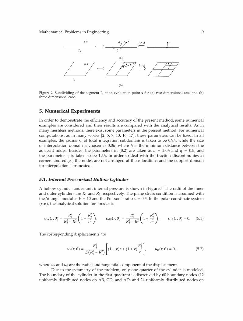
where u∗(x,y), t∗(x,y), and σ∗(x,y) are the fundamental solution with y and x being the fieldpoint and source point, respectively; NΓ is the number of the segments which compose thewhole boundary. Since every segment can be represented by a unit sector or square in theparametric space, the integrals on each segment in (4.5) and (4.6) can be computed easily.Here, an adaptive technique is developed to compute these integrals on the segment. In thistechnique, the unit sector is first divided into four equal quarters, as shown in Figure 2.Then, for each quarter, we compute the diagonal length, l, and the distance between theevaluation point and the center of the quarter, d. If l < d, this quarter is considered as aregular integration segment. Otherwise, it will be further divided into subquarters, and thisprocess goes on, until all segments become regular. Finally, Gaussian quadrature is appliedfor all segments. This adaptive scheme is very accurate even when the evaluation point isvery close to the boundary. It should be pointed out that the segments are in the parametricspace and are not like the boundary element in the BEM.

From the above discussion, it can be concluded that all integrations are computedalong the boundary only and that no boundary elements are used both for interpolation andintegration purposes. Thus, the present numerical method is truly meshless and boundary-only.


xd

l

x

Γi

x l ≥ d

(a)

Γi

xd l l ≥ d

(b)

Figure 2: Subdividing of the segment Γi at an evaluation point x for (a) two-dimensional case and (b)three-dimensional case.

5. Numerical Experiments

In order to demonstrate the efficiency and accuracy of the present method, some numericalexamples are considered and their results are compared with the analytical results. As inmany meshless methods, there exist some parameters in the present method. For numericalcomputations, as in many works [2, 5, 7, 13, 16, 17], these parameters can be fixed. In allexamples, the radius ri, of local integration subdomain is taken to be 0.9h, while the sizeof interpolation domain is chosen as 3.0h, where h is the minimum distance between theadjacent nodes. Besides, the parameters in (3.2) are taken as c = 2.0h and q = 0.5, andthe parameter ci is taken to be 1.5h. In order to deal with the traction discontinuities atcorners and edges, the nodes are not arranged at these locations and the support domainfor interpolation is truncated.

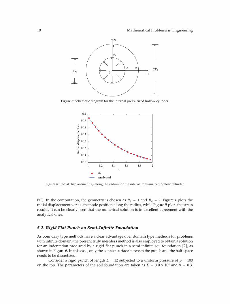
5.1. Internal Pressurized Hollow Cylinder

A hollow cylinder under unit internal pressure is shown in Figure 3. The radii of the innerand outer cylinders are R1 and R2, respectively. The plane stress condition is assumed withthe Young’s modulus E = 10 and the Poisson’s ratio ν = 0.3. In the polar coordinate system(r, θ), the analytical solution for stresses is

σrr(r, θ) =R2

1

R22 − R2

1

(

1 − R22

r2

)

, σθθ(r, θ) =R2

1

R22 − R2

1

(

1 +R2

2

r2

)

, σrθ(r, θ) = 0. (5.1)

The corresponding displacements are

ur(r, θ) =R2

1

E(R2

2 − R21

)

[

(1 − ν)r + (1 + ν)R2

2

r

]

, uθ(r, θ) = 0, (5.2)

where ur and uθ are the radial and tangential component of the displacement.Due to the symmetry of the problem, only one quarter of the cylinder is modeled.

The boundary of the cylinder in the first quadrant is discretized by 60 boundary nodes (12uniformly distributed nodes on AB, CD, and AD, and 24 uniformly distributed nodes on


A

0B

D

C

2R22R1x1

x2

Figure 3: Schematic diagram for the internal pressurized hollow cylinder.

1 1.2 1.4 1.6 1.8 20.13

0.14

0.15

0.16

0.17

0.18

0.19

0.2

Analytical

r

ur

Rad

ial d

ispl

acem

entu

r

Figure 4: Radial displacement ur along the radius for the internal pressurized hollow cylinder.

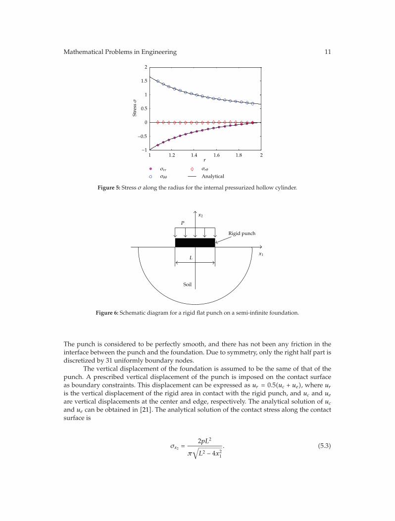
BC). In the computation, the geometry is chosen as R1 = 1 and R2 = 2. Figure 4 plots theradial displacement versus the node position along the radius, while Figure 5 plots the stressresults. It can be clearly seen that the numerical solution is in excellent agreement with theanalytical ones.

5.2. Rigid Flat Punch on Semi-Infinite Foundation

As boundary type methods have a clear advantage over domain type methods for problemswith infinite domain, the present truly meshless method is also employed to obtain a solutionfor an indentation produced by a rigid flat punch in a semi-infinite soil foundation [2], asshown in Figure 6. In this case, only the contact surface between the punch and the half-spaceneeds to be discretized.

Consider a rigid punch of length L = 12 subjected to a uniform pressure of p = 100on the top. The parameters of the soil foundation are taken as E = 3.0 × 104 and ν = 0.3.


1 1.2 1.4 1.6 1.8 2−1

−0.5

0

0.5

1

1.5

2

Analytical

σrr

σθθ

σrθ

Stre

ssσ

r

Figure 5: Stress σ along the radius for the internal pressurized hollow cylinder.

Rigid punch

x1

Soil

L

P

x2

Figure 6: Schematic diagram for a rigid flat punch on a semi-infinite foundation.

The punch is considered to be perfectly smooth, and there has not been any friction in theinterface between the punch and the foundation. Due to symmetry, only the right half part isdiscretized by 31 uniformly boundary nodes.

The vertical displacement of the foundation is assumed to be the same of that of thepunch. A prescribed vertical displacement of the punch is imposed on the contact surfaceas boundary constraints. This displacement can be expressed as ur = 0.5(uc + ue), where ur

is the vertical displacement of the rigid area in contact with the rigid punch, and uc and ue

are vertical displacements at the center and edge, respectively. The analytical solution of uc

and ue can be obtained in [21]. The analytical solution of the contact stress along the contactsurface is

σx2 =2pL2

π√L2 − 4x2

1

. (5.3)


0 1 2 3 4 5 60

200

400

600

800

1000

Analytical

σx2

σx

2

x1

Figure 7: Contact stress on the contact surface between the punch and foundation.

x3

x

a

P

b

2

x1

Figure 8: Schematic diagram for the three-dimensional Lame problem.

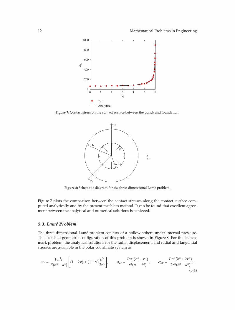
Figure 7 plots the comparison between the contact stresses along the contact surface com-puted analytically and by the present meshless method. It can be found that excellent agree-ment between the analytical and numerical solutions is achieved.

5.3. Lame Problem

The three-dimensional Lame problem consists of a hollow sphere under internal pressure.The sketched geometric configuration of this problem is shown in Figure 8. For this bench-mark problem, the analytical solutions for the radial displacement, and radial and tangentialstresses are available in the polar coordinate system as

ur =Pa3r

E(b3 − a3)

[

(1 − 2ν) + (1 + ν)b3

2r3

]

, σrr =Pa3(b3 − r3)

r3(a3 − b3), σθθ =

Pa3(b3 + 2r3)

2r3(b3 − a3),

(5.4)


1 1.5 2 2.5 3 3.5 4−8

−6

−4

−2

0

2

4

6

Analyticalσrr

σθθ

r

ur

ur,σ

rran

dσθθ

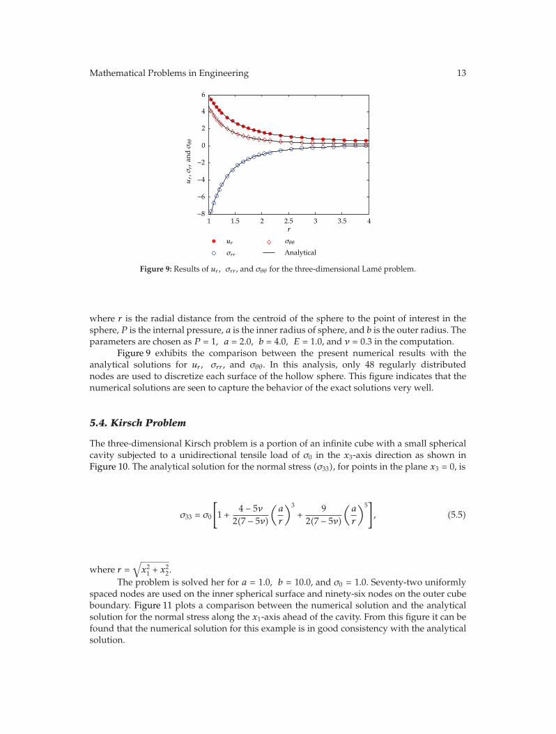
Figure 9: Results of ur , σrr , and σθθ for the three-dimensional Lame problem.

where r is the radial distance from the centroid of the sphere to the point of interest in thesphere, P is the internal pressure, a is the inner radius of sphere, and b is the outer radius. Theparameters are chosen as P = 1, a = 2.0, b = 4.0, E = 1.0, and ν = 0.3 in the computation.

Figure 9 exhibits the comparison between the present numerical results with theanalytical solutions for ur , σrr , and σθθ. In this analysis, only 48 regularly distributednodes are used to discretize each surface of the hollow sphere. This figure indicates that thenumerical solutions are seen to capture the behavior of the exact solutions very well.

5.4. Kirsch Problem

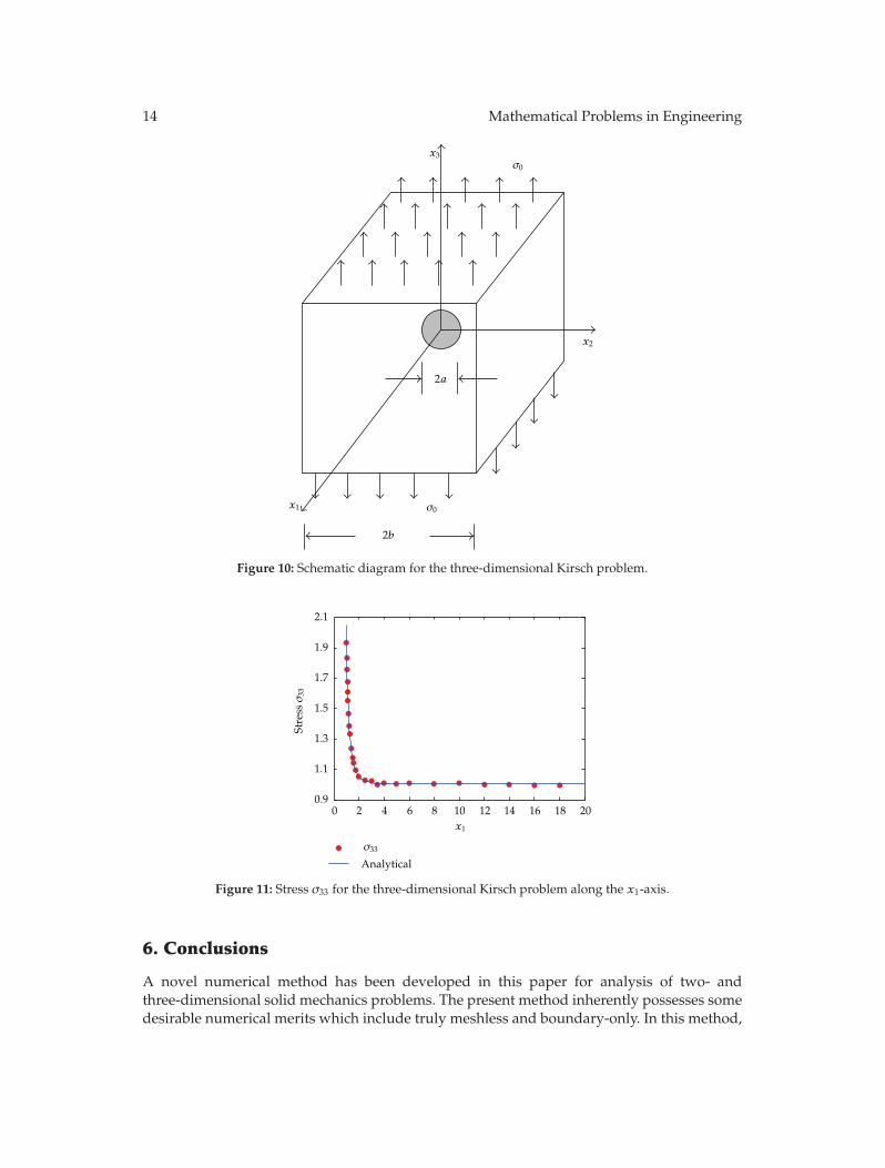
The three-dimensional Kirsch problem is a portion of an infinite cube with a small sphericalcavity subjected to a unidirectional tensile load of σ0 in the x3-axis direction as shown inFigure 10. The analytical solution for the normal stress (σ33), for points in the plane x3 = 0, is

σ33 = σ0

[

1 +4 − 5ν

2(7 − 5ν)

(a

r

)3

+9

2(7 − 5ν)

(a

r

)5]

, (5.5)

where r =√x2

1 + x22.

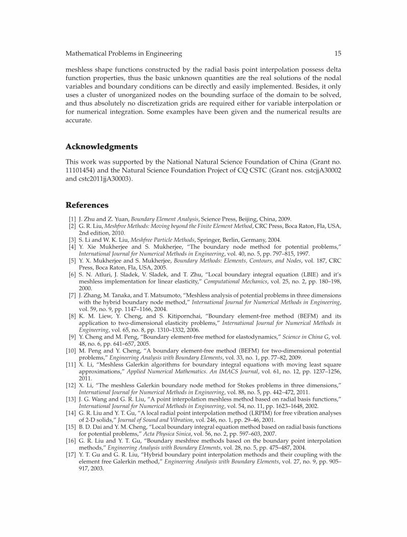
The problem is solved her for a = 1.0, b = 10.0, and σ0 = 1.0. Seventy-two uniformlyspaced nodes are used on the inner spherical surface and ninety-six nodes on the outer cubeboundary. Figure 11 plots a comparison between the numerical solution and the analyticalsolution for the normal stress along the x1-axis ahead of the cavity. From this figure it can befound that the numerical solution for this example is in good consistency with the analyticalsolution.


2a

2b

x2

x1

x3

σ0

σ0

Figure 10: Schematic diagram for the three-dimensional Kirsch problem.

0 2 4 6 8 10 12 14 16 18 200.9

1.1

1.3

1.5

1.7

1.9

2.1

Analytical

Stre

ssσ

33

σ33

x1

Figure 11: Stress σ33 for the three-dimensional Kirsch problem along the x1-axis.

6. Conclusions

A novel numerical method has been developed in this paper for analysis of two- andthree-dimensional solid mechanics problems. The present method inherently possesses somedesirable numerical merits which include truly meshless and boundary-only. In this method,


meshless shape functions constructed by the radial basis point interpolation possess deltafunction properties, thus the basic unknown quantities are the real solutions of the nodalvariables and boundary conditions can be directly and easily implemented. Besides, it onlyuses a cluster of unorganized nodes on the bounding surface of the domain to be solved,and thus absolutely no discretization grids are required either for variable interpolation orfor numerical integration. Some examples have been given and the numerical results areaccurate.

Acknowledgments

This work was supported by the National Natural Science Foundation of China (Grant no.11101454) and the Natural Science Foundation Project of CQ CSTC (Grant nos. cstcjjA30002and cstc2011jjA30003).

References

[1] J. Zhu and Z. Yuan, Boundary Element Analysis, Science Press, Beijing, China, 2009.[2] G. R. Liu, Meshfree Methods: Moving beyond the Finite Element Method, CRC Press, Boca Raton, Fla, USA,

2nd edition, 2010.[3] S. Li and W. K. Liu, Meshfree Particle Methods, Springer, Berlin, Germany, 2004.[4] Y. Xie Mukherjee and S. Mukherjee, “The boundary node method for potential problems,”

International Journal for Numerical Methods in Engineering, vol. 40, no. 5, pp. 797–815, 1997.[5] Y. X. Mukherjee and S. Mukherjee, Boundary Methods: Elements, Contours, and Nodes, vol. 187, CRC

Press, Boca Raton, Fla, USA, 2005.[6] S. N. Atluri, J. Sladek, V. Sladek, and T. Zhu, “Local boundary integral equation (LBIE) and it’s

meshless implementation for linear elasticity,” Computational Mechanics, vol. 25, no. 2, pp. 180–198,2000.

[7] J. Zhang, M. Tanaka, and T. Matsumoto, “Meshless analysis of potential problems in three dimensionswith the hybrid boundary node method,” International Journal for Numerical Methods in Engineering,vol. 59, no. 9, pp. 1147–1166, 2004.

[8] K. M. Liew, Y. Cheng, and S. Kitipornchai, “Boundary element-free method (BEFM) and itsapplication to two-dimensional elasticity problems,” International Journal for Numerical Methods inEngineering, vol. 65, no. 8, pp. 1310–1332, 2006.

[9] Y. Cheng and M. Peng, “Boundary element-free method for elastodynamics,” Science in China G, vol.48, no. 6, pp. 641–657, 2005.

[10] M. Peng and Y. Cheng, “A boundary element-free method (BEFM) for two-dimensional potentialproblems,” Engineering Analysis with Boundary Elements, vol. 33, no. 1, pp. 77–82, 2009.

[11] X. Li, “Meshless Galerkin algorithms for boundary integral equations with moving least squareapproximations,” Applied Numerical Mathematics. An IMACS Journal, vol. 61, no. 12, pp. 1237–1256,2011.

[12] X. Li, “The meshless Galerkin boundary node method for Stokes problems in three dimensions,”International Journal for Numerical Methods in Engineering, vol. 88, no. 5, pp. 442–472, 2011.

[13] J. G. Wang and G. R. Liu, “A point interpolation meshless method based on radial basis functions,”International Journal for Numerical Methods in Engineering, vol. 54, no. 11, pp. 1623–1648, 2002.

[14] G. R. Liu and Y. T. Gu, “A local radial point interpolation method (LRPIM) for free vibration analysesof 2-D solids,” Journal of Sound and Vibration, vol. 246, no. 1, pp. 29–46, 2001.

[15] B. D. Dai and Y. M. Cheng, “Local boundary integral equation method based on radial basis functionsfor potential problems,” Acta Physica Sinica, vol. 56, no. 2, pp. 597–603, 2007.

[16] G. R. Liu and Y. T. Gu, “Boundary meshfree methods based on the boundary point interpolationmethods,” Engineering Analysis with Boundary Elements, vol. 28, no. 5, pp. 475–487, 2004.

[17] Y. T. Gu and G. R. Liu, “Hybrid boundary point interpolation methods and their coupling with theelement free Galerkin method,” Engineering Analysis with Boundary Elements, vol. 27, no. 9, pp. 905–917, 2003.


[18] X. Li, J. Zhu, and S. Zhang, “A hybrid radial boundary node method based on radial basis pointinterpolation,” Engineering Analysis with Boundary Elements, vol. 33, no. 11, pp. 1273–1283, 2009.

[19] T. G. B. De Fiigueiredo, ANew Boundary Element Formulation in Engineering, Springer, Berlin, Germany,1991.

[20] M. A. Golberg, C. S. Chen, and H. Bowman, “Some recent results and proposals for the use of radialbasis functions in the BEM,” Engineering Analysis with Boundary Elements, vol. 23, no. 4, pp. 285–296,1999.

[21] S. P. Timoshenko and J. N. Goodier, Theory of Elasticity, McGraw-Hill, New York, NY, USA, 3rd edition,1970.

Submit your manuscripts athttp://www.hindawi.com

Hindawi Publishing Corporationhttp://www.hindawi.com Volume 2014

MathematicsJournal of


Mathematical Problems in Engineering

Hindawi Publishing Corporationhttp://www.hindawi.com

Differential EquationsInternational Journal of

Volume 2014

Applied MathematicsJournal of


Probability and StatisticsHindawi Publishing Corporationhttp://www.hindawi.com Volume 2014

Journal of


Mathematical PhysicsAdvances in

Complex AnalysisJournal of


OptimizationJournal of


CombinatoricsHindawi Publishing Corporationhttp://www.hindawi.com Volume 2014

International Journal of


Operations ResearchAdvances in

Journal of


Function Spaces

Abstract and Applied AnalysisHindawi Publishing Corporationhttp://www.hindawi.com Volume 2014

International Journal of Mathematics and Mathematical Sciences


The Scientific World JournalHindawi Publishing Corporation http://www.hindawi.com Volume 2014


Algebra

Discrete Dynamics in Nature and Society



Decision SciencesAdvances in

Discrete MathematicsJournal of

Hindawi Publishing Corporationhttp://www.hindawi.com

Volume 2014 Hindawi Publishing Corporationhttp://www.hindawi.com Volume 2014

Stochastic AnalysisInternational Journal of

Documents

Research Article Numerical Solution of Solid Mechanics Problems