Research Article MODELING AND MODEL PREDICTIVE …

705

Sigma J Eng & Nat Sci 37 (3), 2019, 705-722

Research Article

MODELING AND MODEL PREDICTIVE CONTROL OF A MICROTURBINE

GENERATION SYSTEM FOR STAND-ALONE OPERATION

Pouyan ASGHARIAN*1, Reza NOROOZIAN

2

1Department of Electrical Engineering, Faculty of Engineering, University of Zanjan, Zanjan, IRAN;

ORCID: 0000-0003-2993-8409 2Department of Electrical Engineering, Faculty of Engineering, University of Zanjan, Zanjan, IRAN;

ORCID: 0000-0001-8085-3860

Received: 18.09.2018 Accepted: 02.08.2019

ABSTRACT

Among a variety of Distributed Generations (DGs), microturbine (MT) generation (MTG) systems are known as highly reliable and efficient sources. The main application of MT include peak shaving, emergency power

and remote power in supplying industrial and domestic loads. The MT should support demands in any

conditions, which requires its proper control. Therefore, system accuracy and flexible management is crucial issue.

Today, Model Predictive Control (MPC) is one of the effective methods for controlling different types of

converters. Use of MPC in MTG leads to higher adaptability, outputs precise adjustment and suitable power flow.

In this paper, the MPC method is applied to control MTG's inverter irrespective of load type. Moreover, active

rectifier is used for proper DC-link voltage regulation. The simulation results indicate MPC appropriate performance to control high-frequency MT in stand-alone mode for various scenarios. In other words,

proposed system can operate with constant, variable, non-linear and unbalance loads and output three-phase

voltages are not affected by these factors. Keywords: Microturbine generation system, model predictive control, stand-alone operation, control of

voltage amplitude and frequency, controlled rectifier.

1. INTRODUCTION

Over the past decade, researches have been trying to analyze various types of DG such as

wind turbine (WT), microturbine (MT), photovoltaic (PV) and fuel cell in grid-connected or

stand-alone modes. It is widely accepted that MTG system is one of the most suitable means in

this area.

Because of the MTs inherent characteristics, they are used in a variety of, sometimes

challenging applications [1]. The MT should follow load variations to properly supply demands,

so load-following performance is a major issue [2].

The MTG dynamic modeling and its operation analysis in stand-alone or grid-connected

modes are solved problems [3-8]. Mentioned references are employed classical Proportional-

* Corresponding Author: e-mail: [email protected], tel: +0989117226519

Sigma Journal of Engineering and Natural Sciences

Sigma Mühendislik ve Fen Bilimleri Dergisi

706

Integral (PI) based control method in both modes. New methods in this area have helped the MTG

to operate properly. For example, modeling and controlling GAST based MT with active power is

an appropriate method [9] for connecting to network.

Simultaneous performance (grid-connected/stand-alone) of the MTG with a novel passive

filter called Remover Ripple Circuit (RRC) has been presented in [10] as a new MTG operational

aspect. The dynamic modeling and comprehensive load-following performance analysis of a split-

shaft MT has been illustrated in [11].

Use of algorithms and control methods can be useful. Detailed dynamic modeling based on

MPC [12] and differential evolutionary algorithm [13] are presented to improve the MTG

performance.

Hybrid energy systems (especially renewable generation) with the MTG [14-17] are an

efficient strategy to generate highly reliable power for consumers. The erratic nature of renewable

energies requires a quick and highly reliable source.

In the mentioned papers, the MTG stand-alone or grid-connected modes has been investigated

for various operational conditions and all of them used classical control methods. With respect to

the MT applications, it is sometimes supplies nonlinear or unbalanced loads, so more adaptability

is required and demand response in any situation is as its challenges. The MPC is one of the most

popular method that offers more flexibility than classic methods.

The use of MPC in converters has increased and a general overview of applications of this

method for power electronic converters is presented in [18]. The MPC current control for three-

phase inverters is investigated in [19-22] and MPC voltage control for Uninterruptible Power

Supplies (UPS) is illustrated in [23]. Literature reviews confirm usefulness of the MPC for

converters control.

In this paper, MPC method is applied to precisely control of a MT. In stand-alone mode, the

MTG must regulate output voltage as well as frequency at desirable value under any operating

conditions, regardless of the load (consumers) types. Interface converter is a controlled rectifier so

as to achieve higher adaptability and three-phase inverter is controlled by MPC. Different load

types as four scenarios are examined in stand-alone mode. The MT with proposed methods has

quick response to demands and it adjusts three-phase output voltages under each condition

properly.

The rest of this paper is organized as follows: Section 2 briefly explains the MTG system,

Sections 3 and 4 are dedicated to MTG modeling and control configuration for active rectifier as

well as three-phase inverter, respectively. Finally, the simulation results and conclusion are

presented in Sections 5 and 6, respectively.

2. MICROTURBINE SYSTEM

MTs are indeed small gas turbines operating based on the Brayton thermodynamic cycle [3].

Their output power ranges from 25 kW to 1 MW and their efficiency is about 20-30%; however,

an efficiency of over 80% will be possible with Combined Heat and Power (CHP) [1, 3].

Generally, MTGs offer advantages including compact size, low initial and maintenance cost,

high reliability, control simplicity, and low emission level as well as the potential of operation

with various fuels such as natural gas, diesel, propane, kerosene, and biogas [3, 10]. Due to the

mentioned advantages and potential merits of MTs, they can be used in many applications

including peak shaving, base load, and transportation systems [1, 3].

P. Asgharian, R. Noroozian / Sigma J Eng & Nat Sci 37 (3), 705-722, 2019

707

Figure 1. The MTG system controlled by MPC

MT’s production system is similar to that of gas turbine. The main components include

compressor, combustion chamber, turbine, recuperator, and Permanent Magnet Synchronous

Generator (PMSG) [12].

First, the fresh air is drawn in to a compressor, which increases the air pressure. Afterwards,

the compressed air mixes with fuel (e.g. natural gas) to raise its temperature and pressure. Then,

the hot air expands through a turbine, which eventually makes PMSG rotate fast, thereby

providing electric power. The recuperator is employed to increase the efficiency of this cycle [10].

Recuperator is actually a heat exchanger which transfers heat from output hot gases to the

compressed air, resulting in less fuel consumption [5].

Figure 2. The MT dynamic model

MTG System

Inverter

DC/AC

PMSG

CompressorTurbine

Fuel

Combustor

Compressed

Air Ambient

Air

Recuperator

Predictive

Model

Minimization

of Cost

Function J

Exhaust

7

Predictive Controller

LC Filter

Rectifier

AC/DC

Voltage

&

current

meter

Load

abc/dq0

PI

PLL

PI

dq0/abcPI

( )cV k

( )Li k

( )ref

cV k

( 1)cV k

aS bScS

dcV

Li

cV

oi

abcv abci

dcV

t

t

ref

dcV

qi

di

ref

qI

qv

dv

0 0v

Rectifier control

1

0.01

0.23

0.8

950

+ -

+ +

+ -

+ +

+ -

Min ×

0.77

100

s

Wm (p.u)

Tm

Max

Min

Speed Ref.

(p.u)

Speed

Governor

Acc. Ref.

(p.u/sec)

Accelaration

Control

VCE

Minimum

Fuel Flow

Valve

Positioner

Fuel systemCombustor

Delay

Transfer

Delay

Radiation Shield

Thermocouple

Temperature Ref.

(°F)

Temperature

Control

Speed Controller

Temperature Controller

Fuel System

Compressor- Turbine Package

Acceleration

Controllerdu/dt

1

0.2s+1

1

0.4s+1

1

0.05s+1

3.3s+1

450s

1

2.5s+1

0.2

15s+1

25(0.4s+1)

0.05s+1

f1(TR,Wm,Wf)

Wf

TR

f2(Wt,Wm)

Wt

Modeling and Model Predictive Control of a … / Sigma J Eng & Nat Sci 37 (3), 705-722, 2019

708

There are two types of MTs based on how the above equipment is mounted, namely single-

shaft and split-shaft [3]. In the case of single-shaft, all equipment is mounted on a shaft and due to

the very high rotation speed, the output frequency is about 1-4 kHz. In the split-shaft model,

however, there are two turbines and two separate parts which are connected through a gear. The

output frequency is about 50-60 Hz and there is no need for power electronic interface [12].

Single-shaft MT is more common owing to its less maintenance and lubrication requirements.

Typically, due to their simplicity and low cost, AC-DC-AC power electronic converters are

employed, which first convert the high frequency voltage to the DC voltage using rectifier and

then convert it back again to the desired AC voltage (50 or 60 Hz) with the desired frequency and

domain using an inverter. These types of converters are called double conversion systems.

3. MICROTURBINE GENERATION SYSTEM MODELING

Fig. 1 shows a single-shaft MT in stand-alone mode that is controlled by MPC method. The

MTG output is connected to AC-DC-AC interface that inverter is controlled by MPC. Load model

is not considered and hence in any situation, sinusoidal voltage with 50 Hz frequency will be

generated. Voltage and current of the LC filter is used as MPC inputs to produce low harmonic

voltage as well as low frequency fluctuations.

3.1. MT modeling

As mentioned previously, the single-shaft MT consists of compressor, combustor, turbine,

PMSG and recuperator in the format of five controller parts. Dynamic model of a MT is shown in

Fig. 2 including speed control, acceleration control, fuel system, temperature control and turbine

dynamics.

Speed control operates based on error between reference speed (1 per unit) and rotor speed. A

lead-lag transfer function or Proportional-Integral-Derivative (PID) controller is used to model

speed governor [5]. In this paper, a lead-lag transfer function with constant values is considered.

0.4 1(25 ) (1 )

0.05 1m

sGov W

s

(1)

Where Gov is speed controller output, Wm is PMSG rotor speed. Acceleration control is used

to limit increase of rate of rotor speed at stat-up of the MT. This block can be ignored when the

rotor speed is near the rated speed [10].

Control of turbine exhaust at a predetermined firing temperature is done by temperature

control. Temperature control consists of thermocouple and radiation shield series blocks. The

output of thermocouple is compared with reference temperature (950 °F). When the thermocouple

output exceeds the reference temperature, a negative difference cause to reduce temperature [3].

The exhaust temperature characteristic is as follows:

1950 550(1 ) 700(1 )f

m fW W (2)

Where Wf is fuel system output (after time delays).

Outputs of the speed governor, acceleration control and temperature control are entered to

Min block to achieve the least value. Output signal (VCE) is passed through a limiter to enter to

fuel system. Limiter has an important role to maintain fuel demand as well as fire in a desirable

condition. VCE is scaled by 0.77 and offset by 0.23 that represents fuel flow at no load condition.

Gas turbine requires 23% fuel at no load condition and this is a major deficiency of them [3].

Fuel system consists of two series blocks which are valve positioner and actuator. There are

two times delay after fuel system. One is corresponding to combustor delay and another relates to

flow transferring.


709

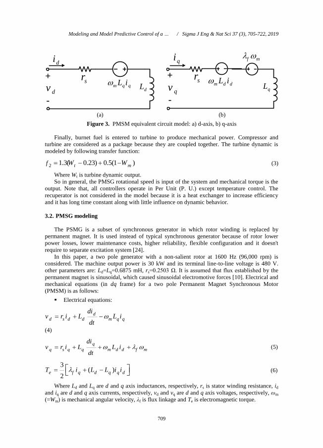
(a) (b)

Figure 3. PMSM equivalent circuit model: a) d-axis, b) q-axis

Finally, burnet fuel is entered to turbine to produce mechanical power. Compressor and

turbine are considered as a package because they are coupled together. The turbine dynamic is

modeled by following transfer function:

2 1.3( 0.23) 0.5(1 )t mf W W (3)

Where Wt is turbine dynamic output.

So in general, the PMSG rotational speed is input of the system and mechanical torque is the

output. Note that, all controllers operate in Per Unit (P. U.) except temperature control. The

recuperator is not considered in the model because it is a heat exchanger to increase efficiency

and it has long time constant along with little influence on dynamic behavior.

3.2. PMSG modeling

The PSMG is a subset of synchronous generator in which rotor winding is replaced by

permanent magnet. It is used instead of typical synchronous generator because of rotor lower

power losses, lower maintenance costs, higher reliability, flexible configuration and it doesn't

require to separate excitation system [24].

In this paper, a two pole generator with a non-salient rotor at 1600 Hz (96,000 rpm) is

considered. The machine output power is 30 kW and its terminal line-to-line voltage is 480 V.

other parameters are: Ld=Lq=0.6875 mH, rs=0.2503 Ω. It is assumed that flux established by the

permanent magnet is sinusoidal, which caused sinusoidal electromotive forces [10]. Electrical and

mechanical equations (in dq frame) for a two pole Permanent Magnet Synchronous Motor

(PMSM) is as follows:

Electrical equations:

dd s d d m q q

div r i L L i

dt

(4)

q

q s q q m d d f m

div r i L L i

dt (5)

3( )

2e f q d q q dT i L L i i (6)

Where Ld and Lq are d and q axis inductances, respectively, rs is stator winding resistance, id

and iq are d and q axis currents, respectively, vd and vq are d and q axis voltages, respectively, ωm

(=Wm) is mechanical angular velocity, λf is flux linkage and Te is electromagnetic torque.

+

-

+

-dv

di

srm q qL i

dLqv

qi

srm d dL i

f m

qL


710

Mechanical equations:

mm

d

dt

(7)

1m

e m m

dT T F

dt J

(8)

Where J is rotor and load inertia, F is rotor and load combined viscous friction, Tm is

mechanical torque and θm is rotor angular position.

According to mentioned equations, equivalent circuit of the PMSG is shown in Fig. 3. Note

that, mentioned equations are related to PMSM and reverse current direction along with negative

electric torque are correspond to PMSG [3].

4. CONTROL CIRCUITS

In the AC-DC-AC interface converter based on active rectifier, there are two control

circuits: One control circuit for regulating and controlling the inverter and another for

adjusting the input rectified and regulating the DC-link voltage. In this paper, the

rectifier is controlled by a control method based on PI controller and three-phase

inverter is controlled by MPC in order to supply the load properly.

A. Controlled Rectifier

Fig. 1 demonstrates the control diagram of the rectifier in the MTG. The PMSG three-phase

output voltages and currents as well as the DC-link voltage are applied as the control circuit

inputs so that desirable switching would occur. At first step, PMSG three-phase currents are

converted to dq0 frame according to the following equation and using the generator’s frequency

of output voltage:

0

cos( ) cos( 120 ) cos( 120 )2

sin( ) sin( 120 ) sin( 120 )3

1 1 12 2 2

d a

q b

c

i t t t i

i t t t i

i i

(9)

The d-axis reference current is determined based on the voltage error between DC-link

voltage and reference voltage. In this system, PI controller functions similar to the voltage

controller:

ref

d Pd v Id vi K e K e dt , ref

v dc dce V V (10)

Where, Kpd and Kld are the proportional gain and integral gain of PI controller, respectively

and ev represents the voltage error. By subtracting the currents measured from the reference

currents and throughout the PI controller, the dq0 voltages are obtained.

0

( )

( )

0

ref

d d d

ref

q q q

v PI i i

v PI i i

v

(11)

Typically, the value of q-axis reference current is considered zero. However, to manage the

output voltage, it can be constant number other than zero. Eventually, d-axis and q-axis voltages

are converted to abc variables by (12), and lead to generation of Pulse Width Modulation (PWM)

wave when compared with the carrier signal.


711

0

cos( ) sin( ) 1

cos( 120 ) sin( 120 ) 1

cos( 120 ) sin( 120 ) 1

a d

b q

c

v t t v

v t t v

v t t v

(12)

B. MPC-controlled inverter

Use of an inverter with an output LC filter causes generation of sinusoidal voltages with low

harmonics. Control of the inverter is rather complex and difficult to achieve a suitable switching

status. In this paper, the control strategy is based on controlling the load frequency and voltage. In

other words, in the MT stand-alone mode, the voltage in terms of amplitude and frequency should

be regulated under any operating conditions.

To simply use of MPC, the inverter can be modeled systemically with a limited number of

switching states [23]. No need to the load information is one of the strong points of MPC voltage

control, where regardless of the load type, a sinusoidal output voltage is generated with a

frequency of 50 Hz.

In prediction horizon Hp with the control horizon Hc, MPC functions to achieve the optimal

solution, where always Hc ≤ Hp. in any time sample, MPC predicts Hp numbers of the variable of

interest and tries to achieve it with the control attempt Hc [18].

To obtain the optimal solution, a function called cost function is defined [19]. Indeed, the

difference between the value generated by MPC and the desirable value of the variable

determines the cost function g, where the aim is to have the output follow the desired value.

Typically, modeling is done in discrete state and within a short sampling time.

1) The cost function

The selected cost function is used in the alpha-beta transformation and operated based on the

subtraction of the predicted voltage and reference voltage. The reference voltage is a sinusoidal

voltage with the frequency of 50 Hz. In this section, the optimal voltage is the one which

minimizes the cost function and indeed well follows the reference value. The following shows the

cost function:

ref p ref p

c c c cJ V V V V (13)

Where, p

cV and p

cV are the real and imaginary parts of the output voltage p

cV ,

respectively. Also, ref

cV and ref

cV represent the real and imaginary parts of the reference voltage

ref

cV respectively. It is assumed that the reference voltage has no sensible changes and is constant

between two consecutive samplings.

2)Inverter model

A three-phase inverter with LC filter and unknown load is shown in Fig. 4, based on which the

mathematical relations have been presented.

In order to prevent the phases from becoming short-circuit, at any moment, one switch should

be turn on in each leg of the inverter. Indeed, the switching states is as follows:

1 2 3

4 5 6

1 , ,

0 , , i

if S S S onS

if S S S on

, i=a, b, c (14)

Since at any moment, one switch should be turn on in each inverter’s leg. Thus, (14) can be

rewritten as a vector:


712

Figure 4. Three-phase inverter with LC filter and unknown load

22( )

3a b cS S aS a S (15)

Where, 1 120a . Similarly, the output voltage of the inverter can be stated as a vector as

well as a function of phase-voltages:

22

3i aN bN cNV v av a v (16)

Where, vaN, vbN, and vcN are the phase voltages to ground. The inverter’s switching strategy

causes generation of different voltages from the input to the output. Therefore, the vector of the

output voltage of inverter can be considered as the vector multiplication of constant input voltage

and switching vector as:

i dcV V S (17)

Where, Vdc is the DC-link voltage of the input. According to (15) and (17), it can be

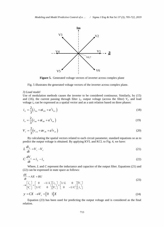
concluded that eight switching states and thus eight output voltage vectors will be generated for

the inverter. Table 1 shows the output voltages resulting from the different switching states. Note

that V0=V7, and hence per eight switching states, there are seven different voltage vectors.

Table 1. Switching state and voltage vectors

Sa Sb Sc Voltage vector (V)

0 0 0 0 0V

1 0 0 12

3 dcV V

1 1 0 231

3 3dc dcV V j V

0 1 0 331

3 3dc dcV V j V

0 1 1 42

3 dcV V

0 0 1 531

3 3dc dcV V j V

1 0 1 631

3 3dc dcV V j V

1 1 1 7 0V

S1 S2 S3

S4 S5 S6

ab

c

N

+

Vdc

-VcN

VbNVaN

iL io

Vc

Unknown

Load

L

C


713

Figure 5. Generated voltage vectors of inverter across complex plane

Fig. 5 illustrates the generated voltage vectors of the inverter across complex plane.

3) Load model

Use of modulation methods causes the inverter to be considered continuous. Similarly, by (15)

and (16), the current passing through filter iL, output voltage (across the filter) Vc, and load

voltage io can be expressed as a spatial vector and as a unit relation based on three phases:

22

3L La Lb Lci i ai a i (18)

22

3o oa ob oci i ai a i (19)

22

3c ca cb ccV v a vv a (20)

By calculating the spatial vectors related to each circuit parameter, standard equations so as to

predict the output voltage is obtained. By applying KVL and KCL to Fig. 4, we have:

Li c

diL V V

dt (21)

cL o

dVC i i

dt (22)

Where, L and C represent the inductance and capacitor of the output filter. Equations (21) and

(22) can be expressed in state space as follows:

0 1/ 1/ 0

1/ 0 0 1/

L iL

c oc

dXAX BU

dt

i VL Li

V iC CV

(23)

0 1cy CX V X (24)

Equation (23) has been used for predicting the output voltage and is considered as the final

relation.

Im

ReV1

V2V3

V4

V5 V6

V0,7


714

4) Discrete-time model for the prediction

In order to predict the output voltage, (23) should be rewritten as discrete for the sampling time

Ts. One of the discretization methods has been stated as below [23]; nevertheless, in MATLAB

software by specifying the state matrices and sampling time, discrete matrices can be accessed

with “c2d” command.

sAT

dA e (25)

0

sT

A

dB e Bd (26)

The discrete form of (23) is as follows:

( 1) ( ) ( )d dX k A X k B U k (27)

Voltage prediction can be done by (27). In this equation, Vc and iL, which are the voltage and

current of filter, respectively, are obtained through measurement, and Vi is specified according to

(17) and Table 1. Since the load has been considered as unknown, io can be calculated

approximately by the following relation:

( 1) ( 1) ( ( ) ( 1))o L c c

Ci k i k V k V k

T (28)

Where, k is related to the present sampling time, while k+1 is associated with the future

prediction. In each sampling, eight different output voltage are obtained per different Vi, among

which the voltage that minimizes the cost function is chosen. The MPC function flowchart in

controlling of output voltage is shown in Fig. 6.


715

Figure 6. MPC flowchart based on voltage control

5. SIMULATION RESULTS

In this paper, modeling and control of the MTG in stand-alone mode based on the MPC control

method is presented for greater flexibility. The simulation of MTG (Fig. 1) has been done in

MATLAB/Simulink environment and system parameters are given in Table 2.

To further investigate the mentioned control method, four different scenarios is presented for

load including constant RL load, variable RL load, imbalanced load and nonlinear load. The

amplitude of the reference voltage is 400 V with the frequency of 50 Hz, and also the MTG

values are measured in per unit (P. U.).

Table 2. Studied system parameters

Parameter Value

DC-link capacitor 4500 µF

Filter inductance 3 mH

Filter capacitor 50 µF

Sampling time 25 µs

Microturbine output power 30 kW

Load ZL=50+j31.416

Startup

Measure

Store Optimal

Values

No

Apply optimal

vector V(k)

Yes

Wait for next

sampling instant

( ), ( )c LV k i k

( 1) ( 1) ( ) ( 1)o L c c

Ci k i k V k V k

T

0X

1X X

21 22

21 22

( 1) ( ) ( )

( ) ( )

c d L d c

d i d o

V k A i k A V k

B V k B i k

ref p ref p

c c c cg V V V V

8?X


716

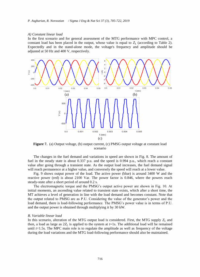
A) Constant linear load

In the first scenario and for general assessment of the MTG performance with MPC control, a

constant load has been placed in the output, whose value is equal to ZL (according to Table 2).

Expectedly and in the stand-alone mode, the voltage's frequency and amplitude should be

adjusted at 50 Hz and 400 V, respectively.

(a) (b)

(c)

Figure 7. (a) Output voltage, (b) output current, (c) PMSG output voltage at constant load

scenario

The changes in the fuel demand and variations in speed are shown in Fig. 8. The amount of

fuel in the steady state is about 0.337 p.u. and the speed is 0.994 p.u., which reach a constant

value after going through a transient state. As the output load increases, the fuel demand signal

will reach permanence at a higher value, and conversely the speed will reach at a lower value.

Fig. 9 shows output power of the load. The active power (blue) is around 3400 W and the

reactive power (red) is about 2100 Var. The power factor is 0.846, where the powers reach

steady-state after a short period of around 0.2 s.

The electromagnetic torque and the PMSG’s output active power are shown in Fig. 10. At

initial moments, an ascending value related to transient state exists, which after a short time, the

MT achieves a level of generation in line with the load demand and becomes constant. Note that

the output related to PMSG are as P.U. Considering the value of the generator’s power and the

load demand, there is load-following performance. The PMSG’s power value is in terms of P.U.

and the output power is obtained through multiplying it by 30 kW.

B. Variable linear load

In this scenario, alteration of the MTG output load is considered. First, the MTG supply ZL and

then, a load as large as 2ZL is applied to the system at t=1s. The additional load will be remained

until t=1.5s. The MPC main role is to regulate the amplitude as well as frequency of the voltage

during the load variations and the MTG load-following performance should also be maintained.


717

(a) (b)

Figure 8. (a) Fuel demand signal, (b) MT output speed at constant load scenario

Figure 9. Output powers at constant load scenario

(a) (b)

Figure 10. (a) PMSG electromagnetic torque, (b) PMSG active power at constant load scenario

Fig. 11 shows the three-phase output voltage and current at the moment of load variation. As

can be seen, the voltage amplitude remains constant during the variation and no change occurs in

the value of operating frequency. Therefore, voltage is tracked sinusoidal reference properly.

The output current during load variation is shown in Fig. 11(b). As the load rise, the current’s

amplitude increases from 6.45 to around 10 A in a short time and maintains its sinusoidal state.

(a) (b)

Figure 11. (a) Output voltage, (b) output current at variable load scenario


718

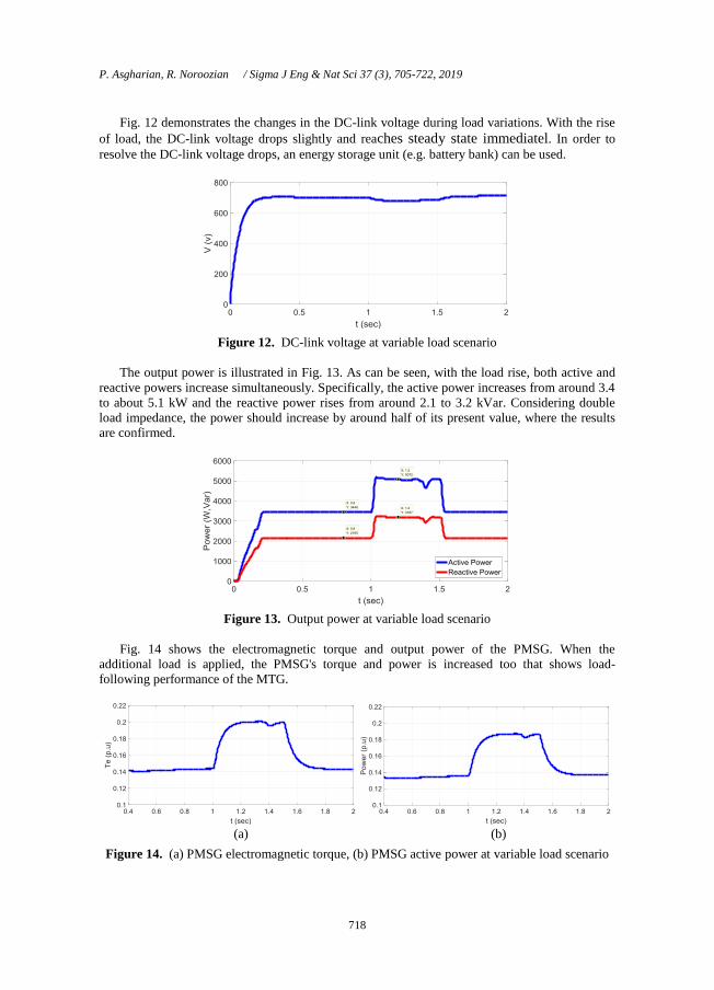
Fig. 12 demonstrates the changes in the DC-link voltage during load variations. With the rise

of load, the DC-link voltage drops slightly and reaches steady state immediatel. In order to

resolve the DC-link voltage drops, an energy storage unit (e.g. battery bank) can be used.

Figure 12. DC-link voltage at variable load scenario

The output power is illustrated in Fig. 13. As can be seen, with the load rise, both active and

reactive powers increase simultaneously. Specifically, the active power increases from around 3.4

to about 5.1 kW and the reactive power rises from around 2.1 to 3.2 kVar. Considering double

load impedance, the power should increase by around half of its present value, where the results

are confirmed.

Figure 13. Output power at variable load scenario

Fig. 14 shows the electromagnetic torque and output power of the PMSG. When the

additional load is applied, the PMSG's torque and power is increased too that shows load-

following performance of the MTG.

(a) (b)

Figure 14. (a) PMSG electromagnetic torque, (b) PMSG active power at variable load scenario


719

C) Imbalanced load

In the third scenario, the imbalanced load has been considered in the output. Different load values

are connected to each phase including phase a as large as 0.5ZL (yellow), phase b equal to ZL

(red), and phase c as large as 2ZL (blue). The MTG should have the ability of properly supplying

the imbalanced loads. This means that irrespective of the output current, a sinusoidal voltage with

a constant amplitude and frequency should feed the consumers.

The output three-phase voltage is shown in Fig. 15. In spite of imbalanced load, the output

voltage has a constant amplitude and frequency, and well follows the sinusoidal reference.

Figure 15. Output voltage at unbalance load scenario

Fig. 16 shows the output current in the imbalanced load state. Expectedly, the current in each

phase has different value due to various load powers, where unbalance state is clearly observed.

Figure 16. Output current at unbalance load scenario

Fig. 17 shows the inverter’s output current (i.e. iL). The currents suffer from severe imbalance,

but the voltage emerges as balanced sinusoidal in the output.

Figure 17. Inverter output current at unbalance load scenario


720

D) Nonlinear load

In the last scenario, a nonlinear load is connected to output. The nonlinear load consists of a diode

rectifier and RL load with a power of S=500+j100 VA, which generates high amount harmonics.

Fig. 18 shows the three-phase output voltages. In spite of the nonlinear load, the voltage is

generated as sinusoidal with an amplitude of 400 V and frequency of 50 Hz and minimum extent

of harmonics.

Figure 18. Output voltage at nonlinear load scenario

The output current is shown in Fig. 19, which is highly affected by harmonics and has

completely lost its sinusoidal state.

Figure 19. Output current at nonlinear load scenario

The inverter’s output current is demonstrated in Fig. 20. Nonlinear load harmonics has a

detrimental effect on the currents, though the voltage is generated as completely sinusoidal with

lowest THD.

Figure 20. Inverter output current at nonlinear load scenario


721

6. CONCLUSION

This paper presented dynamic modeling of a MTG using MPC control method in stand-alone

mode. Single-shaft MTs require interface converter due to generation of high-frequency voltages,

where AC-DC-AC configuration is selected in this paper.

The MTGs are mostly used as emergency or dispatchable sources in power system so, it is

required to generate sinusoidal voltage along with low THD irrespective of the output load types

and under any operational conditions. Accordingly, MPC method is chosen due to structure

simplicity and high flexibility. This control method is absolutely based on system model and

independent of the load type.

The simulation results indicated that MPC well regulates the output voltage in high-frequency

MTs for linear, nonlinear, imbalanced and variable loads, which results in improved stability and

dynamic responsibility. Use of MPC in MTG control is a novel and flexible method which is

investigated in this paper.

REFERENCES

[1] Breeze P. Microturbines. In: Breeze P, editor. Gas-Turbine Power Generation. 4

Netherland: Elsevier Science & Technology Books, 2016. pp. 77-82.

[2] Ismail MS, Moghavvemi M, Mahlia, TMI. Current utilization of microturbines as a part

of a hybrid system in distributed generation technology. Renewable and Sustainable

Energy Reviews 2013; 21: 142-152.

[3] Asgharian P, Noroozian R. Microturbine Generation Power Systems. In: Gharehpetian

GB, Mousavi Agah SM, editors. Distributed Generation Systems: Design, Operation and

Grid Integration. Netherland: Butterworth-Heinemann, Elsevier Science & Technology

Books, 2017. pp. 149-219.

[4] Saravanan, G, Gnanambal I. Design and Efficient Controller for Micro Turbine System.

Circuits and Systems 2016; 7: 1224-1232.

[5] S. K. nayak and D. N. Gaonkar, “Performance Study of Distributed Generation System in

Grid Connected/Isolated Modes,” Distributed Generation & Alternative Energy Journal,

vol. 29, no.1, pp. 61-80, 2014.

[6] Sarajian, S., “Design and Control of Grid Interfaced Voltage Source Inverter with Output

LCL Filter”, International Journal of Electronics Communications and Electrical

Engineering, Vol. 4, pp. 26–40, 2014.

[7] Ranjbar, M., Mohaghegh, S., Salehifar, M., Ebrahimirad, H., Ghaleh, A., “Power

Electronic Interface in a 70 kW Microturbine-Based Distributed Generation”, IEEE 2nd

Power Electronics, Drive Systems and Technologies Conference, Tehran, Iran, 2011.

[8] A. Tyagi and Y. K. Chauhan, “A Prospective on Modeling and Performance Analysis of

Micro-turbine Generation System,” presented at IEEE International Conference on

Energy Efficient Technologies for Sustainability (ICEETS), Nagercoil, India, April 10-12,

2013.

[9] Saha AK, Chowdhury S, Chowdhury SP, Crossley PA. Modeling and Performance

Analysis of a Microturbine as a Distributed Energy Resource. IEEE T ENERGY

CONVER 2009; 24: 529-538.

[10] Asgharian P, Noroozian R. Modeling and simulation of microturbine generation system

for simultaneous grid-connected/islanding operation. In: IEEE 24th Iranian Conference on

Electrical Engineering (ICEE); 10-12 May 2016; Shiraz, Iran: IEEE. pp. 1528-1533.

[11] Shankar G, Mukherjee V. Load-following performance analysis of a microturbine for

islanded and grid connected operation. INT J ELEC POWER 2014; 55: 704-713.


722

[12] Asgharian P, Noroozian R. Dynamic Modeling of a Microturbine Generation System for

Islanding Operation based on Model Predictive Control. In: 31st international Power

System Conference (PSC); 24-26 Oct. 2016; Tehran, Iran.

[13] Keshtkar, H., Solanki, J., Solanki, S. K., “Dynamic modeling, control and stability

analysis of microturbine in a microgrid”, IEEE PES T&D Conference and Exposition,

Chicago, USA, 2014.

[14] Mousavi GSM. An autonomous hybrid energy system of wind/tidal/microturbine/battery

storage. INT J ELEC POWER 2012; 43: 1144-1154.

[15] Comodi G, Renzi M, Cioccolanti L, Caresana F, Pelagalli L. Hybrid system with micro

gas turbine and PV (photovoltaic) plant: Guidelines for sizing and management strategies.

ENERGY 2015; 89: 226-235.

[16] Bakalis DP, Stamatis AG. Incorporating available micro gas turbines and fuel cell:

Matching considerations and performance evaluation. APPL ENERG 2013; 103: 607-617.

[17] Baudoin S, Vechiu L, Camblong H, Vinassa J, Barelli L. Sizing and control of a Solid

Oxide Fuel Cell/Gas microturbine hybrid power system using a unique inverter for rural

microgrid integration. APPL ENERG 2016; 176: 272-281.

[18] Kouro, S., Cortes, P., Vargas, R., “Model Predictive Control—A Simple and Powerful

Method to Control Power Converters”, IEEE Trans. Ind. Electron., Vol. 56, No. 6, pp.

1826-1838, 2009.

[19] Rodriguez, J., Cortes, P., Predictive control of power converters and electrical drives,

OMG Press, Wiley Publishing, 2012.

[20] Young, H. A., Perez, M. A., Rodriguez, J., “Analysis of Finite-Control-Set Model

Predictive Current Control with Model Parameter Mismatch in a Three-Phase Inverter”,

IEEE Trans. Ind. Electron., Vol. 63, No. 5, pp. 3100-3107, 2016.

[21] Young, H. A., Perez, M. A., Rodriguez, J., Abu-Rub, H., “Assessing Finite-Control-Set

Model Predictive Control: A Comparison with a Linear Current Controller in Two-Level

Voltage Source Inverters”, IEEE Ind. Electron. Magazine, Vol. 8, No. 1, pp. 44-52, 2014.

[22] Rodríguez, J., Pontt, J., Silva, C. A., Correa, P., Lezana, P., Cortes, P., Amman, U.,

“Predictive Current Control of a Voltage Source Inverter”, IEEE Trans. Ind. Electron.,

Vol. 54, No. 1, pp. 495-503, 2007.

[23] Cortés. P., Ortiz, G., Yuz, J. I., Rodríguez, J., Vazquez, S., Leopoldo, G., “Model

Predictive Control of an Inverter with Output LC Filter for UPS Applications”, IEEE

Trans. Ind. Electron., Vol. 56, No. 6, pp. 1875-1883, 2009.

[24] Paul Krause, Oleg Wasynczuk, Scott Sudhoff, Steven Pekarek, Analysis of electric

machinery and drive systems. Wiley-IEEE Press, 2013.


Documents

Research Article MODELING AND MODEL PREDICTIVE …