Embed Size (px)
Citation preview

Research ArticleApproximate Solutions of Delay Differential Equationswith Constant and Variable Coefficients by the EnhancedMultistage Homotopy Perturbation Method
D Olvera1 A Eliacuteas-Zuacutentildeiga1 L N Loacutepez de Lacalle2 and C A Rodriacuteguez1
1Center for Innovation in Design and Technology Tecnologico de Monterrey Campus Monterrey E Garza Sada 250164849 Monterrey NL Mexico2Department of Mechanical Engineering University of the Basque Country Alameda de Urquijo sn Bilbao 48013 Bizkaia Spain
Correspondence should be addressed to A Elıas-Zuniga aeliasitesmmx
Received 26 December 2013 Revised 21 July 2014 Accepted 16 August 2014
Academic Editor Zhichun Yang
Copyright copy 2015 D Olvera et alThis is an open access article distributed under theCreative CommonsAttribution License whichpermits unrestricted use distribution and reproduction in any medium provided the original work is properly cited
We expand the application of the enhanced multistage homotopy perturbation method (EMHPM) to solve delay differentialequations (DDEs) with constant and variable coefficients This EMHPM is based on a sequence of subintervals that provideapproximate solutions that require less CPU time than those computed from the dde23 MATLAB numerical integration algorithmsolutions To address the accuracy of our proposed approachwe examine the solutions of severalDDEs having constant and variablecoefficients finding predictions with a good match relative to the corresponding numerical integration solutions
1 Introduction
Delayed differential equations (DDEs) are used to describemany physical phenomena of interest in biology medicinechemistry physics engineering and economics among oth-ers Since the introduction of the first delayed models manypublications have appeared as summarizing theorems andhomotopy methods of solution that deal with the stabilityproperties of delayed systems (see [1ndash3] and references citedthere in)
For instance Shakeri andDehghan introduced an approachto find the solution of delay differential equations by meansof the homotopy perturbation technique (HPM) with resultsthat agree well with exact solutions [1] Wu in [2] usedthe homotopy analysis method to obtain the approximatesolution of a strong nonlinear ENSOdelayed oscillatormodelthat provides good agreement when compared to its exactsolution under the condition of 119861 = 0 Alomari andcoworkers in [3] developed an algorithm to obtain approx-imate analytical solutions for DDEs by using the homotopyanalysismethod (HAM) and themodified homotopy analysismethod (MHAM)They used their derived method to obtain
the approximate solution of various linear and nonlinearDDEs with numerical predictions that agree well with thenumerical integration solutions and they also proved thattheir derived solutions converge to the exact ones By apply-ing the homotopy perturbation method (HPM) Biazar andBehzad found approximate solutions of neutral differentialequations with proportional delays which describe well theircorresponding numerical integration solutions [4] RecentlyAnakira and co-workers in [5] extended the applicability ofthe so called optimal homotopy asymptoticmethod (OHAM)that does not depend on small or large parameters to findthe approximate analytic solution of DDEs They used theirproposed approach to compare the derived approximatesolutions of several DDEswith their exact analytical solutionswith predictions that compare well with the exact ones
On the other hand Insperger and Stepan in [6] used thesemidiscretization method to determine the stability lobes ofDDEs that model the dynamics of cutting machine opera-tions Based on the properties of the Chebyshev polynomialsButcher and coworkers in [7] developed a methodology toobtain the stability lobes of milling machine operations and
Hindawi Publishing CorporationAbstract and Applied AnalysisVolume 2015 Article ID 382475 12 pageshttpdxdoiorg1011552015382475
2 Abstract and Applied Analysis
they proved that this technique is faster than that of thefull and the semidiscretization methods since these solutiontechniques approximate the original DDEs by a series ofODEs [8]
Here in this paper we develop a generalized procedure tosolve linear and nonlinear DDEs by introducing some mod-ifications to the multistage homotopy perturbation method(MHPM) derived by Hashim and Chowdhury to obtainapproximate solutions of ordinary differential equations [9]The proposed enhanced multistage homotopy perturbationmethod (EMHPM) is based on a sequence of subintervalsthat allow us to find more accurate approximated solutionsunder a numerical-analytical procedure that requires lessCPU time when compared to the numerical integrationsolutions provided by the MATLAB dde23 algorithm writtenby Shampine and Thompson in [10] The EMHPM is basedon a homotopy function that could be divided into a linearoperator and a nonlinear operator to satisfy its assumed initialsolution This split of the homotopy function allows us tomodify the nonlinear operator to guarantee by using theenhanced homotopy perturbation method the stability ofthe proposed approximate solutions of nonlinear differentialequations [11]
To clarify our proposed method we briefly review inSection 2 some basic concepts of the homotopy perturbationmethod and then in Section 3 we introduce the EMHPMto solve DDEs The difference between the HPM and theEMHPM is discussed in Section 4 by addressing the approx-imate solutions of a nonlinear delayed differential equationwith variable coefficients Finally the general solution oftwo DDEs that describe the dynamics of two engineeringproblems by using the EMHPM is discussed in Section 5
2 Homotopy Perturbation Method
The homotopy perturbation method (HPM) is a couplingof the traditional perturbation method and homotopy intopology which eliminates the limitation of the small param-eter assumed in the perturbation methods [12] Under thisapproach a nonlinear problem can be transformed into aninfinite number of simple problems without the restrictionof having small nonlinear parameter values This homotopyperturbationmethod takes themain advantages of traditionalperturbation methods together with homotopy analysis [13ndash15]
To illustrate the basic ideas of the HPM let us considerthe following nonlinear differential equation
119860 (119906) minus 119891 (119903) = 0 119903 isin Ω (1)
with boundary conditions
119861(119906120597119906
120597119899) = 0 119903 isin Γ (2)
where 119860 is a general differential operator 119861 is a boundaryoperator 119891(119903) is a known analytic function and Γ is theboundary of the domainΩ
The operator 119860 can generally be divided into two parts 119871and119873 where 119871 involves the linear terms and119873 the nonlinearones Equation (1) therefore can be rewritten as follows
119871 (119906) + 119873 (119906) minus 119891 (119903) = 0 (3)
By the homotopy perturbation technique we construct a homo-topy V(119903 119901) Ω times [0 1] rarr R that satisfies
119867(V 119901) = 119871 (V) minus 119871 (1199060) + 119901119871 (1199060) + 119901 [119873 (V) minus 119891 (119903)] = 0(4)
where 119901 isin [0 1] is an embedding parameter and 1199060is
an initial approximation of (1) which satisfies the boundaryconditions (2) Thus from (4) we have
119867(V 0) = 119871 (V) minus 119871 (1199060) = 0
119867 (V 1) = 119860 (V) minus 119891 (119903) = 0(5)
The changing process of 119901 from zero to unity is just thatof V(119903 119901) from 119906
0(119903) to 119906(119903) In topology this is called
deformation and 119871(V) minus 119871(1199060) and 119860(V) minus 119891(119903) are called
homotopicHe in [12] uses the embedding parameter 119901 as the small
parameter and assumed that the solution of (4) can be writtenas a power series of 119901 in the form
V = V0+ 119901V1+ 1199012V2+ sdot sdot sdot (6)
By setting 119901 = 1 He obtained the approximate solution of (1)as
119906 = lim119901rarr1
= V0+ V1+ V2+ sdot sdot sdot (7)
Then this method was applied to obtain the approximatesolution of some nonlinear ordinary differential equationsvalid not only for small but also for large nonlinear parametervalues
We next will introduce an approach based on homotopymethods to obtain the solution of DDEs with constant andvariable coefficients
3 The EMHPM Methodology to Solve DDEs
TheHPM is an asymptotic method that depends on the aux-iliary linear operator form and the initial guess of the initialconditions Therefore the convergence of the approximatesolution cannot be guaranteed in some cases [16] Hashimand Chowdhury showed in [9] that the solutions obtained bythe standard HPM were not valid for large time span unlessmore terms are calculated Thus they proposed a multistagehomotopy perturbation method (MHPM) which treated theHPMalgorithm in a sequence of subintervals in an attempt toimprove the accuracy of the approximate solutions of linearand nonlinear ordinary differential equations (ODEs)
However when the MHPM is applied to obtain theapproximate solutions of ODEs which contain coefficientsas a function of time this method cannot provide accuratesolutions when Δ119905 rarr 0 In this work we introduce some
Abstract and Applied Analysis 3
modifications to the MHPM and focus on the derivation ofapproximate solutions of DDEs equations with variable coef-ficient terms This new approach is based on the enhancedmultistage homotopy perturbationmethod (EMHPM) intro-duced in [17] to obtain the solution of nonlinear ordinarydifferential equations
The EMHPM is an algorithm which approximates theHPM solution by subintervals utilizing the following trans-formation rule 119906(119905) rarr 119906
119894(119879) where 119906
119894satisfies the initial
condition 119906119894(0) = 119906
119894minus1(119905119894minus1) 119879 is a shifted time scale used
to determine the approximate solution in each subintervaland 119906
119894(119879) represents the approximate solution in the 119894th
subinterval In this case the initial suggested solution in the119894th subinterval is given by 119906
1198940(119879) = 119906
119894minus1(119905119894minus1) where 119905
119894minus1
represents the time at the end of the previous subinterval(ie the value of the approximate solution at the end of theprevious subinterval represents the initial conditions of thenext subinterval under consideration)
To apply the homotopy technique to solve delay differen-tial equations we also assume the following
(1) The linear operator119871(119906119894) represents119871(119906
119894) = (119889119889119879)119906
119894
where the assumed approximate solution 1199061198940(119879) is
set equal to the initial condition 119906119894minus1(119905119894minus1) that is
1199061198940= 119906119894minus1(119905119894minus1) To simplify the notation we let 119906
119894minus1equiv
119906119894minus1(119905119894minus1)
(2) The transformation 119879 = 119905 minus 119905119894minus1
on 0 lt 119879 le 119905119894minus 119905119894minus1
holds in the homotopy 119894-subinterval Thus higherorder equations are integratedwith respect to119879 whilethe terms related to the independent variable 119905 areassumed to remain constant
Therefore we may conclude that the 119898 order approximatesolution by applying the EMHPM can be written as
119906119894(119879 119906119894minus1) =
119898
sum
119896=0
119880119894119896(119879 119906119894minus1) (8)
where the solution 119906119894(119879 119906119894minus1) is valid only in the 119894th subin-
terval [119905119894minus1 119905119894] Hence the solution 119906(119905) on the 119894th subinterval
(119905119894minus1 119905119894] can be written as
119906 (119905) asymp 119906119894(119905 minus 119905119894minus1) (9)
with initial condition 119906119894minus1(119905119894minus1) and 119894 = 1 2 119895 Thus the
approximate solution of 119906 at the time 119905119894is given by
119906119894(119905 minus 119905119894minus1)1003816100381610038161003816119905=119905119894= 119906119894+1(119905 minus 119905119894)1003816100381610038161003816119905=119905119894= 119906119894+1(0) = 119906
119894 (10)
In summary the solution 119906(119905) for an open-closed interval(1199050 1199051] is divided into 119895 subintervals that in general are
not equally spaced [1199050 1199051] [1199051 1199052] [119905
119895minus1 119905119895] Thus the
approximated solution of 119906(119905) for the span time interval isobtained by coupling the 119906
119894(119905) solutions
4 Approximate Solutions of Some DDEs byApplying the EMHPM
In this sectionwe focus on the solution ofDDEswith constantand variable coefficients and examine the applicability of theEMHPM to find the corresponding approximate solutions
41 Delay Differential Equations with Constant CoefficientsFirst let us consider the simplest DDE of the form
(119905) + 119909 (119905 minus 120591) = 0 (11)
with initial condition 119909(0) = 119888 Here the independent vari-able 119909 is a scalar 119909(119905) isin R the dot stands for differentiationwith respect to time 119905 and 120591 is the time delay To evaluate(11) on 119886 le 119905 le 119887 the term 119909(119905 minus 120591) must represent a knownfunction 119909(119905) on [119886 minus 120591 le 119905 le 119886] For instance if 119886 = 0the solution of (11) can be obtained in the interval (0 120591] byassuming an initial function that satisfies the initial conditionBy using this solution it becomes possible to obtain thesolution of (11) in the next 119894th interval [(119894 minus 1)120591 119894120591] 119894 =2 3 119895 where 119895 is an integer number that can be chosenas 2 le 119895 le infin With this approach we can apply the HPM tofind the solution of (11) by assuming that the previous delayedfunction is 1199091205910(119879) = 119888 thus the solution for the first intervalis given by 1199091205911(119879) valid on [0 120591] In terms of (4) we nowconstruct the homotopy of (11)
119867(1198831205911 119901) =
119889
1198891198791198831205911 + 119901119909
1205910 = 0 (12)
We next substitute the first order expansion1198831205911 = 11988312059110+1199011198831205911
1
in (12) and balance the terms with identical power of 119901 toobtain the following set of linear differential equations
1199010 1198891198891198791198831205911
0= 0 119883
1205911
0(0) = 119888 = 119883
1205910(120591)
1199011 1198891198891198791198831205911
1= minus1198831205910 119883
1205911
1(0) = 0
(13)
Integration of (13) yields
1198831205911
0= 119888
1198831205911
1= minus 119888119879
(14)
Hence the first order solution of (12) is given by
1199091205911(119879) = 119888 minus 119888119879 (15)
Notice that (15) represents the exact solution of (11) on thefirst interval By following the same procedure it is easy toshow that the exact solution of (11) for the second and thirdintervals is given respectively as
1199091205912(119879) = 119888 minus 119888120591 minus 119888119879 +
1
21198881198792
1199091205913(119879) = 119888 minus 2119888120591 +
1
21198881205912minus (119888 minus 119888120591) 119879 +
1
21198881198792minus1
61198881198793
(16)
Figure 1 shows the exact solution of (11) obtained by couplingat each interval the solution obtained by following HPMprocedure for 119905 = 10120591
It is easy to show that the solution of (11) by the EMHPMcoincides with the solution obtained by using the HPM since(11) is a delay differential equation with constant coefficients
4 Abstract and Applied Analysis
0 1 2 3 4 5 6 7 8 9 10
00
0505
11
Time t
HPM by intervals
minus05minus05
Am
plitu
dex
Figure 1 Exact solution of (11) obtained by using theHPMand 120591 = 1
42 Delay Differential Equations with Variable CoefficientsWe next show how the EMHPM approach can be applied toobtain the approximate solution of nonlinear delay differen-tial equation with variable coefficients In this case we obtainthe approximate solutions of a DDE of the form
+ 119909 (119905 minus 120591) minus cos (120587119905) 1199092 = 0 120591 = 1 119909 (0) = 119888 = 1199091205910 (120591)(17)
in which the solution 1199091205910(119879) = 1198881holds on (minus120591 0] In order to
find the solution 1199091205911 in the interval [0 120591] we assume that thehomotopy representation of (17) can be given as
119867(1198831205911 119901) =
119889
1198891198791198831205911 + 119901 [119909
1205910 minus cos (120587119905) (1198831205911)2] = 0(18)
Notice that the variable 119883 depends on the time 119879 for which0 le 119879 le 120591 If we now substitute the second order expansion1198831205911 = 119883
1205911
0+ 1199011198831205911
1+ 11990121198831205911
2in (18) and after balancing the 119901
terms we get that
1199010 1198891198891198791198831205911
0= 0 119883
0 (119879 = 0) = 1198881 = 1198831205910(119879 = 120591)
1199011 1198891198891198791198831205911
1= minus1199091205910 + cos (120587119905) (1198831205911
0)2
= 0 1198831(0) = 0
1199012 1198891198891198791198831205911
2= 2 cos (120587119905)1198831205911
01198831205911
1 1198832(0) = 0
1199013 1198891198891198791198831205911
3= cos (120587119905) (21198831205911
01198831205911
2+ (1198831205911
1)2
) = 0 1198833 (0) = 0
(19)
Equations (19) have the following solutions
1198831205911
0= 1198881
1198831205911
1= minus119879 (119909
1205910 minus 1198882
1cos120587119905)
1198831205911
2= minus11988811198792(cos120587119905) (1199091205910 minus 1198882
1cos120587119905)
1198831205911
3=1
31198793(cos120587119905) [31198884
1cos2120587119905 minus 41198882
11199091205910 + (119909
1205910)2]
(20)
Thus the approximate solution of (17) by using the EMHPMis given by
1199091205911(119879) asymp 119883
1205911
0+ 1198831205911
1+ 1198831205911
2+ 1198831205911
3 (21)
In this case the exact solution of 1199091205911(119879) is unknown Toobtain 1199091205912 we compute again the approximate solution of1199091205911(119879) by applying our EMHPM and the value of the delayed
time is assumed to remain constant in each subinterval Todetermine 1199091205912 we next use the homotopy representation of(17) for the interval (120591 2120591]
119867(1198831205912 119901) =
119889
1198891198791198831205912 + 119901 [119909
1205911 minus cos (120587119905) (1198831205912)2] = 0(22)
Substituting the second order expansion in (22) we get
1198831205912
0= 1198882
1198831205912
1= minus119879 (119909
1205911 minus 1198882
2cos120587119905)
1198831205912
2= minus11988821198792(cos120587119905) (1199091205911 minus 1198882
2cos120587119905)
1198831205912
3=1
31198793(cos120587119905) (31198884
2cos2120587119905 minus 41198882
21199091205911 + (119909
1205911)2)
(23)
Note that (20) and (23) provide approximate solutions to(17) but evaluated at different interval time delays To findthe third order approximate solution of (17) we can use ahomotopy of the form
119867(119883120591119894 119901) =
119889
119889119879119883120591119894 + 119901 [119883
120591119894minus1 minus cos (120587119905) (119883120591119894)2] = 0(24)
Then by using our EMPHM approach we have that
119883120591119894
0= 119888
119883120591119894
1= minus119879 (119909
120591119894minus1 minus 1198882 cos120587119905)
119883120591119894
2= minus119888119879
2(cos120587119905) (119909120591119894minus1 minus 1198882 cos120587119905)
119883120591119894
3=1
31198793(cos120587119905) (31198884cos2120587119905 minus 41198882119909120591119894minus1 + (119909120591119894minus1)2)
(25)
Notice from (25) that the 119896th order approximate solution of(17) can be written as
119883120591119894
0= 119888
119883120591119894
119896=119879
119896(minus119909120591119894minus1119892 (119896) + cos120587119905
119896minus1
sum
1198991=0
119883120591119894
1198991119883120591119894
119896minus1minus1198991)
(26)
where 119896 gt 0 119892(119896) = 1 when 119896 = 1 and zero otherwiseFigure 2 shows the approximate solution of (17) obtained
by using the EMHPM approach compared to its numericalintegration solution by using the dde23MATLAB subroutineprogram This case assumes two different initial solutions ofthe form 1199091205910(119879) = cos(120587(119879 + 1)) 1199091205910(119879) = 119890119879+1 and a timesubintervals Δ119905 = 001 We can see from Figure 2 that bothsimulations agree well for the time span showed
To further assess the applicability of our proposedEMHPM approach to high order delay differential equationswe will next describe a methodology to obtain the approx-imate solutions of well-known high order delay differentialequations by generalizing our EMHPM approach
Abstract and Applied Analysis 5
0 5 10 15
0
1
2
EMHPMdde23
minus1minus1
Am
plitu
dex
Time t
x1205910(T) = cos(120587(T + 1))
x1205910(T) = eT+1
Figure 2 EMHPM and dde23 solution of (17)
x x iminusNx iminusN+1
timinusN+1t titiminus1timinusN
Δt
x i(t)x i+1(t)
120591 = (N minus 1)Δt
Figure 3 Schematic of the zeroth order polynomial used to fit theapproximate EMHPM solution
5 Generalized Solution of Linear DDEsby the EMHPM Approach
Let us consider an 119899-dimensional delay differential equationof the form
x (119905) = A (119905) x + B (119905) x (119905 minus 120591) (27)
whereA(119905 + 120591) = A(119905) B(119905 + 120591) = B(119905) x(119905) is the state vectorand 120591 is the time delay By following our EMHPM procedurewe can write (27) in equivalent form as
x119894 (119879) minus A119905x119894 (119879) asymp B119905x
120591
119894(119879) (28)
where x119894(119879) denotes the 119898 order solution of (27) in the 119894th
subinterval that satisfies the initial conditions x119894(0) = x
119894minus1and
A119905and B
119905represent the values of the periodic coefficients at
the time 119905 In order to approximate the delayed term x120591119894(119879)
in (28) the period [1199050minus 120591 1199050] is discretized in 119873 points
equally spaced as shown in Figure 3 Here we assume thatthe function x120591
119894(119879) in the delay subinterval [119905
119894minus119873 119905119894minus119873+1
] isapproximated by a constant value
x120591119894(119879) = 119909
119894minus119873+1(119879) asymp x
119894minus119873 (29)
as shown in Figure 3 By following the homotopy perturba-tion technique we can write the homotopy representation of(28) as
119867(X119894 119901) = 119871 (X
119894) minus 119871 (x
1198940) + 119901119871 (x
1198940) = 119901 (A
119905X119894+ B119905x119894minus119873)
(30)
Substituting the 119898 order expansion X119894= X1198940+ 119901X1198941+ sdot sdot sdot +
119901119898X119894119898
in (30) and by assuming an initial approximation ofthe form x
1198940= x119894minus1
we get after applying the proposed
EMHPMapproach the following set of first order linear delaydifferential equations
1199010 119889119889119879
X1198940+119889
119889119879x119894minus1= 0 X
119894(0) = x
119894minus1
1199011 119889119889119879
X1198941= A119905X1198940+ B119905x119894minus119873 X1198941(0) = 0
1199012 119889119889119879
X1198942= A119905X1198941 X1198942(0) = 0
119901119898 119889119889119879
X119894119898= A119905X119894(119898minus1)
X119894119898(0) = 0
(31)
By solving (31) we get
X1198940= x119894minus1
X1198941= A119905x119894minus1119879 + B
119905x119894minus119873119879
X1198942=1
2A2119905x119894minus11198792+1
2A119905B119905x119894minus1198731198792
X119894119898=1
119898A119898119905x119894minus1119879119898+1
119898A119898minus1119905
B119905x119894minus119873119879119898
(32)
Equations (32) can be written as
X119894119896=119879
119896(A119905X119894(119896minus1)
+ 119892 (119896)B119905x119894minus119873) 119896 = 1 2 3 (33)
where X1198940= x119894minus1
and 119892(119896) = 1 for 119896 = 1 and 119892(119896) = 0otherwise Thus the solution of (27) is obtained by addingthe X119894119896approximate solutions
x119894 (119879) asymp
119898
sum
119896=0
X119894119896 (119879) (34)
Notice however that solution (34) may be further improvedby using a first order polynomial representation of x120591
119894(119879) as
shown in Figure 4 Then the function x120591119894(119879) in the delay
subinterval [119905119894minus119873 119905119894minus119873+1
] takes the form
x120591119894(119879) = x119894minus119873+1 (119879) asymp x119894minus119873 +
(119873 minus 1)
120591(x119894minus119873+1
minus x119894minus119873) 119879
(35)
Substituting (35) into (28) gives
x119894(119879) minus A
119905x119894(119879)
asymp B119905x119894minus119873minus(119873 minus 1)
120591B119905x119894minus119873119879 +(119873 minus 1)
120591B119905x119894minus119873+1
119879
(36)
6 Abstract and Applied Analysis
We next assume that the homotopy representation of (36) isgiven as
119867(X119894 119901) = 119871 (X
119894) minus 119871 (x
1198940) + 119901119871 (x
1198940)
minus 119901 (AX119894+ Bx119894minus119873minus(119873 minus 1)
120591Bx119894minus119873119879
+(119873 minus 1)
120591Bx119894minus119873+1
119879) = 0
(37)
Substituting the 119898 order expansion X119894(119879) = X
1198940(119879) +
119901X1198941(119879) + sdot sdot sdot 119901
119898X119894119898(119879) in (37) and assuming that the initial
approximation is given by x1198940= x119894minus1
we get
1199010 119889119889119879
X1198940+119889
119889119879x119894minus1= 0 X
119894 (0) = x119894minus1
1199011 119889119889119879
X1198941= A119905X1198940+ B119905x119894minus119873minus119873 minus 1
120591B119905x119894minus119873119879
+119873 minus 1
120591B119905x119894minus119873+1
119879 X1198941(0) = 0
1199012 119889119889119879
X1198942= AX
1198941 X1198942(0) = 0
119901119898 119889119889119879
X119894119898= AX
119894(119898minus1) X119894119898(0) = 0
(38)
By solving (38) and by following the EMHPM procedure weget
X1198940= x119894minus1
X1198941= A119905x119894minus1119879 + B
119905x119894minus119873119879 minus1
2
119873 minus 1
120591B119905x119894minus1198731198792
+1
2
119873 minus 1
120591B119905x119894minus119873+1
1198792
X1198942=1
2A2119905x119894minus11198792+1
2A119905B119905x119894minus1198731198792
minus1
6
119873 minus 1
120591A119905B119905x119894minus1198731198793+1
6
119873 minus 1
120591A119905B119905x119894minus119873+1
1198793
X119894119898=1
119898A119898119905x119894minus1119879119898+1
119898A119898minus1119905
B119905x119894minus119873119879119898
minus1
(119898 + 1)
119873 minus 1
120591A119898minus1119905
B119905x119894minus119873119879119898+1
+1
(119898 + 1)
119873 minus 1
120591A119898minus1119905
B119905x119894minus119873+1
119879119898+1
(39)
Here the recursive form of X119894119896(119879) is written as
X119894119896= Xa119894119896+ Xb119894119896119896 = 1 2 3 (40)
timinusN+1 ttitiminus1timinusN
Δt
x i(t)x i+1(t)
x x iminusNx iminusN+1
120591 = (N minus 1)Δt
Figure 4 Schematic EMHPM solution using first polynomial toapproximate delay subinterval
where Xa1198940= x119894minus1Xb1198940= 0 and
Xa119894119896=119879
119896(A119905Xa119894(119896minus1)
+ 119892 (119896)B119905x119894minus119873)
Xb119894119896=119879
119896 + 1(A119905Xb119894(119896minus1)
+119892 (119896) [119873 minus 1
120591119879 (minusB
119905x119894minus119873+ B119905x119894minus119873+1
)])
(41)
Thus the approximate solution of (27) by the EMHPM canbe obtained by substituting (40) into (34)
In the next section we will apply our EMHPM procedureto obtain the solution of two second order delay differentialequations (a) the dampedMathieu equation with time delayand (b) the well-known delay differential equation thatdescribes the dynamics in one degree-of-freedom millingmachine operations
51 Solution of theDampedMathieu EquationwithTimeDelayIn order to assess the accuracy of our EMHPM approach wefirst obtain the solution of the damped Mathieu differentialequation with time delay that combines the effect of paramet-ric excitation and dampingThis equation is described by thefollowing equation
+ 120581 + (120575 + 120576 cos(2120587119905119879))119909 = 119887119909 (119905 minus 120591) (42)
where 120581 120575 120576 120591 and 119879 are system parameters whose valuedepends on the physics of the system The approximatesolution of (42) obtained by using the semidiscretizationmethod is widely discussed in [18 19] Here we focus ourattention on applying the EMHPM to find the approximatesolution of (42) and we also assess the accuracy of the derivedsolution by comparing it with the corresponding numericalintegration solution of (42)
By following the EMHPM procedure we first write (42)in the following equivalent form
119894(119879) + 120581
119894(119879) + 120572
119905119909119894(119879) asymp 119887119909
119894minus119873+1(119879) (43)
where 119909119894(119905) denotes the 119898 order solution of (43) in the
119894th subinterval that satisfies the following initial conditions119909119894(0) = 119909
119894minus1and
119894(0) =
119894minus1 The space state form
representation of (43) is given by
x119894(119879) = A
119905x119894(119879) + B
119905x119894minus119873+1
(119879) (44)
Abstract and Applied Analysis 7
0 2 4 6 8 10 12
005
1
dde23Zeroth EMHPMFirst EMHPM
minus05minus05
minus15minus15
minus1minus1Am
plitu
dex
Time t
times10minus3
Figure 5 Numerical solutions of the damped Mathieu equationwith time delay by dde23 the zeroth EMHPM and the first EMHPMwith119873 = 50 and119898 = 4
Table 1 Computer time needed to solve the damped Mathieuequation with time delay The 119898 order solution of the EMPHMapproach is chosen to guarantee the convergence of its approximatesolution
dde23 [ms] EMHPM119873 119898 Zeroth [ms] First [ms]
19
15 5 4 520 4 6 640 3 12 1260 2 17 1860 5 18 1960 10 20 21
where
A119905= [0 1
minus120572119905minus120581] B
119905= [0 0
1198871199050] (45)
and 120572119905= (120575 + 120576 cos(119905)) is a time periodic term The EMHPM
approximate solution of (44) is illustrated in Figure 5 wherewe have assumed an unstable system behavior for which 120581 =02 120575 = 30 120576 = 1 119887 = minus1 and 119879 = 120591 = 2120587 See[20] As we can see from Figure 5 our approximate EMHPMsolution to (42) is compared with its numerical integrationsolution obtained from dde23 MATLAB algorithm for thetime interval of 2119879 by assuming that 119873 = 50 with thefollowing initial values 119909
minus50(119879) = 119909
minus49(119879) = sdot sdot sdot 119909
0(119879) =
0001 and minus50(119879) =
minus49(119879) = sdot sdot sdot
0(119879) = 0
It can be seen fromFigure 5 that in the interval [0119879] boththe zeroth and the first order solutions are the same since thedelay subintervals are constant See Figure 3 However in thenext interval [119879 2119879] it is clear that the first order EMPHMsolution provides a better approximation on the delay subin-terval The computation total time to calculate the solutionsin the MATLAB code is listed in Table 1 The order 119898 andthe discretized time intervals 119873 in the EMPHM approachare chosen to guarantee the convergence of our approximatesolution to the exact one To provide a full understanding ofhow the solution is computed by the EMHPM approach weattached in Algorithm 1 the corresponding MATLAB code
10 20 30 40 50 60 70 80 90 100
Abso
lute
erro
r
10minus4
10minus3
10minus2
Zeroth order m = 2
First order m = 2
Zeroth order m = 5
First order m = 5
Zeroth order m = 10
First order m = 10
Discretizations N
Figure 6 Estimated relative error values between the numericalsolution dde23 and the EMHPMapproximate solutionsHerewe usefor the EMHPM the values of119898 = 2 5 and 10
Figure 6 shows the relative error between our approxi-mate EMPHM and the dde23 solution and its relationshipwith the order119898 and the discretized time intervals119873 Noticethat the relative error values coincide at values of 119873 ge 45Also we can see from Figure 6 that the computed relativeerror values for approximate solutions of order119898 ge 5 remainunchanged
52 A Practical Application Cutting Operation on MillingMachine We next use our EMHPM procedure to obtainthe solution of the single degree-of-freedom milling opera-tion We use the simplified form based on [20ndash22]
(119905) + 2120577120596119899 (119905) + 1205962
119899119909 (119905) = minus
119886119901119870119904 (119905)
119898119898
(119909 (119905) minus 119909 (119905 minus 120591))
(46)
where 120596119899is the angular natural frequency of the system 120577 is
the damping ratio 119886119901is the depth of cut 119898
119898is the modal
mass of the tool 120591 represents the time delay which is equalto the tooth passing period and 119870
119904(119905) is the specific cutting
force coefficient which can be determined from119870119904 (119905)
=
119911119899
sum
119895=1
119892 (120601119895(119905)) sin (120601
119895(119905)) (119870
119905cos120601119895(119905) + 119870
119899sin120601119895(119905))
(47)
where 119911119899is the tool number of teeth 119870
119905and 119870
119899are the
tangential and the normal linear cutting force coefficientsrespectively 120601
119895(119905) is the angular position of the 119895-tooth
defined as
120601119895(119905) = (
2120587119899
60) 119905 +
2120587119895
119911119899
(48)
and 119899 is the spindle speed in rpm [20] The function 119892(120593119895(119905))
is a switching function which has a unity value when the 119895-tooth is cutting and zero otherwise
119892 (120601119895 (119905)) =
1 120601st lt 120601119895 (119905) lt 120601ex0 otherwise
(49)
8 Abstract and Applied Analysis
function dde23 ddeEM mathieu paper
disp(lsquoMathieu equation solutionrsquo) Solution by EMHPM with zeroth and first order solution
eps=1 kappa=02 T=2lowastpi tau=T b=minus1 delta=3 Mathieu Parameters
pntDelay=1 N=50 m ord=5 dt=tau(Nminus1) ktau=2 tspan=[0ktaulowastT] EMHPM Parameters
Solution
Solution by dde23
tdde=linspace(0ktaulowasttauktaulowast(Nminus1)+1)
dde=(tyz) mathieu dde(tyzkappadeltaepsbtau)
te dde=ticsol = dde23(ddetauhistorytspan) toc(te dde) xdde=deval(soltdde)
Solution by zeroth EMHPM
dde emhpm fun=(tc0ttzmzntauN) mathieu zeroth(tc0ttzmzntauNm ord
kappadeltaepsbT)
tic[t0z0]=ddeEMHPM(dde emhpm funtspanhistorytaudtpntDelay) toc
Solution by First EMHPM
dde emhpm fun=(tc0ttzmzntauN) mathieu first(tc0ttzmzntauNm ordkappadeltaepsbT)
tic[t1z1]=ddeEMHPM(dde emhpm funtspanhistorytaudtpntDelay) toc
Plot results
ind0=12ktaulowast(Nminus1) ind1=22ktaulowast(Nminus1)
Parent1=figure (1)
axes1 = axes(lsquoParentrsquoParent1lsquoFontSizersquo12lsquoFontNamersquolsquoTimes New Romanrsquo)box(axes1lsquoonrsquo) hold(axes1lsquoallrsquo)plot(tddexdde(1)lsquoParentrsquoaxes1lsquoLineWidthrsquo2lsquoColorrsquo[0502 0502 0502]lsquoDisplayNamersquolsquoNumericaldd23rsquo)plot(t0(ind0)z0(ind01)lsquoMarkerSizersquo5lsquoMarkerrsquolsquoorsquolsquoLineStylersquo lsquononersquolsquoDisplayNamersquolsquoZerothEMHPMrsquolsquoColorrsquo[0 0 0])
plot(t1(ind1)z1(ind11)lsquoMarkerSizersquo7lsquoMarkerrsquolsquoxrsquolsquoLineStylersquolsquononersquolsquoDisplayNamersquolsquoFirstEMHPMrsquolsquoColorrsquo[0 0 0])
xlabel(lsquoittrsquolsquoFontSizersquo12lsquoFontNamersquolsquoTimes New Romanrsquo)ylabel(lsquoitxrsquolsquoFontSizersquo12lsquoFontNamersquolsquoTimes New Romanrsquo)end
Mathieu definitions
function dydt = mathieu dde(tyzkapadltepsbT)
dydt = [y(2)-kapalowasty(2)minus(dlt+epslowastcos(2lowastpilowasttT))lowasty(1)+blowastz(1)]
end
function Z = mathieu zeroth(tc0ttzmzntauNmkpadltepsbT)
Z=[c0(1)c0(2)] alf=dlt+epslowastcos(2lowastpiTlowasttt)
for ik=1m
Z(ik+11)=Z(ik2)lowasttik
Z(ik+12)=minuskpalowastZ(ik2)minusalflowastZ(ik1)
if ik==1 Z(ik+12)=Z(ik+12)+blowastzm(1) end
Z(ik+12)=Z(ik+12)lowasttik
end
Z=sum(Z)
end
function Z = mathieu first(tc0ttzmzntauNmkpadltepsbT)
alf=dlt+epslowastcos(2lowastpiTlowasttt) Z=[c0(1)c0(2)] Z =[00]
for ik=1m
Z(ik+1)=[Z(ik2)lowasttik minuskpalowastZ(ik2)minusalflowastZ(ik1)]
Z (ik+1)=[Z (ik2)lowasttik minuskpalowastZ (ik2)minusalflowastZ (ik1)]
if ik==1
Z(ik+12)=Z(ik+12)+blowastzm(1)Z (ik+12)=Z (ik+12)+blowast(Nminus1)taulowast(zn(1)minuszm(1))lowastt
end
Z(ik+12)=Z(ik+12)lowasttik
Z (ik+12)=Z (ik+12)lowastt(ik+1)
Algorithm 1 Continued
Abstract and Applied Analysis 9
end
Z=sum(Z)+sum(Z )
end
function out=history(t)
out=[1Eminus3+0lowastt 0+0lowastt]
end
EMHPM algorithm for ODE solutions
function [tz]= odeEMHPM(ndetspanz0Deltatpnts)
ode solver by Enhanced Multistage Homotopy Perturbation Method
tini=tspan(1) tfin=tspan(end) tstart=tini
tini=tiniminuststart tfin=tfinminuststart shifted time set to zero
Handle errors
if tini == tfin
error(lsquoThe ending and starting time values must be differentrsquo)elseif abs(tini)gt abs(tfin)
tspan=flipud(fliplr(tspan)) tini=tspan(1) tfin=tspan(end)
end
tdir=sign(tfinminustini)
if any(tdirlowastdiff(tspan) lt= 0)
error(lsquotspan entries must be strictly sortedrsquo)end
incT=Deltatpnts
if incTlt=0
error (lsquoIncreasing must be greater than zerorsquo)end
z(1)=z01015840 t(1)=tini iteT=2 set initial values
t(iteT)=tini+incTlowasttdir
while tdirlowastt(iteT)lttdirlowast(tfin+tdirlowastincT)
P act=ceil(99999lowast(t(iteT)minustini)lowasttdirDeltat) count sub-intervals
c=z((DeltatincT)lowast(P actminus1)+1) set the corresponding initial condition
tsub(iteTminus1)=t(iteT)-(P actminus1)lowastDeltatlowasttdir evaluate the solution at the shifted time
temp=tsub(iteTminus1)
z(iteT)=nde(tempctstart+t(iteT))
if tdirlowastt(iteT)gt=tdirlowasttfinlowast099999 repeat for the next sub-interval
break
else
iteT=iteT+1 t(iteT)=tini+(iteTminus1)lowastincTlowasttdir
end
end
t=t 1015840 +tstart
end
EMHPM algorithm for DDE solutions
function [t z]=ddeEMHPM(ddetspanhistorytauDeltatpntDelta)
dde solver by Enhanced Multistage Homotopy Perturbation Method
tini=tspan(1) tfin=tspan(end) span where the solution is founded
if taultDeltat
error(lsquoSubtinterval must not be greater than taursquo)end
if mod(tauDeltat)sim=0
pastDlt=Deltat
Deltat=tauround(tauDeltat)
warning(lsquoSubtinterval was modified from 05g to 05grsquopastDltDeltat)end
pnt=round(tauDeltat) samplesminus1 [minustau 0]
incT=DeltatpntDelta step for set resolution
t=minustau+tini+(0pntlowastpntDelta)rsquolowastincT evaluation of the initial solution [minustau 0]
z=history(t) initial behavior in the inverval [minustau 0]
c=z(end) initial condition
Algorithm 1 Continued
10 Abstract and Applied Analysis
m=pntlowastpntDelta samples between tau
itDlt=0
while (t(end)+eps)lttfin
tspan=[tini+itDltlowastDeltattini+(itDlt+1)lowastDeltat] preparing the span for next Deltat
zm=z(length(z)minusm)rsquo zn=z(1+length(z)minusm)rsquo previous tau solution
emhpm fun=(timecT) dde(timecTzmzntaum) application of the odeEMHPM
[t aux z aux]=odeEMHPM(emhpm funtspanz(end)DeltatpntDelta)
z=[z(1endminus1)z aux] t=[t(1endminus1)t aux] joining the solutions
itDlt=itDlt+1
end
z=z(pntlowastpntDelta+1end)t=t(pntlowastpntDelta+1end)
end
Algorithm 1 MATLAB algorithm
Here 120601st and 120601ex are the angles where the teeth enter and exitthe workpiece For upmilling 120601st = 0 and 120601ex = arccos(1 minus2119886119889) for downmilling 120601st = arccos(2119886
119889minus 1) and 120601ex = 120587
where 119886119889is the radial depth of cut ratio
By following the EMHPM procedure we can write (46)in equivalent form as
119894(119879) + 2120577120596
119899119894(119879) + 120596
2
119899119909119894(119879)
asymp minus
119886119901119870st
119898119898
(119909119894 (119879) minus 119909119894minus119873+1 (119879))
(50)
where 119909119894(119879) denotes the 119898 order solution of (46) on the 119894th
subinterval that satisfies the initial conditions 119909119894(0) = 119909
119894minus1
119894(0) =
119894minus1 and ℎ
119905= ℎ(119905) and 119909
minus120591is given by (35)
Introducing the transformation x119894= [119909119894 119894]119879 (50) can be
written as a system of first order linear delay differentialequations of the form
x119894(119879) = A
119905x119894(119879) + B
119905x119894minus119873+1
(119879) (51)
where
A119905= [
[
0 1
minus1205962
119899minus119908
119898119898
119870st minus2120577120596119899]
]
B119905= [
[
0 0119908
119898119898
119870st 0]
]
(52)
We next apply the EMHPM procedure to solve (46) byconsidering a downmilling operation with the followingparameter values 119911
119899= 2 119886
119889= 01 120596
119899= 5793 rads
120577 = 0011 119898119898= 003993 kg 119870
119905= 6 times 10
8Nm2 and119870119899= 2 times 10
8Nm2 As we can see from Figures 7 and 8 andfor the depth of cut values of 119886
119901= 2mm (stable) and 119886
119901=
3mm (unstable) our EMHPM approximate solutions followclosely the numerical integration solutions of (46) obtainedby using the dde23 algorithm
Figure 9 shows the relative error between the EMPHMand the dde23 numerical solution while Table 2 shows theCPU time needed for each solution Here we use 119873 = 75since the average step size of the dde23 algorithm is aroundΔ119905 asymp 120591119873 Note that for 119898 = 7 the zeroth order EMHPMapproximate solution has the fastest CPU time We can seefrom Figure 9 that the value of the relative error becomesbasically the same for119898 = 2 7 and 10 and119873 ge 20
0 0005 001 0015 002
0
1
2
Time (s)
Disp
lace
men
t (m
)
dd23Zeroth EMHPMFirst EMHPM
minus2
minus1
times10minus3
Figure 7 EMHPM approximate solutions of (46) with parametervalues of 119886
119901= 2mm 119899 = 10000 rpm Stable machine operation
0 0005 001 0015 002
00005
0010015
Time (s)
Disp
lace
men
t (m
)
dd23Zeroth EMHPMFirst EMHPM
minus001
minus0005
Figure 8 EMHPM approximate solutions of (46) with parametervalues of 119886
119901= 3mmand 119899 = 10000 rpmUnstable (chatter)machine
operation
6 Conclusions
We have developed a new algorithm based on the homotopyperturbation method to solve delay differential equationsThe proposed EMHPM approach is based on a sequence ofsubintervals that approximate the solution of delayed differ-ential equations by using the transformation rule 119906(119905) rarr119906119894(119879) where 119906
119894satisfies the initial conditions We have
Abstract and Applied Analysis 11
10 20 30 40 50 60 70 80 90 100
Abso
lute
erro
r
Zeroth order m = 2
First order m = 2
Zeroth order m = 7
First order m = 7
Zeroth order m = 10
First order m = 10
10minus3
10minus2
10minus1
Discretizations N
Figure 9 Estimated relative error values between dde23 and theEMHPM approximate solutions Here we have used the systemparameter values of 119886
119901= 2mm and 119899 = 1000 rpm and values of
119898 = 2 7 and 10
Table 2 CPU time comparison among the approximate solutions of(46) by using dde23 the zeroth order and the first order EMHPMsolutions
Solution method Time [ms]dde23 139Zeroth order EMHPM (119898 = 7) 77First order EMHPM (119898 = 7) 87
shown that our proposed EMHPM approach can be appliedto obtain the approximate solution of a delay differentialequation not only with constant but also with variablecoefficients with theoretical predictions that follow well thenumerical integration solutions To further assess the validityof this new approach we have compared the approximatesolutions of two delayed differential equations with respect totheir corresponding numerical integration solutions obtainedfrom the MATLAB dde23 algorithm The test cases were (a)the damped Mathieu differential equation with time delayand (b) the governing equation of motion of downmillingoperations We have found that the EMHPM closely followsthe numerical integration solutions of the correspondingequations and that these require less CPU time and havesmaller relative errors
Conflict of Interests
Theauthors declare that they have no conflict of interests withany mentioned entities in the paper
Acknowledgments
This work was funded by Tecnologico deMonterrey CampusMonterrey through the ResearchGroup inNanomaterials forMedical Devices and the Research Group in Advanced Man-ufacturing Additional support was provided from ConsejoNacional de Ciencia y Tecnologıa (Conacyt) Mexico
References
[1] F Shakeri and M Dehghan ldquoSolution of delay differentialequations via a homotopy perturbation methodrdquoMathematicaland Computer Modelling vol 48 no 3-4 pp 486ndash498 2008
[2] Z-K Wu ldquoSolution of the enso delayed oscillator with homo-topy analysis methodrdquo Journal of Hydrodynamics vol 21 no 1pp 131ndash135 2009
[3] A K Alomari M S Noorani and R Nazar ldquoSolution of delaydifferential equation by means of homotopy analysis methodrdquoActa Applicandae Mathematicae vol 108 no 2 pp 395ndash4122009
[4] J Biazar and G Behzad ldquoThe homotopy perturbation methodfor solving neutral functional-differential equations with pro-portional delaysrdquo Journal of King Saud UniversitymdashScience vol24 no 1 pp 33ndash37 2012
[5] NRAnakiraAKAlomari and IHashim ldquoOptimal homotopyasymptotic method for solving delay differential equationsrdquoMathematical Problems in Engineering vol 2013 Article ID498902 11 pages 2013
[6] T Insperger and G Stepan Semi-Discretization for Time-DelaySystems Stability and Engineering Applications Springer NewYork NY USA 2011
[7] E A Butcher P Nindujarla and E Bueler ldquoStability of up-and down-milling using chebyshev collocation methodrdquo inProceedings of the ASME International Design Engineering Tech-nical Conferences amp Computers and Information in EngineeringConference vol 6 part AndashC pp 841ndash850 2005
[8] T Insperger ldquoFull-discretization and semi-discretization formilling stability prediction some commentsrdquo InternationalJournal of Machine Tools and Manufacture vol 50 no 7 pp658ndash662 2010
[9] I Hashim and M S Chowdhury ldquoAdaptation of homotopy-perturbation method for numeric-analytic solution of systemof ODEsrdquo Physics Letters A vol 372 no 4 pp 470ndash481 2008
[10] L F Shampine and S Thompson ldquoSolving DDEs in MatlabrdquoAppliedNumericalMathematics vol 37 no 4 pp 441ndash458 2001
[11] SHHNiaANRanjbarDDGanjiH Soltani and JGhasemildquoMaintaining the stability of nonlinear differential equations bythe enhancement of HPMrdquo Physics Letters A vol 372 no 16 pp2855ndash2861 2008
[12] J-H He ldquoHomotopy perturbation techniquerdquo Computer Meth-ods in Applied Mechanics and Engineering vol 178 no 3-4 pp257ndash262 1999
[13] J-H He ldquoHomotopy perturbation method a new nonlinearanalytical techniquerdquo Applied Mathematics and Computationvol 135 no 1 pp 73ndash79 2003
[14] J H He ldquoComparison of homotopy perturbation method andhomotopy analysis methodrdquo Applied Mathematics and Compu-tation vol 156 no 2 pp 527ndash539 2004
[15] JHHe ldquoNew interpretation of homotopy perturbationmethodrdquoInternational Journal of Modern Physics B vol 20 no 18 pp2561ndash2568 2006
[16] S Liao ldquoComparison between the homotopy analysis methodand homotopy perturbationmethodrdquoAppliedMathematics andComputation vol 169 no 2 pp 1186ndash1194 2005
[17] D Olvera and A Elıas-Zuniga ldquoEnhanced multistage homo-topy perturbation method approximate solutions of nonlineardynamic systemsrdquo Abstract and Applied Analysis vol 2014Article ID 486509 12 pages 2014
12 Abstract and Applied Analysis
[18] T Insperger and G Stepan ldquoStability of the damped Mathieuequationwith timedelayrdquo Journal ofDynamic SystemsMeasure-ment and Control vol 125 no 2 pp 166ndash171 2003
[19] T Insperger and G Stepan ldquoStability chart for the delayedMathieu equationrdquo The Royal Society of London ProceedingsSeries A Mathematical Physical and Engineering Sciences vol458 no 2024 pp 1989ndash1998 2002
[20] T Insperger andGStepan ldquoUpdated semi-discretizationmethodfor periodic delay-differential equations with discrete delayrdquoInternational Journal for Numerical Methods in Engineering vol61 no 1 pp 117ndash141 2004
[21] T Insperger B P Mann G Stepan and P V Bayly ldquoStabilityof up-milling and down-milling part 1 alternative analyticalmethodsrdquo International Journal of Machine Tools and Manufac-ture vol 43 no 1 pp 25ndash34 2003
[22] F ICompeanDOlvera F J Campa LN L de Lacalle A Elıas-Zuniga and C A Rodrıguez ldquoCharacterization and stabilityanalysis of a multivariable milling tool by the enhanced mul-tistage homotopy perturbation methodrdquo International Journalof Machine Tools and Manufacture vol 57 pp 27ndash33 2012
Submit your manuscripts athttpwwwhindawicom
Hindawi Publishing Corporationhttpwwwhindawicom Volume 2014
MathematicsJournal of
Hindawi Publishing Corporationhttpwwwhindawicom Volume 2014
Mathematical Problems in Engineering
Hindawi Publishing Corporationhttpwwwhindawicom
Differential EquationsInternational Journal of
Volume 2014
Applied MathematicsJournal of
Hindawi Publishing Corporationhttpwwwhindawicom Volume 2014
Probability and StatisticsHindawi Publishing Corporationhttpwwwhindawicom Volume 2014
Journal of
Hindawi Publishing Corporationhttpwwwhindawicom Volume 2014
Mathematical PhysicsAdvances in
Complex AnalysisJournal of
Hindawi Publishing Corporationhttpwwwhindawicom Volume 2014
OptimizationJournal of
Hindawi Publishing Corporationhttpwwwhindawicom Volume 2014
CombinatoricsHindawi Publishing Corporationhttpwwwhindawicom Volume 2014
International Journal of
Hindawi Publishing Corporationhttpwwwhindawicom Volume 2014
Operations ResearchAdvances in
Journal of
Hindawi Publishing Corporationhttpwwwhindawicom Volume 2014
Function Spaces
Abstract and Applied AnalysisHindawi Publishing Corporationhttpwwwhindawicom Volume 2014
International Journal of Mathematics and Mathematical Sciences
Hindawi Publishing Corporationhttpwwwhindawicom Volume 2014
The Scientific World JournalHindawi Publishing Corporation httpwwwhindawicom Volume 2014
Hindawi Publishing Corporationhttpwwwhindawicom Volume 2014
Algebra
Discrete Dynamics in Nature and Society
Hindawi Publishing Corporationhttpwwwhindawicom Volume 2014
Hindawi Publishing Corporationhttpwwwhindawicom Volume 2014
Decision SciencesAdvances in
Discrete MathematicsJournal of
Hindawi Publishing Corporationhttpwwwhindawicom
Volume 2014 Hindawi Publishing Corporationhttpwwwhindawicom Volume 2014
Stochastic AnalysisInternational Journal of
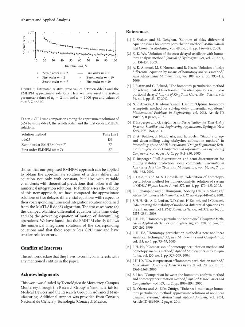