Research Article Application of Base Force Element …downloads.hindawi.com/journals/mpe/2015/292809.pdfResearch Article Application of Base Force Element Method on Complementary Energy

Research ArticleApplication of Base Force Element Method onComplementary Energy Principle to Rock Mechanics Problems

Yijiang Peng, Qing Guo, Zhaofeng Zhang, and Yanyan Shan

The Key Laboratory of Urban Security and Disaster Engineering, Ministry of Education, Beijing University of Technology,Beijing 100124, China

Correspondence should be addressed to Yijiang Peng; [email protected]

Received 24 August 2014; Accepted 5 September 2014

Academic Editor: Song Cen

Copyright © 2015 Yijiang Peng et al. This is an open access article distributed under the Creative Commons Attribution License,which permits unrestricted use, distribution, and reproduction in any medium, provided the original work is properly cited.

The four-mid-node plane model of base force element method (BFEM) on complementary energy principle is used to analyzethe rock mechanics problems. The method to simulate the crack propagation using the BFEM is proposed. And the calculationmethod of safety factor for rock mass stability was presented for the BFEM on complementary energy principle. The numericalresearches show that the results of the BFEM are consistent with the results of conventional quadrilateral isoparametric elementand quadrilateral reduced integration element, and the nonlinear BFEM has some advantages in dealing crack propagation andcalculating safety factor of stability.

1. Introduction

The finite element method (FEM) has been playing avery important role in solving various problems in engi-neering and science. However, the conventional finite ele-ment method (FEM) based on the displacement model hassome shortcomings, such as large deformation, treatment ofincompressible materials, bending of thin plates, and movingboundary problems. In the past decades, numerous effortstechniques have been proposed for developing finite elementmodels which are robust and insensitive to mesh distortion,such as the hybrid stress method [1–4], the equilibriummod-els [5, 6], themixed approach [7], the integrated forcemethod[8–11], the incompatible displacement modes [12, 13], theassumed strain method [14–17], the enhanced strain modes[18, 19], the selectively reduced integration scheme [20],the quasiconforming element method [21], the generalizedconforming method [22], the Alpha finite element method[23], the new spline finite element method [24, 25], theunsymmetric method [26–29], the new natural coordinatemethods [30–33], the smoothed finite element method [34],and the base force element method [35–43].

In recent years, some scholars are studying other typesof numerical analysis methods, such as boundary element

method [44, 45] and meshless method [46, 47]. And somescholars still adhere to explore the finite element methodbased on complementary energy principle [48–51]. However,these methods have not been widely applied in engineering.

In this paper, the base force element method (BFEM)on complementary energy principle is used to analyze theengineering problems of rock mechanics. The “base forces”was introduced by Gao [52], who used the concept to replacevarious stress tensors for the description of the stress stateat a point. These base forces can be directly obtained fromthe strain energy. For large deformation problems, when thebase forces were adopted, the derivation of basic formulaewas simplified by Gao [53] and Gao et al. [54–56]. Based onthe concept of the base forces, precise expressions for stiffnessand compliance matrices for the FEM were obtained by Gao[52]. The applications of the stiffness matrix to the planeproblems of elasticity using the plane quadrilateral elementand the polygonal element were researched by Peng et al.[37]. Using the concept of base forces as state variables, athree-dimensional formulation of base force elementmethod(BFEM) on complementary energy principle was proposedby Peng and Liu [35] for geometrically nonlinear problems.And the new finite element method based on the conceptof base forces was called as the Base Force Element Method

Hindawi Publishing CorporationMathematical Problems in EngineeringVolume 2015, Article ID 292809, 16 pageshttp://dx.doi.org/10.1155/2015/292809

2 Mathematical Problems in Engineering

I

J

K

L

Figure 1: Four-mid-node plane element.

(BFEM) by Peng and Liu [35]. A three-dimensional modelof base force element method (BFEM) on complementaryenergy principle was proposed by Liu and Peng [36] forelasticity problems. A 4-mid-node plane element model ofthe BFEM on complementary energy principle was proposedby Peng et al. [38] for geometrically nonlinear problem,which is derived by assuming that the stress is uniformlydistributed on each edges of a plane element. In the paper[39], an arbitrary convex polygonal element model of theBFEM on complementary energy principle was proposedfor geometrically nonlinear problem. In the paper [43], a 4-mid-node plane model of BFEM on complementary energyprinciple was researched, and its computational performancewas studied. The convex polygonal element model of BFEMon complementary energy principle was given by Peng et al.[40] for arbitrary mesh problems. In the paper [41], the con-cave polygonal element model of BFEM on complementaryenergy principle was proposed for the concave polygonalmesh problems. In the paper [42], the BFEM on potentialenergy principle was used to analyze recycled aggregate con-crete (RAC) on mesolevel, in which the model of BFEMwithtriangular element was derived, and the simulation results ofthe BFEM agree with the test results of recycled aggregateconcrete. In recently, the BFEM on damage mechanics hasbeen used to analyze the compressive strength, the size effectsof compressive strength, and fracture process of concreteat mesolevel, and the analysis method is the new way forinvestigating fracture mechanism and numerical simulationof mechanical properties for concrete.

The purpose of this paper is to survey the base forces ele-ment method on complementary energy principle for large-scale computing problems in rock engineering problems.

2. Model of the BFEM

2.1. Compliance Matrix. Consider a 4-mid-node plane ele-ment as shown in Figure 1; the compliance matrix of a baseforce element can be obtained as [43]

C𝐼𝐽=

1 + ]𝐸𝐴

(𝑟𝐼𝐽U −

]1 + ]

r𝐼⊗ r𝐽) , (𝐼, 𝐽 = 1, 2, 3, 4) (1)

in which 𝐸 is Young’s modulus, ] is Poisson’s ratio, 𝐴 is thearea of an element, U is the unit tensor, and 𝑟

𝐼𝐽is the dot

product of radius vectors r𝐼and r𝐽at points 𝐼 and 𝐽.

For a plane rectangular coordinate system, the radiusvectors r

𝐼and r𝐽of points 𝐼 and 𝐽 can be written as

r𝐼= 𝑥𝐼e𝑥+ 𝑦𝐼e𝑦, r

𝐽= 𝑥𝐽e𝑥+ 𝑦𝐽e𝑦 (2)

in which e𝑥, e𝑦are the unit vectors.

Further, the compliance matrix of an element can bereduced as follows:

C𝐼𝐽=

1 + ]𝐸𝐴

[(

1

1 + ]𝑥𝐼𝑥𝐽+ 𝑦𝐼𝑦𝐽) e𝑥⊗ e𝑥

−

]1 + ]

𝑥𝐼𝑦𝐽e𝑥⊗ e𝑦−

]1 + ]

𝑦𝐼𝑥𝐽e𝑦⊗ e𝑥

+(𝑥𝐼𝑥𝐽+

1

1 + V𝑦𝐼𝑦𝐽) e𝑦⊗ e𝑦] .

(3)

For a plane strain problem, it is necessary to replace 𝐸 by𝐸/(1 − ]2) and ] by ]/(1 − ]) in (1) and (3).

The characteristics of the BFEM on complementaryenergy principle are that the model does not introduce aninterpolating function and is not necessary to introduce theGauss integral for calculating the compliance coefficient at apoint.

2.2. Governing Equations. The total complementary energyof the elastic system which has 𝑛 elements can be written as

Π𝐶= ∑

𝑛

(𝑊

𝑒

𝐶− u𝐼⋅ T𝐼) , (4)

where 𝑊𝑒𝐶is the complementary energy of an element and

T𝐼 and u𝐼are the resultant force vectors and the given

displacement acting on the center node 𝐼of the edge 𝐼, respec-tively.

The equilibrium conditions can be released by theLagrange multiplier method, and a new complementaryenergy function for an element can be introduced as follows:

Π

𝑒

𝐶

∗(T,𝜆, 𝜆

𝜃) = Π

𝑒

𝐶(T) + 𝜆(

4

∑

𝐼=1

T𝐼) + 𝜆𝜃(T𝐼 × r

𝐼) , (5)

where 𝜆 = 𝜆𝑥e𝑥+ 𝜆𝑦e𝑦and 𝜆

𝜃are the Lagrange multipliers.

For the elastic system, the modified total complementaryenergy function of the elastic system which contains 𝑛

elements should meet the following equation by means of themodified complementary energy principle:

𝛿Π∗

𝐶= ∑

𝑛

[𝛿Π𝑒

𝐶

∗(T,𝜆, 𝜆

𝜃)] = 0. (6)

Further, (6) can be expressed as

𝜕Π

∗

𝐶(T,𝜆, 𝜆

𝜃)

𝜕T= 0,

𝜕Π

∗

𝐶(T,𝜆, 𝜆

𝜃)

𝜕𝜆= 0,

𝜕Π

∗

𝐶(T,𝜆, 𝜆

𝜃)

𝜕𝜆𝜃

= 0.

(7)

Thefirst of (7) is the compatibility equations and displace-ment boundary conditions for the elastic system. According

Mathematical Problems in Engineering 3

to this equation, the displacement boundary conditions inthis paper can be implemented in the BFEM. The second of(7) is the force equilibrium equation of each element. Thethird of (7) is the moment equilibrium equation of eachelement. These are the governing equations of the BFEM.From the equations, we can obtain the resultant forces actingon the center points of the edges of all elements.

2.3. Stress Tensor of an Element. Consider the 4-mid-nodeplane element as shown in Figure 1; the real stress 𝜎 of theelement can be replaced by the average stress 𝜎 if the elementis small enough. According to the definitions of Cauchy stresstensors, the stress expressions of an element can be obtainedas

𝜎 =1

𝐴

T𝐼 ⊗ r𝐼, (8)

where ⊗ is the dyadic symbol,T𝐼 and r𝐼are the resultant force

vectors acting on the center node 𝐼of the edge 𝐼 and the radiusvector of the node 𝐼, respectively, and the summation rule isimplied.

For a plane rectangular coordinate system, the forcevectors T𝐼of the node 𝐼 can be written as

T𝐼 = 𝑇

𝐼

𝑥e𝑥+ 𝑇

𝐼

𝑦e𝑦, (9)

where 𝑇𝐼𝑥and 𝑇

𝐼

𝑦are the components of the force vector T𝐼

along coordinates 𝑥 and 𝑦, respectively.Further, the stress tensors of an element can be reduced

as follows:

𝜎 =1

𝐴

4

∑

𝐼=1

[𝑇

𝐼

𝑥𝑥𝐼e𝑥⊗ e𝑥+ 𝑇

𝐼

𝑥𝑦𝐼e𝑥⊗ e𝑦

+ 𝑇

𝐼

𝑦𝑥𝐼e𝑦⊗ e𝑥+ 𝑇

𝐼

𝑦𝑦𝐼e𝑦⊗ e𝑦] .

(10)

2.4. Displacement Vector of Nodes. According to the gov-erning equation of an element of the BFEM, the explicitexpression of displacement can be obtained as

𝛿𝐼= C𝐼𝐽⋅ T𝐽 + 𝜆 + 𝜆

𝜃𝜀 ⋅ r𝐼, (11)

in which 𝜀 is the alternating tensor, 𝜆 and 𝜆𝜃are the Lagrange

multipliers [43], and 𝜀 and 𝜆 can be expressed as

𝜀 = e𝑥⊗ e𝑦− e𝑦⊗ e𝑥,

𝜆 = 𝜆𝑥e𝑥+ 𝜆𝑦e𝑦.

(12)

Further, the displacement vectors of an element can bereduced as follows [43]:

𝛿𝐼= (𝐶𝐼𝑥𝐽𝑥

𝑇

𝐽

𝑥+ 𝐶𝐼𝑥𝐽𝑦

𝑇

𝐽

𝑦+ 𝜆𝑥+ 𝜆𝜃𝑦𝐼) e𝑥

+ (𝐶𝐼𝑦𝐽𝑥

𝑇

𝐽

𝑥+ 𝐶𝐼𝑦𝐽𝑦

𝑇

𝐽

𝑦+ 𝜆𝑦− 𝜆𝜃𝑥𝐼) e𝑦.

(13)

4

3

1

2

x

y

o

Q4y = −

𝜌gAt

4

Q3y = −

𝜌gAt

4

Q1y = −

𝜌gAt

4

Q2y = −

𝜌gAt

4

Figure 2: Equivalent node loads of gravity in an element.

3. Simulation of Gravity and Material

In engineering problems, regardless of the dam, rock slope,or other structure of rock mass, the gravity of structureshould be considered in the numerical calculation. We didnot take into account the gravity problemwhenwe previouslyprepared the program of BFEM on complementary energyprinciple. In order to consider the gravity of structure, threeproblems must be solved, including the calculation problemof equivalent node loads in the BFEM on complementaryenergy principle, the problem of exerting gravity in thesoftware of the BFEM and the calculation problem of stresstensor in an element when the gravity is added.

3.1. Equivalent Node Loads of Gravity. For the BFEM oncomplementary energy principle, the equivalent node loadsof gravity in an element can be calculated according to theprinciple of virtual work, as shown in Figure 2, and theexpression can be given as

{𝑄}

𝑒= −

𝜌𝑔𝐴𝑡

4

[0 1 0 1 0 1 0 1]

𝑇 (14)

or

Q𝐼 = −

𝜌𝑔𝐴𝑡

4

e𝑦, (𝐼 = 1, 2, 3, 4) , (15)

where 𝑡 is the thickness of an element, 𝜌 is the density ofmaterial, and 𝑔 is acceleration of gravity.

3.2. Stress Calculation of an Element. When the gravity of anelement is not taken into account, as shown in Figure 3, wecalculate the force acting on the edges of an element first.Then, the stress tensor of the element can be calculated by(8) or (10).

Further, the stress tensors of an element can also bereduced as follows:

𝜎 =1

𝐴

(T1 ⊗ r1+ T2 ⊗ r

2+ T3 ⊗ r

3+ T4 ⊗ r

4) , (16)

where T𝐼 = 𝑇

𝐼

𝑥e𝑥+ 𝑇

𝐼

𝑦e𝑦, r𝐼 = 𝑥

𝐼e𝑥+ 𝑦𝐼e𝑦, (𝐼 = 1, 2, 3, 4), 𝑥

𝐼

and 𝑦𝐼are the coordinates of node 𝐼, respectively.


4

3

1

2

x

y

o

T4y

T3y

T1y

T4x

T3x T2

y

T2x

T1x

Figure 3: An element without gravity.

4

3

1

2

x

y

o

T4x

T3x

T1x

A free boundary

T4y + Q4

y

T3y + Q3

y

T1y + Q1

y

Q2y

Figure 4: Considering gravity and a free boundary.

When the gravity of an element is taken into account andthere is a free boundary, as shown in Figure 4, the stress tensorof the element can be calculated as

𝜎 =1

𝐴

[(T1 +Q1) ⊗ r1+Q2 ⊗ r

2

+ (T3 +Q3) ⊗ r3+ (T4 +Q4) ⊗ r

4] .

(17)

When the gravity of an element is taken into account andthere is a force boundary condition, as shown in Figure 5, thestress tensor of the element can be calculated as

𝜎 =1

𝐴

[(T1 +Q1) ⊗ r1+ (F +Q2) ⊗ r

2

+ (T3 +Q3) ⊗ r3+ (T4 +Q4) ⊗ r

4]

(18)

in which F = 𝐹𝑥e𝑥+ 𝐹𝑦e𝑦.

When the gravity of an element is not taken into accountand there is a force boundary condition, as shown in Figure 6,the stress tensor of the element can be calculated as

𝜎 =1

𝐴

(T1 ⊗ r1+ F ⊗ r

2+ T3 ⊗ r

3+ T4 ⊗ r

4) . (19)

3.3. Simulation of Different Materials. We adopt two one-dimensional array variables to reflect the change of elasticmodulus and Poisson’s ratio of different materials, respec-tively.

4

3

1

2

x

y

o

T4x

T3x

T1x

Fx

A force boundary condition

T4y + Q4

y

T3y + Q3

y

T1y + Q1

y

Fy + Q2y

Figure 5: Considering gravity and a force boundary condition.

4

3

1

2

A force boundary condition

x

y

o

T4y

T3y

T1y

T4x

T3x

T1x

Fy

Fx

Figure 6: Considering a force boundary condition and no gravity.

4. The Nonlinear Model of BFEM for CrackPropagation Problems

The conventional displacement model of FEM requires themesh reconstruction for the crack propagation problems.Therefore, the conventional FEM has deficiencies for thecrack propagation problems. Because the contact forcesbetween each element are used, the BFEMon complementaryenergy principle has advantage in the simulation of crackpropagation problems. In the BFEM on complementaryenergy principle, we only need to deal with the constraintconditions and compatibility equations of displacement.

4.1. Failure Criteria of the Contact Interface between TwoElements. According to the control equations of the BFEMon complementary energy principle, the forces acting on theedge on an element can easily be calculated. According to thefailure criteria expressed by the forces acting on the edge ofan element, we can judge whether the interface of elementsis cracking. If there is cracking of element interface, thenonlinear processing must be carried out.

4.1.1. Condition of Elastic State at Contact Interface. When𝑇𝑛< 0 and |𝑇

𝑠| < −𝑓 ⋅ 𝑇

𝑛+ 𝑐 ⋅ 𝑙 or 0 < 𝑇

𝑛< 𝑡0and |𝑇

𝑠| < 𝑐 ⋅ 𝑙,

the contact interface is not cracked and in the elastic state.Here, 𝑇

𝑛and 𝑇

𝑠are the normal interface force and tangential

interface force at contact interface between two elements,


respectively. 𝑐 and𝑓 are the cohesion and the internal frictioncoefficient of the contact interface, respectively. 𝑙 is the lengthof an element. 𝑡

0is the tensile strength of an element, and it

is positive in tension.

4.1.2. Condition of Positive Slip at Contact Interface. When𝑇𝑛< 0 and 𝑇

𝑠≥ −𝑓 ⋅ 𝑇

𝑛+ 𝑐 ⋅ 𝑙, the contact interface of the two

elements began to slip. We need to get rid of the tangentialdisplacement constraint at the contact interface between thetwo elements that it has been cracked and put the frictionalforce as load that is used to an initial force condition.The newload acting on the contact interface between the two elementsin the second loop of calculation can be written as follows:

𝑇𝑠0= 𝑓 ⋅ 𝑇

𝑠. (20)

When 0 < 𝑇𝑛

< 𝑡0and 𝑇

𝑠≥ 𝑐 ⋅ 𝑙, the contact

interface of the two elements begins to slip. We need to getrid of the tangential displacement constraint and the normaldisplacement constraint at the contact interface of the twoelements. And the contact interface will crack after slipping.

4.1.3. Condition of Negative Slip at Contact Interface. When𝑇𝑛< 0 and 𝑇

𝑠≤ 𝑓 ⋅ 𝑇

𝑛− 𝑐 ⋅ 𝑙, the contact interface of the two

elements began to slip. We need to get rid of the tangentialdisplacement constraint at the contact interface between thetwo elements that it has been cracked, and put the frictionalforce as load that is an initial force condition. The new loadacting on the contact interface between the two elements inthe second loop of calculation is

𝑇𝑠0= −𝑓 ⋅ 𝑇

𝑠. (21)

When 0 < 𝑇𝑛

< 𝑡0and 𝑇

𝑠≤ −𝑐 ⋅ 𝑙, the contact

interface of the two elements begins to slip. We need to getrid of the tangential displacement constraint and the normaldisplacement constraint at the contact interfaces of elements.And the contact interface will crack after slipping.

4.1.4. Condition of Pull Cracking at Contact Interface. When𝑇𝑛≥ 𝑡0, the contact interface of the two elements begins

to crack. We need to get rid of the tangential displacementconstraint and the normal displacement constraint at thecontact interfaces of elements.

After the above checks, the computer program of BFEMuses the new loads and constraint conditions to solve thegoverning equations of BFEM on complementary energyprinciple and obtains the new forces acting on the contactinterfaces of elements.The program repeats the above checksuntil there are no new cracking at the contact interfaces or thesolutions of nonlinear equations cannot be convergence sincethe interface cracks are too long.

4.2. Flow Chart of the Nonlinear BEFM for Crack PropagationProblems. The flow chart of the nonlinear BEFM of crackpropagation problems can be shown in Figure 7.

Start

Input information of elements, nodes, and materials

Input information of loads and boundary

Calculate indication array on degree of freedom for structure

Calculate compliance matrix of elements

Generate coefficient matrix and free term array of governing equations

Finish

Solve equations and get the forces acting on the surfaces of elements

Calculate displacements of nodes and stresses of elements

Output results

Use failure criteria to checkthe interface cracking

No

Yes

Figure 7: Flow chart of the nonlinear BEFM for crack propagationproblems.

10m

5m

𝜌

Figure 8: A rock pillar under the action of gravity.

5. Calculation Method on Safety Factor ofStability in the BFEM

There are many methods to calculate the safety factor inengineering. The traditional finite element method usuallyused the rock joint elements to calculate factor of safetyalong the joint path. When the base force element method


(a) 100 elements, 220 nodes (b) 200 elements, 430 nodes (c) 300 elements, 640 nodes

Figure 9: Three kinds of meshes for a rock pillar.

is used to analyze the stability of the rock mass in order toget the safety factor along the joint path, it is very easy. First,we calculate the surface forces of all elements according tothe different load combinations. Then, we accumulate thesliding resistances and the sliding forces along the slidingpath, respectively. Further, the safety factor of stability alongthe sliding path can obtained by the following equation:

𝐾 =

∑

𝑛

𝑖=1(−𝑇𝑛𝑖𝑓𝑖+ 𝑐𝑖𝑙𝑖)

∑

𝑛

𝑖=1𝑇𝑠𝑖

, (22)

where𝑇𝑛𝑖and𝑇𝑠𝑖are the normal interface force and tangential

interface force at contact interface between two elementsalong the sliding path, respectively. 𝑐

𝑖and 𝑓𝑖are the cohesion

and the internal friction coefficient of the contact interfacebetween two elements along the sliding path, respectively. 𝑙

𝑖

is the length of the interface in the element along the slidingpath.

6. Numerical Examples

6.1. Example 1: A Rock Pillar under the Action of Gravity.Consider a thick pillar of rock under the action of gravityshown in Figure 8. And its width is 5m, its height is 10m,modulus of elasticity 𝐸 = 1 × 10

8 Pa, Poisson ratio ] = 0.3,density of rock 𝜌 = 2.45 t/m3, and acceleration of gravity𝑔 = 9.8m/s2. The calculation is considered into the planestress problem.

The calculation is done using three different elementmeshes with the center nodes of edges of elements as shownin Figure 9.

The values of stress components and displacement com-ponents of the rock pillar are listed in Tables 1–4, respectively.Comparisons of the results from the conventional quadri-lateral isoparametric element (Q4 model) and quadrilateralreduced integration element (Q4R model) are also given inTables 1–4, respectively. The numerical results of the present

Table 1: Displacement 𝑢𝑦at the top of the pillar.

Meshes BFEMmodel(×10−2m)

Q4 model(×10−2m)

Q4R model(×10−2m)

10 × 10 −1.1939 −1.1917 −1.204810 × 20 −1.1940 −1.1931 −1.196410 × 30 −1.1940 −1.1934 −1.1940

Table 2: Displacement 𝑢𝑦at ℎ = 5m of the pillar.

Meshes BFEM(×10−3m)

Q4 model(×10−3m)


10 × 10 −8.7592 −8.6975 −8.804510 × 20 −8.7630 −8.7118 −8.672610 × 30 −8.7637 −8.7149 −8.7363

Table 3: Stress 𝜎𝑥at center of the elements at top of the pillar.

Meshes BFEM (kPa) Q4 model(kPa)

Q4R model(kPa)

10 × 10 −12.016 −12.244 −12.06210 × 20 −6.005 −6.0773 −6.01310 × 30 −4.003 −4.0382 −4.002

Table 4: Stress 𝜎𝑦at center of the elements at bottom of the pillar.


Q4R model(kPa)

10 × 10 −244.194 −242.945 −244.34910 × 20 −262.976 −260.116 −263.38710 × 30 −272.102 −268.002 −272.552

model are consistent with those of the Q4 model and Q4Rmodel and have shown good computational stability.


1

2

3

4

𝜏 = 1𝜏 = 1

𝜏 = 1

Figure 10: A rock pillar with four kinds of materials.

Figure 11: Mesh with 200 elements, 430 nodes.

Table 5: Stress solution of the pillar with four kinds of materialsunder uniform shearing forces.

𝜎𝑥

𝜏𝑥𝑦

𝜎𝑦

BFEM 0.000 1.000 0.000Exact 0.000 1.000 0.000

6.2. Example 2: Analysis for a Rock Pillar with Four Materialsunder Pure Shear Effect. Consider a rock pillar with fourmaterials under pure shear effect shown in Figure 10. Andits modulus of elasticity 𝐸

1= 10

9, 𝐸2= 10

8, 𝐸3= 10

7,and 𝐸

4= 10

6, respectively. And Poisson ratio ] = 0.3,the shear stress on surface of the structure 𝜏 = 1. Thecalculation is considered into the plane stress problem andthe dimensionless values.

The calculation is done using the mesh with the centernodes of edges of elements as shown in Figure 11.

The values of stress components of the rock pillar arelisted inTable 5, respectively. Comparisons of the results fromthe theoretical analysis are also given in Table 5, respectively.

10m

5m

Figure 12: A rock pillar subjected to water pressure and gravity.

Table 6: Displacement 𝑢𝑥at 𝑥 = 2.5m of the pillar top.


Q4 model(×10−2m)


20 × 40 4.0219 4.0056 4.019010 × 40 4.0415 4.0094 4.03988 × 40 4.0563 4.0135 4.05326 × 40 4.0891 4.0239 4.0863

Table 7: Displacement 𝑢𝑥at ℎ = 5m on the right of the pillar.


Q4 model(×10−2m)


20 × 40 2.0837 2.0758 2.083010 × 40 2.0816 2.0667 2.08158 × 40 2.0820 2.0626 2.08236 × 40 2.0849 2.0566 2.0862

Thenumerical results of the presentmodel are consistentwiththose of the theoretical analysis.

6.3. Example 3: A Rock Pillar under Water Pressure andGravity. Consider a rock pillar under water pressure andgravity shown in Figure 12. And its modulus of elasticity 𝐸 =

10

8 Pa, Poisson’ ratio ] = 0.3, density of rock 𝜌1= 2.4 t/m3,

density of water 𝜌2= 1.0 t/m3, and acceleration of gravity

𝑔 = 9.8m/s2. The calculation is considered into the planestrain problem.

The calculation is done using four different elementmeshes with the center nodes of edges of elements as shownin Figure 13.

The values of stress components and displacement com-ponents of the rock pillar are listed in Tables 6–12, respec-tively. Comparisons of the results from the conventionalquadrilateral isoparametric element (Q4 model) and quadri-lateral reduced integration element (Q4R model) are alsogiven in Tables 6–12, respectively. The numerical results ofthe present model are consistent with those of Q4R model,


(a) 800 elements, 1660nodes

(b) 400 elements, 850nodes

(c) 320 elements, 688nodes

(d) 240 elements, 526nodes

Figure 13: Four kinds of meshes for a rock pillar.

Table 8: Displacement 𝑢𝑦at 𝑥 = 2.5m of the pillar top.


Q4 model(×10−3m)


20 × 40 −9.8891 −9.8869 −9.889510 × 40 −9.8888 −9.8856 −9.88988 × 40 −9.8889 −9.8850 −9.89436 × 40 −9.8889 −9.8840 −9.8926

Table 9: Displacement 𝑢𝑦at ℎ = 5m on the right of the pillar.

Meshes BFEMmodel(×10−2m)

Q4 model(×10−2m)


20 × 40 −1.5918 −1.5878 −1.591310 × 40 −1.5488 −1.5412 −1.54838 × 40 −1.5290 −1.51894 −1.52846 × 40 −1.4983 −1.4832 −1.4975

Table 10: Stress 𝜎𝑥at center of the element at lower right of pillar.


Q4R model(kPa)

20 × 40 −128.963 −179.706 −132.97410 × 40 −142.729 −191.962 −150.8398 × 40 −141.996 −193.919 −152.8156 × 40 −134.954 −194.249 −150.941

and the 4-mid-node element of BFEM has given goodperformance compared with Q4 model for the large aspectratio of elements. Due to the different method calculatingthe equivalent node loads of water pressure between the baseforce elements and the element of traditional FEM, there isa slight error about the calculation results of the horizontalstresses 𝜎

𝑥of the element in lower right corner of rock pillar

between the BFEM and the Q4Rmodel, as shown in Table 10.

Table 11: Stress 𝜏𝑥𝑦

at center of the element at lower right of pillar.


Q4R model(kPa)

20 × 40 152.442 172.480 153.36610 × 40 153.439 167.708 154.6378 × 40 151.262 163.966 152.6126 × 40 146.664 157.624 148.288

Table 12: Stress 𝜎𝑦at center of the element at lower right of pillar.


Q4R model(kPa)

20 × 40 −802.328 −796.173 −802.74110 × 40 −707.932 −700.016 −708.5828 × 40 −675.867 −666.975 −676.6166 × 40 −634.179 −623.753 −635.039

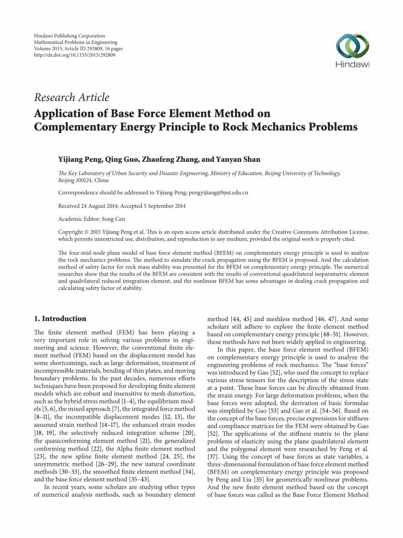
6.4. Example 4: Stress Analysis of Concrete Gravity Dam.Consider a concrete gravity dam shown in Figure 14. Andheight of the dam is 65m, bottom width is 49m, the waterlevel is 60m, the elastic modulus of concrete 𝐸

1= 15GPa,

Poisson ratio of concrete ]1

= 0.2, the elastic modulusof rock 𝐸

2= 30GPa, Poisson ratio of rock ]

2= 0.3,

density of concrete is 2.45 t/m3, density of water is 1 t/m3,and acceleration of gravity 𝑔 = 9.8m/s2. The calculation isconsidered into the plane strain problem and considered theeffect of rock foundation of the dam.

The calculation is done using the mesh with the centernodes of edges of elements as shown in Figure 15. In thiscalculation, we do not consider the initial geostress field. Theboundaries of the foundation are used the fixed constraint.The origin of coordinates is located at the bottom of the dam,and is 25 meters away from the dam heel.


15

65

49

1 : 0.7

Figure 14: A concrete gravity dam.

Figure 15: Meshes of the dam and its foundation (1344 elements,2809 nodes).

BFEMQ4 modelQ4R model

10 20 30 40 50 60

h (m)

0.0

−0.1

−0.2

−0.3

−0.6

−0.5

−0.4

𝜎x

(MPa

)

Figure 16: The ℎ-𝜎𝑥curves at the upstream face of the dam.


10 20 30 40 50 60

h (m)

−0.10

−0.05

0.00

0.05

0.10

0.15

𝜏xy

(MPa

)

Figure 17: The ℎ-𝜏𝑥𝑦

curves at the upstream face of the dam.


0 10 20 30 40 50 60

h (m)

0.0

−0.2

−0.4

−0.6

−1.0

−0.8

𝜎y

(MPa

)

Figure 18: The ℎ-𝜎𝑦curves at the upstream face of the dam.

The values of stress components and displacement com-ponents of the dam are plotted in Figures 16–25, respectively.Comparisons of the results from the conventional quadri-lateral isoparametric element (Q4 model) and quadrilateralreduced integration element (Q4R model) are also givenin Figures 16–25, respectively. The numerical results of thepresent model are consistent with those of the Q4 model andQ4R model and have shown good computational stability.

6.5. Example 5: Simulation and Analysis on the HorizontalCrack Propagation of Rock Block. Consider a rock block sub-jected by the horizontal thrust and vertical pressure shown inFigure 26. For the convenience of study, we do not considerthe weight. Andwe use the dimensionless numerical analysis.



0 10 20 30 40 50 60

h (m)

1.0

1.5

2.0

2.5

3.0

ux

(mm

)

Figure 19: The ℎ-𝑢𝑥curves at the upstream face of the dam.


−1.0

−1.5

−2.0

−2.5

−3.0

−3.5

−4.0

uy

(mm

)

0 10 20 30 40 50 60

h (m)

Figure 20: The ℎ-𝑢𝑦curves at the upstream face of the dam.

Assuming elasticmodulus𝐸 = 1, Poisson ratio ] = 0.3, tensilestrength of a large number, and the uniform load 𝑝

1= 1

and 𝑝2= 1. The calculation is considered into the plane

stress problem and the dimensionless values.The calculation is done using the mesh with the center

nodes of edges of elements as shown in Figure 27.In order to check whether the interface between the rock

block and the ground will crack, we assume the frictioncoefficient of interface 𝑓 = 0.5 and change the value ofinterface cohesion 𝑐.The results of calculation using the com-puter program of the nonlinear BFEM shown in Section 4and the failure criteria in Section 4.1 are as follows.

(1) When 𝑐 = 10, there is no cracks.(2) When 𝑐 = 2.8, there is one element interface crack.


−25 −20 −15 −10 −5 0

x (m)

0.0

−0.1

−0.2

−0.3

−0.5

−0.4

𝜎x

(MPa

)

Figure 21: The ℎ-𝜎𝑥curves at the half height of the dam.


−25 −20 −15 −10 −5 0

x (m)

−0.4

−0.5

−0.6

−0.7

−0.8𝜎y

(MPa

)

Figure 22: The ℎ-𝜎𝑦curves at the half height of the dam.

(3) When 𝑐 = 2, there are three elements’ interfacescracks.

(4) When 𝑐 = 1.5, there are five elements’ interfacescracks.

(5) When 𝑐 = 1.1, there are seven elements’ interfacescracks.

(6) When 𝑐 = 1.0, the cracks are too long, and too littlestructural constraints have been insufficient to solvethe equations.

When the interface cohesion 𝑐 is 1.5, the case of crackpropagation of rock block is shown in Figure 28, and thesafety factor of stability is 𝐾 = 2 which is consistent with



−25 −20 −15 −10 −5 0

x (m)

0.00

0.05

0.10

0.15

0.20

0.25

0.30

𝜏xy

(MPa

)

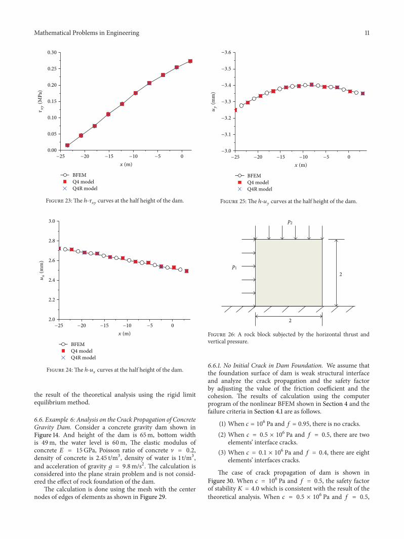
Figure 23: The ℎ-𝜏𝑥𝑦

curves at the half height of the dam.


2.0

2.2

2.4

2.6

2.8

3.0

ux

(mm

)

−25 −20 −15 −10 −5 0

x (m)

Figure 24: The ℎ-𝑢𝑥curves at the half height of the dam.

the result of the theoretical analysis using the rigid limitequilibrium method.

6.6. Example 6: Analysis on the Crack Propagation of ConcreteGravity Dam. Consider a concrete gravity dam shown inFigure 14. And height of the dam is 65m, bottom widthis 49m, the water level is 60m, The elastic modulus ofconcrete 𝐸 = 15GPa, Poisson ratio of concrete ] = 0.2,density of concrete is 2.45 t/m3, density of water is 1 t/m3,and acceleration of gravity 𝑔 = 9.8m/s2. The calculation isconsidered into the plane strain problem and is not consid-ered the effect of rock foundation of the dam.

The calculation is done using the mesh with the centernodes of edges of elements as shown in Figure 29.


−25 −20 −15 −10 −5 0

x (m)

−3.0

−3.1

−3.2

−3.3

−3.4

−3.5

−3.6

uy

(mm

)

Figure 25: The ℎ-𝑢𝑦curves at the half height of the dam.

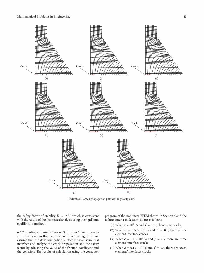
2

2

p1

p2

Figure 26: A rock block subjected by the horizontal thrust andvertical pressure.

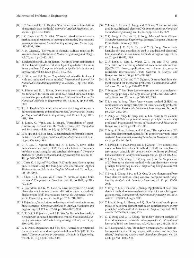
6.6.1. No Initial Crack in Dam Foundation. We assume thatthe foundation surface of dam is weak structural interfaceand analyze the crack propagation and the safety factorby adjusting the value of the friction coefficient and thecohesion. The results of calculation using the computerprogram of the nonlinear BFEM shown in Section 4 and thefailure criteria in Section 4.1 are as follows.

(1) When 𝑐 = 10

6 Pa and 𝑓 = 0.95, there is no cracks.(2) When 𝑐 = 0.5 × 10

6 Pa and 𝑓 = 0.5, there are twoelements’ interface cracks.

(3) When 𝑐 = 0.1 × 10

6 Pa and 𝑓 = 0.4, there are eightelements’ interfaces cracks.

The case of crack propagation of dam is shown inFigure 30. When 𝑐 = 10

6 Pa and 𝑓 = 0.5, the safety factorof stability 𝐾 = 4.0 which is consistent with the result of thetheoretical analysis. When 𝑐 = 0.5 × 10

6 Pa and 𝑓 = 0.5,


Figure 27: Meshes of the rock block.

Crack

(a) In the first cycle calculation

Crack

(b) In the second cycle calculation

Crack

(c) In the third cycle calculation

Crack

(d) In the fourth cycle calculation

Crack

(e) In the fifth cycle calculation

Figure 28: Crack propagation path of the rock block.

Figure 29: Mesh of gravity dam (800 elements, 1660 nodes).


Crack

(a)

Crack

(b)

Crack

(c)

Crack

(d)

Crack

(e)

Crack

(f)

Crack

(g)

Crack

(h)

Figure 30: Crack propagation path of the gravity dam.

the safety factor of stability 𝐾 = 2.55 which is consistentwith the results of the theoretical analysis using the rigid limitequilibrium method.

6.6.2. Existing an Initial Crack in Dam Foundation. There isan initial crack in the dam heel as shown in Figure 31. Weassume that the dam foundation surface is weak structuralinterface and analyze the crack propagation and the safetyfactor by adjusting the value of the friction coefficient andthe cohesion. The results of calculation using the computer

program of the nonlinear BFEM shown in Section 4 and thefailure criteria in Section 4.1 are as follows.

(1) When 𝑐 = 10

6 Pa and 𝑓 = 0.95, there is no cracks.(2) When 𝑐 = 0.5 × 10

6 Pa and 𝑓 = 0.5, there is oneelement interface cracks.

(3) When 𝑐 = 0.1 × 10

6 Pa and 𝑓 = 0.5, there are threeelement’ interface cracks.

(4) When 𝑐 = 0.1 × 10

6 Pa and 𝑓 = 0.4, there are sevenelements’ interfaces cracks.


Figure 31: A gravity dam with a crack at the dam heel.

7. Conclusions

In this paper, the base force element method (BFEM) oncomplementary energy principle is used to analyze the rockmechanics problems. The methods to simulate the gravity ofan element, the crack propagation and the safety factor of sta-bility are proposed for the BFEM on complementary energyprinciple. The following conclusions can be drawn.

(1) The calculation results of the BFEM on complemen-tary energy principle show that the numerical resultsof the present method coincide with the theoreticalsolution, the results of conventional quadrilateralisoparametric element (Q4 model) and quadrilat-eral reduced integration element (Q4R model). Thecorrectness of the present method and its computerprogram is verified.

(2) The research results show that the BFEM on comple-mentary energy principle has a good computationalprecision and stability is not sensitive to the effects onthe aspect ratio of element and can be used for large-scale scientific and engineering computing.

(3) The results of the BFEM for crack propagation prob-lems show that the nonlinear BFEM can solve thecracking problem and simulate the crack propagationof the interface in rock mechanics engineering.

(4) The BFEM on complementary energy principle wasapplied to analyze the stability of rock mass and dam,and the results of safety factor are consistent with theresults of the theoretical solutions using the rigid limitequilibrium method. The research results show thepresent method can be easily used to calculate thesafety factor in rock engineering.

(5) This paper researched only the cracking problemswith horizontal crack in rock mass and calculatedonly the safety factor of a single slip channel in rockmass.

(6) The cracking problems of inclined cracks and thesafety factor of multiple sliding channels in rock massare studying, and the further research results will bepublished in the future.

Conflict of Interests

The authors declare that there is no conflict of interests.

Acknowledgments

This work is supported by the National Natural ScienceFoundation of China, nos. 10972015 and 11172015 and thepreexploration project of the Key Laboratory of Urban Secu-rity and Disaster Engineering, Ministry of Education, BeijingUniversity of Technology, no. USDE201404.

References

[1] T. H. H. Pian, “Derivation of element stiffness matrices byassumed stress distributions,” AIAA Journal, vol. 2, no. 7, pp.1333–1336, 1964.

[2] T. H. Pian and D. P. Chen, “Alternative ways for formulationof hybrid stress elements,” International Journal for NumericalMethods in Engineering, vol. 18, no. 11, pp. 1679–1684, 1982.

[3] T. H. H. Pian and K. Sumihara, “Rational approach for assumedstress finite elements,” International Journal for NumericalMethods in Engineering, vol. 20, no. 9, pp. 1685–1695, 1984.

[4] C. Zhang, D. Wang, J. Zhang, W. Feng, and Q. Huang, “On theequivalence of various hybrid finite elements and a new orthog-onalization method for explicit element stiffness formulation,”Finite Elements in Analysis and Design, vol. 43, no. 4, pp. 321–332, 2007.

[5] B. Fraeijs de Veubeke, “Displacement and equilibrium mod-els in the finite element method,” in Stress Analysis, O. C.Zienkiewicz and G. S. Holister, Eds., pp. 145–197, John Wiley &Sons, New York, NY, USA, 1965.

[6] B. F. de Veubeke, “A new variational principle for finite elasticdisplacements,” International Journal of Engineering Science, vol.10, no. 9, pp. 745–763, 1972.

[7] R. L. Taylor and O. C. Zienkiewicz, “Complementary energywith penalty functions in finite element analysis,” in EnergyMethods in Finite Element Analysis, R. Glowinski, Ed., pp. 153–174, John Wiley & Sons, New York, NY, USA, 1979.

[8] S. N. Patniak, “An integrated forcemethod for discrete analysis,”International Journal for Numerical Methods in Engineering, vol.6, no. 2, pp. 237–251, 1973.

[9] S. N. Patnaik, “The integrated force method versus the standardforce method,” Computers and Structures, vol. 22, no. 2, pp. 151–163, 1986.

[10] S. N. Patnaik, “The variational energy formulation for theintegrated force method,” AIAA Journal, vol. 24, no. 1, pp. 129–137, 1986.

[11] S. N. Patnaik, L. Berke, and R. H. Gallagher, “Integratedforce method versus displacement method for finite elementanalysis,” Computers and Structures, vol. 38, no. 4, pp. 377–407,1991.

[12] E. L. Wilson, R. L. Tayler, W. P. Doherty, and J. Ghaboussi,“Incompatible displacement models,” in Numerical and Com-putational Methods in Structural Mechanics, S. J. Fenves, N.Perrone, A. R. Robinson, and W. C. Schnobrich, Eds., pp. 43–57, Academic Press, New York, NY, USA, 1973.

[13] R. L. Taylor, P. J. Beresford, and E. L. Wilson, “A non-conforming element for stress analysis,” International Journalfor Numerical Methods in Engineering, vol. 10, no. 6, pp. 1211–1219, 1976.


[14] J. C. Simo and T. J. R. Hughes, “On the variational foundationsof assumed strain methods,” Journal of Applied Mechanics, vol.53, no. 1, pp. 51–54, 1986.

[15] J. C. Simo and M. S. Rifai, “Class of mixed assumed strainmethods and themethod of incompatible modes,” InternationalJournal for Numerical Methods in Engineering, vol. 29, no. 8, pp.1595–1638, 1990.

[16] R. H. Macneal, “Derivation of element stiffness matrices byassumed strain distributions,” Nuclear Engineering and Design,vol. 70, no. 1, pp. 3–12, 1982.

[17] T. Belytschko and L. P. Bindeman, “Assumed strain stabilizationof the 4-node quadrilateral with 1-point quadrature for non-linear problems,” Computer Methods in Applied Mechanics andEngineering, vol. 88, no. 3, pp. 311–340, 1991.

[18] R. Piltner and R. L. Taylor, “A quadrilateral mixed finite elementwith two enhanced strain modes,” International Journal forNumerical Methods in Engineering, vol. 38, no. 11, pp. 1783–1808,1995.

[19] R. Piltner and R. L. Taylor, “A systematic constructions of B-bar functions for linear and nonlinear mixed-enhanced finiteelements for plane elasticity problems,” International Journal forNumerical Methods in Engineering, vol. 44, no. 5, pp. 615–639,1997.

[20] T. J. R. Hughes, “Generalization of selective integration proce-dures to anisotropic andnonlinearmedia,” International Journalfor Numerical Methods in Engineering, vol. 15, no. 9, pp. 1413–1418, 1980.

[21] T. Limin, C. Wanji, and L. Yingxi, “Formulation of quasi-conforming element and Hu-Washizu principle,” Computersand Structures, vol. 19, no. 1-2, pp. 247–250, 1984.

[22] L. Yu-qiu andH.Min-feng, “A generalized conforming isopara-metric element,”AppliedMathematics andMechanics, vol. 9, no.10, pp. 929–936, 1988.

[23] G. R. Liu, T. Nguyen-Thoi, and K. Y. Lam, “A novel alphafinite element method (𝛼FEM) for exact solution to mechanicsproblems using triangular and tetrahedral elements,” ComputerMethods in Applied Mechanics and Engineering, vol. 197, no. 45–48, pp. 3883–3897, 2008.

[24] J. Chen, C.-J. Li, andW.-J. Chen, “A 17-node quadrilateral splinefinite element using the triangular area coordinates,” AppliedMathematics and Mechanics (English Edition), vol. 31, no. 1, pp.125–134, 2010.

[25] J. Chen, C.-J. Li, and W.-J. Chen, “A family of spline finiteelements,” Computers and Structures, vol. 88, no. 11-12, pp. 718–727, 2010.

[26] S. Rajendran and K. M. Liew, “A novel unsymmetric 8-nodeplane element immune to mesh distortion under a quadraticdisplacement field,” International Journal for Numerical Meth-ods in Engineering, vol. 58, no. 11, pp. 1713–1748, 2003.

[27] S. Rajendran, “A technique to developmesh-distortion immunefinite elements,” Computer Methods in Applied Mechanics andEngineering, vol. 199, no. 17–20, pp. 1044–1063, 2010.

[28] E. T. Ooi, S. Rajendran, and J. H. Yeo, “A 20-node hexahedronelementwith enhanced distortion tolerance,” International Jour-nal for Numerical Methods in Engineering, vol. 60, no. 15, pp.2501–2530, 2004.

[29] E. T. Ooi, S. Rajendran, and J. H. Yeo, “Remedies to rotationalframe dependence and interpolation failure of US-QUAD8 ele-ment,” Communications in Numerical Methods in Engineering,vol. 24, no. 11, pp. 1203–1217, 2008.

[30] Y. Long, L. Juxuan, Z. Long, and C. Song, “Area co-ordinatesused in quadrilateral elements,” Communications in NumericalMethods in Engineering, vol. 15, no. 8, pp. 533–543, 1999.

[31] Y. Q. Long, S. Cen, and Z. F. Long, Advanced Finite ElementMethod in Structural Engineering, Springer/TsinghuaUniversityPress, Berlin, Germany, 2009.

[32] Z. F. Long, J. X. Li, S. Cen, and Y. Q. Long, “Some basicformulae for area coordinates used in quadrilateral elements,”Communications in Numerical Methods in Engineering, vol. 15,no. 12, pp. 841–852, 1999.

[33] Z.-F. Long, S. Cen, L. Wang, X.-R. Fu, and Y.-Q. Long,“The third form of the quadrilateral area coordinate method(QACM-III): theory, application, and scheme of compositecoordinate interpolation,” Finite Elements in Analysis andDesign, vol. 46, no. 10, pp. 805–818, 2010.

[34] G. R. Liu, K. Y. Dai, and T. T. Nguyen, “A smoothed finite ele-ment method for mechanics problems,” Computational Mech-anics, vol. 39, no. 6, pp. 859–877, 2007.

[35] Y. Peng and Y. Liu, “Base force element method of complemen-tary energy principle for large rotation problems,” Acta Mech-anica Sinica, vol. 25, no. 4, pp. 507–515, 2009.

[36] Y. Liu and Y. Peng, “Base force element method (BFEM) oncomplementary energy principle for linear elasticity problem,”Science China: Physics, Mechanics and Astronomy, vol. 54, no. 11,pp. 2025–2032, 2011.

[37] Y. Peng, Z. Dong, B. Peng, and Y. Liu, “Base force elementmethod (BFEM) on potential energy principle for elasticityproblems,” International Journal of Mechanics and Materials inDesign, vol. 7, no. 3, pp. 245–251, 2011.

[38] Y. Peng, Z. Dong, B. Peng, and N. Zong, “The application of 2Dbase force elementmethod (BFEM) to geometrically non-linearanalysis,” International Journal of Non-LinearMechanics, vol. 47,no. 3, pp. 153–161, 2012.

[39] Y.-J. Peng, J.-W. Pu, B. Peng, and L.-J. Zhang, “Two-dimensionalmodel of base force element method (BFEM) on complemen-tary energy principle for geometrically nonlinear problems,”Finite Elements in Analysis and Design, vol. 75, pp. 78–84, 2013.

[40] Y. J. Peng, N. N. Zong, L. J. Zhang, and J. W. Pu, “Applicationof 2D base force element method with complementary energyprinciple for arbitrary meshes,” Engineering Computations, vol.31, no. 4, pp. 1–15, 2014.

[41] Y. Peng, L. Zhang, J. Pu, and Q. Guo, “A two-dimensional baseforce element method using concave polygonal mesh,” Eng-ineering Analysis with Boundary Elements, vol. 42, pp. 45–50,2014.

[42] Y. Peng, Y. Liu, J. Pu, and L. Zhang, “Application of base forceelement method to mesomechanics analysis for recycled aggre-gate concrete,”Mathematical Problems in Engineering, vol. 2013,Article ID 292801, 8 pages, 2013.

[43] Y. Liu, Y. Peng, L. Zhang, and Q. Guo, “A 4-mid-node planemodel of base force element method on complementary energyprinciple,” Mathematical Problems in Engineering, vol. 2013,Article ID 706759, 8 pages, 2013.

[44] C. Y. Dong and G. L. Zhang, “Boundary element analysis ofthree dimensional nanoscale inhomogeneities,” InternationalJournal of Solids and Structures, vol. 50, no. 1, pp. 201–208, 2013.

[45] C. Y. Dong and E. Pan, “Boundary element analysis of nanoin-homogeneities of arbitrary shapes with surface and interfaceeffects,” Engineering Analysis with Boundary Elements, vol. 35,no. 8, pp. 996–1002, 2011.


[46] S. S. Chen, Q. H. Li, Y. H. Liu, and Z. Q. Xue, “A meshless localnatural neighbour interpolation method for analysis of two-dimensional piezoelectric structures,” Engineering Analysis withBoundary Elements, vol. 37, no. 2, pp. 273–279, 2013.

[47] S. Chen, Y. Liu, J. Li, and Z. Cen, “Performance of the MLPGmethod for static shakedown analysis for bounded kinematichardening structures,” European Journal of Mechanics, A/Solids,vol. 30, no. 2, pp. 183–194, 2011.

[48] S. Cen, X.-R. Fu, and M.-J. Zhou, “8- and 12-node plane hybridstress-function elements immune to severely distorted meshcontaining elements with concave shapes,” Computer Methodsin Applied Mechanics and Engineering, vol. 200, no. 29–32, pp.2321–2336, 2011.

[49] S. Cen, G.-H. Zhou, and X.-R. Fu, “A shape-free 8-nodeplane element unsymmetric analytical trial function method,”International Journal for Numerical Methods in Engineering, vol.91, no. 2, pp. 158–185, 2012.

[50] H. A. F. A. Santos, “Complementary-energy methods for geo-metrically non-linear structuralmodels: an overview and recentdevelopments in the analysis of frames,” Archives of Compu-tational Methods in Engineering, vol. 18, no. 4, pp. 405–440,2011.

[51] H. A. F. A. Santos and C. I. Almeida Paulo, “On a pure com-plementary energy principle and a force-based finite elementformulation for non-linear elastic cables,” International Journalof Non-Linear Mechanics, vol. 46, no. 2, pp. 395–406, 2011.

[52] Y. C. Gao, “A new description of the stress state at a point withapplications,” Archive of Applied Mechanics, vol. 73, no. 3-4, pp.171–183, 2003.

[53] Y. C. Gao, “Asymptotic analysis of the nonlinear Boussinesqproblem for a kind of incompressible rubbermaterial (compres-sion case),” Journal of Elasticity, vol. 64, no. 2-3, pp. 111–130, 2001.

[54] Y. C. Gao and T. J. Gao, “Large deformation contact of a rubbernotch with a rigid wedge,” International Journal of Solids andStructures, vol. 37, no. 32, pp. 4319–4334, 2000.

[55] Y. C. Gao and S. H. Chen, “Analysis of a rubber cone tensionedby a concentrated force,” Mechanics Research Communications,vol. 28, no. 1, pp. 49–54, 2001.

[56] Y.-C. Gao, M. Jin, and G.-S. Dui, “Stresses, singularities, anda complementary energy principle for large strain elasticity,”Applied Mechanics Reviews, vol. 61, no. 3, Article ID 030801, 16pages, 2008.

Submit your manuscripts athttp://www.hindawi.com

Hindawi Publishing Corporationhttp://www.hindawi.com Volume 2014

MathematicsJournal of


Mathematical Problems in Engineering

Hindawi Publishing Corporationhttp://www.hindawi.com

Differential EquationsInternational Journal of

Volume 2014

Applied MathematicsJournal of


Probability and StatisticsHindawi Publishing Corporationhttp://www.hindawi.com Volume 2014

Journal of


Mathematical PhysicsAdvances in

Complex AnalysisJournal of


OptimizationJournal of


CombinatoricsHindawi Publishing Corporationhttp://www.hindawi.com Volume 2014

International Journal of


Operations ResearchAdvances in

Journal of


Function Spaces

Abstract and Applied AnalysisHindawi Publishing Corporationhttp://www.hindawi.com Volume 2014

International Journal of Mathematics and Mathematical Sciences


The Scientific World JournalHindawi Publishing Corporation http://www.hindawi.com Volume 2014


Algebra

Discrete Dynamics in Nature and Society



Decision SciencesAdvances in

Discrete MathematicsJournal of

Hindawi Publishing Corporationhttp://www.hindawi.com

Volume 2014 Hindawi Publishing Corporationhttp://www.hindawi.com Volume 2014

Stochastic AnalysisInternational Journal of

Documents

Research Article Application of Base Force Element …downloads.hindawi.com/journals/mpe/2015/292809.pdfResearch Article Application of Base Force Element Method on Complementary Energy