Embed Size (px)
Citation preview
Research ArticleAnalysis of a Mathematical Model of Emerging InfectiousDisease Leading to Amphibian Decline
Muhammad Dur-e-Ahmad Mudassar Imran and Adnan Khan
Department of Mathematics Lahore University of Management Sciences DHA Lahore Cantt 54792 Pakistan
Correspondence should be addressed to Muhammad Dur-e-Ahmad muhammaddureahmadlumsedupk
Received 9 November 2013 Revised 12 February 2014 Accepted 2 March 2014 Published 28 April 2014
Academic Editor Igor Leite Freire
Copyright copy 2014 Muhammad Dur-e-Ahmad et al This is an open access article distributed under the Creative CommonsAttribution License which permits unrestricted use distribution and reproduction in any medium provided the original work isproperly cited
We formulate a three-dimensional deterministic model of amphibian larvae population to investigate the cause of extinction dueto the infectious disease The larvae population of the model is subdivided into two classes exposed and unexposed depending ontheir vulnerability to disease Reproduction ratioR
0has been calculated and we have shown that ifR
0lt 1 the whole population
will be extinct For the case of R0gt 1 we discussed different scenarios under which an infected population can survive or be
eliminated using stability and persistence analysis Finally we also used Hopf bifurcation analysis to study the stability of periodicsolutions
1 Introduction
Worldwide catastrophic declines in the amphibian popula-tion are perhaps one of the most pressing and discussedproblems among the ecologists during the last two decadesAlthough many of these are attributable due to the habitatloss (see eg [1 2]) the majority have remained enigmatictill today Many hypotheses responsible for this decline havebeen documented in the literature such as adverse weatherpatterns [3 4] acid precipitation [5] environmental pollution[3] increased ultraviolet (UV-B) radiation [6] introductionof predators or competitors [7] infectious disease [3 8 9] ora combination of these
Recently infectious diseases have become one of theemergent factors behind rapid amphibian decline whichoften results in extinction of species for example the recentextinction of the golden toad in Costa Rica and somespecies of gastric-brooding frogs in Australia Investiga-tions reveal that the main cause behind the mass deathof these species is two infectious diseases chytridiomy-cosis in the rain forest of Australia and Central Americaand some parts of North America and iridoviral infec-tions in United Kingdom United States and Canada[3 10 11]
The larval stage of the amphibian is considered to bethe most vulnerable towards the spread of infectious diseaseMost of the larva population of tropical amphibian speciesremain alive for 12 to 18 months but some temperate speciesmay also survive as long as 3 years before metamorphosingRecently it has been observed both in Australia and CentralAmerica that larval amphibians infected with chytridiomy-cosis may exhibit disfigurement of their keratinized mouthparts and demonstrate a significant reduction in their growthand development which may eventually cause the completeextinction sometimes [3] Further in the case of reducedamphibian population this infection causes prolonging of theexistence of Batrachochytrium [12] and implicates the life-cycle stage as a reservoir host for the pathogen This kindof larval infection enhancing pathogen-mediated host pop-ulation extinction has also been reported for invertebrates[13] Therefore in this work we keep our focus on the larvalstage and investigate the dynamics of spread of disease amongthem
This work has been motivated by the recent work of [9]in which only susceptible and infected classes are consideredSince as discussed earlier larvae are the key players in thecase of density-dependent disease incidencewhich eventuallyleads to the host extinction therefore it is imperative to
Hindawi Publishing CorporationAbstract and Applied AnalysisVolume 2014 Article ID 145398 13 pageshttpdxdoiorg1011552014145398
2 Abstract and Applied Analysis
keep this component intact while studying the disease basedamphibian decline Since the main focus of the model isthe disease based larvae extinction therefore in order tolook at the complete scenario we assume that at the earlystage of their lives the larvae are surrounded by a safeenvironment which is free of disease like in a closed shell orsome protected holes For our model we denote this class by119871 At the later stage once these unexposed larvae enter intofree environment they become vulnerable to disease and wecall them susceptibles (denoted by 119878) These susceptibles canbe infected with the disease and enter into the infective classdenoted by 119868 Further these infected larvae can also recoverfrom the disease and return to the susceptible class Themodel is formulated in a way that the number of new infectedlarvae depends on the present number of susceptible andinfective larvae in the sense that the more larvae (susceptibleor infective) we have the more chance of spreading theinfections among the healthy or susceptible larvae will therebe that is the disease can be transferred from one to another
We organize this paper as follows First we describe themathematical model along with its underlying assumptionsThen we introduce many threshold quantities for examplethe reproduction ratios and the critical host density forthe disease establishments We also derive the number ofendemic equilibriums and discuss their stabilities Next wealso elaborate our findings using numerical simulationsFinally we give the conclusion and discuss the potentiallimitations and impact of our results
2 Formulation of Mathematical Model
In this mathematical model we assume that the disease onlyaffects the larval population So we divide the larvae 119871 intotwo categories the susceptibles larvae 119878 and the infectedlarvae 119868 Although this disease is transferable from one toanother the recovery is also possible and on recovering fromthe disease an infected larva will reenter into the class ofsusceptible larvae Further for ourmodel we also assume thatonly susceptibles can contribute to the reproduction processThus once the disease is spread the whole population will gotowards extinctions not only due to the illness but also due tothe lack of reproduction process
The model is as follows
1198711015840= 120573119878 minus 120587 (119871) 119871 minus 120583119871
1198781015840= 120587 (119871) 119871 minus ]119878 + 120588119868 minus 120590119878119868
1198681015840= 120590119878119868 minus ]119868 minus 120572119868 minus 120588119868
(1)
Here119871 represents the unexposed class of the larval populationwhich is not yet entered into the susceptible class 119878 Here weassume that the transition from stage 119871 to stage 119878 requiresa certain minimum size This assumption is valid for manyspecies for example Daphnia magna a water flea where theindividuals typically have a length of 08mm at birth and alength of 25mm once they enter into the exposed class [14]Further in the case of some amphibians the body size atmetamorphosis is quite flexible (see eg [15]) therefore acertainminimum size still seems to be required in these cases
Table 1 Description of parameters in model (1)
Variables Description120573 Per capita birth rate of susceptibles120583 Per capita (natural) mortality rate of the larvae
] Per capita (natural) mortality rate of thesusceptible and infected larvae
120572Per capita mortality rate of the infected larvae dueto disease
120588 Recovery rate from disease
120587 (119871)Per capita transition rate This is the rate at whichthe susceptible larva matures
120590
Rate at which the disease is transferred frominfected to susceptible class when the contactbetween susceptible and infected individualsoccurs
Thus based on these evidences it is reasonable to assumethat the scarcity of resources will prolong the length of thelarval stage 119871 So if there are more larvae in stage 119871 and lessresources then it will take longer for a single larva in stage119871 to complete the transition into stage 119878 Therefore in ourmodel we assume that 120587(119871)119871 is nondecreasing in 119871 in orderto represent a strong negative feedback from the number oflarval population 119871 It is clear from the model that this classwill enter into the exposed susceptible class 119878 with the rate120583 which further can become infected with a rate ] Since inthe case of closed population the disease can transfer fromone individual to the other therefore by using the law of massaction we express this by120590119878119868 where120590 is disease transmissionrate Finally the last term in the third equation represents therecovery from disease with the rate 120588
The detailed description of parameters of our model isgiven in Table 1
Assumption 1 All the parameters are positive except 120572 whichcan also be zero 120587(119871) is a strictly decreasing nonnegativefunction of 119871 such that 120587(119871) rarr 0 as 119871 rarr infin
3 Existence Positivityand Boundedness of the Solution
Theorem 2 Assume that Assumption 1 is satisfied then fornonnegative initial data there are unique nonnegative solu-tions of the system which are defined for all nonnegative timesFurther all the solutions to the system are uniformly eventuallybounded
Proof Let 119865 = (1198911 1198912 1198913) and 119883 = (119909
1 1199092 1199093) = (119871 119878 119868)
where
1198911= 120573119878 minus 120587 (119871) 119871 minus 120583119871
1198912= 120587 (119871) 119871 minus ]119878 + 120588119868 minus 120590119878119868
1198913= 120590119878119868 minus ]119868 minus 120572119868 minus 120588119868
(2)
Abstract and Applied Analysis 3
Notice that all the partial derivatives 120597119891119894120597119909119895 119894 119895 = 1 2 3 are
continuous Further
119871 = 0 997904rArr 1198911= 120573119878 ge 0
119878 = 0 997904rArr 1198912= 120587 (119871) 119871 + 120588119868 ge 0
119868 = 0 997904rArr 1198913= 0
(3)
So 119883(119905) = (119871(119905) 119878(119905) 119868(119905)) isin 1198613 where 119861 = [0infin) for all
119905 ge 1199050ge 0 for which it is defined and whenever 119883(119905
0) isin 1198613
Thus all the solutions of the given system are nonnegative bypropositionA1 of [14]We conclude that there exists a uniquesolution to the above system with the values in R3
+and it is
defined in the interval [0 119887) 119887 isin (0infin] (Theorem A4 [14])and if 119887 lt infin then
sup0le119905lt119887
119871 (119905) + 119878 (119905) + 119868 (119905) = infin (4)
To prove the first part of the theorem we need to show onlythat 119887 = infin Assume that 119887 lt infin then from model (1) we get
1198711015840le 120573119878
1198781015840le 120587 (119871) 119871 + 120588119868 minus 120590119878119868 le 120587 (0) 119871 + 120588119868 minus 120590119878119868
1198681015840le 120590119878119868
(5)
Let 120578 = max120587(0) 120573 120588 then we get
1198711015840+ 1198781015840+ 1198681015840le 120578 (119871 + 119878 + 119868)
997904rArr 119871 (119905) + 119878 (119905) + 119868 (119905) le [119871 (0) + 119878 (0) + 119868 (0)] 119890120578119905
997904rArr sup0le119905lt119887
119871 (119905) + 119878 (119905) + 119868 (119905) le sup0le119905lt119887
[119871 (0) + 119878 (0) + 119868 (0)] 119890120578119905
(6)
Since 119887 lt infin therefore
sup0le119905lt119887
119871 (119905) + 119878 (119905) + 119868 (119905) le 119862 lt infin (7)
This is a contradiction so 119887 = infinNow we show that the solutions are uniformly eventually
bounded Let us define 119881 = 119871 + 120585(119878 + 119868) where 120585 is to bedetermined later Then by using the system (1) we have
1198811015840= 120573119878 minus 120587 (119871) 119871 minus 120583119871 + 120585 (120587 (119871) 119871 minus ]119878 minus ]119868 minus 120572119868)
997904rArr 1198811015840= (120573 minus 120585]) 119878 + [(120585 minus 1) 120587 (119871) minus 120583] 119871 minus 120585 (] + 120572) 119868
(8)
By choosing 120585 = (120573]) + 1 we get
1198811015840= minus]119878 + (
120573
]120587 (119871) minus 120583)119871 minus 120585 (] + 120572) 119868 (9)
Since we know that 120587(119871) rarr 0 as 119871 rarr infin therefore foreach 120598 gt 0 there exist some 119871♯ gt 0 such that for all 119871 ge 119871
♯120587(119871) lt 120598 So we can divide the proof into two cases
Case 1 (119871 ge 119871♯) From (9) we get
1198811015840le minus ]119878 + (
120573
]120598 minus 120583)119871
le minus ]119878 minus
120583
2
119871 le minus
120583
2
119871♯
(10)
So if we take 119871♯ gt 2120583 then we get 1198811015840 lt minus1
Case 2 (119871 lt 119871♯)Using 120585 = (120573]) + 1 again from (9) we have
1198811015840le minus ]119878 +
120573
]120587 (119871) 119871 minus 120583119871 minus 120585 (] + 120572) 119868
le minus ]119878 +
120573
]120587 (0) 119871
♯minus 120585 (] + 120572) 119868
le minus ](1
120585
(119881 minus 119871) minus 119868) +
120573
]120587 (0) 119871
♯minus 120585 (] + 120572) 119868
le minus
]120585
119881 +
]120585
119871 + ]119868 +120573
]120587 (0) 119871
♯minus (
120573
]+ 1) (] + 120572) 119868
(11)
Simplification and neglecting the negative terms (involving119868) yields
997904rArr 1198811015840le minus
]120585
119881 + (
]120585
+
120573
]120587 (0)) 119871
♯ (12)
We find some 119881♯ such that 1198811015840 lt minus1 whenever 119881 ge 119881♯
Therefore in either case 1198811015840
lt minus1 This implies thatlim inf
119905rarrinfin119881(119905) le 119881
♯ Otherwise since 1198811015840(119905) le minus1 for all
sufficiently large time and 119881 would become negative in finitetime contradiction Further since 119881 ge 119871 + 119878 + 119868 and we haveshown that our system is weakly dissipative so it is dissipativeby Proposition 318 of [14]
4 Existence and Stability of Steady States
In this section we will discuss the existence and stability ofthe steady states of our model (1) We will have three steadystates the trivial steady states (0 0 0) the disease-free steadystate of the form ( 119878 0) and the interior steady state of theform (119871
lowast 119878lowast 119868lowast)The trivial steady state always exists To find
the disease-free steady state we proceed as follows From the1198681015840 equation of our main model (1) we have
(120590119878 minus ] minus 120572 minus 120588) 119868 = 0 (13)
4 Abstract and Applied Analysis
From (13) we can say that either 119868 = 0 or 119878 = (]+120572+120588)120590 Letus suppose the disease-free case ( 119878 0) that is 119868 = 0 thenby first and second equations of model (1) we have
120573119878 minus 120587 () minus 120583 = 0
120587 () minus ]119878 = 0
(14)
Now by adding these two equations we get
119878 =
120583
(120573 minus ]) (15)
To find the value of we substitute the value of 119878 from (15)and 119868 = 0 in 119871
1015840 equation of model (1) We have
120573120583
120573 minus ] minus 120587 () minus 120583 = 0
[
120573120583
120573 minus ]minus 120587 () minus 120583] = 0
997904rArr = 0 or120573120583
120573 minus ]minus 120583 = 120587 ()
(16)
Notice that = 0 will give us trivial state (0 0 0) In order tofind the nontrivial state we will consider the case when = 0In this case we will have
120573120583
120573 minus ]minus 120583 = 120587 ()
120587 () =
120583]120573 minus ]
(17)
Equivalently
= 120587minus1
(
120583]120573 minus ]
) (18)
Thus we have two disease-free steady states that is (0 0 0)and ( (120583(120573minus ])) 0) where gt 0 is given by (17) Observethat there is a threshold condition
120573120583
120573 minus ]minus 120583 lt 120587 (0) (19)
We can rewrite the condition (120573 minus ])120587(0) lt ]120583 as(120573])(120587(0)(120587(0) + 120583)) lt 1 We refer this quantity asreproduction number and it is defined as
R0=
120573
]120587 (0)
120587 (0) + 120583
lt 1 (20)
Now we find the interior equilibrium (119871lowast 119878lowast 119868lowast) with
119871lowast 119878lowast 119868lowast
= 0 From the 1198681015840 equation of model (1) we get 119878lowast =(] + 120572 + 120588)120590
Adding the first two equations of our original model (1)gives
120573119878lowastminus 120583119871lowastminus ]119878lowast + 120588119868
lowastminus 120590119878lowast119868lowast= 0
997904rArr (120573 minus ]) 119878lowast + (120588 minus 120590119878lowast) 119868lowastminus 120583119871lowast= 0
(21)
Now by using the values of 119878lowast we get
(120573 minus ]) (] + 120572 + 120588)
120590
+ (120588 minus ] minus 120572 minus 120588) 119868 minus 120583119871 = 0
997904rArr (120573 minus ]) (] + 120572 + 120588) + 120590 (minus] minus 120572) 119868 minus 120590120583119871 = 0
(22)
Therefore we have
119868lowast=
120590120583119871lowastminus (120573 minus ]) (] + 120572 + 120588)
120590 (minus] minus 120572)
(23)
Nowweneed to find the value of119871lowast By substituting the valuesof 119878lowast and 119868
lowast in the first equation of model (1) we will have
120573
120590
(] + 120572 + 120588) minus (120587 (119871lowast) + 120583) 119871
lowast= 0
(120587 (119871lowast) + 120583) 119871
lowast=
120573
120590
(] + 120572 + 120588) = 120573119878lowast
(24)
Now we need to solve (24) numerically (depending onthe structure of the function 120587(119871)) to find the value of 119871lowastTherefore in this case the interior equilibrium is given by
(119871lowast
] + 120572 + 120588
120590
120590120583119871lowastminus (120573 minus ]) (] + 120572 + 120588)
120590 (minus] minus 120572)
) (25)
The 119871lowast and 119878lowast are nonzero From the 1198781015840 equation of model (1)
we get
120587 (119871lowast) 119871lowastminus ]119878lowast + 119868
lowast(120588 minus 120590119878
lowast) = 0 (26)
If we solve this for 119868lowast we get
119868lowast=
120587 (119871lowast) 119871lowastminus ]119878lowast
] + 120572
(27)
This implies that 119868lowast gt 0 if
120587 (119871lowast) 119871lowastgt ]119878lowast (28)
This gives the condition for the existence of infected steadystate Observe that we can write (24) as
120590119878lowast
] + 120572 + 120588
= 1 (29)
Since 1(] + 120572 + 120588) is the average time a larva spends inthe infected stage and 120590119878
lowast is the rate at which one averageinfected larva infects a susceptible larva if they are at density119878lowast therefore we can express the left side of (29) as thereplacement ratio of the infectious disease from the infectedlarvae to the susceptible larvae when they have density 119878
lowastThat is
Rpar
(119878lowast) =
120590119878lowast
] + 120572 + 120588
(30)
The replacement ratio at the susceptible larval density is givenby
Rpar0
(119878) =
120590119878
] + 120572 + 120588
(31)
From the above results we have the following theorem forthe existence of the steady states
Abstract and Applied Analysis 5
Theorem 3 (a) The trivial steady state (0 0 0) exists all thetime
(b) The disease-free state ( 119878 0) exists if and only ifR0gt
1(c)The infected state (119871lowast 119878lowast 119868lowast) exists if and only ifR
0gt 1
and 120587(119871lowast)119871lowastgt ]119878lowast
(d) LetRpar(L) gt 1 Then there is at least one steady state
with the infected larvae(e) Let Rpar
() lt 1 then there is no or two steady stateswith the infective larvae
Proof Proof of part (b) and part (c) follows directly from thediscussion above this theorem
(d) The conditionRpar() gt 1 can be written as
(120587 () + 120583) gt 120573
] + 120572 + 120588
120590
(32)
The intermediate value theorem implies that there is some1isin (0 ) which satisfies (24)(e) The conditionRpar
() lt 1 can be written as
(120587 () 119871+120583) lt 120573
] + 120572 + 120588
120590
(33)
If 120587(119871)119871 + 120583119871 is strictly increasing function for 119871 ge 0then there is no steady state in [0 ] Now assume thatthis function is not increasing and that there is at least onesolution
1gt 0 of (24) We can choose
1isin (0 119871
1] If
1= 1198711then we have two solutions counting multiplicities
They are steady state with the infectives if 1gt otherwise
that steady state does not exist with infectives If 1
lt 1198711
then we can choose some 119871 isin (1 1198711) This implies
120587 (1198711) 1198711+ 1205831198711gt 120587 (
1) 1+ 1205831= 120573(
] + 120572 + 120588
120590
)
120587 (1198711) 1198711+ 1205831198711gt 120573(
] + 120572 + 120588
120590
)
(34)
Therefore by the intermediate value theorem there exists asolution
2isin (1 119871) of (20) By the previous theorem
1
and 2are components of equilibria with positive infective
population
Theorem 4 Let 119871lowast gt 0 be a solution of (24) then 119871lowast satisfy
(29) if and only if 119871lowast lt with = 120587minus1(120583](120573 minus ]))
Proof Let 119871lowast lt Since 120587(119871) is strictly decreasing functionthis is equivalent to
120587 (119871lowast) gt 120587 () (35)
Since 120587() = ]120583(120573minus]) so we have the equivalent expression
120587 (119871lowast) gt
]120583120573 minus ]
(36)
Multiplying both sides with 119871lowast and rearranging the terms
imply
(120573 minus ]) 120587 (119871lowast) 119871lowastgt ]120583119871lowast (37)
At infected steady state (119871lowast 119878lowast 119868lowast) the 1198711015840 equation of model(1) can be written as
120583119871lowast= 120573119878lowastminus 120587 (119871
lowast) 119871lowast (38)
So we get
(120573 minus ]) 120587 (119871lowast) 119871lowastgt ] (120573119878lowast minus 120587 (119871
lowast) 119871lowast)
120587 (119871lowast) 119871lowastgt ]119878lowast
(39)
Similarly if 119871lowast ge then (31) will not be satisfied
It is also clear that (24) has one or three solutionsdepending on the choice of the parameters ] 120572 120588 120590 and 120573
Now we will discuss the stability of the trivial steady state(0 0 0) and the persistence of the populationThe persistenceof a population is defined as follows
Definition 5 The population 119871(119905) 119878(119905) 119868(119905) is called uni-formly strongly persistent if there exists 120598 gt 0 independent ofinitial data such that for all solutions of model (1) satisfying119871(0) gt 0 119878(0) gt 0 and 119868(0) gt 0 we have 119871(119905) 119878(119905) 119868(119905) gt 120598
for all sufficiently large 119905 It is robust uniform persistence ifmodel (1) depends continuously on a parameter 120578 isin R If 120578
0is
a parameter and uniform persistence holds with 120601(119905 119878 119871 119868)
replaced by 120601(119905 119878 119871 119868 120578) where 120601(119905 119909) is semiflow for all 120578in the neighborhood of 120578
0 then we say that the system (1) is
robust uniformly persistent
Theorem6 (a)The trivial state is locally asymptotically stableif and only ifR
0lt 1
(b) Assume thatR0gt 1 and A = 120587
1015840() + 120587() + 120583 gt 0
(or equivalently (120573])120587(0) + ] gt minus1205871015840()) Then the steady
state ( 119878 0) is locally asymptotically stable if and only if 119878 lt
(] + 120572 + 120588)120590 or 119878 lt 119878lowast
(c) Assume thatR0gt 1 andA = 120587
1015840(119871lowast)119871lowast+120587(119871lowast)+120583 gt 0
(or equivalently (120573])120587(0)+] gt minus1205871015840(119871lowast)119871lowast)Then the endemic
equilibrium is locally asymptotically stable(d) If R
0gt 1 then the disease is robustly uniformly
persistent that is for every parameter vector 1205780for the system
(1) there exists a neighborhoodN of 1205780and 120598 gt 0 such that
lim inf119905rarrinfin
min (119878120578(119905) 119868120578(119905)) gt 120598 120578 isin N (40)
for all solutions (119871120578(119905) 119878120578(119905) 119868120578(119905)) of model (1) correspondingto 120578 with (119878
120578(0) + 119868
120578(0)) gt 0
Proof The Jacobian matrix associated with our model (1) isgiven by
119869 =
[[[
[
minus1205871015840(119871) 119871 minus 120587 (119871) minus 120583 120573 0
1205871015840(119871) 119871 + 120587 (119871) minus] minus 120590119868 120588 minus 120590119878
0 120590119868 120590119878 minus ] minus 120572 minus 120588
]]]
]
(41)
(a) This Jacobian matrix at steady state (0 0 0) is
1198691= [
[
minus120587 (0) minus 120583 120573 0
120587 (0) minus] 120588
0 0 minus] minus 120572 minus 120588
]
]
(42)
6 Abstract and Applied Analysis
The three eigenvalues are 1205821
= minus(] + 120572 + 120588) and theeigenvalues of the matrix
1198601= [
minus120587 (0) minus 120583 120573
120587 (0) minus]] (43)
The trace and determinant are given by
trace (1198601) = minus (] + 120583 + 120587 (0)) lt 0
det (1198601) = ]120587 (0) + ]120583 minus 120573120587 (0) = ]120583 minus (120573 minus ]) 120587 (0)
(44)
So the steady state (0 0 0) is locally asymptotically stable ifand only if (120573 minus ])120587(0) lt ]120583
(b) The Jacobian matrix at ( 119878 0) is
119869 =
[[[
[
minus1205871015840() minus 120587 () minus 120583 120573 0
1205871015840() + 120587 () minus] 120588 minus 120590119878
0 0 120590119878 minus ] minus 120572 minus 120588
]]]
]
(45)
One of the eigenvalues is 1205821= 120590119878minus]minus120572minus120588 which is negative
if 119878 lt (] + 120572 + 120588)120590 The other two eigenvalues come from
1198691= [
[
minus1205871015840() minus 120587 () minus 120583 120573
1205871015840() + 120587 () minus]
]
]
(46)
Note that
T = trace (1198691) = minus119860 minus ]
D = det (1198691) = (120590119878 minus ] minus 120572 minus 120588) [minus119860 (] + 120573) + 120573120583]
(47)
where 119860 = 1205871015840()119871 + 120587() + 120583
Notice thatD is positive if 119860 gt 0(c) The endemic equilibrium is given by (119871
lowast (] + 120572 +
120588)120590 (120590120583119871lowastminus (120573 minus ])(] + 120572 + 120588))120590(minus] minus 120572)) where 119871
lowast isthe solution of (120587(119871) + 120583)119871 = (120573120590)(] + 120572 + 120588)
The Jacobian matrix at this steady state is given by
Jlowast
=
[[[
[
minus1205871015840(119871lowast) 119871lowastminus 120587 (119871
lowast) minus 120583 120573 0
1205871015840(119871lowast) 119871lowast+ 120587 (119871
lowast) minus] minus 120590119868
lowast120588 minus 120590119878
lowast
0 120590119868lowast
120590119878lowastminus ] minus 120572 minus 120588
]]]
]
(48)
Since 120590119878lowast minus ] minus 120572 minus 120588 = 0 and 120588 minus 120590119878lowast= minus(] + 120572) so we get
Jlowast= [
[
minusA 120573 0
A minus 120583 minus] minus 120590119868lowast
minus (] + 120572)
0 120590119868lowast
0
]
]
(49)
whereA = 1205871015840(119871lowast)119871lowast+ 120587(119871
lowast) + 120583
Now we have
T = trace (Jlowast) = minus (A + ] + 120590119868lowast) lt 0
D = det (Jlowast) = minus120590119868lowastA (] + 120572) lt 0
(50)
Further we have
Jlowast
11= 120590119868lowast(] + 120572)
Jlowast
22= 0
Jlowast
33= A (] + 120590119868
lowast) minus 120573 (A minus 120583)
(51)
whereJ119896119896is the determinant of the matrix of size 2 resulting
fromJlowast by removing the 119896th row and the kth column
997904rArr
3
sum
119896=1
J119896119896
= 120590119868lowast(] + 120572) +A (] + 120590119868
lowast) minus 120573 (A minus 120583)
T3
sum
119896=1
Jlowast
119896119896= minus (A + 120590119868
lowast)
times [120590119868lowast(] + 120572) +A (] + 120590119868
lowast) minus 120573 (A minus 120583)]
= minusA120590119868lowast(] + 120572) minusA
2(] + 120590119868
lowast) +A120573 (A minus 120583)
minus (] + 120590119868lowast) 120590119868lowast(] + 120572)minus(] + 120590119868
lowast)A (] + 120590119868
lowast)
+ (] + 120590119868lowast) 120573 (A minus 120583)
(52)
Finally
D minusT3
sum
119896=1
Jlowast
119896119896= A2(] + 120590119868
lowast) minusA120573 (A minus 120583)
+ (] + 120590119868lowast) 120590119868lowast(] + 120572)
+ (] + 120590119868lowast)A (] + 120590119868
lowast)
minus (] + 120590119868lowast) 120573 (A minus 120583)
(53)
Simplifying and rearranging the terms we get
= A2(] + 120590119868
lowast) + (] + 120590119868
lowast) 120590119868lowast(] + 120572) +A(] + 120590119868
lowast)2
minus 120573 (A minus 120583) [A + ] + 120590119868lowast]
ge minus 120573 (A minus 120583) [A + ] + 120590119868lowast]
(54)
Since 0 lt A = (120587(119871)119871)1015840
119871=119871lowast + 120583 so this implies 120583 minus A =
minus(120587(119871)119871)1015840
119871=119871lowast gt 0 by the assumption of the structure of 120587(119871)119871
(ie the casewhenwe have three interior equilibria and this isthe most right one) Thus the endemic equilibrium is locallyasymptotically stable
(d) Let 120578 be a fixed parameter and 119883 = 119909 isin R3119878 =
119868 = 0 Define 119872 = 119881 cap 119883 where 119881 is the same regiondefined inTheorem 2 in which all the solutions are uniformlyeventually bounded Notice that both119883 and119872 are positivelyinvariant and 119864
0= (0 0 0) isin 119872 that attracts all the
solutions in 119883 Considering 1198640as a periodic orbit (say eg
of period 119879 = 1) then our results will follow by applyingthe theorems discussed in [16] (see in particular Corollary(47) Proposition (41) and Theorem (32) of [16]) Now ifwe denote the last two equations of model (1) in the form
Abstract and Applied Analysis 7
of a 2 times 2 matrix 119860(119909) then it is clear that 119860(1198640) has a
positive spectral radius provided R0gt 1 So condition (9)
of Corollary 47 in [17] is satisfied Also 119860(1198640) is irreducible
which using Theorem 11 in [18] implies that 119890119905119860(1198640) has allpositive entries for all 119905 gt 0 This implies that condition (1) ofthe abovementioned corollary is also satisfied
Theorem 7 119871(119905) 119878(119905) and 119868(119905) converge to zero as 119905 rarr infin ifand only ifR
0lt 1
Proof We will use ldquoLa Sallersquos Invariance Principlerdquo to provethe theorem
Case 1 ((120573minus]) lt 0)Consider the Lyapunov function119881 = 119871+
119878+119868 Since119871 119878 119868 ge 0 so119881 ge 0 is a continuously differentiablefunction with 119881(0) = 0 Now consider
119881lowast= + 119878 + 119868
= 120573119878 minus 120587 (119871) 119871 minus 120583119871 + 120587 (119871) 119871 minus ]119878
+ 120588119868 minus 120590119868119878 + 120590119878119868 minus ]119868 minus 120572119868 minus 120588119868
= (120573 minus ]) 119878 minus 120583119871 minus (] + 120572) 119868 le 0
(55)
Now define
119864 = (119871 119878 119868) | (120573 minus ]) 119878 minus 120583119871 minus (] + 120572) 119868 = 0 (56)
Further as we have
(120573 minus ]) 119878 minus 120583119871 minus (] + 120572) 119868 = 0
997904rArr 119878 =
120583119871 + (] + 120572) 119868
120573 minus ]
(57)
Since 119871 and 119868 are nonnegative and also 120573 minus ] lt 0 so we have119878 le 0 But from the condition that 119878 should be nonnegativewe get 119878 = 0 So we have
120583119871 + (] + 120572) 119868 = 0 (58)
As 120583 and ]+120572 are positive therefore we must have 119871 = 119868 = 0So (0 0 0) is the only subset of 119864 which is also one of the
steady states and so it is the largest invariant subset of119864 Sincewe have shown above that all the solutions of the above systemare bounded thus by the above result all the solutions to thegiven system converge to (0 0 0)
Case 2 ((120573 minus ]) = 0) Again consider 119881lowast = 119871 + 119878 + 119868 In thiscase we have
119881lowast= minus120583119871 minus (] + 120572) 119868 le 0 (59)
Define
119864 = (119871 119878 119868) | minus120583119871 minus (] + 120572) 119868 = 0 (60)
Since we have
minus120583119871 minus (] + 120572) 119868 = 0 997904rArr 119871 =
minus (] + 120572) 119868
120583
997904rArr 119871 le 0
(61)
Thus from the nonnegativity of 119871 we conclude that 119871 = 0 andso we get 119868 = 0 and 119864 = (0 119878 0) 119878 ge 0since at (0 119878 0) weget from the first equation of our main model that 119878 = 0
Thus (0 0 0) is the only invariant subset of 119864 thereforeall the bounded solutions of the given system will convergeto (0 0 0)
Case 3 ((120573 minus ]) gt 0) Consider the Lyapunov function 119881 =
]119871 + 120573(119878 + 119868) Then
119881lowast= ] + 120573 ( 119878 + 119868)
= ] (120573119878 minus 120587 (119871) 119871 minus 120583 (119871)) + 120573 (120587 (119871) 119871 minus ]119878 + 120588119868 minus 120590119878119868)
+ 120573 (120590119878119868 minus ]119868 minus 120572119868 minus 120588119868)
= minus ]120587 (119871) 119871 minus ]120583119871 + 120573120587 (119871) 119871 minus 120573 (] + 120572) 119868
= (120573 minus ]) 120587 (119871) 119871 minus ]120583119871 minus 120573 (] + 120572) 119868
le (120573 minus ]) 120587 (119871) 119871 minus ]120583119871
le ((120573 minus ]) 120587 (0) minus ]120583) 119871 le 0
= (120573 minus ]) 120587 (119871) 119871 minus ]120583119871 minus 120573 (] + 120572) 119868 le 0
(62)
Define
119864 = (119871 119878 119868) (120573 minus ]) 120587 (119871) 119871 minus ]120583119871 minus 120573 (] + 120572) 119868 = 0 (63)
Since
(120573 minus ]) 120587 (119871) 119871 minus ]120583119871 minus 120573 (] + 120572) 119868 = 0
(120573 minus ]) 120587 (119871) minus ]120583 le (120573 minus ]) 120587 (0) minus ]120583 le 0
(64)
so we have 119868 le 0 Therefore from the nonnegativity of119868 we conclude that 119868 = 0 So we will have either 119871 = 0 or(120573 minus ])120587(119871) minus ]120583 = 0
Notice that if 119871 = 0 then 119871 gt 0 so from the strictlydecreasing property of 120587 120587(119871) lt 120587(0) and therefore
(120573 minus ]) 120587 (119871) minus ]120583 lt (120573 minus ]) 120587 (0) minus ]120583 le 0 (65)
Thus (120573 minus ])120587(119871) minus ]120583 lt 0 and the only possibility is 119871 = 0
and hence (0 119878 0) is the only subset of 119864 Again from the firstequation of our model (1) 1198711015840 = 120573119878 which implies 1198711015840 = 0 ifand only if 119878 = 0 Hence (0 0 0) is the only invariant subsetof 119864 therefore all the bounded solutions of the given systemwill converge to (0 0 0)
5 The Disease Transmission ModelSpecial Case
In this section we will assume that 120587(119871) = 120585(1 minus 120595119871) with120585 120595 gt 0 Also assume that 120587(119871) = (1 minus 119871) for 119871 le 1 120587(119871) isstrictly decreasing as long as it is strictly positive Let us define119871∙= 120595119871 119878
∙= 120595119878 and 119868
∙= 120595119868 This implies
119871 =
119871∙
120595
119878 =
119878∙
120595
119868 =
119868∙
120595
(66)
8 Abstract and Applied Analysis
Now by using these substitutions our main model willbecome
1198711015840
∙
120595
= 120573
119878∙
120595
minus 120585 (1 minus 119871∙)
119871∙
120595
minus
120583
120595
119871∙
1198781015840
∙
120595
= 120585 (1 minus 119871∙)
119871∙
120595
minus
]120595
119878∙+
120588
120595
119868∙minus
120590
1205952119878∙119868∙
1198681015840
∙
120595
=
120590
1205952119878∙119868∙minus (] + 120572 + 120588)
119868∙
120595
(67)
On simplifying these equations we get
1198711015840
∙= 120573119878∙minus 120585 (1 minus 119871
∙) 119871∙minus 120583119871∙
1198781015840
∙= 120585 (1 minus 119871
∙) 119871∙minus ]119878∙+ 120588119868∙minus
120590
120595
119878∙119868∙
1198681015840
∙=
120590
120595
119878∙119868∙minus (] + 120572 + 120588) 119868
∙
(68)
First we will make this system dimensionless Assume thatthe 120573 120585 120583 ] 120588 and 120572 are measured in 1time 119871 119878 and 119868
are measured in the units of population size say 119901 So 120595 ismeasured in 1119901 Also 120590 is measured in 1((119901)(time)) Nowdividing by 120585 both sides our system becomes
1
120585
1198711015840
∙=
120573119878∙minus (1 minus 119871
∙) 119871∙minus 120583119871∙
1
120585
1198781015840
∙= (1 minus 119871
∙) 119871∙minus ]119878∙+ 120588119868∙minus
120595
119878∙119868∙
1
120585
1198681015840
∙=
120595
119878∙119868∙minus (] + + 120588) 119868
∙
(69)
where 120573 = 120573120585 and vice versa Rewriting the above system
after renaming the parameters we will have
1198711015840= 120573119878 minus (1 minus 119871) 119871 minus 120583119871
1198781015840= (1 minus 119871) 119871 minus ]119878 + 120588119868 minus 120590119878119868
1198681015840= 120590119878119868 minus (] + 120572 + 120588) 119868
(70)
Here we measured time in 120585minus1 and renamed the parame-
ters 120573 120583 ] 120588 and as 120573 120583 ] 120588 and 120572 120595 as 120590 and 119871
∙ 119878∙
and 119868∙as 119871 119878 and 119868 The above system (70) is dimensionless
Note that for the systemR0= (120573])(1(1 + 120583))
Again we will have three types of steady states that is(0 0 0) ( 119878 0) and (119871
lowast 119878lowast 119868lowast)
Theorem 8 (a) The trivial state (0 0 0) always exists(b) The disease-free steady state of the form ( 119878 0) exists
and is unique if and only ifR0gt 1
(c)The infected state (119871lowast 119878lowast 119868lowast) exists if and only ifR0gt 1
and (1 minus 119871lowast)119871lowastgt ]119878lowast
(d) If 120583 lt 1 then for the system (70) there exist one or morethan one interior steady state
If 120583 gt 1 then for the system (70) there exists only oneinterior steady state with the 119871 component given by 119897
1
Proof (b) Since we know that the ldquo119871rdquo component of disease-free steady state comes from
120587 () =
120583]120573 minus ]
(71)
this implies
1 minus =
120583]120573 minus ]
(72)
which gives
= 1 minus
120583]120573 minus ]
(73)
and the ldquo119878rdquo component is given by
119878 =
120583
120573 minus ]
=
120583
120573 minus ](1 minus
120583]120573 minus ]
)
(74)
This steady state will exist if and only if
0 lt 120583] lt 120573 minus ] (75)
(c) It directly follows from part (c) of Theorem 3(d) From the third equation of the system (70) we have
119878lowast=
] + 120572 + 120588
120590
(76)
As calculated earlier the ldquo119868rdquo component is given by
119868lowast=
(120573 minus ]) 119878lowast minus 120583119871lowast
] + 120572
=
120587 (119871lowast) 119871lowastminus ]119878lowast
] + 120572
(77)
It is clear that the feasibility condition for the existence of thatsteady state is
120587 (119871lowast) 119871lowastgt ]119878lowast (78)
where 119871lowast lt as proved inTheorem 3 This is equivalent to
(1 minus 119871lowast) 119871lowastgt ]119878lowast (79)
Observe that this holds only if 119871lowast lt 1 since for 119871lowast ge 1 weget ]119878lowast lt 0 which is not true So we must have 119871
lowastlt 1 In
this case we get
119871lowast2
minus 119871lowast+ ]119878lowast lt 0 (80)
We can write the left-hand side of (80) as
(119871lowastminus 1198701) (119871lowastminus 1198702) lt 0 (81)
where
1198701=
1 minus radic1 minus 4]119878lowast
2
1198702=
1 + radic1 minus 4]119878lowast
2
(82)
Abstract and Applied Analysis 9
Notice that 1198701lt 1198702and both of them will exist only if 119878lowast le
14] Further from (81) it is clear that 119871lowast minus 1198701and 119871
lowastminus 1198702
have the opposite signs So we have the following two cases
Case 1 (119871lowast minus 1198701gt 0and119871lowast minus 119870
2lt 0) This means 119871lowast gt 119870
1
and 119871lowastlt 1198702or equivalently119870
1lt 119871lowastlt 1198702
Case 2 (119871lowast minus 1198701lt 0 and 119871
lowastminus 1198702gt 0) This means 119871lowast lt 119870
1
and 119871lowastgt 1198702 Since119870
1lt 1198702 so this case is not possible Sowe
can have only one choice for 119871lowast that is 1198701lt 119871lowastlt 1198702(with
1198701and 119870
2given in (82)) for the existence of 119868lowast gt 0 The ldquo119871rdquo
component of the endemic steady state is the solution of theequation
120587 (119871lowast) 119871lowast+ 120583119871lowast= 120573119878lowast (83)
By using the value of 120587(119871) we get
(1 minus 119871) 119871 + 120583119871 = 120573119878lowast (84)
This implies that for 119871 lt 1
1198712minus 119871 (120583 + 1) + 120573119878
lowast= 0 (85)
which is a quadratic equation in 119871 and the roots of thisequation are given by
1198971=
(1 + 120583) minus radic(1 + 120583)2minus 4120573119878
lowast
2
(86)
1198972=
(1 + 120583) + radic(1 + 120583)2minus 4120573119878
lowast
2
(87)
It is clear that 0 lt 1198971lt 1198972 Also 119897
1will exist only if 119897
1lt =
1 minus (120583](120573 minus ])) lt 1 That is we have
(1 + 120583) minus radic(1 + 120583)2minus 4120573119878
lowastlt 2 (88)
Simplifying and rearranging the terms yield
(120583 minus 1) lt radic(1 + 120583)2minus 4120573119878
lowast (89)
We have the following two cases
Case i (120583 lt 1) For this case inequality (89) is automaticallysatisfied
Case ii (120583 ge 1) This is equivalent to 120583 minus 1 ge 0 Then onsquaring both sides of inequality (89) we get
1 + 1205832minus 2120583 lt 1 + 120583
2+ 2120583 minus 4120573119878
lowast (90)
This implies that
120573119878lowastlt 120583 (91)
Now consider 1198972 this will also exist only if 119897
2lt 1 from (89)
we get
(1 + 120583) + radic(1 + 120583)2minus 4120573119878
lowastlt 2 (92)
which can be rewritten as
(120583 minus 1) lt minusradic(1 + 120583)2minus 4120573119878
lowast (93)
From the above equation notice that 1198972will exist only if 120583 lt 1
Taking square of both sides of this equation we get
1 + 1205832minus 2120583 gt 1 + 120583
2+ 2120583 minus 4120573119878
lowast (94)
which implies that 120583 lt 120573119878lowast
Theorem 9 (i)The steady states of the form ( 119878 0) are stableif and only ifR
0gt 1 and 120583 gt 2 minus 1
(ii) The endemic state 1198971is locally stable and 119897
2is unstable
whenever they exist
Proof (a)The proof directly follows fromTheorems 3 (b) and6 (b)
(b) The Jacobian matrix is given by
119869 =[[
[
minus (1 minus 2119871) minus 120583 120573 0
(1 minus 2119871) minus] minus 120590119868 120588 minus 120590119878
0 120590119868 120590119878 minus (] + 120572 + 120588)
]]
]
(95)
At the steady state (119871lowast 119878lowast 119868lowast) we get
119869lowast=[[
[
minus (1 minus 2119871lowast) minus 120583 120573 0
(1 minus 2119871lowast) minus] minus 120590119868
lowastminus (] + 120572)
0 120590119868lowast
0
]]
]
(96)
Assume that (119871lowast) = (1 minus 2119871lowast) + 120583 so we have
119869lowast=[[
[
minus120601 (119871lowast) 120573 0
120601 (119871lowast) minus 120583 minus] minus 120590119868
lowastminus (] + 120572)
0 120590119868lowast
0
]]
]
(97)
the trace and determinant are given by
T = minus (120601 (119871lowast) + ] + 120590119868
lowast)
D = minus120590119868lowast(] + 120572) 120601 (119871
lowast)
(98)
Observe that
120601 (1198971) = (1 minus 2119897
1) + 120583
= 1 minus [(1 + 120583) minus radic(1 + 120583)2minus 4120573119878
lowast] + 120583
(99)
This implies
120601 (1198971) = radic(1 + 120583)
2minus 4120573119878
lowastgt 0 (100)
Similarly
120601 (1198972) = minusradic(1 + 120583)
2minus 4120573119878
lowastlt 0 (101)
Now we evaluate the determinant for 1198971and 1198972 At 119871lowast = 119897
1
T lt 0 and alsoD lt 0
10 Abstract and Applied Analysis
At 119871lowast
= 1198972 we have D gt 0 so at least one of the
eigenvalues is positive and thus this equilibrium is unstableAs calculated earlier
D minusT3
sum
119896=1
119869119896119896
= 1206012(119871lowast) (] + 120590119868
lowast) + (] + 120590119868
lowast) 120590119868lowast(] + 120572)
+ 120601 (119871lowast) (] + 120590119868
lowast)2minus 120573 (120601 (119871
lowast) minus 120583)
times [120601 (119871lowast) + ] + 120590119868
lowast]
(102)
This implies
D minusT3
sum
119896=1
119869119896119896
gt 120601 (119871lowast) (] + 120590119868
lowast)2
minus 120573 (120601 (119871lowast) minus 120583) [120601 (119871
lowast) + ] + 120590119868
lowast]
(103)
Since the only point of interest here is 119871lowast = 1198971(because 119897
2is
unstable) and 120601(1198971) gt 0 therefore we have
D minusT3
sum
119896=1
119869119896119896
gt minus120573 (120601 (1198971) minus 120583) [120601 (119897
1) + ] + 120590119868
lowast] (104)
Now for the local asymptotic stability we want
120601 (1198971) minus 120583 lt 0
997904rArr radic(1 + 120583)2minus 4120573119878
lowastlt 120583
997904rArr 1 + 1205832+ 2120583 minus 4120573119878
lowastlt 1205832
(105)
simplification yields
1 + 2120583 lt 4120573119878lowast
997904rArr 120583 lt
4120573119878lowastminus 1
2
(106)
It can be easily shown that we can find such a 120583which satisfies(106) Further this is clear from (101) that
2120583 lt 4120573119878lowastminus 1 lt (1 + 120583)
2minus 1
997904rArr 1205832gt 0
(107)
Special Case Here we will discuss the special case when thereis no disease that is when 119868 = 0 Also assume that 120587(119871) =
(1 minus 119871) for 119871 le 1 Under this condition our system given by(70) will be reduced to a two-dimensional system and is givenby
1198711015840= 120573119878 minus (1 minus 119871) 119871 minus 120583119871
1198781015840= (1 minus 119871) 119871 minus ]119878
(108)
Observe that (0 0) is a steady state for this system We canwrite the steady state form of this system into matrix form as
[minus (1 minus 119871) minus 120583 120573
(1 minus 119871) minus]] [119871
119878] = 0 (109)
for any nontrivial steady state 119871lowast 119878lowast gt 0 the determinant ofthis matrix should be zero that is
] (1 minus 119871) + 120583] minus 120573 (1 minus 119871) = 0 (110)
On rearranging the terms we get
(] minus 120573) (1 minus 119871) + 120583] = 0 (111)
This implies
120583] = (120573 minus ]) (1 minus 119871)
120583
(1 minus 119871)
=
120573
]minus 1
(112)
This steady state (119871lowast 119878lowast) will exist if 120573 gt ] Now the
Jacobian matrix at (119871lowast 119878lowast) is given by
119869 = [minus (1 minus 2119871
lowast) minus 120583 120573
(1 minus 2119871lowast) minus]] (113)
The trace and determinant are given by
T = minus (1 minus 2119871lowast) minus 120583 minus ] = minus [(1 minus 2119871
lowast) + 120583 + ]]
D = ] (1 minus 2119871lowast) + 120583] minus 120573 (1 minus 2119871
lowast)
= minus (120573 minus ]) (1 minus 2119871lowast) + 120583]
= minus (120573 minus ]) [(1 minus 119871lowast) minus 119871lowast] + 120583]
= minus (120573 minus ]) (1 minus 119871lowast) + 120583] + (120573 minus ]) 119871lowast
(114)
Notice that from (111) (120573 minus ])(1 minus 119871lowast) minus 120583] = 0 So we get
D = (120573 minus ]) 119871 gt 0 (115)
So this internal steady state is locally asymptotically stable if(1 minus 2119871
lowast) + 120583 + ] gt 0 that is when 119871
lowastlt (12)(1 + 120583 + ])
and unstable if (1 minus 2119871lowast) + 120583 + ] lt 0 that is when 119871
lowastgt
(12)(1 + 120583 + ]) Thus we have that 119871 = (12)(1 + 120583 + ]) isthe point of bifurcation
Theorem 10 Assume that the positive parameters 120583 and ]can be chosen such that 119871
lowastgt (12)(1 + 120583 + ]) then 119871
lowast
becomes the first coordinate of a unique nontrivial steady statethat is unstable spiral point Every solution that does not startat the nontrivial steady state or the origin converges towardsa periodic orbit In particular there exists an orbitally stableperiodic orbit
Proof Since we have shown earlier that all the solutions arebounded and we have only one interior steady state for thislimiting system which is also nondegenerate that is all theeigenvalues of the associated Jacobianmatrix evaluated at thissteady state point are nonzero so by Theorem A-15 of [19]there exists a locally asymptotically stable periodic orbit
So far we have shown that with proper choice of thevalues of 120583 and ] we can find 119871
lowastgt 0 which becomes the first
coordinate of an unstable spiral point or in particular there
Abstract and Applied Analysis 11
exists a periodic solution Here we will use the approach ofthe theory of Hopf bifurcation and in particular the conceptsof supercritical and subcritical bifurcation to discuss thestability of these periodic orbits Actually we need to find aJacobian matrix of the form
[0 minus120574
120574 0] (116)
with 120574 gt 0Again consider the system equation (86) Define 119881 = 119878 +
(]120573)119871 This implies
1198811015840= (1 minus 119871) 119871 minus ]119878 +
]120573
[120573119878 minus (1 minus 119871) 119871 minus 120583119871]
= (1 minus 119871) 119871 minus ]119878 + ]119878 minus
]120573
(1 minus 119871) 119871 minus
120583]120573
119871
(117)
This implies
1198811015840=
119871
120573
[(120573 minus ]) (1 minus 119871) minus ]120583] (118)
Similarly
1198711015840= 120573(119881 minus
]120573
119871) minus (1 minus 119871) 119871 minus 120583119871
= 120573119881 minus ]119871 minus (1 minus 119871) 119871 minus 120583119871
(119)
This implies
1198711015840= 120573119881 minus (] + 120583) 119871 minus (1 minus 119871) 119871 (120)
Let 119906 = (120573120574)119881 So we have
1199061015840=
120573
120574
(
119871
120573
[(120573 minus ]) (1 minus 119871) minus ]120583]) (121)
or
1199061015840=
119871
120574
[(120573 minus ]) (1 minus 119871) minus ]120583]
1198711015840= 120574119906 minus (] + 120583) 119871 minus (1 minus 119871) 119871
(122)
Observe that the 119871 component of the interior steady state 119871lowastof this system satisfies (120573 minus ])(1 minus 119871
lowast) minus ]120583 = 0 The Jacobian
matrix is given by
119869 =[[
[
0
1
120574
[(120573 minus ]) (1 minus 119871) minus ]120583] +119871
120574
[minus (120573 minus ])]
120574 minus [(] + 120583) + (1 minus 2119871)]
]]
]
(123)
Evaluating the Jacobian matrix at the interior steady state(119906lowast 119871lowast) we get
119869 =[[
[
0 minus
119871lowast
120574
(120573 minus ])
120574 minus [(] + 120583) + (1 minus 2119871lowast)]
]]
]
(124)
Since we also know that at 119871lowast = 119871 (ie Hopf bifurcation
point) we have (] + 120583) + (1 minus 2119871) = 0 so at this point the
Jacobian matrix will become
119869 =[[
[
0 minus
119871
120574
(120573 minus ])
120574 0
]]
]
(125)
Nowwe need to choose 120574 in such a way that 120574 = (119871120574)(120573minus])
which gives
120574 = radic119871(120573 minus ]) gt 0 (126)
So with this choice of 120574 we have Hopf bifurcation Nowassume that (1198651 1198652) is the vector field associated with (122)that is
1198651=
119871
120574
[(120573 minus ]) (1 minus 119871) minus ]120583]
1198652= 120574119906 minus (] + 120583) 119871 minus (1 minus 119871) 119871
(127)
The stability of the bifurcating periodic orbit is determinedby the sign of the following number
119886 = 120574 [1198651
119906119906119906+ 1198651
119906119871119871+ 1198652
119906119906119871+ 1198652
119871119871119871] + 1198651
119906119871(1198651
119906119906+ 1198651
119871119871)
minus 1198652
119906119871(1198652
119906119906+ 1198652
119871119871) minus 1198651
1199061199061198652
119906119906+ 1198651
1198711198711198652
119871119871
(128)
Now we calculate these partial derivatives
1198651
119906119906119906= 0 119865
1
119906119871119871= 0 119865
2
119906119906119871= 0 119865
2
119871119871119871= 0
1198651
119906119871= 0 119865
2
119906119871= 0 119865
1
119906119906= 0
1198651
119871=
1
120574
(120573 minus ]) (1 minus 119871) minus ]120583 +
119871
120574
[minus (120573 minus ])]
997904rArr 1198651
119871119871= minus
1
120574
(120573 minus ]) minus1
120574
(120573 minus ]) = minus
2
120574
(120573 minus ])
997904rArr 1198652
119871= minus (] + 120583) minus (1 minus 2119871)
997904rArr 1198652
119871119871= 2
(129)
So by substituting these values we get
119886 = minus
4
120574
(120573 minus ]) (130)
Since 119886 lt 0 so the bifurcating periodic orbits are asymp-totically stable that is we have the case of supercriticalbifurcation
6 Discussion
In this paper we have introduced and analyzed a model ofdisease based amphibian decline We found basic reproduc-tion number R
0 which guarantees the extinction of disease
population in the presence of disease as shown in Figure 1
12 Abstract and Applied Analysis
L
S
I
20
18
16
14
12
10
8
6
4
2
0
0 50 100 150 200 250 300
Time
Popu
latio
n
Figure 1 This figure shows the time series of model (1) whenR0lt
1 It is clear that all the population will extinct in this case Theparameters used are 120573 = 0002 120583 = 005 ] = 002 120588 = 01 120590 =
0001 120572 = 001
700
600
500
400
300
200
100
0
0 100 200 300 400 500 600 700 800
Time
Popu
latio
n
L
S
I
Figure 2The case ofR0gt 1 It is clear that under certain parame-
ter values only larvae and susceptible population will survive whilethe infected population will be extinct All parameter values are thesame except 120573 = 0208
We proved that only the disease-free steady state (0 0 0)
is stable and the stability of the other two steady statesis conditional and depends on some other environmentalfactors whenever R
0gt 1 We also have shown that not
only isR0the sufficient condition for the survival of infected
population but also for the case when R0gt 1 disease may
or may not persist depending on certain constraints (seeFigures 1 2 and 3) In our model we also have considereda small population size of 119871 The large population case will berelatively easy to handle in terms of the function 120587(119871) In thiscase since 120587(119871) is decreasing therefore for large populationsize 120587(119871lowast) asymp 0 in (24) and this will take the form
119871lowast=
120573
120590120583
(] + 120572 + 120588) =
120573
120583
119878lowast (131)
This is the case when we have large number of suscepti-bles
180
160
140
120
100
80
60
40
20
00 100 200 300 400 500
S
L
Figure 3 Phase portrait of 119871 versus 119878 The existence of a periodicsolution for model (1) is evident Parameters values are the same asof Figure 2
Further in our model we just consider the simple casewhen only the larvae in stage 119871 are subject to intrastagecompetition A future direction for this model is to considera rather more complicated case when both secure larvae 119871
and exposed larvae 119878 will compete for the resources In thiscase the term 120587(119871)119871 will be replaced by 120587(119871 119878)119871 which maycause some oscillatory effects due to the density dependentdevelopment rate for both 119871 and 119878
Conflict of Interests
The authors declare that there is no conflict of interestsregarding the publication of this paper
References
[1] R M Lehtinen S M Galatowitsch and J R Tester ldquoConse-quences of habitat loss and fragmentation for wetland amphib-ian assemblagesrdquoWetlands vol 19 no 1 pp 1ndash12 1999
[2] S N Stuart J S Chanson N A Cox et al ldquoStatus and trendsof amphibian declines and extinctions worldwiderdquo Science vol306 no 5702 pp 1783ndash1786 2004
[3] P Daszak L Berger A A Cunningham A D Hyatt DEarl Green and R Speare ldquoEmerging infectious diseases andamphibian population declinesrdquo Emerging Infectious Diseasesvol 5 no 6 pp 735ndash748 1999
[4] S A Diamond G S Peterson J E Tietge and G T AnkleyldquoAssessment of the risk of solar ultraviolet radiation to amphib-ians III Prediction of impacts in selected northernmidwesternwetlandsrdquo Environmental Science and Technology vol 36 no 13pp 2866ndash2874 2002
[5] B A Pierce ldquoThe effect of acid precipitation on amphibiansrdquoEcotoxicology vol 2 no 1 pp 65ndash77 1993
[6] L E Licht and K P Grant ldquoThe effects of ultraviolet radiationon the biology of amphibiansrdquo American Zoologist vol 37 no2 pp 137ndash145 1997
Abstract and Applied Analysis 13
[7] S J Hecnar and R T MrsquoCloskey ldquoThe effects of predatoryfish on amphibian species richness and distributionrdquo BiologicalConservation vol 79 no 2-3 pp 123ndash131 1997
[8] K R Lips F Brem R Brenes et al ldquoEmerging infectiousdisease and the loss of biodiversity in a Neotropical amphibiancommunityrdquo Proceedings of the National Academy of Sciences ofthe United States of America vol 103 no 9 pp 3165ndash3170 2006
[9] H R Thieme T Dhirasakdanon Z Han and R TrevinoldquoSpecies decline and extinction synergy of infectious diseaseand Allee effectrdquo Journal of Biological Dynamics vol 3 no 2-3pp 305ndash323 2009
[10] L Berger R Speare P Daszak et al ldquoChytridiomycosis causesamphibian mortality associated with population declines in therain forests of Australia andCentral AmericardquoProceedings of theNational Academy of Sciences of theUnited States of America vol95 no 15 pp 9031ndash9036 1998
[11] S E Drury R E Gough and A A Cunningham ldquoIsolationof an iridovirus-like agent from common frogs (Rana tempo-raria)rdquoThe Veterinary Record vol 137 no 3 pp 72ndash73 1995
[12] L J Rachowicz R A Knapp J A T Morgan et al ldquoEmerginginfectious disease as a proximate cause of amphibian massmortalityrdquo Ecology vol 87 no 7 pp 1671ndash1683 2006
[13] A Richards J CoryM Speight and TWilliams ldquoForaging in apathogen reservoir can lead to local host population extinctiona case study of a Lepidoptera-virus interactionrdquo Oecologia vol118 no 1 pp 29ndash38 1999
[14] H R Thieme Mathematics in Population Biology PrincetonSeries in Theoretical and Computational Biology PrincetonUniversity Press Princeton NJ USA 2003
[15] J P Collins ldquoIntrapopulation variation in the body size atmetamorphosis and timing of metamorphosis in the bullfrogRana castesbeianardquo Ecology vol 60 pp 738ndash749 1979
[16] P L Salceanu and H L Smith ldquoPersistence in a discrete-timestage-structured fungal disease modelrdquo Journal of BiologicalDynamics vol 3 no 2-3 pp 271ndash285 2009
[17] P L Salceanu ldquoRobust uniform persistence in discrete andcontinuous dynamical systems using Lyapunov exponentsrdquoMathematical Biosciences and Engineering vol 8 no 3 pp 807ndash825 2011
[18] H L Smith Monotone Dynamical Systems An Introduction tothe Theory of Competitive and Cooperative Systems vol 41 ofMathematical Surveys and Monographs American Mathemat-ical Society Providence RI USA 1995
[19] F Brauer and J A Nohel The Qualitative Theory of OrdinaryDifferential Equations Dover Books on Mathematics NewYork NY USA 1989
Submit your manuscripts athttpwwwhindawicom
Hindawi Publishing Corporationhttpwwwhindawicom Volume 2014
MathematicsJournal of
Hindawi Publishing Corporationhttpwwwhindawicom Volume 2014
Mathematical Problems in Engineering
Hindawi Publishing Corporationhttpwwwhindawicom
Differential EquationsInternational Journal of
Volume 2014
Applied MathematicsJournal of
Hindawi Publishing Corporationhttpwwwhindawicom Volume 2014
Probability and StatisticsHindawi Publishing Corporationhttpwwwhindawicom Volume 2014
Journal of
Hindawi Publishing Corporationhttpwwwhindawicom Volume 2014
Mathematical PhysicsAdvances in
Complex AnalysisJournal of
Hindawi Publishing Corporationhttpwwwhindawicom Volume 2014
OptimizationJournal of
Hindawi Publishing Corporationhttpwwwhindawicom Volume 2014
CombinatoricsHindawi Publishing Corporationhttpwwwhindawicom Volume 2014
International Journal of
Hindawi Publishing Corporationhttpwwwhindawicom Volume 2014
Operations ResearchAdvances in
Journal of
Hindawi Publishing Corporationhttpwwwhindawicom Volume 2014
Function Spaces
Abstract and Applied AnalysisHindawi Publishing Corporationhttpwwwhindawicom Volume 2014
International Journal of Mathematics and Mathematical Sciences
Hindawi Publishing Corporationhttpwwwhindawicom Volume 2014
The Scientific World JournalHindawi Publishing Corporation httpwwwhindawicom Volume 2014
Hindawi Publishing Corporationhttpwwwhindawicom Volume 2014
Algebra
Discrete Dynamics in Nature and Society
Hindawi Publishing Corporationhttpwwwhindawicom Volume 2014
Hindawi Publishing Corporationhttpwwwhindawicom Volume 2014
Decision SciencesAdvances in
Discrete MathematicsJournal of
Hindawi Publishing Corporationhttpwwwhindawicom
Volume 2014 Hindawi Publishing Corporationhttpwwwhindawicom Volume 2014
Stochastic AnalysisInternational Journal of
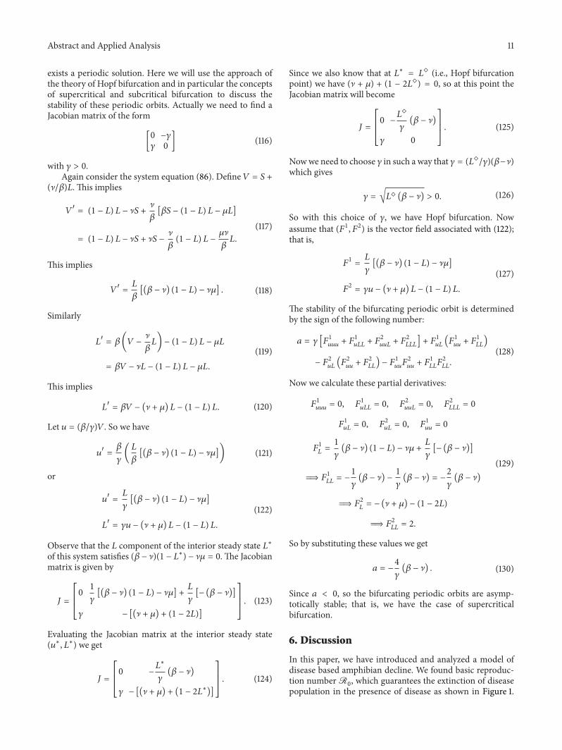
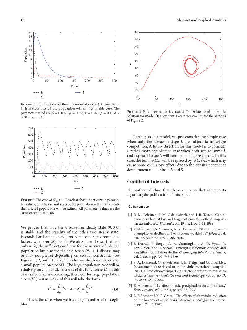
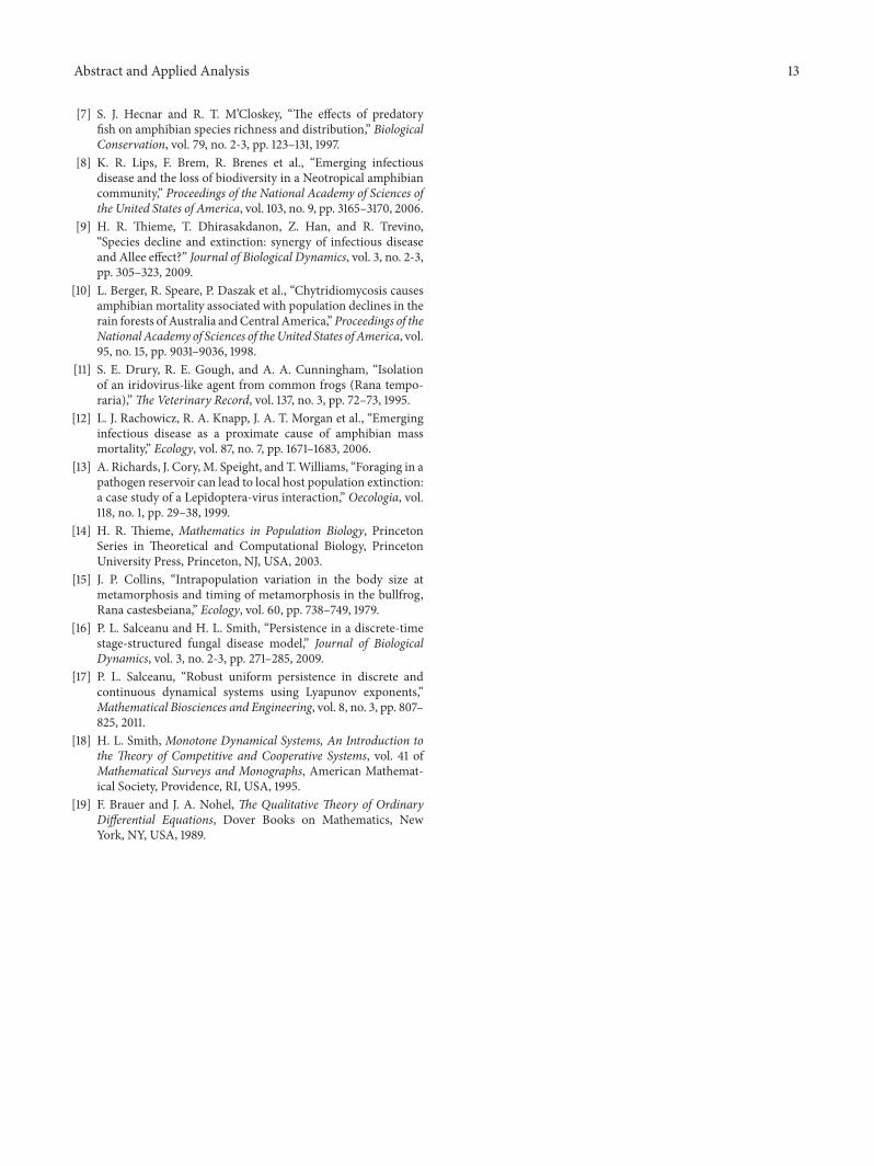