Vol. 00, No. 00, May 2010, 1–20

RESEARCH ARTICLE

Adaptive Finite Element method for a coefficient inverse problem

for the Maxwell’s system

Larisa Beilina∗

Department of Mathematical Sciences, Chalmers University of Technology and

Gothenburg University, SE-42196 Gothenburg, Sweden(Received 00 Month 200x; in final form 00 Month 200x)

We consider a coefficient inverse problems for the Maxwell’ system in 3-D. The coefficientof interest is the dielectric permittivity function. Only backscattering single measurementdata are used. The problem is formulated as an optimization problem. The key idea is to usethe adaptive finite element method for the solution. Both analytical and numerical resultsare presented. Similar ideas for inverse problems for the complete time dependent Maxwell’ssystem were not considered in the past.

Keywords: Time-dependent inverse electromagnetic scattering, adaptive finite elementmethods, a posteriori error estimation.

AMS Subject Classification: 65M15, 65M32, 65M50, 65M60

1. Introduction

In this work we consider an adaptive hybrid finite element/difference method foran electromagnetic coefficient inverse problem (CIP) in the form of a parameteridentification problem. Our goal is reconstruct dielectric permittivity ǫ of the me-dia under condition that magnetic permeability µ = 1. We consider the case of asingle measurement and use the backscattering data only to reconstruct this coef-ficient ǫ. Potential applications of our algorithm are in airport security, imaging ofland mines, imaging of defects in non-destructive testing, etc.. This is because thedielectric constants of explosives are much higher than ones of regular materials,see tables in http://www.clippercontrols.com/info/dielectric constants.html.

To solve our inverse problem numerically, we seek to minimize the Tikhonovfunctional:

F (E, ǫ) =1

2‖E − E‖2 +

1

2γ‖ǫ− ǫ0‖2. (1.1)

Here E is the vector of the electric field satisfying Maxwell´s equations and E isobserved data at a finite set of observation points at the backscattering side ofthe boundary, ǫ0 is the initial guess for ǫ, γ is regularization parameter (Tikhonovregularization), and ‖ · ‖ is the discrete L2 norm. The data E in our computationsare generated in experiments, where short electromagnetic impulses are emitted

∗ Email: larisa.beilina@chalmers.se

ISSN: 0003-6811 print/ISSN 1563-504X onlinec© 2010 Taylor & FrancisDOI: 10.1080/0003681YYxxxxxxxxhttp://www.informaworld.com

on the part of the boundary of the surrounding media. The goal is to recover theunknown spatially distributed function ǫ from the recorded boundary data E.

The minimization problem is reformulated as the problem of finding a stationarypoint of a Lagrangian involving a forward equation (the state equation), a back-ward equation (the adjoint equation) and an equation expressing that the gradientwith respect to the coefficient ǫ vanishes. To approximately obtain the value of ǫ,we arrange an iterative process via solving in each step the forward and backwardequations and updating the coefficient ǫ. In our numerical example the regular-ization parameter γ [13, 32, 33] is chosen experimentally on the basis of the bestperformance. An analytical study of the question of the choice of the regularizationparameter is outside of the scope of this publication. We refer to [17] for a detailedanalysis of this interesting topic for the adaptivity technique.

The aim of this work is to derive a posteriori error estimate for our CIP andpresent a numerical example of an accurate reconstruction using adaptive errorcontrol. Following Johnson et al. [4, 5, 14, 16, 22], and related works, we shallderive a posteriori error estimate for the Lagrangian involving the residuals ofthe state equation, adjoint state equation and the gradient with respect to ǫ. Inthis work we use the called all-at-once approach to find Frechet derivative for theTikhonov functional. Rigorous derivation of the Frechet derivatives for state andadjoint problems as well as of the Frechet derivative of the Tikhonov functionalwith respect to the coefficient can be performed similarly with [7, 8] and will bedone in a forthcoming publication.

Given a finite element mesh, a posteriori error analysis shows subdomains wherethe biggest error of the computed solution is. Thus, one needs to refine mesh inthose subdomains. It is important that a posteriori error analysis does not needa priori knowledge of the solution. Instead it uses only an upper bound of thesolution. In the case of classic forward problems, upper bounds are obtained froma priori estimates of solutions [1]. In the case of CIPs, upper bounds are assumedto be known in advance, which goes along well with the Tikhonov concept forill-posed problems [13, 33].

A posteriori error analysis addresses the main question of the adaptivity: Whereto refine the mesh? In the case of classic forward problems this analysis providesupper estimates for differences between computed and exact solutions locally, insubdomains of the original domain, see, e.g. [1, 14–16, 31]. In the case of a forwardproblem, the main factor enabling to conduct a posteriori error analysis is the well-posedness of this problem. However, every CIP is non-linear and ill-posed. Becauseof that, an estimate of the difference between computed and exact coefficients isreplaced by a posteriori estimate of the accuracy of either the Lagrangian [3, 6, 17]or of the Tikhonov functional [7]. Nevertheless, it was shown in the recent publica-tions [4, 8] that an estimate of the accuracy of the reconstruction of the unknowncoefficient is possible in CIPs (in particular, see subsection 2.3 and Theorems 7.3and 7.4 of [8]).

An outline of the work is following: in Section 2.1 we recall Maxwell´s equationsand in Section 2.2 we present the constrained formulation of Maxwell´s equations.In Section 3 we formulate our CIP and in Section 4 we introduce the finite elementdiscretization. In Section 5 we present a fully discrete version used in the computa-tions. Next, in Section 6 we establish a posteriori error estimate and formulate theadaptive algorithm. Finally, in Section 7 we present computational results demon-strating the effectiveness of the adaptive finite element/difference method on aninverse scattering problem in three dimensions.

2. Statements of forward and inverse problems

2.1. Maxwell’s equations

The electromagnetic equations in an inhomogeneous isotropic case in the boundeddomain Ω ⊂ Rd, d = 2, 3 with boundary ∂Ω are described by the first order systemof partial differential equations

∂D

∂t−∇×H = −J, in Ω × (0, T ),

∂B

∂t+ ∇×E = 0, in Ω × (0, T ),

D = ǫE,

B = µH,

E(x, 0) = E0(x),

H(x, 0) = H0(x),

(2.1)

where E(x, t),H(x, t),D(x, t), B(x, t) are the electric and magnetic fields and theelectric and magnetic inductions, respectively, while ǫ(x) > 0 and µ(x) > 0 are thedielectric permittivity and magnetic permeability that depend on x ∈ Ω, t is thetime variable, T is some final time, and J(x, t) ∈ Rd is a (given) current density.

The electric and magnetic inductions satisfy the relations

∇ ·D = ρ, ∇ ·B = 0 in Ω × (0, T ), (2.2)

where ρ(x, t) is a given charge density.Eliminating B andD from (2.1), we obtain two independent second order systems

of partial differential equations

ǫ∂2E

∂t2+ ∇× (µ−1∇× E) = −j, (2.3)

µ∂2H

∂t2+ ∇× (ǫ−1∇×H) = ∇× (ǫ−1J), (2.4)

where j = ∂J∂t

. System (2.3)-(2.4) should be completed with appropriate initial andboundary conditions.

2.2. Constrained formulation of Maxwell´s equations

To discretize Maxwell’s equations are available different formulation. Examples arethe edge elements of Nedelec [27], the node-based first-order formulation of Leeand Madsen [24], the node-based curl-curl formulation with divergence conditionof Paulsen and Lynch [29], the node-based interior-penalty discontinuous GalerkinFEM [18]. Edge elements are probably the most satisfactory from a theoreticalpoint of view [25]; in particular, they correctly represent singular behavior atreentrant corners. However, they are less attractive for time dependent computa-tions, because the solution of a linear system is required at every time iteration.Indeed, in the case of triangular or tetrahedral edge elements, the entries of thediagonal matrix resulting from mass-lumping are not necessarily strictly positive[12]; therefore, explicit time stepping cannot be used in general. In contrast, nodal

elements naturally lead to a fully explicit scheme when mass-lumping is applied[12, 23].

In this work we consider Maxwell’s equations in convex geometry without reen-trant corners and with smooth coefficient ǫ where value of ǫ does not varies much.Since we consider applications of our method in airport security and imaging ofland mines such assumptions are natural. Thus, we are able use the node-basedcurl-curl formulation with divergence condition of Paulsen and Lynch [29]. Directapplication of standard piecewise continuous [H1(Ω)]3- conforming FE for the nu-merical solution of Maxwell’s equations can result in spurious solutions. Following[29] we supplement divergence equations for electric and magnetic fields to en-force the divergence condition and reformulate Maxwell equations as a constrainedsystem:

ǫ∂2E

∂t2+ ∇× (∇× E) − s∇(∇ · E) = −j, (2.5)

and

∂2H

∂t2+ ∇× (ǫ−1∇×H) − s∇(ǫ−1∇ ·H) = ∇× (ǫ−1J), (2.6)

respectively, where s > 0 denotes the penalty factor. Here and below we assumethat electric permeability µ = 1.

For simplicity, we consider the system (2.5) – (2.6) with homogeneous initialconditions

∂E

∂t(x, 0) = E(x, 0) = 0, in Ω, (2.7)

∂H

∂t(x, 0) = H(x, 0) = 0, in Ω, (2.8)

and perfectly conducting boundary conditions

E × n = 0, on ∂Ω × (0, T ), (2.9)

H · n = 0. on ∂Ω × (0, T ), (2.10)

where n is the outward normal vector on ∂Ω. The choice of the parameter s dependson how much emphasis one places on the gauge condition; the optimal choice iss = 1 [21, 29].

2.3. Statements of forward and inverse problems

In this work as the forward problem we consider Maxwell equation for electric fieldwith homogeneous initial conditions and perfectly conducting boundary conditions

ǫ∂2E

∂t2+ ∇× (∇× E) − s∇(∇ · E) = −j, x ∈ Ω, 0 < t < T,

∇ · (ǫE) = 0, x ∈ Ω, 0 < t < T,

∂E

∂t(x, 0) = E(x, 0) = 0, in Ω,

E × n = 0, on ∂Ω × (0, T ).

(2.11)

The inverse problem for (2.6), (2.8), (2.10) can be formulated similarly and isnot considered in this work. Let Ω ⊂ R3 be a convex bounded domain with theboundary ∂Ω ∈ C3. We assume that the coefficient ǫ (x) of equation (2.11) is suchthat

ǫ (x) ∈ [1, d] , d = const. > 1, ǫ (x) = 1 for x ∈ R3 \ Ω, (2.12)

ǫ (x) ∈ C2(R3

)

. (2.13)

We consider the followingInverse Problem. Suppose that the coefficient ǫ (x) satisfies (2.12) and (2.13),

where the number d > 1 is given. Assume that the function ǫ (x) is unknown in thedomain Ω. Determine the function ǫ (x) for x ∈ Ω, assuming that the followingfunction E (x, t) is known

E (x, t) = E (x, t) ,∀ (x, t) ∈ ∂Ω × (0,∞) . (2.14)

A priori knowledge of upper and lower bounds of the coefficient ǫ (x) correspondswell with the Tikhonov concept about the availability of a priori information for anill-posed problem [13, 33]. In applications the assumption ǫ (x) = 1 for x ∈ R3 \ Ωmeans that the target coefficient ǫ (x) has a known constant value outside of themedium of interest Ω. The function E (x, t) models time dependent measurementsof the electric wave field at the boundary of the domain of interest. In practicemeasurements are performed at a number of detectors. In this case the functionE (x, t) can be obtained via one of standard interpolation procedures, a discussionof which is outside of the scope of this publication.

3. Tikhonov functional and optimality conditions

We reformulate our inverse problem as an optimization problem, where one seek thepermittivity ǫ(x), which result in a solution of equations (2.11) with best fit to timedomain observations E, measured at a finite number of observation points. DenoteQT = Ω × (0, T ) , ST = ∂Ω × (0, T ) . Our goal is minimize Tikhonov functional

F (E, ǫ) =1

2

∫

ST

(E|ST− E)2zδ(t)dxdt +

1

2γ

∫

Ω(ǫ− ǫ0)

2 dx, (3.1)

where E is the observed electric field, E satisfies the equations (2.11) and thusdepends on ǫ, and γ is regularization parameter. Here zδ(t) is a cut-off function,which is introduced to ensure that compatibility conditions at ST ∩ t = T aresatisfied, and δ > 0 is a small number. So, we choose such a function zδ that

zδ ∈ C∞ [0, T ] , zδ (t) =

1 fort ∈ [0, T − δ] ,

0 for t ∈(

T − δ2 , T

]

,

0 < zδ < 1 for t ∈(

T − δ, T − δ2

)

.

To solve this minimization problem we introduce the Lagrangian

L(u) = F (E, ǫ) −∫

ΩT

ǫ∂λ

∂t

∂E

∂tdxdt +

∫

ΩT

(∇× E)(∇× λ) dxdt

+

∫

ΩT

∇ · (ǫE)λ dxdt+ s

∫

ΩT

(∇ ·E)(∇ · λ) dxdt+

∫

ΩT

jλ dxdt,

(3.2)

where u = (E,λ, ǫ), and search for a stationary point with respect to u satisfying∀u = (E, λ, ǫ)

L′(u; u) = 0, (3.3)

where L′(u; ·) is the Jacobian of L at u.We assume that λ (x, T ) = ∂tλ (x, T ) = 0 and seek to impose such conditions

on the function λ that in (3.2) L (E,λ, ǫ) := L (u) = F (E, ǫ) . In other words, thesum of integral terms in (3.2) should be equal to zero. Then we will come up withthe formulation of the so-called adjont problem for the function λ.

To proceed further we use the fact that λ(x, T ) = ∂λ∂t

(x, T ) = 0 and E(x, 0) =∂E∂t

(x, 0) = 0, together with perfectly conducting boundary conditions n × E =n× λ = 0 and n · (∇ · E) = n · E = n · (ǫE) = 0 and n · (∇ · λ) = n · λ = 0 on ∂Ω.The equation (3.3) expresses that for all u,

0 =∂L

∂λ(u)(λ) = −

∫

ΩT

ǫ∂λ

∂t

∂E

∂tdxdt+

∫

ΩT

(∇× E)(∇× λ) dxdt

+ s

∫

ΩT

(∇ ·E)(∇ · λ) dxdt +

∫

ΩT

∇ · (ǫE)λ dxdt +

∫

ΩT

jλ dxdt,

(3.4)

0 =∂L

∂E(u)(E) =

∫

ΩT

(E − E) E zδ dxdt

−∫

ΩT

ǫ∂λ

∂t

∂E

∂tdxdt +

∫

ΩT

(∇× λ)(∇× E) dxdt

+ s

∫

ΩT

(∇ · λ)(∇ · E) dxdt−∫

ΩT

ǫ∇λE dxdt,

(3.5)

0 =∂L

∂ǫ(u)(ǫ) = −

∫

ΩT

∂λ

∂t

∂E

∂tǫ dxdt−

∫

ΩT

E∇λǫ dxdt+ γ

∫

Ω(ǫ− ǫ0)ǫ dx, x ∈ Ω,

(3.6)The equation (3.4) is the weak formulation of the state equation (2.5) and the

equation (3.5) is the weak formulation of the following adjoint problem

ǫ∂2λ

∂t2+ ∇× (∇× λ) − s∇(∇ · λ) = −(E − E)zδ, x ∈ Ω, 0 < t < T,

∇ · (ǫλ) = 0, x ∈ Ω, 0 < t < T,

λ(·, T ) =∂λ

∂t(·, T ) = 0,

λ× n = 0 on ST .

(3.7)

Further, (3.6) expresses stationarity with respect to ǫ.

4. Finite element discretization

We discretize Ω × (0, T ) denoting by Kh = K a partition of the domain Ω intotetrahedra K (h = h(x) being a mesh function defined as h|K = hK representingthe local diameter of the elements), and we let Jk be a partition of the time interval(0, T ) into time intervals J = (tk−1, tk] of uniform length τ = tk − tk−1. We assumealso a minimal angle condition on the Kh [9].

To formulate the finite element method for (3.3) we introduce the finite elementspaces Vh, WE

h and W λh defined by :

Vh := v ∈ L2(Ω) : v ∈ P0(K),∀K ∈ Kh,

WE := w ∈ [H1(Ω × I)]3 : w(·, 0) = 0, w × n|∂Ω = 0,

WEh := w ∈WE : w|K×J ∈ [P1(K) × P1(J)]3,∀K ∈ Kh,∀J ∈ Jk,

W λ := w ∈ [H1(Ω × I)]3 : w(·, T ) = 0, w × n|∂Ω = 0,

W λh := w ∈W λ : w|K×J ∈ [P1(K) × P1(J)]3,∀K ∈ Kh,∀J ∈ Jk,

where P1(K) and P1(J) are the set of continuous piecewise linear functions on Kand J , respectively.

We define Uh = WEh × W λ

h × Vh. The finite element method now reads: Finduh ∈ Uh, such that

L′(uh)(u) = 0 ∀u ∈ Uh. (4.1)

5. Fully discrete scheme

We expand E,λ in terms of the standard continuous piecewise linear functionsϕi(x) in space and ψi(t) in time and substitute this into (2.11) and (3.7) to obtainthe following system of linear equations:

M(Ek+1 − 2Ek + Ek−1) = −τ2F k − τ2KEk − sτ2CEk − τ2BEk,

M(λk+1 − 2λk + λk−1) = −τ2Sk − τ2Kλ

k − sτ2Cλk − τ2Bλ

k,(5.1)

with initial conditions :

E(·, 0) = ∂E∂t

(·, 0) = 0, (5.2)

λ(·, T ) = ∂λ∂t

(·, T ) = 0. (5.3)

Here, M is the block mass matrix in space, K is the block stiffness matrix corre-sponding to the rotation term, C and B are the stiffness matrices correspondingto the divergence terms, F k and Sk are the load vectors at time level tk, Ek andλ

k denote the nodal values of E(·, tk) and λ(·, tk), respectively, τ is the time step.The explicit formulas for the entries in system (5.1) at each element e can be

given as:

Mei,j = (ǫ ϕi, ϕj)e,

Kei,j = (

1

µ∇× ϕi,∇× ϕj)e,

Cei,j = (

1

µ∇ · ϕi,∇ · ϕj)e,

Bei,j = (∇ · (ǫϕi), ϕj)e,

F ej,m = ((j, ϕjψm))e×J ,

Sej,m = ((E − E, ϕjψm))e×J ,

(5.4)

where (·, ·)e denotes the L2(e) scalar product.To obtain an explicit scheme we approximate M with the lumped mass matrix

ML – see [10, 20, 23]. Next, we multiply (5.1) with (ML)−1 and get the followingexplicit method:

Ek+1 = − τ2(ML)−1F k + 2Ek − τ2(ML)−1KEk

− sτ2(ML)−1CEk − τ2(ML)−1BEk − Ek−1,

λk−1 = − τ2(ML)−1Sk + 2λk − τ2(ML)−1Kλ

k

− sτ2(ML)−1Cλk − τ2(ML)−1Bλ

k − λk+1.

(5.5)

Finally, to approximate coefficient ǫ can be used one of the gradient-like methodswith an appropriate initial guess value ǫ0. The discrete version of gradient withrespect to the coefficient (3.6) takes the form:

gh = −∫

0

T ∂λkh

∂t

∂Ekh

∂tdxdt−

∫ T

0Ek

h∇λkhdt+ γ(ǫkh − ǫ0). (5.6)

Here, λkh and EK

h are computed values of the adjoint and forward problems attime moment k using explicit scheme (5.5), and ǫkh is approximated value of thecoefficient.

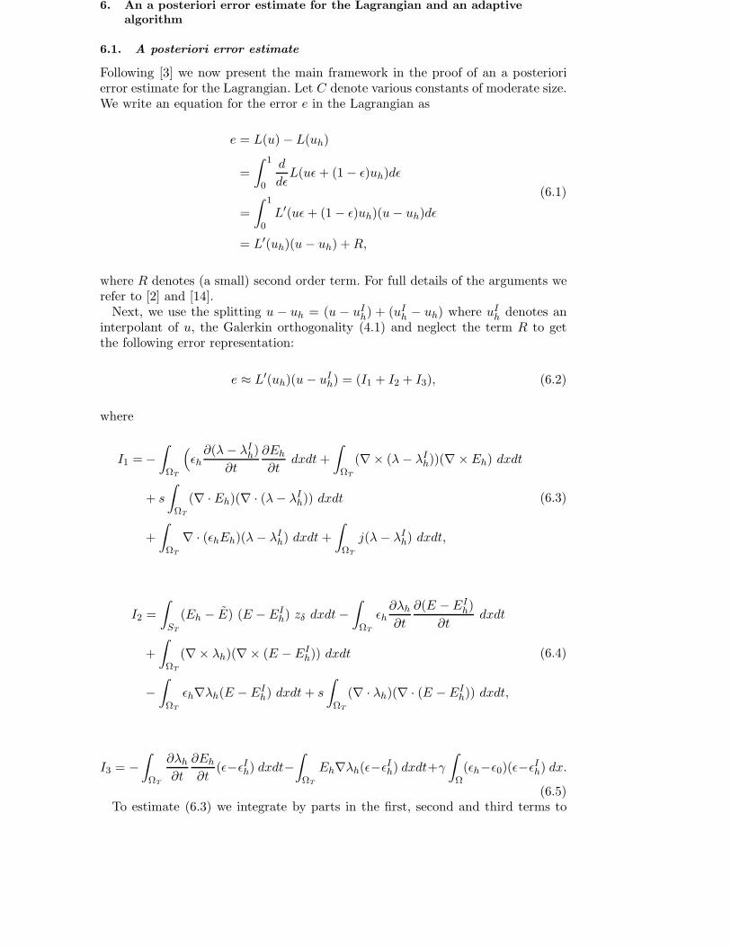
6. An a posteriori error estimate for the Lagrangian and an adaptive

algorithm

6.1. A posteriori error estimate

Following [3] we now present the main framework in the proof of an a posteriorierror estimate for the Lagrangian. Let C denote various constants of moderate size.We write an equation for the error e in the Lagrangian as

e = L(u) − L(uh)

=

∫ 1

0

d

dǫL(uǫ+ (1 − ǫ)uh)dǫ

=

∫ 1

0L′(uǫ+ (1 − ǫ)uh)(u− uh)dǫ

= L′(uh)(u− uh) +R,

(6.1)

where R denotes (a small) second order term. For full details of the arguments werefer to [2] and [14].

Next, we use the splitting u − uh = (u − uIh) + (uI

h − uh) where uIh denotes an

interpolant of u, the Galerkin orthogonality (4.1) and neglect the term R to getthe following error representation:

e ≈ L′(uh)(u− uIh) = (I1 + I2 + I3), (6.2)

where

I1 = −∫

ΩT

(

ǫh∂(λ− λI

h)

∂t

∂Eh

∂tdxdt+

∫

ΩT

(∇× (λ− λIh))(∇ ×Eh) dxdt

+ s

∫

ΩT

(∇ · Eh)(∇ · (λ− λIh)) dxdt

+

∫

ΩT

∇ · (ǫhEh)(λ− λIh) dxdt +

∫

ΩT

j(λ − λIh) dxdt,

(6.3)

I2 =

∫

ST

(Eh − E) (E − EIh) zδ dxdt−

∫

ΩT

ǫh∂λh

∂t

∂(E − EIh)

∂tdxdt

+

∫

ΩT

(∇× λh)(∇× (E − EIh)) dxdt

−∫

ΩT

ǫh∇λh(E − EIh) dxdt + s

∫

ΩT

(∇ · λh)(∇ · (E − EIh)) dxdt,

(6.4)

I3 = −∫

ΩT

∂λh

∂t

∂Eh

∂t(ǫ−ǫIh) dxdt−

∫

ΩT

Eh∇λh(ǫ−ǫIh) dxdt+γ

∫

Ω(ǫh−ǫ0)(ǫ−ǫIh) dx.

(6.5)To estimate (6.3) we integrate by parts in the first, second and third terms to

get:

I1 =

∫

ΩT

(

ǫh∂2Eh

∂t2+ ∇× (∇×Eh) − s∇(∇ ·Eh) + ∇ · (ǫhEh) + j

)

(λ− λIh) dx dt

+∑

k

∫

Ωǫh

[∂Eh

∂t(tk)

]

(λ− λIh)(tk) dx−

∑

K

∫ T

0

∫

∂K

(

nK × (∇× Eh))

(λ− λIh) dsdt

+ s∑

K

∫ T

0

∫

∂K

(∇ · Eh) (nK · (λ− λIh)) dS dt = J1 + J2 + J3 + J4,

(6.6)

where Ji, i = 1, ..., 4 denote integrals that appear on the right of (6.6). In particular,J2, J3 result from integration by parts in space, whereas

[

∂Eh

∂t

]

appears during theintegration by parts in time and denotes the jump of the derivative of Eh in time.Here nK denotes the exterior unit normal to element K.

To estimate J3 we sum over the element boundaries where each internal sideS ∈ Sh occurs twice. Let Es denote the function Eh in one of the normal directionsof each side S and ns is outward normal vector on S. Then we can write

∑

K

∫

∂K

(

nK×(∇×Eh))

(λ−λIh) dS =

∑

S

∫

S

[

nS×(∇×ES)]

(λ−λIh) dS, (6.7)

where[

nS × (∇× Es)]

is the tangential jump of ∇× Eh computed from the two

elements sharing S. We distribute each jump equally to the two sharing trianglesand return to a sum over all element edges ∂K as :

∑

S

∫

S

[

nS×(∇×Es)]

(λ−λIh) dS =

∑

K

1

2h−1

K

∫

∂K

[

nS×(∇×Es)]

(λ−λIh)hK dS.

(6.8)We formally set dx = hKdS and replace the integrals over the element boundaries∂K by integrals over the elements K, to get:

∣

∣

∣

∑

K

1

2h−1

K

∫

∂K

[

nS×(∇×Es)]

(λ−λIh)hK dS

∣

∣

∣≤ C

∫

ΩmaxS⊂∂K

h−1K

∣

∣

∣

[

nK×(∇×Eh)]∣

∣

∣·∣

∣

∣λ−λI

h

∣

∣

∣dx,

(6.9)

with[

nK × (∇×Eh)]∣

∣

∣

K= maxS⊂∂K

[

nS × (∇×Es)]∣

∣

∣

S. Here and later we denote

by C different constants of moderate size.In a similar way we can estimate J4 in (6.6):

J4 = s∑

K

∫

∂K

(∇ ·Eh) (nK · (λ− λIh)) as

= s∑

S

∫

S

[∇ · Es] [nS · (λ− λIh)] dS

= s∑

K

1

2h−1

K

∫

∂K

[∇ · Es] [nS · (λ− λIh)]hK dS.

(6.10)

Again, replacing the integrals over the boundaries by integrals over the elements

we get the following estimate for J4:

∣

∣

∣J4

∣

∣

∣≤ s C

∫

ΩmaxS⊂∂K

h−1K

∣

∣

∣[∇ ·Eh]

∣

∣

∣·∣

∣

∣[nK · (λ− λI

h)]∣

∣

∣dx, (6.11)

with [∇ ·Eh]∣

∣

∣

K= maxS⊂∂K [∇ ·Es]

∣

∣

∣

S. J2 is estimated similarly with J3, J4.

We substitute expressions for J2, J3 and J4 in (6.6) to get:

∣

∣I1∣

∣ ≤∫

ΩT

∣

∣

∣

(

ǫh∂2Eh

∂t2+ ∇× (∇× Eh) − s∇(∇ · Eh) + ∇ · (ǫhEh) + j

)∣

∣

∣·∣

∣

∣λ− λI

h

∣

∣

∣dx dt

+C

∫

ΩT

ǫhτ−1 ·

∣

∣

[

∂Eht

]∣

∣ ·∣

∣λ− λIh

∣

∣ dxdt

+C

∫

ΩT

maxS⊂∂K

h−1K ·

∣

∣

∣

[

nK × (∇× Eh)]∣

∣

∣·∣

∣

∣λ− λI

h

∣

∣

∣dxdt

+ s C

∫

ΩT

maxS⊂∂K

h−1K ·

∣

∣

[

∇ · Eh

]∣

∣ ·∣

∣

∣

[

nK · (λ− λIh)

]∣

∣

∣dxdt.

(6.12)

where

[∂Eht] = [∂Ehtk] on Jk

and [∂Ehtk] is defined as the maximum of the two jumps in time on each time

interval Jk:

[∂Ehtk] = max

Jk

([

∂Eh

∂t(tk)

]

,

[

∂Eh

∂t(tk+1)

])

. (6.13)

Next, we use a standard interpolation estimate [3] for λ− λIh to get

∣

∣I1∣

∣ ≤∫

ΩT

∣

∣

∣

(

ǫh∂2Eh

∂t2+ ∇× (∇× Eh) − s∇(∇ · Eh) + ∇ · (ǫhEh) + j

)∣

∣

∣·(

τ2

∣

∣

∣

∣

∂2λ

∂t2

∣

∣

∣

∣

+ h2∣

∣D2xλ

∣

∣

)

dx dt

+C

∫

ΩT

ǫhτ−1 ·

∣

∣

[

∂Eht

]∣

∣ ·(

τ2

∣

∣

∣

∣

∂2λ

∂t2

∣

∣

∣

∣

+ h2∣

∣D2xλ

∣

∣

)

dxdt

+C

∫

ΩT

maxS⊂∂K

h−1K ·

∣

∣

∣

[

nK × (∇× Eh)]∣

∣

∣·(

τ2

∣

∣

∣

∣

∂2λ

∂t2

∣

∣

∣

∣

+ h2∣

∣D2xλ

∣

∣

)

dxdt

+ s C

∫

ΩT

maxS⊂∂K

h−1K ·

∣

∣

[

∇ · Eh

]∣

∣ ·[

nK ·(

τ2

∣

∣

∣

∣

∂2λ

∂t2

∣

∣

∣

∣

+ h2∣

∣D2xλ

∣

∣

)]

dxdt.

(6.14)

Next, in (6.14) the terms ∂2Eh

∂t2,∇ × (∇ × Eh),∇(∇ · Eh) vanish, since Eh is

continuous piecewise linear function. We then estimate ∂2λ∂t2

≈[

∂λh

∂t

]

τand D2

xλ ≈

[

∂λh

∂n

]

hto get:

∣

∣I1∣

∣ ≤ C

∫

ΩT

∣

∣j + ∇ · (ǫhEh)∣

∣ ·(

τ2∣

∣

∣

[

∂λh

∂t

]

τ

∣

∣

∣+ h2

∣

∣

∣

[

∂λh

∂n

]

h

∣

∣

∣

)

dxdt

+ C

∫

ΩT

ǫhτ−1

∣

∣

[

∂Eht

]∣

∣ ·(

τ2∣

∣

∣

[

∂λh

∂t

]

τ

∣

∣

∣+ h2

∣

∣

∣

[

∂λh

∂n

]

h

∣

∣

∣

)

dxdt

+ C

∫

ΩT

maxS⊂∂K

h−1K ·

∣

∣

∣

[

nK × (∇× Eh)]∣

∣

∣·(

τ2∣

∣

∣

[

∂λh

∂t

]

τ

∣

∣

∣+ h2

∣

∣

∣

[

∂λh

∂n

]

h

∣

∣

∣

)

dxdt

+ s C

∫

ΩT

maxS⊂∂K

h−1K ·

∣

∣

[

∇ ·Eh

]∣

∣ ·[

nK ·(

τ2∣

∣

∣

[

∂λh

∂t

]

τ

∣

∣

∣+ h2

∣

∣

∣

[

∂λh

∂n

]

h

∣

∣

∣

)]

dxdt.

(6.15)

We estimate I2 similarly:

∣

∣I2∣

∣ ≤∫

ΩT

∣

∣

∣

(

ǫh∂2λh

∂t2+ ∇× (∇× λh) − ǫhλh − s∇(∇ · λh)

)

∣

∣

∣·∣

∣

∣E − EI

h

∣

∣

∣dxdt

+

∫

ST

∣

∣

∣Eh − E

∣

∣

∣·∣

∣

∣E − EI

h

∣

∣

∣zδ dxdt+

∣

∣

∣

∑

k

∫

Ωǫh

[∂λh

∂t(tk)

]

(E − EIh)(tk) dx

∣

∣

∣

+∣

∣

∣

∑

K

∫ T

0

∫

∂K

(

nK × (∇× λh))

(E −EIh) dSdt

∣

∣

∣

+ s∑

K

∫ T

0

∫

∂K

(∇ · λh) (nK · (E −EIh)) dS dt

∣

∣

∣.

(6.16)

Next, we can estimate (6.16) similarly with (6.15) as

∣

∣I2∣

∣ ≤∫

ΩT

∣

∣

∣

∣

(

ǫh∂2λh

∂t2+ ∇× (∇× λh) − ǫh∇λh − s∇(∇ · λh)

)∣

∣

∣

∣

·∣

∣E − EIh

∣

∣ dxdt

+

∫

ST

∣

∣Eh − E∣

∣ ·∣

∣E − EIh

∣

∣ zδ dxdt

+ C

∫

ΩT

ǫhτ−1 ·

∣

∣

[

∂λht

]∣

∣ ·∣

∣E − EIh

∣

∣ dxdt

+ C

∫

ΩT

maxS⊂∂K

h−1K ·

∣

∣

∣

[

nK × (∇× λh)]∣

∣

∣·∣

∣

∣E − EI

h

∣

∣

∣dxdt

+ s C

∫

ΩT

maxS⊂∂K

h−1K ·

∣

∣

[

∇ · λh

]∣

∣ ·∣

∣

∣

[

nK · (E − EIh)

]∣

∣

∣dxdt.

(6.17)

Again, the terms ∂2λh

∂t2,∇× (∇× λh),∇(∇ · λh) vanish, since λh is also continuous

piecewise linear function. Finally we get

∣

∣I2∣

∣ ≤∫

ΩT

∣

∣ǫh∇λh

∣

∣ ·(

τ2∣

∣

∣

[

∂Eh

∂t

]

τ

∣

∣

∣+ h2

∣

∣

∣

[

∂Eh

∂n

]

h

∣

∣

∣

)

dxdt

+

∫

ST

∣

∣Eh − E∣

∣ ·(

τ2∣

∣

∣

[

∂Eh

∂t

]

τ

∣

∣

∣+ h2

∣

∣

∣

[

∂Eh

∂n

]

h

∣

∣

∣

)

zδ dxdt

+ C

∫

ΩT

ǫhτ−1 ·

∣

∣

[

∂λht

]∣

∣ ·(

τ2∣

∣

∣

[

∂Eh

∂t

]

τ

∣

∣

∣+ h2

∣

∣

∣

[

∂Eh

∂n

]

h

∣

∣

∣

)

dxdt

+ C

∫

ΩT

maxS⊂∂K

h−1K ·

∣

∣

∣

[

nK × (∇× λh)]∣

∣

∣·(

τ2∣

∣

∣

[

∂Eh

∂t

]

τ

∣

∣

∣+ h2

∣

∣

∣

[

∂Eh

∂n

]

h

∣

∣

∣

)

dxdt

+ s C

∫

ΩT

maxS⊂∂K

h−1K ·

∣

∣

[

∇ · λh

]∣

∣ ·[

nK ·(

τ2∣

∣

∣

[

∂Eh

∂t

]

τ

∣

∣

∣+ h2

∣

∣

∣

[

∂Eh

∂n

]

h

∣

∣

∣

)]

dxdt.

(6.18)

To estimate I3 we use a standard approximation estimate in the form ǫ − ǫIh ≈hDxǫ to get:

∣

∣

∣I3

∣

∣ ≤ C

∫

ΩT

∣

∣

∣

∂λh

∂t

∣

∣

∣·∣

∣

∣

∂Eh

∂t

∣

∣

∣· h

∣

∣Dxǫ∣

∣ dxdt +C

∫

ΩT

∣

∣

∣Eh

∣

∣

∣·∣

∣

∣∇λh

∣

∣

∣· h

∣

∣Dxǫ∣

∣ dxdt

+ γ C

∫

Ω|ǫh − ǫ0| · h

∣

∣

∣Dxǫ

∣

∣

∣dx

≤ C

∫ T

0

∫

Ω

∣

∣

∣

∂λh

∂t

∣

∣

∣·∣

∣

∣

∂Eh

∂t

∣

∣

∣· h

∣

∣

∣

[ǫh]

h

∣

∣

∣dxdt+ C

∫

ΩT

∣

∣

∣Eh

∣

∣

∣·∣

∣

∣∇λh

∣

∣

∣· h

∣

∣

∣

[ǫh]

h

∣

∣

∣dxdt

+ γ C

∫

Ω|ǫh − ǫ0| · h

∣

∣

∣

[ǫh]

h

∣

∣

∣dx

≤ C

∫ T

0

∫

Ω

∣

∣

∣

∂λh

∂t

∣

∣

∣·∣

∣

∣

∂Eh

∂t

∣

∣

∣·∣

∣[ǫh]∣

∣ dxdt + C

∫

ΩT

∣

∣

∣Eh

∣

∣

∣·∣

∣

∣∇λh

∣

∣

∣·∣

∣

∣[ǫh]

∣

∣

∣dxdt

+ γ C

∫

Ω|ǫh − ǫ0| ·

∣

∣[ǫh]∣

∣ dx.

(6.19)

We therefore obtain the following:

Theorem 5.1 Let L(u) = L(E,λ, ǫ) be the Lagrangian defined in (3.2), andlet L(uh) = L(Eh, λh, ǫh) be the approximation of L(u). Then the following errorrepresentation formula for the error e = L(u) − L(uh) in the Lagrangian holds:

∣

∣e∣

∣ ≤3

∑

i=1

∫

ΩT

REiσλ1

dxdt +

∫

ΩT

RE4σλ2

dxdt +

∫

ST

Rλ1σE1

zδ dxdt

+4

∑

i=2

∫

ΩT

RλiσE1

dxdt +

∫

ΩT

Rλ5σE2

dxdt +3

∑

i=1

∫

ΩT

Rǫiσǫ dxdt,

(6.20)

where residuals are defined by

RE1=

∣

∣j + ∇ · (ǫhEh)∣

∣, RE2= ǫhτ

−1∣

∣

[

∂Eht

]∣

∣, RE3= max

S⊂∂Kh−1

K

∣

∣

∣

[

nK × (∇× Eh)]∣

∣

∣,

RE4= s max

S⊂∂Kh−1

K

∣

∣

[

∇ · Eh

]∣

∣,

Rλ1=

∣

∣Eh − E∣

∣, Rλ2= |ǫh∇λh|, Rλ3

= ǫhτ−1

∣

∣

[

∂λht

]∣

∣,

Rλ4= max

S⊂∂Kh−1

K

∣

∣

∣

[

nK × (∇× λh)]∣

∣

∣, Rλ5

= s maxS⊂∂K

h−1K

∣

∣

[

∇ · λh

]∣

∣,

Rǫ1 =

∣

∣

∣

∣

∂λh

∂t

∣

∣

∣

∣

·∣

∣

∣

∣

∂Eh

∂t

∣

∣

∣

∣

, Rǫ2 = |Eh| · |∇λh|, Rǫ3 = γ |ǫh − ǫ0|,

and interpolation errors are

σλ1= C

(

τ∣

∣

∣

[∂λh

∂t

]∣

∣

∣+ h

∣

∣

∣

[∂λh

∂n

]∣

∣

∣

)

, σλ2= C

[

nK ·(

τ∣

∣

∣

[∂λh

∂t

]∣

∣

∣+ h

∣

∣

∣

[∂λh

∂n

]∣

∣

∣

)]

,

σE1= C

(

τ∣

∣

∣

[∂Eh

∂t

]∣

∣

∣+ h

∣

∣

∣

[∂Eh

∂n

]∣

∣

∣

)

, σE2= C

[

nK ·(

τ∣

∣

∣

[∂Eh

∂t

]∣

∣

∣+ h

∣

∣

∣

[∂Eh

∂n

]∣

∣

∣

)]

,

σǫ = C∣

∣[ǫh]∣

∣.

Remark 5.1

If solutions λh and Eh to the adjoint and state equations are computedwith good accuracy, then we can neglect terms

∑4i=1

∫

ΩT

REiσλ1

dxdt +∑5

i=1

∫

ΩT

RλiσE1

dxdt +∫

ΩT

Rǫ2σǫ dxdt in a posteriori error estimation (6.20).Thus the term

N(ǫh) =∣

∣

∣

∫ T

0

∂λh

∂t

∂Eh

∂tdt+ γ (ǫh − ǫ0)

∣

∣

∣(6.21)

dominates. This fact is also observed numerically (see next section) and will beexplained analytically in forthcoming publication.

Mesh refinement recommendation

From the Theorem 5.1 and Remark 5.1 follows that the mesh should be refinedin such subdomain of the domain Ω where values of the function N(ǫh) are closeto the number

maxΩ

|N(ǫh)| = maxΩ

∣

∣

∣

∫ T

0

∂λh

∂t

∂Eh

∂tdt+ γ (ǫh − ǫ0)

∣

∣

∣. (6.22)

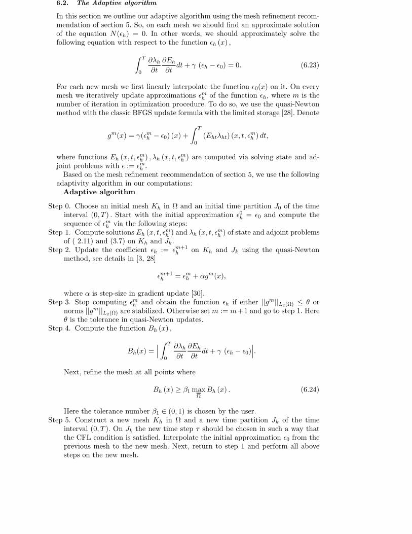
6.2. The Adaptive algorithm

In this section we outline our adaptive algorithm using the mesh refinement recom-mendation of section 5. So, on each mesh we should find an approximate solutionof the equation N(ǫh) = 0. In other words, we should approximately solve thefollowing equation with respect to the function ǫh (x) ,

∫ T

0

∂λh

∂t

∂Eh

∂tdt+ γ (ǫh − ǫ0) = 0. (6.23)

For each new mesh we first linearly interpolate the function ǫ0(x) on it. On everymesh we iteratively update approximations ǫmh of the function ǫh, where m is thenumber of iteration in optimization procedure. To do so, we use the quasi-Newtonmethod with the classic BFGS update formula with the limited storage [28]. Denote

gm(x) = γ(ǫmh − ǫ0) (x) +

∫ T

0(Ehtλht) (x, t, ǫmh ) dt,

where functions Eh (x, t, ǫmh ) , λh (x, t, ǫmh ) are computed via solving state and ad-joint problems with ǫ := ǫmh .

Based on the mesh refinement recommendation of section 5, we use the followingadaptivity algorithm in our computations:

Adaptive algorithm

Step 0. Choose an initial mesh Kh in Ω and an initial time partition J0 of the timeinterval (0, T ) . Start with the initial approximation ǫ0h = ǫ0 and compute thesequence of ǫmh via the following steps:

Step 1. Compute solutions Eh (x, t, ǫmh ) and λh (x, t, ǫmh ) of state and adjoint problemsof ( 2.11) and (3.7) on Kh and Jk.

Step 2. Update the coefficient ǫh := ǫm+1h on Kh and Jk using the quasi-Newton

method, see details in [3, 28]

ǫm+1h = ǫmh + αgm(x),

where α is step-size in gradient update [30].Step 3. Stop computing ǫmh and obtain the function ǫh if either ||gm||L2(Ω) ≤ θ or

norms ||gm||L2(Ω) are stabilized. Otherwise set m := m+1 and go to step 1. Hereθ is the tolerance in quasi-Newton updates.

Step 4. Compute the function Bh (x) ,

Bh(x) =∣

∣

∣

∫ T

0

∂λh

∂t

∂Eh

∂tdt+ γ (ǫh − ǫ0)

∣

∣

∣.

Next, refine the mesh at all points where

Bh (x) ≥ β1 maxΩ

Bh (x) . (6.24)

Here the tolerance number β1 ∈ (0, 1) is chosen by the user.Step 5. Construct a new mesh Kh in Ω and a new time partition Jk of the time

interval (0, T ). On Jk the new time step τ should be chosen in such a way thatthe CFL condition is satisfied. Interpolate the initial approximation ǫ0 from theprevious mesh to the new mesh. Next, return to step 1 and perform all abovesteps on the new mesh.

Step 6. Stop mesh refinements if norms defined in step 3 either increase or stabilize,compared with the previous mesh.

7. Numerical example

We test the performance of the adaptive algorithm formulated above on the solu-tion of an inverse electromagnetic scattering problem in three dimensions. In ourcomputational example we consider the domain Ω = [−9.0, 9.0] × [−10.0,−12.0] ×[−9.0, 9.0] with an unstructured mesh consisting of tetrahedra. The domain Ω issplit into inner domain Ω1 which contains scatterer, and surrounding outer domainΩ2 such that Ω = Ω1∪Ω2. The spherical part of the boundary of the domain Ω1 wedenote as ∂Ω1 and the boundary of the domain Ω we denote as ∂Ω. The domainΩ1 is a cylinder covered by spherical surface from top, see Figure 1-a). We setǫ (x) = 10 inside of the inclusion depicted on Figure 1-b) and ǫ (x) = 1 outside ofit. Hence, the inclusion/background contrast in the dielectric permittivity coeffi-cient is 10 : 1. In our computational test we chose a time step τ according to theCourant-Friedrichs-Levy (CFL) stability condition

τ ≤√ǫmaxh√

3, (7.1)

where h is the minimal local mesh size, ǫmax is an upper bound for the coefficientǫ.

The forward problem in our test is

ǫ∂2E

∂t2+ ∇× (∇× E) − s∇(∇ ·E) = 0, x ∈ Ω, 0 < t < T,

∇ · (ǫE) = 0, x ∈ Ω, 0 < t < T,

∂E

∂t(x, 0) = E(x, 0) = 0, in Ω,

E × n = f(t), on ∂Ω1 × [0, t1],

E × n = 0, on ∂Ω1 × (t1, T ],

E × n = 0, on ∂Ω × [0, T ].

(7.2)

Let Ω1 ⊂ R3 be a convex bounded domain which is split into upper Ωup andlower Ωdown domains such that Ω1 = Ωup ∪ Ωdown. We assume that we need toreconstruct coefficient ǫ(x) only in Ωdown from back reflected data at ∂Ω1. In otherwords we assume that the coefficient ǫ (x) of equation (7.2) is such that

ǫ (x) ∈ [1, d] , d = const. > 1, ǫ (x) = 1 for x ∈ R3 \ Ωdown, (7.3)

ǫ (x) ∈ C2(R3

)

. (7.4)

In the following example we consider the electrical field which is given as

f(t) = −((sin (100t − π/2) + 1)/10) × n, 0 ≤ t ≤ 2π

100. (7.5)

We initialize (7.5) at the spherical boundary ∂Ω1 and propagate it into Ω. The ob-servation points are placed on ∂Ω1. We note, that in actual computations applying

adaptive algorithm the number of the observations points on ∂Ω1 increases fromcoarse to finer mesh.

As follows from Theorem 5.1, to estimate the error in the Lagrangian we needto compute approximated values of (Eh, λh, ǫh) together with residuals and inter-polation errors. Since the residuals Rǫ1 , Rǫ3 dominate we neglect computations ofothers terms in a posteriori error estimate appearing in (6.20), see also Remark 5.1.We seek the solution of the optimization problem in an iterative process, where westart with a coarse mesh shown in Fig. 1, refine this mesh as in step 6 of Algorithmin section 6, and construct a new mesh and a new time partition.

To generate the data at the observation points, we solve the forward problem(7.2), with function f(t) given by (7.5) in the time interval t = [0, 36.0] with theexact value of the parameters ǫ = 10.0, µ = 1 inside scatterer, and ǫ = µ = 1.0everywhere else in Ω. We start the optimization algorithm with guess values of theparameter ǫ = 1.0 at all points in Ω. The solution of the inverse problem needs tobe regularized since different coefficients can correspond to similar wave reflectiondata on ∂Ω1. We regularize the solution of the inverse problem by introducing anregularization parameter γ (small).

The computations were performed on four adaptively refined meshes. In Fig. 2-b)we show a comparison of Rǫ1 over the time interval [25, 36] on different adaptivelyrefined meshes. Here, the smallest values of the residual Rǫ1 are shown on thecorresponding meshes.

The L2-norms in space of the adjoint solution λh on different optimization it-erations on adaptively refined meshes are shown in Fig. 2-a). Here, we solved theadjoint problem backward in time from t = 36.0 down to t = 0.0. The L2-norms arepresented on the time interval [25, 36] since the solution does not vary much on thetime interval [0, 25). We observe, that the norm of the adjoint solution decreasesfaster on finer meshes.

The reconstructed parameter ǫ on different adaptively refined meshes at the finaloptimization iteration is presented in Fig. 3. We show isosurfaces of the parameterfield ǫ(x) with a given parameter value. We observe that the qualitative value ofthe reconstructed parameter ǫ is acceptable only using adaptive error control onfiner meshes although the shape of the inclusion is reconstructed sufficiently goodon the coarse mesh.

However, since the quasi-Newton method is only locally convergent, the values ofthe identified parameters are very sensitive to the guess values of the parameters inthe optimization algorithm and also to the values of the regularization parameterγ. We use cut-off constrain on the computed parameter ǫ, as also a smoothnessindicator to update new values of the parameter ǫ by local averaging over theneighbouring elements. Namely, minimal and maximal values of the coefficient ǫ inbox constraints belongs to the following set of admissible parameters ǫ ∈ P = ǫ ∈C(Ω)|1 ≤ ǫ(x) ≤ 10.

8. Conclusions

We present and adaptive finite element method for an inverse electromagneticscattering problem. The adaptivity is based on a posteriori error estimate for theassociated Lagrangian in the form of space-time integrals of residuals multipliedby weights. We illustrate usefulness of a posteriori error indicator on an inverseelectromagnetic scattering problem in three dimensions.

a) Computational mesh b) Scatterer to be reconstructed

Figure 1. Computational domain Ω

0 50 100 150 200 2500

0.2

0.4

0.6

0.8

1

1.2

1.4

time steps

L 2 nor

m o

f the

adj

oint

sol

utio

n

22205 nodes23033 nodes24517 nodes25744 nodes

0 100 200 300 400 500 600 7000

2

4

6

8

10

12

14

16

time steps

||R1||

23033 nodes24517 nodes25744 nodes

a) b)

Figure 2. Comparison of a) ||λh|| and b) Rǫ1on different adaptively refined meshes. Here the horizontal

x-axis denotes time steps.

9. Acknowledgements

The research was partially supported by the Swedish Foundation for StrategicResearch (SSF) in Gothenburg Mathematical Modelling Center (GMMC).

a) 22205 nodes, ǫ ≈ 3.19 b) 23033 nodes, ǫ ≈ 4.84

c) 24517 nodes, ǫ ≈ 6.09 d) 25744 nodes, ǫ ≈ 7

Figure 3. Isosurfaces of the parameter ǫ on different adaptively refined meshes.

References

[1] M. Ainsworth and J. Oden, A Posteriori Error Estimation in Finite Element Analysis, New York:Wiley, 2000.

[2] R.Becker. Adaptive finite elements for optimal control problems, Habilitation thesis, 2001.[3] L. Beilina and C. Johnson. A hybrid FEM/FDM method for an inverse scattering problem. In Nu-

merical Mathematics and Advanced Applications - ENUMATH 2001. Springer-Verlag, 2001.[4] L.Beilina, C.Johnson. A posteriori error estimation in computational inverse scattering, Math.Models

and Methods in Applied Sciences, 15(1), 23-35, 2005.[5] L. Beilina, Adaptive finite element/difference method for inverse elastic scattering waves, Appl. Com-

put. Math., 2, 119-134, 2003.[6] L. Beilina and C. Clason, An adaptive hybrid FEM/FDM method for an inverse scattering problem

in scanning acoustic microscopy. SIAM J. Sci. Comp., 28, 382-402, 2006.[7] L. Beilina and M. V. Klibanov. A posteriori error estimates for the adaptivity technique for the

Tikhonov functional and global convergence for a coefficient inverse problem, Inverse Problems, 26,045012, 2010.

[8] L. Beilina, M. V. Klibanov and M. Yu. Kokurin, Adaptivity with relaxation for ill-posed problemsand global convergence for a coefficient inverse problem,Journal of Mathematical Sciences, 167 (3)279-325, 2010.

[9] S. C. Brenner and L. R. Scott, The Mathematical theory of finite element methods, Springer-Verlag,Berlin, 1994.

[10] G. C. Cohen, Highre order numerical methods for transient wave equations, Springer-Verlag, 2002.[11] J. E. Dennis and J. J. More, Quasi-Newton methods, motivation and theory, SIAM Rev., 19, 46-89,

1977.[12] A. Elmkies and P. Joly, Finite elements and mass lumping for Maxwell’s equations: the 2D case,

Numerical Analysis, C. R. Acad. Sci. Paris, 324, 1287-1293, 1997.[13] H. W. Engl, M. Hanke and A. Neubauer, Regularization of Inverse Problems (Boston: Kluwer

Academic Publishers), 2000.[14] K. Eriksson and D. Estep and C. Johnson, Computational Differential Equations, Studentlitteratur,

Lund, 1996.[15] K. Eriksson and D. Estep and C. Johnson, Applied Mathematics: Body and Soul. Calculus in Several

Dimensions, Berlin, Springer-Verlag, 2004.[16] K. Eriksson and D. Estep and C. Johnson, Introduction to adaptive methods for differential equations,

Acta Numeric., 105-158, 1995.[17] A. Griesbaum, B. Kaltenbacher and B. Vexler, Efficient computation of the Tikhonov regularization

parameter by goal-oriented adaptive discretization, Inverse Problems, 24(025025), 2008.[18] M. J. Grote, A. Schneebeli, D. Schotzau, Interior penalty discontinuous Galerkin method for Maxwell’s

equations: Energy norm error estimates, Journal of Computational and Applied Mathematics, ElsevierScience Publishers, 204(2) 375-386, 2007.

[19] S. He and S. Kabanikhin, An optimization approach to a three-dimensional acoustic inverse problemin the time domain, J. Math. Phys., 36(8), 4028-4043, 1995.

[20] T.J.R.Hughes, The finite element method, Prentice Hall, 1987.[21] J.Jin, The finite element methods in electromagnetics, Wiley, 1993.[22] C. Johnson, Adaptive computational methods for differential equations, ICIAM99, Oxford University

Press, 96-104, 2000.[23] P. Joly, Variational methods for time-dependent wave propagation problems, Lecture Notes in Com-

putational Science and Engineering, Springer-Verlag, 2003.[24] R. L. Lee and N. K. Madsen, A mixed finite element formulation for Maxwell’s equations in the time

domain, Journal of Computational Physics, 88, 284-304, 1990.[25] P. B. Monk, Finite Element methods for Maxwell’s equations, Oxford University Press, 2003.[26] P. B. Monk, A comparison of three mixed methods, J.Sci.Statist.Comput., 13, 1992.[27] J.C. Nedelec, A new family of mixed finite elements in R3, NUMMA, 50, 57-81, 1986.[28] J. Nocedal, Updating quasi-Newton matrices with limited storage, Mathematics of Comp., V.35,

N.151, 773–782, 1991.[29] K. D. Paulsen and D. R. Lynch, Elimination of vector parasities in Finite Element Maxwell solutions,

IEEE Trans.Microwave Theory Tech., 39, 395-404, 1991.[30] O.Pironneau, Optimal shape design for elliptic systems, Springer-Verlag, Berlin, 1984.[31] S. I. Repin, A Posteriori Estimates for Partial Differential Equations, Berlin: de Gruiter, 2008.[32] U. Tautenhahn, Tikhonov regularization for identification problems in differential equations,

Int.Conf. Parameter Identification and Inverse problems in Hydrology, Geology and Ecology, Do-drecht, Kluwer, 261-270, 1996.

[33] A. N. Tikhonov, A. V. Goncharsky, V. V. Stepanov and A. G. Yagola, Numerical Methods for theSolution of Ill-Posed Problems (London: Kluwer), 1995.