Research Article Actuator Fault Diagnosis with Application …downloads.hindawi.com/journals/mpe/2015/189860.pdf · 2015-11-24 · Research Article Actuator Fault Diagnosis with Application

Research ArticleActuator Fault Diagnosis with Application toa Diesel Engine Testbed

Boulad Boulkroune1 Abdel Aitouche1 Vincent Cocquempot2

Li Cheng3 and Zhijun Peng3

1Hautes Etudes drsquoIngenieur Centre de Recherche en Informatique Signal et Automatique de Lille (CRIStAL)13 rue de Toul 59046 Lille France2Lille 1 University Centre de Recherche en Informatique Signal et Automatique de Lille (CRIStAL)rue Paul Langevin 59655 Villeneuve drsquoAscq France3Department of Engineering amp Design University of Sussex Room 2D3 Richmond Building Brighton BN1 9QT UK

Correspondence should be addressed to Boulaıd Boulkroune boulkrbgmailcom

Received 3 September 2014 Revised 20 February 2015 Accepted 26 February 2015

Academic Editor Kui Fu Chen

Copyright copy 2015 Boulaıd Boulkroune et al This is an open access article distributed under the Creative Commons AttributionLicense which permits unrestricted use distribution and reproduction in any medium provided the original work is properlycited

This work addresses the issues of actuator fault detection and isolation for diesel engines We are particularly interested in faultsaffecting the exhaust gas recirculation (EGR) and the variable geometry turbocharger (VGT) actuator valves A bank of observer-based residuals is designed using a nonlinear mean value model of diesel engines Each residual on the proposed scheme is basedon a nonlinear unknown input observer and designed to be insensitive to only one fault By using this scheme each actuator faultcan be easily isolated since only one residual goes to zero while the others do not A decision algorithm based on multi-CUSUM isused The performances of the proposed approach are shown through a real application to a Caterpillar 3126b engine

1 Introduction

On-board diagnosis of automotive engines has becomeincreasingly important because of environmentally based leg-islative regulations such as OBDII (On-Board Diagnostics-II) [1] On-board diagnosis is also needed to guarantee high-performance engine behavior Today due to the legislationthe majority of the code in modern engine managementsystems is dedicated to diagnosis

Model-based diagnosis of automotive engines has beenconsidered in earlier papers (see eg [2 3]) to name onlya few However the engines investigated in these previousworks were all gasoline-fuelled and did not include exhaustgas recirculation (EGR) and variable geometry turbocharger(VGT) Both of these components make the diagnosis prob-lem significantly more difficult since the air flows throughthe EGR valve and also the exhaust side of the engine hasto be taken into account An interesting approach to model-based air-path faults detection for an engine which includesEGR and VGT can be found in [4 5] By using several

models in parallel where each one is sensitive to one kindof fault predicted outputs are compared and a diagnosis isprovided The hypothesis test methodology proposed in [4]deals with the multifault detection in air-path system In [5]the authors propose an extended adaptive Kalman filter tofind which faulty model best matches with measured datathen a structured hypothesis allows going back to the faultsA structural analysis for air path of an automotive dieselengine was developed in order to study the monitorabilityof the system [6ndash8] Other approaches to detect intakeleakages in diesel engines based on adaptive observers areproposed in [9 10] and recently in [11] Note that in all theseapproaches the leakage size is assumed to be constant Toovercome this limitation an approach based on a nonlinearunknown input observer (NIUO) for intake leakage detec-tion is proposed in [12] No a priori assumption about theleakage size is made In [13 14] an interesting method forbias compensation in model-based estimation using modelaugmentation is proposedThe extended Kalman filter (EKF)is used for estimating the states of the augmentedmodel Also

Hindawi Publishing CorporationMathematical Problems in EngineeringVolume 2015 Article ID 189860 15 pageshttpdxdoiorg1011552015189860

2 Mathematical Problems in Engineering

1

5

8

6

7

3

4

2

Figure 1 Caterpillar testbed 3126 Sussex University

the observability of the augmented model is well discussedRecently an automated model-based and data-driven designmethodology for automotive engine fault detection andisolation (FDI) is proposed in [15] This methodology whichcombines model-based sequential residual generation anddata-driven statistical residual evaluation is used to create acomplete FDI system for an automotive diesel engine

The problem of designing unknown input observers(UIO) has received great attention in literatureThis problemis motivated by certain applications such as fault diagnosisand control system design If this issue in linear case is wellsolved it remains an open problem in the nonlinear caseThefirst unknown input observers dedicated to linear systemswere proposed in [16 17] Necessary and sufficient conditionsof the existence of the UIO have been well established Newsufficient conditions formulated in terms of linear matrixinequality (LMI) were given by [18]This result is extended in[12] to cover a wide class of nonlinear systems that cannot betreated by the previous approach as well as nonlinear systemswith a large Lipschitz constant

Our aim is to address the issue of actuator fault detectionand isolation for diesel engines Indeed actuators (EGR andVGT) fault diagnosis is necessary and crucial to guaranteeits healthy operation In this work a fault detection andisolation (FDI) system is developed The proposed FDIsystem is composed of two parts residual generation anddecision system Amultiobserver strategy is used for residualgeneration A mean model of diesel engine is exploited forthe design of a set of nonlinear unknown input observersThese observers are designed in order to estimate the statesbehavior without any knowledge of the unknown inputsThesufficient conditions of the existence of the NUIO are givenin terms of linear matrix inequalities (LMIs) The advantageof thismethod is that no a priori assumption on the unknowninput is required and also can be employed for a wider classof nonlinear systems To achieve fault detection and isolation

a decision system based on a statistical approach multi-CUSUM (cumulative sum) is used to process the resultingset of residuals

This paper is organized as follows The experimentalsetup is described in Section 2 The diesel engine modeland its validation are described in Section 3 A nonlinearunknown input observer is presented in Section 4 Section 5describes the residual generation system while the decisionsystem is presented in Section 6The experimental results anddiscussion are presented in Section 7 Finally conclusion andfuture works are given in the last section

The notations used in this paper are quite standard LetRdenote the set of real numbersThe set of 119901 by 119902 real matricesis denoted as R119901times119902 119860119879 and 119860minus1 represent the transpose of119860 and its left inverse (assuming 119860 has full column rank)respectively 119868119903 represents the identity matrix of dimension 119903(lowast) is used for the blocks induced by symmetry sdot representsthe usual Euclidean normL119903

2denotes the Lebesgue space119891119886119894

denotes the 119894th component of the vector 119891119886

2 Experimental Installation

The testbed is built with a Caterpillar 3126b truck enginecoupled to a SCHORCH dynamometer controlled by CPCadet Software The Caterpillar engine is presented inFigure 1 The front and back view of the testbed are shownby the pictures numbered (1) and (2) respectively Enginersquoscomponents are inlet manifold (3) encoder for measuring ofthe engine speed (4) intake air flowmeter (5) exhaust mani-fold (6) GT3782VA variable geometry turbocharger (7) andexhaust gas valve (8) In order to enable a transient controlof the EGR and VGT a dSPACE MicroAutoBox 14011501real-time controller is connected (see Figure 2) Apart fromthe standard OEM electronic sensors built in for ECU anddynamometer control additional sensors and actuators have

Mathematical Problems in Engineering 3

CAT 3126B engine SCHORCHdynamometer

CP Cadet

Control room

MatlabSimulink and

Sens

ors s

igna

l

Actu

ator

s sig

nal

Sensors signal

Actuators signal

dSPACE MicroAutoBox

Hardware programming

Data recording

ControlDeskreg

Figure 2 Experimental installation schematic Sussex University

Table 1 Sensors and actuators list

Sensors ActuatorsInlet temperature sensor EGR valve drive actuator

Inlet air flow meter VGT vanes driveactuator

Inlet pressure sensorPre-turbo exhaust pressure sensorAcceleration pedal position sensorEngine speed sensorInlet manifold oxygen sensorExhaust manifold oxygen sensorExhaust opacity sensor (AVLOpacimeter 439)Exhaust emission sensor (Testo 350Engine test kit)EGR position feedback sensorVGT position feedback sensor

been wired in specifically for the MicroAutoBox Thesesensors and actuators are listed in Table 1

Thedata and control signal flow are illustrated in Figure 2The engine is connected with two control platforms whichare CP Cadet and dSPACE Control Desk The engine testsare conducted and monitored by CP Cadet Platform whilethe EGR and VGT valve positions can be adjusted throughdSPACE Control Desk in real time Testing data can becollected from both platforms and used for data analysispurpose

Intercooler

Compressor

Air flow meter

AFR sensor

VGT

Inlet manifold

Pressure sensor

Cylinders

Crankshaft

EGR gas cooler

EGR

Pressure sensor

Exhaust manifold

Figure 3 Turbocharged air-intake system schematic

The specification of the Caterpillar 3126b midrange truckengine is given in Table 3

3 Engine Model and Validation

The considered diesel engine is a six-cylinder engine with ahigh-pressure EGR and VGT A principle illustration schemeof the air-path system is shown in Figure 3 It consists oftwo parts the turbocharger and exhaust gas recirculationThe turbocharger is a turbine driven by the exhaust gas andconnected via a common shaft to the compressor which


compresses the air in the intakeThe exhaust gas recirculation(EGR) allows for recirculating gas from the exhaust manifoldto the intake manifold First the mixture of air comingfrom the compressor and exhaust gas coming through theEGR valve enters the intake manifold before injecting itinto the cylinders Then the fuel is injected directly in thecylinders and burned producing the torque on the crankshaft Exhaust gases are expelled into the exhaust manifoldAs shown in Figure 3 part of exhaust gas comes out fromthe exhaust manifold through the turbine and the otherpart is recirculated through EGR valve We noted that thetemperature of gases (compressed air and EGR gas) enteringthe intake manifold is reduced using the intercooler and theEGR cooler

The mean value engine modeling approach is one ofthe most considered approaches in the literature [19] Ituses temporal and spatial averages of relevant temperaturespressures and mass flow rates The engine model is derivedbased on the laws of conservation ofmass and energy and alsoon the ideal gas law (see for instance [5 20]) As an examplethe pressure dynamics in the inlet manifold is obtained bydifferentiating the ideal gas law equation 119875119881 = 119898119877119879The complete considered mean value model is expressed asfollows [5]

Inlet

=1

119881Inlet(119877Air119888119901Air

119888VAir119882HFM119879CAC +

119877Exh119888119901Exh

119888VExh119882EGR119879EGR

minus119877Inlet119888119901Inlet

119888VInlet119882Inlet119879Inlet)

Air = 119882HFM minus119898Air

119898Air + 119898EGR119882Inlet

EGR = 119882EGR minus119898EGR

119898Air + 119898EGR119882Inlet

Exh = 119882Exh minus119882Turb minus119882EGR

(1)

with

Ψ(1199011

1199010) =

radic2120581

120581 minus 1((

1199011

1199010)

2120581

minus (1199011

1199010)

(120581+1)120581

)

if(1199011

1199010) ge (

2

120581 + 1)

120581(120581minus1)

radic120581(2

120581 + 1)

(120581+1)(120581minus1)

otherwise

119882EGR =119860EGR119875Exh

radic119877Exh119879ExhΨ120581Exh

(119875Inlet119875Exh

)

119882Inlet = 119891vol (119873Eng119875Inlet

119879Inlet119877Inlet)119873Eng119875Inlet

119879Inlet119877Inlet

119881Eng

120

119879Inlet =119875Inlet119881Inlet

(119898Air + 119898EGR) 119877Inlet

119879EGR = (119875Inlet119875Exh

)

(120581Exhminus1)120581Exh

119879Exh

119882Exh = 119882Inlet +119882Fuel

119879Exh = 119879Inlet +119876LHVℎ (119882Fuel 119873Eng)

119888119901Exh (119882Inlet +119882Fuel)

119875Exh =119898Exh119877Exh119879Exh

119881Exh

119882Turb =119875Exh

radic119879Exh120591 (

119875Exh119875Atm

119906XVNT)

119877Inlet =119877Air119898Air + 119877Exh119898EGR

119898Air + 119898EGR

119888VInlet =119888VAir119898Air + 119888VExh119898EGR

119898Air + 119898EGR

119888119901Inlet = 119888VInlet + 119877Inlet

119860EGR = 119860EGRmax119891EGR (119906EGR)

(2)

where 119875Inlet is the pressure in intake manifold 119898Air and119898EGR are respectively the mass of air and EGR-gas in intakemanifold119898Exh represents the mass of exhaust gas in exhaustmanifoldThe othermodel variables and constant parameterswith their value are listed in Table 4 The temperatures 119879EGRand 119879Exh are assumed to be constant and equal to 329436Kand 837K respectively 119860EGRmax is the maximum openingarea for the EGR The EGR valve (VGT) is closed when119906EGR = 0 (119906XVGT = 0) and open when 119906EGR =

100 (119906XVGT = 100) The static functions 119891vol 119891EGR ℎand 120591 are represented as interpolation in lookup tables Allthese parameters are estimated using weighted least squaresoptimization approach It is worth noting that the compressorand the CAC are not considered in the model as in [3] sincethe mass flow and the temperature after the charge-air cooler(CAC) are known variables because they are measured bythe production sensorsThe considered control inputs are theVGT vane position 119906XVGT and the EGR valve position 119906EGRNotice that the following variables 119879CAC119882HFM119873Eng119882Fueland 119879Exh are considered as measurable signalsThemeasuredoutputs are the inlet and exhaust pressures

We draw the readerrsquos attention that another more generalmean value model composed of eight states is developedparameterized and validated in [21] The obtained modeldescribes the gas flow dynamics including the dynamics inthe manifold pressures EGR turbocharger and actuators

The mean value model described in the previous sec-tion was simulated and compared with real measurementsobtained from theCaterpillar testbedThe results are depictedin Figures 4ndash7 The input variables used for the valida-tion purpose are illustrated in Figure 4 The measured andmodeled outputs (119875Inlet and 119875Exh) are presented in Figure 5The absolute value of the difference between the real andestimated variables is shown in Figure 6 One can concludethat the used model can reproduce engine dynamic behavior


0

EGR

posit

ion

()

5 10 15 20 25 3015

20

25

30

35

40

45

(a)

0 5 10 15 20 25 3025

VGT

posit

ion

()

30

35

40

45

50

55

(b)

0 5 10 15 20 25 301400

1450

1500

1550

1600

1650

1700

1750

1800

1850

1900

Engi

ne sp

eed

(min

minus1)

(c)

Figure 4 Input variables (a) EGR position [] (b) VGT position [] and (c) engine speed [minminus1]

0 5 10 15 20 25 3012

14

16

18

2

22

24

26

28

3times105

PIn

let

(Pa)

(a)

0 5 10 15 20 25 301

15

2

25

3

35times105

PEx

h(P

a)

(b)

Figure 5 Modeled (blue color) and measured (red color) inlet and exhaust pressures


0

Inle

t pre

ssur

e err

or

5 10 15 20 25 300

05

1

15

2

25

3

35

4

45

5times104

(a)

0 5 10 15 20 25 300

05

1

15

2

25

3

35

4

45

5times104

Exha

ust p

ress

ure e

rror

(b)

Figure 6 Absolute value of the difference between the measured and modeled pressures (a) inlet pressure error and (b) exhaust pressureerror

0 5 10 15 20 25 301

15

2

25

3

35

4

45

5

55times10minus3

mA

ir(k

g)

(a)

0 5 10 15 20 25 300

05

1

15

2

25

3

35times10minus4

mEG

R(k

g)

(b)

Figure 7 Air and EGR mass flows (119898Air and119898EGR)

with good accuracy since the obtained average error is below3 Besides the output measurements are very noisy asshown in Figure 5 Furthermore the air and exhaust gas massflows (119898Air and119898Exh) are also presented in Figure 7

4 Nonlinear Unknown Input Observer Design

In this section we will present briefly a nonlinear unknowninput observer developed in [12] It was proposed for aclass of Lipschitz nonlinear systems with large LipschitzconstantThe sufficient existence conditions for this observerare formulated in terms of LMIs

Obviously engine model (1) can be put into the form (3a)and (3b) One can see that this form contains three partsone linear parameter varying part a nonlinear term withknown variables and a nonlinear state-dependent part By

considering the form (3a) and (3b) this will allow us to tackleour synthesis problem based on Lyapunov theory for LPVsystems Thus let us consider the general class of nonlinearsystems described by the following equations

=

119899120588

sum

119895=1

120588119895119860119895119909 + 119861119892119892 (120592 119910 119906) + 119891 (119909 119906) + 119861119891119891119886 + 119861119908119908

(3a)

119910 = 119862119909 + 119863119908119908 (3b)

where 119909 isin R119899119909 is the state vector 119906 isin R119899119906 is the control inputvector 119891119886 isin R119899119891119886 represents the actuator faults assimilatedas unknown inputs 119910 isin R119899119910 is the output vector 119908 isin R119899119908

is the vector of disturbancesnoises and 120592 isin R119899120592 is thevector of measurable signals Notice that 120592 contains any other


measured signals which have no link with the system output(119910) (eg temperature measurement air mass flow (119882HFM)etc) 119860119895 for 119895 = 1 119899120588 119861119892 119861119891 119861119908 119862 and 119863119908 areconstant matrices with appropriate dimensions Without lossof generality the matrix 119861119891 is assumed to be of full columnrank The functions 119892(120592 119910 119906) and 119891(119909 119906) are nonlinear Noassumption is made about the function 119892(120592 119910 119906) Howeverthe function 119891(119909 119906) is assumed to be once differentiablewith large Lipschitz constant The weighting functions 120588119895 areassumed to be known and depend on measurable variablesThey verify the convex sum property

119899120588

sum

119895=1

120588119895 = 1 120588119895 ge 0 forall119895 isin 1 119899120588 (4)

Let us first rewrite 119861119891119891119886 as follows

119861119891119891119886 =

119899119891119886

sum

119894=1

119861119891119894119891119886119894 (5)

where 119861119891119894 is the distribution matrix of the fault 119891119886119894The aim is to construct anNUIO-based residual generator

which is insensitive to only one actuator fault (eg 119861119891119894119891119886119894)By choosing the unknown input (scalar) 119889 = 119891119886119894 the system(3a) and (3b) can be rewritten as

=

119899120588

sum

119895=1

120588119895119860119895119909 + 119861119892119892 (120592 119910 119906) + 119891 (119909 119906) + 119861119889119889 + 119861119908119908 (6a)

119910 = 119862119909 + 119863119908119908 (6b)

where 119861119889 = 119861119891119894 119861119908 = [119861119908 119861119891] 119863119908 = [119863119908 0] and119908 = [

119908

119891119886

] with 119891119886the actuator fault vector 119891119886 without the

119894th component 119861119891 is the matrix 119861119891 without the 119894th columnIt is worth noting that the necessary condition for the

existence of a solution to the unknown input observerdesign is the following ([18 22] for a more explanation)Rank(119862119861119889) = Rank(119861119889) where 119861119889 is a matrix of full columnrank as is a column of the matrix 119861119891 which is assumed beforeto be full column rank

The considered residual generator for the system (6a) and(6b) is given by

= 119873 (120588) 119911 + 119866119892 (120592 119910 119906) + 119872119891 (119909 119906) + 119871 (120588) 119910 (7a)

119909 = 119911 minus 119864119910 (7b)

119903 = Π119903 (119910 minus 119862119909) (7c)

with119873(120588) = sum119899120588

119895=1120588119895119873119895 and 119871(120588) = sum

119899120588

119895=1120588119895119871119895 Π119903 is a known

matrix 119909 represents the state estimation vector Matrices 119873119866 119872 119871 and 119864 are the observer gains and matrices whichmust be determined such that 119909 converges asymptotically to119909 Notice that the index 120588 is omitted where it is not necessaryto simplify the notations

By defining the state estimation error as 119890(119905) = 119909(119905)minus119909(119905)the error dynamics can be expressed as

119890 = 119873119890 + (119866 minus119872119861119892) 119892 (120592 119910 119906) + (119873119872 + 119871119862 minus119872119860) 119909

minus119872119861119889119889 +119872119891 + (119870119863119908 minus119872119861119908) 119908 minus 119864119863119908

(8)

with 119891 = 119891(119909 119906) minus 119891(119909 119906) and 119870 = 119871 + 119873119864 Now if thefollowing matrix equations are satisfied

119873(120588) = 119872119860(120588) minus 119870 (120588)119862 with each 119873119895 stable (9a)

119871 (120588) = 119870 (120588) times (119868 + 119862119864) minus119872119860(120588) 119864 (9b)

119866 = 119872119861119892 (9c)

119872 = 119868 + 119864119862 (9d)

119872119861119889 = 0 (9e)

119890(119905) goes to zero asymptotically if 119908 = 0 and is invariant withrespect to the unknown input 119889(119905) The notation 119868 stands forthe identity matrix

Conditions (9d) and (9e) are equivalent to 119864119862119861119889 = minus119861119889One necessary condition to have for 119864119862119861119889 = minus119861119889 is that 119862119861119889is of full column rank since 119861119889 is of full column rank If 119862119861119889is of full column rank then all possible solutions of 119864119862119861119889 =minus119861119889 can be expressed as follows [18]

119864 = 119880 + 119884119881 (10)

with 119880 = minus119861119889(119862119861119889)dagger and 119881 = (119868 minus 119862119861119889(119862119861119889)

dagger) where 119884 can

be any compatible matrix and119883dagger= (119883

119879119883)

minus1119883119879

Then the error dynamics becomes

119890 = (119872119860 minus 119870119862) 119890 +119872119891 + (119870119863119908 minus119872119861119908) 119908 minus 119864119863119908 (11)

In order to minimize the effect of disturbances on theobserver error the 119867infin performance criterion can be usedHowever the presence of the term makes the task difficultbecause it should be discarded from the derivative of theLyapunov function as we will see later Another solution isto add a negative term depending on 119879

as proposed in[23]This solution needs tomodify the classical119867infin criterionIn this work the modified 119867infin criterion presented in [23] isused

The modified 119867infin estimation problem consists in com-puting the matrices119873 and 119871 such that

lim119905rarrinfin

119890 (119905) = 0 for 119908 (119905) = 0 (12a)

119890L1198991199092

le 120574 119908119903

12for 119908 (119905) = 0 119890 (0) = 0 (12b)

where sdot 119903119896119901

represents the Sobolev norm (see [23])Then to satisfy (12a)-(12b) it is sufficient to find a

Lyapunov function Υ such that

Γ = Υ + 119890119879119890 minus 120574

2119908119879119908 minus 120574

2119879 lt 0 (13)


where Υ = 119890119879119875119890 with 119875 a positive definite symmetric matrixFrom (11) Γ is given by

Γ = 119890119879((119872119860 minus 119870119862)

119879119875 + 119875 (119872119860 minus 119870119862)) 119890

+ 119890119879119875119872119891 + (119872119891)

119879

119875119890

+ 119890119879119875 (119870119863119908 minus119872119861119908) 119908 + 119908

119879(119870119863119908 minus119872119861119908)

119879119875119890

minus 119890119879119875119864119863119908

minus 119879(119864119863119908)

119879119875119890 + 119890

119879119890 minus 120574

2119908119879119908 minus 120574

2119879

(14)

Before introducing our main result let us present themodified mean value theorem [24] for a vector function

Theorem 1 (see [24]) Let the canonical basis of the vectorialspaceR119904 for all 119904 ge 1 be defined by

119864119904

=

119890119904 (119894) | 119890119904 (119894) = (0 0

119894119905ℎ⏞⏞⏞⏞⏞⏞⏞1 0 0⏟⏟⏟⏟⏟⏟⏟⏟⏟⏟⏟⏟⏟⏟⏟⏟⏟⏟⏟⏟⏟⏟⏟⏟⏟⏟⏟⏟⏟⏟⏟⏟⏟⏟⏟⏟⏟⏟⏟

119904 119888119900119898119901119900119899119890119899119905119904

)

119879

119894 = 1 sdot sdot sdot 119904

(15)

Let 119891(119909) R119899rarr R119899 be a vector function continuous on

[119886 119887] isin R119899 and differentiable on convex hull of the set (119886 119887)For 1199041 1199042 isin [119886 119887] there exist 120575max

119894119895and 120575min

119894119895for 119894 = 1 sdot sdot sdot 119899 and

119895 = 1 sdot sdot sdot 119899 such that

119891 (1199042) minus 119891 (1199041)

= [

[

(

119899119899

sum

119894119895=1

119867max119894119895

120575max119894119895) + (

119899119899

sum

119894119895=1

119867min119894119895120575min119894119895)]

]

(1199042 minus 1199041)

120575max119894119895 120575

min119894119895

ge 0 120575max119894119895

+ 120575min119894119895

= 1

(16)

where

(i) ℎmax119894119895

ge max(120597119891119894120597119909119895) and ℎmin119894119895

le min(120597119891119894120597119909119895)

(ii) 119867max119894119895

= 119890119899(119894)119890119879

119899(119895)ℎ

max119894119895

and119867min119894119895

= 119890119899(119894)119890119879

119899(119895)ℎ

min119894119895

The proof of this theorem is given in [24]In our case the nonlinear function 119891 depends on the

state vector 119909 and also on the known input 119906 Although theprevious theorem is applicable in our case 119906 is bounded

Now we can give a sufficient condition under which theobserver given by (7a) (7b) and (7c) is a NUIO Thus thenegativity of Γ is ensured by the following theorem

Theorem 2 (see [25]) The observer error 119890(119905) convergesasymptotically towards zero if there exist matrices 119870119896 119884

a positive definite symmetric matrix 119875 and a positive scalar120583 such that the following LMIs are satisfied

119875 gt 0 (17a)

[[[

[

Ξmax119894119895119896

Φ119896 minus119875119884119863119908 minus 119884119881119863119908

(lowast) minus120583119868 0

(lowast) (lowast) minus120583119868

]]]

]

lt 0 (17b)

[[[

[

Ξmin119894119895119896

Φ119896 minus119875119884119863119908 minus 119884119881119863119908

(lowast) minus120583119868 0


]]]

]

lt 0 (17c)

forall119894 = 1 119899 119895 = 1 119899 and 119896 = 1 119899120588 where

Φ119896 = minus119870119896119863119908 + 119875 (119868 + 119880119862) 119861119908 + 119884119881119862119861119908 120583 = 1205742

Ξmax119894119895119896

= [(119868 + 119880119862) (119860 + 119867max119894119895)]119879

119875

+ 119875 (119868 + 119880119862) (119860 + 119867max119894119895) minus 119862

119879119870119879

119896

minus 119870119896119862 + (119860 + 119867max119894119895)119879

119862119879119881119879119884119879

+ 119884119881119862 (119860 + 119867max119894119895) + 119868

Ξmin119894119895119896

= [(119868 + 119880119862) (119860 + 119867min119894119895)]

119879

119875

+ 119875 (119868 + 119880119862) (119860 + 119867min119894119895) minus 119862

119879119870119879

119896

minus 119870119896119862 + (119860 + 119867min119894119895)119879

119862119879119881119879119884119879

+ 119884119881119862(119860 + 119867min119894119895) + 119868

119867max119894119895

= 119885119867119867max119894119895

119867min119894119895

= 119885119867119867min119894119895

(18)

with 119885119867 = 119899 times 119899 Solving LMIs (17a)ndash(17c) leads to determinematrices 119875 119884 and119870119896 The matrices119870119896 and 119884 can be obtainedfrom 119870119896 = 119875

minus1119870119896 and 119884 = 119875minus1119884 The other matrices119873 and 119871

can then be deduced easily from (9a) and (9b) respectively

Proof Theproof is omittedA sketch of this proof is presentedin [25]

Notice that if there exist terms such that 120597119891119894120597119909119895 = 0then the scaling factor sum119899119899

119894119895=1(120575

max119894119895

+ 120575min119894119895) is less than 1

Consequently the scaling factor 119885119867 must be redefined asfollows

119885119867 =

119899119899

sum

119894119895=1

(120575max119894119895

+ 120575min119894119895) = 119899 times 119899 minus 1198990

sum119899119899

119894119895=1(120575

max119894119895

+ 120575min119894119895)

119885119867

= 1

(19)

where 1198990 is the number of terms in 120597119891119894120597119909119895 that equal zero


Residual generation

System

Diesel engine

NUIO 1

NUIO 2

Decisionsystem

Diagnosis result

Actuator FDI system

yoplus

oplus

uEGR

uXVNT

fa1

fa2

120592120588

120592120588

120592120588

r1

r2

r

Figure 8 FDI system

The procedure to design theNUIO parameters is summa-rized by the following algorithm

Algorithm 3 NUIO design is as follows

(1) compute 119880 and 119881 from (10)(2) determinematrices119884 and119870119896 with 119896 = 1 119899120588 from

the LMI sets (17a)ndash(17c)(3) compute the observer matrices 119864 119872 119866 119873 and 119871

from (10) (9d) (9c) (9b) and (9a) respectively

5 Residual Generation

This section addresses the problem of actuator faults isolationbased on a bank of residual generators (see Figure 8) Eachresidual on the proposed scheme is an NUIO based onmodel (6a) and (6b) Notice that the system (1) can beeasily rewritten in a state space form as (3a) and (3b) (seeAppendix C) Furthermore each residual is designed to beinsensitive to only one fault Thus the actuator faults can beeasily isolated since only one residual goes to zero while theothers do notTherefore for our application the combinationof two observers is sufficient to detect and isolate any faultyactuator It is also assumed that only a single actuator faultcan occur at one time

To construct the bank of residual generators we have to

(i) design an NUIO which generates the residual 1199031insensitive to 1198911198861 by taking

119861119889 = [119877Exh119879EGR119860EGRmax119888119901Exh

119881Inlet119888VExh0 119860EGRmax minus119860EGRmax]

119879

(20)

(ii) design an NUIO which generates the residual 1199032insensitive to 1198911198862 by taking

119861119889 = [0 0 0 1]119879 (21)

Table 2 Effect of the faults on the residuals

119903 1198911 1198912

1199031 0 times

1199032 times 0

To obtain119861119889 as in (20) it suffices to replace in the originalsystem the input vector 119906 by 119906 + 119891119886 where 119891119886 representsthe actuator fault vector Thus 119861119889 can be obtained easily bygathering the terms multiplying the vector 119891119886 in one matrix

Each residual 119903119894(119905) (119894 = 1 2) computed from (7a) (7b)and (7c) is a 1-dimensional vector associated with one of theactuators 119906EGR and 119906XVGT By stacking the two vectors onedefines 119903(119905) = [119903

1015840

1(119905) 119903

1015840

2(119905)]

1015840 In the absence of faults thisvector of residuals has zero mean while upon occurrence ofa single step-like fault the effect on each of its componentsis indicated in Table 2 A ldquotimesrdquo is placed when the fault locatedin the corresponding column affects the mean of the residualcomponent on the corresponding row and a ldquo0rdquo when theresidual component presents very low sensitivity to the faultThe sampled vector 119903(119896) can be rewritten as

119903 (119896) = 1199030 (119896) +

2

sum

ℓ=1

]ℓΓℓ (119896) 1119896ge1198960120575ℓ (22)

where the sample number 119896 corresponds to the time instant119905 = 119896119879119904 with 119879119904 denoting the sampling period 1199030(119896) is thefault-free residual Γℓ(119896) is the dynamic profile of the changeon 119903(119896) due to a unit step-like fault119891ℓ and ]ℓ is themagnitudeof fault ℓ Model (22) will be used as the basis for the decisionsystem design in the next section

One can see that residuals are designed in a deterministicframework However due to measurement noise and systemdisturbances parameters uncertainties and variations thecomputed residuals are stochastic signals As a consequencea multi-CUSUM method will be used for the decision stepAnother way would have been to consider the noise andstochastic disturbances characteristics to design robust resid-uals analyze the stochastic characteristics of the residuals


Table 3 Caterpillar 3126B engine characteristics

DescriptionModel Caterpillar 3126BType of engine Inline 4-strokeNumber of cylinders 6Number of inlet valves 2Number of exhaust valves 1Firing order 1-5-3-6-2-4Type of combustion Direct injectionMaximum torque 1166Nm 1440 rpmMaximum power 224 kw 2200 rpmIdle speed 700 rpmMaximum speed 2640 rpm

Geometrical characteristicsBore 110mmStroke 127mmCompression ratio 16Total displacement 725 literConnecting rod length 1999mmCrank throw radius 635mm

Injection systemType HEUIInjection pressure 200ndash145 barInjection orifices number 6Type of combustion Direct injection

Geometrical characteristics of manifolds and pipesIntake manifold 5 LExhaust manifold 0945 L

and design the decision algorithm with respect to thesecharacteristics However this would be too complex to do forour application and would lie anyway on given assumptionson the stochastic disturbances

6 Decision System

In this section we will present a decision system based on astatistical approach proposed in [26] This approach namedmulti-CUSUM was developed in [27] and refined in [28]Indeed in model (22) it is seen that an actuator fault inducesa change in the mean of the residual vector 119903(119896) Thusthe problem amounts to detecting and isolating a step-likesignal within a white Gaussian noise sequence Thereforethe change detectionisolation problem can be stated as thefollowing hypothesis testing

H0 L (119903 (119894)) =N (1205830 Σ) 119894 = 1 119896

Hℓ L (119903 (119894)) =N (1205830 Σ) 119894 = 1 1198960 minus 1

L (119903 (119894)) =N (120583ℓ Σ) 119894 = 1198960 119896

(23)

where 1198960 isin [1 119896] and 120583ℓ = 1205830 + ]ℓΓℓ is the mean value ofthe residual sequence when the ℓth fault has occurred forℓ isin 1 2 The decision system is based on a combination ofCUSUM decision functions [27] each of them involving thelog-likelihood ratio between hypothesesHℓ andH0 namely

119904119896 (ℓ 0) = ln119901ℓ (119903 (119896))

1199010 (119903 (119896)) (24)

where 119901ℓ is the probability density function of 119903(119896) underthe hypothesis Hℓ Under the Gaussian hypothesis the log-likelihood ratio can be rewritten as

119904119896 (ℓ 0) = (120583ℓ minus 1205830)119879Σminus1(119903 (119896) minus

1

2(120583

ℓ+ 120583

0)) (25)

The CUSUM decision function is defined recursively as

119892119896 (ℓ 0) = max (0 119892119896minus1 (ℓ 0) + 119904119896 (ℓ 0)) (26)

In order to estimate the fault occurrence time the numberof successive observations for which the decision functionremains strictly positive is computed as 119873ℓ(119896) = 119873ℓ(119896 minus

1)1119892119896minus1(ℓ0)gt0+ 1 To decide whether fault ℓ has occurred

one has to check that on average all the likelihood ratios119904119896(ℓ 119895) for 1 le 119895 = ℓ le 2 are significantly larger thanzero Noticing that 119904119896(ℓ 119895) = 119904119896(ℓ 0) minus 119904119896(119895 0) one can builda CUSUM algorithm to decide between hypotheses Hℓ andH119895 by taking into account the difference between119892119896(ℓ 0) and119892119896(119895 0) Hence a decision thatHℓ holds can be issued whenthe following decision function becomes positive

119892ℓ= min

0le119895 =ℓle2(119892119896 (ℓ 0) minus 119892119896 (119895 0) minus ℎℓ119895) (27)

for ℓ = 1 2 and 119892119896(0 0) = 0Like in [26 27] it is advisable to consider only two values

for the thresholds ℎℓ119895 for each ℓ = 1 119899119891 namely

ℎℓ119895 =

ℎℓ119889 for 119895 = 0

ℎℓ119894 for 1 le 119895 = ℓ le 119899119891(28)

where ℎℓ119889 is the detection threshold and ℎℓ119894 is the isolationthreshold Notice that the mean detection delay the meantime before false alarm and the probability of a false isola-tion depend on the choice of these thresholds Indeed thethresholds ℎℓ119889 and ℎℓ119894 can be linked to the mean detectiondelay (120591) for the fault ℓ thanks to the following expression[27] assuming that ℎℓ119889 = 120574ℎℓ119894 where 120574 ge 1 is a constant

120591 = max(ℎℓ119889

120581ℓ0

ℎℓ119894

min119895 =0ℓ (120581ℓ119895)) as ℎℓ119894 997888rarr infin (29)

where 120581ℓ119895 is the Kullback-Leibler information defined as

120581ℓ119895 =1

2(120583

ℓminus 120583

119895)119879

Σminus1(120583

ℓminus 120583

119895) (30)


Table 4 The variables used in the engine model

Symb Quantity Valueunit119875Inlet Pressure in intake manifold Pa119901Atm Atmospheric pressure Pa119882Turb Exhaust mass flow past the turbine kgsdotsminus1

119906XVNT Position of VNT vanes 119873Eng Engine speed minminus1

119882Fuel Mass flow of injected fuel kgsdotsminus1

119876LHV Lower heating value Jsdotkgminus1

119860EGR Effective area of EGR valve m2

119877Inlet Gas constant in intake manifold Jsdot(kgsdotK)119882Inlet Mass flow into engine inlet ports kgsdotsminus1

119879Inlet Temperature in the intake manifold K119898Air Mass of air in intake manifold kg119898EGR Mass of EGR gas in intake manifold kg119882Exh Exhaust mass flow into the exhaust manifold kgsdotsminus1

119898Exh Mass of exhaust gas in exhaust manifold kg119875Exh Pressure in exhaust manifold Pa119888119901Inlet Specific heat at const pres in intake manifold Jsdot(kgsdotK)119888VInlet Specific heat at const vol in intake manifold Jsdot(kgsdotK)120581 Ratio of specific heats 119888119901119888V

119882HFM Air mass flow past the air mass flow sensor kgsdotsminus1

119882EGR EGR mass flow into intake manifold kgsdotsminus1

119881Inlet Volume of intake manifold 18 times 10minus3m3

119877Air Gas constant of air 2882979 Jsdot(kgsdotK)119888119901Air Specific heat at const pres of air 10674 Jsdot(kgsdotK)119888VAir Specific heat at const vol of air 7791021 Jsdot(kgsdotK)119877Exh Gas constant of exhaust gas of exhaust gas 290155 Jsdot(kgsdotK)119888119901Exh Specific heat at const pres of exhaust gas 128808 Jsdot(kgsdotK)119888VExh Specific heat at const vol of exhaust gas 9979250 Jsdot(kgsdotK)119879CAC Temperature of the air after the charge-air cooler 3225 K119879EGR Temperature of EGR gas flow into the im 322K119879Exh Temperature in exhaust manifold 837K119881Eng Engine displacement 7239 times 10

minus3m3

119881Exh Volume of exhaust manifold 94552 times 10minus3m3

When considering ℎℓ119889 = ℎℓ119894 = ℎℓ (31) is used instead of(27)

119892lowast

ℓ= min

0le119895 =ℓle2(119892119896 (ℓ 0) minus 119892119896 (119895 0)) (31)

and an alarm is generated when a 119892lowastℓge ℎℓ

The reader can refer to [26 27] for more detailed infor-mation

7 Experimental Results and Discussion

The proposed fault detection and isolation approach hasbeen tested on the caterpillar 3126 engine located at SussexUniversity UK The aim is to detect and isolate any additiveactuator fault The detection delay 120591 should be lower than001 s in average This delay is defined as the differencebetween the alarm time and the actual fault occurrence time

71 Design Parameters For the design of the residual gen-erators the gain matrices given by (9a)ndash(9e) should bedetermined Unfortunately we cannot present their valuesdue to pages limitation Notice that the LMIs (17a)ndash(17c) aresolved by using the software YALMIP toolbox which is atoolbox for modeling and optimization in Matlab Matrix Π119903

for the two residual generators is chosen as Π119903 = [0 1] Thesampling period 119879119904 is set as 10

minus3 s

Remark 4 It is worth noting that no feasible solution isobtained with the approach presented in [18] due to theLipschitz constant value of the nonlinear function 119891 (see(C7)) In fact the Lipschitz constant value is bigger than10

10 in our case Other methods can be used or extendedto our case as that proposed in [23] for estimating the stateand unknown input vectors Unfortunately these methodsare computationally demanding since the number of LMIs


002040608

1

002040608

1

0 2 4 6 8 10 12 14

0 2 4 6 8 10 12 14

uEG

Ru

XVG

T

(a)

4 6 8 10 12 14

4 6 8 10 12 14

0

1

2

minus1

minus2

0

1

2

minus1

minus2

r 1r 2

(b)

0

100

200

300

4 6 8 10 12 14

4 6 8 10 12 14

0

100

200

300

glowast 2

glowast 1

(c)

Figure 9 Experimental results (a) EGR and VGT actuators (b) residuals (119903119894) and (c) multi-CUSUM decision functions

in each residual generator that should be solved is equal to119873LMI = 2

119899times119899119891 where 119899119891 is the number of nonlinearities in thesystem So in our case 119873LMI = 2

4times4= 65536 In addition it

is only proposed for the standard systems with a linear time-invariant part (119860119909) We know that the number of LMIs willbe strongly increased if this method is extended to our LPVcase

The covariance matrix Σ and the mean 1205830used for

designing the multi-CUSUM algorithm are estimates of thevariance and the mean of 119903 obtained from a set of simulationdata generated in healthy operating conditions Assumingthat all considered faults should be detected and isolated witha mean detection delay 120591 le 01 s the threshold is selected asℎℓ = 1000

72 Validation Step For illustrating the performance ofthis approach the following scenario is considered First apositive step-like change in the EGR actuator appears when119905 isin [65 8] s Next a single negative step-like fault in the VGTactuator is introduced in the time interval [89 115] s

The experiment is performed with engine average speed119873Eng = 1800 rpm where the minimum and maximum

value of 119873Eng (119873Eng and 119873Eng) are 1700 rpm and 1900 rpmrespectively The initial conditions for the two observers arerandomly chosen as follows

11991110 = [12 0 2 times 10minus7

10minus10]119879

11991120 = [12 0 2 times 10minus7

10minus10]119879

(32)

The experimental results are shown in Figure 9 Firstthe actuators (119906EGR and 119906XVGT) behavior is illustrated inFigure 9(a) Then the normalized residuals 1199031 and 1199032 areshown in Figure 9(b) Finally the decision functions result-ing from the multi-CUSUM algorithm are presented inFigure 9(c) It is clear from the last figures (Figure 9(c)) thatonly the exact decision function 119892

lowast

2 corresponding to an

occurred fault in 119906XVGT crosses the threshold It means thatthis fault is correctly detected and isolated The obtainedmean detection delay 120591 given by (29) is equal to 00890 sAs expected this fault is detected and isolated with a meandetection delay 120591 le 01 s


8 Conclusion

The problem of actuator fault detection and isolation fordiesel engines is treated in this paper The faults affecting theEGR system and VGT actuator valves are considered A bankofNUIOhas been used Each residual is designed to be insen-sitive to only one fault By using this kind of scheme and byassuming that only a single fault can occur at one time eachactuator fault can be easily isolated since only one residualgoes to zero while the others do not A multi-CUSUM algo-rithm for statistical change detection and isolation is used as adecision system Fault detectionisolation is achieved withinthe imposed timeslot Experimental results are presented todemonstrate the effectiveness of the proposed approach

Appendices

A Engine Characteristics

See Table 3

B Nomenclature

See Table 4

C Diesel Engine Model

The system (1) can be easily rewritten in state space formas (3a) and (3b) Indeed it suffices to extract the linear partby doing product development and to separate the nonlinearpart with known or measurable variables (120592 119910 119906) The restis gathered in the general nonlinear part (119891(119909 119906)) The stateknown input and output vectors and the variables 120588 and 120592 aredefined as

119909 = [119875Inlet 119898Air 119898EGR 119898Exh]119879

119906 = [119906EGR 119906XVNT]119879

119910 = [119875Inlet 119875Exh]119879

120588 = 119873Eng

120592 = [119879CAC 119882HFM 119882Fuel]119879

(C1)

The matrices 1198601 and 1198602 are given by

1198601

=

[[[[[[[[[[[[[[

[

minus119891vol119873Eng119881Eng

120119881Inlet0 0 0

0 minus119891vol119873Eng119881Eng

120119881Inlet0 0

0 0 minus119891vol119873Eng119881Eng

120119881Inlet0

0119891vol119873Eng119881Eng

120119881Inlet

119891vol119873Eng119881Eng

120119881Inlet0

]]]]]]]]]]]]]]

]

1198602

=

[[[[[[[[[[[[[[

[


120119881Inlet0 0 0


120119881Inlet0 0

0 0 minus119891vol119873Eng119881Eng

120119881Inlet0

0119891vol119873Eng119881Eng

120119881Inlet

119891vol119873Eng119881Eng

120119881Inlet0

]]]]]]]]]]]]]]

]

(C2)

where 119873Eng and 119873Eng are respectively the minimum andmaximum value of the measurable variable 119873Eng 1205881 and 1205882are defined as

1205881 =119873Eng minus 119873Eng

119873Eng minus 119873Eng 1205882 =

119873Eng minus 119873Eng

119873Eng minus 119873Eng (C3)

The matrices 119861119892 119862 and 119861119908 are expressed as

119861119892 =

[[[[[

[

119877Air119888119901Air

119888VAir119881Inlet0 0

0 1 0

0 0 0

0 0 1

]]]]]

]

119862 =[[

[

1 0 0 0

0 0 0119877Exh119879

moyExh

119881Exh

]]

]

119861119908 = [0 0 0 0]119879

(C4)

where 119879moyExh is the mean value of measurable variable 119879Exh

The matrix 119861119891 and the vector 119891119886 are chosen as follows

119861119891 =

[[[[[[

[

119877Exh119879EGR119860EGRmax119888119901Exh

119881Inlet119888VExh0

0 0

119860EGRmax 0

minus119860EGRmax 1

]]]]]]

]

119891119886 =

[[[[

[

119875Exh


(119875Inlet119875Exh

)119891EGR (119906EGR)

119875Exh

radic119879Exh120591 (

119875Exh119875Atm

119906XVNT)

]]]]

]

(C5)

Finally the functions 119892 and 119891 are given by

119892 = [119882HFM119879CAC 119882HFM 119882Fuel]119879 (C6)

119891 =

[[[[[[[[[[[

[

119877Inlet119875Inlet119888VInlet0

119860EGR119898ExhΨ120581Exh119879Exh

radic119877Exh119879Exh

minus119877Exh119879Exh119898Exh120591 (119875Exh119875Atm 119906XVNT)

119881Exhradic119879Exh

]]]]]]]]]]]

]

(C7)


As mentioned in Section 3 the parameters 119891vol 119891EGR120591 and ℎ are computed by interpolation in lookup tablesHowever in this work we are interested in the diagnosis inthe steady state So we choose these parameters constant ateach operating point to validate our approach Furthermorethe proposed approach can take easily the parameter varia-tion into account For example if we choose 119891vol as variableparameter the variable 120588 can be chosen as 120588 = 119891vol119873Enginstead of 120588 = 119873Eng By doing this there is no need to changethe design approach since the engine model has always theform (3a) and (3b)

Conflict of Interests

The authors declare that there is no conflict of interestsregarding the publication of this paper

Acknowledgments

This work was produced in the framework of SCODECE(Smart Control and Diagnosis for Economic and CleanEngine) a European territorial cooperation project part-funded by the European Regional Development Fund(ERDF) through the INTERREG IV A 2 Seas Programmeand the Research Department of the Region Nord Pas deCalais France

References

[1] CARB ldquoCaliforniarsquos obd-ii regulation (section 19681 title 13 cal-ifornia code of regulations)rdquo in Resolution 93-40 pp 2207(h)ndash22012(h) 1993

[2] J Gertler M Costin X Fang Z Kowalczuk M Kunwer and RMonajemy ldquoModel based diagnosis for automotive enginesmdashalgorithm development and testing on a production vehiclerdquoIEEE Transactions on Control Systems Technology vol 3 no 1pp 61ndash68 1995

[3] M Nyberg and A Perkovic ldquoModel based diagnosis of leaksin the air-intake system of an sienginerdquo SAE 980514 SAEInternational 1998

[4] M Nyberg ldquoModel-based diagnosis of an automotive engineusing several types of fault modelsrdquo IEEE Transactions onControl Systems Technology vol 10 no 5 pp 679ndash689 2002

[5] M Nyberg and T Stutte ldquoModel based diagnosis of the air pathof an automotive diesel enginerdquo Control Engineering Practicevol 12 no 5 pp 513ndash525 2004

[6] I Djemili A Aitouche and V Cocquempot ldquoStructural anal-ysis for air path of an automotive diesel enginerdquo in Proceedingsof the International Conference on Communications Computingand Control Applications (CCCA 11) pp 1ndash6 HammametTunisia March 2011

[7] V De Flaugergues V Cocquempot M Bayart and N LefebvreldquoExhaustive search of residuals computation schemes usingmacro-graphs and invertibility constraintsrdquo in Proceedings ofthe 7th IFAC Symposium on Fault Detection Supervision andSafety of Technical Processes Barcelona Spain 2009

[8] V de Flaugergues V Cocquempot M Bayart and M PengovldquoOn non-invertibilities for structural analysisrdquo in Proceedings ofthe 21st International Workshop on Principles of Diagnosis (DXrsquo10) Portland Ore USA 2010

[9] R Ceccarelli C Canudas-de Wit P Moulin and A SciarrettaldquoModel-based adaptive observers for intake leakage detectionin diesel enginesrdquo in Proceedings of the IEEE American ControlConference (ACC rsquo09) pp 1128ndash1133 St Louis Mo USA June2009

[10] R Ceccarelli P Moulin and C Canudas-de-Wit ldquoRobuststrategy for intake leakage detection in Diesel enginesrdquo inProceedings of the IEEE International Conference on ControlApplications (CCA rsquo09) pp 340ndash345 IEEE Saint PetersburgRussia July 2009

[11] I Djemili A Aitouche andV Cocquempot ldquoAdaptive observerfor Intake leakage detection in diesel engines described byTakagi-Sugenomodelrdquo in Proceedings of the 19thMediterraneanConference on Control amp Automation (MED rsquo11) pp 754ndash759Corfu Greece June 2011

[12] B Boulkroune I Djemili A Aitouche and V CocquempotldquoNonlinear unknown input observer design for diesel enginesrdquoin Proceedings of the IEEE American Control Conference (ACCrsquo13) pp 1076ndash1081 Washington DC USA June 2013

[13] E Hockerdal E Frisk and L Eriksson ldquoEKF-based adaptationof look-up tables with an air mass-flow sensor applicationrdquoControl Engineering Practice vol 19 no 5 pp 442ndash453 2011

[14] E Hockerdal E Frisk and L Eriksson ldquoObserver design andmodel augmentation for bias compensation with a truck engineapplicationrdquoControl Engineering Practice vol 17 no 3 pp 408ndash417 2009

[15] C Svard M Nyberg E Frisk and M Krysander ldquoAutomotiveengine FDI by application of an automated model-based anddata-driven design methodologyrdquo Control Engineering Practicevol 21 no 4 pp 455ndash472 2013

[16] P Kudva N Viswanadham and A Ramakrishna ldquoObserversfor linear systems with unknown inputsrdquo IEEE Transactions onAutomatic Control vol AC-25 no 1 pp 113ndash115 1980

[17] MHou and P CMuller ldquoDesign of observers for linear systemswith unknown inputsrdquo IEEETransactions onAutomatic Controlvol 37 no 6 pp 871ndash875 1992

[18] W Chen and M Saif ldquoUnknown input observer design for aclass of nonlinear systems an lmi approachrdquo in Proceedingsof the IEEE American Control Conference Minneapolis MinnUSA June 2006

[19] MKao and J JMoskwa ldquoTurbocharged diesel enginemodelingfor nonlinear engine control and state estimationrdquo Journal ofDynamic SystemsMeasurement and Control Transactions of theASME vol 117 no 1 pp 20ndash30 1995

[20] J Heywood Internal Combustion Engine FundamentalsMcGraw-Hill Series in Mechanical Engineering McGraw-HillNew York NY USA 1992

[21] J Wahlstrom and L Eriksson ldquoModelling diesel engines with avariable-geometry turbocharger and exhaust gas recirculationby optimization of model parameters for capturing non-linearsystem dynamicsrdquo Proceedings of the Institution of MechanicalEngineers Part D Journal of Automobile Engineering vol 225no 7 pp 960ndash986 2011

[22] M Witczak Modelling and Estimation Strategies for FaultDiagnosis of Nonlinear Systems Springer BerlinGermany 2007

[23] A Zemouche and M Boutayeb ldquoSobolev norms-based stateestimation and input recovery for a class of nonlinear systemsdesign and experimental resultsrdquo IEEE Transactions on SignalProcessing vol 57 no 3 pp 1021ndash1029 2009

[24] G Phanomchoeng R Rajamani and D Piyabongkarn ldquoNon-linear observer for bounded Jacobian systems with applications


to automotive slip angle estimationrdquo IEEE Transactions onAutomatic Control vol 56 no 5 pp 1163ndash1170 2011

[25] B Boulkroune I Djemili A Aitouche and V CocquempotldquoRobust nonlinear observer design for actuator fault detectionin diesel enginesrdquo International Journal of Applied Mathematicsand Computer Science vol 23 no 3 pp 557ndash569 2013

[26] M Galvez-Carrillo and M Kinnaert ldquoFault detection andisolation in current and voltage sensors of doubly-fed inductiongeneratorsrdquo in Proceedings of the 7th IFAC Symposium onFault Detection Supervision and Safety of Technical Processes(SafeProcess 09) Barcelona Spain 2009

[27] I Nikiforov ldquoA simple recursive algorithm for diagnosis ofabrupt changes insignals and systemsrdquo in Proceedings of theIEEE American Control Conference vol 3 pp 1938ndash1942Philadelphia Pa USA 1998

[28] M Kinnaert D Vrancic E Denolin D Juricic and J PetrovcicldquoModel-based fault detection and isolation for a gas-liquidseparation unitrdquo Control Engineering Practice vol 8 no 11 pp1273ndash1283 2000

Submit your manuscripts athttpwwwhindawicom

Hindawi Publishing Corporationhttpwwwhindawicom Volume 2014

MathematicsJournal of


Mathematical Problems in Engineering

Hindawi Publishing Corporationhttpwwwhindawicom

Differential EquationsInternational Journal of

Volume 2014

Applied MathematicsJournal of


Probability and StatisticsHindawi Publishing Corporationhttpwwwhindawicom Volume 2014

Journal of


Mathematical PhysicsAdvances in

Complex AnalysisJournal of


OptimizationJournal of


CombinatoricsHindawi Publishing Corporationhttpwwwhindawicom Volume 2014

International Journal of


Operations ResearchAdvances in

Journal of


Function Spaces

Abstract and Applied AnalysisHindawi Publishing Corporationhttpwwwhindawicom Volume 2014

International Journal of Mathematics and Mathematical Sciences


The Scientific World JournalHindawi Publishing Corporation httpwwwhindawicom Volume 2014


Algebra

Discrete Dynamics in Nature and Society



Decision SciencesAdvances in

Discrete MathematicsJournal of


Volume 2014 Hindawi Publishing Corporationhttpwwwhindawicom Volume 2014

Stochastic AnalysisInternational Journal of


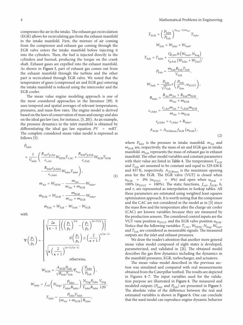1

5

8

6

7

3

4

2

Figure 1 Caterpillar testbed 3126 Sussex University

the observability of the augmented model is well discussedRecently an automated model-based and data-driven designmethodology for automotive engine fault detection andisolation (FDI) is proposed in [15] This methodology whichcombines model-based sequential residual generation anddata-driven statistical residual evaluation is used to create acomplete FDI system for an automotive diesel engine

The problem of designing unknown input observers(UIO) has received great attention in literatureThis problemis motivated by certain applications such as fault diagnosisand control system design If this issue in linear case is wellsolved it remains an open problem in the nonlinear caseThefirst unknown input observers dedicated to linear systemswere proposed in [16 17] Necessary and sufficient conditionsof the existence of the UIO have been well established Newsufficient conditions formulated in terms of linear matrixinequality (LMI) were given by [18]This result is extended in[12] to cover a wide class of nonlinear systems that cannot betreated by the previous approach as well as nonlinear systemswith a large Lipschitz constant

Our aim is to address the issue of actuator fault detectionand isolation for diesel engines Indeed actuators (EGR andVGT) fault diagnosis is necessary and crucial to guaranteeits healthy operation In this work a fault detection andisolation (FDI) system is developed The proposed FDIsystem is composed of two parts residual generation anddecision system Amultiobserver strategy is used for residualgeneration A mean model of diesel engine is exploited forthe design of a set of nonlinear unknown input observersThese observers are designed in order to estimate the statesbehavior without any knowledge of the unknown inputsThesufficient conditions of the existence of the NUIO are givenin terms of linear matrix inequalities (LMIs) The advantageof thismethod is that no a priori assumption on the unknowninput is required and also can be employed for a wider classof nonlinear systems To achieve fault detection and isolation

a decision system based on a statistical approach multi-CUSUM (cumulative sum) is used to process the resultingset of residuals

This paper is organized as follows The experimentalsetup is described in Section 2 The diesel engine modeland its validation are described in Section 3 A nonlinearunknown input observer is presented in Section 4 Section 5describes the residual generation system while the decisionsystem is presented in Section 6The experimental results anddiscussion are presented in Section 7 Finally conclusion andfuture works are given in the last section

The notations used in this paper are quite standard LetRdenote the set of real numbersThe set of 119901 by 119902 real matricesis denoted as R119901times119902 119860119879 and 119860minus1 represent the transpose of119860 and its left inverse (assuming 119860 has full column rank)respectively 119868119903 represents the identity matrix of dimension 119903(lowast) is used for the blocks induced by symmetry sdot representsthe usual Euclidean normL119903

2denotes the Lebesgue space119891119886119894

denotes the 119894th component of the vector 119891119886

2 Experimental Installation

The testbed is built with a Caterpillar 3126b truck enginecoupled to a SCHORCH dynamometer controlled by CPCadet Software The Caterpillar engine is presented inFigure 1 The front and back view of the testbed are shownby the pictures numbered (1) and (2) respectively Enginersquoscomponents are inlet manifold (3) encoder for measuring ofthe engine speed (4) intake air flowmeter (5) exhaust mani-fold (6) GT3782VA variable geometry turbocharger (7) andexhaust gas valve (8) In order to enable a transient controlof the EGR and VGT a dSPACE MicroAutoBox 14011501real-time controller is connected (see Figure 2) Apart fromthe standard OEM electronic sensors built in for ECU anddynamometer control additional sensors and actuators have



CP Cadet

Control room

MatlabSimulink and

Sens

ors s

igna

l

Actu

ator

s sig

nal

Sensors signal

Actuators signal

dSPACE MicroAutoBox


Data recording

ControlDeskreg








Intercooler

Compressor

Air flow meter

AFR sensor

VGT

Inlet manifold

Pressure sensor

Cylinders

Crankshaft

EGR gas cooler

EGR

Pressure sensor

Exhaust manifold








Inlet

=1

119881Inlet(119877Air119888119901Air

119888VAir119882HFM119879CAC +

119877Exh119888119901Exh

119888VExh119882EGR119879EGR




119898Air + 119898EGR119882Inlet


119898Air + 119898EGR119882Inlet


(1)

with

Ψ(1199011

1199010) =

radic2120581

120581 minus 1((

1199011

1199010)

2120581

minus (1199011

1199010)

(120581+1)120581

)

if(1199011

1199010) ge (

2

120581 + 1)

120581(120581minus1)

radic120581(2

120581 + 1)

(120581+1)(120581minus1)

otherwise

119882EGR =119860EGR119875Exh


(119875Inlet119875Exh

)




119881Eng

120


(119898Air + 119898EGR) 119877Inlet

119879EGR = (119875Inlet119875Exh

)


119879Exh

119882Exh = 119882Inlet +119882Fuel


119888119901Exh (119882Inlet +119882Fuel)

119875Exh =119898Exh119877Exh119879Exh

119881Exh

119882Turb =119875Exh

radic119879Exh120591 (

119875Exh119875Atm

119906XVNT)


119898Air + 119898EGR


119898Air + 119898EGR



(2)






0

EGR

posit

ion

()

5 10 15 20 25 3015

20

25

30

35

40

45

(a)

0 5 10 15 20 25 3025

VGT

posit

ion

()

30

35

40

45

50

55

(b)

0 5 10 15 20 25 301400

1450

1500

1550

1600

1650

1700

1750

1800

1850

1900

Engi

ne sp

eed

(min

minus1)

(c)


0 5 10 15 20 25 3012

14

16

18

2

22

24

26

28

3times105

PIn

let

(Pa)

(a)

0 5 10 15 20 25 301

15

2

25

3

35times105

PEx

h(P

a)

(b)



0

Inle

t pre

ssur

e err

or

5 10 15 20 25 300

05

1

15

2

25

3

35

4

45

5times104

(a)

0 5 10 15 20 25 300

05

1

15

2

25

3

35

4

45

5times104

Exha

ust p

ress

ure e

rror

(b)


0 5 10 15 20 25 301

15

2

25

3

35

4

45

5

55times10minus3

mA

ir(k

g)

(a)

0 5 10 15 20 25 300

05

1

15

2

25

3

35times10minus4

mEG

R(k

g)

(b)







=

119899120588

sum

119895=1

120588119895119860119895119909 + 119861119892119892 (120592 119910 119906) + 119891 (119909 119906) + 119861119891119891119886 + 119861119908119908

(3a)

119910 = 119862119909 + 119863119908119908 (3b)





119899120588

sum

119895=1

120588119895 = 1 120588119895 ge 0 forall119895 isin 1 119899120588 (4)


119861119891119891119886 =

119899119891119886

sum

119894=1

119861119891119894119891119886119894 (5)



=

119899120588

sum

119895=1

120588119895119860119895119909 + 119861119892119892 (120592 119910 119906) + 119891 (119909 119906) + 119861119889119889 + 119861119908119908 (6a)

119910 = 119862119909 + 119863119908119908 (6b)

where 119861119889 = 119861119891119894 119861119908 = [119861119908 119861119891] 119863119908 = [119863119908 0] and119908 = [

119908

119891119886





= 119873 (120588) 119911 + 119866119892 (120592 119910 119906) + 119872119891 (119909 119906) + 119871 (120588) 119910 (7a)

119909 = 119911 minus 119864119910 (7b)

119903 = Π119903 (119910 minus 119862119909) (7c)

with119873(120588) = sum119899120588

119895=1120588119895119873119895 and 119871(120588) = sum

119899120588

119895=1120588119895119871119895 Π119903 is a known



119890 = 119873119890 + (119866 minus119872119861119892) 119892 (120592 119910 119906) + (119873119872 + 119871119862 minus119872119860) 119909


(8)



119871 (120588) = 119870 (120588) times (119868 + 119862119864) minus119872119860(120588) 119864 (9b)

119866 = 119872119861119892 (9c)

119872 = 119868 + 119864119862 (9d)

119872119861119889 = 0 (9e)



119864 = 119880 + 119884119881 (10)




119879119883)

minus1119883119879






lim119905rarrinfin

119890 (119905) = 0 for 119908 (119905) = 0 (12a)

119890L1198991199092

le 120574 119908119903

12for 119908 (119905) = 0 119890 (0) = 0 (12b)

where sdot 119903119896119901



Γ = Υ + 119890119879119890 minus 120574

2119908119879119908 minus 120574

2119879 lt 0 (13)



Γ = 119890119879((119872119860 minus 119870119862)

119879119875 + 119875 (119872119860 minus 119870119862)) 119890

+ 119890119879119875119872119891 + (119872119891)

119879

119875119890

+ 119890119879119875 (119870119863119908 minus119872119861119908) 119908 + 119908

119879(119870119863119908 minus119872119861119908)

119879119875119890

minus 119890119879119875119864119863119908

minus 119879(119864119863119908)

119879119875119890 + 119890

119879119890 minus 120574

2119908119879119908 minus 120574

2119879

(14)



119864119904

=

119890119904 (119894) | 119890119904 (119894) = (0 0

119894119905ℎ⏞⏞⏞⏞⏞⏞⏞1 0 0⏟⏟⏟⏟⏟⏟⏟⏟⏟⏟⏟⏟⏟⏟⏟⏟⏟⏟⏟⏟⏟⏟⏟⏟⏟⏟⏟⏟⏟⏟⏟⏟⏟⏟⏟⏟⏟⏟⏟

119904 119888119900119898119901119900119899119890119899119905119904

)

119879

119894 = 1 sdot sdot sdot 119904

(15)



119894119895and 120575min



119891 (1199042) minus 119891 (1199041)

= [

[

(

119899119899

sum

119894119895=1

119867max119894119895

120575max119894119895) + (

119899119899

sum

119894119895=1

119867min119894119895120575min119894119895)]

]

(1199042 minus 1199041)

120575max119894119895 120575

min119894119895

ge 0 120575max119894119895

+ 120575min119894119895

= 1

(16)

where

(i) ℎmax119894119895

ge max(120597119891119894120597119909119895) and ℎmin119894119895

le min(120597119891119894120597119909119895)

(ii) 119867max119894119895

= 119890119899(119894)119890119879

119899(119895)ℎ

max119894119895

and119867min119894119895

= 119890119899(119894)119890119879

119899(119895)ℎ

min119894119895






119875 gt 0 (17a)

[[[

[

Ξmax119894119895119896

Φ119896 minus119875119884119863119908 minus 119884119881119863119908

(lowast) minus120583119868 0


]]]

]

lt 0 (17b)

[[[

[

Ξmin119894119895119896

Φ119896 minus119875119884119863119908 minus 119884119881119863119908

(lowast) minus120583119868 0


]]]

]

lt 0 (17c)

forall119894 = 1 119899 119895 = 1 119899 and 119896 = 1 119899120588 where

Φ119896 = minus119870119896119863119908 + 119875 (119868 + 119880119862) 119861119908 + 119884119881119862119861119908 120583 = 1205742

Ξmax119894119895119896

= [(119868 + 119880119862) (119860 + 119867max119894119895)]119879

119875

+ 119875 (119868 + 119880119862) (119860 + 119867max119894119895) minus 119862

119879119870119879

119896

minus 119870119896119862 + (119860 + 119867max119894119895)119879

119862119879119881119879119884119879

+ 119884119881119862 (119860 + 119867max119894119895) + 119868

Ξmin119894119895119896

= [(119868 + 119880119862) (119860 + 119867min119894119895)]

119879

119875

+ 119875 (119868 + 119880119862) (119860 + 119867min119894119895) minus 119862

119879119870119879

119896

minus 119870119896119862 + (119860 + 119867min119894119895)119879

119862119879119881119879119884119879

+ 119884119881119862(119860 + 119867min119894119895) + 119868

119867max119894119895

= 119885119867119867max119894119895

119867min119894119895

= 119885119867119867min119894119895

(18)






119894119895=1(120575

max119894119895

+ 120575min119894119895) is less than 1


119885119867 =

119899119899

sum

119894119895=1

(120575max119894119895

+ 120575min119894119895) = 119899 times 119899 minus 1198990

sum119899119899

119894119895=1(120575

max119894119895

+ 120575min119894119895)

119885119867

= 1

(19)



Residual generation

System

Diesel engine

NUIO 1

NUIO 2

Decisionsystem

Diagnosis result

Actuator FDI system

yoplus

oplus

uEGR

uXVNT

fa1

fa2

120592120588

120592120588

120592120588

r1

r2

r

Figure 8 FDI system












119879

(20)


119861119889 = [0 0 0 1]119879 (21)


119903 1198911 1198912

1199031 0 times

1199032 times 0



1015840

1(119905) 119903

1015840

2(119905)]


119903 (119896) = 1199030 (119896) +

2

sum

ℓ=1

]ℓΓℓ (119896) 1119896ge1198960120575ℓ (22)










6 Decision System


H0 L (119903 (119894)) =N (1205830 Σ) 119894 = 1 119896

Hℓ L (119903 (119894)) =N (1205830 Σ) 119894 = 1 1198960 minus 1

L (119903 (119894)) =N (120583ℓ Σ) 119894 = 1198960 119896

(23)


119904119896 (ℓ 0) = ln119901ℓ (119903 (119896))

1199010 (119903 (119896)) (24)



1

2(120583

ℓ+ 120583

0)) (25)


119892119896 (ℓ 0) = max (0 119892119896minus1 (ℓ 0) + 119904119896 (ℓ 0)) (26)




119892ℓ= min




ℎℓ119895 =

ℎℓ119889 for 119895 = 0

ℎℓ119894 for 1 le 119895 = ℓ le 119899119891(28)


120591 = max(ℎℓ119889

120581ℓ0

ℎℓ119894



120581ℓ119895 =1

2(120583

ℓminus 120583

119895)119879

Σminus1(120583

ℓminus 120583

119895) (30)















minus3m3



119892lowast

ℓ= min

0le119895 =ℓle2(119892119896 (ℓ 0) minus 119892119896 (119895 0)) (31)







minus3 s




002040608

1

002040608

1

0 2 4 6 8 10 12 14

0 2 4 6 8 10 12 14

uEG

Ru

XVG

T

(a)

4 6 8 10 12 14

4 6 8 10 12 14

0

1

2

minus1

minus2

0

1

2

minus1

minus2

r 1r 2

(b)

0

100

200

300

4 6 8 10 12 14

4 6 8 10 12 14

0

100

200

300

glowast 2

glowast 1

(c)











11991110 = [12 0 2 times 10minus7

10minus10]119879

11991120 = [12 0 2 times 10minus7

10minus10]119879

(32)


lowast




8 Conclusion


Appendices


See Table 3

B Nomenclature

See Table 4



119909 = [119875Inlet 119898Air 119898EGR 119898Exh]119879

119906 = [119906EGR 119906XVNT]119879

119910 = [119875Inlet 119875Exh]119879

120588 = 119873Eng

120592 = [119879CAC 119882HFM 119882Fuel]119879

(C1)


1198601

=

[[[[[[[[[[[[[[

[


120119881Inlet0 0 0


120119881Inlet0 0

0 0 minus119891vol119873Eng119881Eng

120119881Inlet0

0119891vol119873Eng119881Eng

120119881Inlet

119891vol119873Eng119881Eng

120119881Inlet0

]]]]]]]]]]]]]]

]

1198602

=

[[[[[[[[[[[[[[

[


120119881Inlet0 0 0


120119881Inlet0 0

0 0 minus119891vol119873Eng119881Eng

120119881Inlet0

0119891vol119873Eng119881Eng

120119881Inlet

119891vol119873Eng119881Eng

120119881Inlet0

]]]]]]]]]]]]]]

]

(C2)


1205881 =119873Eng minus 119873Eng

119873Eng minus 119873Eng 1205882 =




119861119892 =

[[[[[

[

119877Air119888119901Air

119888VAir119881Inlet0 0

0 1 0

0 0 0

0 0 1

]]]]]

]

119862 =[[

[

1 0 0 0

0 0 0119877Exh119879

moyExh

119881Exh

]]

]

119861119908 = [0 0 0 0]119879

(C4)



119861119891 =

[[[[[[

[



0 0

119860EGRmax 0

minus119860EGRmax 1

]]]]]]

]

119891119886 =

[[[[

[

119875Exh


(119875Inlet119875Exh

)119891EGR (119906EGR)

119875Exh

radic119879Exh120591 (

119875Exh119875Atm

119906XVNT)

]]]]

]

(C5)


119892 = [119882HFM119879CAC 119882HFM 119882Fuel]119879 (C6)

119891 =

[[[[[[[[[[[

[


119860EGR119898ExhΨ120581Exh119879Exh




]]]]]]]]]]]

]

(C7)





Acknowledgments


References






































Volume 2014




Journal of











Journal of


Function Spaces






Algebra











CP Cadet

Control room

MatlabSimulink and

Sens

ors s

igna

l

Actu

ator

s sig

nal

Sensors signal

Actuators signal

dSPACE MicroAutoBox


Data recording

ControlDeskreg








Intercooler

Compressor

Air flow meter

AFR sensor

VGT

Inlet manifold

Pressure sensor

Cylinders

Crankshaft

EGR gas cooler

EGR

Pressure sensor

Exhaust manifold








Inlet

=1

119881Inlet(119877Air119888119901Air

119888VAir119882HFM119879CAC +

119877Exh119888119901Exh

119888VExh119882EGR119879EGR




119898Air + 119898EGR119882Inlet


119898Air + 119898EGR119882Inlet


(1)

with

Ψ(1199011

1199010) =

radic2120581

120581 minus 1((

1199011

1199010)

2120581

minus (1199011

1199010)

(120581+1)120581

)

if(1199011

1199010) ge (

2

120581 + 1)

120581(120581minus1)

radic120581(2

120581 + 1)

(120581+1)(120581minus1)

otherwise

119882EGR =119860EGR119875Exh


(119875Inlet119875Exh

)




119881Eng

120


(119898Air + 119898EGR) 119877Inlet

119879EGR = (119875Inlet119875Exh

)


119879Exh

119882Exh = 119882Inlet +119882Fuel


119888119901Exh (119882Inlet +119882Fuel)

119875Exh =119898Exh119877Exh119879Exh

119881Exh

119882Turb =119875Exh

radic119879Exh120591 (

119875Exh119875Atm

119906XVNT)


119898Air + 119898EGR


119898Air + 119898EGR



(2)






0

EGR

posit

ion

()

5 10 15 20 25 3015

20

25

30

35

40

45

(a)

0 5 10 15 20 25 3025

VGT

posit

ion

()

30

35

40

45

50

55

(b)

0 5 10 15 20 25 301400

1450

1500

1550

1600

1650

1700

1750

1800

1850

1900

Engi

ne sp

eed

(min

minus1)

(c)


0 5 10 15 20 25 3012

14

16

18

2

22

24

26

28

3times105

PIn

let

(Pa)

(a)

0 5 10 15 20 25 301

15

2

25

3

35times105

PEx

h(P

a)

(b)



0

Inle

t pre

ssur

e err

or

5 10 15 20 25 300

05

1

15

2

25

3

35

4

45

5times104

(a)

0 5 10 15 20 25 300

05

1

15

2

25

3

35

4

45

5times104

Exha

ust p

ress

ure e

rror

(b)


0 5 10 15 20 25 301

15

2

25

3

35

4

45

5

55times10minus3

mA

ir(k

g)

(a)

0 5 10 15 20 25 300

05

1

15

2

25

3

35times10minus4

mEG

R(k

g)

(b)







=

119899120588

sum

119895=1

120588119895119860119895119909 + 119861119892119892 (120592 119910 119906) + 119891 (119909 119906) + 119861119891119891119886 + 119861119908119908

(3a)

119910 = 119862119909 + 119863119908119908 (3b)





119899120588

sum

119895=1

120588119895 = 1 120588119895 ge 0 forall119895 isin 1 119899120588 (4)


119861119891119891119886 =

119899119891119886

sum

119894=1

119861119891119894119891119886119894 (5)



=

119899120588

sum

119895=1

120588119895119860119895119909 + 119861119892119892 (120592 119910 119906) + 119891 (119909 119906) + 119861119889119889 + 119861119908119908 (6a)

119910 = 119862119909 + 119863119908119908 (6b)

where 119861119889 = 119861119891119894 119861119908 = [119861119908 119861119891] 119863119908 = [119863119908 0] and119908 = [

119908

119891119886





= 119873 (120588) 119911 + 119866119892 (120592 119910 119906) + 119872119891 (119909 119906) + 119871 (120588) 119910 (7a)

119909 = 119911 minus 119864119910 (7b)

119903 = Π119903 (119910 minus 119862119909) (7c)

with119873(120588) = sum119899120588

119895=1120588119895119873119895 and 119871(120588) = sum

119899120588

119895=1120588119895119871119895 Π119903 is a known



119890 = 119873119890 + (119866 minus119872119861119892) 119892 (120592 119910 119906) + (119873119872 + 119871119862 minus119872119860) 119909


(8)



119871 (120588) = 119870 (120588) times (119868 + 119862119864) minus119872119860(120588) 119864 (9b)

119866 = 119872119861119892 (9c)

119872 = 119868 + 119864119862 (9d)

119872119861119889 = 0 (9e)



119864 = 119880 + 119884119881 (10)




119879119883)

minus1119883119879






lim119905rarrinfin

119890 (119905) = 0 for 119908 (119905) = 0 (12a)

119890L1198991199092

le 120574 119908119903

12for 119908 (119905) = 0 119890 (0) = 0 (12b)

where sdot 119903119896119901



Γ = Υ + 119890119879119890 minus 120574

2119908119879119908 minus 120574

2119879 lt 0 (13)



Γ = 119890119879((119872119860 minus 119870119862)

119879119875 + 119875 (119872119860 minus 119870119862)) 119890

+ 119890119879119875119872119891 + (119872119891)

119879

119875119890

+ 119890119879119875 (119870119863119908 minus119872119861119908) 119908 + 119908

119879(119870119863119908 minus119872119861119908)

119879119875119890

minus 119890119879119875119864119863119908

minus 119879(119864119863119908)

119879119875119890 + 119890

119879119890 minus 120574

2119908119879119908 minus 120574

2119879

(14)



119864119904

=

119890119904 (119894) | 119890119904 (119894) = (0 0

119894119905ℎ⏞⏞⏞⏞⏞⏞⏞1 0 0⏟⏟⏟⏟⏟⏟⏟⏟⏟⏟⏟⏟⏟⏟⏟⏟⏟⏟⏟⏟⏟⏟⏟⏟⏟⏟⏟⏟⏟⏟⏟⏟⏟⏟⏟⏟⏟⏟⏟

119904 119888119900119898119901119900119899119890119899119905119904

)

119879

119894 = 1 sdot sdot sdot 119904

(15)



119894119895and 120575min



119891 (1199042) minus 119891 (1199041)

= [

[

(

119899119899

sum

119894119895=1

119867max119894119895

120575max119894119895) + (

119899119899

sum

119894119895=1

119867min119894119895120575min119894119895)]

]

(1199042 minus 1199041)

120575max119894119895 120575

min119894119895

ge 0 120575max119894119895

+ 120575min119894119895

= 1

(16)

where

(i) ℎmax119894119895

ge max(120597119891119894120597119909119895) and ℎmin119894119895

le min(120597119891119894120597119909119895)

(ii) 119867max119894119895

= 119890119899(119894)119890119879

119899(119895)ℎ

max119894119895

and119867min119894119895

= 119890119899(119894)119890119879

119899(119895)ℎ

min119894119895






119875 gt 0 (17a)

[[[

[

Ξmax119894119895119896

Φ119896 minus119875119884119863119908 minus 119884119881119863119908

(lowast) minus120583119868 0


]]]

]

lt 0 (17b)

[[[

[

Ξmin119894119895119896

Φ119896 minus119875119884119863119908 minus 119884119881119863119908

(lowast) minus120583119868 0


]]]

]

lt 0 (17c)

forall119894 = 1 119899 119895 = 1 119899 and 119896 = 1 119899120588 where

Φ119896 = minus119870119896119863119908 + 119875 (119868 + 119880119862) 119861119908 + 119884119881119862119861119908 120583 = 1205742

Ξmax119894119895119896

= [(119868 + 119880119862) (119860 + 119867max119894119895)]119879

119875

+ 119875 (119868 + 119880119862) (119860 + 119867max119894119895) minus 119862

119879119870119879

119896

minus 119870119896119862 + (119860 + 119867max119894119895)119879

119862119879119881119879119884119879

+ 119884119881119862 (119860 + 119867max119894119895) + 119868

Ξmin119894119895119896

= [(119868 + 119880119862) (119860 + 119867min119894119895)]

119879

119875

+ 119875 (119868 + 119880119862) (119860 + 119867min119894119895) minus 119862

119879119870119879

119896

minus 119870119896119862 + (119860 + 119867min119894119895)119879

119862119879119881119879119884119879

+ 119884119881119862(119860 + 119867min119894119895) + 119868

119867max119894119895

= 119885119867119867max119894119895

119867min119894119895

= 119885119867119867min119894119895

(18)






119894119895=1(120575

max119894119895

+ 120575min119894119895) is less than 1


119885119867 =

119899119899

sum

119894119895=1

(120575max119894119895

+ 120575min119894119895) = 119899 times 119899 minus 1198990

sum119899119899

119894119895=1(120575

max119894119895

+ 120575min119894119895)

119885119867

= 1

(19)



Residual generation

System

Diesel engine

NUIO 1

NUIO 2

Decisionsystem

Diagnosis result

Actuator FDI system

yoplus

oplus

uEGR

uXVNT

fa1

fa2

120592120588

120592120588

120592120588

r1

r2

r

Figure 8 FDI system












119879

(20)


119861119889 = [0 0 0 1]119879 (21)


119903 1198911 1198912

1199031 0 times

1199032 times 0



1015840

1(119905) 119903

1015840

2(119905)]


119903 (119896) = 1199030 (119896) +

2

sum

ℓ=1

]ℓΓℓ (119896) 1119896ge1198960120575ℓ (22)










6 Decision System


H0 L (119903 (119894)) =N (1205830 Σ) 119894 = 1 119896

Hℓ L (119903 (119894)) =N (1205830 Σ) 119894 = 1 1198960 minus 1

L (119903 (119894)) =N (120583ℓ Σ) 119894 = 1198960 119896

(23)


119904119896 (ℓ 0) = ln119901ℓ (119903 (119896))

1199010 (119903 (119896)) (24)



1

2(120583

ℓ+ 120583

0)) (25)


119892119896 (ℓ 0) = max (0 119892119896minus1 (ℓ 0) + 119904119896 (ℓ 0)) (26)




119892ℓ= min




ℎℓ119895 =

ℎℓ119889 for 119895 = 0

ℎℓ119894 for 1 le 119895 = ℓ le 119899119891(28)


120591 = max(ℎℓ119889

120581ℓ0

ℎℓ119894



120581ℓ119895 =1

2(120583

ℓminus 120583

119895)119879

Σminus1(120583

ℓminus 120583

119895) (30)















minus3m3



119892lowast

ℓ= min

0le119895 =ℓle2(119892119896 (ℓ 0) minus 119892119896 (119895 0)) (31)







minus3 s




002040608

1

002040608

1

0 2 4 6 8 10 12 14

0 2 4 6 8 10 12 14

uEG

Ru

XVG

T

(a)

4 6 8 10 12 14

4 6 8 10 12 14

0

1

2

minus1

minus2

0

1

2

minus1

minus2

r 1r 2

(b)

0

100

200

300

4 6 8 10 12 14

4 6 8 10 12 14

0

100

200

300

glowast 2

glowast 1

(c)











11991110 = [12 0 2 times 10minus7

10minus10]119879

11991120 = [12 0 2 times 10minus7

10minus10]119879

(32)


lowast




8 Conclusion


Appendices


See Table 3

B Nomenclature

See Table 4



119909 = [119875Inlet 119898Air 119898EGR 119898Exh]119879

119906 = [119906EGR 119906XVNT]119879

119910 = [119875Inlet 119875Exh]119879

120588 = 119873Eng

120592 = [119879CAC 119882HFM 119882Fuel]119879

(C1)


1198601

=

[[[[[[[[[[[[[[

[


120119881Inlet0 0 0


120119881Inlet0 0

0 0 minus119891vol119873Eng119881Eng

120119881Inlet0

0119891vol119873Eng119881Eng

120119881Inlet

119891vol119873Eng119881Eng

120119881Inlet0

]]]]]]]]]]]]]]

]

1198602

=

[[[[[[[[[[[[[[

[


120119881Inlet0 0 0


120119881Inlet0 0

0 0 minus119891vol119873Eng119881Eng

120119881Inlet0

0119891vol119873Eng119881Eng

120119881Inlet

119891vol119873Eng119881Eng

120119881Inlet0

]]]]]]]]]]]]]]

]

(C2)


1205881 =119873Eng minus 119873Eng

119873Eng minus 119873Eng 1205882 =




119861119892 =

[[[[[

[

119877Air119888119901Air

119888VAir119881Inlet0 0

0 1 0

0 0 0

0 0 1

]]]]]

]

119862 =[[

[

1 0 0 0

0 0 0119877Exh119879

moyExh

119881Exh

]]

]

119861119908 = [0 0 0 0]119879

(C4)



119861119891 =

[[[[[[

[



0 0

119860EGRmax 0

minus119860EGRmax 1

]]]]]]

]

119891119886 =

[[[[

[

119875Exh


(119875Inlet119875Exh

)119891EGR (119906EGR)

119875Exh

radic119879Exh120591 (

119875Exh119875Atm

119906XVNT)

]]]]

]

(C5)


119892 = [119882HFM119879CAC 119882HFM 119882Fuel]119879 (C6)

119891 =

[[[[[[[[[[[

[


119860EGR119898ExhΨ120581Exh119879Exh




]]]]]]]]]]]

]

(C7)





Acknowledgments


References






































Volume 2014




Journal of











Journal of


Function Spaces






Algebra












Inlet

=1

119881Inlet(119877Air119888119901Air

119888VAir119882HFM119879CAC +

119877Exh119888119901Exh

119888VExh119882EGR119879EGR




119898Air + 119898EGR119882Inlet


119898Air + 119898EGR119882Inlet


(1)

with

Ψ(1199011

1199010) =

radic2120581

120581 minus 1((

1199011

1199010)

2120581

minus (1199011

1199010)

(120581+1)120581

)

if(1199011

1199010) ge (

2

120581 + 1)

120581(120581minus1)

radic120581(2

120581 + 1)

(120581+1)(120581minus1)

otherwise

119882EGR =119860EGR119875Exh


(119875Inlet119875Exh

)




119881Eng

120


(119898Air + 119898EGR) 119877Inlet

119879EGR = (119875Inlet119875Exh

)


119879Exh

119882Exh = 119882Inlet +119882Fuel


119888119901Exh (119882Inlet +119882Fuel)

119875Exh =119898Exh119877Exh119879Exh

119881Exh

119882Turb =119875Exh

radic119879Exh120591 (

119875Exh119875Atm

119906XVNT)


119898Air + 119898EGR


119898Air + 119898EGR



(2)






0

EGR

posit

ion

()

5 10 15 20 25 3015

20

25

30

35

40

45

(a)

0 5 10 15 20 25 3025

VGT

posit

ion

()

30

35

40

45

50

55

(b)

0 5 10 15 20 25 301400

1450

1500

1550

1600

1650

1700

1750

1800

1850

1900

Engi

ne sp

eed

(min

minus1)

(c)


0 5 10 15 20 25 3012

14

16

18

2

22

24

26

28

3times105

PIn

let

(Pa)

(a)

0 5 10 15 20 25 301

15

2

25

3

35times105

PEx

h(P

a)

(b)



0

Inle

t pre

ssur

e err

or

5 10 15 20 25 300

05

1

15

2

25

3

35

4

45

5times104

(a)

0 5 10 15 20 25 300

05

1

15

2

25

3

35

4

45

5times104

Exha

ust p

ress

ure e

rror

(b)


0 5 10 15 20 25 301

15

2

25

3

35

4

45

5

55times10minus3

mA

ir(k

g)

(a)

0 5 10 15 20 25 300

05

1

15

2

25

3

35times10minus4

mEG

R(k

g)

(b)







=

119899120588

sum

119895=1

120588119895119860119895119909 + 119861119892119892 (120592 119910 119906) + 119891 (119909 119906) + 119861119891119891119886 + 119861119908119908

(3a)

119910 = 119862119909 + 119863119908119908 (3b)





119899120588

sum

119895=1

120588119895 = 1 120588119895 ge 0 forall119895 isin 1 119899120588 (4)


119861119891119891119886 =

119899119891119886

sum

119894=1

119861119891119894119891119886119894 (5)



=

119899120588

sum

119895=1

120588119895119860119895119909 + 119861119892119892 (120592 119910 119906) + 119891 (119909 119906) + 119861119889119889 + 119861119908119908 (6a)

119910 = 119862119909 + 119863119908119908 (6b)

where 119861119889 = 119861119891119894 119861119908 = [119861119908 119861119891] 119863119908 = [119863119908 0] and119908 = [

119908

119891119886





= 119873 (120588) 119911 + 119866119892 (120592 119910 119906) + 119872119891 (119909 119906) + 119871 (120588) 119910 (7a)

119909 = 119911 minus 119864119910 (7b)

119903 = Π119903 (119910 minus 119862119909) (7c)

with119873(120588) = sum119899120588

119895=1120588119895119873119895 and 119871(120588) = sum

119899120588

119895=1120588119895119871119895 Π119903 is a known



119890 = 119873119890 + (119866 minus119872119861119892) 119892 (120592 119910 119906) + (119873119872 + 119871119862 minus119872119860) 119909


(8)



119871 (120588) = 119870 (120588) times (119868 + 119862119864) minus119872119860(120588) 119864 (9b)

119866 = 119872119861119892 (9c)

119872 = 119868 + 119864119862 (9d)

119872119861119889 = 0 (9e)



119864 = 119880 + 119884119881 (10)




119879119883)

minus1119883119879






lim119905rarrinfin

119890 (119905) = 0 for 119908 (119905) = 0 (12a)

119890L1198991199092

le 120574 119908119903

12for 119908 (119905) = 0 119890 (0) = 0 (12b)

where sdot 119903119896119901



Γ = Υ + 119890119879119890 minus 120574

2119908119879119908 minus 120574

2119879 lt 0 (13)



Γ = 119890119879((119872119860 minus 119870119862)

119879119875 + 119875 (119872119860 minus 119870119862)) 119890

+ 119890119879119875119872119891 + (119872119891)

119879

119875119890

+ 119890119879119875 (119870119863119908 minus119872119861119908) 119908 + 119908

119879(119870119863119908 minus119872119861119908)

119879119875119890

minus 119890119879119875119864119863119908

minus 119879(119864119863119908)

119879119875119890 + 119890

119879119890 minus 120574

2119908119879119908 minus 120574

2119879

(14)



119864119904

=

119890119904 (119894) | 119890119904 (119894) = (0 0

119894119905ℎ⏞⏞⏞⏞⏞⏞⏞1 0 0⏟⏟⏟⏟⏟⏟⏟⏟⏟⏟⏟⏟⏟⏟⏟⏟⏟⏟⏟⏟⏟⏟⏟⏟⏟⏟⏟⏟⏟⏟⏟⏟⏟⏟⏟⏟⏟⏟⏟

119904 119888119900119898119901119900119899119890119899119905119904

)

119879

119894 = 1 sdot sdot sdot 119904

(15)



119894119895and 120575min



119891 (1199042) minus 119891 (1199041)

= [

[

(

119899119899

sum

119894119895=1

119867max119894119895

120575max119894119895) + (

119899119899

sum

119894119895=1

119867min119894119895120575min119894119895)]

]

(1199042 minus 1199041)

120575max119894119895 120575

min119894119895

ge 0 120575max119894119895

+ 120575min119894119895

= 1

(16)

where

(i) ℎmax119894119895

ge max(120597119891119894120597119909119895) and ℎmin119894119895

le min(120597119891119894120597119909119895)

(ii) 119867max119894119895

= 119890119899(119894)119890119879

119899(119895)ℎ

max119894119895

and119867min119894119895

= 119890119899(119894)119890119879

119899(119895)ℎ

min119894119895






119875 gt 0 (17a)

[[[

[

Ξmax119894119895119896

Φ119896 minus119875119884119863119908 minus 119884119881119863119908

(lowast) minus120583119868 0


]]]

]

lt 0 (17b)

[[[

[

Ξmin119894119895119896

Φ119896 minus119875119884119863119908 minus 119884119881119863119908

(lowast) minus120583119868 0


]]]

]

lt 0 (17c)

forall119894 = 1 119899 119895 = 1 119899 and 119896 = 1 119899120588 where

Φ119896 = minus119870119896119863119908 + 119875 (119868 + 119880119862) 119861119908 + 119884119881119862119861119908 120583 = 1205742

Ξmax119894119895119896

= [(119868 + 119880119862) (119860 + 119867max119894119895)]119879

119875

+ 119875 (119868 + 119880119862) (119860 + 119867max119894119895) minus 119862

119879119870119879

119896

minus 119870119896119862 + (119860 + 119867max119894119895)119879

119862119879119881119879119884119879

+ 119884119881119862 (119860 + 119867max119894119895) + 119868

Ξmin119894119895119896

= [(119868 + 119880119862) (119860 + 119867min119894119895)]

119879

119875

+ 119875 (119868 + 119880119862) (119860 + 119867min119894119895) minus 119862

119879119870119879

119896

minus 119870119896119862 + (119860 + 119867min119894119895)119879

119862119879119881119879119884119879

+ 119884119881119862(119860 + 119867min119894119895) + 119868

119867max119894119895

= 119885119867119867max119894119895

119867min119894119895

= 119885119867119867min119894119895

(18)






119894119895=1(120575

max119894119895

+ 120575min119894119895) is less than 1


119885119867 =

119899119899

sum

119894119895=1

(120575max119894119895

+ 120575min119894119895) = 119899 times 119899 minus 1198990

sum119899119899

119894119895=1(120575

max119894119895

+ 120575min119894119895)

119885119867

= 1

(19)



Residual generation

System

Diesel engine

NUIO 1

NUIO 2

Decisionsystem

Diagnosis result

Actuator FDI system

yoplus

oplus

uEGR

uXVNT

fa1

fa2

120592120588

120592120588

120592120588

r1

r2

r

Figure 8 FDI system












119879

(20)


119861119889 = [0 0 0 1]119879 (21)


119903 1198911 1198912

1199031 0 times

1199032 times 0



1015840

1(119905) 119903

1015840

2(119905)]


119903 (119896) = 1199030 (119896) +

2

sum

ℓ=1

]ℓΓℓ (119896) 1119896ge1198960120575ℓ (22)










6 Decision System


H0 L (119903 (119894)) =N (1205830 Σ) 119894 = 1 119896

Hℓ L (119903 (119894)) =N (1205830 Σ) 119894 = 1 1198960 minus 1

L (119903 (119894)) =N (120583ℓ Σ) 119894 = 1198960 119896

(23)


119904119896 (ℓ 0) = ln119901ℓ (119903 (119896))

1199010 (119903 (119896)) (24)



1

2(120583

ℓ+ 120583

0)) (25)


119892119896 (ℓ 0) = max (0 119892119896minus1 (ℓ 0) + 119904119896 (ℓ 0)) (26)




119892ℓ= min




ℎℓ119895 =

ℎℓ119889 for 119895 = 0

ℎℓ119894 for 1 le 119895 = ℓ le 119899119891(28)


120591 = max(ℎℓ119889

120581ℓ0

ℎℓ119894



120581ℓ119895 =1

2(120583

ℓminus 120583

119895)119879

Σminus1(120583

ℓminus 120583

119895) (30)















minus3m3



119892lowast

ℓ= min

0le119895 =ℓle2(119892119896 (ℓ 0) minus 119892119896 (119895 0)) (31)







minus3 s




002040608

1

002040608

1

0 2 4 6 8 10 12 14

0 2 4 6 8 10 12 14

uEG

Ru

XVG

T

(a)

4 6 8 10 12 14

4 6 8 10 12 14

0

1

2

minus1

minus2

0

1

2

minus1

minus2

r 1r 2

(b)

0

100

200

300

4 6 8 10 12 14

4 6 8 10 12 14

0

100

200

300

glowast 2

glowast 1

(c)











11991110 = [12 0 2 times 10minus7

10minus10]119879

11991120 = [12 0 2 times 10minus7

10minus10]119879

(32)


lowast




8 Conclusion


Appendices


See Table 3

B Nomenclature

See Table 4



119909 = [119875Inlet 119898Air 119898EGR 119898Exh]119879

119906 = [119906EGR 119906XVNT]119879

119910 = [119875Inlet 119875Exh]119879

120588 = 119873Eng

120592 = [119879CAC 119882HFM 119882Fuel]119879

(C1)


1198601

=

[[[[[[[[[[[[[[

[


120119881Inlet0 0 0


120119881Inlet0 0

0 0 minus119891vol119873Eng119881Eng

120119881Inlet0

0119891vol119873Eng119881Eng

120119881Inlet

119891vol119873Eng119881Eng

120119881Inlet0

]]]]]]]]]]]]]]

]

1198602

=

[[[[[[[[[[[[[[

[


120119881Inlet0 0 0


120119881Inlet0 0

0 0 minus119891vol119873Eng119881Eng

120119881Inlet0

0119891vol119873Eng119881Eng

120119881Inlet

119891vol119873Eng119881Eng

120119881Inlet0

]]]]]]]]]]]]]]

]

(C2)


1205881 =119873Eng minus 119873Eng

119873Eng minus 119873Eng 1205882 =




119861119892 =

[[[[[

[

119877Air119888119901Air

119888VAir119881Inlet0 0

0 1 0

0 0 0

0 0 1

]]]]]

]

119862 =[[

[

1 0 0 0

0 0 0119877Exh119879

moyExh

119881Exh

]]

]

119861119908 = [0 0 0 0]119879

(C4)



119861119891 =

[[[[[[

[



0 0

119860EGRmax 0

minus119860EGRmax 1

]]]]]]

]

119891119886 =

[[[[

[

119875Exh


(119875Inlet119875Exh

)119891EGR (119906EGR)

119875Exh

radic119879Exh120591 (

119875Exh119875Atm

119906XVNT)

]]]]

]

(C5)


119892 = [119882HFM119879CAC 119882HFM 119882Fuel]119879 (C6)

119891 =

[[[[[[[[[[[

[


119860EGR119898ExhΨ120581Exh119879Exh




]]]]]]]]]]]

]

(C7)





Acknowledgments


References






































Volume 2014




Journal of











Journal of


Function Spaces






Algebra










0

EGR

posit

ion

()

5 10 15 20 25 3015

20

25

30

35

40

45

(a)

0 5 10 15 20 25 3025

VGT

posit

ion

()

30

35

40

45

50

55

(b)

0 5 10 15 20 25 301400

1450

1500

1550

1600

1650

1700

1750

1800

1850

1900

Engi

ne sp

eed

(min

minus1)

(c)


0 5 10 15 20 25 3012

14

16

18

2

22

24

26

28

3times105

PIn

let

(Pa)

(a)

0 5 10 15 20 25 301

15

2

25

3

35times105

PEx

h(P

a)

(b)



0

Inle

t pre

ssur

e err

or

5 10 15 20 25 300

05

1

15

2

25

3

35

4

45

5times104

(a)

0 5 10 15 20 25 300

05

1

15

2

25

3

35

4

45

5times104

Exha

ust p

ress

ure e

rror

(b)


0 5 10 15 20 25 301

15

2

25

3

35

4

45

5

55times10minus3

mA

ir(k

g)

(a)

0 5 10 15 20 25 300

05

1

15

2

25

3

35times10minus4

mEG

R(k

g)

(b)







=

119899120588

sum

119895=1

120588119895119860119895119909 + 119861119892119892 (120592 119910 119906) + 119891 (119909 119906) + 119861119891119891119886 + 119861119908119908

(3a)

119910 = 119862119909 + 119863119908119908 (3b)





119899120588

sum

119895=1

120588119895 = 1 120588119895 ge 0 forall119895 isin 1 119899120588 (4)


119861119891119891119886 =

119899119891119886

sum

119894=1

119861119891119894119891119886119894 (5)



=

119899120588

sum

119895=1

120588119895119860119895119909 + 119861119892119892 (120592 119910 119906) + 119891 (119909 119906) + 119861119889119889 + 119861119908119908 (6a)

119910 = 119862119909 + 119863119908119908 (6b)

where 119861119889 = 119861119891119894 119861119908 = [119861119908 119861119891] 119863119908 = [119863119908 0] and119908 = [

119908

119891119886





= 119873 (120588) 119911 + 119866119892 (120592 119910 119906) + 119872119891 (119909 119906) + 119871 (120588) 119910 (7a)

119909 = 119911 minus 119864119910 (7b)

119903 = Π119903 (119910 minus 119862119909) (7c)

with119873(120588) = sum119899120588

119895=1120588119895119873119895 and 119871(120588) = sum

119899120588

119895=1120588119895119871119895 Π119903 is a known



119890 = 119873119890 + (119866 minus119872119861119892) 119892 (120592 119910 119906) + (119873119872 + 119871119862 minus119872119860) 119909


(8)



119871 (120588) = 119870 (120588) times (119868 + 119862119864) minus119872119860(120588) 119864 (9b)

119866 = 119872119861119892 (9c)

119872 = 119868 + 119864119862 (9d)

119872119861119889 = 0 (9e)



119864 = 119880 + 119884119881 (10)




119879119883)

minus1119883119879






lim119905rarrinfin

119890 (119905) = 0 for 119908 (119905) = 0 (12a)

119890L1198991199092

le 120574 119908119903

12for 119908 (119905) = 0 119890 (0) = 0 (12b)

where sdot 119903119896119901



Γ = Υ + 119890119879119890 minus 120574

2119908119879119908 minus 120574

2119879 lt 0 (13)



Γ = 119890119879((119872119860 minus 119870119862)

119879119875 + 119875 (119872119860 minus 119870119862)) 119890

+ 119890119879119875119872119891 + (119872119891)

119879

119875119890

+ 119890119879119875 (119870119863119908 minus119872119861119908) 119908 + 119908

119879(119870119863119908 minus119872119861119908)

119879119875119890

minus 119890119879119875119864119863119908

minus 119879(119864119863119908)

119879119875119890 + 119890

119879119890 minus 120574

2119908119879119908 minus 120574

2119879

(14)



119864119904

=

119890119904 (119894) | 119890119904 (119894) = (0 0

119894119905ℎ⏞⏞⏞⏞⏞⏞⏞1 0 0⏟⏟⏟⏟⏟⏟⏟⏟⏟⏟⏟⏟⏟⏟⏟⏟⏟⏟⏟⏟⏟⏟⏟⏟⏟⏟⏟⏟⏟⏟⏟⏟⏟⏟⏟⏟⏟⏟⏟

119904 119888119900119898119901119900119899119890119899119905119904

)

119879

119894 = 1 sdot sdot sdot 119904

(15)



119894119895and 120575min



119891 (1199042) minus 119891 (1199041)

= [

[

(

119899119899

sum

119894119895=1

119867max119894119895

120575max119894119895) + (

119899119899

sum

119894119895=1

119867min119894119895120575min119894119895)]

]

(1199042 minus 1199041)

120575max119894119895 120575

min119894119895

ge 0 120575max119894119895

+ 120575min119894119895

= 1

(16)

where

(i) ℎmax119894119895

ge max(120597119891119894120597119909119895) and ℎmin119894119895

le min(120597119891119894120597119909119895)

(ii) 119867max119894119895

= 119890119899(119894)119890119879

119899(119895)ℎ

max119894119895

and119867min119894119895

= 119890119899(119894)119890119879

119899(119895)ℎ

min119894119895






119875 gt 0 (17a)

[[[

[

Ξmax119894119895119896

Φ119896 minus119875119884119863119908 minus 119884119881119863119908

(lowast) minus120583119868 0


]]]

]

lt 0 (17b)

[[[

[

Ξmin119894119895119896

Φ119896 minus119875119884119863119908 minus 119884119881119863119908

(lowast) minus120583119868 0


]]]

]

lt 0 (17c)

forall119894 = 1 119899 119895 = 1 119899 and 119896 = 1 119899120588 where

Φ119896 = minus119870119896119863119908 + 119875 (119868 + 119880119862) 119861119908 + 119884119881119862119861119908 120583 = 1205742

Ξmax119894119895119896

= [(119868 + 119880119862) (119860 + 119867max119894119895)]119879

119875

+ 119875 (119868 + 119880119862) (119860 + 119867max119894119895) minus 119862

119879119870119879

119896

minus 119870119896119862 + (119860 + 119867max119894119895)119879

119862119879119881119879119884119879

+ 119884119881119862 (119860 + 119867max119894119895) + 119868

Ξmin119894119895119896

= [(119868 + 119880119862) (119860 + 119867min119894119895)]

119879

119875

+ 119875 (119868 + 119880119862) (119860 + 119867min119894119895) minus 119862

119879119870119879

119896

minus 119870119896119862 + (119860 + 119867min119894119895)119879

119862119879119881119879119884119879

+ 119884119881119862(119860 + 119867min119894119895) + 119868

119867max119894119895

= 119885119867119867max119894119895

119867min119894119895

= 119885119867119867min119894119895

(18)






119894119895=1(120575

max119894119895

+ 120575min119894119895) is less than 1


119885119867 =

119899119899

sum

119894119895=1

(120575max119894119895

+ 120575min119894119895) = 119899 times 119899 minus 1198990

sum119899119899

119894119895=1(120575

max119894119895

+ 120575min119894119895)

119885119867

= 1

(19)



Residual generation

System

Diesel engine

NUIO 1

NUIO 2

Decisionsystem

Diagnosis result

Actuator FDI system

yoplus

oplus

uEGR

uXVNT

fa1

fa2

120592120588

120592120588

120592120588

r1

r2

r

Figure 8 FDI system












119879

(20)


119861119889 = [0 0 0 1]119879 (21)


119903 1198911 1198912

1199031 0 times

1199032 times 0



1015840

1(119905) 119903

1015840

2(119905)]


119903 (119896) = 1199030 (119896) +

2

sum

ℓ=1

]ℓΓℓ (119896) 1119896ge1198960120575ℓ (22)










6 Decision System


H0 L (119903 (119894)) =N (1205830 Σ) 119894 = 1 119896

Hℓ L (119903 (119894)) =N (1205830 Σ) 119894 = 1 1198960 minus 1

L (119903 (119894)) =N (120583ℓ Σ) 119894 = 1198960 119896

(23)


119904119896 (ℓ 0) = ln119901ℓ (119903 (119896))

1199010 (119903 (119896)) (24)



1

2(120583

ℓ+ 120583

0)) (25)


119892119896 (ℓ 0) = max (0 119892119896minus1 (ℓ 0) + 119904119896 (ℓ 0)) (26)




119892ℓ= min




ℎℓ119895 =

ℎℓ119889 for 119895 = 0

ℎℓ119894 for 1 le 119895 = ℓ le 119899119891(28)


120591 = max(ℎℓ119889

120581ℓ0

ℎℓ119894



120581ℓ119895 =1

2(120583

ℓminus 120583

119895)119879

Σminus1(120583

ℓminus 120583

119895) (30)















minus3m3



119892lowast

ℓ= min

0le119895 =ℓle2(119892119896 (ℓ 0) minus 119892119896 (119895 0)) (31)







minus3 s




002040608

1

002040608

1

0 2 4 6 8 10 12 14

0 2 4 6 8 10 12 14

uEG

Ru

XVG

T

(a)

4 6 8 10 12 14

4 6 8 10 12 14

0

1

2

minus1

minus2

0

1

2

minus1

minus2

r 1r 2

(b)

0

100

200

300

4 6 8 10 12 14

4 6 8 10 12 14

0

100

200

300

glowast 2

glowast 1

(c)











11991110 = [12 0 2 times 10minus7

10minus10]119879

11991120 = [12 0 2 times 10minus7

10minus10]119879

(32)


lowast




8 Conclusion


Appendices


See Table 3

B Nomenclature

See Table 4



119909 = [119875Inlet 119898Air 119898EGR 119898Exh]119879

119906 = [119906EGR 119906XVNT]119879

119910 = [119875Inlet 119875Exh]119879

120588 = 119873Eng

120592 = [119879CAC 119882HFM 119882Fuel]119879

(C1)


1198601

=

[[[[[[[[[[[[[[

[


120119881Inlet0 0 0


120119881Inlet0 0

0 0 minus119891vol119873Eng119881Eng

120119881Inlet0

0119891vol119873Eng119881Eng

120119881Inlet

119891vol119873Eng119881Eng

120119881Inlet0

]]]]]]]]]]]]]]

]

1198602

=

[[[[[[[[[[[[[[

[


120119881Inlet0 0 0


120119881Inlet0 0

0 0 minus119891vol119873Eng119881Eng

120119881Inlet0

0119891vol119873Eng119881Eng

120119881Inlet

119891vol119873Eng119881Eng

120119881Inlet0

]]]]]]]]]]]]]]

]

(C2)


1205881 =119873Eng minus 119873Eng

119873Eng minus 119873Eng 1205882 =




119861119892 =

[[[[[

[

119877Air119888119901Air

119888VAir119881Inlet0 0

0 1 0

0 0 0

0 0 1

]]]]]

]

119862 =[[

[

1 0 0 0

0 0 0119877Exh119879

moyExh

119881Exh

]]

]

119861119908 = [0 0 0 0]119879

(C4)



119861119891 =

[[[[[[

[



0 0

119860EGRmax 0

minus119860EGRmax 1

]]]]]]

]

119891119886 =

[[[[

[

119875Exh


(119875Inlet119875Exh

)119891EGR (119906EGR)

119875Exh

radic119879Exh120591 (

119875Exh119875Atm

119906XVNT)

]]]]

]

(C5)


119892 = [119882HFM119879CAC 119882HFM 119882Fuel]119879 (C6)

119891 =

[[[[[[[[[[[

[


119860EGR119898ExhΨ120581Exh119879Exh




]]]]]]]]]]]

]

(C7)





Acknowledgments


References






































Volume 2014




Journal of











Journal of


Function Spaces






Algebra










0

Inle

t pre

ssur

e err

or

5 10 15 20 25 300

05

1

15

2

25

3

35

4

45

5times104

(a)

0 5 10 15 20 25 300

05

1

15

2

25

3

35

4

45

5times104

Exha

ust p

ress

ure e

rror

(b)


0 5 10 15 20 25 301

15

2

25

3

35

4

45

5

55times10minus3

mA

ir(k

g)

(a)

0 5 10 15 20 25 300

05

1

15

2

25

3

35times10minus4

mEG

R(k

g)

(b)







=

119899120588

sum

119895=1

120588119895119860119895119909 + 119861119892119892 (120592 119910 119906) + 119891 (119909 119906) + 119861119891119891119886 + 119861119908119908

(3a)

119910 = 119862119909 + 119863119908119908 (3b)





119899120588

sum

119895=1

120588119895 = 1 120588119895 ge 0 forall119895 isin 1 119899120588 (4)


119861119891119891119886 =

119899119891119886

sum

119894=1

119861119891119894119891119886119894 (5)



=

119899120588

sum

119895=1

120588119895119860119895119909 + 119861119892119892 (120592 119910 119906) + 119891 (119909 119906) + 119861119889119889 + 119861119908119908 (6a)

119910 = 119862119909 + 119863119908119908 (6b)

where 119861119889 = 119861119891119894 119861119908 = [119861119908 119861119891] 119863119908 = [119863119908 0] and119908 = [

119908

119891119886





= 119873 (120588) 119911 + 119866119892 (120592 119910 119906) + 119872119891 (119909 119906) + 119871 (120588) 119910 (7a)

119909 = 119911 minus 119864119910 (7b)

119903 = Π119903 (119910 minus 119862119909) (7c)

with119873(120588) = sum119899120588

119895=1120588119895119873119895 and 119871(120588) = sum

119899120588

119895=1120588119895119871119895 Π119903 is a known



119890 = 119873119890 + (119866 minus119872119861119892) 119892 (120592 119910 119906) + (119873119872 + 119871119862 minus119872119860) 119909


(8)



119871 (120588) = 119870 (120588) times (119868 + 119862119864) minus119872119860(120588) 119864 (9b)

119866 = 119872119861119892 (9c)

119872 = 119868 + 119864119862 (9d)

119872119861119889 = 0 (9e)



119864 = 119880 + 119884119881 (10)




119879119883)

minus1119883119879






lim119905rarrinfin

119890 (119905) = 0 for 119908 (119905) = 0 (12a)

119890L1198991199092

le 120574 119908119903

12for 119908 (119905) = 0 119890 (0) = 0 (12b)

where sdot 119903119896119901



Γ = Υ + 119890119879119890 minus 120574

2119908119879119908 minus 120574

2119879 lt 0 (13)



Γ = 119890119879((119872119860 minus 119870119862)

119879119875 + 119875 (119872119860 minus 119870119862)) 119890

+ 119890119879119875119872119891 + (119872119891)

119879

119875119890

+ 119890119879119875 (119870119863119908 minus119872119861119908) 119908 + 119908

119879(119870119863119908 minus119872119861119908)

119879119875119890

minus 119890119879119875119864119863119908

minus 119879(119864119863119908)

119879119875119890 + 119890

119879119890 minus 120574

2119908119879119908 minus 120574

2119879

(14)



119864119904

=

119890119904 (119894) | 119890119904 (119894) = (0 0

119894119905ℎ⏞⏞⏞⏞⏞⏞⏞1 0 0⏟⏟⏟⏟⏟⏟⏟⏟⏟⏟⏟⏟⏟⏟⏟⏟⏟⏟⏟⏟⏟⏟⏟⏟⏟⏟⏟⏟⏟⏟⏟⏟⏟⏟⏟⏟⏟⏟⏟

119904 119888119900119898119901119900119899119890119899119905119904

)

119879

119894 = 1 sdot sdot sdot 119904

(15)



119894119895and 120575min



119891 (1199042) minus 119891 (1199041)

= [

[

(

119899119899

sum

119894119895=1

119867max119894119895

120575max119894119895) + (

119899119899

sum

119894119895=1

119867min119894119895120575min119894119895)]

]

(1199042 minus 1199041)

120575max119894119895 120575

min119894119895

ge 0 120575max119894119895

+ 120575min119894119895

= 1

(16)

where

(i) ℎmax119894119895

ge max(120597119891119894120597119909119895) and ℎmin119894119895

le min(120597119891119894120597119909119895)

(ii) 119867max119894119895

= 119890119899(119894)119890119879

119899(119895)ℎ

max119894119895

and119867min119894119895

= 119890119899(119894)119890119879

119899(119895)ℎ

min119894119895






119875 gt 0 (17a)

[[[

[

Ξmax119894119895119896

Φ119896 minus119875119884119863119908 minus 119884119881119863119908

(lowast) minus120583119868 0


]]]

]

lt 0 (17b)

[[[

[

Ξmin119894119895119896

Φ119896 minus119875119884119863119908 minus 119884119881119863119908

(lowast) minus120583119868 0


]]]

]

lt 0 (17c)

forall119894 = 1 119899 119895 = 1 119899 and 119896 = 1 119899120588 where

Φ119896 = minus119870119896119863119908 + 119875 (119868 + 119880119862) 119861119908 + 119884119881119862119861119908 120583 = 1205742

Ξmax119894119895119896

= [(119868 + 119880119862) (119860 + 119867max119894119895)]119879

119875

+ 119875 (119868 + 119880119862) (119860 + 119867max119894119895) minus 119862

119879119870119879

119896

minus 119870119896119862 + (119860 + 119867max119894119895)119879

119862119879119881119879119884119879

+ 119884119881119862 (119860 + 119867max119894119895) + 119868

Ξmin119894119895119896

= [(119868 + 119880119862) (119860 + 119867min119894119895)]

119879

119875

+ 119875 (119868 + 119880119862) (119860 + 119867min119894119895) minus 119862

119879119870119879

119896

minus 119870119896119862 + (119860 + 119867min119894119895)119879

119862119879119881119879119884119879

+ 119884119881119862(119860 + 119867min119894119895) + 119868

119867max119894119895

= 119885119867119867max119894119895

119867min119894119895

= 119885119867119867min119894119895

(18)






119894119895=1(120575

max119894119895

+ 120575min119894119895) is less than 1


119885119867 =

119899119899

sum

119894119895=1

(120575max119894119895

+ 120575min119894119895) = 119899 times 119899 minus 1198990

sum119899119899

119894119895=1(120575

max119894119895

+ 120575min119894119895)

119885119867

= 1

(19)



Residual generation

System

Diesel engine

NUIO 1

NUIO 2

Decisionsystem

Diagnosis result

Actuator FDI system

yoplus

oplus

uEGR

uXVNT

fa1

fa2

120592120588

120592120588

120592120588

r1

r2

r

Figure 8 FDI system












119879

(20)


119861119889 = [0 0 0 1]119879 (21)


119903 1198911 1198912

1199031 0 times

1199032 times 0



1015840

1(119905) 119903

1015840

2(119905)]


119903 (119896) = 1199030 (119896) +

2

sum

ℓ=1

]ℓΓℓ (119896) 1119896ge1198960120575ℓ (22)










6 Decision System


H0 L (119903 (119894)) =N (1205830 Σ) 119894 = 1 119896

Hℓ L (119903 (119894)) =N (1205830 Σ) 119894 = 1 1198960 minus 1

L (119903 (119894)) =N (120583ℓ Σ) 119894 = 1198960 119896

(23)


119904119896 (ℓ 0) = ln119901ℓ (119903 (119896))

1199010 (119903 (119896)) (24)



1

2(120583

ℓ+ 120583

0)) (25)


119892119896 (ℓ 0) = max (0 119892119896minus1 (ℓ 0) + 119904119896 (ℓ 0)) (26)




119892ℓ= min




ℎℓ119895 =

ℎℓ119889 for 119895 = 0

ℎℓ119894 for 1 le 119895 = ℓ le 119899119891(28)


120591 = max(ℎℓ119889

120581ℓ0

ℎℓ119894



120581ℓ119895 =1

2(120583

ℓminus 120583

119895)119879

Σminus1(120583

ℓminus 120583

119895) (30)















minus3m3



119892lowast

ℓ= min

0le119895 =ℓle2(119892119896 (ℓ 0) minus 119892119896 (119895 0)) (31)







minus3 s




002040608

1

002040608

1

0 2 4 6 8 10 12 14

0 2 4 6 8 10 12 14

uEG

Ru

XVG

T

(a)

4 6 8 10 12 14

4 6 8 10 12 14

0

1

2

minus1

minus2

0

1

2

minus1

minus2

r 1r 2

(b)

0

100

200

300

4 6 8 10 12 14

4 6 8 10 12 14

0

100

200

300

glowast 2

glowast 1

(c)











11991110 = [12 0 2 times 10minus7

10minus10]119879

11991120 = [12 0 2 times 10minus7

10minus10]119879

(32)


lowast




8 Conclusion


Appendices


See Table 3

B Nomenclature

See Table 4



119909 = [119875Inlet 119898Air 119898EGR 119898Exh]119879

119906 = [119906EGR 119906XVNT]119879

119910 = [119875Inlet 119875Exh]119879

120588 = 119873Eng

120592 = [119879CAC 119882HFM 119882Fuel]119879

(C1)


1198601

=

[[[[[[[[[[[[[[

[


120119881Inlet0 0 0


120119881Inlet0 0

0 0 minus119891vol119873Eng119881Eng

120119881Inlet0

0119891vol119873Eng119881Eng

120119881Inlet

119891vol119873Eng119881Eng

120119881Inlet0

]]]]]]]]]]]]]]

]

1198602

=

[[[[[[[[[[[[[[

[


120119881Inlet0 0 0


120119881Inlet0 0

0 0 minus119891vol119873Eng119881Eng

120119881Inlet0

0119891vol119873Eng119881Eng

120119881Inlet

119891vol119873Eng119881Eng

120119881Inlet0

]]]]]]]]]]]]]]

]

(C2)


1205881 =119873Eng minus 119873Eng

119873Eng minus 119873Eng 1205882 =




119861119892 =

[[[[[

[

119877Air119888119901Air

119888VAir119881Inlet0 0

0 1 0

0 0 0

0 0 1

]]]]]

]

119862 =[[

[

1 0 0 0

0 0 0119877Exh119879

moyExh

119881Exh

]]

]

119861119908 = [0 0 0 0]119879

(C4)



119861119891 =

[[[[[[

[



0 0

119860EGRmax 0

minus119860EGRmax 1

]]]]]]

]

119891119886 =

[[[[

[

119875Exh


(119875Inlet119875Exh

)119891EGR (119906EGR)

119875Exh

radic119879Exh120591 (

119875Exh119875Atm

119906XVNT)

]]]]

]

(C5)


119892 = [119882HFM119879CAC 119882HFM 119882Fuel]119879 (C6)

119891 =

[[[[[[[[[[[

[


119860EGR119898ExhΨ120581Exh119879Exh




]]]]]]]]]]]

]

(C7)





Acknowledgments


References






































Volume 2014




Journal of











Journal of


Function Spaces






Algebra











119899120588

sum

119895=1

120588119895 = 1 120588119895 ge 0 forall119895 isin 1 119899120588 (4)


119861119891119891119886 =

119899119891119886

sum

119894=1

119861119891119894119891119886119894 (5)



=

119899120588

sum

119895=1

120588119895119860119895119909 + 119861119892119892 (120592 119910 119906) + 119891 (119909 119906) + 119861119889119889 + 119861119908119908 (6a)

119910 = 119862119909 + 119863119908119908 (6b)

where 119861119889 = 119861119891119894 119861119908 = [119861119908 119861119891] 119863119908 = [119863119908 0] and119908 = [

119908

119891119886





= 119873 (120588) 119911 + 119866119892 (120592 119910 119906) + 119872119891 (119909 119906) + 119871 (120588) 119910 (7a)

119909 = 119911 minus 119864119910 (7b)

119903 = Π119903 (119910 minus 119862119909) (7c)

with119873(120588) = sum119899120588

119895=1120588119895119873119895 and 119871(120588) = sum

119899120588

119895=1120588119895119871119895 Π119903 is a known



119890 = 119873119890 + (119866 minus119872119861119892) 119892 (120592 119910 119906) + (119873119872 + 119871119862 minus119872119860) 119909


(8)



119871 (120588) = 119870 (120588) times (119868 + 119862119864) minus119872119860(120588) 119864 (9b)

119866 = 119872119861119892 (9c)

119872 = 119868 + 119864119862 (9d)

119872119861119889 = 0 (9e)



119864 = 119880 + 119884119881 (10)




119879119883)

minus1119883119879






lim119905rarrinfin

119890 (119905) = 0 for 119908 (119905) = 0 (12a)

119890L1198991199092

le 120574 119908119903

12for 119908 (119905) = 0 119890 (0) = 0 (12b)

where sdot 119903119896119901



Γ = Υ + 119890119879119890 minus 120574

2119908119879119908 minus 120574

2119879 lt 0 (13)



Γ = 119890119879((119872119860 minus 119870119862)

119879119875 + 119875 (119872119860 minus 119870119862)) 119890

+ 119890119879119875119872119891 + (119872119891)

119879

119875119890

+ 119890119879119875 (119870119863119908 minus119872119861119908) 119908 + 119908

119879(119870119863119908 minus119872119861119908)

119879119875119890

minus 119890119879119875119864119863119908

minus 119879(119864119863119908)

119879119875119890 + 119890

119879119890 minus 120574

2119908119879119908 minus 120574

2119879

(14)



119864119904

=

119890119904 (119894) | 119890119904 (119894) = (0 0

119894119905ℎ⏞⏞⏞⏞⏞⏞⏞1 0 0⏟⏟⏟⏟⏟⏟⏟⏟⏟⏟⏟⏟⏟⏟⏟⏟⏟⏟⏟⏟⏟⏟⏟⏟⏟⏟⏟⏟⏟⏟⏟⏟⏟⏟⏟⏟⏟⏟⏟

119904 119888119900119898119901119900119899119890119899119905119904

)

119879

119894 = 1 sdot sdot sdot 119904

(15)



119894119895and 120575min



119891 (1199042) minus 119891 (1199041)

= [

[

(

119899119899

sum

119894119895=1

119867max119894119895

120575max119894119895) + (

119899119899

sum

119894119895=1

119867min119894119895120575min119894119895)]

]

(1199042 minus 1199041)

120575max119894119895 120575

min119894119895

ge 0 120575max119894119895

+ 120575min119894119895

= 1

(16)

where

(i) ℎmax119894119895

ge max(120597119891119894120597119909119895) and ℎmin119894119895

le min(120597119891119894120597119909119895)

(ii) 119867max119894119895

= 119890119899(119894)119890119879

119899(119895)ℎ

max119894119895

and119867min119894119895

= 119890119899(119894)119890119879

119899(119895)ℎ

min119894119895






119875 gt 0 (17a)

[[[

[

Ξmax119894119895119896

Φ119896 minus119875119884119863119908 minus 119884119881119863119908

(lowast) minus120583119868 0


]]]

]

lt 0 (17b)

[[[

[

Ξmin119894119895119896

Φ119896 minus119875119884119863119908 minus 119884119881119863119908

(lowast) minus120583119868 0


]]]

]

lt 0 (17c)

forall119894 = 1 119899 119895 = 1 119899 and 119896 = 1 119899120588 where

Φ119896 = minus119870119896119863119908 + 119875 (119868 + 119880119862) 119861119908 + 119884119881119862119861119908 120583 = 1205742

Ξmax119894119895119896

= [(119868 + 119880119862) (119860 + 119867max119894119895)]119879

119875

+ 119875 (119868 + 119880119862) (119860 + 119867max119894119895) minus 119862

119879119870119879

119896

minus 119870119896119862 + (119860 + 119867max119894119895)119879

119862119879119881119879119884119879

+ 119884119881119862 (119860 + 119867max119894119895) + 119868

Ξmin119894119895119896

= [(119868 + 119880119862) (119860 + 119867min119894119895)]

119879

119875

+ 119875 (119868 + 119880119862) (119860 + 119867min119894119895) minus 119862

119879119870119879

119896

minus 119870119896119862 + (119860 + 119867min119894119895)119879

119862119879119881119879119884119879

+ 119884119881119862(119860 + 119867min119894119895) + 119868

119867max119894119895

= 119885119867119867max119894119895

119867min119894119895

= 119885119867119867min119894119895

(18)






119894119895=1(120575

max119894119895

+ 120575min119894119895) is less than 1


119885119867 =

119899119899

sum

119894119895=1

(120575max119894119895

+ 120575min119894119895) = 119899 times 119899 minus 1198990

sum119899119899

119894119895=1(120575

max119894119895

+ 120575min119894119895)

119885119867

= 1

(19)



Residual generation

System

Diesel engine

NUIO 1

NUIO 2

Decisionsystem

Diagnosis result

Actuator FDI system

yoplus

oplus

uEGR

uXVNT

fa1

fa2

120592120588

120592120588

120592120588

r1

r2

r

Figure 8 FDI system












119879

(20)


119861119889 = [0 0 0 1]119879 (21)


119903 1198911 1198912

1199031 0 times

1199032 times 0



1015840

1(119905) 119903

1015840

2(119905)]


119903 (119896) = 1199030 (119896) +

2

sum

ℓ=1

]ℓΓℓ (119896) 1119896ge1198960120575ℓ (22)










6 Decision System


H0 L (119903 (119894)) =N (1205830 Σ) 119894 = 1 119896

Hℓ L (119903 (119894)) =N (1205830 Σ) 119894 = 1 1198960 minus 1

L (119903 (119894)) =N (120583ℓ Σ) 119894 = 1198960 119896

(23)


119904119896 (ℓ 0) = ln119901ℓ (119903 (119896))

1199010 (119903 (119896)) (24)



1

2(120583

ℓ+ 120583

0)) (25)


119892119896 (ℓ 0) = max (0 119892119896minus1 (ℓ 0) + 119904119896 (ℓ 0)) (26)




119892ℓ= min




ℎℓ119895 =

ℎℓ119889 for 119895 = 0

ℎℓ119894 for 1 le 119895 = ℓ le 119899119891(28)


120591 = max(ℎℓ119889

120581ℓ0

ℎℓ119894



120581ℓ119895 =1

2(120583

ℓminus 120583

119895)119879

Σminus1(120583

ℓminus 120583

119895) (30)















minus3m3



119892lowast

ℓ= min

0le119895 =ℓle2(119892119896 (ℓ 0) minus 119892119896 (119895 0)) (31)







minus3 s




002040608

1

002040608

1

0 2 4 6 8 10 12 14

0 2 4 6 8 10 12 14

uEG

Ru

XVG

T

(a)

4 6 8 10 12 14

4 6 8 10 12 14

0

1

2

minus1

minus2

0

1

2

minus1

minus2

r 1r 2

(b)

0

100

200

300

4 6 8 10 12 14

4 6 8 10 12 14

0

100

200

300

glowast 2

glowast 1

(c)











11991110 = [12 0 2 times 10minus7

10minus10]119879

11991120 = [12 0 2 times 10minus7

10minus10]119879

(32)


lowast




8 Conclusion


Appendices


See Table 3

B Nomenclature

See Table 4



119909 = [119875Inlet 119898Air 119898EGR 119898Exh]119879

119906 = [119906EGR 119906XVNT]119879

119910 = [119875Inlet 119875Exh]119879

120588 = 119873Eng

120592 = [119879CAC 119882HFM 119882Fuel]119879

(C1)


1198601

=

[[[[[[[[[[[[[[

[


120119881Inlet0 0 0


120119881Inlet0 0

0 0 minus119891vol119873Eng119881Eng

120119881Inlet0

0119891vol119873Eng119881Eng

120119881Inlet

119891vol119873Eng119881Eng

120119881Inlet0

]]]]]]]]]]]]]]

]

1198602

=

[[[[[[[[[[[[[[

[


120119881Inlet0 0 0


120119881Inlet0 0

0 0 minus119891vol119873Eng119881Eng

120119881Inlet0

0119891vol119873Eng119881Eng

120119881Inlet

119891vol119873Eng119881Eng

120119881Inlet0

]]]]]]]]]]]]]]

]

(C2)


1205881 =119873Eng minus 119873Eng

119873Eng minus 119873Eng 1205882 =




119861119892 =

[[[[[

[

119877Air119888119901Air

119888VAir119881Inlet0 0

0 1 0

0 0 0

0 0 1

]]]]]

]

119862 =[[

[

1 0 0 0

0 0 0119877Exh119879

moyExh

119881Exh

]]

]

119861119908 = [0 0 0 0]119879

(C4)



119861119891 =

[[[[[[

[



0 0

119860EGRmax 0

minus119860EGRmax 1

]]]]]]

]

119891119886 =

[[[[

[

119875Exh


(119875Inlet119875Exh

)119891EGR (119906EGR)

119875Exh

radic119879Exh120591 (

119875Exh119875Atm

119906XVNT)

]]]]

]

(C5)


119892 = [119882HFM119879CAC 119882HFM 119882Fuel]119879 (C6)

119891 =

[[[[[[[[[[[

[


119860EGR119898ExhΨ120581Exh119879Exh




]]]]]]]]]]]

]

(C7)





Acknowledgments


References






































Volume 2014




Journal of











Journal of


Function Spaces






Algebra











Γ = 119890119879((119872119860 minus 119870119862)

119879119875 + 119875 (119872119860 minus 119870119862)) 119890

+ 119890119879119875119872119891 + (119872119891)

119879

119875119890

+ 119890119879119875 (119870119863119908 minus119872119861119908) 119908 + 119908

119879(119870119863119908 minus119872119861119908)

119879119875119890

minus 119890119879119875119864119863119908

minus 119879(119864119863119908)

119879119875119890 + 119890

119879119890 minus 120574

2119908119879119908 minus 120574

2119879

(14)



119864119904

=

119890119904 (119894) | 119890119904 (119894) = (0 0

119894119905ℎ⏞⏞⏞⏞⏞⏞⏞1 0 0⏟⏟⏟⏟⏟⏟⏟⏟⏟⏟⏟⏟⏟⏟⏟⏟⏟⏟⏟⏟⏟⏟⏟⏟⏟⏟⏟⏟⏟⏟⏟⏟⏟⏟⏟⏟⏟⏟⏟

119904 119888119900119898119901119900119899119890119899119905119904

)

119879

119894 = 1 sdot sdot sdot 119904

(15)



119894119895and 120575min



119891 (1199042) minus 119891 (1199041)

= [

[

(

119899119899

sum

119894119895=1

119867max119894119895

120575max119894119895) + (

119899119899

sum

119894119895=1

119867min119894119895120575min119894119895)]

]

(1199042 minus 1199041)

120575max119894119895 120575

min119894119895

ge 0 120575max119894119895

+ 120575min119894119895

= 1

(16)

where

(i) ℎmax119894119895

ge max(120597119891119894120597119909119895) and ℎmin119894119895

le min(120597119891119894120597119909119895)

(ii) 119867max119894119895

= 119890119899(119894)119890119879

119899(119895)ℎ

max119894119895

and119867min119894119895

= 119890119899(119894)119890119879

119899(119895)ℎ

min119894119895






119875 gt 0 (17a)

[[[

[

Ξmax119894119895119896

Φ119896 minus119875119884119863119908 minus 119884119881119863119908

(lowast) minus120583119868 0


]]]

]

lt 0 (17b)

[[[

[

Ξmin119894119895119896

Φ119896 minus119875119884119863119908 minus 119884119881119863119908

(lowast) minus120583119868 0


]]]

]

lt 0 (17c)

forall119894 = 1 119899 119895 = 1 119899 and 119896 = 1 119899120588 where

Φ119896 = minus119870119896119863119908 + 119875 (119868 + 119880119862) 119861119908 + 119884119881119862119861119908 120583 = 1205742

Ξmax119894119895119896

= [(119868 + 119880119862) (119860 + 119867max119894119895)]119879

119875

+ 119875 (119868 + 119880119862) (119860 + 119867max119894119895) minus 119862

119879119870119879

119896

minus 119870119896119862 + (119860 + 119867max119894119895)119879

119862119879119881119879119884119879

+ 119884119881119862 (119860 + 119867max119894119895) + 119868

Ξmin119894119895119896

= [(119868 + 119880119862) (119860 + 119867min119894119895)]

119879

119875

+ 119875 (119868 + 119880119862) (119860 + 119867min119894119895) minus 119862

119879119870119879

119896

minus 119870119896119862 + (119860 + 119867min119894119895)119879

119862119879119881119879119884119879

+ 119884119881119862(119860 + 119867min119894119895) + 119868

119867max119894119895

= 119885119867119867max119894119895

119867min119894119895

= 119885119867119867min119894119895

(18)






119894119895=1(120575

max119894119895

+ 120575min119894119895) is less than 1


119885119867 =

119899119899

sum

119894119895=1

(120575max119894119895

+ 120575min119894119895) = 119899 times 119899 minus 1198990

sum119899119899

119894119895=1(120575

max119894119895

+ 120575min119894119895)

119885119867

= 1

(19)



Residual generation

System

Diesel engine

NUIO 1

NUIO 2

Decisionsystem

Diagnosis result

Actuator FDI system

yoplus

oplus

uEGR

uXVNT

fa1

fa2

120592120588

120592120588

120592120588

r1

r2

r

Figure 8 FDI system












119879

(20)


119861119889 = [0 0 0 1]119879 (21)


119903 1198911 1198912

1199031 0 times

1199032 times 0



1015840

1(119905) 119903

1015840

2(119905)]


119903 (119896) = 1199030 (119896) +

2

sum

ℓ=1

]ℓΓℓ (119896) 1119896ge1198960120575ℓ (22)










6 Decision System


H0 L (119903 (119894)) =N (1205830 Σ) 119894 = 1 119896

Hℓ L (119903 (119894)) =N (1205830 Σ) 119894 = 1 1198960 minus 1

L (119903 (119894)) =N (120583ℓ Σ) 119894 = 1198960 119896

(23)


119904119896 (ℓ 0) = ln119901ℓ (119903 (119896))

1199010 (119903 (119896)) (24)



1

2(120583

ℓ+ 120583

0)) (25)


119892119896 (ℓ 0) = max (0 119892119896minus1 (ℓ 0) + 119904119896 (ℓ 0)) (26)




119892ℓ= min




ℎℓ119895 =

ℎℓ119889 for 119895 = 0

ℎℓ119894 for 1 le 119895 = ℓ le 119899119891(28)


120591 = max(ℎℓ119889

120581ℓ0

ℎℓ119894



120581ℓ119895 =1

2(120583

ℓminus 120583

119895)119879

Σminus1(120583

ℓminus 120583

119895) (30)















minus3m3



119892lowast

ℓ= min

0le119895 =ℓle2(119892119896 (ℓ 0) minus 119892119896 (119895 0)) (31)







minus3 s




002040608

1

002040608

1

0 2 4 6 8 10 12 14

0 2 4 6 8 10 12 14

uEG

Ru

XVG

T

(a)

4 6 8 10 12 14

4 6 8 10 12 14

0

1

2

minus1

minus2

0

1

2

minus1

minus2

r 1r 2

(b)

0

100

200

300

4 6 8 10 12 14

4 6 8 10 12 14

0

100

200

300

glowast 2

glowast 1

(c)











11991110 = [12 0 2 times 10minus7

10minus10]119879

11991120 = [12 0 2 times 10minus7

10minus10]119879

(32)


lowast




8 Conclusion


Appendices


See Table 3

B Nomenclature

See Table 4



119909 = [119875Inlet 119898Air 119898EGR 119898Exh]119879

119906 = [119906EGR 119906XVNT]119879

119910 = [119875Inlet 119875Exh]119879

120588 = 119873Eng

120592 = [119879CAC 119882HFM 119882Fuel]119879

(C1)


1198601

=

[[[[[[[[[[[[[[

[


120119881Inlet0 0 0


120119881Inlet0 0

0 0 minus119891vol119873Eng119881Eng

120119881Inlet0

0119891vol119873Eng119881Eng

120119881Inlet

119891vol119873Eng119881Eng

120119881Inlet0

]]]]]]]]]]]]]]

]

1198602

=

[[[[[[[[[[[[[[

[


120119881Inlet0 0 0


120119881Inlet0 0

0 0 minus119891vol119873Eng119881Eng

120119881Inlet0

0119891vol119873Eng119881Eng

120119881Inlet

119891vol119873Eng119881Eng

120119881Inlet0

]]]]]]]]]]]]]]

]

(C2)


1205881 =119873Eng minus 119873Eng

119873Eng minus 119873Eng 1205882 =




119861119892 =

[[[[[

[

119877Air119888119901Air

119888VAir119881Inlet0 0

0 1 0

0 0 0

0 0 1

]]]]]

]

119862 =[[

[

1 0 0 0

0 0 0119877Exh119879

moyExh

119881Exh

]]

]

119861119908 = [0 0 0 0]119879

(C4)



119861119891 =

[[[[[[

[



0 0

119860EGRmax 0

minus119860EGRmax 1

]]]]]]

]

119891119886 =

[[[[

[

119875Exh


(119875Inlet119875Exh

)119891EGR (119906EGR)

119875Exh

radic119879Exh120591 (

119875Exh119875Atm

119906XVNT)

]]]]

]

(C5)


119892 = [119882HFM119879CAC 119882HFM 119882Fuel]119879 (C6)

119891 =

[[[[[[[[[[[

[


119860EGR119898ExhΨ120581Exh119879Exh




]]]]]]]]]]]

]

(C7)





Acknowledgments


References






































Volume 2014




Journal of











Journal of


Function Spaces






Algebra










Residual generation

System

Diesel engine

NUIO 1

NUIO 2

Decisionsystem

Diagnosis result

Actuator FDI system

yoplus

oplus

uEGR

uXVNT

fa1

fa2

120592120588

120592120588

120592120588

r1

r2

r

Figure 8 FDI system












119879

(20)


119861119889 = [0 0 0 1]119879 (21)


119903 1198911 1198912

1199031 0 times

1199032 times 0



1015840

1(119905) 119903

1015840

2(119905)]


119903 (119896) = 1199030 (119896) +

2

sum

ℓ=1

]ℓΓℓ (119896) 1119896ge1198960120575ℓ (22)










6 Decision System


H0 L (119903 (119894)) =N (1205830 Σ) 119894 = 1 119896

Hℓ L (119903 (119894)) =N (1205830 Σ) 119894 = 1 1198960 minus 1

L (119903 (119894)) =N (120583ℓ Σ) 119894 = 1198960 119896

(23)


119904119896 (ℓ 0) = ln119901ℓ (119903 (119896))

1199010 (119903 (119896)) (24)



1

2(120583

ℓ+ 120583

0)) (25)


119892119896 (ℓ 0) = max (0 119892119896minus1 (ℓ 0) + 119904119896 (ℓ 0)) (26)




119892ℓ= min




ℎℓ119895 =

ℎℓ119889 for 119895 = 0

ℎℓ119894 for 1 le 119895 = ℓ le 119899119891(28)


120591 = max(ℎℓ119889

120581ℓ0

ℎℓ119894



120581ℓ119895 =1

2(120583

ℓminus 120583

119895)119879

Σminus1(120583

ℓminus 120583

119895) (30)















minus3m3



119892lowast

ℓ= min

0le119895 =ℓle2(119892119896 (ℓ 0) minus 119892119896 (119895 0)) (31)







minus3 s




002040608

1

002040608

1

0 2 4 6 8 10 12 14

0 2 4 6 8 10 12 14

uEG

Ru

XVG

T

(a)

4 6 8 10 12 14

4 6 8 10 12 14

0

1

2

minus1

minus2

0

1

2

minus1

minus2

r 1r 2

(b)

0

100

200

300

4 6 8 10 12 14

4 6 8 10 12 14

0

100

200

300

glowast 2

glowast 1

(c)











11991110 = [12 0 2 times 10minus7

10minus10]119879

11991120 = [12 0 2 times 10minus7

10minus10]119879

(32)


lowast




8 Conclusion


Appendices


See Table 3

B Nomenclature

See Table 4



119909 = [119875Inlet 119898Air 119898EGR 119898Exh]119879

119906 = [119906EGR 119906XVNT]119879

119910 = [119875Inlet 119875Exh]119879

120588 = 119873Eng

120592 = [119879CAC 119882HFM 119882Fuel]119879

(C1)


1198601

=

[[[[[[[[[[[[[[

[


120119881Inlet0 0 0


120119881Inlet0 0

0 0 minus119891vol119873Eng119881Eng

120119881Inlet0

0119891vol119873Eng119881Eng

120119881Inlet

119891vol119873Eng119881Eng

120119881Inlet0

]]]]]]]]]]]]]]

]

1198602

=

[[[[[[[[[[[[[[

[


120119881Inlet0 0 0


120119881Inlet0 0

0 0 minus119891vol119873Eng119881Eng

120119881Inlet0

0119891vol119873Eng119881Eng

120119881Inlet

119891vol119873Eng119881Eng

120119881Inlet0

]]]]]]]]]]]]]]

]

(C2)


1205881 =119873Eng minus 119873Eng

119873Eng minus 119873Eng 1205882 =




119861119892 =

[[[[[

[

119877Air119888119901Air

119888VAir119881Inlet0 0

0 1 0

0 0 0

0 0 1

]]]]]

]

119862 =[[

[

1 0 0 0

0 0 0119877Exh119879

moyExh

119881Exh

]]

]

119861119908 = [0 0 0 0]119879

(C4)



119861119891 =

[[[[[[

[



0 0

119860EGRmax 0

minus119860EGRmax 1

]]]]]]

]

119891119886 =

[[[[

[

119875Exh


(119875Inlet119875Exh

)119891EGR (119906EGR)

119875Exh

radic119879Exh120591 (

119875Exh119875Atm

119906XVNT)

]]]]

]

(C5)


119892 = [119882HFM119879CAC 119882HFM 119882Fuel]119879 (C6)

119891 =

[[[[[[[[[[[

[


119860EGR119898ExhΨ120581Exh119879Exh




]]]]]]]]]]]

]

(C7)





Acknowledgments


References






































Volume 2014




Journal of











Journal of


Function Spaces






Algebra
















6 Decision System


H0 L (119903 (119894)) =N (1205830 Σ) 119894 = 1 119896

Hℓ L (119903 (119894)) =N (1205830 Σ) 119894 = 1 1198960 minus 1

L (119903 (119894)) =N (120583ℓ Σ) 119894 = 1198960 119896

(23)


119904119896 (ℓ 0) = ln119901ℓ (119903 (119896))

1199010 (119903 (119896)) (24)



1

2(120583

ℓ+ 120583

0)) (25)


119892119896 (ℓ 0) = max (0 119892119896minus1 (ℓ 0) + 119904119896 (ℓ 0)) (26)




119892ℓ= min




ℎℓ119895 =

ℎℓ119889 for 119895 = 0

ℎℓ119894 for 1 le 119895 = ℓ le 119899119891(28)


120591 = max(ℎℓ119889

120581ℓ0

ℎℓ119894



120581ℓ119895 =1

2(120583

ℓminus 120583

119895)119879

Σminus1(120583

ℓminus 120583

119895) (30)















minus3m3



119892lowast

ℓ= min

0le119895 =ℓle2(119892119896 (ℓ 0) minus 119892119896 (119895 0)) (31)







minus3 s




002040608

1

002040608

1

0 2 4 6 8 10 12 14

0 2 4 6 8 10 12 14

uEG

Ru

XVG

T

(a)

4 6 8 10 12 14

4 6 8 10 12 14

0

1

2

minus1

minus2

0

1

2

minus1

minus2

r 1r 2

(b)

0

100

200

300

4 6 8 10 12 14

4 6 8 10 12 14

0

100

200

300

glowast 2

glowast 1

(c)











11991110 = [12 0 2 times 10minus7

10minus10]119879

11991120 = [12 0 2 times 10minus7

10minus10]119879

(32)


lowast




8 Conclusion


Appendices


See Table 3

B Nomenclature

See Table 4



119909 = [119875Inlet 119898Air 119898EGR 119898Exh]119879

119906 = [119906EGR 119906XVNT]119879

119910 = [119875Inlet 119875Exh]119879

120588 = 119873Eng

120592 = [119879CAC 119882HFM 119882Fuel]119879

(C1)


1198601

=

[[[[[[[[[[[[[[

[


120119881Inlet0 0 0


120119881Inlet0 0

0 0 minus119891vol119873Eng119881Eng

120119881Inlet0

0119891vol119873Eng119881Eng

120119881Inlet

119891vol119873Eng119881Eng

120119881Inlet0

]]]]]]]]]]]]]]

]

1198602

=

[[[[[[[[[[[[[[

[


120119881Inlet0 0 0


120119881Inlet0 0

0 0 minus119891vol119873Eng119881Eng

120119881Inlet0

0119891vol119873Eng119881Eng

120119881Inlet

119891vol119873Eng119881Eng

120119881Inlet0

]]]]]]]]]]]]]]

]

(C2)


1205881 =119873Eng minus 119873Eng

119873Eng minus 119873Eng 1205882 =




119861119892 =

[[[[[

[

119877Air119888119901Air

119888VAir119881Inlet0 0

0 1 0

0 0 0

0 0 1

]]]]]

]

119862 =[[

[

1 0 0 0

0 0 0119877Exh119879

moyExh

119881Exh

]]

]

119861119908 = [0 0 0 0]119879

(C4)



119861119891 =

[[[[[[

[



0 0

119860EGRmax 0

minus119860EGRmax 1

]]]]]]

]

119891119886 =

[[[[

[

119875Exh


(119875Inlet119875Exh

)119891EGR (119906EGR)

119875Exh

radic119879Exh120591 (

119875Exh119875Atm

119906XVNT)

]]]]

]

(C5)


119892 = [119882HFM119879CAC 119882HFM 119882Fuel]119879 (C6)

119891 =

[[[[[[[[[[[

[


119860EGR119898ExhΨ120581Exh119879Exh




]]]]]]]]]]]

]

(C7)





Acknowledgments


References






































Volume 2014




Journal of











Journal of


Function Spaces






Algebra























minus3m3



119892lowast

ℓ= min

0le119895 =ℓle2(119892119896 (ℓ 0) minus 119892119896 (119895 0)) (31)







minus3 s




002040608

1

002040608

1

0 2 4 6 8 10 12 14

0 2 4 6 8 10 12 14

uEG

Ru

XVG

T

(a)

4 6 8 10 12 14

4 6 8 10 12 14

0

1

2

minus1

minus2

0

1

2

minus1

minus2

r 1r 2

(b)

0

100

200

300

4 6 8 10 12 14

4 6 8 10 12 14

0

100

200

300

glowast 2

glowast 1

(c)











11991110 = [12 0 2 times 10minus7

10minus10]119879

11991120 = [12 0 2 times 10minus7

10minus10]119879

(32)


lowast




8 Conclusion


Appendices


See Table 3

B Nomenclature

See Table 4



119909 = [119875Inlet 119898Air 119898EGR 119898Exh]119879

119906 = [119906EGR 119906XVNT]119879

119910 = [119875Inlet 119875Exh]119879

120588 = 119873Eng

120592 = [119879CAC 119882HFM 119882Fuel]119879

(C1)


1198601

=

[[[[[[[[[[[[[[

[


120119881Inlet0 0 0


120119881Inlet0 0

0 0 minus119891vol119873Eng119881Eng

120119881Inlet0

0119891vol119873Eng119881Eng

120119881Inlet

119891vol119873Eng119881Eng

120119881Inlet0

]]]]]]]]]]]]]]

]

1198602

=

[[[[[[[[[[[[[[

[


120119881Inlet0 0 0


120119881Inlet0 0

0 0 minus119891vol119873Eng119881Eng

120119881Inlet0

0119891vol119873Eng119881Eng

120119881Inlet

119891vol119873Eng119881Eng

120119881Inlet0

]]]]]]]]]]]]]]

]

(C2)


1205881 =119873Eng minus 119873Eng

119873Eng minus 119873Eng 1205882 =




119861119892 =

[[[[[

[

119877Air119888119901Air

119888VAir119881Inlet0 0

0 1 0

0 0 0

0 0 1

]]]]]

]

119862 =[[

[

1 0 0 0

0 0 0119877Exh119879

moyExh

119881Exh

]]

]

119861119908 = [0 0 0 0]119879

(C4)



119861119891 =

[[[[[[

[



0 0

119860EGRmax 0

minus119860EGRmax 1

]]]]]]

]

119891119886 =

[[[[

[

119875Exh


(119875Inlet119875Exh

)119891EGR (119906EGR)

119875Exh

radic119879Exh120591 (

119875Exh119875Atm

119906XVNT)

]]]]

]

(C5)


119892 = [119882HFM119879CAC 119882HFM 119882Fuel]119879 (C6)

119891 =

[[[[[[[[[[[

[


119860EGR119898ExhΨ120581Exh119879Exh




]]]]]]]]]]]

]

(C7)





Acknowledgments


References






































Volume 2014




Journal of











Journal of


Function Spaces






Algebra










002040608

1

002040608

1

0 2 4 6 8 10 12 14

0 2 4 6 8 10 12 14

uEG

Ru

XVG

T

(a)

4 6 8 10 12 14

4 6 8 10 12 14

0

1

2

minus1

minus2

0

1

2

minus1

minus2

r 1r 2

(b)

0

100

200

300

4 6 8 10 12 14

4 6 8 10 12 14

0

100

200

300

glowast 2

glowast 1

(c)











11991110 = [12 0 2 times 10minus7

10minus10]119879

11991120 = [12 0 2 times 10minus7

10minus10]119879

(32)


lowast




8 Conclusion


Appendices


See Table 3

B Nomenclature

See Table 4



119909 = [119875Inlet 119898Air 119898EGR 119898Exh]119879

119906 = [119906EGR 119906XVNT]119879

119910 = [119875Inlet 119875Exh]119879

120588 = 119873Eng

120592 = [119879CAC 119882HFM 119882Fuel]119879

(C1)


1198601

=

[[[[[[[[[[[[[[

[


120119881Inlet0 0 0


120119881Inlet0 0

0 0 minus119891vol119873Eng119881Eng

120119881Inlet0

0119891vol119873Eng119881Eng

120119881Inlet

119891vol119873Eng119881Eng

120119881Inlet0

]]]]]]]]]]]]]]

]

1198602

=

[[[[[[[[[[[[[[

[


120119881Inlet0 0 0


120119881Inlet0 0

0 0 minus119891vol119873Eng119881Eng

120119881Inlet0

0119891vol119873Eng119881Eng

120119881Inlet

119891vol119873Eng119881Eng

120119881Inlet0

]]]]]]]]]]]]]]

]

(C2)


1205881 =119873Eng minus 119873Eng

119873Eng minus 119873Eng 1205882 =




119861119892 =

[[[[[

[

119877Air119888119901Air

119888VAir119881Inlet0 0

0 1 0

0 0 0

0 0 1

]]]]]

]

119862 =[[

[

1 0 0 0

0 0 0119877Exh119879

moyExh

119881Exh

]]

]

119861119908 = [0 0 0 0]119879

(C4)



119861119891 =

[[[[[[

[



0 0

119860EGRmax 0

minus119860EGRmax 1

]]]]]]

]

119891119886 =

[[[[

[

119875Exh


(119875Inlet119875Exh

)119891EGR (119906EGR)

119875Exh

radic119879Exh120591 (

119875Exh119875Atm

119906XVNT)

]]]]

]

(C5)


119892 = [119882HFM119879CAC 119882HFM 119882Fuel]119879 (C6)

119891 =

[[[[[[[[[[[

[


119860EGR119898ExhΨ120581Exh119879Exh




]]]]]]]]]]]

]

(C7)





Acknowledgments


References






































Volume 2014




Journal of











Journal of


Function Spaces






Algebra










8 Conclusion


Appendices


See Table 3

B Nomenclature

See Table 4



119909 = [119875Inlet 119898Air 119898EGR 119898Exh]119879

119906 = [119906EGR 119906XVNT]119879

119910 = [119875Inlet 119875Exh]119879

120588 = 119873Eng

120592 = [119879CAC 119882HFM 119882Fuel]119879

(C1)


1198601

=

[[[[[[[[[[[[[[

[


120119881Inlet0 0 0


120119881Inlet0 0

0 0 minus119891vol119873Eng119881Eng

120119881Inlet0

0119891vol119873Eng119881Eng

120119881Inlet

119891vol119873Eng119881Eng

120119881Inlet0

]]]]]]]]]]]]]]

]

1198602

=

[[[[[[[[[[[[[[

[


120119881Inlet0 0 0


120119881Inlet0 0

0 0 minus119891vol119873Eng119881Eng

120119881Inlet0

0119891vol119873Eng119881Eng

120119881Inlet

119891vol119873Eng119881Eng

120119881Inlet0

]]]]]]]]]]]]]]

]

(C2)


1205881 =119873Eng minus 119873Eng

119873Eng minus 119873Eng 1205882 =




119861119892 =

[[[[[

[

119877Air119888119901Air

119888VAir119881Inlet0 0

0 1 0

0 0 0

0 0 1

]]]]]

]

119862 =[[

[

1 0 0 0

0 0 0119877Exh119879

moyExh

119881Exh

]]

]

119861119908 = [0 0 0 0]119879

(C4)



119861119891 =

[[[[[[

[



0 0

119860EGRmax 0

minus119860EGRmax 1

]]]]]]

]

119891119886 =

[[[[

[

119875Exh


(119875Inlet119875Exh

)119891EGR (119906EGR)

119875Exh

radic119879Exh120591 (

119875Exh119875Atm

119906XVNT)

]]]]

]

(C5)


119892 = [119882HFM119879CAC 119882HFM 119882Fuel]119879 (C6)

119891 =

[[[[[[[[[[[

[


119860EGR119898ExhΨ120581Exh119879Exh




]]]]]]]]]]]

]

(C7)





Acknowledgments


References






































Volume 2014




Journal of











Journal of


Function Spaces






Algebra













Acknowledgments


References






































Volume 2014




Journal of











Journal of


Function Spaces






Algebra






















Volume 2014




Journal of











Journal of


Function Spaces






Algebra
















Volume 2014




Journal of











Journal of


Function Spaces






Algebra









Documents

Research Article Actuator Fault Diagnosis with Application …downloads.hindawi.com/journals/mpe/2015/189860.pdf · 2015-11-24 · Research Article Actuator Fault Diagnosis with Application